TYMINSKI JR., WILLIAM PAUL., Ph.D. The Utility of Using Sugar Maple Tree-Ring Data to Reconstruct Maple Syrup Production in New York. (2011) Directed by Dr. Paul A. Knapp. 154 pp. Maple syrup production is both an economically and culturally important industry

in the northeastern U.S., and the commercial harvest of the temperature-sensitive sap has

occurred for several centuries. A significant decline in maple syrup yield has been

associated with warming spring temperatures during the critical sugaring period, and

increases in summer drought frequencies. What is unknown, however, is how this

current decline compares within the range of variability expected for a broader range of

crops. Few sugar maple tree-ring chronologies from the northeastern U.S. exist, yet the

potential utility of this species is high.

This project will be the first to incorporate and employ dendrochronological

techniques to develop maple syrup yield reconstructions. This project is designed to

investigate correlations between statewide tree growth and maple syrup production using

data collected from multiple sites in New York State and determine if these relationships

can be modeled to reconstruction historical yields. Thus, this project will help promote

the effectiveness of using tree-ring data to predict agricultural yields, which will

ultimately provide farmers additional information about crop yield cycles. This

knowledge will in turn help determine appropriate management methods for sugarbush

operators during less optimal climatological conditions.

THE UTILITY OF USING SUGAR MAPLE TREE-RING DATA TO RECONSTRUCT

MAPLE SYRUP PRODUCTION IN NEW YORK

by

William Paul Tyminski, Jr.

A Dissertation Submitted to The Faculty of The Graduate School at

The University of North Carolina at Greensboro in Partial Fulfillment

of the Requirements for the Degree Doctor of Philosophy

Greensboro 2011

Approved by

Committee Chair

ii

APPROVAL PAGE

This dissertation has been approved by the following committee of the Faculty of

The Graduate School at The University of North Carolina at Greensboro.

Committee Chair _________________________ Paul Knapp

Committee Members _________________________ Anne Hershey

__________________________ Dan Royall __________________________

Jeff Patton

____________________________ Date of Acceptance by Committee

____________________________ Date of Final Oral Examination

iii

ACKNOWLEDGMENTS

• My parents William Tyminski, Lisa Ehle-Tyminski, and Richard Ehle; and

grandmother Lois Palmisano who funded the majority of this research.

• Justin Maxwell – for his endless hard work collecting the majority of my samples.

• Mike Farrell – for his superior knowledge of sugar maple silvics and maple syrup

production.

• Dr. Peter Smallidge – for his time and help with logistics and methodological

concerns with this project.

• Paul Trotta – for his invaluable help during the early stage of this project.

• My committee for their help and suggestions throughout this project:

o Dr. Anne Hershey

o Dr. Dan Royall

o Dr. Jeffrey Patton

o Dr. Michael Lewis

• The National Science Foundation, Doctoral Dissertation Research grant #1003402

• Support was also provided by The University of North Carolina at Greensboro’s Graduate School and the Department of Geography.

iv

TABLE OF CONTENTS

Page

CHAPTER I. INTRODUCTION ................................................................................................1 [1.1] Background .....................................................................................................1

[1.2] Sugar Maples and Maple Syrup ......................................................................5 [1.3] Maple Sap and Syrup ....................................................................................12 [1.4] The History of Maple Syrup Production ...................................................... 16 [1.5] Commercial Aspects of Maple Sugar and Syrup; 1800–Present ..................20 [1.6] Harvesting Maple Syrup............................................................................... 23 [1.7] Sugarbush Characteristics ............................................................................ 28 [1.8] Physiology .................................................................................................... 32 [1.9] Metrological and Climatological Conditions ............................................... 33 [1.10] Tree-rings ................................................................................................... 39 [1.11] Growth and Climate ................................................................................... 43 [1.12] Principles .................................................................................................... 44 [1.13] Dendrochronology Applications ................................................................ 47

II. METHODS......................................................................................................... 50

[2.1] Tree-Ring Data Collection and Field Methods ............................................ 50 [2.2] Regional Forest and Site General Descriptions ............................................ 50 [2.3] Meteorological Data ..................................................................................... 65 [2.4] Maple Syrup Yield Data and Modeling ....................................................... 65 [2.5] Lab Methods ................................................................................................. 67 [2.6] Principal Component Analysis ..................................................................... 72 [2.7] Growth-Climate Analysis ............................................................................. 74 [2.8] Correlation Analysis ..................................................................................... 75 [2.9] Response Function Analysis ........................................................................ 75 [2.10] Moving Correlation Analysis ..................................................................... 76 [2.11] Reconstruction ............................................................................................ 77

III. RESULTS ........................................................................................................... 80 [3.1] Principle Components .................................................................................. 80 [3.2] Modeling Maple Syrup Yield and Meteorological Data .............................. 84 [3.3] Tree-Ring Growth-Climate Results ............................................................. 94 [3.4] Correlation Analysis of Syrup Yield and Tree-Ring Chronologies ............113

v

[3.5] Yield Reconstruction ...................................................................................115 IV. DISCUSSION ....................................................................................................121

[4.1] Overview of Sugar Maple Physiological Ecology ......................................121 [4.2] Tree Growth-Climate Analysis ...................................................................122 [4.3] Syrup-Climate Models ................................................................................129 [4.4] Tree-Ring Reconstruction ...........................................................................133

V. CONCLUSION ..................................................................................................139 REFERENCES ................................................................................................................142

1

CHAPTER I

INTRODUCTION

[1.1] Background

Since the mid-20th century, maple syrup production in the northeastern U.S. has

declined despite improved collection techniques and sugarbush management strategies

that have allowed maple producers to collect sap when ambient conditions are

suboptimal. A suite of explanations for the decline have been identified including forest

pests (Fig.1.1) and diseases, nitrogen leaching, elevated carbon dioxide, ice storms,

summer and fall droughts, decreased snow cover, and increased springtime minimum and

maximum temperatures.

Additionally, the mid-20th century rise of interest in non-timber forest products

has created an impetus in understanding the impact of extraction and the long-term

sustainability of sugar maple. How trees adapted to environmental conditions varies in

their growth and survival response to changes in temperature and precipitation shifts.

Therefore, it is important to determine to what extent such within-species climate

adaptation affects the physiological processes that contribute to growth. Mid-20th century

declines of sugar maple trees have been attributed primarily to the strong demand and

high prices for maple lumber, which promoted many owners to cut and sell their trees.

Young trees grow slower, but are sleek and sturdy and are particularly valuable for such

2

uses as mine props, while older trees are used in the manufacturing of furniture, flooring, certain types of musical instruments, heels for women’s shoes, and other items.

Figure 1.1. The favored hosts of this insect, the forest tent caterpillar (Malacosoma disstria Hubner), are broadleaved trees, especially the sugar maple in the northeastern U.S.

The production of maple sugar and syrup is entirely a North American industry.

Maple sugar appears to have been the first kind of sugar ever produced in the Americas.

Sugarbushes are usually owned and cared for by individual farmers and in some cases,

remain in the same family for over two centuries. The production of maple sugar was a

large-scale social event in the 19th and early-20th centuries that welcomed the breath of

spring with accompanying music, dancing, and courting. The craft of collection,

processing, and celebration of maple products has been of interest to many artists. The

19th century American Artist Eastman Johnson produced 25 oil sketches that depicted the

3

seasonal February New England (NE) event including the celebratory season-ending sugaring-off party (Fig. 1.2).

Figure 1.2. Sugaring Off at the Camp, Fryburg, Maine, ca. 1861–1865 by Eastman Johnson. Sugaring off is the celebratory gathering of farmers and villagers during the first production batch of molten maple sugar (syrup) and signifies the start of spring. The influence of recent climate variability on crop productivity and quality has

been the subject of considerable investigation including studies on grapes (Jones et al.,

2005), rice (Peng et al., 2004), soybeans (Lobell and Asner, 2007), and cherries

(McGlashen, 2009). Although few studies (e.g., Kairiukstis and Dubinskaite, 1986;

Therell et al., 2006) have directly employed tree-ring data to examine crop variability,

tree-ring data obtained from sugar maples may provide another promising opportunity to

determine crop yield.

4

Despite the status of the maple syrup industry in the Northeast, considerable

uncertainty exists about its future health given the possible trend toward unfavorable

climatic variability. Few studies have addressed this problem from a holistic approach

integrating climatology, physiology, ecology, and dendrochronology to investigate and

quantify the environmental variables associated with the decline of maple syrup

production. The New York maple syrup data are particularly valuable as they represent

the longest, most-detailed dataset available in the northeastern U.S. Further, as the New

York syrup data parallel trends in data sets for other New England states, results from

New York will serve as a proxy for the cause(s) for declines in NE.

Additionally, long-term models predict a shift in Northeast forest composition

with a loss of the maple–beech–birch dominate forest type. Accordingly, my study will

couple tree-ring data with meteorological data to examine maple syrup production

declines in New York State. I will address the following objectives:

1) Determine the growth-climate relationships of sugar maple tree growth

throughout the state of New York;

2) Model meteorological variables that have affected syrup yields and tree-ring

growth since the early 1900s; and

3) Determine the effectiveness of using sugar maple tree-ring data to predict and

reconstruct maple syrup yields during the past two centuries.

5

[1.2] Sugar Maples and Maple Syrup

Sugar Maples

The maple family (Aceraceae) is composed of two genera with 113 species of

trees and shrubs. All but two species (Dipterònia) found in China occur in the genus

Acer. The genus Acer consists of ca. 110 species in the Northern Hemisphere. Fourteen

maples are indigenous to North America, in which seven are important components to

forest ecosystems. Hybridization and introgression, a natural movement of the gene(s)

from one species or population to another through hybridization and repeated

backcrossing, can occur among sympatric species. The sugar, rock, or hard maple (Acer

saccharum Marshall) is an economically and biologically important hardwood species in

the forests of the northeastern and midwestern U.S. and eastern Canada (Horsely et al.,

2002), and is the state tree of New York, Vermont, West Virginia, and Wisconsin.

Sugar maple is a major component of six northern hardwood forest types, where it

accounts for ≥50% of the basal area in these forests (Horsely and Long, 1999), and

mature sugar maples can reach ages of 300–400 years with an average longevity of 150–

200 years (Godman et al., 1980). Within these forests, sugar maple is commonly

associated with American beech, yellow birch, basswood, black cherry, red spruce, oaks,

and eastern hemlock. It flourishes in regions with annual precipitation of 70–120 cm and

January temperatures within the distribution range between −10° to −20°C. The northern

limit of sugar maple roughly parallels 47° N, which corresponds with the 0°C annual

isotherm, extending eastward from the extreme southeast corner of Manitoba, through

central Ontario, the southern third of Quebec, and all of New Brunswick and Nova Scotia

6

(Figs. 1.7–1.9), although there is a lack of agreement on the precise boundaries of the

species. Additionally, relict stands of sugar maple exist west of their contiguous range

(Fig. 1.10).

Figure 1.3. The niche space of The Forest Inventory and Analysis’ (FIA) eastern U.S. range as well as the Little's range of the sugar maple is mapped (Source: Prasad et al., 2007).

7

Figure 1.4. Niche map display the species Importance Value plotted to elevation and latitude (Source: Prasad et al., 2007).

Figure 1.5a. Niche maps display the species Importance Value plotted to climate (Source: Prasad et al., 2007)

8

Figure 1.5b. Niche maps display the species Importance Value plotted to soil characteristics (Source: Prasad et al., 2007)

In the United States (U.S.), the species occurs throughout New England, New

York, Pennsylvania, and the Mid-Atlantic States, extending southwestward through

central New Jersey to the Appalachian Mountains, and southward through the western

edge of North Carolina to the southern border of Tennessee. The western limit extends

through Missouri into a small section of Kansas, the western one-third of Iowa, and the

eastern two-thirds of Minnesota.

Relict populations of sugar maple persist in the Wichita Mountains and Caddo

Canyon area of western Oklahoma, the Black Hills of western South Dakota, and along

the southern escarpment of the Edwards Plateau in central Texas. This broad region has a

generally cool and moist climate, growing season of 80–260 days, with no well-defined

9

seasonal precipitation maxima or minima. Two physiological ecotypes exist, with

populations west of approximately the Mississippi River considered a separate subspecies

by some authorities and being better adapted to high temperatures and drought than their

eastern U.S. population counterparts (Dent and Adams, 1983). No differences in winter

hardiness have been detected between the populations (Kallio and Tubbs, 1980).

Figure 1.6. Sugar maple natural range (Hubbs and Lagler, 1958).

10

Figure 1.7. Natural range of sugar maple (Kallio and Tubbs, 1959).

Figure 1.8. Natural range of sugar maple (Burns and Honkala, 1990).

11

Figure 1.9. Relict populations of sugar maple found outside their current contiguous range (Blair, 1958).

Throughout much of sugar maple’s range, the species occupies elevations from

sea level to ~762 meters, although in the southern Appalachians the species occurs at

~915–1,675 meters. Sugar maple is critical to carbon sequestration, and helps regulate

nitrogen cycling and leaching from forested watersheds (Lovett and Mitchell, 2004). In

addition to producing a sweet sap, the sugar maple provides several additional amenities

including a desired wood source for American furniture and cabinetmakers since early

Colonial days, baseball bats, railroad ties, musical instruments, butcher’s blocks,

clothespins, ladder rungs, surveying rods, tool handles, excellent landscaping specimens,

heating fuel, and materials for hardwood flooring. Maple veneer is used to make drums,

guitar panels, bowling pins, auditorium seats, and golf club drivers. Further, two fancy

grains exist for woodwork. Bird’s-eye maple (Fig. 1.11A), believed to be produced by

fungal growths or bark-bound buds, and curley maple (Fig. 1.B), are used in the

12

manufacturing of gunstocks and backings of fine fiddles.

Figure 1.10a and 1.10b. Bird’s eye maple (top) and curley (tiger) (bottom) maple (Photo by author). [1.3] Maple Sap and Syrup

Industry standards use English units of measurement, and therefore from this

point forward, units are expressed as English units (e.g., gallons). Production of maple

syrup in the U.S. is concentrated in the Great Lakes area and the Northeast. Roughly,

75% of domestic maple syrup is produced in New England; New York and Vermont

account for ca. two-thirds of the U.S. production. In Canada, syrup is produced in the

eastern provinces of Nova Scotia, New Brunswick, Quebec, and Ontario with Quebec

producing >90% of the total.

Maple sugar and syrup has long been a source of a pure and natural sweetener for

cooking and condiment use. Sugaring is a proud tradition for many North Americans

(Fig. 1.0) and ownership operation of sugarbushes and sugarhouses are often transferred

from one generation to another. Maple syrup has been described as a fine food, like that

of balsamic vinegar or Tuscan olive oil and American syrup buyers tend to favor toffee

A

B

13

accents while French importers prefer syrup with vanilla aromas (Chipello, 2000).

Figure 1.11. Pure maple syrup or genuine maple syrup is made from the sap of maples, with sugar maple being the most productive (Photo by author). Maple sap is a dilute solution of water and sugar, coupled with traces of non-

sugar solids including organic acids, nitrogenous waste, and inorganic salts. The

proportions of sap are variable; the sugar content, which is 99.9% sucrose, can range

from 1–10%, with 2–6% being common. Maple syrup production occurs by boiling the

sap to evaporate excess water and increase the solids fraction of the sap. Boiling

continues until the syrup contains 35% water and 65% solids, at which point the

proportion of water and solids brings the weight of the syrup to 11 pounds per gallon as

required by the USDA (Heiligmann and Winch, 1996).

14

Figure 1.12. The above sign is located roadside throughout the maple syrup production regions of New York and is part of the agrotourism initiative of New York (Photo by author).

Sap with a high concentration of sugar can be brought to the syrup stage with less

boiling time than less sweet sap and is preferred because of reduced labor and energy

15

costs. For example, 86 gallons of sap containing 1% sugar are required to make 1 gallon

of syrup. Jones’ Rule or the rule of 86 (Fig. 1.15) is an industry standard expressed as

)(86.)( 1−= xgalsap

where x = sugar percentage of sap. The doubling of the sugar content to 2% halves the

amount of sap required to 43 gallons, whereas a sugar concentration of 5% requires only

17 gallons. Finally, sweet sap results in lighter-colored, more delicately flavored syrup

such as Grade A Light that commands premium wholesale and retail prices.

Figure 1.13. A graphical representation of the rule of 86 (Taylor, 1956).

16

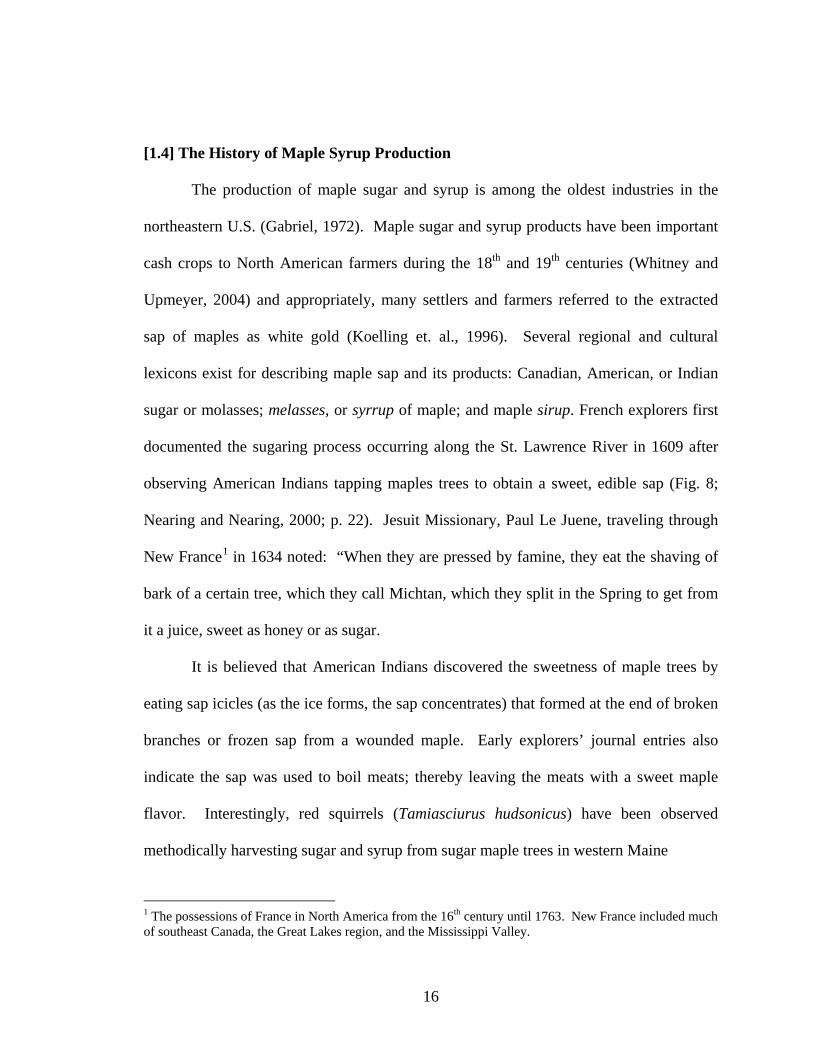
[1.4] The History of Maple Syrup Production

The production of maple sugar and syrup is among the oldest industries in the

northeastern U.S. (Gabriel, 1972). Maple sugar and syrup products have been important

cash crops to North American farmers during the 18th and 19th centuries (Whitney and

Upmeyer, 2004) and appropriately, many settlers and farmers referred to the extracted

sap of maples as white gold (Koelling et. al., 1996). Several regional and cultural

lexicons exist for describing maple sap and its products: Canadian, American, or Indian

sugar or molasses; melasses, or syrrup of maple; and maple sirup. French explorers first

documented the sugaring process occurring along the St. Lawrence River in 1609 after

observing American Indians tapping maples trees to obtain a sweet, edible sap (Fig. 8;

Nearing and Nearing, 2000; p. 22). Jesuit Missionary, Paul Le Juene, traveling through

New France1 in 1634 noted: “When they are pressed by famine, they eat the shaving of

bark of a certain tree, which they call Michtan, which they split in the Spring to get from

it a juice, sweet as honey or as sugar.

It is believed that American Indians discovered the sweetness of maple trees by

eating sap icicles (as the ice forms, the sap concentrates) that formed at the end of broken

branches or frozen sap from a wounded maple. Early explorers’ journal entries also

indicate the sap was used to boil meats; thereby leaving the meats with a sweet maple

flavor. Interestingly, red squirrels (Tamiasciurus hudsonicus) have been observed

methodically harvesting sugar and syrup from sugar maple trees in western Maine

1 The possessions of France in North America from the 16th century until 1763. New France included much of southeast Canada, the Great Lakes region, and the Mississippi Valley.

17

(Heinrich, 1992).

Figure 1.14. A heritage product, maple syrup production is of great pride to a large population of New Yorkers (Photo by author).

18

Figure 1.15. Native Americans collecting sap and cooking maple syrup. Josep Fancois Lafitau, 1724 (Library of Congress).

The storage of liquids posed several problems, and hardened dry maple sugar

could easily be stored. With a stable sugar product, Native Americans of New England

often used the sugar for trading with European explorers presented in the form of a gift.

The popularity of maple products to the early settlers evoked a need to produce these

products for themselves. English settlers were slower to adopt the native’s sugaring

process compared to their French counterparts. The process of sugaring was passed from

Native North Americans to the European explorers and settlers (Heilgmann, et al., 2006).

In the mid- to late-1700s, the production of maple products became an important

19

economic source to many colonists of the Massachusetts Bay Colony, especially where

high transport costs limited the use of imported cane sugar.

The financial capital required to produce sugar was minimal. Therefore, the

advantage maple sugaring offered New England farmers was that it supplied work and

income during the least agriculturally productive season of winter through early spring.

The English scientist William Fox Talbot noted, that maple sugaring can “afford an

ample compensation for the farmer for little more than half a month’s labour.” Families

often made more maple sugar than they could use, and traded the excess for either other

food items or supplies with local merchants. The popularity of the locally-made maple

sugar also highlighted their objection to the sugar cane harvesting by slaves in the West

Indies.

It was not until the 1700s that Europeans developed a need for granular sugar, as

sugar was considered a medicine and luxury item for the wealthy. The blockage of

passage on the St. Lawrence River by the British in 1703–1705, facilitated the need and

production of maple sugar in the Quebec region. During the Napoleonic Wars (1803–

1815), sugar was produced from maple trees in the historical region of Bohemia in

central Europe. The industry received substantial means of encouragement from the

Bohemian government and large groves of maple trees were planted and cultivated.

However, because of the low yields of sugar and the long interval of time required before

trees can be retapped, the industry was short-lived.

20

[1.5] Commercial Aspects of Maple Sugar and Syrup: 1800–Present

Thomas Jefferson was an advocate for the U.S. to produce its own supply of sugar

(i.e., maple sugar), and established a maple plantation at Monticello. The commercial

aspect of the maple sugar and syrup industry did not begin in earnest until the 1800s

(Tyree, 1983), at which time maple products were an inexpensive substitute to offset the

cost of escalating cane sugar prices. With the presence of the American Civil War, many

Northerners saw the consumption of maple sugar as a statement of their abolitionist

beliefs. The rise of the maple sugar industry was short-lived; however, as the increased

availability of sugar derived from sugar cane (Saccharum spp.) post-1803 in Louisiana

and sugar beets (Beta vulgaris) after 1830 created a decrease in the demand for maple

sugar (Whitney and Upmeyer, 2004). Retail prices from Vermont for 1800–1849 show

that maple sugar was consistently less expensive, while during 1850–1859 prices became

approximately equal to that of cane sugar. However, shortages in the supply of cane

sugar during the Civil War (1861–1865) significantly increased prices and cane sugar did

not undersell maple sugar until 1880. With more efficient cane sugar production at the

end of the 19th century, prices fell and the consumption of maple sugar fell while maple

syrup consumption increased (Whitney and Upmeyer, 2004).

New York, Vermont, Michigan, and Ohio were the center of the North American

maple syrup industry from the late-1800s through the mid-1900s. Prior to the 1920s,

80% of worldwide maple syrup production occurred in the U.S. and included several

southern and midwestern states (i.e., North Carolina, Virginia, Kentucky, Tennessee,

Missouri, and Kansas) that have few commercially viable operations. In the 19th century,

21

approximately two-thirds of all Vermont families engaged in maple sugar production and

unlike today, sugar maple was heavily exploited in the Ozark bottomlands of Missouri.

During the later half of the 20th century, the location of peak syrup production

shifted northward with 93% of maple syrup production now occurring in the province of

Quebec, Canada (MacIver et al., 2006). This shift has occurred despite New York alone

having more maple trees than Quebec, and reflects the immense economic support of

their government to underwrite production costs. The Canadian government recognized

early the potential of the industry and made the necessary investments to support its

growth and latter dominance. However, the U.S. has the potential to regain a section of

the international market with investments from federal and state agencies.

Despite this shift, maple production remains an important crop in the northeastern

U.S. Currently (2008), New York produces 20% of the U.S. maple supply, ranking

second to Vermont’s 31%. Further, the economic influence of the industry is significant.

In upstate New York, the total farm cash receipts approach 3 billion dollars on an annual

basis, and maple syrup accounted for greater than 14 million dollars in revenue for 2008

(Keough, 2008). Beyond the economic component of maple syrup, the maple syrup

industry represents a cultural aspect of New England-associated tourism and a way of life

for many long-term residents of the region (Figs. 1.14–1.17).

22

Figure 1.16. American Forest Scene: Maple Sugaring (Currier & Ives, 1856). It was common for artists to use images of "sugaring off" to cleverly comment on the political implications of cane sugar (i.e., slavery). Interestingly, Currier & Ives focused on the community facet of maple sugaring. The firm's 1860 catalogue investigates the social context of maple sugar by describing the image as: "An agreeable picture of a peculiarly American character, showing a maple grove in early springtime. A light snow has apparently fallen over night, and the ground is thinly covered with a mantle of white. On the logs, near the fire where the sap is boiling, are seated two ladies with a male companion, apparently city folks come out to taste the sweets of the country. In the distance, an ox- cart is approaching with another party of the same sort. On the left, two "natives" seem engaged in a discussion, either on the sugar trade or the next election. A number of boys and girls are tending the kettles, bringing up the sap in the buckets, or having a good time generally at the sugaring off." (Springfield Museum, Michele & Donald D'Amour Museum of Fine Arts, Springfield, MA)

23

Figure 1.17 Maple Sugaring: Early Spring in the Northern Woods (Currier & Ives, 1872). [1.6] Harvesting Maple Syrup

Collection

The minimum suggested tree diameter for tapping sugar maples is 10–12 in.

(25.4–30.5 cm) measured at ~breast height (i.e., DBH). Typically, for trees up to 15 in.

(38 cm) in diameter 1 tap is required, 15–20 in. (38–51 cm) 2 taps, and 25+ in. (64 cm)

2–4 taps; some research indicates that using fewer taps-per-tree can substantially increase

the volume of sap-yield-per-tap (Fig. 1.20).

24

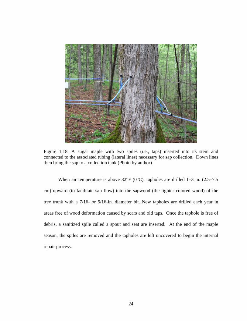
Figure 1.18. A sugar maple with two spiles (i.e., taps) inserted into its stem and connected to the associated tubing (lateral lines) necessary for sap collection. Down lines then bring the sap to a collection tank (Photo by author).

When air temperature is above 32°F (0°C), tapholes are drilled 1–3 in. (2.5–7.5

cm) upward (to facilitate sap flow) into the sapwood (the lighter colored wood) of the

tree trunk with a 7/16- or 5/16-in. diameter bit. New tapholes are drilled each year in

areas free of wood deformation caused by scars and old taps. Once the taphole is free of

debris, a sanitized spile called a spout and seat are inserted. At the end of the maple

season, the spiles are removed and the tapholes are left uncovered to begin the internal

repair process.

25

Figure 1.19 The tree is not harmed from the year-to-year tapping; however, the tree’s response causes staining to the wood which can encompass 3 ft. (~1 meter) vertically up the stem from the taphole (Photo by author).

Traditionally, a metal bucket with a cover, to prevent rainwater and debris

contamination, is hung from the spile with the sap dripping into the bucket. However,

modern collection systems and producers with large operations use plastic tubing and

dark colored pipelines. Sugarhouses and collection tanks are often found at a lower

elevation than the sugarbush and the elevation gradient produces a natural vacuum within

the tubing. However, if a small or no gradient exist, commercial vacuum systems can be

added. Sap is collected daily to help prevent sap from bacterial fermentation and spoiling

and is filtered and stored in large holding tanks (Fig. 1.22). A single tap on average

produces one-quart of syrup; this amount depends strongly on the sugar concentration of

26

the sap. Thus, to produce 200 gallons (53 liters) of syrup, 400–800 tapholes would be

required.

The highest-quality syrup is normally produced soon after the sap is harvested.

Sap from the holding tanks is filtered to remove bark and any other large contaminants.

The sap is then subjected to reverse osmosis to remove large quantities of water before

the costly evaporation process. Next, the concentrated sap enters the wood- or oil-fired

evaporator where the remaining water is evaporated (i.e., boiled off) until the sap (now,

syrup) density is between 66–67% Brix2. This level of density ensures the syrup will

neither ferment nor crystallize.

Annual forecasts of maple syrup production are highly uncertain (Morrow, 1973),

because sap flow (Fig. 1.23) is dependent upon critical changes in temperature during a

relatively short period of alternately freezing and thawing diurnal temperatures. Maple

sap is collected for approximately six to eight weeks each year under specific weather

conditions that occur in northeastern North America from February through April.

Optimal climatic conditions include a combination of nighttime temperature minima

≤32°F (≤0°C), contrasting warm, sunny days 44°F (≥4°C) (Marvin, 1957, 1958), and sub-

freezing soil temperatures that delay budding onset as bud break produces a sour sap and

ends the sugaring season. Producers and researchers have explored the feasibility of fall

(i.e., November) sap collection as similar meteorological conditions could be met and sap

2 Brix is a unit representative of the sugar content of an aqueous solution. One degree Brix corresponds to 1 gram of sucrose in 100 grams of solution.

27

could be obtained. However, for tapped trees, both the amount and the sap-sugar content

of the sap were lower than that obtained in the spring (Koelling, 1968).

Additionally, when springtime yields were compared between trees that were and

were not tapped in the fall, trees tapped in the fall and spring produced significantly less

than trees only tapped in the spring; conversely, no changes in sap-sugar content were

found. These observations provided a strong case for the continuation of springtime

sugaring and the cessation of counterproductive fall tapping.

Figure 1.20. A wounded (i.e., tapped) maple in early spring. Note the darker, wet bark from sap flow (Photo by author).

28

[1.7] Sugarbush Characteristics

Climatic conditions required for prodigious maple sap production limit the

geographical range of the maple syrup industry. Sap used commercially is gathered from

four of the 13 native maple species because of their unique physiology and high sap

yields. In addition to sugar maple, silver maple (A. saccharinum L.), black maple (A.

nigrum Michx. f.), and red maple (A. rubra) are used in the maple industry because of

their high sap-sugar concentration and long sap collection season (Heiligmann and

Winch, 1996).

Interestingly, maple syrup can be produced from the sap of bigleaf maples (A.

macrophytllum) in the Pacific Northwest for noncommercial use. A preliminary study on

bigleaf maple syrup production by Ruth et al., (1972) concluded that commercial

production may be viable; however, syrup produced from bigleaf maples in Corvallis,

Oregon, was of lower quality, with lower sugar content and comparatively less flavor

than the Eastern U.S. standard. Despite the utility of other maple species, no maple

species is as commercially viable as sugar maple. Sugar maples have one of the latest

budbreaks and produce the largest yields of sap with the highest sugar concentrations of

all maple species (Gabriel, 1972).

The maple syrup industry of northeastern North America has historically used

wild sugar maples growing along roadsides, fencerows, or in stands of native forests,

while more recently, sugarbush management has moved toward thinning, phenotypic

stand selection, and cloning of maple saplings selected for high sap concentrations

(Staats, 1994). Maple stands, called sugarbushes, often consist of mature trees.

29

Phenotype variation may also influence sap production as Taylor (1956) observed that

phenotypes within the same sugarbush may have sap-sugar differences of more than

100%, although year-to-year yields of sap-sugar remain consistent (Marvin, 1957).

While many sugarbushes remain in an organic state year-round, as they are free of

chemical treatment(s), commercial fertilizer use can result in a significant increase in sap-

sugar concentrations during the concurrent sap-flow season (Perkins et al., 2004 and

2004). Sugarbush fertilization, however, can decrease the following sugar season’s sap-

sugar concentrations (Watterston et al., 1963), and thus chemical treatments are not

widely used in the northeastern U.S.

Sugar-makers have long recognized the inter-tree variation of the sugar content

and amount of sap produced from their sugarbushes, while often making a point to stop at

a “sweet tree” for a drink. In other words, some trees are significantly more prodigious in

their production of a high sugar content sap. Thus, understanding this variation is

important when trying to reduce the amount of labor required in producing maple syrup

from a dilute maple sap.

Anatomical differences among trees relating to starch storage capacity account for

a minor portion of observed variability in sap-sugar concentrations (Marvin et al., 1967).

The total solids in maple sap vary considerably daily and seasonally for individual trees

and between trees, indicating that optimal conditions for two trees from the same

sugarbush can vary. Thus, it is important to understand the degree of variation between

trees and seasons. Additionally, understanding the influence of environmental factors

30

such as rainfall, light, and temperature that contribute to these variations is important to

maple producers.

Taylor (1945) found that it is difficult to assign a sugar content (percent) value to

a single tree. From the sugar maker’s view, yield of syrup depends on sugar content of

sap and sap flow volume. Early farmers and investigators have been aware of the fact

that maple sap flows occur only following a rise in temperature. However, early efforts

to correlate sap flow rate and volume with temperature were complicated by

understanding which temperature parameter(s) to measure including air, soil, branch,

bark, and trunk (Cortes and Sinclair, 1985). Further, crown health and size, and light

interception are linked to phenotypical differences in sap-sugar concentrations.

In mature stands, maples that produce high-sap-sugar concentrations also produce

the highest sap yields (Marvin et al., 1967). Additionally, the physical characteristics of a

maple tree may provide a diagnostic feature in finding sweet- and high-yield trees.

Specifically: 1) maples with sweeter sap have larger xylem rays than do trees with less

sweet sap (Morselli et al., 1978); 2) maple trees with large crowns such as roadside and

open-field trees tend to produce more and sweeter sap than forest-grown trees (Anderson

1951; Morrow, 1953; Morrow 1955); 3) faster growing mature trees usually are good sap

producers, and sap sweetness increases with tree size (Moore et al., 1951); and, 4) crown

size with trees having a broad healthy canopy is an important positive factor (Anderson,

1951).

Ray parenchyma cells (ray tissue) serve as essential vegetative storage tissues in

which starch, sugars, and protein accumulate seasonally; additionally, is the primary

31

storage areas for sugar in trees (Kramer and Kozlowski, 1979). Attempts to correlate ray

tissue, as a percentage of total-wood volume with sap-sugar concentration to aid in

identifying “sweet” trees has been difficult. Morselli et al., (1978) and Gregory (1981)

report that ray area is strongly correlated with sap-sugar; conversely, Wallner and

Gregory (1980) report that no relationships exist between sap-sugar concentration and the

amount of ray tissue, and that factors other than storage space are involved in regulating

sap-sugar concentrations. Further, both Garret and Dudzik (1989) and Wallner and

Gregory (1980), found a lack of correlation between the amount of sugar storage tissue

(ray cells) and sap-sugar concentrations in sugar maple trees. Annual sap yields are

correlated to the DBH of individual trees, although no relationships were found between

sap sweetness and DBH. Additional studies by Marvin et al., 1967; Blume, 1973; Laing

and Howard, 1990; and Larochelle et al., 1998, support a weak and non-significant

relationship between DBH and sap-sugar concentrations. Crown ratios also are weakly

related to sap and sugar yields in short-term studies (Marvin, 1957).

Conifers in a sugarbush may compete with sugar maples for soil moisture and

nutrients (Walters, 1978). The competition effects can reduce sap flow and lower sap-

sugar concentrations. Studies have shown that a closed sugarbush, with a coniferous

understory composed of hemlock and white pine, consistently produced less syrup

equivalent per-tap than those in an adjacent open, park-like bush. When the understory

was removed, the two sugarbushes produced comparable amounts of syrup equivalent.

Increased availability of nutrients, moisture, and growing space via selective-cutting can

increase tree-growth rates and produce trees with large crowns and higher sap yields

32

(Walters, 1978). The influences of fast growth, increased tree vigor, and large crown

effects on sap and total sugar production were also documented by and Jones et al.,

(1903), Moore et al., (1951) and Blum (1973),

[1.8] Physiology

The success of the sugar maple industry is associated with minor climatological

variations (MacIver et al., 2006) that strongly affect sap production via physiological

responses. Sugar diffusion from the roots into the tree occurs during cold springtime

nights. As air temperatures drop, the branch extremities freeze as does the sap inside of

them, attracting the unfrozen sap from the trunk into the extremities of the branches.

Even though water volume expands upon freezing, maple wood properties provide the

explanation for the unique absorption process.

In sugar maples, unlike in other species, the wood fibers are composed of dead

cells, and those cells contain gas rather than water. These gases contract as temperature

decreases creating space for water to expand upon freezing. In turn, sufficient space

remains for more sap to be drawn by capillary forces from the roots to the branches

through the xylem, creating positive pressure in the stem and thus sap flow (Corte and

Sinclair, 1985).

Positive xylem pressure (sap flow) in sugar maples during early spring has been

recognized and exploited for sugar and syrup production for centuries. The fundamental

phenomenology of this process is well documented (e.g., Jones et al., 1903; Marvin,

1957, 1958; Morrow, 1952, 1955), but the exact mechanism of sap exudation is not

completely understood (Cortes and Sinclair, 1984; Kramer and Kozlowski, 1997; Tyree

33

and Zimmermann, 2003; Cirelli, 2005). In addition to generating hydrostatic xylem sap

pressure, sugar maples also produce a large concentration of sugar in the xylem. The sap

is a dilute solution of water and sugar, along with traces of other non-sugar solids

including organic acids, nitrogenous waste, and inorganic salts. The proportions of sap

are variable and the sugar content, which is 99.9% sucrose, can range from 1–10%, with

2–6% being common. The diurnal behavior of the xylem sap osmotic potential nearly

parallels that of sap hydrostatic pressure, but the connection between these two measures

in sugar maples is indirect (Cortes and Sinclair, 1984). Therefore, the role played by the

concentration of sucrose in the sap in generating hydrostatic pressure may be auxiliary.

[1.9] Meteorological and Climatological Conditions

Because of the known meteorological conditions associated with optimal syrup

production, it is important to understand the relationship between changes in atmospheric

circulation patterns such as the North Atlantic Oscillation (NAO) and seasonal

temperature and precipitation trends. Several studies have found climatological trends

relevant to northeastern U.S. agriculture including: 1) a greater rate of warming

(+1.61°C) during December–February (Keim and Rock, 2001); 2) an average 8-day

increase in growing season length (Easterling, 2002); 3) a decrease in annual and winter

snow-to-total precipitation ratios (Huntington et al., 2004); and 4) an increase in the

frequency of extreme precipitation events (Wake, 2005).

In addition, the NAO, which is a prominent winter teleconnection pattern that,

when positive, produces stronger than average westerlies across the mid-latitudes

bringing mild winters to the Northeast, has been in a positive phase over the past 30

34

years. The magnitude of the positive phase has been unparalleled in the observational

record, with record anomalies occurring since the winter of 1989 (Visbeck et al., 2001).

Because the positive (negative) phase of the NAO can produce winter and early spring

temperatures that are above (below) the long-term mean, this teleconnection may supply

additional warming to an already above-average winter and spring.

Sustainability of a climatically-sensitive industry such as maple sugaring depends

on the ability of farmers to adapt to variable climate conditions. Warmer temperatures,

the frequency and magnitude of insect outbreaks, changes in forest composition, and

invasive plants all threaten the long-term sustainability of the sugar maple industry in

Canada and the U.S. Thus, the decisions of producers to plant seedlings in their aging

sugarbushes may be affected.

The recent decline in maple syrup production parallels the migration of the sugar

maple range and a persistent increase in winter temperatures in this region. Climate

scenarios show a possible shift of two degrees north latitude (from 45°N to 47°N) in the

sugar maple’s current geographical range over the next 100 years with the replacement of

maples with oak, hickory, and pine (Iverson and Prasad, 1998; Beckage et al., 2008; Fig.

1.24).

Even with the use of current technological interventions such as reverse osmosis,

ventless tubing, and vacuum pumping, the production of maple syrup continues to decline

in the northeastern U.S. As ideal meteorological conditions (i.e., number of days with

daily minimum and maximum temperatures 32°F (≤0°C) and 44°F (≥4°C) respectively)

continue to decrease in frequency, the production of maple syrup may become

35

economically unviable for commercial producers. In general, the effects of springtime

warming have been hypothesized by many sugarmakers and extension programs

(MacIver et al., 2006), but no long-term studies have shown empirically how fluctuations

in spring temperatures affect interannual yield.

Figure 1.21. Current mean center and the potential changes in mean center of distribution for sugar maple (Source: Prasad et al., 2007).

The timing of ideal conditions has changed as maple producers throughout New

England report that they are tapping their trees in February and ending the tapping (i.e.,

season) in March. Thus, the sugar season now ends approximately when it began in the

late 19th to mid 20th century (Perkins, 2007). Additionally, producers express concern

36

that the optimal locations for the sugar maple industry will move northward as the

frequency of freeze cycles become increasingly unpredictable. Sugarbushes will also

produce less and lower-quality syrup, while warmer conditions may provide ideal

conditions for the sap to ferment and spoil. Further, above-average winter temperatures

affect the production costs, and during 2003–2007, the price per gallon of syrup increased

58% from $26.80 in 2003 to $42.40 in 2008 (Table 1; Keough, 2009).

37

Table 1. Average maple syrup prices for New York, 1916–2008. Prices are adjusted to 2009 dollars.

Year Price/Gal. Year Price/Gal. Year Price/Gal. 1916 17.52 1947 48.46 1978 39.03 1917 18.24 1948 42.31 1979 38.21 1918 21.19 1949 37.39 1980 39.32 1919 20.09 1950 35.26 1981 41.01 1920 26.54 1951 33.50 1982 37.96 1921 21.99 1952 33.17 1983 36.14 1922 20.30 1953 35.29 1984 34.45 1923 21.19 1954 34.33 1985 33.64 1924 22.39 1955 34.86 1986 37.84 1925 21.84 1956 34.73 1987 43.42 1926 24.03 1957 31.64 1988 42.07 1927 24.50 1958 31.18 1989 40.83 1928 22.59 1959 32.75 1990 38.41 1929 23.33 1960 33.67 1991 36.24 1930 23.29 1961 31.92 1992 35.34 1931 21.07 1962 30.52 1993 27.42 1932 21.78 1963 30.85 1994 35.01 1933 19.67 1964 31.14 1995 32.76 1934 20.61 1965 30.62 1996 34.52 1935 20.88 1966 28.77 1997 33.41 1936 21.44 1967 31.77 1998 35.73 1937 22.18 1968 31.70 1999 34.82 1938 23.36 1969 33.56 2000 35.77 1939 24.45 1970 35.52 2001 35.82 1940 24.21 1971 35.62 2002 37.78 1941 25.22 1972 41.08 2003 31.18 1942 29.29 1973 41.54 2004 29.51 1943 35.58 1974 41.30 2005 34.53 1944 36.20 1975 38.64 2006 33.69 1945 37.15 1976 40.62 2007 34.63 1946 36.41 1977 38.84 2008 42.23

38

With these warming trends, maple syrup production may be inhibited and, in

addition, have a higher sap-to-syrup ratio. Interestingly, when maple producers were

asked to describe the 2005 maple season, which was a low-production year, their major

concerns were: 1) insufficient cold weather; 2) shift toward increased cold in the early

season followed by insufficient late-season cold; and 3) fickle weather that was poor for

sugaring (USDA, 2005). From these observations, it might be hypothesized that maple

syrup production strongly depends upon a balance between the daily minimum and

maximum temperatures. Therefore, diurnal temperature ranges during early spring may

be the central variable in maple yields.

Field studies have examined the short-term effects of daily temperature

fluctuations on pressure formation in dormant maple trunks, which in turn influences sap

yields (Jones et al., 1903; Marvin and Erickson, 1995). Further, the influence of

temperature on sap flow has been examined in controlled experiments (Marvin and

Greene, 1951; Sauter et al., 1973; Tyree, 1983; Cirelli, 2005). These field and laboratory

experiments have shown that sap flow: 1) rates decrease over the long term with several

days without ≤32°F (≤0°C) () temperatures; 2) is weather dependent, and therefore is

often intermittent (i.e., 2–12 sap-runs-per-year); 3) is caused by stem pressure produced

during alternating diurnal cycles of ≤32°F (≤0°C) and ≥32°F (≥0°C); and 4) will not

form in the absence of both freezing and thawing. Further, sap sweetness is highly

influenced by seasonal temperatures and previous year precipitation patterns (Taylor,

1945). In general, the effects of springtime warming have been hypothesized by many

39

sugar-makers and extension programs (MacIver et al., 2006), but no long-term studies

have shown empirically how fluctuations in spring temperatures affect interannual yields.

Several studies have used raw maple syrup production as their variable of interest.

Maple syrup production is not only sensitive to climate but to economic, social, and

political policies (Skinner et al., 2008) as well. Thus, to remove variation in production

caused by non-climatological factors such as the reduction in the workforce of maple

farmers during World War I and II, and to provide a meaningful index of production for

the modeling, I will use the industry standard of yield-per-tap for analyses. Yield-per-tap

is the yearly production of syrup in gallons divided by the number of taps used to collect

the sap and is unaffected by non-climatological trends.

[1.10] Tree-rings

Tree rings of most temperate-latitude species have well-defined increments of

xylem tissue that encircle the entire trunk corresponding to annual growth cycles. The

frequency of species with tree rings is directly related to the seasonality of the climate.

However, not all woody plants produce ring-width sequences that are datable and usable

for climatic inference or ecological studies (Fritts, 1971). In the tropics where

seasonality is limited by the absence of cold winters, many trees do not produce visible

annual rings.

Light intensity and duration, temperature, water, nutrient supply, wind,

mechanical damage to the crown, roots and stem, and pollution of air and soil can affect

tree growth (Schweingruber, 1996). These abiotic factors can influence the rate of radial

growth of the trunk over any temporal period (e.g., months, current year or a previous

40

year (lag)). The information contained in annual tree rings based on width variations is a

valuable resource for studying environmental change. However, identifying the effects

of a single growth factor may be difficult or impossible (Fritts, 1976; Biondi and Waikul,

2004). Often there is irrelevant noise present, and the desired signal must be extracted.

Because of the presence of this noise in the series, a tree-ring series is thought of as a

linear aggregation of several signals that can be interpreted as signal or noise depending

on the hypothesis. Tree-ring growth (Rt) in any one year can be defined by the Principle

of Aggregate Tree Growth (Fritts, 1976)

tttttt EDDCAR ++++= 21 δδ

Where,

A = the age related growth trend due to normal physiological aging processes

C = the climate that occurred during that year

D1 = the occurrence of disturbance factors within the forest stand

D2 = the occurrence of disturbance factors from outside the forest stand

E = random (error) processes not accounted for by these other processes

δ = indicates either a "0" for absence or "1" for presence of the disturbance signal

Dendrochronology is the science of assigning statistically accurate yearly

calendar dates to the xylem growth layers (i.e., tree rings) found in the stems and roots of

woody plants (Fritts, 1971). The strength of this method relies on the ability to

accurately date the year of each growth ring using crossdating. This technique is reliable

41

if the cambial growth in trees responds to environmental conditions that vary yearly. In

certain species, the ring boundaries are difficult to define and occasionally a second ring

(e.g., false ring, double rings, multiple rings, or intra-annual bands) is formed within the

same calendar year. This process is predominantly found in conifers, and their

appearance in dicotyledons is rare, although false rings have been observed in English

oak (Quercus robur) (Schweingruber, 1996). Conversely, trees that grow under intense

competition, on marginal sites, have been severely defoliated or damaged by air

pollution, or are of great age may not produce a growth ring along the entire cambial

surface every growing season. In this case, the ring is considered missing or, more

accurately, locally absent. Rings will often appear somewhere along the circumference

of the tree and therefore, tree slabs (i.e., cookies) are preferred for tree-ring analysis.

Unlike false rings, locally absent rings are common in both conifers and dicotyledonous

trees. The potential for both false and missing rings increases with the age of the tree, the

position of the tree in the canopy (i.e., dominant or subdominant), and the degree of

seasonal stresses.

Many tree species growing in the temperate to Arctic zones produce a distinct

layer of xylem that can be correlated with the growing season. Generally, it is assumed

that each ring represents the product of x year’s growing conditions. However, the

development of a single complete growth ring each year is not a given process (Kramer

and Kozlowski, 1979). Xylem anatomy varies considerably among species and in

different parts of the tree. Angiosperms are classified as ring porous (e.g., oaks, ashes,

and elms) or diffuse porous (e.g., poplars, maples, Figs. 1.25–1.26; and birches). In ring-

42

porous trees, the diameter of the xylem vessels formed early in the growing season are

much larger than those formed later. In diffuse porous rings, all the vessels are relatively

small diameter, and therefore no visible boundary exists between the early and latewood.

Figure 1.23. A macroscopic transverse view of sugar maple wood. Note the numerous, homogenous pores and the slim latewood boundary (Photo by author).

Counting back 100 rings from the cambium along a single radius of the stem does

not ensure that the 100th ring was produced 100 years ago. To aid in crossdating, the list

method is often used whereby years that are narrow are listed for each tree and then are

compared. Typically, within a large sample, a pattern will develop and be used to check

the dating accuracy of the cores. After this, the rings will be measured and the dating is

statistically checked using a computer program called COFECHA (Holmes, 1986; see

methods). If the dating is incorrect and not fixed, the signal strength of past conditions

can be reduced and shifted away from the years in which the actual events such as

droughts or ice storms occurred.

43

In synopsis, dendrochronology is a practical tool when the following conditions

can be met (Telewski and Lynch, 1991):

1) a tree must have a distinct ring boundary;

2) the growth rings must occur on an annual basis;

3) the annual rings must vary either in ring width or in an alterative measurable

feature from ring-to-ring; and

4) the patterns of the ring characteristic must crossdate within the tree and must

crossdate between trees within a study site (and in some cases, between sites).

Typically, when these conditions are met, accurate calendar years are assigned to

each tree ring and statistically verified. Once a series of tree rings (i.e., tree core) are

obtained from several trees at a site and have been crossdated, they are combined to form

a tree-ring chronology that will then be analyzed to obtain climatic or environmental data.

Prior to growth/climate analysis, rings widths are typically standardized through curve

fitting to remove known biological growth trends.

[1.11] Growth and Climate

Temperature is a major limiting factor of tree growth and is apparent in the zonal

growth (i.e., boundary between early and late wood) differences. Within a species, tree

rings are narrower in forests along northern timberlines and larger in warm, moist

regions. However, extreme temperature changes and early- and late-frost can injure the

tree and drastically alter its growth pattern. Both the qualitative and quantitative

properties of temperature influence growth. Absolute values are important, especially

44

based on the season in which they occur and their amplitudes (e.g., maximums and

minimums, cold air out breaks, and heat waves). There are also robust relationships

between tree growth and geographical position including latitude, proximity to the ocean,

distance inland, elevation, and topography (Fritts, 1976). Topographic irregularities, for

example, may influence the duration of snow cover, soil temperatures, and the length of

the growing period. These in effect, alter the complete physiology of the plant, which

are important in the water-conducting and annual growth processes.

The water supply of a region or site has as large of an impact on the trees as

temperature (Kahle, 1994). There are close relationships with geographical location and

moisture availability, e.g., equator (dry), tropics (moist), altitude, and locations along

ocean currents or mountains (wind/leeward). The qualitative and quantitative properties

of precipitation also vary greatly, which—along with the relationship of daily and yearly

cycles—determine plant growth rates. Additionally, the physical properties of the parent

soil are variable, and soils with different compositions dictate the availability of water.

[1.12] Principles

In dendrochronology, the degree to which a tree reacts to environmental factors is

its sensitivity. Sensitivity depends on the tree species and is visible in the tree-ring

sequence. Sensitivity is reflected in the increase in particular narrower or wider tree rings

throughout the series. Mean sensitivity is the measure of change and expresses the

difference between two successive values in a series by means of percentages

(Schweingruber, 1988). It is the average of the absolute values of the individual

45

sensitivities in a series and can be calculated either from raw or standardized values. The

mean sensitivity for a series of rings widths is

where x is either the ring width of the ring-width index for year i, and n is the total

number of rings. The mean sensitivity is a relative measure of the differences and

highlights variation in narrow rings more than variation in wide rings.

By calculating the sensitivity, it is possible to determine the extent to which

growth of an individual species on a particular site is influenced by environmental

factors, both abiotic and biotic. Additionally, periods of growth conditions can be

identified and classified based on whether the ring width variation is stable or variable.

Tree-ring widths that have little variation are referred to as “complacent,” and trees that

have highly variable ring widths are said to be “sensitive.” Complacent tree rings will

have little sensitivity while “sensitive” tree rings will have greater sensitivity. Mean

sensitivity appears to be a strong indicator of the variability of those environmental

factors that fluctuate annually.

Complacent rings indicate uniformity in the affects of climate factors upon the

trees during a succession of years. If rainfall is the limiting factor, the effective rainfall

must be evenly distributed throughout the series of years. Therefore, the trees are assured

a constant supply of moisture and are seldom subjected to periods of drought

(Glock,1939). Further, abundant rainfall evenly distributed over time is stored in the soil,

∑−

= =

+

+−

−

1

1 1

1 )(21

1 n

i ii

ii

xxxx

n

46

acting as a moisture reserve during drier periods. A constant and abundant supply of

moisture tends to form consistently wide rings, while a constant but restricted supply of

moisture tends to cause the formation of consistently thin rings.

Sensitive rings indicate significant departures from uniformity in the climatic

effects upon the trees during a succession of years. Rings typically become more

sensitive in regions close to the forest border and in areas where rainfall averages less

than 10 centimeters per year (Glock, 1939). Differences in ring width in a sequence

appear to vary in proportion to the departures of rainfall from the mean; the greater the

departures, the greater the sensitivity. Sensitive rings indicate an environment in which

annual moisture fluctuates distinctly from year-to-year.

Variations in year-to-year tree-ring widths can serve as natural records of climate

when they represent a limiting factor(s). However, non-climatic factors including fire,

erosional events, changes in water table, lighting strikes, ice- and wind-storms, insect

infestations, nitrogen deposition, and changes in atmospheric CO2 concentrations can

alter tree growth rates (McIver et al., 2007)

Trees are typically selected from sites where ring-widths express significant

interannual variability. Additionally, rings must be crossdated and sufficiently replicated

to provide precise dating and to assure that the inferred climatic “signal” is robust and

properly placed chronologically. Any random error, known as “noise,” from non-

climatic variation in growth, is reduced when ring-width indices are averaged for n many

trees.

47

Dendroecological techniques help evaluate the age structure and tree-growth

patterns to document changing stand conditions either related to disturbance, stand

development, or climatic variation (Payette et al., 1990; Foster et al., 199).

Dendroecological techniques can also help to assess relationships between climate, site

conditions, and tree growth to evaluate factors that influence the growth of a plant

community (Cook and Kairiukstis 1989).

[1.13] Dendrochronology Applications

A basic means of predicting changes in an ecosystem is to create simulation

models of the interactive processes between the ecosystem and its abiotic and biotic

factors. Given the shortage of experimental data from long-term studies, the accuracy of

determining many ecological characteristics is either indefinite or insufficient to make

tangible practical applications (Menshutkin, 1971). To overcome the restraints of

simulation modeling, we will use a dependent set of parameters (i.e., tree-growth)

modeled to a set of environmental factors. These factors will then be used to characterize

a parallel process (i.e., maple syrup production) that is affected by the same

environmental factors.

Dendroecological studies have shown the feasibility of predicting future

behaviors of ecological systems for 5–15 years (Cook and Kairiukstis, 1992). That said,

there are few examples of the use of tree-ring chronologies for yield forecasting with the

exception of the work done by Kairiukstis and Dubinskaite (1986) who investigated the

dynamics of grain crops using a dendrochronological master series from Pinus sylvestris

in Lithuania. The model obtained from their chronology was able to explain 72% of the

48

variance in crop yields, and projections of future yields were validated with the

subsequent harvests. These results suggest the potential for successful forecasting of

other crop yields using tree-ring data.

The application of tree-ring records to estimate previous crop yields was earlier

suggested to discouraged Texas farmers dealing with a string of exceptional dry years by

in 1858 (Campbell, 1949). Because of the lack of meteorological records and

understanding of Texas climate on agriculture at the time, the application of tree rings to

predict agriculture yields allowed farmers to put into perspective the occurrence and

frequency of these exceptional dry years in Texas. More recently, agricultural

reconstructions have been applied to the prehistoric Mississippian societies’ food reserves

in Georgia and South Carolina (Anderson et al., 1995) and for the reconstruction of

historical maize yields for central Mexico (Therrel et al., 2006).

Following the comprehensive work of Fritts (1976), researchers have

implemented standard dendroclimatological techniques to reconstruct a wide variety of

climatic variables extending backward in time beyond the earliest instrumental records.

For example, tree-ring data have been used to reconstruct drought indices, spatio-

temporal patterns of precipitation and temperature, seasonal and annual atmospheric

circulations, stream flow, lake levels, insect outbreaks, ice storms, and volcanic eruptions

(Duvick and Blasing, 1981). Conversely, a limited number of studies have directly

employed tree-ring data to examine crop variability. Tree-ring data obtained from sugar

maples may provide another promising opportunity to determine crop yield, as several

studies have demonstrated the feasibility of the species for dendroecological (e.g., Yin et

49

al., 1994) and dendroclimatological studies (e.g., Lane et al., 1993; Tardif et al., 2001).

Coring practices have been used in the sugaring industry to assess tree growth rates as an

indicator of competition (Heiligmann et al., 2006), but no studies have documented the

application of tree-growth data for syrup yield predictions.

Therefore, understanding the effects that climate variability may have on crop and

pasture yields—including those of maple syrup—has become increasingly important.

Thus, this research will help to promote the effectiveness of using tree-ring data to

predict agricultural yields, which will ultimately provide farmers additional information

about crop yield cycles. This knowledge will in turn help to determine appropriate

management methods for sugarbush operators during less-favorable climatological

conditions. High-quality long-term crop yield data are scarce for many species, and the

use of tree-ring data to reconstruct yield may be a viable method for extending historical

records to examine annual-to-decadal harvest fluctuations.

50

CHAPTER II

METHODS

[2.1] Tree-Ring Data Collection and Field Methods

Data collection, sample preparation, and tree-ring chronology development follow

methodology outlined in Stokes and Smiley (1968) and Fritts (1976). I collected tree-

ring data from six study sites in New York State: 1) Arnot Teaching and Research Forest,

Schuyler County (ASM); 2) Independence River Wild Forest, Herkimer County (IRM);

3) Keeney Swamp State Forest, Allegany County (KSM); 4) Madava Maple Syrup Farm,

Dutchess County, (MDM); 5) R. Milton Hick State Forest, Otsego County (MHM); and

6) the Uihlein Sugar Maple Research & Extension Field Station, Essex County (UUM)

(Figs. 2.1 and 2.2).

[2.2] Regional Forest and Site General Descriptions

2.2.1 The Hemlock–White Pine–Northern Hardwoods Region

This forest region extends from northern Minnesota and extreme southeastern

Manitoba through the upper Great Lakes region and eastward across southern Canada and

New England, toward the southeast, much of the Appalachian Plateau in New York and

northern Pennsylvania. Outliers of the region include the southern Allegheny Mountains

of Pennsylvania, Maryland, and West Virginian. The region has pronounced variations of

deciduous, coniferous, and mixed forest communities.

51

Figure 2.1. Generalized vegetation map of New York (From Braun, 1950).

52

Sugar maple (A. saccharum), beech (Fagus grandifolia), and basswood (Tilia

Americana), sugar maple and beech, or sugar maple and basswood are typically the

dominant primary deciduous communities while yellow birch (Betula alleghaniensis),

white elm (Ulmus americana), and red maple (A. ruba) occur less frequently. Secondary

deciduous communities are composed of aspen (Populus spp.), balsam poplar (P.

balsamifera), paper birch (Betula papyrifera), and gray birch (B. populifolia).

Additionally, two main coniferous communities occur; white pine (Pinus strobus), red or

Norway pine (P. resinosa), and jack pine (P. banksiana) prevail in the sandy plains and

ridges; and in moist, bog or muskeg, areas black spruce (Picea mariana), northern white

cedar (Thuja occidentalis), and larch are dominant. In addition, a third conifer

community of red spruce (P. rubens) occupies mesic flats and slopes in the northeastern

section. The primary mixed communities are hemlock and northern hardwoods or red

spruce and northern hardwoods, hardwood species include sugar maple, beech,

basswood, and yellow birch, with an infusion of white pine.

The boundaries of The Hemlock–White Pine–Northern Hardwoods Region are

poorly defined, and encroaching southern species and migrating northern species

complicate this distinction. The boundaries of this region do not coincide with any soil

province boundaries, but a moderate association between this region and the area of

Podzols exists. The Hemlock–White Pine–Northern Hardwoods Region consists of two

main divisions, the western Great Lakes–St. Lawrence Division and on the eastern side,

the Northern Appalachian Highland Division. The regional division coincides roughly

53

with the topographic break between the physiographic regions and is retained by the

biogeographical range of regional dominate forest species.

2.2.2 Northern Appalachian Highland Division

The Northern Appalachian Highland Division covers the northern Appalachian

Highlands from northern Pennsylvania northeastward across New York, New England,

and the maritime provinces of Canada, and northward onto the plains of Lake Ontario.

The region is marked by mountainous terrain, with more relief than that of the Great

Lakes–St. Lawrence Division. Most of the region experienced glacial activity except for

its southern extension in Pennsylvania. Additionally a great extent of the topography is

controlled by underlying bedrock movement (Braun, 1950).

The North Appalachian Highland Division has three subsections. The Allegheny

section, which includes the entire region south of the Mohawk River and south of the

lowland adjacent to Lake Ontario; the Adirondack section, north of the Mohawk River,

including the Adirondack Mountains; and the New England section, including most of

New England and adjacent areas in Canada (e.g., Acadian Forest region) (Braun, 1950).

2.2.3 Allegheny Section

The Allegheny Section occupies most of northern Pennsylvania and southern New

York. Its southern end in Pennsylvania lies between the northern extensions of the

Mixed Mesophytic region on the southwest and the northern end of the Oak–Chestnut

region on the southeast. Along the area adjacent to Lakes Erie and Ontario, it is in

contact with a section of Beech–Maple region. The Allegheny section includes both the

54

Catskills Mountains and a majority of the Allegheny Mountains of Pennsylvania. This

section occupies the northern end of the unglaciated Alleghany Plateau in northern

Pennsylvania and adjacent New York and all of the glaciated Allegheny Plateau

excluding Ohio and eastern Pennsylvania.

Forest vegetation of the Allegheny Plateau and Allegheny Mountains portion of

the section is similar throughout its boundaries. However, local and regional differences

are often related to soil or moisture profiles. Additionally, forest vegetation of the upland

has been so profoundly modified by lumbering and greater fire suppression activities that

it bears little resemblance to the original cover.

2.2.4 Catskill Mountains

The relief and range of elevation of the Catskill Mountains result in a greater

diversity of vegetation than seen in most regions of the Allegheny Plateau (sans the

Finger Lakes district). Deciduous forest and mixed deciduous-coniferous (e.g., hemlock,

white pine, red spruce, and balsam fir) exist over most of the Catskill Mountains to an

elevation of ~1,068–1,128 meters while Oak of oak–hickory (formerly oak–chestnut)

forest are found in the lowest elevations. In these low-elevation, white-oak dominant

forests, topography often dictates the abundance of red oak, chestnut oak, black oak,

scarlet oak, hickories, historically chestnut, sugar maple, white ash, basswood, butternut,

and white pine.

Above ~368 meters, the hardwood forest dominants are sugar maple, beech,

yellow birch, hemlock, and white pine communities. Sugar maple is prominent and

intermixed with beech, yellow birch, basswood, red oak, butternut, white ash, black

55

cherry, and hemlock. From ~549–610 meters, red spruce and balsam fir become

apparent, marking a transitional forest zone. The transition into Hemlock–White Pine–

Northern Hardwood region is distinguishable by the dominance of maple, beech, yellow

birch, hemlock, white pine, red spruce, and balsam fir.

2.2.5 Adirondack Mountains

The entire area of the Adirondack Mountains experienced glacial modifications.

The eastern part of the Adirondacks is mountainous with two summits above 1,524

meters (5,000 feet) and fourteen other peaks above 1,220 meters. The western part of the

Adirondacks is a dissected plateau of ~610 meters. The elevated regions are

predominantly occupied by deciduous or mixed deciduous–coniferous forests. The

lowlands of the section are occupied by extensions of the oak–chestnut forest and the

hemlock–hardwood forest, both which prevail over the northern Allegheny Plateau.

More characteristic of the Adirondack section are the uplands, which support what may

be termed a mixed or spruce–hemlock–hardwoods, or spruce–hardwoods forest;

however, this varies in composition in relation to soil and moisture regimes and altitude.

The principal species are red spruce, balsam fir, yellow birch, sugar maple, and beech,

with hemlocks and white pines dispersed

56

Figure 2.2. Study sites and the number of maple syrup producers classified based on the modified Jenks’ natural breaks by county.

The six sites were strategically chosen to ensure a comprehensive growth analysis

of sugar maples across the topographically and climatological diverse landscape of New

York (Fig. 2.1 and Table 2.1). New York State is divided into two climatological regions

based on the average position of the convergence of winter Arctic and Pacific Frontal

Zones (Pederson et al., 2004). Accordingly, the sites were appropriately distributed

across the two regions. However, to reduce the variation in tree growth attributed to an

MHM

UUM

IRM

KSM ASM

MDM

57

elevational gradient; all sites are located within 1.4 standard deviations (149 meters) of

the mean site elevation.

Table 2.1 Sugar maple tree-ring chronologies located throughout New York State developed by author.

Sites Elevation (m) Chronology interval

Series length (yrs.)

Mean length (yrs.)

Sample size (cores)

Number of trees

ASM 389 1885–2008 124 108.3 32 23

IRM 460 1796–2009 214 133.7 30 20

KSM 534 1746–2009 264 155.1 32 24

MDM 366 1876–2009 134 93.2 36 28

MHM 606 1784–2008 225 115.6 34 27

UUM 595 1906–2009 104 88.3 33 23

Median 497 - 174 112 32.5 23.5

58

Table 2.2. Generalized site descriptions.

Site Forest Type Predominant Soil Type Slope (%)

1) ASM Allegheny Section

Philo silt loam, Valois gravelly silt loam

3–8

2) IRM

Adirondack Mountains NA NA

3) KSM

Allegheny Section

Ischua channery silt loam 25–35

4) MDM Catskill Mountains Hollis-Chatfield-Rock outcrop complex

>30

5) MHM Catskill Mountains Bath channery silt loam 15–25

6) UUM Adirondack Mountains Adams loamy sand, Croghan fine sand

3–8

During the spring and summer of 2008, 2009 and 2010, I sampled 30 living,

healthy-appearing sugar maples at each site using a 5.15 mm (0.20 in.) Swedish

increment borer. Areas on the tree stem with defects, burls, sigs of dieback, or potential

for rot were avoided (Fig. 2.6). The forests/sampling sites were pre-surveyed for

desirable trees (i.e., potential for individual trees to be at least 110–300 years old) with

the assistance from the New York Department of Conservation’s regional foresters.

Upon arrival to sites, the forests were visually surveyed and tree selections were made

based on generalized old-growth morphological characteristics (Fig. 2.4) (Pederson,

2010) that include large size, gnarled upper limbs; few low living branches (Figs. 2.7 and

2.8). Additionally, attention was paid to topographic position of the trees so that various

aspects, slopes and forest communities were represented.

59

Two cores were extracted at breast height (~1.3 meters) from opposing sides

parallel to slope contours to avoid problems associated with reaction wood (Fig. 2.4).

Therefore, each site contained 60 samples, representing two cores from all trees.

Additionally, while obtaining the core samples, I recorded additional information about

each tree, including basal diameter and crown characteristics.

Figure 2.3. Justin T. Maxwell holding a freshly extracted sugar maple tree core from ASM. Unlike conifers, it is often difficult to visualize the ring boundaries and therefore, estimates of tree age based on visual inspection in the field are hard (Photo by author).

60

Figure 2.4. Coring a shaggy-sugar maple at Independence River Wild Forest, Herkimer County, NY, May 2010. Shaggy bark is thought to be a characteristic of older (>150 years) sugar maples (Photo by Justin T. Maxwell).

I sampled crown codominant and dominant (Fig. 2.5) sugar maples to minimize

forest dynamics effects and thus increase the likelihood that the variability in tree growth

is principally a response to climate variables. The study sites fit several criteria designed

to reduce potential confounding influences associated with anthropogenic disturbance. I

selected areas historically protected by the state government or with known dates of

disturbances such as logging, which allows for a more precise dating of releases or

suppressions. Additionally, I avoided forest parcels with known tree-tapping activity, as

tapping can affect tree growth patterns and vigor (personal observations; B. Chabot,

Cornell University Sugar Maple Extension Program, pers. com., 2010).

61

Figure 2.5. A crown-dominant sugar maple. Note the absence of lower branches. (Photo by author).

62

Figure 2.6. Two sugar maples exhibiting signs (i.e., broken and leafless branches) of dieback. Trees with visuals signs of dieback were not sampled (Photo by author).

63

Figure 2.7. Coring at Keeney Swamp State Forest, Allegany County, NY (KSM). The oldest sugar maple from the six sites, 246 years old (not pictured), was sampled here (Photo by Justin T. Maxwell).

To examine potential changes in growth rates across the time span of human-

caused climate changes (pre- and post-1950), I avoided sampling trees younger than 50

years. Thus, these results indicate the response of mature, wild sugar maple trees that: 1)

germinated before anthropogenically caused changes, and 2) where tree growth,

particularly post-1950, has occurred under rapidly increasing CO2 concentrations that

may have affected growth through atmospheric CO2 fertilization.

64

Figure 2.8. This characteristic understory dominated the six research sites. Photo by Justin T. Maxwell, was taken at the Arnot Teaching and Research Forest, Cornell University, Schuyler County, NY.

65

Table 2.3. Sugar maple tree-ring chronologies series statistics.

Sites Interseries correlation (Pearson's r) Mean Sensitivity Auto Correlation Percent

Missing Rings

ASM 0.691 0.314 0.654 0.606

IRM 0.553 0.294 0.731 0.249

KSM 0.563 0.358 0.776 2.478

MDM 0.611 0.316 0.732 0.388

MHM 0.680 0.376 0.625 0.432

UUM 0.712 0.217 0.635 0.034

Median 0.645 0.315 0.693 0.410 [2.3] Meteorological Data

Mean monthly temperatures and mean monthly precipitation for January–

December were obtained from NY climatic divisions 1, 2, 3, 5, and 10 for the period of

1895–2009 from The National Climatic Data Center (NCDC). State-level mean monthly

temperatures and precipitation, and monthly heating and cooling degree days (HDD and

CDD, respectively) where also obtained from the NCDC for the same period.

[2.4] Maple Syrup Yield Data and Modeling

I used statewide yearly maple-syrup production (gallons) and number of taps

obtained from the United States Department of Agriculture’s National Agricultural

Statistics Service New York Field Station. Typically, production is measured in terms

of the number of gallons produced. “Bumper” years are identified by years of above-

average production preceded by a series of below-average years. Production, as

66

measured by the number of gallons produced in the state does not offer much information

about the efficiency of sap flow for a given year or region. The number of gallons

produced during a season can be influenced by the physical environment (e.g.,

meteorological) as well as other variables including the number of producers and trees

tapped and season start and end dates. To adjust for these factors and to provide a

measure expressing the meteorological-based variation in yield, the industry standard,

Yield-per-Tap, is commonly used. Thus, this measure allows practical comparisons

between years and regions where syrup is produced.

Previous studies have used raw maple syrup production (i.e., gallons produced) as

their variable of interest (cf Whitney and Upmeyer, 2004). However, maple syrup

production is not only sensitive to climate, but to economic, social and political policies

(Chabot et al., 2008). Thus, to remove variation in production caused by non-

climatological factors including a decline of maple farmers during WWI and WWII, and

to provide a meaningful index of production for my modeling, I used the industry

standard of yield-per-tap for analysis. Yield-per-tap is the yearly production of syrup in

gallons divided by the number of taps used to collect the sap and is independent of non-

climatological trends.

I used multivariate regression analysis to produce the best model and to determine

which variables account for the variation in maple syrup yield. Because of the

complexity of ecophysiological processes, the initial number of predictors (20–30) was

relative to the complexity of the system being studied (Kairiukstis and Dubinakaite,

1986). To reduce estimation bias, I used Mallow’s Cp Statistic, Predicted-R2, and the

67

Variance Inflation Factor (VIF) as regression diagnostics. The meteorological predictors

were then modeled with the variable yield-per-tap obtained through the United States

Department of Agriculture National Agricultural Statistics Service New York Field

Office.

[2.5] Lab Methods

Increment cores were allowed to air dry and then mounted onto a wooden core

mount with the cells aligned vertically so that the ring boundaries were visually apparent

after sanding. The cores were sanded using progressively finer sandpaper, beginning with

ANSI 120-grit (105–125 μm) and ending with ANSI 600-grit (26–29 μm). The sanding

process allowed the cellular structure of the tree rings to be visible under standard 10X

magnification.

I crossdated my samples using visual and statistical crossdating techniques to

assign calendar years to each ring in my samples. I also used the list method by

identifying and recording notable marker rings to assist in crossdating (Yamaguchi,

1991). Visual crossdating was accomplished through recognition of patterns of wide and

narrow rings common to all my sites (Fritts, 2001). This procedure also accounted for

locally absent and false rings.

Each set of raw tree-ring measurements was evaluated using the computer

program COFECHA (Holmes, 1983) to ensure proper crossdating and assess series

correlation and mean sensitivity of ring widths (Table 2.3). The COFECHA program

analyzed patterns in the ring- width measurement series of each individual sample from a

data site and detected (flags) possible errors in crossdating. The assignment of flags by

68

COFECHA to individual samples in a data set can guide a reconsideration of the

crossdating of increment core samples. Cores that correlated poorly in COFECHA were

removed from the population prior to chronological development in ARSTAN. Cores

that were removed had Pearson’s r-values of <0.450, or in some cases, the core was

stripped in length to remove low correlating 50-year segments if sample depth was

needed. However, COFECHA allowed only a statistical analysis of the similarity

between the individual time series at the site. Further examination of the physical samples

may indicate that COFECHA, rather than the crossdating procedure, was in error (Fritts,

1991). COFECHA provides two other critical measures of the quality of a tree-ring data

set. First, the program assesses the inter-series correlation of each sample at a site; a

mean inter-series correlation above 0.40 is considered desirable (Holmes, 1983). Second,

the program provides the mean interannual sensitivity of all samples. Higher mean

sensitivity at a site may indicate a greater likelihood of a strong growth-limiting signal,

often climate-related (Stahle and Cleaveland, 1992).

After crossdating the cores, individual ring widths were measured to an accuracy

of 0.001 mm using a linear encoder. I used the program ARSTAN (Cook and Holmes,

1985) to develop the standardized chronology for each site. In order to preserve low-

frequency signals that may contain oceanic atmospheric teleconnections, I employed

conservative standardization techniques such as fitting a negative-exponential curve or a

negative linear curve for the development of our chronologies (Figs. 2.9 and 2.10).

Additionally, if stand dynamics were present (i.e., growth effects of canopy openings,

windfalls, ice storms) a Freidman super smoother (Fig. 2.11) was used to reduce the

69

influence of short periods (3–5 years) of suppressed or abrupt growth at that may be

caused by stand dynamics present in the tree-ring time series while simultaneously

preserving long-term trends.

Figure 2.9. Raw ring-width measurements exhibiting a negative linear growth pattern (top). The raw series is detrending using the fitted linear model and is then standardized (bottom).

70

Figure 2.10. Raw ring-width measurements exhibiting negative exponential growth (top). The raw series is detrending using the fitted exponential model and is then standardized (bottom).

Figure 2.11. Due to forest dynamics, in some cases neither a negative linear nor negative exponential model can be used for detrending. Therefore, a Friedman super smoother curve is fitted to reduce the effects of short periods (ca. 1860) of growth releases.

71

After detrending, each series of tree growth are averaged using a biweight robust

mean function to create the mean value function for each population of trees (Pederson et

al., 2004). Using a biweight robust mean will reduce the effects of outliers for individual

tree-ring series in the chronology (Cook and Holmes, 1992). To capture the climate

signal, a residual chronology, which contains the least amount of disturbance-related

growth and lacks autocorrelation (Cook, 1985), was evaluated for possible selection for

use in the development of growth-climate models.

Chronology reliability (i.e., quality) was estimated using the metrics rbrar (Briffa,

1995) and expressed population signal statistics (EPS) (Wigley et al., 1984). EPS and

rbar are the chief diagnostics tools in testing chronology reliability for climatological

studies and, to a lesser degree, in ecological studies. Rbar is independent of sample size

and unbiased, and is the mean correlation of all growth series (i.e., cores) within a

population of sampled trees (Fig. 2.12). EPS is a function of rbar and sample size and

describes how well a finite sample size estimates an infinite, hypothetical population

(Fig. 2.12). Chronology lengths were then stripped to the year that corresponded with an

EPS value ≥0.85 (Fig. 2.12; Cook et al., 1992)

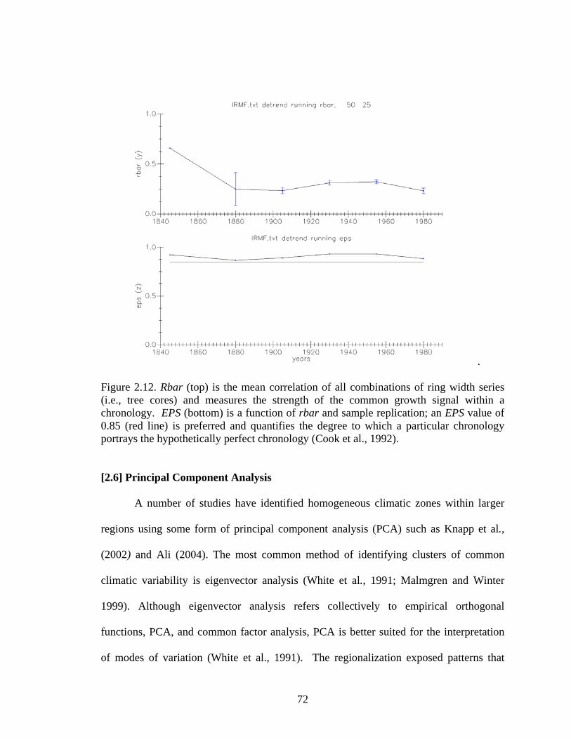
72

.

Figure 2.12. Rbar (top) is the mean correlation of all combinations of ring width series (i.e., tree cores) and measures the strength of the common growth signal within a chronology. EPS (bottom) is a function of rbar and sample replication; an EPS value of 0.85 (red line) is preferred and quantifies the degree to which a particular chronology portrays the hypothetically perfect chronology (Cook et al., 1992). [2.6] Principal Component Analysis

A number of studies have identified homogeneous climatic zones within larger

regions using some form of principal component analysis (PCA) such as Knapp et al.,

(2002) and Ali (2004). The most common method of identifying clusters of common

climatic variability is eigenvector analysis (White et al., 1991; Malmgren and Winter

1999). Although eigenvector analysis refers collectively to empirical orthogonal

functions, PCA, and common factor analysis, PCA is better suited for the interpretation

of modes of variation (White et al., 1991). The regionalization exposed patterns that

73

allowed correlation analyses with atmospheric teleconnection features and regional

climatic data.

Climatic regionalization is inherent to tree-ring reconstructions of climate. Tree-

ring data from a given location often have strong correlations with climate data in a larger

surrounding region (Griggs et al., 2007; Akkemik et al., 2008). Tree-ring data may have

also correlated strongly with climate data in areas far removed (e.g., > 200 km) from the

data-collection sites (Stahle and Cleaveland, 1992; Griggs et al., 2007). Regions with

strong correlations between instrumental climate data and tree-ring data are considered

homogeneous climatic regions, despite observed variability within the identified region

(Stahle and Cleaveland, 1992; Griggs et al., 2007).

I compiled and analyzed radial-growth indices from each site using Eigenvector

analysis. My study employed S-mode PCA, the most commonly cited approach for

climatic analysis (Kolivras and Comrie 2007; Timilsena and Piechota, 2007).

The fundamental goal of PCA is to express a majority of the variance in the

original data in a smaller number of variable dimensions, thereby reducing complex data

sets to physically interpretable abstractions (White et al., 1991; Malmgren and Winter,

1999). In practice, a small number of PCs can often account for as much variance as the

original variables by discounting noise in the data. Regardless of the procedure, the PCs

are orthogonal (uncorrelated), with the first PC accounting for as much of the variance as

possible. Each successive PC accounts for the maximum possible remaining variance.

Principal components explaining a substantial portion of the total variance can be

extracted with various applications based on the objectives of the analysis (Cattell 1966).

74

After an initial S-mode PCA retaining all factors, the investigator selects one to

several PCs for further analysis. Retention of too few components may oversimplify

spatial patterns, while the retention of too many involves the inclusion of increased noise

in the data. In turn, over-retention may distort spatial patterns and lead to splintering of

spatial units (Richman, 1986). A common approach for PCs retention is based on scree-

plot evaluation (Cattell, 1966). The plot shows the curve of explained variance associated

with each successive PC. A leveling-off of the scree plot indicates a substantial reduction

in explained variance by the addition of more PCs, and provides a valuable guide for

selecting a range of factors to retain. However, no method insures extraction of the

correct number of PCs. The results must come from PCs that display logically

interpretable patterns (Cattell, 1966).

[2.7] Growth-Climate Analysis

Step one of climate analysis was to determine climate variables significantly

related to sugar maple growth at the six sites. I used two techniques, correlation analysis

and response-function analysis, to test the growth response to climate. I used

DENDROCLIM2002, a dendroclimatic analysis program (Biondi 1997; Biondi and

Waikul 2004), for both analysis types. PRECON (Fritts, 1991) is an alternative software

program that develops a bioclimatic model of tree growth and calculates the explained

variance of each climate variable using response function analysis (RFA). However,

DENDROCLIM2002 is preferred first because of its user friendly interface and secondly

because the bootstrapped confidence intervals are calculated for both correlation and

response functions. Bootstrapping was added to this technique in order to avoid bias,

75

limit error, and achieve more accurate results (Guiot, 1991; Biondi and Waikul, 2004).

DENDROCLIM 2002 checks the statistical significance of response function coefficients

with the bootstrap method and highlights coefficients exceeding the 95% significance

level (Biondi, 1997; Biondi and Waikul, 2004). This ensures accurate testing for

significance of variables (Biondi and Waikul, 2004) and even in the presence of

autocorrelated data. DENDROCLIM2002 assumes data to be normal and therefore the

correlation analyses generates Pearson product-moment correlation coefficients (r)

between monthly climate variables and ring-with indices.

[2.8] Correlation Analysis

Within DENDROCLIM2002, the Pearson product-moment correlation coefficient

is calculated between each year’s ring-width index and monthly climate variables from

June of the previous growing season to November of the current growing season. I

calculated correlation coefficients from 1910 to the most recent common growth year,

2007.

[2.9] Response Function Analysis

Originally developed by Fritts (1991), response function analysis (RFA) uses

principal components multiple regression to eliminate the effects of interdependence

among climate variables (Fritts et al., 1971; Fritts, 1976). Like correlation functions, RFA

indentifies monthly climate variables significantly affecting tree growth.

DENDROCLIM2002 uses bootstrapped confidence intervals to comprehensively test for

significance (Biondi and Waikul, 2004).

76

I conducted response function analyses to complement the correlation analyses of

the climate-tree growth relationship. RFA is a widely applied technique that uses

principal components multiple regression to estimate indexed values of ring-width

growth. The products of the regression coefficients and the principal components are

calculated to obtain a new set of regression coefficients related to the original climate

data (Briffa and Cook, 1990; Biondi and Waikul, 2004). An advantage of RFA over

correlation analysis is that RFA removes the effects of interdependence among the

climate variables (Fritts, 1976). When correlation and RFA are conducted together in

DENDROCLIM2002, RFA typically identifies fewer significant relationships than

correlation analysis.

[2.10] Moving Correlation Analysis

After the initial correlation and RFA, I performed moving-correlation analysis

between growth and monthly precipitation, temperature, and PDSI at moving x-year

intervals using DENDROCLIM2002. Biondi and Waikul (2004) suggest a window length

of at least twice the number of predictor months. For precipitation and temperature the

period of analysis was the common period of all chronology, 1910–2007.

The objective of this analysis was to test for temporal changes in the climate-tree

growth relationship (Biondi, 1998; Biondi and Waikul, 2004), including complete shifts

to which variables a tree, or stand of trees, responds and changes in response strength. A

consistent response to a given climate variable indicates that a dataset may have climate

reconstruction potential. The results of moving correlation analysis will be displayed

individually for each variable (monthly mean temperature and precipitation) using the

77

standard graphical outputs from DENDROCLIM2002. Intervals during which a variable

was not significantly correlated to tree growth are shaded green, while significant

correlations are colored according to the strength of the correlation coefficient

Analyzing the changing relationships between tree growth and climate has a long

history within dendroclimatology (Visser and Molenaar, 1987), with increasing

importance since the identification of the divergence problem (Briffa et al., 1998; Esper

and Frank, 2009). In the 1980s, Van Deusen (1987) and Visser and Molenaar (1987)

applied the Kalman filter to dendrochronology. The Kalman filter has been used to create

tree-ring chronologies from numerous ring-width series and to generate predictors of tree

growth, based on climate variables that can change temporally (Van Deusen, 1987). This

technique indicates if correlations levels of specific climate predictors are stable and has

been used to analyze tree growth-climate relationships in the eastern U.S. The earlier

work of Van Deusen (1987) and Visser and Molenaar (1987) suggested that the climate

variables that affect tree growth today might not be the same variables that affected past

tree growth. Significant climate response variations throughout the calibration period

compromises reconstruction reliability.

[2.11] Reconstruction

I used a two-stage process of calibration and verification to develop the yield-per-

tap (i.e., syrup yield) reconstruction. Simple correlation analysis between the tree-ring

chronologies and yield-per-tap was used to determine the reconstruction potential. I then

used calibration and verification tests of the reconstruction model for two periods: 1916–

1960 and 1961–2006 and developed a yield-per-tap regression model for 1960–2006

78

using tree-ring chronology indices as the dependent variable and the yield-per-tap as the

independent variable.

The resulting predicted values obtained from linear regression models were

verified against the observed yield-per-tap for the independent period (1916–1960). I

repeated this procedure using the earlier period (1916–1960) as the dependent period and

latter half (1961–2006) as the independent period used for verification. I checked the two

calibration models for statistical significance using several verification tests. The

verification procedures assessed whether the model accurately replicated the observed

data (i.e., the independent period not used to calibrate the model). The reliability of the

reconstruction was assessed using the Pearson correlation coefficient; the reduction of

error statistic (RE) (Fritz, 1976)

( )

−−=∑ 21

ci

v

YYSSRRE

where SSR equals the sum of squares residuals from the verification period and iY and

cY are the actual period and calibration mean period predictands, respectively; and the

coefficient of efficiency (CE), an extremely stringent statistic used to estimate the

verification period R2 (Nash and Sutcliffe, 1971)

( )

−−=∑ 21

vi

v

YYSSRCE

79

where vY is the mean of the actual data in the verification period. Therefore, if vY = cY ,

then CE = RE, if however, vY ≠ cY , then CE < RE. RE and CE have a theoretical range of

−∞ to 1.0, and CE and RE values >0 are usually interpreted as an indication of regression

model validity (Cook, 1997). Additionally, since the verification and calibration period

means will almost never be identical, CE will almost always be less than RE, therefore, a

positive CE is more difficult to obtain.

80

CHAPTER III

RESULTS [3.1] Principal Components

Two procedures were used to ensure statistical validity of tree-ring data reduction

when using principal components analysis. The Kaiser-Meyer-Olkin Measure (KMO) of

Sampling Adequacy test-statistic varies between 0 and 1, and values closer to 1 indicate

that patterns of correlation are sufficiently compact and factor analysis should yield

distinct and reliable factors. A value of 0.500 is suggested by Kaiser (1974) as the

minimum. Bartlett's Test of Sphericity tests the null hypothesis that the correlation

matrix is an identity matrix, which would indicate that the factor model is inappropriate.

Thus, rejecting the null hypothesis is most favorable. Together, these tests provide a

minimum standard, which should be passed before a principal components analysis,

should be conducted. Using the aforementioned criteria, the tree-ring data passed the

initial diagnostics: KMO measure = 0.622, and therefore, > 0.500; and Bartlett’s Test of

Sphercity p < 0.05 (Table 3.1).

Table 3.1. Results of KMO Measure and Barlett’s Test of Sphericity.

Kaiser-Meyer-Olkin Measure of Sampling Adequacy 0.622

Bartlett's Test of Sphericity Approx. Chi-Square 176.540

Degrees of freedom 21 p-value 0.000

81

Significant correlations among site chronologies using Pearson’s r varied between

0.238 and 0.683 (Table 3.2) with inter-site proximity positively affecting correlations.

IRM and MHM have the highest median correlations with all sites (0.294 and 0.300;

respectively). The input matrix for the first-run, unrotated S-mode PCA consisted of

seven variables representing the individual tree-ring chronologies and 97 observations

representing annual growth index values for the common period 1910–2007. The results

of the first-run, unrotated S-mode PCA retaining all factors (n = 7) determined that the

first three PCs of tree-ring data explained 69.96% of variance (Table 3.3) among the tree-

ring chronologies and eigenvalues for only PCs 1–3 were >1 (Fig. 3.1). Additionally, the

scree plot indicated a leveling off (Fig. 3.1) in explained variance after the third PC.

Therefore, I proceeded by retaining only the first three PCs in order to determine the

number of subregions that were logically and physically interpretable. The data were then

submitted to PCA with and a varimax rotation using the three retained PCs.

In general, the results of unrotated PCA do not yield physically interpretable

patterns of climate behavior (Richman, 1986). The varimax rotation technique is the

dominant orthogonal rotation identified in the climate literature (Malmgren and Winter,

1999; Timilsena and Piechota, 2007). After rotation, the subregions showed no signs of

splintering and were spatially contiguous (i.e., stabilized) when three PCs were retained.

The chronologies were grouped according to the loading scores on the three PCs, which

reflected spatial patterns of variance in the selected tree-ring data across New York.

82

Figure 3.1. Scree plot for unrotated S-mode PCA. Table 3.2. Correlation matrix for all tree-ring sites (significant values are bold).

Site MHM MDM KSM IRM UUM ASM r-value MHM 1.000 −0.006 0.298 0.341 0.290 0.242

MDM −0.006 1.000 −0.091 −0.015 −0.054 0.006 KSM 0.298 −0.091 1.000 0.323 0.228 0.683 IRM 0.341 −0.015 0.323 1.000 0.405 0.282 UUM 0.290 −0.054 0.228 0.405 1.000 0.311 ASM 0.242 0.006 0.683 0.282 0.311 1.000

p-value MHM - 0.477 0.001 0.000 0.002 0.008

MDM 0.477 - 0.186 0.440 0.297 0.476 KSM 0.001 0.186 - 0.001 0.011 0.000 IRM 0.000 0.440 0.001 - 0.000 0.002 UUM 0.002 0.297 0.011 0.000 - 0.001 ASM 0.008 0.476 0.000 0.002 0.001 -

83

Table 3.3. Total explained variance for the three components before and after varimax rotation.

Component Extraction Sums of Squared Loadings

Rotation Sums of Squared Loadings

Total % of Variance

Cumulative % Total % of

Variance Cumulative

% 1 2.675 38.210 38.210 1.953 27.897 27.897 2 1.219 17.414 55.624 1.934 27.627 55.525 3 1.003 14.332 69.955 1.010 14.431 69.955

Table 3.4. Rotated component matrix.

Component 1 (Eastern) 2 (Western) 3 (Hudson Valley) MHM 0.867 0.151 0.025 UUM 0.453 0.402 −0.101 KSM 0.088 0.879 −0.069 ASM 0.117 0.875 0.058 IRM 0.446 0.458 −0.014 MDM −0.011 −0.022 0.995

Principle components revealed three distinct geographical subregions that were

divided longitudinally: Region 1 including sites MHM and UUM located in eastern NY;

Region 2 including sites ASM-KSM-IRM are located in western NY; and Region 3

comprised of site MDM, located in the Hudson Valley. Interestingly, MDM falls into its

own component (3), possibly because it is the south-easternmost site and located in the

Hudson River Valley; an area know to be a plant-climate transition zone. These results

differ from what would be expected given the recognized statewide latitudinal-

climatological boundaries.

84

[3.2] Modeling Maple Syrup Yield and Meteorological Data 3.2.1. Step-Wise Regression, Yield-Climate Model I

Independent variables used were January–December of previous-year mean

monthly temperature, mean monthly precipitation, January–April of the current-year

mean monthly temperature, and mean monthly precipitation. The total number of initial

variables n = 32. Alpha-to-Enter of 0.10 and Alpha-to-Remove of 0.15 were used to

select initial variables. The response variable is NY syrup yield for 1916–2008, n = 91.

After the addition of the 6th variable, Mallow’s Cp fell below the optimal value (Table

3.5). The most adequate model will have the lowest Mallow’s Cp value that is

approximately equal to the number of predictors plus one (i.e., p). Despite improvements

to the R2 (30.18% v. 32.55%), R2-adjusted (25.31% v. 26.99%), and R2-predicted (17.65%

v. 19.03%), Mallow’s Cp becomes < p (i.e., 6.9), which indicates an over fitting of the

model. The selected variables are consistent with known meteorological parameters that

affect syrup yield.

85

Table 3.5. Order of insertion of possible yield predictors used for step-wise regression fitting for yield-climate model I. Yellow shading indicates selected model.

Step 1 2 3 4 5 6 Constant 0.287 0.337 0.344 0.167 0.143 0.220 Mar Temp −0.003 −0.003 −0.003 −0.003 −0.003 −0.002 T-value −3.310 −3.770 −3.130 −3.110 −3.370 −2.660 p-value 0.001 0.000 0.002 0.003 0.001 0.009 Jan Temp −0.002 −0.002 −0.002 −0.002 −0.002 T-value −2.810 −2.980 −3.130 −3.390 −3.500 p-value 0.006 0.004 0.002 0.001 0.001 Junp Prec −0.006 −0.005 −0.005 −0.004 T-value −2.160 −1.910 −1.730 −1.560 p-value 0.034 0.060 0.087 0.122 Junp Temp 0.003 0.003 0.003 T-value 1.740 1.790 1.820 p-value 0.086 0.076 0.072 Feb Temp 0.001 0.002 T-value 1.740 2.130 p-value 0.086 0.036 Apr Temp −0.002 T-value −1.930 p-value 0.056 R2 10.74 17.94 22.02 24.61 27.14 30.18 R2-adjusted 9.76 16.12 19.39 21.18 22.96 25.31 Mallow’s Cp 22 15 12 10.7 9.6 7.8 R2- predicted 6.24 11.98 14.98 15.37 16.2 17.65

86

Table 3.5. Continued. Step 7 8 9 Constant 0.344 0.332 0.336 Mar Temp −0.003 −0.003 −0.003 T-value −2.930 −3.350 −3.250 p-value 0.004 0.001 0.002 Jan Temp −0.002 −0.002 −0.002 T-value −3.440 −3.380 −3.420 p-value 0.001 0.001 0.001 Junp Prec −0.004 T-value −1.430 p-value 0.158 Junp Temp 0.003 0.004 0.004 T-value 2.060 2.290 2.380 p-value 0.043 0.024 0.019 Feb Temp 0.002 0.002 0.002 T-value 2.190 2.370 2.580 p-value 0.031 0.020 0.011 Apr Temp −0.002 −0.002 −0.002 T-value −1.850 −1.970 −2.010 p-value 0.068 0.052 0.048 Sepp Temp −0.003 −0.003 −0.003 T-value −1.730 −1.850 −1.890 p-value 0.088 0.068 0.063 Mayp Prec −0.005 T-value −1.780 p-value 0.079 R2 32.55 30.94 33.41 R2-adjusted 26.99 26.12 27.93 Mallow’s Cp 6.9 6.9 5.8 R2- predicted 19.03 18.68 19.69

87

3.2.2 Final Model for Step-Wise Regression yield-climate model I

The final yield-climate model I is:

( ) ( ) ( )

( ) ( ) ( )AprtempFebtemptempJunprecpJunMartempJantempYield

p

p

⋅−⋅+⋅+

⋅−⋅−⋅−=

00254.000186.000281.0

00352.000213.000253.0215.0

and has an R2 = 33.70%, p < 0.001; a D-W statistic = 1.94 (95% CI, 1.38;1.66); and

normally distributed residuals (Figs. 3.6 and 3.7; Table 3.6). This model indicates that

NY maple syrup yield responds to mean January, March, and April temperatures

inversely, where warmer mean temperatures reduce syrup production and cooler spring

temperatures increase sap yields. Conversely, the positive mean February coefficient

indicates increased syrup production for warmer Februarys. Additionally, previous June

(i.e., 2010 syrup season = 2009 summer conditions) precipitation and temperature have a

negative and positive affect of syrup yield, respectively. Mean March and previous mean

June precipitation and previous mean June temperature are the strongest predictor

variables, accounting for 22.00% of the 33.70% explained variance.

Table 3.6. Model Statistics and Diagnostics for yield-climate model I.

R2 33.70% R2-adjusted 28.90% Durbin-Watson statistic 1.94 R2-predicted 22.01% Cp statistic 7.80

88

Table 3.7. Variable coeffients and diagnostic values for yield-climate model I.

Predictor Coefficient SE Coefficient T-statistic p-value VIF Constant 0.2152 0.1070 2.01 0.048 Jan Temp −0.0025 0.0006 −4.14 0.000 1.04 Mar Temp −0.0021 0.0009 −2.43 0.017 1.20 Junp Prec −0.0035 0.0024 −1.45 0.151 1.14 Junp Temp 0.0028 0.0014 1.96 0.053 1.04 Feb Temp 0.0019 0.0007 2.60 0.011 1.11 Apr Temp −0.0025 0.0012 −2.20 0.030 1.18 Table 3.8. ANOVA table. for yield-climate model I. Source DF SS MS F-statistic p-value Regression 6 0.0350 0.0058 7.11 0.000 Residual Error 84 0.0689 0.0008 Total 90 0.1038

420-2-4

99.9

99

90

50

10

1

0.1

Standardized Residual

Per

cent

0.240.210.180.150.12

2

1

0

-1

-2

Fitted Value

Stan

dard

ized

Res

idua

l

210-1-2

20

15

10

5

0

Standardized Residual

Freq

uenc

y

9080706050403020101

2

1

0

-1

-2

Observation Order

Stan

dard

ized

Res

idua

l

Normal Probability Plot Versus Fits

Histogram Versus Order

Figure 3.2. Residual plots for yield-climate model I.

89

0.100.050.00-0.05-0.10

99.9

99

9590

80706050403020

10

5

1

0.1

Residuals

Perc

ent

Mean -2.10149E-16StDev 0.02766N 91AD 0.305P-Value 0.562

Probability Plot of ResidualsNormal

Figure 3.3. Normality plot of residuals for yield-climate model I. 3.23 Step-Wise Regression, Yield-Climate Model II

Independent variables used were identical to yield-climate model I step-wise

regression with the addition of January–December of previous year Heating Degree Days

(HDD) and Cooling Degree Days (CDD); and January–April of current year HDD and

CDD. Again, an Alpha-to-Enter of 0.10 and Alpha-to-Remove of 0.15 was used.

Response variable is NY syrup yield on 64 predictors, n = 91. After the addition of the

7th variable, Mallow’s Cp fellow below the optimal value. Despite improvements to the

R2 (41.11% v. 47.64%), R2-adjusted (39.40% v. 42.54%), and R2-predicted (33.33% v.

35.66%), Mallow’s Cp becomes < p (Table 3.9), which indicates model over fitting.

90

Table 3.9. Order of insertion of possible yield predictors used for step-wise regression fitting for yield-climate model II.

Step 1 2 3 4 5 6 Constant 0.205 0.251 0.313 0.071 0.060 0.000 Mar CDD −0.001 −0.001 −0.002 −0.002 −0.001 −0.001 T-Value −3.070 −3.500 −4.190 −4.360 −4.140 −4.340 p-Value 0.003 0.001 0.000 0.000 0.000 0.000 Jan Temp −0.002 −0.002 −0.003 −0.003 −0.003 T-Value −3.280 −3.820 −4.200 −4.650 −4.760 p-Value 0.001 0.000 0.000 0.000 0.000 Feb HDD 0.000 0.000 0.000 0.000 T-Value −2.780 −2.930 −2.770 −2.460 p-Value 0.007 0.004 0.007 0.016 Junp Temp 0.004 0.004 0.004 T-Value 2.710 2.920 2.960 p-Value 0.008 0.004 0.004 Julp HDD −0.032 −0.032 T-Value −2.450 −2.560 p-Value 0.016 0.012 Augp CDD 0.000 T-Value 2.550 p-Value 0.013 R2 9.60 19.46 26.02 31.86 36.30 40.93 R2-adjusted 8.58 17.63 23.47 28.69 32.62 36.71 Mallow’s Cp 47.0 34.3 26.6 20.0 15.3 10.5 R2- predicted 4.77 13.85 19.29 23.15 28.04 31.47

91

Table 3.9. Continued. Yellow shading indicates selected model.

Step 7 8 9 Constant 0.146 0.149 0.158 Mar CDD −0.002 −0.002 −0.002 T-Value −4.700 −5.030 −4.890 p-Value 0.000 0.000 0.000 Jan T −0.003 −0.003 −0.003 T-Value −4.710 −4.690 −5.000 p-Value 0.000 0.000 0.000 Feb HDD 0.000 0.000 0.000 T-Value −2.720 −3.190 −3.190 p-Value 0.008 0.002 0.002 Junp Temp 0.004 0.005 0.005 T-Value 3.260 3.750 3.660 p-Value 0.002 0.000 0.000 Julp HDD −0.030 −0.025 −0.025 T-Value −2.450 −2.030 −2.090 p-Value 0.016 0.045 0.040 Augp CDD 0.000 0.000 0.000 T-Value 2.530 3.020 3.170 p-Value 0.013 0.003 0.002 Sepp Temp −0.003 −0.003 −0.003 T-Value −2.170 −2.460 −2.520 p-Value 0.032 0.016 0.014 Janp Temp −0.001 −0.001 T-Value −2.350 −2.330 p-Value 0.021 0.022 Dec CDD 0.002 T-Value 1.760 p-Value 0.083 R2 44.11 47.64 49.57 R2-adjusted 39.40 42.54 43.96 Mallow’s Cp 7.8 4.6 3.7 R2- predicted 33.33 35.66 37.45

92

3.2.4 Final Model for Step-Wise Regression II

The final model for step-wise regression II is:

( ) ( ) ( )( ) ( ) ( ) )0027.0(0002.00302.00043.0

001.00027.00015.0146.0TempSepCDDAugHDDJultempJun

FebHDDJantempMarCDDYield

pppp ⋅−⋅+⋅−⋅+⋅−⋅−⋅−=

and has an R2 = 44.11%, p < 0.001; a D-W statistic = 2.10 (95% CI, 1.36;1.69); and

residuals are normally distributed (Tables 3.10, 3.11, 3.12; Figs. 3.5 and 3.6). This model

indicates that NY maple syrup yield responds negatively to March CDD, mean January

temperatures, February HDD, previous July HDD, and previous mean September

temperature. Conversely, previous June precipitation and previous August CDD have a

positive affect on syrup yields. March CDD, mean January temperatures, and February

HDD account for 65% of the total explained variance.

Table 3.10. Model statistics and diagnostics results for yield-climate model II.

R2 44.11% R2-adjusted 39.40% Durbin-Watson statistic 2.10 R2-predicted 33.33% Cp statistic 7.80

Table 3.11. Variable coeffients and diagnostic values for yield-climate model II. Predictor Coefficient SE Coefficient T-statistic p-value VIF Constant 0.1457 0.1111 1.31 0.1930 1) Mar CDD −0.0015 0.0003 −4.70 0.0000 1.11 2) Jan Temp −0.0027 0.0006 −4.71 0.0000 1.07 3) Feb HDD −0.0001 0.0000 −2.72 0.0080 1.13 4) Junp Temp 0.0043 0.0013 3.26 0.0020 1.03 5) Julp HDD −0.0302 0.0123 −2.45 0.0160 1.06 6) Augp CCD 0.0002 0.0001 2.53 0.0130 1.03 7) Sepp Temp −0.0027 0.0013 −2.18 0.0320 1.05

93

Table 3.12. ANOVA table for yield-climate model II. Source DF SS MS F-statistic p-value Regression 7 0.0458 0.0065 9.36 0.000 Residual Error 83 0.0580 0.0007 Total 90 0.1038

0.100.050.00-0.05-0.10

99.9

99

90

50

10

1

0.1

Residual

Per

cent

0.250.200.150.10

0.08

0.04

0.00

-0.04

-0.08

Fitted ValueR

esid

ual

0.060.040.020.00-0.02-0.04-0.06

20

15

10

5

0

Residual

Freq

uenc

y

9080706050403020101

0.08

0.04

0.00

-0.04

-0.08

Observation Order

Res

idua

l

Normal Probability Plot Versus Fits

Histogram Versus Order

Residual Plots for Yield

Figure 3.4. Residual plots for yield-climate model II.

0.100.050.00-0.05-0.10

99.9

99

9590

80706050403020

10

5

1

0.1

Residuals

Perc

ent

Mean 1.701935E-16StDev 0.02539N 91KS 0.060P-Value >0.150

Probability Plot of ResidualsNormal

Figure 3.5. Normality plot of residuals for yield-climate model II.

94

[3.3] Tree-Ring Growth-Climate Results 3.3.1 ASM Growth-Climate Analysis

Correlation and response function analysis yielded comparable results for

precipitation; previous mean January and June precipitation correlations were significant

(r = 0.247 and 0.225 (p > 0.05); 0.308 and 0.198 (p > 0.05), respectively; however, no

current year mean monthly precipitation showed any affect on tree growth (Table 3.13).

Conversely, current-year mean monthly temperature is important at this site; mean

February temperature (r = 0.189; p > 0.05) (Table 3.14), mean July temperature (r =

0.237; p > 0.05), and mean September temperature (r = 0.311; p > 0.05). Mean

September temperature is temporally consistent over the complete record. There is,

however, a decrease of correlation strength in the late-1970s although previous mean

September temperatures become significant during the same period. Unlike previous

mean June precipitation, and previous mean July precipitation exhibits a strong positive

relationship exists early in the chronology, but diminishes during the last quarter century

(Fig. 3.7). Around the same period, previous July precipitation becomes less important

and previous January precipitation exhibits an early-1980 shift in correlation strength.

Additionally, previous mean September temperature is significant (r = 0.241; p > 0.05).

Mean July temperature is the only variable that is flagged significant in the correlation

analysis and is not a significant variable according to the response function analysis.

95

Table 3.13. Correlation and response function analysis of monthly precipitation at ASM. Month Pearson’s r Month Pearson’s r Janp P 0.247* Jan P 0.076 Febp P 0.113 Feb P −0.075 Marp P −0.135 Mar P −0.140 Aprp P −0.007 Apr P −0.021 Mayp P 0.094 May P −0.087 Junp P 0.308* Jun P 0.111 Julp P 0.129 Jul P 0.012 Augp P −0.004 Aug P 0.069 Sepp P 0.008 Sep P 0.066 Octp P −0.018 Oct P 0.090 Novp P −0.033 Decp P 0.035 Correlation analysis

Month Pearson’s r Month Pearson’s r Janp P 0.225* Jan P 0.026 Febp P 0.041 Feb P -0.075 Marp P −0.107 Mar P -0.092 Aprp P −0.074 Apr P -0.084 Mayp P 0.046 May P -0.066 Junp P 0.198* Jun P 0.106 Julp P 0.060 Jul P 0.007 Augp P 0.072 Aug P 0.108 Sepp P −0.033 Sep P 0.070 Octp P 0.000 Oct P 0.038 Novp P −0.010 Decp P 0.052 Response Function

Figure 3.6. Moving correlation analysis of precipitation and growth at ASM site.

96

Table 3.14. Correlation and response function analysis of monthly temperature at ASM. Month Pearson’s r Month Pearson’s r Janp T −0.088 Jan T −0.058 Febp T −0.049 Feb T 0.189* Marp T −0.038 Mar T 0.100 Aprp T −0.083 Apr T 0.188 Mayp T 0.039 May T 0.090 Junp T −0.106 Jun T 0.103 Julp T −0.115 Jul T 0.237* Augp T 0.025 Aug T 0.075 Sepp T 0.241* Sep T 0.311* Octp T 0.074 Oct T −0.100 Novp T 0.025 Decp T 0.033 Correlation analysis

Month Pearson’s r Month Pearson’s r Janp T −0.054 Jan T −0.096 Febp T −0.067 Feb T 0.171* Marp T −0.010 Mar T 0.018 Aprp T −0.092 Apr T 0.047 Mayp T 0.095 May T 0.097 Junp T −0.052 Jun T 0.057 Julp T −0.020 Jul T 0.109 Augp T 0.018 Aug T 0.006 Sepp T 0.197* Sep T 0.216* Octp T 0.087 Oct T −0.088 Novp T 0.016 Decp T 0.012 Response Function

Figure 3.7. Moving correlation analysis of temperature and growth at ASM.

97

3.3.2 IRM Growth-Climate Analysis

Previous-year precipitation was the strongest predictor of tree growth at IRM

(Table 3.15). Previous mean June and mean October precipitation were the only

significant variables using correlation analysis; r = 0.234 (p < 0.05) and −0.207 (p <

0.05), respectively. Previous mean June precipitation exhibited a stable temporal pattern

over the majority of the time series, but with a decline in correlation strength beginning in

the late 1980s (Fig. 3.9). After subjecting the precipitation data to response function

analysis, previous mean June precipitation no longer remains significant, r = 0.193 (p >

0.05) while previous mean October precipitation continues to be a significant variable

(Fig. 3.9). IRM tree growth did not exhibit any statistically significant relationship with

mean monthly temperatures with correlation and response function analysis (Table 3.10);

all absolute r-values were low, ranging from 0.018–1.154. Therefore, tree growth at this

site seems to be principally responding to late-summer and mid-fall precipitation of the

previous year.

98

Table 3.15. Correlation and response function analysis of monthly precipitation at IRM. Month Pearson’s r Month Pearson’s r Janp P 0.049 Jan P 0.018 Febp P 0.087 Feb P 0.049 Marp P 0.084 Mar P 0.016 Aprp P 0.050 Apr P 0.093 Mayp P 0.022 May P 0.001 Junp P 0.234* Jun P −0.022 Julp P 0.187 Jul P 0.100 Augp P −0.015 Aug P −0.055 Sepp P −0.040 Sep P −0.169 Octp P −0.207* Oct P 0.039 Novp P 0.022 Decp P −0.041 Correlation analysis

Month Pearson’s r Month Pearson’s r Janp P 0.029 Jan P 0.013 Febp P 0.090 Feb P 0.061 Marp P 0.074 Mar P 0.010 Aprp P 0.040 Apr P 0.121 Mayp P −0.035 May P −0.002 Junp P 0.193 Jun P −0.082 Julp P 0.123 Jul P 0.089 Augp P 0.058 Aug P −0.035 Sepp P −0.041 Sep P −0.114 Octp P −0.177* Oct P −0.011 Novp P 0.011 Decp P −0.030 Response Function

Figure 3.8. Moving correlation analysis of precipitation and growth at IRM.

99

Table 3.16. Correlation and Response Function analysis of monthly temperature at IRM. Month Pearson’s r Month Pearson’s r Janp T −0.094 Jan T −0.018 Febp T 0.110 Feb T 0.057 Marp T 0.120 Mar T 0.148 Aprp T 0.032 Apr T 0.091 Mayp T −0.073 May T 0.002 Junp T −0.014 Jun T 0.048 Julp T 0.029 Jul T 0.055 Augp T 0.045 Aug T 0.017 Sepp T 0.132 Sep T 0.154 Octp T 0.114 Oct T −0.151 Novp T 0.038 Decp T 0.027 Correlation analysis

Month Pearson’s r Month Pearson’s r Janp T −0.082 Jan T −0.024 Febp T 0.077 Feb T 0.015 Marp T 0.135 Mar T 0.104 Aprp T −0.002 Apr T 0.022 Mayp T −0.091 May T 0.018 Junp T −0.056 Jun T −0.004 Julp T 0.072 Jul T 0.000 Augp T 0.026 Aug T −0.016 Sepp T 0.074 Sep T 0.056 Octp T 0.065 Oct T −0.159 Novp T 0.010 Decp T 0.005 Response Function

Figure 3.9. Moving correlation analysis of temperature and growth at IRM.

100

3.3.3 KSM Growth-Climate Analysis

Radial growth at KSM is correlated with previous mean January precipitation (r =

0.244, p < 0.05) and mean May precipitation (r = −0.192, p < 0.05); however, mean May

precipitation is not significant when response function analysis is used. Mean monthly

temperature also yielded low correlations with only mean October temperature being

significant in both the correlation and response function analysis (r = −0.215, p < 0.05; r

= −0.213 p < 0.05; respectively). All significant variables excluding previous mean

January precipitation have negative correlation coefficients indicating that tree-growth is

decreased with increased precipitation, although these relationships are counterintuitive

and possibly spurious. Additionally, moving correlation analysis indicates that previous

mean January and May precipitation have become significant in the last 30 years. A

similar pattern exists for mean October temperature. The growth-climate relationships

for this site are weak and temporally unstable for a majority of variables again suggesting

some relationships may be spurious (Figs. 3.11 and 3.12)

101

Table 3.17. Correlation and Response Function analysis of monthly precipitation at KSM. Month Pearson’s r Month Pearson’s r Janp P 0.244* Jan P 0.116 Febp P 0.033 Feb P −0.005 Marp P −0.202 Mar P 0.008 Aprp P −0.037 Apr P 0.031 Mayp P −0.142 May P −0.192* Junp P 0.096 Jun P −0.115 Julp P 0.162 Jul P −0.064 Augp P 0.117 Aug P −0.030 Sepp P −0.041 Sep P 0.015 Octp P −0.010 Oct P 0.082 Novp P −0.082 Decp P −0.026 Correlation analysis

Month Correlation (r) Month Correlation (r) Janp P 0.199* Jan P 0.057 Febp P 0.008 Feb P 0.030 Marp P −0.164 Mar P −0.030 Aprp P −0.066 Apr P 0.005 Mayp P −0.136 May P −0.068 Junp P 0.114 Jun P −0.027 Julp P 0.147 Jul P −0.046 Augp P 0.127 Aug P 0.019 Sepp P −0.088 Sep P 0.035 Octp P 0.006 Oct P 0.041 Novp P −0.011 Decp P −0.022 Response Function

Figure 3.10. Moving correlation analysis of precipitation and growth at KSM.

102

Table 3.18. Correlation and Response Function analysis of monthly temperature at KSM.

Month Pearson’s r Month Pearson’s r Janp T −0.003 Jan T −0.109 Febp T −0.063 Feb T −0.115 Marp T −0.130 Mar T −0.023 Aprp T −0.060 Apr T 0.103 Mayp T 0.074 May T 0.050 Junp T −0.063 Jun T 0.041 Julp T −0.016 Jul T 0.132 Augp T −0.067 Aug T 0.058 Sepp T 0.108 Sep T 0.153 Octp T 0.102 Oct T −0.215* Novp T −0.036 Decp T 0.031 Correlation analysis

Month Pearson’s r Month Pearson’s r Janp T −0.034 Jan T −0.092 Febp T −0.022 Feb T −0.036 Marp T −0.062 Mar T −0.012 Aprp T −0.050 Apr T 0.046 Mayp T 0.062 May T 0.028 Junp T −0.007 Jun T 0.086 Julp T 0.032 Jul T 0.089 Augp T −0.060 Aug T 0.062 Sepp T 0.109 Sep T 0.102 Octp T 0.124 Oct T −0.213* Novp T −0.027 Decp T 0.008 Response Function

Figure 3.11. Moving correlation analysis of temperature and growth at KSM.

103

3.3.4 MDM Growth-Climate Analysis

MDM radial growth responds positively to previous mean May precipitation (r =

0.265; p < 0.05) and mean March precipitation (r = 0.227; p < 0.05) are the only

precipitation variables significantly related to growth. However, when response function

analysis is used, mean May precipitation and mean July precipitation are significant (r =

−0.173, p < 0.05; r = 0.302, p < 0.05; respectively). At MDM, monthly temperatures have

a minimal influence, with only previous mean November temperature significantly impacting

growth (r = 0.224; p < 0.05). This relationship is not significant when response function

analysis is used. Moving-interval analysis revealed that the role of previous mean May and

mean March precipitation has become more important post-1970. Though summer

precipitation was not correlated with growth when considering the entire chronology, the

moving-correlation function yielded significant results for the early part of the series with

mean July and June precipitation. The response function analysis did flag mean July

precipitation as a relatively strong predictor of growth (r = 0.302; p < 0.05), which is more

intuitive with growth-climate paradigms. The moving correlation analysis on monthly

temperature produced no temporally consistent relationships (Fig. 3.20).

104

Table 3.19. Correlation and Response Function analysis of monthly precipitation at MDM.

Month Pearson’s r Month Pearson’s r Janp P −0.001 Jan P −0.094 Febp P 0.140 Feb P −0.069 Marp P −0.113 Mar P 0.227* Aprp P −0.058 Apr P 0.028 Mayp P 0.265* May P −0.159 Junp P −0.040 Jun P 0.180 Julp P 0.109 Jul P 0.243 Augp P 0.104 Aug P 0.041 Sepp P 0.143 Sep P 0.013 Octp P −0.072 Oct P 0.133 Novp P 0.087 Decp P 0.143 Correlation analysis

Month Pearson’s r Month Pearson’s r Janp P −0.001 Jan P −0.045 Febp P 0.134 Feb P −0.041 Marp P −0.005 Mar P 0.219* Aprp P −0.043 Apr P 0.040 Mayp P 0.198* May P −0.173* Junp P −0.019 Jun P 0.153 Julp P −0.017 Jul P 0.302* Augp P 0.014 Aug P 0.016 Sepp P 0.060 Sep P 0.102 Octp P −0.046 Oct P 0.094 Novp P 0.050 Decp P 0.112 Response Function

Figure 3.12. Moving correlation analysis of precipitation and growth at MDM.

105

Table 3.20. Correlation and Response Function analysis of monthly temperature at MDM.

Month Pearson’s r Month Pearson’s r Janp T −0.115 Jan T 0.071 Febp T −0.003 Feb T −0.018 Marp T 0.068 Mar T −0.054 Aprp T 0.062 Apr T −0.043 Mayp T −0.042 May T 0.016 Junp T −0.026 Jun T −0.111 Julp T −0.059 Jul T −0.074 Augp T 0.032 Aug T 0.116 Sepp T −0.042 Sep T 0.169 Octp T 0.152 Oct T 0.188 Novp T 0.224* Decp T 0.059 Correlation analysis

Month Pearson’s r Month Pearson’s r Janp T −0.118 Jan T 0.034 Febp T −0.100 Feb T −0.034 Marp T −0.019 Mar T −0.087 Aprp T 0.013 Apr T −0.028 Mayp T 0.013 May T 0.012 Junp T 0.006 Jun T −0.111 Julp T −0.051 Jul T −0.067 Augp T 0.103 Aug T 0.052 Sepp T −0.050 Sep T 0.143 Octp T 0.104 Oct T 0.135 Novp T 0.116 Decp T 0.016 Response Function

Figure 3.13. Moving correlation analysis of temperature and growth at MDM.

106

3.3.5 MHM Growth-Climate Analysis

Growth was weakly correlated to mean April precipitation (r = 0.210; p < 0.05);

however, April precipitation was insignificant using response function analysis.

Additionally, the moving correlation analysis reveals a shift in the growth-climate

response (Fig. 3.11), as for roughly half of the record, previous mean July precipitation

has a strong correlation with growth (r > 0.300; p < 0.05). However, mean July

precipitation does not maintain significance into the later part of the 20th century. Mean

April precipitation (r = 0.210; p < 0.05) becomes the dominant growth influence mid-20th

century, as does previous mean March temperature. Previous mean January temperature

has a consistent appearance in the time series with a positive affect on tree growth.

Conversely, previous mean March temperatures have a negative correlation coefficient,

in both the correlation and response- function analysis. Trees at this site exhibit the

weakest climate signal among the six sites. Similar to the other sites, no current-year

monthly temperatures have an influence on growth.

107

Table 3.21. Correlation and Response Function analysis of monthly precipitation at MHM

Month Pearson’s r Month Pearson’s r Janp P −0.037 Jan P 0.107 Febp P 0.104 Feb P 0.086 Marp P −0.008 Mar P 0.099 Aprp P −0.114 Apr P 0.210* Mayp P −0.102 May P 0.024 Junp P 0.095 Jun P 0.016 Julp P 0.162 Jul P 0.068 Augp P 0.016 Aug P 0.018 Sepp P −0.013 Sep P −0.054 Octp P −0.132 Oct P 0.024 Novp P 0.002 Decp P 0.092 Correlation analysis

Month Pearson’s r Month Pearson’s r Janp P −0.029 Jan P 0.095 Febp P 0.081 Feb P 0.080 Marp P −0.009 Mar P 0.099 Aprp P −0.081 Apr P 0.162 Mayp P −0.101 May P −0.028 Junp P 0.053 Jun P −0.002 Julp P 0.152 Jul P 0.076 Augp P −0.010 Aug P 0.020 Sepp P −0.019 Sep P −0.063 Octp P −0.087 Oct P 0.005 Novp P −0.028 Decp P 0.117 Response Function

Figure 3.14. Moving correlation analysis of precipitation and growth at MHM.

108

Table 3.22. Correlation and Response Function analysis of monthly temperature at MHM.

Month Pearson’s r Month Pearson’s r Janp T 0.230* Jan T −0.085 Febp T 0.022 Feb T 0.163 Marp T −0.267* Mar T 0.078 Aprp T −0.103 Apr T 0.110 Mayp T −0.091 May T −0.158 Junp T 0.039 Jun T 0.093 Julp T 0.017 Jul T 0.113 Augp T 0.030 Aug T 0.031 Sepp T −0.108 Sep T 0.000 Octp T 0.129 Oct T −0.129 Novp T 0.038 Decp T 0.042 Correlation analysis

Month Pearson’s r Month Pearson’s r Janp T 0.161 Jan T −0.134 Febp T 0.017 Feb T 0.116 Marp T −0.169* Mar T −0.011 Aprp T −0.007 Apr T 0.035 Mayp T −0.106 May T −0.072 Junp T 0.072 Jun T 0.041 Julp T 0.060 Jul T 0.100 Augp T −0.020 Aug T 0.052 Sepp T −0.079 Sep T −0.026 Octp T 0.086 Oct T −0.103 Novp T 0.045 Decp T −0.009 Response Function

Figure 3.15. Moving correlation analysis of temperature and growth at MHM.

109

3.3.6 UUM Growth-Climate Analysis

Correlation analysis revealed this site (UUM) to be most sensitive to temperature.

Mean January temperature was significant (r = −0.306; p < 0.05), although only in the

last six 48-year moving correlation windows (Fig 3.17). However, mean January

temperature does not remain significant under the more discriminating response function

analysis (r = −0.216; p > 0.05). Previous mean August precipitation is negatively

correlated with tree-growth (r = −0.189; p < 0.05) and is temporally steady for the

majority of the time series (Fig. 3.18). Of note, are the early moderately strong positive

correlations (e.g., r > 0.400) of mean July temperatures in the early part of the

chronology (1911–1990).

110

Table 3.23. Correlation and Response Function analysis of monthly precipitation at UUM.

Month Pearson’s r Month Pearson’s r Janp P −0.003 Jan P −0.138 Febp P −0.157 Feb P −0.014 Marp P −0.058 Mar P −0.182 Aprp P −0.070 Apr P 0.135 Mayp P −0.034 May P 0.011 Junp P 0.064 Jun P −0.031 Julp P 0.126 Jul P 0.123 Augp P −0.189 Aug P 0.035 Sepp P −0.008 Sep P 0.012 Octp P −0.118 Oct P −0.028 Novp P −0.058 Decp P 0.012 Correlation analysis

Month Pearson’s r Month Pearson’s r Janp P 0.006 Jan P −0.051 Febp P −0.078 Feb P −0.021 Marp P −0.059 Mar P −0.070 Aprp P −0.053 Apr P 0.104 Mayp P −0.031 May P −0.017 Junp P 0.035 Jun P −0.029 Julp P 0.101 Jul P 0.087 Augp P −0.050 Aug P 0.060 Sepp P −0.025 Sep P −0.035 Octp P −0.130 Oct P −0.051 Novp P −0.002 Decp P 0.049 Response Function

Figure 3.16. Moving correlation analysis of precipitation and growth at UUM.

111

Table 3.24. Correlation and Response Function analysis of monthly temperature at UUM Month Pearson’s r Month Pearson’s r Janp T −0.006 Jan T −0.306 Febp T −0.027 Feb T −0.054 Marp T −0.029 Mar T 0.138 Aprp T −0.008 Apr T −0.031 Mayp T −0.068 May T 0.019 Junp T −0.028 Jun T −0.073 Julp T 0.157 Jul T 0.020 Augp T 0.167 Aug T −0.117 Sepp T 0.115 Sep T 0.106 Octp T −0.015 Oct T −0.178 Novp T −0.005 Decp T −0.066 Correlation analysis

Month Pearson’s r Month Pearson’s r Janp T 0.001 Jan T −0.216 Febp T 0.021 Feb T −0.036 Marp T 0.010 Mar T 0.074 Aprp T −0.042 Apr T −0.071 Mayp T −0.081 May T 0.068 Junp T −0.065 Jun T −0.029 Julp T 0.091 Jul T 0.031 Augp T 0.109 Aug T −0.076 Sepp T 0.077 Sep T 0.064 Octp T 0.033 Oct T −0.153 Novp T 0.028 Decp T −0.036 Response Function

Figure 3.17. Moving correlation analysis of temperature and growth at UUM.

112

Table 3.25. Summary of growth-climate analysis for all sites with only significant correlations shown. Subscript “p” indicates previous year.

Site Precipitation-correlation (r)

Precipitation-response (r)

Temperature-correlation (r)

Temperature-response (r)

ASM

Janp (0.247) Junp (0.308)

Janp (0.225) Junp (0.198)

Sepp (0.214) Feb (0.189) Jul (0.237) Sep (0.311)

Sepp (0.197) Feb (0.171) Sep (0.216)

IRM Junp (0.234) Octp (−0.207)

Octp (−0.177) - -

KSM Janp (0.244) May (−0.192)

Janp (0.199) Oct (−0.215) Oct (−0.213)

MDM

Marp (0.265) Mar (0.227)

Mayp (0.198) Mar (0.219) May (−0.173) Jul (0.302)

Novp (0.224)

-

MHM Apr (0.210) - Janp (0.230) Marp (−0.267)

Marp (−0.169)

UUM Augp (−0.189) - Jan (−0.306) -

Overall, correlations were weak (Table 3.18). Seven of the 10 (70.0%) significant

precipitation variables were from the previous year, while only four of the nine (44.4%)

temperature correlations were for the previous year. However, using the response

function analysis, a more stringent test, fewer variables were significant, more

specifically, eight precipitation and only four temperature variables. The proportion of

significant variables that were from the previous year is consistent with that of the

correlation analysis (62.5% and 50.0%; respectively). There are two precipitation

variables, previous mean January and June that are significant at multiple sites (Table

3.18), but no significant temperature variables are found at more than one site.

113

[3.4] Correlation Analysis of Syrup Yield and Tree-Ring Chronologies

There were no significant correlations using both Pearson’s r and Spearman’s r,

with the individual tree-ring chronologies, the composite chronology (i.e., all sites

combined) and the maple syrup yield series, at lag 0 (Table 3.26). All correlations were

weak (−0.020–0.131, Pearson’s r; −0.025–0.150, Spearman’s r), while the non-

parametric correlation analysis, on occasion, yielded higher coefficients; possibly

indicating a non-linear relationship between tree growth and syrup yield. The strongest

correlation, albeit not significant, was Spearman’s r = 0.150 (p-value = 0.076) at site

MHM, located in the northern Catskills.

Table 3.26. Correlations of NY maple syrup yield and NY maple chronologies; lag = 0.

Chronology (Site) Pearson’s r Spearman’s r

ASM −0.020 −0.025 p-value 0.426 0.407 IRM −0.014 0.005 p-value 0.448 0.481 KSM 0.062 0.040 p-value 0.277 0.351 MDM −0.060 −0.045 p-value 0.284 0.335 MHM 0.131 0.150 p-value 0.107 0.076 UUM −0.035 −0.017 p-value 0.371 0.437 NY All 0.028 0.007 p-value 0.394 0.473

114

The weakest relationship, Spearman’s r = 0.005 (p-value = 0.481), was at site

IRM, located in the western Adirondacks. Additionally, there is no evidence of increased

absolute correlation strength with the geographical location of the sites. In other words,

sites found in the eastern part of the state do no have stronger correlations to the yield

data when compared to western, northern, and southern sites. This is also true for the

direction of the correlation, as negative and positive site-yield correlations show no

noticeable geographical patterns.

Conversely, tree-growth at ASM was inversely correlated to NY syrup yield

Pearson’s r = −0.209 (p = 0.023) at lag 1 (Table 3.26). No other chronologies exhibited

significant correlations, but correlations coefficients improved compared to lag 0

(−0.209–1.05, Pearson’s r; −0.198–0.138, Spearman’s r). The non-parametric correlation

analysis again yielded higher coefficients at times indicating the possible presence of a

non-linear relationship. The strongest correlation was Pearson’s r = 0.209 (p-value =

0.023) at site ASM, located in the Finger Lake region of NY. The weakest relationship,

Pearson’s r = −0.024 (p-value = 0.410), was at MHM, located in the northern Catskills.

Comparable to the results from lag 0 there is no evidence of any site subregion (e.g.,

eastern) exhibiting a defined pattern of correlation strength or direction. Despite the

inverse relationship between ASM and syrup yield, this was the only significant variable

and thus, the best candidate to test the validity of reconstructing maple syrup yields.

115

Table 3.27. Correlations of NY maple syrup yield and NY maple chronologies; lag = 1. Chronology

(Site) Pearson’s r Spearman’s r

ASM −0.209* −0.198* p-value 0.023 0.030 IRM −0.131 −0.104 p-value 0.108 0.163 KSM −0.149 −0.133 p-value 0.080 0.105 MDM 0.105 0.138 p-value 0.160 0.096 MHM −0.024 −0.031 p-value 0.410 0.385 UUM −0.042 0.032 p-value 0.346 0.382 NY All −0.134 −0.157 p-value 0.102 0.068

[3.5] Yield Reconstruction 3.5.1 Late period (1961–2006) The late period calibration failed to produce a reliable and statistically valid

model (p-value <0.05; Table 3.26 and 3.27) and there was no relationship (R2 = 0.00%)

between syrup yield and tree-ring growth. These results are surprising, as the period of

1961–2006 was thought to be the more robust data set, with better record keeping and

data collection practices. Because this model was unusable, there was no need to verify

the independent data (i.e., the early period). Therefore, I calibrated the early period

(1916–1960) data.

116

Table 3.28. Analysis of Variance. Source DF SS MS F p-value Regression 1 0.0002 0.0002 0.19 0.667 Residual Error 44 0.0422 0.0010 Total 45 0.04238

Predictor Coefficient SE Coefficient T p-value Constant 0.2043 0.01673 12.22 0.000 Tree-ring 0.0070 0.01618 −0.43 0.667 Table 3.29. Regression statistics for late-period calibration.

R2 0.00% R2-adjusted 0.00% Durbin-Watson statistic 1.98

3.5.2 Early period (1916–1960)

Regression analysis on the early period record yielded a more favorable outcome;

albeit, an unexpected negative relationship between yield and tree-ring width. The model

was significant (p-value < 0.01) and tree-ring width explained 19.30% (Table 3.28 and

3.29) of the variance in year-to-year yield. Additionally, the model lacked

autocorrelation (Table 3.29). At this stage, the regression model from the early period

was then used to create a new late-period dataset. This new dataset was constructed

using the model:

)(107.0338.0 ringtreeYield −−=

derived from the regression analysis. The output of this model will produce expected late

period yield values. These expected late period yield values were then compared to the

original or true late period yield (i.e., the verification stage) to determine the reliability of

the dependent data to reconstruct yield.

117

Table 3.30. Regression statistics for early period-calibration. R2 19.30% R2-adjusted 17.50% p-value < 0.01 Durbin-Watson statistic 1.70

Table 3.31.Analysis of Variance of early period calibration model. Source DF SS MS F p-value Regression 1 0.0192 0.0192 10.31 0.003 Residual Error 43 0.0799 0.0019 Total 44 0.0991

Predictor Coefficient SE Coefficient T p-value Constant 0.3378 0.0341 9.91 0.000 Tree-ring 0.1073 0.0334 −3.21 0.003

1.41.31.21.11.00.90.80.70.6

0.30

0.25

0.20

0.15

0.10

Tree-ring index

Yie

ld

Figure 3.18. Linear model for the early record (1916–1960). Note the negative relationship between tree-ring width and syrup yield.

118

Table 3.32. Model calibration-verification statistics (CE and RE > 0 is significant).

Calibration, 1916–1960

Model R2 19.30%; p < 0.01

Verification, 1961–2006

Pearson’s r 0.065; p = 0.667

Reduction of Error (RE) −0.418

Coefficient of efficiency (CE) −2.060

Despite the significant model from the early period data, the model failed to

significantly reproduce the independent period data, Pearson’s r = 0.065 (Table 3.30).

Additionally, both the RE and CE statistics were below the accepted threshold of > 0

(−0.418 and −2.060; respectively). Typically, RE and CE are calculated if the

independent data are verified via correlation analysis (i.e., Pearson’s or Spearman’s r) to

ensure the reconstruction reliability of a period outside the calibration-verification period.

Interestingly, the failure of the model to reconstruct an independent period may indicate a

changing relationship between radial growth and syrup yields. In other words, the

relationship may not be stable over the entire period, indicating a shift in the

physiological response of sugar maples to their environment.

I also attempted a calibration and verification on the early period data only (1916–

1960) and found that the 1916–1937 segment yielded a significant regression model (R2 =

27.8; p = 0.01) while the 1938–1960 period did not (R2 = 7.4; p = 0.220). Using the

calibration model from the early period (1916–1937), I proceeded to produce a

reconstructed data set for the latter half of the truncated record (1938–1960). Like the

full-period calibration and verification, only one significant calibration model was

119

constructed; however, it fails to verify the independent data. Because of the failure to

produces a significant correlation between the actual and predicted 1938–1960 yields,

calculating the RE and CE statistic was unnecessary. Therefore, this warranted

additionally analysis to determine if there was a shift in the relationship between tree-ring

width and syrup yield. A 15-year moving correlation analysis was chosen to evaluate the

full period of 1916–2006. Lastly, I also examined if replacing syrup yield with price per

gallon would reveal a better relationship with tree-ring widths. This method also

generated a non-significant relationship (Pearson’s r = 0.10; p > 0.10)

20001990198019701960195019401930

0.6

0.3

0.0

-0.3

-0.6

Year

r

0.05

0.05

Figure 3.19. Fifteen-year moving correlation analysis between tree-ring width at ASM and syrup yield for NY State. Significant correlations are marked by the 0.05 line. Note the shift in relationship ca. 1970, albeit not significant.

120

The moving correlation revealed a series of unexpected results. The direction of

the relationship makes a dramatic reversal in the late 1960s and early 1970s. The shift

from a negative to a positive relationship may explain why the verification of the late

period failed. Because the relationship is reversed, the late period model becomes invalid

as the physiological ecological processes operating in the early half no longer function in

the same mode. Even in the absence of this reversal, the correlation between tree-ring

width and yield are weak throughout (Fig. 3.19) and rarely exceed the significant

threshold.

121

CHAPTER IV

DISCUSSION [4.1] Overview of Sugar Maple Physiological Ecology

The crown of a sugar maple tree can be viewed as its photosynthetic factory for

the production of essential sugars used in the development of growing new tissues and

maintenance of existing tissue (Noland et al., 2006). Additionally, these sugars are found

in the tree’s sap, which form the main constituent of maple syrup. Because syrup

production is significantly correlated to winter and early spring temperatures and summer

precipitation, the climatic linkage between tree-ring growth and syrup yields is an

appropriate proxy for reconstruction. These variables also influence the growth rates of

sugar maples and can serve as a proxy to model prior and future sugar seasons.

There was considerable concern over observed declines in the health and growth

of certain northern tree species, especially in the 1980s–1990s (Payette et al., 1996) and

whether this impacted syrup producers. Several theories were posited involving the role

of acid deposition and air pollution in an effort to explain the observed declines of forest

health, and especially the effect on sugar maple trees. The nature and extent of this

decline initiated considerable debate and research about the roles of natural and

anthropogenic changes to forests. This is, however; complicated by the intricate roles of

natural determinants of growth including climatic variability and forest dynamics.

122

Previous work demonstrates that sugar maple radial growth is correlated with

both spring temperatures and summer and fall drought conditions (Lane et al., 1993;

Payette et al., 1995). Additionally, it is well established that maple syrup production is

also significantly correlated with spring temperatures and summer precipitation (MacIver

et al., 2006; Skinner et al., 2009). Thus, the factors that influence sugar maple growth

rates in New York can be used as a proxy to model prior and future sugar season yields.

While several studies conducted in Canada have used sugar maple tree-ring chronologies

to deduce the possible causes for sugar maple mortality in northern forests (Payette et al.,

1995), impacts of ice-storm damage on radial growth (Lane et al., 1993), the effects of

climate (Tardif et al., 2001) and soil properties (Yin et al., 1994) on tree growth, no

current literature addresses variability in tree growth and its relationship to production

trends in maple syrup production.

[4.2] Tree Growth-Climate Analysis

To evaluate and interpret changes in radial growth rate, the expected tree growth

rate under normal conditions must be identified. However, given the nature of deciduous

forests and northern hardwood forests where sugar maple trees exist, quantification of the

growth metrics is difficult. If expected growth with temporal consistency can be defined,

then it becomes possible to identify the principal factors associated with short- and long-

term changes in radial growth. Despite the sugar maple trees across the six sites in New

York showing some degree of growth-climate response, no temporally stable and

geographically consistent variable was found. Non-climatic impacts on tree growth vary

at many temporal scales, serving to reduce the growth-climate correlation.

123

There was no uniform pattern across the sites in terms of growth trends. The lack

of consistency in growth-climate response between sites is common. Across five sites in

Michigan and Minnesota, Lane et al., (1993) found no definitive pattern and suggested

that asynchronous insect defoliation events among sites and seed crop production may

play a role in differences in ring-width indices. In Vermont, Gavin et al., (2008)

suggested that several non-climatic factors may be responsible for the decoupling of

growth and climate throughout a given time series. Houle’s (1990, pp. 899–900) analysis

of sugar maple growth in Quebec also failed to reveal any relationship to any climatic

variable and states that “undoubtedly present, the climatic signal does not appear strong

enough in relation to other factors, or not consistent enough through the years to be

revealed by the statistical analysis performed.”

Prior-year(s) climatic conditions also influence radial growth. In Minnesota, Lane

et al., (1993) found that maple tree growth was significantly correlated with at least one

climatic variable from the previous year as initial spring spud and root growth of

temperate deciduous trees depend on their carbohydrate reserves (i.e., from the previous

year). Interestingly, autumn temperature conditions that lengthen the previous growing

season could be associated with an increase in carbohydrate reserves, and therefore, have

a positive affect on growth. Conversely, tree growth appears to be enhanced by

temperature conditions that allow an earlier start to the current growing season and can be

unfavorable to the following year’s growth (Lane et al., 1993). Gavin et al., (2008) found

that July temperature was the most important control of sugar maple growth and growth

was positively correlated with temperature, notably since approximately 1980.

124

Conversely, previous studies by Payettte et al., (1996) and Tardiff et al., (2001) found

that summer precipitation was a limiting factor for sugar maple growth.

Previous growth history may play a considerable factor in how the tree responds

to subsequent environmental stimuli (i.e., lag effect) (Le Blanc et. al., 1987) and the lack

of perfect synchronism in the growth reaction of trees between sites may indicate site-

specific sensitivity. The poor growth-climate model was also noted by Ryan et al., (1994)

and showed that once the effects of tree age, year, region and climate were removed from

the chronology, 79% of variance was attributed to yearly variation within a tree, and 13%

to tree-to-tree variation among stands within a region (Ryan et al., 1994). The trees from

Ryan’s study showed a high degree of autocorrelation, as did the trees from the 6 New

York sites that I analyzed (Table 4.1). In addition, Van Deusen (1989) reported this high

level of autocorrelation. These non-climatological variables may also influence trends in

the temporal stability in site growth-climate relationships

Table 4.1. Autocorrelation structure for the six study sites (median = 0.693)

Site Auto Correlation Site Auto Correlation

ASM 0.654 MDM 0.732

IRM 0.731 MHM 0.680

KSM 0.776 UUM 0.712

Alternatively, climatic effects on tree growth may be realized through the effects

of soil variables, and not just monthly climatological variables. Unlike Ryan et al.,

(1994), Yin and Yarp (1994) were able to explain 63% of the interannual variation in

125

tree-growth indices using only climatic factors. They found that precipitation during

May–September and February air temperatures during the current growing season, and

prior October affected radial growth. Additionally, when precipitation was replaced with

soil water content (i.e., climate-soil model), and soil solution NO3 concentrations in

August and in the preceding September–March growth predictions increased significantly

(R2 from 63% to 83%). However, tree growth and soil water content for any specific

period were not related to each other by simple correlation, and partial correlation

between tree growth and mean soil water content revealed a parabolic dependency (Yin

and Yarp, 1994). Spurr and Barnes (1980) results support Yin and Yarp (1994), and

generalized that tree growth responds more to soil water deficiency than to any other

perennial site factor. Because sugar maple has specific requirements for moist, fertile,

well-drained soils, excessive soil moisture could lead to inadequate oxygen supply, which

could lead to reduction in root surface absorption.

The poor growth-climate models from New York do bring into question whether

soil moisture levels would be a better indicator of growth. The use of the Palmer

Drought Severity Index (PDSI) or especially the Palmer Modified Drought Index (PMDI)

with the New York tree-ring data may have revealed stronger relationship, given that

these indices are a good measure of available soil moisture. However, overall the

correlations with precipitation were weak (greatest absolute r = 0.308) with several of

them negative. The use of seasonal precipitation (i.e., spring, summer) may have

produced differing results, but given the low correlations with monthly precipitation, this

126

scenario is unlikely. Furthermore, the use of response function showed no growth

relationships with precipitation at two of the six sites.

Complicating factors affecting ring-width indices at different sites that cannot be

accounted for by climatic modeling are often poorly or never recorded making it difficult

to explain in the models. The majority of the New York sites showed monthly climatic

relationships unique to each site and the lack of common growth variables may reflect the

influence of subtle differences in the timing of phenological events (Lane et al., 1993).

The use of dendroclimatology analysis on sugar maple trees has not been widely

attempted and results from the majority of studies implicate the obstacles of maple forest

stand-dynamics and the difficulty in producing strong growth-climate models. Factors

influencing tree-ring formation of sugar maple differ across its geographical range and

are important to consider when extrapolating the results of a dendroclimatological study

to different locations. Therefore, the lack of congruency should be taken into account

when conducting regional assessment (e.g., statewide) of sugar maple tree growth.

Many of the New York sites had significant wintertime climatological predictors.

For example, at site AMS, previous mean January precipitation, and mean February

temperature; KSM, previous mean January precipitation; MDM, previous and current

mean March temperature and MHM and UUM, mean January temperature. Initially

these relationships appeared spurious, but Pederson et al., (2004) showed that winter

temperatures significantly influence radial growth of the northern range margin of tree

species in the Hudson Valley, New York. Winter temperatures were the strongest and

most consistent temperature factors (January temperatures most strongly limit radial

127

growth) in the Hudson River Valley. In theory, the geographic temperature response

could result from the potential negative influence of winter xylem embolisms on growth

via disrupting the conductance of water within a tree’s stem. Xylem embolisms have

been show to be a physiological limitation of oak and hickory trees. This damage would

cause a shift in resource allocation, and energy that would have been used for growth

would likely be used for winter embolism recovery.

An interaction between snow cover and fine root mortality are additional factors

that could account for the stronger winter temperature response at the New York sites.

Differences between northern tree species suggest that temperature sensitivity may be

related to phenology and life history traits. Deep snow pack in late winter has been

shown to effectively reduce radial growth rates by maintaining low soil temperatures and

delaying the initiation of cambial expansion (Pederson et al., 2004). At tree line a lack of

snow cover can also have a detrimental effect through increased winter desiccation and

erosion of cambium and foliage from wind-blown snow and ice crystals. Thus, a

reduction in snow cover may reduce growth through the increase of fine-root mortality.

The potential impact of annual snow cover on a tree’s roots may be a logical explanation

of the geographic relation between winter temperatures and radial growth. Increased

winter temperatures in areas of inconsistent annual snow pack may mean less winter

damage to roots, which may mean less of a growth limitation. However, this would

require a detailed analysis of snow cover differences among the New York maple sites.

Regardless, this is a possible growth influence factor and Pederson et al., (2004) note that

local site conditions may play an important role in temperature sensitivity.

128

The instability in the growth-climate relationship as depicted by the moving

correlation analysis was also noted for the current growth-year’s early-summer conditions

and prior-year late-summer conditions in southern Quebec by Tardiff et al., (2001).

Trees at this site had a negative correlation with prior July–August and current June

temperatures. Additionally, prior-July temperature and current May and June

precipitation correlations were observed in 62%, 46%, and 62% of the observed record,

respectively. In other words, a cool July and wet August in the prior growing season had

a positive impact on growth rates. The reduction in water stress therefore allows for

supplementary accumulations of carbohydrate reserves. Conversely, too much water in

early summer may be detrimental to growth. Payette et al., (1996) conclude that

abundant precipitation during the growing season could lead to an excessive soil water

content and in effect lower growth. This is also true for two of the New York sites.

Both KSM and UUM had growth relationships that were negatively correlated with May

and August mean precipitation. Conversely, all other sites had positive growth

relationships with spring and summer precipitation. Summer temperature stress does not

seem to be a limiting factor for growth at the New York sites, as only one site, ASM,

showed a significantly positive relationship with July temperatures. Correlations with

both spring and fall monthly temperatures were present at four of the sites. The

correlations with the fall and spring time temperatures were more prominent compared to

any summer monthly variable

129

[4.3] Syrup-Climate Models

In the New England Regional Assessment Group, Rock and Spencer (2001) report

an inverse relationship between sap production and average winter temperatures for four

states in the Northeast. This inverse relationship is well-known and not a new principle,

but they hypothesize a decline in sugar production could result from a warming climate in

this region. Interestingly, based on the analysis of 11 Canadian weather stations, two

northern Vermont stations, and one New York station (MacIver et al. 2006) found

using a temperature interval for sap flow (i.e., number of sap flow days) resulted in

significantly increased sap flow days for three Canadian locations, and non-significant

trends for all remaining Canadian, Vermont and New York stations. In other words, a

portion of the northern most locations showed significant changes. These results fit with

the observed trend of increases in temperature trends with increased latitude. These

results may indicate that many locations in New York and New England may not be

experiencing a noticeable change in wintertime climatology. Despite this not being an

objective of this analysis, it does provide additional information about the climatological

trends of the study area.

Previous research on the impacts of maple syrup production in the Northeastern

U.S. had been mostly based on correlative associations between syrup production and

average temperatures (Skinner et al., 2009). The well-established relationship of

alternating freezing and thawing daily temperatures and its effects on internal stem

pressure and therefore sap production is influenced by but not limited to climate. In

addition, soil moisture, tree health, and snow cover are implicating factors. Few existing

130

studies (Rock and Spencer, 2001; Skinner et al., 2009) provide state or regional

assessments based on limited, easily obtained data. However, Skinner et al., (2009) used

a sap flow model to capture the spatial and temporal variations of sap flow across the

Northeast, especially in New York. Duchesne et al., (2009) argue that the myriad of non-

climatological factors that could affect the variation in syrup production at any given

sugarbush, and would not exhibit a strong influence on the annual variability in maple

syrup production for a large geographical area. Thus, these differences in production

trends via local effects would be averaged or cancelled out when the data are combined

into a larger geographical unit; and the variation that is present in the New York data set

should display a relatively strong climatic signal. The maple syrup yield data in fact did

confirm a strong relationship to state-level climatological data, and therefore, supports

Duchesne et al., (2009) findings. The best regression model was able to account for 44%

of the variance in year-to-year maple syrup production. Additionally, the random

distribution of the residuals indicates that the model is not under or over estimating any

period. For the number of complexities that contribute to maple syrup yields, a

significant model, regardless of its predictive strength, is adequate and valuable.

Most of the existing studies on syrup-climate modeling have focused on the

relationship between daily sap flow variations and daily climatic variables for specific

sites with temperatures having the most significant influence. To my knowledge, only

two studies have reported annual sap yield variation and relationships with climate based

on 14-year (Pothier, 1995) and 22-year periods (Duchesne et al., 2009). Given the

previously established link between maple syrup yield and climate, it is important to

131

develop quantitative models that could be used to evaluate the impact of a variable

climate on the maple syrup industry. Duchesne et al., (2009) developed a multivariate

model using four monthly climatic variables using mean January and April temperatures,

and February and March maximum temperatures. They were able to explain 84% of the

variance in syrup yield during 1985–2006 in Quebec and found that mean January and

April temperatures were negatively related to annual yield. Conversely, maximum

temperatures of February and March had a positive effect on yield. Maximum February

and mean April temperature accounted for 70% of the 84% explained variance. The

comparison of yields from individual Quebec sites indicated that annual variation was

similar among regions and therefore, yield-climate relationships were relativity stable

during the 1985–2006 study period. The yield-climate stability that Duchesne et al.,

(2009) propose raises an interesting principle in climate modeling, with a linkage to tree

growth-climate modeling.

Canada, and specifically Quebec, may have yield records that more accurately

reflect the industry’s production trends and therefore provide considerably higher yield

predictive power. Though the two models developed for the New York maple syrup

yield were unable to explain a similar level of variance (R2s = 33.70% and 44.11% v.

70.00% and 84.00%), they did provide a longer record of verification (91 years v. 22

years). However, looking at the residual plots for both climate-syrup models I and II, the

residuals show no sign of bias over the study period and therefore truncating the record

should not improve the record. If the record was truncated, it is possible that a different

suite of climatological variables would be entered into the models, reflecting and

132

identifying a possible shift in the syrup-climate model. Unlike Duchesne et al., (2009)

who only included climatological variables from the current year (i.e., sugarseason) I

included prior climatological conditions from the pervious year as these are identified

(see MacIver et al., 2006) as influencing syrup yields.

Uniquely, absent from other attempts at modeling syrup yields, I used heating

degree days (HDD) and cooling degrees days (CDD) as possible predictors. This

measure differs from the traditionally used mean monthly temperature in that it measures

the amount of variation from the mean temperature for a specific month. In other words,

a HDD is the number of degrees per day that the daily average temperature is below a

specific temperature, usually 65° F. Therefore, years with months with larger diurnal

ranges will be identified while the mean monthly temperature does not provide any

information about how the temperatures behave. This is true for CDD; except that CDD

measures the number of degrees per day that the daily average temperature is above 65°

F. The addition of HDD and CDD significantly improved the syrup yield models, from

R2 of 33% to 44%. Even though the model with HDD and CDD contained one additional

variable, the Cp statistic indicated that the addition of this variable did provide significant

information to the model. Interestingly, these results suggest that the use of HDD and

CDD could potentially provide better predictive models for agricultural crops that require

specific temperatures for optimum yields.

Looking at the two climate-syrup models for New York I find similarities in

significant variables and coefficients with that of Duchesne et al., (2009). Both models

indicated that cooler January and April temperatures and warmer February temperatures

133

increased syrup production. The negative January correlation may be linked to affects of

snow pack cover, where deep snow actually inhibits water uptake via the roots, thereby

reducing sap flow. In addition, too thin of a snow pack can enhance the soil vulnerability

to freezing and frost damage (Duchesne et al., 2009) and has been linked to reductions in

seasonal sap flow (Robitaille et al., 1995). Conversely, the New York model had a

negative coefficient for March temperature while the climate-syrup model for southern

Quebec yielded a positive coefficient. One possible reason for this dichotomy could be

the effect of using maximum March temperatures, but it is more plausible that the more

northerly location of Quebec has colder March conditions which would reduce sap flow.

Interestingly, the addition of the prior climatological year does improve the predictive

power of the regression model. Additionally, both the previous mean June precipitation

and temperatures are higher in predictive power over the current year (i.e., sugarseason)

February and April temperatures. This could reflect the influence of tree growth via

stored starch from the growing season on syrup production and the basis for a tree-ring

reconstruction of syrup yields.

[4.4] Tree-Ring Reconstruction

Because syrup production is significantly correlated to winter and early spring

temperatures and summer precipitation, the climatic linkage between tree-ring growth

and syrup yields should be an appropriate proxy for reconstruction. These variables also

influence the growth rates of sugar maples and can in theory serve as a proxy to model

prior and future sugar seasons. Attempts to model New York state tree growth and syrup

production were not successful, but the analysis revealed an unexpected and interesting

134

outcome. The early period (1916–1960) provided the only significant calibration model.

The model indicated that tree-ring growth was negatively correlated to syrup production.

Hence, years with poorer tree growth are associated with years with higher syrup

production. While this seemed counter to the idea that increased radial growth is an

indication of a more productive year, in terms of biomass accumulation, and starch

storage; it may indicate an alternative mechanism. It is plausible that years with lower

growth rates would have more available stored starch because it was not metabolized for

production of xylem, but this does not explain the shift in correlation in tree-ring widths

and syrup production over the period of record. The shift from a negative to positive

correlation was dramatic and occurred over short period (5–10 years), and is unlikely that

it is a response to a shift in the growth- or syrup- climate responses.

An alternative reason for the reversal could be in the method of data collection

and data recording between the two temporal halves (i.e., early and late period). Data

prior to the 1960s was collected by state-level bureaus that reported to the USDA

compared to post-1960s when the USDA collected their own survey data. A single

reporting bureau offers a more direct method of data collection, and therefore, is more

likely to provide a higher level of data validity. Additionally, prior to the 1970s yield

was measured in terms of yield-per-tree, rather than yield-per-tap, but the change in this

metric should not have an effect on the relationship between tree growth and syrup yield

as the addition of taps still provides a measure of yield-per-tree. For cases where the tree

contains two taps, the addition of the second tap would not change the yield-per-tree.

While the non-significant positive correlation in the latter half of the record are more in

135

line with the physiological response that would be expected, the model was not strong

enough to use for calibration.

The method of using lagged ring-width data is based on several known

physiological responses of sugar maple trees to environmental variability including

climate. Several studies have shown that radial growth in sugar maples is strongly

associated to at least one climatic factor from the previous year (Yin and Arp, 1994; Ryan

et al., 1994; Payette el al., 1996; Tardiff et al., 2001). Additionally, Smith and Shortle

(2003) demonstrated that environmental stress can alter tree growth, in some cases, for a

duration of three to four years and Pisaric et al. (2008) found that tree growth (i.e.,

recovery) showed the greatest increase five years after ice-storm damage. Spring tree

growth is positively related to temperatures and dependent on carbohydrate reserves

stored from the previous fall growing season. Similarly, the amount of starch stored

during early autumn in the xylem is often used as an indicator of tree vitality and

photosynthetic capacity (Kramer and Kozlowski, 1979; Wong et al., 2003). Most of the

organic carbon produced during the photosynthetic process is utilized during the growing

season. However, following starch utilization during the growing period, starch becomes

stored as the major carbohydrate reserve during the leafless period (Wong et al., 2005).

During dormancy, starch becomes the main source of carbon and energy substrate for

metabolic processes, development of cold tolerance, cellular maintenance and respiration

and for primary growth in the spring (Wong et al., 2003). Additionally, changes in starch

and soluble sugar profiles could indicate stress-induced changes in tree physiology.

136

By comparison, maple-syrup production and the variability in yield and flavor of

this natural product are similar to that of wine. Wine production is intricate and complex

with significant variability in wine crop quality and characteristics associated with the

microenvironment in which the grapes are cultivated (Sommers, 2008). This specificity

of grape cultivation and wine production is widely important to consumers, as wines are

characterized by the regions from which they are derived. These metrics and regional

specialties are given a special French term, terroir. Terroir represents the relationship

between the qualities of an agricultural product (color, taste, and aroma) and its

geographic origin, which might influence these characteristics.

The concept of terroir is frequently used to explain the hierarchy of high-quality

wines, and can be defined as an interactive ecosystem specific to a given place, including

the climate, soil and the vine (Seguin, 1988). To understand the way terroir functions, it

is essential to take into account the interactions among the factors that contribute to

terroir. Some authors also include human factors such as viticultural and enological

techniques in their definition of terrior (Seguin 1986). Many authors have assessed the

impact of a single parameter of terroir on grape quality include climate (Gladstones,

1992), soil (van Leeuwen and Seguin, 1994), and cultivar (Huglin and Schneider 1998),

For example, the effects of vine water and nitrogen status, linked to soil type, have been

shown for Cabernet Sauvignon (Choné et al., 2001) and Merlot (Tregoat et al., 2002).

Given the considerable site specificity that may be present for syrup producers, a

sugarbush (i.e., site) level analysis of tree growth and syrup yields may reveal a higher

degree of correlation. In other words, sugarbushes also have their own terroir, which

137

likely explains why maple syrup produced at sites only a few miles apart may have

different colors, flavor, and smell, and why annual productivity can vary between sites.

In turn, these site specifics may explain why reconstructing yield using tree-rings from

multiple sites did not produce significant results.

A wider geographical analysis of maple syrup yield has potential, given that a

stronger growth-climate model might be found. Therrell’s et al. (2006) reconstruction of

Mexican corn yields showed that agriculture yields could be modeled using tree-ring

data. However, they used the climatic variable, drought, to reconstruct corn yields. Their

tree-ring series linked narrow Douglas-fir rings (i.e., drier climatological years) with low-

production years for corn. Unlike Therrell’s reconstruction, I directly employed tree

growth as the dependent variable, albeit corn lacks annual rings. Corn yield is strongly

correlated to rainfall and therefore provides an ideal proxy. The sugar maple

chronologies lacked strong climate response and responded to a myriad of climate

variables, and therefore, are poor candidates to serve as a proxy.

With the economic importance and geographical heritage associated with maple

syrup production, a need for reconstructing maple syrup yields still exists. Despite the

success of predicting syrup production in New York using standard monthly

climatological variables, a lack of radial growth and syrup production correlation

deserves a more detailed analysis as it could potentially reconstruct the yield record by

over a century. The poor climate signal found in sugar maples complicates this

methodology and an alternative to traditional dendroclimatology correlation analysis

could be useful for sugar maple modeling. It is unlikely that a strong consistency in

138

growth-climate response variables would be found across New York, but the increasing

the number of sampling sites may help to identify regional patters of tree growth.

Subjecting the increased sampling density to principle component analysis may produce

more reliable regional-scale chronologies. In turn, using these regional chronologies in

concert with the coinciding regional maple syrup yields, a reconstruction could be

encouraged.

139

CHAPTER V

CONCLUSION

The decline of the maple syrup industry in New York and New England coupled

with the worldwide demand for maple products has increased the importance of

understanding the response of sugar maple growth and sap production to warming spring

temperatures. The modernization of sap collection and processing, including the use of

plastic tubing, vacuum pumping, and updated taps, have gained in popularity over the last

20–30 years. These changes were expected to have a positive effect of maple syrup

production. However, the data for New York indicate a significant production decline.

Here, I demonstrated that the use of sugar maple tree-ring data has potential,

despite the lack of model verification, for forecasting and hindcasting maple syrup yields

and merits additional study at a finer, regional or sugarbush scale with a more robust data

set. Forecasting of maple syrup yields may provide farmers with a better preseason

estimate of productivity allowing for adjustments in sugaring operations such as fuel and

labor costs. Conversely, because sugar maple trees can live several centuries, samples can

be easily collected from individuals with interior dates beginning in the early 19th

century. Therefore, the potential exists to hindcast these data to obtain annual maple

syrup yields during a period when records are limited or non-existent, which could in turn

provide a greater historical context of maple syrup yield responses to climatic variability.

140

Despite the failure to reconstruct statewide maple syrup yield, interesting results

were recognized in these analyses. First, maple syrup production appears to respond

principally to microclimatic and local site variables in analogous way grapes do in wine

production, with the influence of macroclimatic parameters being secondary. As such,

the effects of terroir may be as operative for maple syrup production as it is for wine.

Specifically, local site conditions may account for the largest portion of interannual

variability that exists for maple syrup production. These microclimatic and micro-site

conditions should provide a higher degree of explained variance for sugarbush production

trends than that of courser-scale climatic division data. Additionally, the modeling is

complicated by the weak climatic signal that maples exhibit, but this may also reflect the

micro-scale site effects insufficiently captured by broader-scale climate variables.

Understanding the effects climate change may have on crop and pasture yields

including maple syrup has become increasingly important. Thus, these results will help

promote the effectiveness of using tree-ring data to predict agricultural yields, which will

ultimately provide farmers additional information about crop yield cycles. This

knowledge will in turn help determine appropriate management methods for sugarbush

operators during less-favorable climatological conditions. These results suggest that the

basic physiological responses that affect both starch and photosynthate production, which

in turn affect sap production, are multi-year and multi-variable processes. Whether this

lag and/or average are consistent among sites is unknown, but the ease in which the tree-

ring data can be modeled allows site-specific results to help with forecast. The industry

has increased in importance over the last three decades under the influence of

141

technological improvements to the industry’s infrastructure, and increased governmental

assistance (e.g., farm bill, state and federal programs). The economic importance of the

maple syrup industry provides an impetuous and the imperative need for additional

studies with the possible use of dendrochronology.

Despite the large body of research on maple syrup production since the late-1800s

focusing on the impact of climatic conditions from large-scale to micro-site levels, the

understanding of what control sap volume, sap sugar content, and sap quality remains

incomplete. In turn, this increases the difficulty for prediction of environmental impacts

on the industry. The reliability of predictive models is dramatically decreased when the

complications and the variability of magnitude, duration, and timing of the host of non-

climatological variables that can influence sugar maple health, growth, and sugar

production. That said, further research can build upon the findings from this study and

find ways to possibly decrease the noise-to-signal ratio found in the data. Ultimately,

regional models and forecasts will be more useful to syrup producers, especially in areas

like New York where the climatology and topography are diverse.

142

REFERENCES

Akkemik, U., D’Arrigo, R., Cherubini, P., Kose, N., and Jacoby, G.C. 2008. Tree-ring Reconstructions of Precipitation and Stream Flow for North-Western Turkey. International Journal of Climatology 28:173–183.

Ali, A.H. 2004. Application of Neural Network Principal Components to Climate Data.

Journal of Atmospheric and Oceanic Technology 21:149–157. Anderson, D. G., Stahle, D. W., and Cleaveland, M. K. 1995. Paleoclimate and the

Potential Food Reserves of Mississippian Societies: A case study from the Savannah River Valley. American Antiquity 60:258–286.

Anderson, W.R., 1951. Open Crown Maples are Basis for Profitable Sugar Operation.

Ohio Farm and Home Research 36(51):62–63. Beckage, B., Osborne, B, Gavin, D.B., Pucko, C., Siccama, T., and Perkins, T. 2008. A

Rapid Upward Shift of a Forest Ecotone During 40 Years of Warming in the Green Mountains of Vermont. Proceedings of the National Academies of Science 105(11):4197–4202.

Biondi, F. 1997. Evolutionary and Moving Response Functions in Dendroclimatology.

Dendrochronologia 15:139–150. Biondi, F. and K. Waikul. 2004. DENDROCLIM2002: A C++ Program for Statistical

Calibration of Climate Signals in Tree-Ring Chronologies. Computers & Geosciences 30:303–311.

Blair, W. F. 1958. Distributional Patterns of Vertebrates in the southern United States in

Relation to Past and Present Environments. pp. 433–468, in Zoogeography (C. L. Hubbs, ed.), American Association for the Advancement of Science 51:1–509.

Blum, B.M. 1973. Relation of Sap and Sugar Yields to Physical Characteristics of Sugar

Maple Trees. Forest Science 19:3. Braun, E. L. 1950. Deciduous Forests of Eastern North America. New York: McGraw-

Hill Book Company. 596 pp.

143

Briffa, K.R. 1995. Interpreting High-Resolution Proxy Climate Data Example of Dendrochronology. In: von Storch, H. and Navarra, A., editors, Analysis of Climate Variability: Applications of Statistical Techniques, Berlin: Springer, pp.77–94.

Briffa, K.R. and E.R. Cook. 1990. Methods of Response Function Analysis. In Methods

of Dendrochronology. Cook, E.R. and L.A. Kairiukstis, editors. Kluwer Academic Publishers, Amsterdam.

Briffa, K.R., F.H. Schweingruber, P.D. Jones, T.J. Osborn, I.C. Harris, S.G. Shiyatov,

E.A. Vaganov, H. Grudd, and J. Cowie. 1998. Trees Tell of Past Climates: But Are They Speaking Less Clearly Today? Philosophical Transactions: Biological Sciences 353:65–73.

Burns, R. M., and B. H. Honkala. 1990. Silvics of North America: 2. Hardwoods.

Agriculture Handbook 654. U.S. Department of Agriculture, Forest Service, Washington, DC. vol.2, 877 pp.

Cambell, T.N. 1949. The Pioneer Tree-Ring Work of Jacob Kuechler. Tree Ring Bulletin

15:16–20. Cattell, R.B. (1966). The Scree Test for the Number of Factors. Multivariate Behavioral

Research 1:245–276.

Chipello, C.J. 2000, July 27. Looking for Syrup’s Snob Appeal—Tasters Talk of ‘Floral’ Hints as Quebec Producers Try to Boost Prices, Cachet. Wall Street Journal (Eastern edition). New York, New York.

Choné, X., C. van Leeuwen, P. Chéry, and P. Ribéreau-Gayon. 2001. Terroir Influence

on Water Status and Nitrogen Status of Non-Irrigated Cabernet Sauvignon (Vitis vinifera): Vegetative Development, Must and Wine Composition. South African Journal for Enology & Viticulture 22(1):8–15.

Cirelli, D. 2005. Anatomy and Physiology of Sugar Maple (Acer saccharum Marsh.) in

Relation to Xylem Sap Pressure. M.A. thesis, University of Maine. Cook, D. 2005. Anatomy and Physiology of Sugar Maple (Acer saccharum Marsh.) in

Relation to Xylem Sap Pressure. M.A. thesis, University of Maine. Cook, E.R. and R.L. Holmes. 1985. Program ARSTAN and User’s Manual. Laboratory

of Tree-Ring Research, University of Arizona, Tucson, Arizona, 28 pp.

144

Cook, E.R., Bird, T., Peterson, M., Barbetti, M., Buckley, B., D’Arrigo, R. and Francey, R. 1992. Climate Change Over the Last Millennium in Tasmania Reconstructed from Tree-Rings. The Holocene 2:205–17.

Cook, E.R. and L. Kairiukstis. 1992. Methods of Dendrochronology: Applications in the Environmental Sciences. Kluwer Academic Publisher, Boston, MA.

Cortes, P.M. and T.R. Sinclair. 1985. The Role of Osmotic Potential in the Spring Sap

Flow of MatureSugar Maple Trees (Acer saccharum Marsh). Journal of Experimental Botany 36(162):12–24.

Currier and Ives, 1856. American Forest Scene: Maple Sugaring. Library of Congress,

Washington, DC. Currier and Ives, 1872. 17 Maple Sugaring: Early Spring in the Northern Woods.

Library of Congress, Washington, DC. Dent, T.C., R.P., Adams. 1983. Relationships of Two Isolated Groups of Sugar Maples

(Acer saccharum Marshall ssp. saccharum) in West Central Oklahoma to Eastern and Western Species. Rhodora 85:439–456.

Duchesne, L., D. Houle, M.A., Côte. 2009. Modelling the effect of Climate on Maple

Syrup Production in Quebec, Canada. Forest Ecology and Management 258(12):2683–2689.

Duvick, D.N. and Blasing, T.J. (1981). A Dendroclimatic Reconstruction of Annual

Precipitation Amounts in Iowa Since 1680. Water Resources Research 17:1183–1189.

Easterling, D.R. 2002. Recent Changes in Frost Days and the Frost-Free Season in the

United States. Bulletin of the American Meteorological Society 83:1327–1332. Foster, D. R. and E. R. Boose. 1992. Patterns of Forest Damage Resulting from

Catastrophic Wind in Central New England, USA. Journal of Ecology 80:79–98. Frank, D., Büntgen U., and Esper J. 2009. Response to Late 20th Century Growth

Acceleration in Greek Firs (Abies cephalonica) from Cephalonica Island, Greece: A CO2 Fertilization Effect? Dendrochronologia 27:223–227.

Fritts, H. C. 1971. Dendroclimatology and Dendroecology. Quaternary Research

1(4):419–49. Fritts, H.C. 1976. Tree Rings and Climate. London: Academic Press, 567 pp.

145

Fritts, H. C. 1991. Reconstructing Large-Scale Climatic Patterns from Tree-Ring Data: A

Diagnostic Analysis. University of Arizona Press, Tucson, Arizona. 286 pp. Fritts, H.C., Blasing T.J., Hayden B.P., Kutzbach J.E. 1971. Multivariate Techniques for

Specifying Tree-Growth and Climate Relationships and for Reconstructing Anomalies in Paleoclimate. Journal of Applied Meteorology, 10:845–864.

Fritts, H.C., E.A. Vaganov, I.V. Sviderskaya, and A.V. Shashkin. 1991. Climatic

Variation and Tree-RingStructure in Conifers: Empirical and Mechanistic Models of Tree-Ring Width, Number of Cells, Cell Size, Cell-Wall Thickness and Wood Density. Climate Research 1:97–116.

Gabriel, W. J. 1972. Phenotypic Selection in Sugar Maple for Superior Sap Sugar

Production. Res. Pap.NE-221. Upper Darby, PA: U.S. Department of Agriculture, Forest Service, Northeastern Forest Experiment Station. 12 pp.

Garrett, P.W., and K.R. Dudzik. 1989. Ray Tissue as an Indirect Measure of Relative

Sap-Sugar Concentration in Sugar Maple. U.S. Department of Agriculture, Forest Service. Research Paper NE-626. 7 pp.

Gladstones, J. 1992. Viticulture and Environment. Winetitles, Adelaide, 310 pp. Gavin, D.G., B. Beckage, and B. Osborne. 2008. Forest Dynamics and the Growth

Decline of Red Spruce and Sugar Maple on Bolton Mountain, Vermont: A Comparison of Modeling Methods. Canadian Journal of Forest Research 38:2635–2649.

Glock, W. 1939. The Response of Plants to Climate. Proceedings VI. Pacific Science

Congress. Vol. 3:617–619. Godman, R.M., H.W., Yawney, and C. H., Tubbs. 1990. Sugar Maple. Silvics of North

America: 2. Hardwoods. Agriculture Handbook 654, U.S. Dept. of Agriculture, Forest Service, Washington, D.C. vol. 2, 877 pp.

Gregory, H. A. 1981. A Rapid Method of Estimating the Relative Amount of Vascular

Ray Tissue. International Association of Wood Anatomists Bulletin 2 (2–3): 77–78.

Griggs, C., DeGaetano, A., Kuniholm, P., and Newton, M. 2007. A Regional High

Frequency Reconstruction of May–June Precipitation in the North Aegean from Oak Tree Rings, A.D. 1089–1989. International Journal of Climatology 27:1075–1089.

146

Guiot, J. 1991. The Bootstrapped Response Function. Tree-Ring Bulletin 51:39–41. Henshaw, H.W. 1890. Indian Origin of Maple Sugar. American Anthropologist 3(4):341–

352. Heinrich, B. 1992. Maple Sugaring by Red Squirrels. Journal of Mammalogy 73:51–54. Holmes, R.L. 1983. Computer-Assisted Quality Control in Tree-Ring Dating and

Measurement. Tree-Ring Bulletin 43:69–78. Horsley, S.B. and R.P. Long. 1999. Sugar Maple Ecology and Health: Proceedings of an

International Symposium. Gen. Tech. Rep. NE-261. Radnor, PA: U.S. Department of Agriculture, Forest Service, Northeastern Research Station, 120 pp.

Horsley, S.B., R.P. Long, S.W. Bailey, R.A. Hallet, and P.M. Margo. 2002. Health of

Eastern North America Sugar Maple Forest and Factors Affecting Decline. Northern Journal of Applied Forestry 19(2):34–44.1

Houle, G. 1990. Growth Patterns of Sugar Maple Seedlings and Mature Trees in Healthy

and Declining Hardwood Stands. Canadian Journal of Forest Research 20: 894- 901.

Huglin, P., and C. Schneider. 1998. Biologie et écologie de la vigne. Lavoisier Tec &

Doc, Paris. 370 pp. Huntington T.G., G.A. Hodgkins, B.D. Keim, R.W. Dudley. 2004. Changes in the

Proportion of Precipitation Occurring as Snow in New England (1949–2000). Journal of Climate 17:2626–2636.

Iverson, L.R. and A.M. Prasad. 1998. Predicting Abundance of 80 Tree Species

Following Climate Change in the Eastern United States. Ecological Monographs 68(4):465–485.

Jones, C.H., A.W. Edson, and W.J. Morse. 1903. The Maple Sap Flow. Vermont

Agricultural Experimental Station Bulletin 103, 144 pp. Jones, G.V., M.A. White, O.R. Cooper, and K. Storchmann. 2005. Climate Change and

Global Wine Quality. Climatic Change 73: 319–343. Kahle, H.P. 1994. Modeling Growth-Climate Relationships of Norway Spruce in High

Elevations of the Black Forest. PhD thesis, University of Freiburg, Germany.

147

Kairiukstis, L. and J. Dubinakaite, 1986. Application of Rhythmical Fluctuations of Radial Increment of Trees for Prognosis of Climate Conditions. In: L. Kairiukstis, Dendrochronology and Dendroclimatology. Nauka Publishing House, USSR.

Kallio, E., C. H., Tubbs. 1980. Sugar maple (Acer saccharum Marsh.), American wood.

United States. Forest Service Department of Agriculture, Forest Service Series. Keough, G.R. 2008. Maple Syrup. New England Agricultural Statistics, NASS, USDA. Keim, B. and B. Rock. 2001. The New England Region’s Changing Climate, pp. 8–17.

In: Preparing for Changing Climate: The Potential Consequences of Climate Variability and Change. New England Regional Overview, U.S. Global Change Research Program, 96 pp., University of New Hampshire.

Keough, G.R. 2008. Maple Syrup. New England Agricultural Statistics, NASS, USDA. Koelling, M.R. 1968. Sap Yields From Fall and Spring Tapping of Sugar Maple.

Research Paper NE-115. Upper Darby, PA: U. S. Department of Agriculture, Forest Service, Northeastern Forest Experiment Station. 8 pp.

Koelling, M.R., R.B., Heiligmann, T.D., Perkins. 2006. North American Maple Syrup

Producers Manual. Second edition. Bulletin 856. Produced by Ohio State University Extension in cooperation with the North American Maple Syrup Council.

Kolivras, K.N., and Comrie, A.C. 2007. Regionalization and Variability of Precipitation

in Hawaii. Physical Geography 28:76–96. Knapp, P.A., Grissino-Mayer, H.D., and Soulé, P.T. 2002. Climatic Regionalization

and the Spatio-Temporal Occurrence of Extreme Single-Year Drought Events (1500–1998) in the Interior Pacific Northwest, USA. Quaternary Research 58:226–233.

Knapp, P. A., and P.T. Soulé. 2008. Use of Atmospheric CO2-Sensitive Trees May

Influence Dendroclimatic Reconstructions. Geophysical Research Letters 35: L24703 doi:10.1029/2008GL035664.

Kramer, P.J., and T.T. Kozlowski. 1979. Physiology of Woody Plants. Academic Press,

New York. Laing, F.L., and D.B., Howard. 1990. Sap Sweetness Consistency vs. Growth

Rates in Young Sugar Maples. Northern Journal of Applied Forestry 7:5–9.

148

Lane, C.J., D.D. Reed, G.D. Mroz, and H.O. Liechty. 1993. Width of Sugar Maple (Acer saccharum) Tree Rings Affected by Climate. Canadian Journal of Forest Research 23:2370–2375.

Lauten, G., B. Rock, S. Spencer, T. Perkins, and L. Irland. 2001. Climate Impacts on

Regional Forest. pp. 32–48. In: Preparing for a Changing Climate: The Potential Consequences of Climate Variability and Change. New England Regional Overview, U.S. Global Change Research Program, 96 pp., University of New Hampshire.

Larochelle, F., Forget, É., Rainville, A. and Bousquet, J. 1998. Sources of Temporal

Variation in Sap Sugar Content in a Mature Sugar Maple (Acer saccharum) Plantation. Forest Ecology and Management 106:307–313.

Le Blanc, D.C, Raynal, D.J. and White, E. H. 1987. Dendroecological Analysis of

Acidic Deposition Effects on Forest Productivity. In Effects of Atmospheric Pollutants on Forests, Wetlands and Agricultural Ecosystems. T. C. Hutchinson and K. M. Meema (eds). NATO ASI series, Volume 16. Springer-Verlag, Berlin, 291-306.

Lobell, D.B. and G. P. Asner. 2003. Climate and Management Contributions to Recent

Trends in U.S. Agricultural Yields. Science 299:1032. Lovett, G. M. and M. J. Mitchell. 2004. Sugar Maple and Nitrogen Cycling in the Forests

of Eastern North America. Frontiers in Ecology and the Environment 2:81–88. MacIver, D.C., M. Karsh, N. Comer, J. Klaassen, H. Auld, and A. Fenech. 2006.

Atmospheric Influences on the Sugar Maple Industry in North America. Environment Canada Adaption Impacts and Research Division. Occasional Paper No. 7, 21 pp.

Malmgren, B.A. and Winter, A. 1999. Climate Zonation in Puerto Rico Based on

Principal Components Analysis and an Artificial Neural Network. Journal of Climate 12:977–985.

Marvin, J.W. 1957. Investigation of the Sugar Content and Flow Mechanism of Maple

Sap. University of Vermont Extension Publication MR 62, 7 pp. Marvin, J.W. 1958. Physiology of Maple Sap Flow. University of Vermont Extension

Publication MR 64, 29 pp. 2 Marvin, J.W., M.F. Morselli, and F.M. Laing. 1967. A Correlation Between Sugar

Concentration and Sap Volume Yields in Sugar Maple: An 18-Year Study. Forest Science 13:346–351.

149

Marvin, J.W. and M.T. Greene. 1951. Temperature-Induced Sap Flow in Excised Stems of Acer. Plant Physiology 26:565–580.

Marvin, J.W. and R.O. Erickson. 1956. A Statistical Evaluation of Some of the Factors

Responsible for the Flow of Sap from the Sugar Maple. Plant Physiology 31:57–61.

McGlashen, A. 2009. What Can Climate Models Tell Cherry Growers? Scientific

American, May 6th. Menshutlin, V.V. 1971. Simulative Modeling of Water Organisms, Populations, and

Communities. Nauka Publishing House. Moscow. Moore, H.R., W.R. Anderson, and R.H. Baker. 1951. Ohio Maple Syrup—Some Factors

Influencing Production. Ohio Agricultural Experimental Station Research Bulletin 718, 58 pp.

Morselli, M.F., J.W. Marvin, and F.M. Lang. 1978. Image-Analyzing Computer in Plant

Science. More and Larger Vascular Rays in Sugar Maples of High Sap and Sugar Yield. Canadian Journal of Botany. 56:983–986.

Morrow, R.R. 1952. Consistency in Sweetness and Flow in Maple Sap. Journal of

Forestry 50:130–131. Morrow, R.R. 1953. Big Tree Crowns Mean Cheaper Syrup. Cornell University Farm

Research, January, Ithaca, NY. Morrow, R.R. 1955. Influence of Tree Crowns on Maple Sap Production. Cornell

University Agricultural Experimental Station Bulletin 916. Morrow, R.R. 1973. Unpredictability of Maple Sap Flow. N.Y. Food and Life Sciences.

Bulletin No. 14. Agricultural Experiment Station. Cornell University. 17 pp. Nash, J.E. and Sutcliffe, J.V. 1971. Riverflow Forecasting Through Conceptual Models.

1, A Discussion of Principles. Journal of Hydrology 10: 282–290. Nearing, H. and Nearing, S. 2000. The Maple Sugar Book: Together With Remarks on

Pioneering As a Way of Living in the Twentieth Century. Chelsea Green. 305 pp. Noland, T.L., G. McVey, and D. Chapeskie. 2006. Ice Storm and Fertilization Effects on

Root Starch, Sap Productivity and Sweetness, diameter Growth, and Tap Hole Closure in Sugar Maple Stands of Eastern Ontario. Ontario Forest Research Institute, Forest Research Note, No. 68. 6 pp.

150

Payette, S., M. Fortin, and C. Morneau. 1996. The Recent Sugar Maple Decline in Southern Quebec: Probably Causes Deduced from Tree Rings. Canadian Journal of Forest Research 26: 1069–1078.

Pederson, N. 2010. External Characteristics of Old Trees in the Eastern Deciduous

Forest. Natural Areas Journal 4:396–407. Pederson, N., E.R. Cook, G.C. Jacoby, D.M. Peteet, and K.L. Griffin. 2004. The

Influence of Winter Temperatures on the Annual Radial Growth of Six Northern-Range Margin Tree Species. Dendrochronologia 22: 7–29.

Peng, S.B., Huang J.L., Sheehy J.E., Laza R, C., Visperas R.M., Zhong X.H., Centeno

G.S., Khush G.S., Cassman KG. 2004. Rice Yields Decline with Higher Night Temperature from Global Warming. Proceedings of the National Academies of Science 101:9971–9975.

Perkins, T., T. Wilmot, and M. Zando. 2004. Fertilization of Sugarbushes—Part I.

Physiological Effects. Maple Syrup Digest 16A(3):23–27. Perkins, T., T. Wilmot, and M. Zando. 2004. Fertilization of Sugarbushes—Part II.

Physiological Effects. Maple Syrup Digest 16A(4):23–27. Perkins, T. 2007. Congressional Testimony to the House Select Committee on Energy

Independence and Global Warming Global Warming Mountaintop ‘Summit’: Economic Impacts on New England.

Phipps, R.L. 1985. Collecting, Preparing, Crossdating, and Measuring Tree Increment

Cores. U.S. Geological Survey Water Resources Investigations Report 85-4148:1–48.

Pisaric, M.FJ., D.J. King, A.J.M. MacIntosh, and R. Bemrose. 2008. Impact of the 1998

Ice Storm on the Health and Growth of Sugar Maples (Acer saccharum Marsh) Dominated Forests in Gatineau Park, Quebec. Journal of the Torrey Botanical Society 135, 530–539.

Pothier, 1995 D. Pothier, Effets des coupes d’éclaircie et des variations climatiques

interannuelles sur la production et la teneur en sucre de la sève d’une érablière, Canadian Journal of Forest Research 25:1815–1820.

Prasad, A. M., L. R. Iverson., S. Matthews., M. Peters. 2007–ongoing. A Climate Change

Atlas for 134 Forest Tree Species of the Eastern United States [database]. http://www.nrs.fs.fed.us/atlas/tree, Northern Research Station, USDA Forest Service, Delaware, Ohio.

151

Richman, M.B. 1986. The Retrieval of Meteorological Patterns via Rotated Principal Components. Bulletin of the American Meteorological Society 62:879–879.

Robitaille, G., R. Boutin, and D. Lachance. 1995. Effects of Soil Freezing Stress on Sap

Flow and Sugar Content of Mature Sugar Maples (Acer saccharum). Canadian Journal of Forest Research 25:577–587.

Rock, B. and S. Spencer. 2001. CASE STUDY 2, The Maple Sugar Industry, pp. 39–42.

In: Preparing for a Changing Climate: The Potential Consequences of Climate Variability and Change. New England Regional Overview, U.S. Global Change Research Program, 96 pp., University of New Hampshire.

Ruth, R.H., J.C. Underwood, C.E. Smith, and H.Y. Yang. 1972. Maple Syrup Production

From Big-Leaf Maple. Research not PNW-181, Portland, OR: USDA Forest Service, Northwest Forest and Range Experiment Station.

Ryan, D.A.J., O.B. Allen, D.L. McLaughlin, A.M. Gordon, A.M. 1994. Interpretation of

Sugar Maple (Acer saccharum) Tree-Ring Chronologies from Central and Southern Ontario Using a Mixed Linear Model. Canadian journal of forest research 24(3):568–575

Sauter, J.J., W. Iten, and M.H. Zimmerman. 1973. Studies on the Release of Sugar into

the Vessels of Sugar Maple (Acer saccharum). Canadian Journal of Botany 51(1):1–8.

Schweingruber, F.H. 1988. Tree Rings. Basics and Applications of Dendrochronology. Kluwer, Academic press, Dordrecht, Boston, London

Schweingruber, F.H. 1996. Tree Rings and Environment. Swiss Federal Institute for

Forest, Snow and Landscape Research, CH-8903 Birmensdorf. Seguin, G. 1988. Ecosystems of the Great Red Wines Produced in the Maritime Climate

of Bordeaux. In Proceedings of the Symposium on Maritime Climate Winegrowing. L. Fuller-Perrine (Ed.), pp. 36–53. Department of Horticultural Sciences, Cornell University, Geneva, NY.

Skinner, C.B., A. DeGaetano and B. Chabot. 2009 Implications of 21st Century Climate

Change on Northeastern United States Maple Syrup Production: Impacts and Adaptations. Climatic Change 10.1007/s10584-009-9685-0.

Smith, K., and W.C. Shortle. 2003. Radial Growth of Hardwoods Following the 1998 Ice

Storm in New Hampshire and Maine. Canadian Journal of Forest Research 33:325–329.

152

Sommers, B. 2008. The Geography of Wine: How Landscapes, Cultures, Terroir, and the Weather Make a Good Drop. Penguin Group, New York, New York, 304 pp.

Spurr, S.H., and B.V. Barnes. 1980. Forest Ecology. John Wiley & Sons, New York. Staats, L.J. 1994. Propagation and Cultural Improvements of Sugar Maple for High Sap

Sugar Concentrations. National Maple Digest 64(4):17–19. Stahle, D.W., and Cleaveland, M.K. 1992. Reconstruction and Analysis of Spring

Rainfall over the Southeastern U.S. for the Past 1000 Years. Bulletin of the American Meteorological Society 73:1947–1961.

Stokes, M.A. and T.L. Smiley. 1968. An Introduction to Tree-Ring Dating. University of

Chicago Press, Chicago, IL, 73 pp. Tardiff, J., J. Brisson, and Y. Bergeron. 2001. Dendroclimatic Analysis of Acer

saccharum, Fagus grandifolia, and Tsuga canadensis from and Old-Growth Forest, Southwestern Quebec. Canadian Journal of Forest Research 31: 1491– 1501.

Taylor, F.H. 1945. Factors Influencing the Growth and Yield of Hard Maple Trees.

Report of the College of Agriculture, University of Vermont. 1, 21 pp. Taylor, F.H. 1956. Variation in Sugar Content of Maple Sap. University of Vermont

Extensions Publication MR 56. 20 pp. Telewski, F.W. and Lynch, A.M. 1991. Measruing Growth and Development of Stems.

In: Techniques and Approaches in Forest Tree Ecophysiology, edited by J.P. Lassoie and T.M. Hinkcley, pp. 503–555.

Therrell, M.D., D.W. Stahle, M.K. Cleaveland, J. Villanueva-Diaz, E. Cornejo Oviedo,

2006. Tree-Ring Reconstructed Maize Yield in Central Mexico: 1474–2001. Climatic Change 74:493–504.

Timilsena, J. and T. Piechota. 2008. Regionalization and Reconstruction of Snow

Water Equivalent in the Upper Colorado River Basin. Journal of Hydrology 352:94–106.

Trégoat, O., J.P. Gaudillère, X. Choné, and C. van Leeuwen. 2002. The Assessment of

Vine Water and Nitrogen Uptake by Means of Physiological Indicators. Influence on Vine Development and Berry potential. (Vitis vinifera L. cv. Merlot, 2000, Bordeaux). Journal International des Sciences de la Vigne et du Vin 36(3):133–142.

153

Tyree, M.T. 1983. Maple Sap Uptake, Exudation, and Pressure Changes Correlated with Freezing Exotherms and Thawing Endotherms. Plant Physiology 73:277–285.

Tyree, M.T. and M.H. Zimmermann. 2003. Xylem Structure and the Ascent of Sap.

Second edition. New York: Springer. United States Department of Agriculture’s National Agricultural Statistics Service, New

York Field Office. http://www.nass.usda.gov/Statistics_by_State/New_York/ Van Duesen, P. 1989. A Model-Based Approach to Tree Ring Analysis. Biometrics

45(3):763-779. van Leeuwen, C., and G. Seguin. 1994. Incidences de l’alimentationen eau de la vigne,

appréciée par l’état hydrique du feuillage, sur le développement de l’appareil végétatif et la maturation du raisin (Vitis vinifera variété Cabernet franc, Saint-Emilion, 1990). International des Sciences de la Vigne et du Vin 28(2):81–110.

Visbeck, M.H., J.W. Hurrell, L. Polvani, and H.M. Cullen. 2001. The North Atlantic

Oscillation: Past, Present, and Future. Proceedings of the National Academies of Science 98:12876–12877.

Visser, H. and J. Molenaar. 1988. Kalman Filter Analysis in Dendroclimatology.

Biometrics 44:929–940. Wake, C.P. 2005. Indicators of Climate Change in the Northeast. Clean Air-Cool Planet

and the Climate Change Research Center, University of New Hampshire, Durham, NH.

Wallner, W. E, and Gregory, R. A. 1980. Relationship of Sap Sugar Concentrations

Sugar Maple to Ray Tissue and Parenchyma Flecks caused by Phytobia setosa. Canadian Journal of Forest Research. 10:312–315.

Walters, R. S. 1978. Coniferous Understory Influences Sugar Maple (Acer saccharum

Marsh.) Sap Production Research Paper NE-398. Broomall, PA: U.S. Department of Agriculture, Forest Service, Northeastern Forest Experiment Station. 5 pp.

Watterston, K.G., L.L. Leaf, and J.H. Engelken. 1963. Effect of N, P, and K Fertilization

on Yield and Sugar Content of Sap of Sugar Maple Trees. Soil Science Society of America Journal 27:236–238.

White, D., Richman, M., and Yarnal, B. 1991. Climate Regionalization and Rotation

of Principal Components. International Journal of Climatology 11:1–25.

154

Whitney, G.G. and M.M. Upmeyer. 2004. Sweet Trees, Sour Circumstances: the Long Search for Sustainability in the North American Maple Products Industry. Forest Ecology and Management 200(1):313–333.

Wigely, T.M.L., K.R. Briffa, and P.D. Jones. 1984. On the Average Value of Correlated

Time Series, with Applications in Dendroclimatology and Hydrometeorology. Journal of Climate and Applied Meteorology 23:201–213.

Wong, B.L., K.L. Baggett, A.H. Rye. 2003. Seasonal Patterns of Reserve and Soluble Carbohydrates in Mature Sugar Maple (Acer saccharum). Canadian Journal of Botany 81:780–788.

Wong, B.L., Staats, L.J., Burfeind, A.S., Baggett, K.L., and Rye, A.H. 2005.

Carbohydrate Reserves in Acer saccharum Trees Damaged During the January 1998 Ice Storm in Northern New York. Canadian Journal of Botany 83:668–677.

Yin, X. and P.A. Arp. 1994. Tree-Ring Based Growth Analysis for a Sugar Maple Stand:

Relations to Local Climate and Transient Soil Properties. Canadian Journal of Forest Research 24:1567–1574.