The use of ultrasound in the determination of isobaric LLV, SLV and SLLV

equilibrium data. Application to the determination of the water + Na2SO4 or

K2SO4 + 2-methylpropan-2-ol systems at 101.3 kPa and boiling conditions

Alejandro Gomis a, Jorge García-Cano a, Alicia Font a,b, Maria Dolores Saquete a,b, Juan Carlos

Asensia,b and Vicente Gomis a,b, *

a Institute of Chemical Process Engineering, University of Alicante, PO Box 99, E-03080 Alicante,

Spain b Department of Chemical Engineering, University of Alicante, PO Box 99, E-03080 Alicante, Spain

Highlights

The use of ultrasound in the LLVE determination has been studied.

The ultrasound effect on LLVE and SLLVE reach is explained

A comparison between with and without ultrasound is shown.

Two examples of SLLVE experimental data systems are given.

Keywords

ultrasound, water; 2-methylpropan-2-ol; Na2SO4; K2SO4; isobaric; solid–liquid–liquid–vapor; phase

diagram; extended UNIQUAC

Abstract

The importance of good dispersion and homogenization of liquid and solid phases in the

determination of isobaric liquid–liquid–vapor (LLV), solid–liquid–vapor (SLV) and solid–liquid–

liquid–vapor (SLLV) equilibrium data is shown by analyzing the fluctuations observed during the

LLV equilibrium determination of the heterogeneous azeotrope of the water + 1-butanol and

water + cyclohexane systems, explaining the causes of these fluctuations, studying how to avoid

them and extending them to systems with solid phases.

The LLV, SLV and SLLV equilibrium data of systems that are easily dispersed (similar phase

densities and low interfacial tension) can be determined using the traditional equipment for

determination of LV equilibria. In contrast, mixtures which are difficult to homogenize require

more sophisticated equipment because it is difficult to obtain good phase dispersion of the liquid

This is a previous version of the article published in Journal of Chemical & Engineering Data. 2020, 65(7): 3287-3296. https://doi.org/10.1021/acs.jced.0c00065

phases by mere agitation. In most cases, this type of systems could be dispersed by coupling an

ultrasonic homogenizer to the boiling flask of the equipment.

This apparatus, with ultrasonic waves and modifications to control the temperature of the

recirculated phases has been applied to the determination of the water + Na2SO4 or K2SO4 + 2-

methylpropan-2-ol systems at 101.3 kPa and boiling conditions. Comparing both systems, the size

of the LLV region is larger in the system containing Na2SO4. The determined experimental data of

these systems were correctly predicted by the extended UNIQUAC model for electrolytes, in spite

of several interaction parameters having been obtained without their experimental data.

INTRODUCTION

When designing separation processes that involve the presence of vapor phases, such as

distillation, the use of accurate liquid–vapor equilibrium data is required. When the complexity

and non-ideality of the mixture to be separated increases, other phases can appear as two liquid

phases or several solid phases. In these cases, the use only of liquid–vapor equilibrium (LV) data is

not enough to fulfill a design. Solid–liquid–vapor (SLV), liquid–liquid (LL), liquid–liquid–vapor (LLV)

or solid–liquid–liquid–vapor (SLLV) equilibria are just examples of the possible new equilibria that

can be present.

The determination of LL equilibrium does not necessitate sophisticated equipment. Nevertheless,

to obtain isobaric LV equilibrium data, more sophisticated equipment is required. Nowadays,

circulation methods with recirculation of one phase (Othmer principle) or both phases (Gillespie

principle) are the most widely used, and equipment has been commercially available for many

years. In this equipment, reaching the equilibrium between liquid and vapor is achieved by the

agitation produced by the boiling of the mixture in the boiler of the equipment. Furthermore, in

the case of recirculation of the liquid phase (Gillespie principle), reaching the equilibrium is helped

by the circulation of the liquid–vapor mixture through a Cottrell pump.

However, this equipment is not useful for systems that show a LL phase split or when there are

solids in the mixture. Consequently, the amount of experimental data available in the literature

regarding the determination of LLV equilibrium is scarce compared to that relating to other types

of equilibrium 1. With respect to the determination of the equilibrium diagrams presenting solids

with SLL and SLLV regions as mixed solvent electrolyte systems, the literature available is scarce 2.

Moreover, the relatively small amount of existing experimental data is incomplete and some

contain important inconsistencies. The difficulty of these determinations is that the agitation

necessary to reach equilibrium in these systems must be much greater than that provided

exclusively by boiling so that the mass transfer rate between the phases is increased.

In the past, LLV, SLV and SLLV determinations were usually performed using the same pieces of

equipment based on that by Gillespie or a modified version thereof. The apparatus with no

modification can give better or worse equilibrium data depending on the system considered. The

most common modifications to the equipment involved the introduction of mechanical agitation

in the boiling flask in addition to that already produced by the bubbling of the mixture generated

by the heating system 3, 4. This type of modification aims to produce a good phase dispersion,

which increases the interfacial area between the phases. As a result, mass transfer is enhanced,

which aids significantly the attainment of equilibrium.

Based on this idea, Gomis et al. 5 coupled an ultrasonic homogenizer to the boiling flask to induce

dispersion of the liquid phases in order to determine the LLV equilibrium of the mixtures. This

modification was performed in a commercial Labodest still from i-Fischer. This equipment has

been used to determine the LLV equilibrium of many ternary systems in different research centers 5–7.

When the equilibrium diagram of a system where a solid is present is to be determined, the

number of phases in contact increases. In addition to the mass transfer required to reach the

equilibrium state between the liquid phases and between the liquid and the vapor, the mass

transfer between the solid and the liquid phase should be enhanced. Ultrasonic waves can also be

used, as shown previously 8–10. As in the case of LLV equilibrium, the ultrasonics promote a

dispersion of the phases and increase the mass transfer between them. In this particular case, the

dispersion promoted by the ultrasonic waves disaggregates the solid into particles with a small

effective diameter, increasing the surface/volume ratio. Consequently, all the mass transfer steps

between the solid and the liquid phase are enhanced significantly due to the effect of ultrasounds.

Taking into account these experiences, a first objective of this paper was to examine how the

properties of the system components affect the isobaric LLV, SLV and SLLV equilibrium

determinations in order to determine under which conditions the conventional apparatus cannot

be used without modifications such as the application of ultrasonic waves. To do this, the

fluctuations observed during the LLV equilibrium determination of the heterogeneous azeotrope

of the water + 1-butanol and water + cyclohexane systems were studied, explaining the causes of

these fluctuations, analyzing how to avoid them and extending them to systems with solid phases.

In the second part, an application of the modified apparatus with ultrasound was used to

determine the isobaric equilibrium diagram at boiling conditions of two ternary ATPSs (Aqueous

Two-Phase Systems): water + Na2SO4 + 2-methylpropan-2-ol and water + K2SO4 + 2-methylpropan-

2-ol. Although the water + 2-methylpropan-2-ol pair is completely miscible, the presence of salts

can split the miscible system into two liquid phases. Finally, no SLV, LLV or SLLV equilibrium data

have been found in the literature for these systems at boiling temperatures. The SL equilibrium

data obtained could allow design calculations of processes such as crystallization with a mixed

solvent to obtain solid Na2SO4 or K2SO4 using the salting-out effect 11. The LL equilibrium data are

necessary for extraction in ATPS systems 12 and the LV data are necessary for the final separation

of the solvent by evaporation or distillation.

EXPERIMENTAL

Chemicals

The compounds were employed as purchased. Table 1 shows the purity and provenance of the

compounds used. The purity of the compounds was checked by means of gas chromatography

(GC). Their water content was determined by Karl Fischer titration. Water was purified by means

of a combination of ultrafiltration, two reverse osmosis and ion-exchange resin steps. The

conductivity of the water used reached a value lower than 2 µS/cm.

Apparatus and procedures

An all-glass dynamic still with recirculation of both phases (Gillespie principle) was used to carry

out the experiments. This is a commercial device (Labodest model 602), assembled in Germany by

i-Fischer Labor und Verfahrenstechnik. Different modifications, which are described later, were

performed on the apparatus to carry out the different parts of the work.

In all experiments, a Pt-100 sensor was employed to measure the temperatures. The probe was

connected to a PRESYS thermometer (model ST-501) having an uncertainty of 0.006 K according to

the certificate of calibration (scale ITS 90 13). The pressure inside the equipment was controlled

with a Mensor high-speed pneumatic pressure controller, Model CPC3000. A Fischer M101 control

system was used to measure and control the heating power. The pressure in the still was

101.3 kPa, measured and controlled to an accuracy of 0.1 kPa.

The experimental procedures were explained in detail in previous works: LLV determination5 and

SLLV determination2. There, the methodology used to reach equilibrium and to sample the

different phases is detailed.

Analysis of the samples

Gaseous samples were injected into the gas chromatograph through an UW Type, 6-port valve

from Valco Instruments Co. The connecting tube walls were superheated with a resistance tape

controlled by a potentiometer so that the vapor was unsaturated and condensation avoided. All

analytical work was carried out by GC on a Shimadzu GC-14B coupled to a personal computer

through the Shimadzu CLASS-VP Chromatography Data System. Separation of the components was

obtained in a 2 m × 3 mm column packed with Porapak Q 80/100. The oven temperature was 453

K and the helium flow rate 40 mL/min. Detection was carried out by a thermal conductivity

detector (TCD). The temperature of the detector was 473 K and the current reading on the TCD

was 100 mA.

The vapor phases for the water + salt + 2-methylpropan-2-ol systems are homogeneous.

Consequently, they were collected in vials after condensation of the vapor stream in the

equipment. The taken samples were injected then into the gas chromatograph under the same

conditions described above. For the quantitative analysis of the mixtures, the external standard

method was used. Calibration lines (concentration versus chromatographic area) of standards

were prepared for each compound with different concentrations and used to quantify the

components of the unknown samples.

The other phase(s) were composed of a sole liquid phase, two liquid phases, a liquid and a solid

salt phase, or two liquid phases and a solid phase. They were introduced into a septum cap tube

and placed inside a thermostatic bath at the boiling temperature so that the phases were in the

same equilibrium state as inside the equipment. The analysis of the water and alcohol in the liquid

samples was carried out by GC under the same chromatograph conditions as those used for the

vapor phase.

For the water + 1-butanol and water + cyclohexane systems, 1-propanol was used as internal

standard when quantifying the phase composition. A known amount of 1-propanol was added to

the collected liquid, which subsequently was injected directly into the chromatograph. Moreover,

the addition of 1-propanol serves to avoid any phase splitting that could occur when the liquid

phase changes temperature from the thermostatic bath to ambient.

For the samples with salt in dissolution, two samples from the liquid phases were collected using

glass syringes heated to a temperature close to boiling to avoid precipitation of the salt. One was

used for the determination of the water/alcohol ratio by chromatography and the other one for

the determination of the salt content.

Taking into account that 305.6 K is the temperature at which crystalline sodium sulfate

decahydrate changes forming a sulfate liquid phase and an anhydrous solid phase 14, the aqueous

phase samples containing Na2SO4 were kept at more than 323 K to ensure that any salt that

precipitated in the vials before being injected was anhydrous and so there was no change in the

water/alcohol ratio in the sample to be analyzed.

To determine the salt content, another sample of the liquid phase was collected and analyzed by

gravimetric determination. When the amount of salt contained in the liquid phase that remained

after gravimetry was not significant, a dilution with ultrapure water was performed in the tubes

containing the gravimetry’s dried salt and samples from these tubes subsequently analyzed by ICP-

EOS. The wavelength employed was 766.49 nm for K and 589.92 nm for Na.

THE USE OF ULTRASOUND IN LLV EQUILIBRIUM DETERMINATION

As has been shown previously, the determination of the boiling points and equilibrium

compositions in mixtures where two liquid phases or one solid phase are present requires

significant agitation in the boiling flask where the global mixture is placed. To explain the

importance of agitation and the effects produced if this is not sufficient, experiments were carried

out to determine the single LLV equilibrium point at 101.3 kPa of a heterogeneous azeotropic

mixture of two different binary systems of known equilibrium behavior. The two systems chosen

were water + cyclohexane and water + 1-butanol.

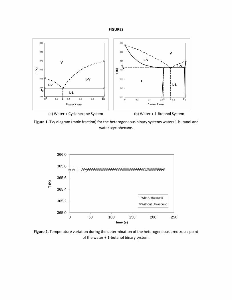
The isobaric Txy equilibrium diagrams of the two systems are shown in Figure 1, using the same

temperature scale. Both systems are heterogeneous and consequently any water-solvent

heterogeneous mixture boils at the azeotropic temperature (Tz). At that temperature, the global

mixture splits into two liquid phases of composition E and F in equilibrium with a vapor of

invariant composition Z. Obviously, the two liquid conjugated phases of the binary azeotrope of

the two systems have different properties; for instance, solubility, density and interfacial tension

are shown in Table 2 15–19. In this table are also found the boiling temperatures of the pure

substances and the heterogeneous azeotrope. The mutual solubilities water - cyclohexane are very

low and the composition of the two liquids in equilibrium in the azeotropic mixture is very

different. However, as the solubility of water in 1-butanol is large, the differences in the

composition of the two liquid phases of the azeotrope is smaller and consequently the difference

between the phase densities and the interfacial tension is smaller.

In order to illustrate the behavior of both systems during the determination of the LLV equilibrium

in the azeotropic point at 101.3 kPa, two experiments were carried out for the system with

cyclohexane and other two for the system with 1-butanol. The two experiments for each system

differed in the equipment used in the determination:

a) Commercial equipment as described previously with the usual agitation in the boiling flask due

to the heating and boiling of the mixture.

b) Commercial equipment as modified by Gomis et al. 20 with an ultrasonic homogenizer (Braun

Labsonic P with an operating frequency of 24 kHz) coupled to the boiling flask to increase the

agitation and the dispersion of the two liquid phases whose LLV equilibrium is to be determined.

For each one of the four experiments the pressure and temperature read by the apparatus were

recorded continuously, as was the vapor phase composition. It was assumed that these should

match the equilibrium values. Figures 2 and 3 illustrate the behavior of both systems during the

determination of the LLV equilibrium with and without the use of ultrasound. Figure 2 shows the

evolution of temperature versus time for the water + 1-butanol system using the same

temperature scale width (1 K) as in Figure 3, where the fluctuations of the system with

cyclohexane are represented. The behavior for the 1-butanol system with and without ultrasound

coincides. In addition, the experimental temperature was 365.73 K, which matches the literature

value 15,18.

The vapor composition of the binary azeotrope coincides with that reported in the literature, as

can be seen in Table 3. However, the standard deviation was slightly higher in the experiments

without the ultrasound homogenizer.

Figure 3 shows the evolution of temperature versus time for the water + cyclohexane binary. In

this case, the temperatures recorded during the experiment without ultrasound oscillated greatly.

The oscillations persisted throughout the experiment and, as a result, a steady state could not be

reached. Applying ultrasound to this kind of system attenuates the oscillations, which leads to

practically constant temperatures that coincide with their literature values 18,19.

Something similar occurred with the vapor composition of the binary azeotrope shown in Table 4.

Without the ultrasonic homogenizer the composition varied considerably, as the high standard

deviation suggests. The mean value of all the data analyzed is very different from literature values.

When ultrasound was used to disperse the sample, the fluctuation diminished, as the standard

deviation shows, and the mean value coincides with the literature values 18.

The above results show that systems that are easily dispersed (similar phase densities and low

interfacial tension) can be determined using only recirculation and the conventional agitation

provided by the equipment, as in the case of the water + 1-butanol system. For this reason, easily

dispersed systems can be determined with equipment based on this technique, as is the case with,

for example, the one developed by Iwakabe and Kosuge 21. In contrast, mixtures that are difficult

to homogenize, such as those containing cyclohexane (different phase densities and high

interfacial tension) do not attain equilibrium. Large pressure and temperature fluctuations occur

as a result of the poor dispersion of the heterogeneous mixture.

The above observations and conclusions were obtained for similar proportions of the two phases

in the boiling flask. In the case where there was much more aqueous than organic phase and no

ultrasound applied to the boiling flask, the same phenomena as described above were observed

but with larger deviations. When the dispersion in the boiling flask is poor, the organic phase in

the upper layer is practically the only phase that is recirculated.

All the difficulties described so far are due to insufficient dispersion of the mixture. With

ultrasound a good dispersion of the phases was achieved, which led to temperature and pressure

stabilization for all the systems studied regardless of their properties. The phase dispersion does

not directly affect the equilibrium but can influence the mass transfer rate between the two liquid

phases, which ultimately affects the rate at which equilibrium is reached.

In determinations using the conventional equipment of systems where the observed dispersion of

the liquid phases is low, the liquid mixture in the boiling flask splits cleanly into separate phases,

and a clearly visible interface is formed between them. This clean separation leads to the

formation of a small interfacial surface, through which only a low rate of mass transfer between

phases can occur. This prevents the system from attaining stability because of the processes taking

place there. Consider as an example the isobaric phase diagram for the binary mixture shown in

Figure 4. Suppose that at any given moment the heterogeneous binary mixture may be found in an

equilibrium state; that is, there are two liquid phases: compositions xE and xF, and a vapor phase,

composition xZ, at a temperature TZ. If heat continues to be supplied to the system, and it is

somehow able to remain at equilibrium, a vapor of composition xZ will form. It follows that neither

the temperature nor the compositions of the liquid phases will change as long as the global

composition of the liquid mixture stays between xE and xF. However, this is not the case in practice

where the system moves away from equilibrium as a result of the following sequence of processes

as well as the characteristics of the partly miscible system: the heating and evaporation of a small

amount of the organic-rich phase produces a vapor of composition xZ that is richer in W than is the

liquid organic phase. Consequently, the W content of the organic-rich phase is decreased. As a

result, the composition of the organic-rich liquid phase in Figure 4 shifts from F toward G and the

bubble temperature increases. This displacement is compensated by the W transfer to the

organic-rich liquid phase from the water-rich phase or from the bubbles of vapor coming from the

heating of the water-rich phase. Obviously, in the water-rich phase similar effects produce the

displacement of point E toward point H and a resultant increase in the bubble temperature. If the

mass transfer rate between phases is large enough the changes in the composition of the liquid

phases will be negligible and the bubble temperature will remain steady. But, if the phases split

into two well-defined layers, the contact surface between them is small. As a result, the rate of

mass interchange between the two phases is not large enough to maintain a state of equilibrium.

Comparing the water + 1-butanol and water + cyclohexane systems, whose equilibrium diagrams

are shown in Figure 1, the differences between the boiling temperatures of the pure compounds

and of the azeotrope are smaller for the water + 1-butanol system. Besides, the mutual solubility

of the pure components is high. Therefore, the liquid saturation curve between the pure

component and the liquid-phase azeotrope composition is not as steep as it is for the

water + cyclohexane system. In fact, in the middle of the diagram it can be observed how large

changes in the liquid composition imply only small temperature variations.

Another process that provokes instability, encountered when operating commercially available

equipment based on the Gillespie principle, is a poor recirculation effect resulting from the clean

separation between the liquid phases in the boiling flask. Since the phase of lower density always

floats on the top of the phase of higher density, the lighter phase accumulates in the recirculation

conduit and the mixing chamber. This could lead to the extreme situation where only a single

phase, the heavier one, is present in the boiling flask, resulting in a state very far from equilibrium.

When this situation arises, the phases mix only periodically, either by a sudden boiling of a small

portion of the aqueous phase or because the lighter phase accumulated in the recirculation

conduit occasionally flows back into the boiling flask. As a consequence, the composition and the

temperature of the recirculation stream change abruptly. This phenomenon, including the sudden

drop in temperature, can be explained using again the example of the binary mixture whose phase

diagram is shown in Figure 4. Referring to this phase diagram, the heavier phase in the boiling flask

and the lighter phase accumulated in the recirculation conduit, both very far from equilibrium,

may be represented by points G and H. If the phases were to mix, and the global composition of

the mixture were to remain between xE and xF, the system would tend to equilibrium, as

represented by points E, F and Z. Since the equilibrium state occurs at a much lower temperature

than both points G and H, only a sudden distillation would allow the system to attain the

equilibrium temperature and composition. Given that this process of mixing occurs only

periodically, the temperature oscillates continuously, as can be seen in the videos enclosed as

Supporting Information.

ULTRASOUND AND OTHER MODIFICATIONS OF THE APPARATUS FOR THE DETERMINATION OF

SLV AND SLLV EQUILIBRIA

The determination of the isobaric equilibrium at the boiling temperature when a solid is present

requires a great deal of stirring of the mixture in the boiling flask in order to increase the

dissolution/precipitation rate of the solid particles so that it does not take long to reach

equilibrium. The application of ultrasound is the ideal method of increasing agitation as well as of

decreasing the size of solid particles, thus increasing the mass transfer rate between the different

phases present.

Moreover, further modifications are needed for an accurate determination. The solubility of a

solid in a liquid phase depends on the solid, the mixture of solvents and the temperature. The

dependence of the solubility on temperature is an important variable to be considered. The

solubilities of some salts show a high dependence with the temperature, changing substantially

with only small variations in temperature. Most increase the solubility with temperature but

others decrease. Moreover, the rate of dissolution of a solid in a liquid phase is usually lower than

the rate of dissolution of a liquid or a vapor. In addition, a liquid phase containing a dissolved solid

can remain in a supersaturated state for a long time. All these factors make reaching the

equilibrium state more difficult.

Accordingly, when attempting to reach the equilibrium state in the presence of salt, the

temperature is a variable that must be controlled with precision in all parts of the apparatus.

When the solubility dependence of the salt with temperature is small, the still with two

recirculations (Gillespie principle) containing the ultrasonic probe could be used directly in the

determination of SLLV and SLV equilibria. But if the dependence of the solubility of the salt on

temperature is high, it is necessary to control the temperature of the return stream of the non-

vapor phases (which can contain one or two liquid phases and in some cases a solid in suspension)

to avoid possible precipitations of salt, which could clog and block the return conduit or the

sampling valve installed. Moreover, the concentration of dissolved salt in the samples taken in

these conduits would not correspond to the concentration of salt at equilibrium.

In addition, a related problem may appear when there is no control of the temperature of the

returning liquid phases. Salt precipitation implies that the salt concentration in the liquid phase

reaching the mixing chamber would differ from that of equilibrium. Consequently, to reattain the

equilibrium state in the boiling chamber + Cottrell pump area the salt would need to be dissolved

or precipitated again. As explained previously, these mass transfer steps are slower compared to

those in the LL and LV systems. The reaching of equilibrium would be hindered if the returning

liquid phases have their salt concentrations changed on their way to the mixing chamber.

In order to avoid these problems, several heating systems were installed around the returning

conduits, the sampling valve and the mixing chamber by including a controlled-heating electric

resistance around each one. The resistance maintained the temperature of these parts of the

equipment as close as possible to the equilibrium temperature of the mixture. With these

modifications the returning non-vapor phases at the exit of the Cottrell pump do not change their

salt concentration, aiding the reaching and maintaining of the equilibrium state, avoiding salt

precipitation that could block the equipment, and ensuring that the samples collected contained

the salt concentrations corresponding to equilibrium.

EQUILIBRIUM DATA FOR THE WATER + Na2SO4 OR K2SO4 + 2-METHYLPROPAN-2-OL SYSTEMS

By using the experimental apparatus with ultrasound and the modifications to maintain the

temperature of mixing chamber and the tubes connecting the different parts of the equipment

close to the boiling temperature, equilibrium data were determined for the water + Na2SO4 + 2-

methylpropan-2-ol and water + K2SO4 + 2-methylpropan-2-ol systems at 101.3 kPa and boiling

conditions. No SLV, LLV or SLLV equilibrium data have been found in the literature for these

systems under these conditions, although there are LL and SL equilibrium data for the system with

Na2SO4 at temperatures lower than boiling 22–24.

The data obtained for both systems are shown in Tables 5 and 6 and represented in Figures 5 and

6. These systems present, at boiling conditions, five different equilibrium regions: one LV region,

one LLV region, two SLV regions and one SLLV region. Both systems are able to split mixtures into

two liquid phases at boiling.

In both systems the data obtained follow the consistency rules when a salt is present 6: the boiling

isotherms on one side and the vapor iso-composition curves on the other side do not show

crossing points between the different parametric curves.

Comparing both systems, it can be seen that the size of the LLV region is noticeably larger in the

system containing Na2SO4. The range where the amount of K2SO4 is adequate to form two liquid

phases is lower than in for Na2SO4, and the amount of salt that can be dissolved is much lower.

With K2SO4, the aqueous phase of the SLLV region has only 1.4 mol % salt, while in the case of

Na2SO4, the same phase is formed by 5 mol % salt. This is in accordance with the fact that the

difference in composition of 2-methylpropan-2-ol between the aqueous and organic phases in the

SLLV region is lower in the case of potassium (0.013 and 0.324 respectively) than of sodium (0.001

and 0.486). The more ions there are in solution the higher the salting-out effect.

The extended UNIQUAC model for electrolytes 25 was used to calculate the equilibrium diagram of

each system. As an example, Figure 7 shows the results of one of them. It is important to point out

that the interaction parameters used25 had been estimated using only the SL and LL equilibria (but

not LV, LLV or SLLV equilibrium data) of the water + Na2SO4 + 2-methylpropan-2-ol system without

including data of the water + K2SO4 + 2-methylpropan-2-ol system, since there are no published

experimental equilibrium data for this system. The interaction parameters of 2-methylpropan-2-ol

with the K+ or SO42– ions were obtained from systems with containing these ions as other salts, i.e.,

KCl or Na2SO4. The application of these interaction parameters for the system with K2SO4 converts

the calculation in a prediction from the equilibrium of other systems. In spite of that, the results

calculated with the model are similar to the experiment, as shown in Figure 7 for the system with

K2SO4; the boiling temperatures and the shapes of the different regions are correctly predicted by

the model.

CONCLUSIONS

For the determination of LLVE data in systems with partly miscible compounds, it is important that

the two liquid phases are in intimate contact with each other. There are systems whose liquid

phases are easily dispersed as both phases have similar densities and low interfacial tension. These

systems can be determined using the conventional equipment for LV equilibrium determinations,

since dispersion and the mass transfer between liquid phases are easily obtained.

However, most systems with partly miscible components give two liquid phases with very different

phase densities and high interfacial tension; consequently, it is difficult for the mass transfer rate

between them to be high enough to attain equilibrium in a short time. Large pressure and

temperature fluctuations occur as a result of the poor dispersion of the heterogeneous mixture.

These systems require more sophisticated equipment because it is difficult to obtain good phase

dispersion of the liquid phases by mere agitation. In most cases, this type of systems could be

dispersed by coupling an ultrasonic homogenizer to the boiling flask of the equipment.

In the case of SLLV or SLV equilibria, the presence of salts makes reaching equilibrium and

maintaining the system in this state more difficult. The modifications to the equipment, comprised

mainly of the ultrasonic probe in the boiling chamber and the addition of a temperature control

system on the liquid return tube, help significantly in reaching the equilibrium state and avoiding

precipitation and/or dissolution of the salts.

The equipment with the aforementioned modifications permits to obtain accurate and consistent

equilibrium data when more than one solid or liquid phase apart from the vapor phase is present,

such as for the water + Na2SO4 or K2SO4 + 2-methylpropan-2-ol systems at 101.3 kPa and boiling

conditions. Comparing both systems, the size of the LLV region is larger in the system containing

Na2SO4. The determined experimental data of these systems were correctly predicted by the

extended UNIQUAC model for electrolytes, in spite of several interaction parameters having been

obtained without their experimental data.

Acknowledgment

The authors wish to thank Dr. Kaj Thomsen for his collaboration and help with the AQSOL software

used in the calculations. In addition, we would like to thank the DGICYT of Spain for the financial

support of project CTQ2014-59496.

Supporting Information

Four different videos are provided. The boiling flask, temperature and pressure in the apparatus

have been recorded in each video for different systems:

Two videos, (1-butanol without US.mp4) and (1-butanol with US.mp4), correspond to the system

water + 1-butanol without and with the ultrasound homogenizer: there are not large fluctuations

in temperature and pressure regardless of whether the ultrasound probe is connected or not

The other two videos, (cyclohexane without US.mp4) and (cyclohexane with US.mp4), correspond

to the binary water + cyclohexane system without and with ultrasounds: sudden boiling occurs

without ultrasounds, causing large fluctuations in pressure and temperature. When using the

ultrasound homogenizer, the fluctuations become smaller.

REFERENCES

[1] Gomis, V.; Pequenín, A.; Asensi, J.C. A review of the isobaric (vapor + liquid + liquid) equilibria

of multicomponent systems and the experimental methods used in their investigation. J. Chem.

Thermodynamics 2010, 42, 823–828.

[2] Garcia-Cano, J.; Gomis, V.; Asensi, J.C.; Gomis, A.; Font, A. Phase diagram of the vapor-liquid-

liquid-solid equilibrium of the water + NaCl + 1-propanol system at 101.3 kPa. J. Chem. Therm.

2018, 116, 352-362.

3) Younis, O.A.D.; Pritchard, D.W.; Anwar M.M. Experimental isobaric vapour–liquid–liquid equilibrium data for the quaternary systems water (1)–ethanol (2)–acetone (3)–n-butyl acetate (4) and water (1)–ethanol (2)–acetone (3)–methyl ethyl ketone (4) and their partially miscible-constituent ternaries. Fluid Phase Equilib. 2007, 251, 149–160.

4) Lee, L-S., Lin C-H. Phase Behaviors of Water + Acetic Acid + Methyl Acetate + p-Xylene Mixture

at 101.32 kPa. Open Thermodyn. J. 2008, 2, 44–52

5 Gomis, V.; Ruiz, F.; Asensi, J.C. The application of ultrasound in the determination of isobaric

vapour-liquid-liquid equilibrium data. Fluid Phase Equilib. 2000, 172, 245-259.

[6] Lladosa, E.; Montón, J.B.; Burguet, M.C.; de la Torre, J. Isobaric (vapour + liquid + liquid)

equilibrium data for (di-n-propyl ether + n-propyl alcohol + water) and (diisopropyl ether +

isopropyl alcohol + water) systems at 100 kPa. J. Chem. Therm. 2008, 40, 867-873.

[7] Pienaar, C.; Schwarz, C.E.; Knoetze, J.H.; Burger, A.J. Vapor–Liquid–Liquid Equilibria

Measurements for the Dehydration of Ethanol, Isopropanol, and n-Propanol via Azeotropic

Distillation Using DIPE and Isooctane as Entrainers. J. Chem. Eng. Data 2013, 58, 537-550.

[8] Garcia-Cano, J.; Gomis, A.; Font, A.; Saquete, M.D.; Gomis, V. Consistency of experimental data

in SLLV equilibrium of ternary systems with electrolyte. Application to the water + NaCl + 2-

propanol system at 101.3 kPa. J. Chem. Therm. 2018, 124, 79-89.

[9] Gomis, A.; Garcia-Cano, J.; Font, A.; Gomis, V. SLLE and SLLVE of the water + NH4Cl + 1-

propanol system at 101.3 kPa. Fluid Phase Equil. 2018, 465, 51-57.

[10] Gomis, A.; Garcia-Cano, J.; Asensi, J.C.; Gomis, V. Equilibrium Diagrams of Water + NaCl or KCl

+ 2-Methyl 2-Propanol at the Boiling Temperature and 101.3 kPa. J. Chem. Eng. Data 2018, 63,

4107-4113.

[11]Taboada, M. E.; Veliz, D. M.; Galleguillos, H. R.; Graber, T. A. Solubilities, Densities, Viscosities,

Electrical Conductivities, and Refractive Indices of Saturated Solutions of Potassium Sulfate in

Water + 1-Propanol at 298.15, 308.15, and 318.15 K. J. Chem. Eng. Data 2002, 47(5), 1193-1196.

[12] Iqbal, M.; Tao, Y.; Xie, S.; Zhu, Y.; Chen, D.; Wang, X.; Yuan, Z. Aqueous two-phase system (ATPS): an overview and advances in its applications”. Biological Procedures Online 2016, 18, 18.

13 Mangum, B.W.; Furukawa, G.T. U.S. Department of Commerce. National Institute of

Standards and Technology, Springfield, 1990.

[14] Hougen, O. A.; Watson, K. W.; Ragatz, R. A. Chemical Process Principles. Part I. 2nd edn. Wiley,

New York 1954.

15 Gomis, V.; Font, A.; Saquete, M.D.; Garcia-Cano, J. Liquid-liquid, vapor-liquid, and vapor-

liquid-liquid equilibrium data for the water-n-butanol-cyclohexane system at atmospheric

pressure: experimental determination and correlation. J. Chem. Eng. Data. 2013, 58, 3320-3326.

16 Poling, B.E.; Prausnitz, J.M.; O’Connell, J.P. The properties of gases and liquids. 5th Edition.

McGraw Hill. New York. 2001.

17 CHEMCAD VII, Process Flow Sheet Simulator, Chemstations Inc, Houston, 2016.

18 Gmehling, J.; Menken, J.; Krafczyk, J.; Fischer, K., Azeotropic Data, VCH, Weinheim, 1994.

[19]Liu, L.; Cheng, Ch.; Mu, X.; Li, H.; Tan, W. Isobaric vapor-liquid-liquid equilibrium for water +

cyclohexane + acetic acid at 101.3 kPa. Fluid Phase Equil. 2013, 350, 32-36.

20 Ruiz Bevia, F.; Gomis Yagües, V.; Asensi Stegman, J.C. Método y equipo para la determinación

del equilibrio liquido-liquido-vapor isobárico en sistemas heterogéneos. Spain. Patent ES 2 187 220

B2. December 1, 2003.

21 Iwakabe, K.; Kosuge, H. Isobaric vapor-liquid-liquid equilibria with a newly developed still.

Fluid Phase Equilib. 2001, 192, 171-186.

[22] Emons, H.H.; Röser, H. Das Verhalten von Natriumsulfat in Wasser-Alkohol-Gemischen.

Zeitschrift fuer Anorganische und Allgemeine Chemie 1966, 346, 225-233.

[23] Brenner, D.K.; Anderson, E.W.; Lynn, S.; Prausnitz, J.M. Liquid-liquid equilibria for saturated

aqueous solutions of sodium sulfate + 1-propanol, 2-propanol, or 2-methylpropan-2-ol. J. Chem.

Eng. Data 1992, 37, 419-422.

[24] Lynn, S.; Schiozer, A.L.; Jaecksch, W.L.; Cos, R.; Prausnitz, J.M. Recovery of anhydrous Na2SO4

from SO2-scrubbing liquour by extractive crystallization: liquid-liquid equilibria for acqueous

solutions of sodium carbonate, sulfate, and/or sulfite plus acetone, 2-propanol, or tert-butyl

alcohol. Ind. Eng. Chem. Res. 1996, 35, 4236-4245.

[25] Thomsen, K.; Iliuta, M.C.; Rasmussen, P. Extended UNIQUAC model for correlation and

prediction of vapor-liquid-liquid-solid equilibria in aqueous salt systems containing non-

electrolytes. Part B. Alcohol (ethanol, propanols, butanols)-water-salt systems. Chem. Eng. Sci.

2004, 59, 3631-3647.

TABLES

Table 1. Provenance table of the compounds used

Name CAS Provider Purity (weight fraction)

Water content (weight fraction)

Purification method

1-propanol 71-23-8 Merck >0.995 <0.001 none

1-butanol 71-36-3 Merck >0.995 <0.001 none

cyclohexane 110-82-7 Merck >0.995 <0.001 none

2-methylpropan-2-ol/ tert-butanol

75-65-0 VWR >0.999 <0.001 none

K2SO4/potassium sulfate 7778-80-5 VWR >0.997 none

Na2SO4/sodium sulfate 7757-82-6 Merck >0.99 none

Table 2. Boiling temperature of the pure compounds (Tb), phase composition (mole fraction) of

the binary azeotrope with water, boiling temperature of the azeotrope (Tb az), phase density and

the difference between them (), and the interfacial tension (). [15 - 19].

Component Tb16

Phase composition15

Tb az Density ( Tb az)17

(kg/m3) 17 16

(K) x1org x1

aq (K) org aq (kg/m3) (N/m)

1-Butanol 390.9 0.362 0.021 365.418-366.318 800.5 940.9 140.4 0.0015

Cyclohexane 353.9 0.997 0.0001 342.219-342.618 731.7 977.6 245.9 0.0497

Table 3. Vapor phase composition (mole fraction) and standard deviation of the heterogeneous azeotrope water + 1-butanol at 101.3 kPa and a boiling temperature of 365.7 K.

Bibliography

[18] Without

Ultrasound With

Ultrasound

x 1-butanol 0.250 0.251 0.250

Standard Deviation 0.027 0.011

The standard uncertainties of the boiling temperature and pressure are 0.06 K and 0.1 kPa respectively.

Table 4. Vapor phase composition (mole fraction) and standard deviation of the heterogeneous

azeotrope water + cyclohexane at 101.3 kPa and a boiling temperature of 342.4 K.

Bibliography

[18] Without

Ultrasound With

Ultrasound

x cyclohexane 0.701 0.557 0.698

Standard Deviation 0.258 0.036

When ultrasound is applied the standard uncertainties of the boiling temperature and pressure are 0.1 K

and 0.1 kPa respectively. When ultrasound is not applied the standard uncertainties of the boiling

temperature and pressure are 0.3 K and 3 kPa respectively

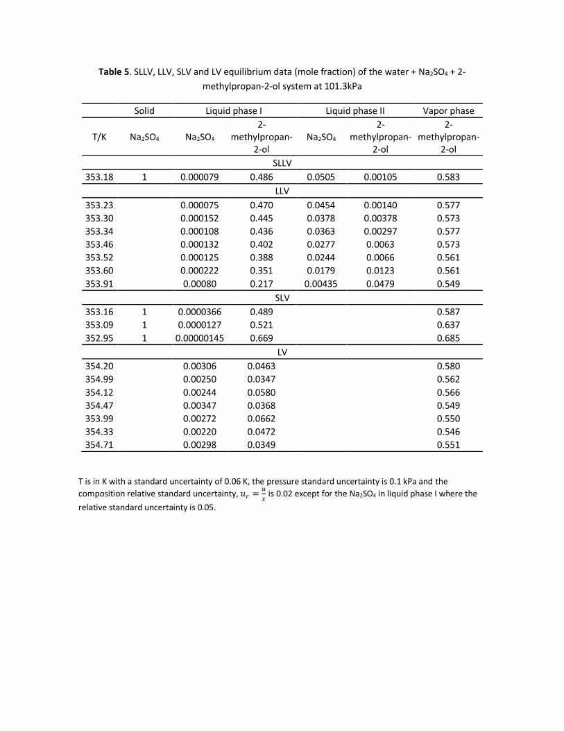
Table 5. SLLV, LLV, SLV and LV equilibrium data (mole fraction) of the water + Na2SO4 + 2-

methylpropan-2-ol system at 101.3kPa

Solid Liquid phase I Liquid phase II Vapor phase

T/K Na2SO4 Na2SO4 2-

methylpropan-2-ol

Na2SO4 2-

methylpropan-2-ol

2-methylpropan-

2-ol

SLLV

353.18 1 0.000079 0.486 0.0505 0.00105 0.583

LLV

353.23

0.000075 0.470 0.0454 0.00140 0.577

353.30

0.000152 0.445 0.0378 0.00378 0.573

353.34

0.000108 0.436 0.0363 0.00297 0.577

353.46

0.000132 0.402 0.0277 0.0063 0.573

353.52

0.000125 0.388 0.0244 0.0066 0.561

353.60

0.000222 0.351 0.0179 0.0123 0.561

353.91

0.00080 0.217 0.00435 0.0479 0.549

SLV

353.16 1 0.0000366 0.489

0.587

353.09 1 0.0000127 0.521

0.637

352.95 1 0.00000145 0.669

0.685

LV

354.20

0.00306 0.0463

0.580

354.99

0.00250 0.0347

0.562

354.12

0.00244 0.0580

0.566

354.47

0.00347 0.0368

0.549

353.99

0.00272 0.0662

0.550

354.33

0.00220 0.0472

0.546

354.71

0.00298 0.0349

0.551

T is in K with a standard uncertainty of 0.06 K, the pressure standard uncertainty is 0.1 kPa and the

composition relative standard uncertainty, 𝑢𝑟 =𝑢

𝑥 is 0.02 except for the Na2SO4 in liquid phase I where the

relative standard uncertainty is 0.05.

Table 6. SLLV, LLV, SLV and LV equilibrium data (mole fraction) of the water +K2SO4 + 2-

methylpropan-2-ol system at 101.3 kPa.

Solid Liquid phase I Liquid phase II Vapor phase

T/K K2SO4 K2SO4 2-

methylpropan-2-ol

K2SO4 2-

methylpropan-2-ol

2-methylpropan-

2-ol

SLLV

353.59 1 0.000215 0.324 0.0137 0.0131 0.560

LLV

353.62

0.000210 0.322 0.0135 0.0130 0.560

353.66

0.000298 0.303 0.0111 0.0165 0.560

353.69

0.000282 0.295 0.0102 0.0190 0.560

353.72

0.000322 0.281 0.0088 0.0217 0.559

353.75

0.000398 0.269 0.0077 0.0262 0.559

353.75

0.000343 0.257 0.0069 0.0298 0.559

353.79

0.00056 0.242 0.0058 0.0326 0.558

353.85

0.00078 0.221 0.00497 0.0387 0.558

353.90

0.00090 0.188 0.00350 0.0541 0.558

353.90

0.00117 0.152 0.00291 0.0602 0.555

353.90

0.00112 0.143 0.00253 0.0717 0.554

SLV

353.56 1 0.000166 0.335

0.569

353.42 1 0.000099 0.390

0.574

353.14 1 0.0000432 0.473

0.588

352.92 1 0.0000403 0.577

0.617

352.86 1 0.0000350 0.671

0.656

353.05 1 0.0000370 0.758

0.715

353.57 1 0.0000235 0.854

0.796

353.69 1 0.0000237 0.866

0.812

LV

356.92

0.0052 0.0106

0.502

359.11

0.00426 0.0074

0.473

362.59

0.0098 0.00248

0.395

358.26

0.00229 0.0109

0.484

356.86

0.0053 0.0111

0.510

357.71

0.0067 0.0084

0.499

355.02

0.000485 0.0294

0.545

354.39

0.00236 0.0292

0.545

353.96

0.00472 0.0259

0.554

T is in K with a standard uncertainty of 0.06 K, the pressure standard uncertainty is 0.1 kPa and the

composition relative standard uncertainty, 𝑢𝑟 =𝑢

𝑥 is 0.02 except for the K2SO4 where the relative standard

uncertainty is 0.05.

FIGURES

(a) Water + Cyclohexane System (b) Water + 1-Butanol System

Figure 1. Txy diagram (mole fraction) for the heterogeneous binary systems water+1-butanol and

water+cyclohexane.

Figure 2. Temperature variation during the determination of the heterogeneous azeotropic point

of the water + 1-butanol binary system.

333

343

353

363

373

383

393

0 0.2 0.4 0.6 0.8 1

T (

K)

x water, y water

V

L-V

L-V

L-LTZ

F Z E 333

343

353

363

373

383

393

0 0.2 0.4 0.6 0.8 1

T (

K)

x water, y water

V

L-V

L-V

L-LL

F EZ

TZ

365.0

365.2

365.4

365.6

365.8

366.0

0 50 100 150 200 250

T (

K)

time (s)

With Ultrasound

Without Ultrasound

Figure 3. Temperature variation during the determination of the heterogeneous azeotropic point

of the water + cyclohexane binary system.

Figure 4. Qualitative Txy diagram for a heterogeneous binary system.

342.0

342.2

342.4

342.6

342.8

343.0

0 50 100 150 200 250

T (

K)

time (s)

With Ultrasound

Without Ultrasound

F E

TZ

ZG H

T

xwater

V

L-V

L-V

L-L

L L

Figure 5. Equilibrium regions of the water + Na2SO4 +2-methylpropan-2-ol at boiling temperatures

and 101.3 kPa.

Figure 6. Equilibrium regions of the water + K2SO4 +2-methylpropan-2-ol at boiling temperatures

and 101.3 kPa.

Figure 7. Experimental and calculated equilibrium diagram for the water + K2SO4 +2-

methylpropan-2-ol at boiling temperatures and 101.3 kPa. Calculated regions by using the

modified UNIQUAC model 25.