S T U D I A G E O M O R P H O L O G I C A C A R P A T H O - B A L C A N I C A

VOL. XLV, 2011: 107–120 PL ISSN 0081-6434

WŁODZIMIERZ J. MOŚCICKI (KRAKÓW)

THE USE OF THE DC RESISTIVITY SOUNDING IN HIGH MOUNTAINS AREAS — EXAMPLE FROM PERIGLACIAL ZONE OF THE SUCHA WODA VALLEY (TATRA MTS., POLAND)

Abstract. In the paper selected problems connected with application of the DC resistivity sounding method in mountain geomorphology are discussed. The role of terrain topography is shown using numerical modelling. Pole-dipole DC resistivity sounding technique and interpretation and a case study from Hala Gąsienicowa in Polish Tatra Mts. are presented.

Key words: Tatra Mts., applied geophysics, DC Resistivity sounding, pole-dipole sounding, topo-graphic effects

INTRODUCTION

Geoelectric geophysical methods are nowadays widely used in geomorphologic studies (for example, S c h r o t t, S a s s 2008; H a u c k, K n e i s e l 2008). These are mainly resistivity methods. At early stage the DC resistivity sounding — VES — (K o e f o e d 1979) was dominant but lately electric resistivity tomography-ERT — (D a h l i n 1996) has gained more importance. These methods were mainly applied to non-invasive studies of permafrost in numerous mountain re-gions (for example, F i s c h et al.1977; K i n g 1984; E t z e l m ü l l e r et al. 2003; H a u c k, V o n d e r M ü h l l 2003; K n e i s e l 2004, S c a p o z z a et al. 2011, D o b i ń s k i et al. 1996, M o ś c i c k i, K ę d z i a 2001). Both methods have some limitations which should be taken into consideration during field works, data analysis and final interpretation. ERT method offers much better spatial recogni-tion (2D or even 3D) of the subsurface geology than DC sounding (1D). On the other side, the DC sounding has an advantage if the weight and portability of the equipment, ease of operation and costs are considered. The VES is especially useful when reconnaissance research is conducted (for example, recognition of the periglacial environment — B a u m g a r t-K o t a r b a et al. 2001, M o ś c i c k i et al. 2006).

108

DC RESISTIVITY SOUNDING IN THE PRESENCE OF NON-FLAT TOPOGRAPHY

Application of the VES in mountain environment encounters many difficulties. One type of a common problem is a non-flat surface of the terrain. Other prob-lems are connected with a subsurface geology which, if complicated, should be described in 2D/3D terms rather than with 1D model favourable for VES. As a re-sult, sounding curves may be disturbed in comparison to a typical curve shape. This makes standard quantitative 1D interpretation (K o e f o e d 1979) difficult and very limited. Usually, there is no a priori knowledge about the subsurface structures. However, terrain topography is visible, may be measured and thus may be taken into account. It means that it is possible to localize and perform VES in such a manner that effects from local topography (appearing as distur-bances of the sounding curve) are minimized. To do this the basic knowledge of the specific impact of topography on the VES is necessary. For quantitative estimation of the problem numerical modelling may be used (for example, M o ś c i c k i 2010). The knowledge gained from modelling may be used for bet-ter planning/performing VES and analyzing/interpreting field curves. Effective-ness of VES may be also improved if measurements are realized as pole-dipole or azimuthal pole-dipole sounding (for example, M o ś c i c k i, S o k o ł o w s k i 2009). In such a case horizontal changes in subsurface geology may be revealed and identified.

NON-FLAT TERRAIN MODEL

There may be dozens of models of topography describing mountainous terrain. Let us focus on one specific, simplified situation as an example: a 5 meter thick, uniform, sedimentary overburden lying on a flat basement rock. It could be scree, weathered material or glacial till lying on igneous rock, for example. The over-burden may have electric resistivity higher or lower than the basement. The flat surface of the model may have a depression or an elevation. This situation trans-lates to four geoelectric models presented in Fig. 1. The goal is to estimate the thickness of the overburden with a classic DC resistivity sounding method: four electrodes, symmetric Schlumberger array (AMNB). VES may be performed in a flat terrain or in a depression/elevation. Geoelectric models in Fig.1 were ana-lyzed with the use of RES2DMOD software (L o k e 2003) designed for the ERT method. From the huge set of apparent resistivites calculated for ERT some val-ues were extracted to construct “field” sounding curves (S1 and S4). These curves were first graphically compared with theoretical 2-layer curves i.e. curves for the ideal 1D, two-layer medium. Next, quantitative interpretation (inversion) was performed (IPI2WIN software — A. B o b a c h e v (2003); standard auto-matic interpretation) and results were compared with a true resistivity distribu-

109

tion (model). The correctness of interpretation is measured as a deviation be-tween “field” curve and theoretical curve, the latter one calculated for the inter-preted model (K o e f o e d 1979). This deviation is described by root mean square error (RMS, ε [%]). So-called equivalence phenomenon for the analyzed models is not discussed in the paper.

FLAT TERRAIN WITH DEPRESSION

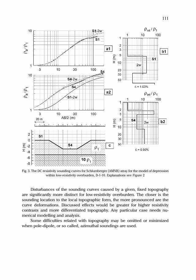
In the case of high-resistivity overburden (model D-10-1, Fig.1) disturbances of the sounding curves are slight — Fig. 2 a1 and a2. Interpreted models are very close to the real distribution of resistivity. Situation distinctly changes for high-resistivity basement (model D1-10) (Fig. 3). The S1 and S4 sounding curves are visibly deformed. The deformation occurs where the current electrodes are placed within the depression. Interpreted models (marked with thick lines in Fig. 3 b1 and b2) differ remarkably from real resistivity distribution (dashed line; 2w). Although the interpreted depth to the basement is not so far from the real one, the deeper distribution of resistivity may be misleading. It suggests the pres-ence of four different layers. In addition, the interpreted resistivity of the second layer is very high. Depending on the context of the survey it may be falsely iden-tified – as a sign of the permafrost presence, for example.

Fig.1. Simplified models of terrain topography. S1 and S4 — sounding points; ρ1 — electric resistivity

110

FLAT TERRAIN WITH ELEVATION

In that case the resistivity distribution plays, again, the most important role. For a low resistivity basement (in relation to the overburden) sounding curves show only slight disturbances — Fig. 4. The 1D inversion yields quite accurate resistiv-ity distribution from a practical point of view (the S4 case is slightly worse be-cause a false low-resistivity layer is “discovered”). For high resistivity basement the interpretation is much more complicated (Fig. 5). For S4 point the depth to the basement is estimated well. However, an additional low-resistivity layer ap-pears deeper, which is completely misleading.

Fig. 2. The DC resistivity sounding curves for symmetric, four-electrode Schlumberger (AMNB) array for the model of depression within high-resistivity overburden, D-10-1; Explanations: a1 — sounding curve in S1 site and its 1D interpretation — b1; a2 — sounding curve in S4 site and its 1D interpreta-tion — b2; c — 2D geoelectric model; symbols: ρa — calculated apparent resistivity, ρint — inter-

preted resistivity, ε — error of interpretation (r.m.s.)

111

Disturbances of the sounding curves caused by a given, fixed topography are significantly more distinct for low-resistivity overburden. The closer is the sounding location to the local topographic form, the more pronounced are the curve deformations. Discussed effects would be greater for higher resistivity contrasts and more differentiated topography. Any particular case needs nu-merical modelling and analysis.

Some difficulties related with topography may be omitted or minimized when pole-dipole, or so called, azimuthal soundings are used.

Fig. 3. The DC resistivity sounding curves for Schlumberger (AMNB) array for the model of depression within low-resistivity overburden, D-1-10. Explanations see Figure 2

112

Fig. 4. The DC resistivity sounding curves for Schlumberger (AMNB) array for the model of elevation on high-resistivity overburden, E-10-1. Explanations see Figure 2

POLE-DIPOLE SOUNDING

The DC resistivity sounding with pole-dipole (3-electrode) arrays were rather rarely used in geomorphology, mainly in permafrost studies (V o n d e r M ü h l l, S c h m i d 1993; L u g o n et al. 2004). The interpretation was used to be limited to 1D procedure, only.

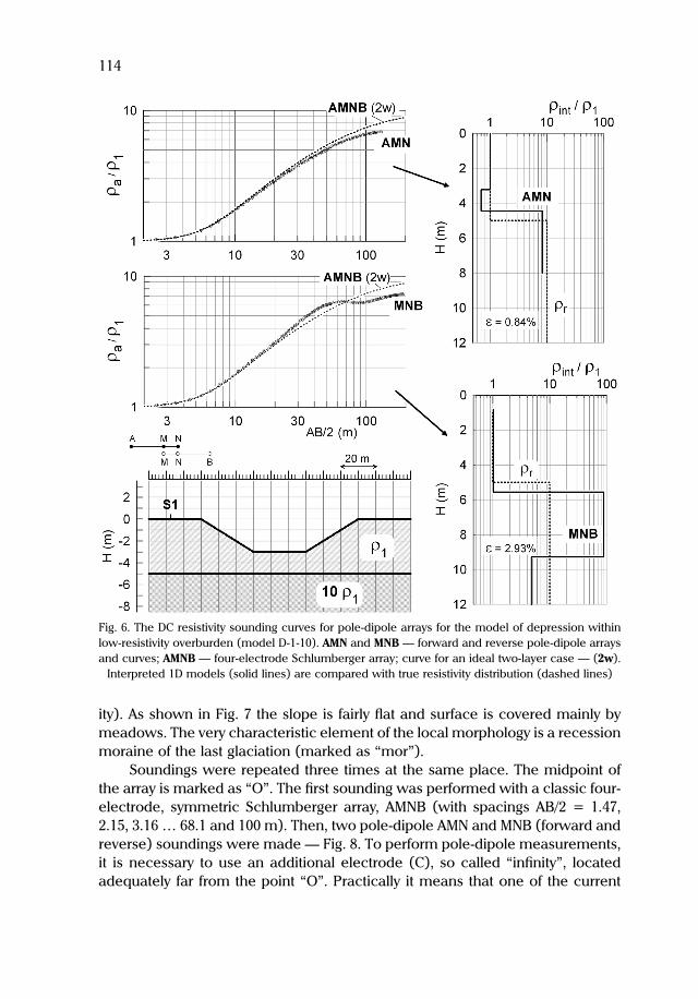
Let us examine advantages of a pole-dipole array over a classic four-elec-trode array. Let us consider the S1 sounding location: Model D-1-10 — Fig.1. The results of modelling and interpretation are presented in Fig. 6. The AMN variant recovers resistivity acceptably well. For the MNB case results are much worse and suffer from a relatively large error.

113

It is clear that specific topographic situation needs numerical analysis. Such an analysis enables to choose the most accurate location and direction of the pole-dipole sounding (direction of expanding array spacing).

DC RESISTIVITY SOUNDINGS ON THE NE SLOPE OF ŚWINICA PEAK

In this part of Hala Gąsienicowa area ground-temperature studies have been performed since 2004 (M o ś c i c k i 2008), aiming at finding permafrost occur-rences in the Polish Tatra Mts. (M o ś c i c k i, K ę d z i a 2001). The goal of geo-electric survey was a characterization of the site (layering — depth and resistiv-

Fig. 5. The DC resistivity sounding curves for Schlumberger (AMNB) array for the model of elevation on low-resistivity overburden, E-1-10. Explanations see Figure 2

114

ity). As shown in Fig. 7 the slope is fairly flat and surface is covered mainly by meadows. The very characteristic element of the local morphology is a recession moraine of the last glaciation (marked as “mor”).

Soundings were repeated three times at the same place. The midpoint of the array is marked as “O”. The first sounding was performed with a classic four-electrode, symmetric Schlumberger array, AMNB (with spacings AB/2 = 1.47, 2.15, 3.16 … 68.1 and 100 m). Then, two pole-dipole AMN and MNB (forward and reverse) soundings were made — Fig. 8. To perform pole-dipole measurements, it is necessary to use an additional electrode (C), so called “infinity”, located adequately far from the point “O”. Practically it means that one of the current

Fig. 6. The DC resistivity sounding curves for pole-dipole arrays for the model of depression within low-resistivity overburden (model D-1-10). AMN and MNB — forward and reverse pole-dipole arrays and curves; AMNB — four-electrode Schlumberger array; curve for an ideal two-layer case — (2w).

Interpreted 1D models (solid lines) are compared with true resistivity distribution (dashed lines)

115

electrodes, A or B, must be moved away to such a distance that remaining three electrodes (A, M and N or M, N and B) may be considered as a good pole-dipole array approximation. If the separation distance, OC = 10*OAmax or OC = 10*OBmax (what corresponds to 1000 m for AB/2max=100), in any direction, then pole-di-pole array differs from an ideal one only by 1%. Such a large separation may be difficult to obtain in mountainous terrain. The solution is to move C as far as possible and place it on a line which crosses the point “O” and which is perpen-

Fig. 7. Location of the soundings on NE slopes of the Świnica peak. a — general location of the study area, b — aerial photography of the area, c — composition of photographs made with standard 50 mm lens, d — view from the Karb pass (1853 m a.s.l.). Symbols: O — sounding site, Amax and Bmax — maximum of array spacing, C — location of the auxiliary electrode (“infinity”), mor — reces-sion moraine of the last glaciation. In ovals there are silhouettes of the measuring team members

116

dicular to the line joining potential electrodes MN. In such a case pole-dipole is ideal (from physical view-point), at least if isotropic half-space is considered.

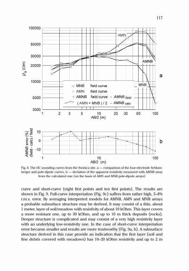
This idea was applied during field survey on Swinica (Fig. 7). Supporting electrode, C, was located on the northern side of the last glaciation recession moraine at a 100 m distance from the sounding point. The question is how good the pole-dipole array approximation was? This may be checked by comparing apparent resistivites measured with AMNB array with mean values calculated from measurements done with AMN and MNB arrays. The results are presented in Fig. 8. It is clear that AMNBfield and AMNBcalc curves are nearly identical and AMNBerror is quite acceptable. A bit higher error level for small spacings AB/2 is a result of the triple repetition of the measurements. In such a case it is not pos-sible to put electrodes in the exactly same places.

QUALITATIVE ANALYSIS OF THE SOUNDINGS

For a classic 1D model (uniform layers parallel to the flat surface) sounding curves for pole-dipole forward and reverse arrays and four-electrode Schlumberger are identical. In the case of Swinica study there is a dramatic difference in the shape of right branches of the pole-dipole curves — Fig. 8. At the beginning the AMN and MNB curves are similar (first seven points on the curves — to the spacing AB/2 = 14.7 m). Then, for larger spacings, apparent resistivity for AMN array raises rapidly, reaches 80 kOhm and more. It may be explained in at least two ways. Electrode A approaches to a very high resistivity obstacle or resistivity of the ground becomes higher and higher in this direction. At a distance of 70 m and more the sounding curve collapses — the electrode probably crosses the obstacle or leaves high resis-tivity zone. It should be pointed out that recorded resistivites are very high, and are much higher than typical values for igneous rocks. Therefore, resistivity values reaching some tens of kOhms may be considered as an effect of air-filled emp-ty spaces in the scree, or presence of permafrost. The last suggestion is less possible if the results of the ground temperature monitoring are taken into ac-count (M o ś c i c k i 2008).

Sounding curve for the BMN array behaves in a different manner. Measured apparent resistivites are less than 30 kOhm, and right branch of the curve rap-idly descends. In this case the electrode B reaches a low resistivity zone at 30–40 m spacing distance.

QUANTITATIVE INTERPRETATION OF THE SOUNDING CURVES

The 1D interpretation (K o e f o e d 1979) was used, although it is clear that a real field situation is rather 2D/3D, so interpretation results should be treated as a rough approximation. Interpretation was performed in several variants: full-

117

curve and short-curve (eight first points and ten first points). The results are shown in Fig. 9. Full-curve interpretation (Fig. 9c) suffers from rather high, 5–8% r.m.s. error. By averaging interpreted models for AMNB, AMN and MNB arrays a probable subsurface structure may be derived. It may consist of a thin, about 1 meter, layer of soil/meadow with resistivity of about 10 kOhm. This layer covers a more resistant one, up to 30 kOhm, and up to 10 m thick deposits (rocks). Deeper structure is complicated and may consist of a very high resistivity layer with an underlying low-resistivity one. In the case of short-curve interpretation error became smaller and results are more trustworthy (Fig. 9a, b). A subsurface structure derived in this case provide an indication that the first layer (soil and fine debris covered with meadows) has 10–20 kOhm resistivity and up to 2 m

Fig. 8. The DC sounding curves from the Swinica site. a — comparison of the four-electrode Schlum-berger and pole-dipole curves, b — deviation of the apparent resistivity measured with AMNB array

from the calculated one (on the basis of AMN and MNB pole-dipole arrays)

118

thickness. With increasing depth resistivity increases and geological medium becomes very heterogeneous. In the direction towards wall of Świnica (AMN up-sounding) very high resistivity objects/structures dominate while in the op-posite direction (MNB down-sounding) relatively low resistivites are observed.

Summarizing this research the following, near-to-surface geological struc-ture can be proposed. Under a relatively thin layer of soil, covered with meadows, there lies loose scree-type material, rather coarse-grained and blocky. Thickness of this layer may reach even 10 m. The amount of voids in this layer rises in the direction towards the wall of the Świnica peak. This may be a result of more intensive fine debris wash-out by the rainfall/snowmelt water flowing down from the wall and its NE couloir. The finest washed-out material is transported down the slope and may enrich deposits at the lower parts of the investigated slope. The same process may apply to a finer material coming from the neighbouring moraine. Interestingly, the ground in the sounding site is rather dry what suggests deeper paths of water drainage. As a result of the wash-out processes there may be a humid, fine-grained layer/zone of relatively low-resistivity forming at the

Fig. 9. Variants of quantitative 1D interpretation of the sounding curves from the Świnica site. AMNB — Schlumberger and AMN, MNB — pole-dipole arrays, a — field curves limited to AB/2max = 21.5 m, b — field curves limited to AB/2max = 48.3 m, c — field curves, full data — AB/2max = 100 m. Symbols: ρa — measured apparent resistivity, ρint — interpreted resistivity, ε — error of interpretation

(r.m.s.)

119

base of the slope. Simultaneously the upper part of the slope consists of coarser, blocky, well washed-out scree material. It should be remembered that topogra-phy of the basement (granite) rock determines the thickness of the loose sedi-ments and influences water flow paths, too. Perhaps, more knowledge about the basement topography could be gained with the electric resistivity tomography and/or georadar surveys.

CONCLUSIONS

The DC resistivity sounding curves are influenced by local terrain topography. The disturbance of the curve depends on the local topography form (elevation/depression) and on resistivity distribution. Topographic effects are stronger for low resistivity overburden lying on a higher resistivity basement. The distur-bances may lead to false geophysical and geomorphological interpretations. Application of pole-dipole soundings may help in such situations by lowering possible errors and enhancing geology recognition.

Application of pole-dipole soundings on NE slope of the Świnica peak re-vealed complicated structure of the near surface geology and intriguing resistiv-ity distribution.

The proposed and applied field technique shows that pole-dipole sounding may be used effectively and with acceptable accuracy even in a case of limited access to terrain.

The author is grateful to Professor Adam Kotarba for valuable comments. Thanks come also to Mariusz Krzak and Marcin Nowak who helped in the field work. I am thankful to Jakub Mościcki for discussions and help.

Financial support of this work from the fund of the AGH University of Science and Technology from project No.11.11.140.769 is kindly acknowledged.

AGH University of Science and Technology Faculty of Geology, Geophysics and Environmental Protection Department of Geophysics 30-019 Kraków, al. Mickiewicza 30 e-mail: moscicki@geol.agh.edu.pl

REFERENCES

B a u m g a r t - K o t a r b a M., K ę d z i a S., K o t a r b a A., M o ś c i c k i J., 2001. Geomorpholo-gical and Geophysical Studies in a Subarctic Environment of Karkevagge Valley, Abisko Moun-tains, Northern Sweden. Bulletin of the Polish Academy of Sciences, Earth Sciences 49, 2, 123–135.

B o b a c h e v A., 2003. IPI2WIN — Resistivity sounding interpretation, software. Version 3.0.1.a 7.01.03. Moscow State University.

120

D a h l i n T ., 1996. 2D resistivity surveying for environmental and engineering applications. FIRST BREAK 14, 7, 275–283.

D o b i ń s k i W., G ą d e k B., Ż o g a ł a B., 1996. Wyniki geoelektrycznych badań osadów czwar-torzędowych w piętrze alpejskim Tatr Wysokich. Przegląd Geologiczny 44, 259–260.

E t z e l m ü l l e r B., B e r t h l i n g I., Ø d e g a r d R., 2003. One-dimensional DC-resistivity depth soundings as a tool in permafrost investigations in high mountain areas of southern Norway. Zeitschrift für Geomorphologie, Supplementband 132, 19–36.

F i s c h W. S e n., F i s c h W. J u n., H a e b e r l i W., 1977. Electrical D.C. resistivity soundings with long profiles on rock glaciers and moraines in the Alps of Switzerland. Zeitschrift für Glet-scherkunde und Glaziologie 13, 239–260.

H a u c k C., K n e i s e l C., 2008. Applied geophysics in periglacial environments. Cambridge Uni-versity Press, Cambridge, 240 pp.

H a u c k C., V o n d e r M ü h l l D., 2003. Inversion and Interpretation of Two-dimensional Geoelect-rical Measurements for Detecting Permafrost in Montanious Regions. Permafrost and Periglacial Processes 17, 35–48.

K i n g L., 1984. Permafrost in Skandinavien — Untersuchungsergebnisse aus Lappland, Jotunheimen und Dovre/Rondane. Heidelberger Geographische Arbeiten 76, 177 pp.

K n e i s e l C., 2004. New Insights into Mountain Permafrost Occurrence and Characteristics in Glacier Forefields at High Altitude through the Application of 2D Resistivity Imaging. Permafrost and Periglacial Processes 15, 221–227.

K o e f o e d O., 1979. Geosounding principles, 1. Resistivity Sounding Measurements. Elsevier, Am-sterdam–Oxford–New York, 276 pp.

L o k e H., 2003. Rapid 2D Resistivity & IP Inversion using the least-squares method. Manual. Ge-otomo Software, Penang, 122 pp.

L u g o n R., D e l a y o l e R., S e r r a n o E., R e y n a r d E., L a m b i e l Ch., G o n z a l e s-T r u e b a J., 2004. Permafrost and Little Ice Age Glacier Relationships, Posets Massif, Central Pyrenees. Permafrost and Periglacial Processes 15, 207–220.

M o ś c i c k i W. J., 2008. Temperature regime on northern slopes of Hala Gąsienicowa in the Polish Tatra Mts and its relationship to permafrost. Studia Geomorphologica Carpatho-Balcanica 42, 23–40.

M o ś c i c k i W. J., 2010. Uwagi o stosowaniu geofizycznych metod geoelektrycznych w badaniach nieciągłej, wieloletniej zmarzliny górskie, [w:] A. Kotarba (ed.), Nauka a Zarządzanie obsza-rem Tatr i ich otoczeniem. t. 1, Nauki o Ziemi, TPN-PTPNoZ, Zakopane, 103-110.

M o ś c i c k i W. J., K ę d z i a S., 2001. Investigation of mountain permafrost in the Kozia Dolinka valley, Tatra Mountains, Poland. Norsk geografisk Tidsskrift 55, 1–6.

M o ś c i c k i W. J., K o t a r b a A., K ę d z i a S., 2006. Glacial erosion in the Abisko Mountains, Nor-thern Sweden. Geografiska Annaler 88 A (2), 151–173.

M o ś c i c k i W. J., S o k o ł o w s k i T., 2009. Electric resistivity and compactness of sediments in the vicinity of boreholes drilled in the year 2007–2008 in the area of Starunia palaeontological site (Carpathian region, Ukraine). Annales Societatis Geologorum Poloniae 79, 3, 343–355.

S c a p o z z a C ., L a m b i e l C ., B a r o n L ., M a r e s c o t L ., R e y n a r d E ., 2011. Internal structure and permafrost distribution in two alpine periglacial talus slopes, Valais, Swiss Alps. Geomophology 132, 208–221.

S c h r o t t L, S a s s O., 2008. Application of field geophysics in geomorphology: Advances and limi-tations exemplified by case studies. Geomorphology 93, 55–73.

V o n d e r M ü h l l D., S c h m i d W., 1993. Geophysical and Photgrammetrical Investigation of Rock Glacier I, Upper Engadin, Swiss Alps, [in:] Permafrost Sixth International Conference, Procee-dings. South China University of Technology Press, Beijing, 654–659.