The Use of Orthogonal Polynomial Contrasts in the · Blocking pattern due to confounding of (AeBe )...
117
• The Use of Orthogonal Polynomial Contrasts in the Confounding of Factorial Experiments by Dirk van der Reyden ,.' Institute of Statistics , { t Mime 0 Series No. 181 June, 19.5'1 r'
Transcript of The Use of Orthogonal Polynomial Contrasts in the · Blocking pattern due to confounding of (AeBe )...
•The Use of Orthogonal Polynomial Contrasts in the
Confounding of Factorial Experiments
by
Dirk van der Reyden
,.' Institute of Statistics,{
t Mime0 Series No. 181~""
June, 19.5'1
r'

TABLE OF CONTENTS
List of Tables
CHAPTER
iv
Page
vii
1
2
3
4
Introduction and Review of Literature
1.1 Introduction
1.2 Review of Literature
1.2.1 Symmetrical Factorial Design1.2.2 Asymmetrical Factorial Design1.2.3 Fractional Factorial Experiments1.2.4 Orthogonal Polynomials
1.3 Notation To Be Used
PART I. THE GENERAL CASE OF ORTHOGONAL OONrRASTS
Matrix Notation
1he Effects of Confounding a Single Contrast
3.1 Theorems
3.2 Bundles of Contrasts
The Effects of Confounding Two Contrasts Simultaneously
PART II. THE ORTHOGONAL POLYNOMIAL SYSTEM OF CONTRASTS
The Orthogonal Polynomials
5.1 Introduction
5.2 Partial and Complete Confounding
5.3 Partitioning of the Polynomial Values
5.4 Bundles of Homogeneous Order
1
1
5
79
1214
16
19
26
26
34
36
46
46
47
50
53

CHAPTER
v
Table of Contents (Continued)
Page
6 The Confounding Pattern of a Contrast
6.1 Bundles of Heterogeneous Order
6.1.1 Confounding on (AuBu.)6.102 Confounding on (AuBe )6.1.3 Confounding on (AeBe )6.104 Summary
56
56
56596162
6.2 Rules for Obtaining Confounding Patterns 64
6.2.1 Introduction 646.2.2 Polynomial Confounding Patters for
an m x n Experiment 656.2.3 A General Rule for Obtaining the Con-
founding Patterns of Any PolynomialContrast in an m x n Factorial Experiment 67
6.2.4 Polynomial Confounding Patterns for anm x n x p Experime~t 68
7
6.3 Determination of the Coefficients of theBlock Constants
The Confounding Pattern of Two Contrasts
7.1 Simultaneous Partitioning of Two OrthogonalPolynomials
70
73
73
7.2 The Generalized Interaction 75
7.3 Reduction Formulae for Products of OrthogonalPolynomials 76
7..4 The Status of the Contrasts in the LinearCombination 78
7 ..5 Confounding Patterns of Two Contrasts ConfoundedSimultaneously 79
8 Confounded ]OCperiments With Equal-sized Blocks
8..1 Confounding a Single Highest Order InteractionContrast
84
84

CHAPTER
8
vi
Table of Contents (Continued)
Page
(Continued)
8.2 Simultaneous Confounding of Two Highest OrderInteraction Contrasts
8.3 Experiments in Equal Blocks With Main EffectsUnconfounded
8.3.1 Two-factor Experiments8.3.2 Three-factor Experiments
89
94
9495
8.4 Confounding of Linear Combinations of Contrasts 99
8.5 Balanced Confounding 101
9 Summary, Conclusions and Suggestions for FurtherResearch
9.1 Summary and Conclusions
9.2 Further Research Needed
LITERATURE CITED
104
104
105
109

Table
1
2
3
4
5•
6a
6b
7
8a
8b
9
10
11
12
vii
LIST OF TABLES
Page
The orthogonal contrasts of the m x n x p factorialexperiment" 24
Conformable submatrices of (A B Ct ). 28r s
Signs of the conformable parts of (A B Ct)' (A~B Ch ),(A Be) r s r-g I.,
v Vi Z .. Lj...L
Signs and absolute values of the orthogonal polyriomials. 48
Numerical values of pl =AP • 49r r
Partitioning of the orthogonal polynomials. 52
Sums of elements of conformable parts. 53
Allocation of contrasts to homogeneous bundles. 55
Blocking pattern due to confounding of (.AuBu) whenm andn are odd. 57
Sums of elements of AE I(AuBu) (y = 1) correspondingto blocking pattern in Table 8a. 58
Blocking pattern due to confounding of (!nBe ) andcontrast totals. 60
Blocking pattern due to confounding of (AeBe ) andcontrast totals. 61
Confounding of general contrasts when specific ABcontrasts are confounded.. 63
General procedures for determining all confoundedcontrasts using polynomial confounding in a two-factor experiment. 66
13
14
15
16
Generalization of the parts of Table 12"
Confounding- pattern for any polynomial contrast inan m x n x p factorial experiment.
Confounding pa.tterns of the four basic contrasts ofhighest order of an m x n x p factorial experiment.
Products of polynomials"
68
69
77

'fable
17
18
19
20
21
22
24
List of 'fables (Continued)
Form of generalized interaction contrast.
Rule for obtaining homogeneous bundles in thegeneralized interaction of the contrasts (rs,fg) ofan m x n experiment
Examples of contrasts which satisfy condition (8.3),with at least two contrasts having zero elements.
Frequencies of block indicators in the orthogonalpolynomials.
Size of blocks when (.A:rBs,AfBg ) is confounded undercertain conditions.
Signs of the elements of the orthogonal polynomialvectors.
Confounding contrasts of highest order not confoundingmain effects and yielding four equal blocks when takenin pairs.
New three-factor experiments in four equal blocks withmain effects unconfounded.
viii
Page
78
82
86
88
90
93
97
99

Errata
The Use of Orthogonal Polynomial Contrasts in theConfounding of Factorial Experiments
Page 7, line 4: for sn/k read en/k.
Page 10, line 13: for electrotonic read electronic.
Page 16, line 13: for at read of.
Page 19, line 3 of second paragraph: for very read vary.
Page 23, third line from bottom: for (J~, J~)' read (J~, J~).
Page 25, line 1: for (J , J') read (JI, J').- + - +
Page 29, equation (3.2):
Page 30, equation (3.3):
read (A B Ct ) •r s +
read (A B Ct ) •r s +
for (tr b ) read (tr b ).e- -s-
for (A B Ct )r sfor (A B Ct )r s
(3.3.1), fourth line:Page 32, equation
Page 37, third line from bottom: for ar read a-+ r-+
Page 39, line 15: for were read where.
Page 43, first line of Theorem 4.1: delete T in (ArBsCtT,AfBgCh)'
Page 47, line 3: tor Pri read Ipril.
Page 48, N even, P3
: for 3(N2.4) read 13(N2-4)\ •
Page 50, third line from bottom: tor (p ,P , ••• ) read P2 P4 .,,)., ,Page 54, third line from bottom: for Hnece read Hence.
Page 57, title of Table 8a: for Blooking read Blocking.
Page 58, Table 8b, last column: tor sE read -sEao ao
Page 65, line 11: for othogonal read orthogonal.
Page 70, line 11: for J'a b c J read J'a b 0tJ.r ePage 89, line 6: for afibgj ) read (afibgj ).
Page 90, Table 21, fourth line: for n + n read n++ + n++ +-
Page 91, line 8: for Ph+ =Ph- read Ph+ =Ph.'
Page 92, equation (8.8): for (r - r ) read (n - n ).g+ g- g+ g-
Page 102, sixth line from bottom: tor A2B2Cl read A2B1Cl •

CHAPTER I
Introduction and Review of Literature
1.1 Introduction
Factorial experiments are used in experimental stiuations that
require the examination of the effects of varying two or more factorso
The various representatives of each factor are designated as levels, re~
gardless of whether they are continuous or discreteo In the complete
exploration of such a situation all combinations of the different factor
levels must be examined in order to elucidate the effect of each factor
and the possible ways in which each factor may be modified by the variation
of others.
When a factor is investigated at two levels, its main effect is
uniquely defined as the difference between the mean of the results at the
higher level and the mean of the results at the lower level. Its main
effect can thus be expressed as a unique contrast between the higher level
mean and the lower level mean. Interaction effects between two or more
factors, each at two levels, are also uniquely defined by similar con
trasts. Thus if, in a 23 factorial experiment, the factors are denoted
:1
w~ere the subscript 0 refers to the lower level, and if Yijk denotes the
response to the treatment combination aibjck' the contrasts can be pre
sented as follows:

2
Main
Response effects Interaction effectsA B C AB AC BC ABC
Yooo -1 -1 -1 +1 +1 +1 -1
-1 -1 +1 +1 -1 -1 +1YOOl
Y010-1 +1 -1 -1 +1 -1 +1
:r0 11 -1 +1 +1 -1 -1 +1 -1
Y100+1 -1 -1 -1 -1 +1 +1
Y101+1 -1 +1 -1 +1 -1 -1
Yuo+1 +1 -1 +1 -1 -1 -1
Y11l+1 +1 +1 +1 +1 +1 +1
It will be observed that any two of the contrasts are orthogonal;
ioeo, the sum of products of their corresponding coefficients is zeroo
This property of the contrasts makes for easy analysis, and ensures that
all the main effects and interactions can be independently estimated..
When the number of factors increases, the complete factorial design may
become too large to be accommodated under uniform experimental conditionso
The totality of treatment combinations is then subdivided into smaller
groups, each group being assigned to a given block of experimental units,
the grouping being made so that block effects will not affect the main
effects of the factors and those interactions regarded as being of impor-
tance 0 This process is termed "confounding 0 tl
Confounding of a contrast in the 2n series is accomplished by placing
these treatment combinations corresponding to the positive coefficients in
one block and those corresponding to the negative coefficients in another
blocko These parts of the contrast are now non-estimable from the data,

3
and we say that the contrast is completely confounded with block effects,
or in the usual parlance, with blocks ..
Even though the device of confounding may take care of the hetero
geneous material or conditions, with a large number of factors the total
. number of observations may become prohibitive.. Under certain conditions
it is then possible to examine the main effects of the factors and their
more important interactions in only a fraction of the number of treatment
oombinations required for the complete factorial experiment. This type of
design is known as a fractional factorial and is always equivalent to one
block in a system of confounding. In the 23 experiment, for instance, the
block containing the treatment combinations corresponding to either the
positive signs of ABC or to the negative signs of ABC would be a one-half
replicate ..
With factors at three or more levels, their main effects are no
longer uniquely expressible as contrasts between the different levels ..
It is well-known that the infinite number of contrasts that can be set up
between N observations can be divided into an infinite number of subsets
consisting of (N-l) orthogonal contrasts, with the property that the sum
of squares of each of the contrasts in the subset add up to the total sum
of squares of the observations, oorrected for the mean. In this thesis
exclusive attention will be paid to the subset of orthogonal contrasts
based on the orthogonal polynomial values tabulated by Fisher and Yates
(1938) and other authors.. Apart from satisfying the orthogonality oriteria,
these contrasts have usefUl interpretational value for an experiment in
volving factors with continuously varying levels; these being eqUally
spaced in the experiment.. The tables of the orthogonal polynomial values
have been set up in such a way that any value is either a positive whole
number, a negative whole number, or a 2rero ..

4
If a particular contrast is to be confounded with blocks and if it
contains no zero elements, a blocking procedure identical to the one for
the 2n experiment is applicable" If the contrast contains zero elements,
a third block is obtained by placing those treatment combinations corres
ponding to the zero elements in yet another bl9ck"
In general,\l when the number of levels exceed two,jl complete confound
ing does not occur with orthogonal polynomi8J... contrasts. Even though the
treatment combinations corresponding to the negative coefficients of, say
the linear contrast, are put in one block and those corresponding to the
positive coefficients are put in a second block, it is possible to esti
mate a linear contrast in each block based, of course, on only one half
the number of observations. These two estimates can then be pooled to
give a single estimate of the linear effect, adjusted for blocks. If
there are no block effects,Il the variance of the adjusted linear contrast
will be much larger than one not adjusted for blocks, because of the re
stricted range of the independent variable in each block" The actual
efficiency of the adjusted estimate will depend on the reduction of error
variance due to blocking.
A complete discussion of partial confounding in this sense should
include a method of estimating all pertinent contrasts and their standard
errors. This thesis, however,ll will be concerned only with the blocking
procedure5 •.
Although use has been made of orthogonal contrasts to obtain con
founded designs, in other than the 2n series,ll no systematic study appears
to have been made either on the theory of general orthogonal single con
trasts, or on the special system of orthogonal polynomial contrasts.
5
Whatever number of levels the factors may have, in many experimental
situations practical interest is mainly centered on the estimation of the
main effects and the lower order interaction contrasts, especially those of
second degree (linear x linear). One reason for this interest is the dif
ficulty of interpreting higher degree interaction contrasts. Most designs
appearing in the literature were developed from the point of view of ob
taining balanced sets of confounded blocks. It therefore appears to be of
interest to investigate the possibility of obtaining designs with the more
limited objective in mind. Considering the m x 19. x p experiment from this
point of view, one would be satisfied if a confounded design could be found
in which the main effects and most, if not all» of the linear by linear
interaction contrasts were unconfounded or only slightly confounded.
Simple a.nalyses and relatively precise estimates of these contrasts can be
obtained from a balanced set of replicates, but in many practical situa
tions the total number of observations thus required would be prohibitive.
With this background the objectives of this thesis may be summarized
as follOWS: (i) To investigate the theory of confounding general orthogonal
contrasts; (ii) to establish mathematical procedures and rules to obtain
the confounding patterns of higher order interaction contrasts, based on
the orthogonal polynomial system.
102 Review of Literature
Prior to 1926, when Fisher (1926) first suggested confounding, the
factorial experiment was known as the ueomplex tl experiment.; indeed, after
many years it was still referred to as the complex experiment. This type
of experiment had been used by the Rothamsted Experimental Station on
wheat experiments at Broadbalk since 1843 and on barley experiments at
Hoosfield since 1852; the randomization element, however, was lacking in

6
these early years 0 Fisher and Wishart (1930) gave a detailed explanation
of a confounded experiment, and Yates (1933) discussed the principles of
confounding, giving different types of confounding and setting out methods
of analysiso Later, Yates (1935) gave some more illustrations of confoundei'i
designs and discussed their relative efficiency compared with randomized
complete blocks o
Ever since the first appearance of the book liThe Design of Experi
ment n by Fisher (1935) and the monograph "The Design and Analysis of
Factorial Experiments" by Yates (1937), experimenters have used factorial
designs in a great variety of situations in many fields of researcho This
has led to a voluminous literature on all aspects of the subject. Mathe
matical statisticians became interested and found new explanations for
existing designs in terms of the results of combinatorial mathematics.
The utilization of these results, in turn, led to the development of new
designs. Special mention will be made of the work of Bose and his co
workers who gave the complete solution of the symmetrical factorial design.
Recently Binet et al (1955) re-examined most of the factorial plans
published to determine what effect the confounding had on the orthogonal
polynomial contrasts; in recent years these contrasts were found to be
important in certain fields of chemical and industrial researcho The
authors also presented new single-replicate plans, some of which were ob
tained by confounding of the higher order high degree orthogonal polynomial
contrasts. Anderson (1957) reviews the whole field of complete factorials,
confound and fractional factorials and explains the interrelationship of
these subjects 0 The present thesis is an attempt to formal ize some of
the techniques of Binet and his co-workers, and can hence be regarded as
providing the theoretical background for some of their practical findingso

7
1 0201. Symmetrical factorial designs
A factorial design is symmetric when each of the n factors is at s
levels, where s = pm and :£ is a prime number. Confounding occurs if each
complete replication is allocated to b =- sn/k blocks of ! plots each,
where ! divides sn 0 The problem that arises is how to allocate the treat-
ment combinations to the various blocks in such a way that only certain
desired treatment contrasts become non-estimab1eo Bose and Kishen (1940)
and Bose (1947, 1950) showed that by identifying the! levels with the
elements of a Galois field GF(pm), any treatment combination can be repre
sented by a point in finite Euclidean space EG(n, pm)o If any linear
homogeneous form U = aJ.X1. + aax2 + ••• + anxn is considered, where .the ! IS
belong to GF(pm) then U = c, where £ is a constant, will represent a flat
space of (n-1) dimensions. If the constant varies over all the elements,
U = c represents a pencil P(aJ.,aa, •• o, an) of parallel (n-l)-flats. To
each flat of the pencil corresponds a set of (n-l) treatment combinations,
and the contrasts between these ! sets carry (s-l) degrees of freedom •.
Thus the (sn_l ) degrees of freedom can be split into (sn_1 )/'(s_1) sets of
(s-l) degrees of freedom each, such that each set is carried by one parallel
pencil, and the degrees of freedom belonging to different sets are orth-
ogona10 If 1 particular coordinates of the penoi1 P(aJ.,a2,···,an ) are
nonzero, then the (.s-l) degrees of freedom carried by that pencil belong
to that particular (t-1)th order interaction. Thus if only one coordinate
of the pencil is nonzero, the (s-l) degrees of freedom will belong to that
particular main effect.
In practice these pencils can be obtained by means of the orthogonal
latin squares, since Bose (1938) showed that a latin square of prime order

8
can be regarded as the addition table of the roots of the cyclotomic poly
nomial, these roots being the elements 'of a Galois field.
It follows that when s=2, and the eXperiment:is confounded into two
equal blocks, a single contrast only will become nonestimable. When, how
ever, two contrasts of the 2n experiment are confounded, Barnard (1936)
showed that this implies the automatic confounding of another contrast, the
generalized interaction. He also gave various systems of confounding,
using factors up to 6 in number.
As far as symmetrical experiments are concerned, Yates (1937),
in his comprehensive monograph, gives designs, analyses and examples for
various confoundings of the 2n , 3D and 4n experiments. When s= 3, he
makes use of the combinatorial properties of the orthogonal latin squares
to define his orthogonal components 1. and:1., each with two degrees of free
dom. In terms of Bose's development these components correspond to the
pencils of parallel 2-flats. For s ::: 4, Yates derived confounded experi
ments by defining single degree of freedom contrasts, based on two pseudo
factors of two levels each, and blocking according to signs:",-similarly for
s = 8. He also suggested a routine of calculation for experiments with
several factors at two levels each, this depending only upon a succession
of additions and subtractions of pairs of numbers.
Nair (1938, 1940) discussed balanced confounded arrangements for
the 4n and :f experiments. Fisher (1942) established the connection be
tween the theory of finite Abelian groups and the relations recognizable
in the choice of interactions for confounding contrasts of the 2n experi
ment. He showed that, using blocks of 2r plots, it was possible to test
all combinations of as many as (2r -1) .factors in such a way that all inter
actions confounded shall involve not less than three factors each. He also

9
supplied a. catalog of systems of confounding available up to 15 factors,
each at two levels. Fisher (1945) generalized this proposition to factors
having s = pm levels, where E is a prime number.
Ke1'l'lpthorne (1947) introduced a new notation for the different
sets of degrees of freedom in the sn experiment to simplify the enumeration
and choice of systems of confounding. Comparing his notation with that of
Yates and Bose, we have, for instance, for the 32 experiment,. the following
components, each with two degrees of freedom:
Factor Yates Kempthorne Bose
A A A P(l,O)B B B P(O,l)
AB(I) AB P(l,l)AB AB(J) AB2 P(1,2)
Cochran and Cox (1950) survey the field of factorial experiments
mainly from an applied point of view, discuss detailed examples, give eom-
plete plans of those e~eriments most likely to be generally used in practice
together with details on the confounding and the relative information. In
his book Kempthorne (1952) devotes considerable space to a discussion of
the methods of confounding, the statistical models, methods of estimation
and the assumptions involved in the various confounded designs he presents.
Binet et al (1955) used the Bainbridge extension of Yates t (1937) technique
to examine the effects of the confounding systems proposed by the previous
authors on the orthogonal polynomial contrasts.
10202. Asymmetrical factorial designs
A factorial design is asymmetric when the ~ factors are respectively
Since G~lois fields do not exist for products of prime numbers, no single

10
mathematical system is available to deal with the confounding of the asym
metrical designo Of course, if the levels of a certain number of factors
are the same prime number or power of a prime number, the general theory
can be applied to that part of the experimento Thus in a 5 x 32 experi
ment the 32 part can be confounded as usual. In general, however, the
single replicates of such confounded designs are not very satisfactory
from a practical point of view, since low order interactions will be con
founded. This difficulty can be overcome by obtaining balanced sets of
replications, but such a procedure usually requires a triplication or more
of the total number of observations o
With a general mathematical theory lacking, much of the success in
obtaining satisfactory confounded designs will depend on the ingenuity of
the designero With the availability of electrotonic calculators, it is
conceivable thatgood practical designs may be obtained mechanicallyo
As far as asymmetric designs consisting of combinations of smaller
number of factors of 2, 3 and 4 levels are concerned, it would appear
that Yates (1937) and Li (1944) have supplied most of those likely to be
required in practice 0 The designs presented by these authors are balanced
with respect to the partial confounding of interactions, and more than one
replicate will usually be requiredo
When the number of levels of each factor is either 2, 4 or 89 Yates
(1937) employed the signs of contrasts with single degrees of freedom as
a basis for confounding o Consider the case of a factor A with four levelso
Since 4 :: 22, the factor A can be regarded as consisting of two pseudo
factors X and Y, each at two levels9 and hence the pseudo-effects are:

11
x :: (x-l)(y+l) = xy + x -y - (1)
Y :: (x+l)(y-l) :: xy.- x + Y (1)
XY :: (x-I) (y-l) :: xy - x - y + (1)
Let ao :: (1), a1. :: x, aa :: y:; a3
:: xy. Then
Ai :: a3
+ aa a1. ao:: Y
All :: a3 - aa a1. + ao :: XY
A"! = a3 - aa + a1. - ao
:: X
and it will be seen that
If the levels are equally spaced and if Al , Aa and A3 denote the linear,
quadratic and cubic orthogonal polynomial contrasts, then
~:: 2At -+ Alit
Aa :: A"
A3:: _Ai + 2AIII
For confounding purposes it should be noted that there is a one-to-one
correspondence between the signs of Ai and A1.' All and Alia' Alii and A3 •
Hence, since the confounding of any contrast proceeds on the basis of
the signs only, identical blocking arrangements will result with both
systems of contrastso
Employing Yates! techniques, Li (1944) constructed confounded
designs for 10 types of the asymmetrical factorial experiment with the
purpose of filling some of the gaps existing among the plans previously
available 0 Nair and Rao (1948) developed a set of sufficient combinatorial
conditions for the balanced confounded designs, and discussed the

12
requirements for optimum designs& Thompson and Dick (1950) showed how to
obtain factorial experiments in blocks of equal size, equal to or less
than the number of levels in the leading factor from the orthogonal latin
squares & Thompson (1952) presented the layouts and details of statistical
analysis for two and three-factor designs, the number of plots per block
in no case exceeding five.
Binet et al (1955) re-examined the asyrmnetric designs proposed by
Yates and Li for the effects of the confounding on the orthogonal poly
nomial contrasts. Detailed tables are presented, showing which orthogonal
polynomial contrasts are confounded, and the size of the coefficients of
the constants of the block contrasts appearing in the expected values of
the treatment contrastse Using either single orthogonal polynomial con
trasts of high order interaction, or the methods of Yates, as a basis for
confounding, they present new single-replicate designs with confounding
patterns & Their investigation is entirely of a practical nature. The
present thesis supplies the theory of confounding a single orthogonal
polynomial contrast and the simultaneous confounding of two or more poly
nomial contrasts.
le2.3 Fractional Factorial Experiments
Referring to the mathematical summary at the begi~ning of Seotion
le2.1, fractionalization of a factorial experiment wi~l occur when in
stead of taking all the £ blocks, we take only ~ blocks where ~ is less
than b. We then have a Bib fraction of a complete replicate. Bose
(1950) summarized the mathematical procedures to obtain fractions of
factorial experiments, when the number of levels is either a prime number
or a power of a prime number. He showed that contrasts are no longer
separately estimable, but that the sum of the contrasts belonging to any

13
complete alias set is estimable. He pointed out, however, that i£ all
contrasts o£ any alias set with the exception o£ one contrast are o£ su£
£iciently high order to be negligible, then this one contrast is estimable.
Bose and his co-workers have recently expanded the original theory and de
veloped a whole series o£ new designs; these are to be published by the
National Bureau o£ Standards.
Finney (1945) originally developed the principles o£ £ractional
replication with particular re£erence to the 2n and 3n £actorial experiments
in terms o£ £initeAbelian groups. Finney (1946) presented a popular ex
position o£ these ideas, together with some plans and examples; and Chinloy,
Innes and Finney (1953) gave an interesting example o£ the use o£ a one
third replicate o£ a 35 experiment on sugar cane manurin~. An interesting
generalization o£ Yates' (1937) routine o£ calculation was included in
this paper.
Plackett. and Burman (1946) discussed what they call optimum multi
£actorial experiments which Kempthorne (1947) showed to be £ractionally
replicated designs. In his book, Kempthorne (1952) treats the general
case o£ £ractional repl~cation, and describes a one-ninth replicate o£ a
36 design applied to measurements on the consistency o£ types o£ canned
rood. Brownlee, Kelly and Loraine (1948) enumerated subgroups suitable
£or high-order £ractional replication £or 2n designs o£ practical interest.
Davies and Hay (1950) gave special attention to the use o£ £ractional
£actorial designs in sequence with special re£erence to industrial ex
periments. Kitagawa and Mitome (1953) and Davies et al (1954) compiled
plans £or £ractional designs o£ the 2n and 3n series. Daniel (1956)
discussed £ractional replication in industrial research.

14
Box and his co-workers [see Box (1952, 1954), Box and Wilson (1951),
Box and Hunter (1954), Box and Youle (1955)] have recently opened new
fields in which complete and fractional factorial experiments are fruit-
fully employed. Their work is devoted to the problem of determining opti-
mal factor combinations in chemical and industrial research, and to describe
the response surface in the neighborhood of this optimum. These procedures
are sequential in nature and have been described and reviewed by Anderson
(1953) and Davies et al (1954).
No work, as such, haS been done on the fractionalization of the
asymmetrical factorial experiment.
1.2.4 Orthogonal polynomials
The orthogonal polynomials used in statistics are discrete cases of
the well-known Legendre polynomials in mathematics 0 The latter are usually
defined between the limits of -1 and 1 by the formula of Rodrigues
Using results from the finite calculus, one can show that the discrete
orthogonal polynomials for n observations between the limits a and b
can be written as
r thwhere D denotes the r advancing difference, and or is an arbitrary
constant.
The orthogonal polynomial systems proposed by various authors for
the equi-distant case differ only in the choice of the arbitrary constant
cr ' this choice being dependent on the purpose the author had in mind.

15
Tchebycheff (1859) first gave the theoretical basis of the orthogonal
polynomials of least squares" He treats the nonequidistant as well as the
equidistant case, and for the latter derived a reduction formula" Poincare
(1896) developed similar polynomials for the nonequidistant case. Gram
(1915) developed orthogonal polynomials for the purpose of smoothing em-
pirical curves" Jordan (1929, 1932) simplified Tchebychefffs methods for
practical a.pplication, presented tables and explained the method of suc-
cessive summation of the observa.tions. He chose the arbitrary constant in
such a way that SSP (x) = n, where SS denotes the sum of squares.r
In the system proposed by Esscher (1920) the value of c r was de-
termined by the convention that the coefficient of xr shall be unity.
In his later system Esscher (1930) chose the same convention as Jordan.
A similar choice of arbitrary constant was made by Lorenz (1931), who de-
veloped his system of orthogonal polynomials-by means of determinants.
Fisher (1921) derived the polynomials in which x is measured from
the mean and adopted the convention that the coefficient of xr shall be
unity" Allan (1930) derived the general expression of this polynomial.
In his studies on the regression integral, Fisher (1924) presented orthogo-
nal polynoIllials such that SSPr(x) equalled unity" Fisher and Yates (1938)
present standard tables of the polynomial values for ~ through 52, and
r through 5. Anderson and Houseman (1942) extended these tables to n
through 104. DeLury (1950) presents values and integrals of these
polynomials up to n = 26 for all degrees.
Aitken (1933), by deriving new forms for the orthogonal polynomials
showed in a remarkably lucid way the relationship between the theory of
interpolation and the theory of orthogonal polynomial curve fitting" The
choice of the arbitrary constant equal to unity results in obtaining

16
integers throughout the standard tables presented by Van der Reyden (1943).
for Eo through 52 and !. through 9. Pearson and Hartley (1954) reproduced
part of these tables in slightly modified form for Eo through 52 and I'
through 6.
Due to the arbitrary nature of the constant cr , it follows that if
the greatest common factor is removed from the numerical values of a poly
nomial in any system described above, the resulting figures would be
identical for all systems.
1.3 Notation To Be Used
A factor and contrast
a element of coefficient matrix of factor A
B factor and contrast
b element of coefficient matrix at factor B
C factor and contrast
c element of coefficient matrix of factor C
D diagonal matrix
E or e even
Fr vector of tr !r; FR vector of tr !a
f subscript of A contrast
Gs++ matrix of tr E.s ; GS matrix of tr E.sg subscript of B contrast
Ht vector of tr !:!.t; HT vector of tr !:!.T
h subscript of C contrast; polynomial coefficient, Section 5.1
I identity matrix
i level of factor A
J vector
j level of factor B

confounded
k level of factor C; polynomial coefficient, Section 501.
L linear combination
M Ipl
m number of levels of factor A
N total number of yields
n number of levels of factor B
o zero
P polynomial
p number of levels of factor C
Q N/2 or (N-1)/2
R subscript of A contrast
r subscript of A contrast; degree of polynomial
S subscript of B contrast
s subscript of B contrast
T subscript of C contrast
t subscript of C contrast
U or 'U odd
17
v
w
x
x
z
subscript of contrast A (generalized interaction)
subscript of contrast B (generalized interaction)
level of general treatment
times; I-X
yield
subscript of contrast C (generalized interaction)
sign a ; sign P • coefficient 1 Section 702r r~
sign b ; sign P • coefficient~ Section 702s r~
sign ct
sign af

f sign bg
"l.. sign ch
If =..(b
~ polynomial multiplier
18

19
PART I. THE GENERAL CASE OF ORTHOGONAL CONTRASTS
CHAPTER 2
Matrix Notation
Let y. Ok be the yield resulting from the applioation of the treatJ..J
thment oombinations oonsisting of the i level of the faotor A with m levels,
the jth level of the factor B with n levels, and the kth level of the
factor C with p levels.
Arrange these yields into a. (mnp x 1) oolumn veotor, in whioh the
Yijk are ordered in the following special manner: first put both the sub
scripts i and j equal to zero and very the subsoript k from 0 to (p-l) to
obtaiil p oombinations; then, keeping the subsoript i fixed at 0, vary the
subsoript j from 1 to (n-l) for each of the p variations of k; finally,
vary the subscript i from 1 to (m-l) for all variations of the subsoripts
j and k.. In transposed form the subscripts of the vector y will thus read
as
OOO,OOl,.··,OO(p-l); OlO,Oll, .... ,Ol(p-l); 020,021,··.,02(p-l); •• ·,O(n-l)O,
O(n-l)l, ••• ,O(n-l)(p-l); 100,101, ••• ,10(p-l); 110,111, ••• ,ll(p-l); 120,121,
••• ,12(p-l); ••• ,1(n-l)0,· •• ,l(n-l)(p-l); ••• , (m-l)(n-l)O, (m-l) (n-l)l, ••• ,
(m-l )(n-l )(p-l)
If I denotes the identity matrix, !'tr" the trace (the sum of the
diagonal elements), and SSa = np(a2 +a21+···+a2 1)' let a = a. (mnp x mnp)r ro r r,m- r r
be the diagonal matrix

a I(np x np)ro
1ar1I(np x np)
o
o
20
, r=1,2,··· ,m-l
a lI(np x np)r,m-
such that tr ar = 0, and tr araf = 0 when r 1= f and tr araf = SSar when
r = f. If D denotes a diagonal matrix, let
and
t,hen tr a = np(tr a ) and tr a a", will equal zero when r is not equal tor -r -r-J.
f, and will equal SSa when r equals f, where SSa = np (SSa ).-r r . -r
Let b = b (mnp x mnp) denote the diagonal matrixs s
bsoI(p x p)
b s1 I(p x p) o
1II
o
bsoI(p x p)
bs1I(p x p)
o
o
o
s=l 2··· (n..l), . , ,
obsoI(p x p)
bs1I(p x p) o
o
such that tr b = 0 and tr b b . will equal zero when s 1=' g,' but will equalssg
SSbs when s = g, where SSbs = mp(b~o+b~1+ ••• +b~,n_l). Let

21
Then tr b =mp(tr b ) and tr b b = 0 when s f g, but equal to SSb when5 -5 -s-g -s
5 = g where SSb = mp(SSb ).5 -8
If St. is the diagonal vector D(oto,ct1,···,Ct,p_l), let Ct denote
the diagonal matrix ct (mnp x mnp)
C-t
C =to
•
•
o, t = 1,2, .. ·, (p-l)
suohthat>t3:' ct = O. and tr ct ch equals zero when t f h, but equals SSct
when t = h, where SSct = mn(c:O+c~1+"·+C:,P_l) = mn(SS£~).
Let Jt be the (1 x ~p) row vector, Jt = (1,1,···,1). Then
and hence
Jt&rbsctafbgChJ = tr(ararbsbgCtCh)
= (tr !.r!f)(tr £~g)(t r .£..tE.h)
This expression will equal zero when one or more of the following is
true: r f f, B , g, t f h; or when either r = 0, or s = 0, or t = O. It
will equal (SSa )(SSb )(SSo.) when r = f, s = g, and t = h •. As a special. ...or -s -v
case, ao = bo = Co = I(mnp xmnp).
A contrast between the Yijk will be (ArBsCt ) = JtarbsctY' when not
all three r, s, t are simultaneously zero. This will be a contrast, since
if Yijk = 1 for all i,j,k then

22
In the above expression the notation (y :::: 1) is used rather than (Yijk ::: 1)
to simplify typography..
Define respectively
A ::: (A B C ) :::: J'a b coY'r roo r 0
B ::: (A B C ) ::: JiaobscoYs o s 0
and
Ct ::: (A B Ct ) ::: J'a b ctY,o 0 0 0
where r::: 1,2,""', (m-l); s ::: 1,2, ••• ,(n-l); and t ::: 1,2,···,(p-l) as con-
trasts of the main effects A,B,C; alternatively these contrasts could be
designated as contrasts of the zero order interaction.
Define respectively
(A B ) :::: (A B C ) ::: J1a bscoY'r s r s 0 r
(ArCt ) ::: (A B Ct ) ::: J1a boCtYr 0 r
and
(B Ct ) ::: (A B Ct ) ::: J1a b ctY;s 0 s 0 s
r,s,t having the same ranges as before, as contrasts of the two-factor
inter~ctions AB, AC, and BC; alternatively these could be designated as
contrasts of the first order interaction ..
Define
(A B Ct ) ::: J~a b ctY,r s .. r s
r,s,t having the same ranges as before, as the three-factor interaction
contrasts} alternatively these could be designated contrasts of the second
order interaction ..
23
At times these contrasts will be indicated only by their subscripts,
as for instance in Table 1. All these contrasts are orthogonal to each
other by virtue of the definitions of the coefficient matrices a,b,c. The
orthogonal contrasts of an m x n x p factorial experiment can be displayed
as in Table 10
The major purpose of this thesis is to investigate the consequences
of using incomplete blocks in such factorial experiments. When all treat-
ment combinations are not included in each block of experimental units,
certain of the treatment contrasts become confounded (mixed up) with block
oontrasts. If a given contrast is orthogonal to block contrasts, it is
said to be unconfounded. We will consider confounding systems based only
on the signs of the elements of a contrast (plus zero, if zero elements
occur). When any contrast in Table 1 is confounded, the problem arises to
determine the effect this confounding has on the other contrasts.
From a matrix point of view, confounding amounts to a process of
partitioning of matrices. Consider, for example, the main effect contrast
A = J1a bey, and assume that no zero elements occur in the diagonalr roo
of a. Arrange the coefficients of the matrix a and the correspondingr r
elements of y so that the first npm elements in the diagonal of a will- r
have negative signs and the next npm+ elements in the diagonal will have
positive signs. Let a denote the (npm x npm ) matrix of negative ele-r- --
menta, and ar + the (npm+ x npm+) matrix of positive elements" It is well-
known that when a matrix in a product of matrices is partitioned, the other
matrices have to be partitioned conformably in order that the product may
retain its meaning. Accordingly, let (J~, J~) I and (y~, y~) I denote the
conformable partitionings of the vectors JI and y, so that we can write
the contrast as

24
Table 1 0 The orthogonal contrasts of the m x n x p factorial experiment.
A
B
C
AB
AC
BC
ABC
Total
Contrast
~ = 100
·•Am-I = (m-1)00
~. = 010
·•Bn_1 = 0(n-1)0
CJ. = 001·Cp_1 = OO(p-l)
~J.BJ. - 110
J\Bn_1 = l(n-I)O•
~a~ = 210
·AaB 1 = 2(n-l)0• n-·0Am_IBJ. = (m-1)10•
Am-1Bn_l = (m-1)(n-1)0
AJ.CJ. = 101•·0Am_1Cp_1 = (m-1)0(p-l)
BJ.C:J. = 011•··Bn
_1Cp_1 0(n-1)(p-l)
A:J.~Cl - III0
1
1
1
1
1
1
1
1
1
1
1
1
1
1
1
1
1
1
mnp-1

25
ar-
Ar
o
:: A + Ar- r+
where A :: J-' a Y is the value of the contrast A in the block contain-r- - r- ~ r
ing those Y values corresponding to the negative values of ar and
A + :: J I a v+ is the value of the contrast A in the block containing ther . + r~ r
Y corresponding to the positive elements of a •r Placing Y :: 1, we have
Since
A (y :: 1) :: Jfa J = tr a f 0r- - r- - r-
Ar+(y :: 1) :: J~ar+J+ = tr ar + f 0
= 1) = tr a = np(tr a ) = 0,r -r
and since
it follows that
Since any contrast is of the form J1arbscty where either n?ne, or
one, or two of the subscripts r, s, t are zero, it follows that partition-
ing of anyone, or any two, or of all three of the matrices ar' bs ' ct
will require conformable partitioning of the other and y. The confounding
of any particular contrast will thus partition the coefficient matrix: of
every remaining contrast of the experiment, but this partitioning mayor
may not confound the remaining contrasts with block effectso Problems of
this type will now be investigatedo In succeeding chapters, r, s and t
will be used to denote specific contrasts and R, Sand T general contrasts.

26
CHAPTER 3
The Effects of Confounding a Single Contrast
3,,1 Theorems
Theorem 3010 The confounding of any contrast belonging to any lower order
interaction does not confound any contrast belonging to any higher order
interaction 0
Consider any contrast, (ARBSCT
)
Suppose we select any element of vector!T' say cTk' ioe", set p = 1 0
Then
Since this is true for all coefficients cTk' ~BSCT will remain a con
trast regardless of how the levels of C are assigned to each block"
Hence it is possible to confound on any C-contrast, say Ct9 because there
is a one-to-one correspondence between the elements of !t and !T"
Symbolically this may. be expressed as
The above result can be extended to confounding on any BC~contrast,
say BsCt , assuming all A-levels are assigned to each block. Symbolically
Hence

27
since there is a one-to-one correspondence between bSj and bSj and between
0tk and cTk• By permutation of the letters of the contrast (~BSCT)' the
above results follow immediately for all permutations; hence the theorem
is proven.
Theorem 3:2 ~ When m, u, p are even numbers and none of vectors er, ~_S' or
.2.t ~ontains zero elements, and when the vector.~ has the same number of posi
tive,as negative elements, then, when (A B Ct) is confounded, (AB ), A andr s r s rB will be uneonfounded.s- ..
Suppose that the first m coefficients of a are negative and the-r
next m+ are positive,; that the first n_ of Es are negative and the next n+
are positive.; and finally, that the first p_ of .2.t are negative and the
next p+ are positive. Then ar , bs ' and ct can be written as
ar = D(ar _, ar +);
bs = D(b ,b+,b , b +);s- s s- s
ct = D(ct_,ct+,···,ct_,ct +)
where D denotes a diagonal matrix and the elements of the above matrices
have orders that will now be explained.
Consider some negative element a . in the (npm x npm ) matrixrl - --
a " This element will occur successively np times on the diagonal.r-
Since
we can say that the element a . will first occur in n n successive posi-rl ~-
tions, then in n-p+ successive positions, then in n~_ successive positions
and finally in n~+ successive positions on the diagonal of ar _. The
positive elements of ar + will be similarly arranged on the diagonal. That
is, a can be regarded as a (4 x 4) diagonal matrix having submatricesr-

28
as diagonal elements, respectively with orders (m_ny_) 2, (m..ny+)2,
(m_n~_):a, (m_n+p+)2 e Likewise ar + can be regarded as a (4 x 4) diagonal
matrix with diagonal elements having as orders the same expressions as for
a ,but with m+ substituted for m e Consequently the matrix a can be re-~ - r
garded as the (8 x 8) diagonal matrix given in Table 2 0
Table 2.1 Oonformable submatrices of (AB Ct. ) .r s
Y' = (y' y' I y'. y' y' y' y'i y' )--" --+' -+-' -++' +-' +-+- ++-,. +++
a = D(a , a , a , a , ar+,ar +, a ar +)r r- r- r- r- r+'
b = D(b , b b b b b b bs +)S s- s-' s+' s+' B-' s-' s+'
ct= D(ct _, ct +' ct _, ct +' ct_,Ct +' ct _, ct +)
lrheorder of the 8 respective submatrices are(m n p )2, (m n-p~)2,(m..n+p_)2, (m_n+p+)2, (m+ny_)2, (m+ny+)2, (m+n:p:)2, (m+n:p+). -
Examining ct
in a similar way, it can be expressed as the (8 x 8)
matrix shown in Table 2. Arrange the elements of y in such a manner that
y can be regarded as an (8 x 1) vector, shown in Table 2, where for example
the subveetor y denotes the m_ny_ elements of y that correspond with
the m_ny_ diagonal elements of the product ar_bs_ct_o
Placing those yields that correspond with positive values of
(a b ct ) into one block, and those that correspond with negative values intor s
another block, the constituents of the respective blocks will be given by
,Block 1: (y' y' y' y')'+++' +--' .-+-' .-+
Block 2: (y~+_, yL+, y~++, Y~_)'
,To examine the confounding pattern for contrast (A B C
t) considerr s

29
Jfa b c J = [Jf abc J + Jt, abc J + Jt abc Jr s t --+ r- s- t+ --+ -+- r- s+ t- -+- +-- r+ s- t- +-
+ J~. abc J ]+ [J' abc J + J'_++ar_bs+ct+J_+++++ r+ s+ t+ +++ --- r- s- t- ---
say
where J_+ denotes J(m_ny+:x: 1) and where: (ArBsCt )+ indicates the value
of the contrast in the block containing the positive elements of (a b ct).. r s
Consider (A B )(1' = l)I(A B Ct )+, which is'the value of (A B ) whenr s r s . . . r s
Yijk = 1 in the positive block of the confounded contrast (ArBsCt ).
Let t = 0 in the first square bracket of (3.1). Then
(ArBs)(Y = 1)1 (ArBsCt ) = (tr !r_)(tr £s-)p+ + (tr !r_)(tr £s+)p-
... (tr !r... )(tr £s-)p- (3.2)
+ (tr !r+)(tr £s ... )p+ 000
When p_ = p..., (302) becomes
(ArBsHY = 1) \(ArBsCt )... = (tr !r- + tr !r+)(tr £s- + tr £s ... )p+
= (tr a )(tr b )P+ = 0-r -s
since (A B ) is a contrast. A similar result can be derived forr s
(ArBs)(Y = 1) in the negative block of ArBsCto

30
Consider the value of-the contrast A (y = 1) in the positive blockr
of A B Ct 0 Let s = 0 in (J. 2), thenr s
(Ar)(y = 1) I (ArBsC t ) = (tr !r)(p+n_ + p_n+)
.. (tr !r.. )(p_n_ + p+n+)
(A )(y = 1) I(A B Ct ) = (tr a + tr a +)np+ = (tr a )np+ = 0r r s.... -r- -r -r
Similarly
(B~)(y = 1) I(ArBsCt ).. = (tr .£s)(P+l'n_ + p_m+)
+ (tr E.s+)(p_l'n_ + P+ill+)
= 0 when P_ = P+
Hence the theorem is proved.
Corollary 3.2.1. The confounding of (A B Ct.) will not confound (1) thoser s
contrasts obtained from (ArBsCt ) by putting anyone of the subscripts r,s,t
equal to zero if the vector whose subscript is equated to zero has the same
number of positive as negative elements; (2) those contrasts obtained from
(A B Ct. ) by putting either r and s, or rand t, or s and t equal to zero,r sif either one of the two vectors whose subscripts are equated to zero has
the same number of positive as negative elements.
This corollary leads to the following practical situation: when
contrast (A B Ct.) is confounded, the folloWing contrasts will be unconr s
founded if the condition(s) given on the right is(are) satisfied.

31
(ArBs) when P_ = P+
(ArCt ) when n_ = n+
(BsCt ) when m_ = m+
Ar when either n_ = n+ or P_ = P",
Bs when either ~ = m+ or P_ = P+
Ct when either m_ = m+ or n_ = n+
These conditions lead to
Corollary 3.2.2. When each of the vectors !r' '£8' oSt, has the same number
of negative as posItive elements, the confounding of (ArBsCt ) will not
confound any lower order contrast obtained from (A B Ct· ) by placing eitherr s
one or two of the subscripts r,s,t equal to zero.
When the contrast (ArBsCt ) is confounded, and we would like to
know under what conditions the lower order contrasts with sUbscript(s)
identical to one (or two) of r,s,t is(are) confounded, the results of
Theorem 3.2 apply. This theorem, however, states nothing about the con-
founding or not of lower order contrasts with subscripts different from
r,s,t.Also Theorem 3.2 dealt only with even m,n,p.
To investigate these points, consider the confounding of contrast
(ArBf) of an m x n experiment. We consider a two-factor experiment to
simplify typography: with a three-factor experiment we would obtain 27
submatrices instead of the 9 in the present case. Partition the vector
!r into a negative part !r- with m_ elements in the diagonal, a positive
part a + with m+ elements, and a zero part a with m elements. Parti--r· -ro 0
tion the vector b into a negative part b with n elements, a positive-s -s--
part b + with n+ elements, and a zero part b with n elements.-8 -80 0

Placing those yields that correspond to posi-
32
As before, if the matrix ar is expressed in terms of the diagonal
matrices a , a +' a , the matrix b can be expressed in terms of ther- r ro s
diagonal matrices b , b +' b , conformable to the parts of a. The ele-. s- s so r
menta of y can then be arranged into submatrices conformable to the products
of the parts of a and b •r s
tive values of (a b ) into one block, those that correspond to negativer s
values into another block, and those that correspond to the zero values
into yet another block, the elements of the respective blocks will be as
follows:
Block 1: (y~+, y~- ) I
Block 2: (yl_, y' ).-+
Block 3: (Y~o' y~o' y~+, y~, yl ) I00
The values of (A B )(y = 1) in the respective blocks will be givenr s
by the expressions
(ArBs)+(y = 1) =
(ArBs)Jy = 1) =
(ArBs)o(y = 1) =
(tr !r+)(tr ~s+) + (tr !r)(tr ~s-)
(tr !r+)(tr ~s-) + (tr !r_)(tr ~s+)
(tr a+)(tr b ) + (tr a )(tr b )"""I' -so -r--so
+ (tr a )(tr b +) + (tr a )(tr b )"""I'O -s . """I'o s-
+ (tr a )(tr b )-ro -so
parts of a..... conformable to a ,a +' a ,and similarly for b.c •-ft. -r- -r -ro -u
= 0
Consider contrast (AaBS)\(ArBs ). Let !aI' !a2' !a3 denote the
The
values of (~BS)(Y = 1) in the three blocks of (ArBs) can be obtained
by substituting the parts of ~ Iar and bsl bs in (3.3.1).

33
(AaBS)(y = 1) \(ArBs )+ = (tr !R2)(tr E.s2) + (tr !Rl)(tr E.sl)
(~BS)(Y = 1) I(ArBs )_ =(tr !R2)(tr E.sl) + (tr !.J.U)(tr E.s2) (0302)
(~BS)(Y = 1) I(.ArBs)o = -(tr ~3)(tr .£s3) (for R,S,>l)
Next consider contrast (~)I(ArBs)oThevalues of ~(y = 1) in the
first two blocks of (A B ) can be obtained by letting S == 0 in (3.302);r s
for the zero block one must rework the relationship from (303.1).
(~)(y == 1) I(ArBs )+ = (tr ~2)n+ + (tr ~l)n_
(~)(y =1)1 (ArBs )_ = (tr !a2)n_ + (tr ~l)n+
(L. ) (y = 1) I(A B) == (n-n )(tr B..-.3
)-11 r s 0 0 -Ii
(BS)(y = 1)1 (ArBs )+ = (m+)(tr E.s2) + (m_)(tr E.sl),
(BS)(y = 1) I(ArBs )_ == (m+)(tr 12S1 ) + (m_)(tr £S2)
(BS)(y == 1)1 (ArBs)o == (m-mo)(tr E.s3)
Having the above relations, we can now prove the following theorems.
Theorem 3030 In an m x n experiment if contrast (ArBs) is confounded,
contrast (~BS) will also be confounded unless one or both of these situ
ati ons prevail:
(i) ~IAr or Bsl Bs or both are unconfounded
(ii) tr !a3 = 0 and tr E.sl = tr E.s2; or·
tr E.s3 = 0 and tr 2:Rl = tr !.R2"
It is easy to show that, if (i) or (ii) prevails, (~Bs)I(ArBs)
is uneonfounded" What happens if one of these conditions is not .f'ul-
filled? It is obvious that either tr !a3 or tr E.s3 must be zero in order
to have (~BS) unconfounded"

34
If tr !R3 =0, tr !Rl =-tr !R2' and
Unless (i) is fulfilled, so that tr !R2 = 0, or tr £Sl = tr £S2 = 0,
or (ii) is fulfilled so that tr £S2 = tr £Sl' (AaBS) I(ArBs) will be con
founded with blocks o
Corollary 3.3.1. If (ArBs) is confounded, contrast Aa will also be con
founded unless one or both of these situations prevail:
(i) !alAr is unconfounded
(ii) tr !a3 = 0 and n+ = n_.
A similar statement can be made for BS•
This corollary follows immediately from (3.3.3) and (3.3.4). One
can rephrase this corollary as follows:
Corollary 3.3.2. If ~\Ar is confounded, Aa\(ArBs ) will also be confounded
unless tr !a3 = 0 and n+ =~. Similarly if BS\Bs is confounded,
(BS)I(ArBs) will also be confounded unless tr £03 I: 0 and m+ = m_.
30 2 Bundles of Contrasts
In terms of Theorem 3.3 we may define a bundle of contrasts of
homogeneous order to be that set of contrasts with properties such that
when any single contrast belonging to the set is confounded, all other
contrasts belonging to the set will also be confounded. In other words,
in terms of confcunding, any contrast will always possess a homogeneous
bundle. A homogeneous bundle of a contrast (ArBsCt ) or (rst) will be in
dicated by [rst].

35
In terms of corollary 30301 we may define a bundle of heterogeneous
order to be that set of bundles of homogeneous orders with properties such
that whim any contrast belonging to the homogeneous bundle of highest order
is confounded, all other contrasts ,in the bundle of highest order and all
contrasts belonging to all the other homogeneous bundles in the set will
be confounded. In terms of confounding, any contrast of higher order will
always possess a heterogeneous bundle, but a main effect contrast cannot
possess a heterogeneous bundle.

CHAPTER 4
The Effects of Confounding Two Constrasts Simultaneousll
We now investigate the case when two contrasts are confounded s:i1nul-
t aneously• For the sake of simplicity of representation, we are assuming
that none of the contrastshas zero elements, otherwise 93::: 729 submatrices
will result from the conformable partitionings. In the present case the
more manageable number of 64 will occur. This assumption is one of eon-
venience only, and similar procedures and results will hold for contrasts
with zero elements.
Consider the two contrasts (A B Ct ) and (AfB Ch ) where at least one, r s g
of the following inequalities holds: r 'I f, s 'I g, t 'I h; and a contrast
(A B C ) derived from the two previous ones in the manner shown below.vwz
a ::: D(a I, arlI, ... , a I)r ro r,m-l
af ::: D(a.foI, aflI, •• 0, af 11),rn-a ::: D(a I, avlI, ....., a I) ::: arafv vo v,m-l
where I ::: I(np x np) and a .'" a .af ...V1. r~ ~
Originally the row vector at = (a. ,a l,···,a 1) has m negative-r ro r r ,m- - '_
elements followed by m. positive elements (m_ + m+ ::: m). Corresponding
to the m negative elements of aI, there are a certain number of negative- -r
and a certain number of positive elements of the row vector
~ ::: (af ,afl,···,af . 1)· Hence a' = (a ,a l,···,a 1) would consist-.L 0 ,m- '-'V vo v v,m-
of a sequence of alternating positive and negative elements. Let us
rearrange a' so that it has a single sequence of negative followed by a-vsingle sequence of positive elements; then rearrange a' and a1..
-r -.L

37
Accordingly !~ will have (m_+ + m+_) negative elements where there are
m elements of at which are the products of negative elements from at and-+ -v -r
positive elements from !f' and m+_ elements which are the products of posi-
tive elements from a' and negative elements from ar'. Similarly there· are-r -
+ m++) positive elements of !~o Hence the (!;)I(!~) row vector has a
and !f '" (+5,-1,-4,-4,-1,+5).
at '" (-25,+3,+4,-4,-3,+25).-r
sequence of m_+ negative elements, m+_ positive elements, m negative
elements, and finally m++ positive elements. [If there were zero elements
in at and aft, there would be (m + m + m + m + + m ) zero elements-r - -0 +0 0- 0 00 .
in !~.] Similarly (~f)I(:.~) has a sequence of m_+ positive elements,
m+_ negative elements, m__ negative elements, and finally m++ positive
elements.. It is important to remember that the first subscript refers to
the Ar contrast and the second to the Af contrast. Extensions to more than
two contrasts can be made without too much difficulty.
As an example, consider the two row vectors a' '" (-5,-3,-1,+1,+3,+5)-r
Before rearrangement, the vector at will be-vAfter rearrangement we have the following
a' '" (-25,-4,-3,+3,+4,+25)-v
a ll '" ( +5,-4,-1,-1,-4, +5)-fat '" ( -5,+1,+3,-3,-1, +5)-r
In the diagonal matrices each element of the vector is repeated
•np times .. The matrices, rearranged according to a , are indicated asv
a la '" D(ar ~,a + a ,a + )r v -~ r -, r-- r +
aflav '" D(af_+,af+_,af__ ,af ++)
a /a '" D(a a a a )v .V v-+' v+-' v--' v++

38
where the first sign in the subscripts refers to the element in a , ther \
second sign to the element in af , and the sign in av is the product of the
two basic signs. The respective orders of the diagonal submatrices are
(npm_+ x npm_+), (npm+_ x npm+_), (npm_ x npm__ ), (npm++ x npm++).
A similar procedure can be followed for the B-contrasts and the
C-contrasts. As seen in the original definition of b ,we need consider8
only one of the submatrices here and then repeat the rearranged submatrix
m times to form the rearranged b matrix. Let us consider one of these
submatrices b(np x np). The two basic submatrices will be designated as
b~ and b;, and their product as b~. Hence
b·lb·s w
b"lb·g w
b¥-Ib.w w
= D(b· +,b.+ ,b* ,b·++)s-· s - s- s
= D(b~ +' b fIo+ , b- , b'lll++)g- g - g-- g
= D(b:_+,b;+_,b';_,b:++)
where the first sign in the subscripts refers to the element in b'lll and thes
second sign to the element in b"', and the sign in b* is the product of theg . w
two basic signs. The respective orders of the diagonal matrices are
(pn_+ x pn_+), (pn+_ x pn+_), (pn__ x pn__ ) and (pn++ x pn++). The cor
responding b-matrices are simply D(b" , b"" , 0 0 0 , b"') where b'f is repeated
m times.
In the c-matrices we need study only the diagonalized c-vector
c·(p x p) = D(Cto,Ctl,···,Ct,p_l). We will consider the two basic matrices
ct and c: with product c: 0
clltle.....t z
c.. \ c*h Z
c*IClf.Z Z
= D(ct_+"c!+_,ct_,ct....,)
= D(c~_+,c~+_,ct_,c~++)
= D(c:_+,c:+_,c:__,ci++)

39
where the signs in the subscripts have the same meaning as before, and the
respective orders of the diagonal matrices are (p_+ x p_+), (P+_ x P+_),
(p__ X P_ ), and (p++ x p++) • The corresponding c-matrices are simply
D( " lj!r *') . 't . dc ,e , ••• ,e where e :LS repeate nm times.
Sinee we have the relations
m =: m + m + m + m..L.L_+ +_ "'-T
n =: n_+ .... n+_ ... n ... n++
p=:p +p +p +p-+ +- -- . ++
where each subscript (~,~, ••• ,~) is either - or +. Hence there will be
64 terms in the sum. The elements of the y matrix can now be arranged
into 64 subvectors conformable to the products of the parts of
Thus
Y "" (y i Y i ; y' • •• Y i ) i. '-+-+~+'-+-++-' ~O~t~~' , ++++++
were the subvector y~o~~'t1\j.has m~6n~~'p~"l. columns.
Observe again that the first subscript of m or n or p (i.e., ~ or
~ or~) indicates the sign of the a or the b or the ct
in the relevantr s
part, and hence the product (~~r) will indicate the signs of the elements
of the contrast (ArBsOt ) in that part. The second subscript of m or n or
p (i.eo, 0 or e or~) indicates the sing of the af or the bg or the ch in
the same part as before, and hence the products (S~~ will indicate the
signs of the elements of the contrast (AfBgCh ) in that part. The products
lD "" ~6 or "'t. ::,!t or " =: 1"1. indicate the sign of a or b or c in the1" v w z
same part as before, and hence the products 'f"X..'Y "" ~6~tn will indicate the
signs of the elements of the contrast (A B C ) in that part.vwz

40
The sequence ..<, b, 'of, 13, to, 'X., 0 , "'l ' 'fI is thus the key to the study
of the confounding situation o When all those elements of y which have"
positive signs in (ArBsCt ) and (AfBgCh ) are placed in one block, those which
have positive signs in (ArBsCt ) but negative signs in (AfBgCh ) in another
block, those which have negative signs in (ArBsCt ) but positive signs in
(AfBgCh ) in yet another block, and those which have negative signs in both
(ArBsCt ) and (AfBgCh ) in the final block, then we will obtain the blocking
arrangement due to the simultaneous confounding of the two contrasts.
Table 30supplies the 64 possible combinations of the sequence; it
can be seen at once that if (A B Ct ) and (AfB Ch ) are confounded simul-r s g
taneously, (A Be) will be confounded automatically 0 (A B C ) can bevwz vwz
termed the generalized interaction of (ArBsCt ) and (AfBgCh ) and written
symbolica.lly as
(A B C ) ~ (A B Ct) x (AfB Ch )vwz rs· g
When, e.g., f ~ 0, s ~ 0, h = 0, (A BC ) ~ (A Ct) x B = (A B Ct) thevw z r. g r g
well-known Uinteraction l1 of (A Ct ) with B. It should be emphasized that. r -g
(A B C ) is a contrast, but in its generalized form will not be orthogonalvwz .
to all of the basic contrasts in the experiment.
Let (ArBsCt , A:rBgCh) denote the simultaneous confounding of the con
trasts within the brackets. Then
(ArBsOt)(Y =1)1 (ArBsOt.,A-.RgOh) = Jfa ~b c J.".r r..<u s j3f. tit
where the sum contains 64 terms. Similar expressions hold for (AfBgOh )
and (A B ° )when (A B Ct ) and (AfBCh ) are simultaneously confounded.v w z r s . g
Let (ArBsCt,AfBgCh)++ denote the block obtained by selecting those
treatment combinations that have a positive sign in A B Ct. as well as inr s

41
Sign of
+ 01- + + 01- + + + + (+) (+) (+) 01- - - + + + + + + ++ + + + + + + + + - - + + + - - -+ - -++ + + + + + + ... + - - +- +- + -+ - - (+) (+-) (+)+ +- + + + + - + - + + - - + + + - + - - ++ + + - - + + + + + + - - - - + + + + - ++ + + - - + + (+) (+) (+) + - - - - + - - + ++ + -+ ... + -+ + - - - - + + _. - - ++ + + - - + - + - + - -+ - - + - + - (+) (+) (+)+ + + + + + + + - + - - + - - + + + (+) (+) (+)+ -+ + + - - - + + + - - + - - - - + - ++ + + + - - + (+) (+ ) (+) + - - + - - + - -. -++ + + 01- - - - + - + + - - + - - - + - - ++ + + - + - + + + + + - - - + - + + -+ - ++ + + - + - - + + + - - - + - - - -+ (+) (+) (+)+ + + - + - + + + - - - + - + - - - -++ + + - + - - + - (+) ( +) (+) -+ - - - + - - + - +
+ + + + + + + ... - + - + + + + + -+ - +-+ -+ -+ + -+ (+) (+) (+) - -+ - + + + - - -+ -++ + -+ + + - + + - + + ... -+ - - - ++ + + + - ... - -+ + - + + + - + - (+) (+) (+ )
- - + - - + + + + (+) (+) (-+) - + - - - + -+ -+ -+ ...+ "" -+ -+ - + - - - -+ - - -+ - ...+ - - + "" ... -+ - - - ... ... - - (-+) (... ) (-+)-+ - - + - -+ - + + - - - -+ - -+ - - -+
- - + + -+ + + + - - + - + - - -+ + ... - -++ + - - + + + - + - - - - -+ (+) (+) (+)+ + - - + "" - + - + - - + - - - ++ + - + - (+) (+) (+) - + - + - - - + - ++ - + - + + + + - - + - - + - + + + (+) (+) (+)+ - + - + ... - - + - - + - - - + - ++ - + - + (+) (+) (+) - + - - + - + - - ++ - + + - + - + - - + - - + - - +
( ) indicates parts of (++) b1ocko
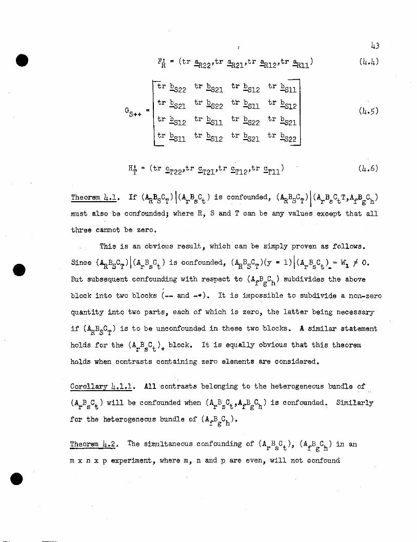
If F~ denote the (1 x 4) row vector (tr !r++,tr !r+_,tr !r_+,tr !r--)
and G the (4 x 4) matrixS't+

42
tr b tr b tr b tr b-s++ -s+- -s-+ -s--
tr b tr b tr b tr bG -s+- -s++ -s-- -s-+=s++
tr b tr b tr b tr b-s-+ -s-- -s++ -s+-
tr b tr b tr b tr b-s-- -s-+ -s+- -s++
and Ht, the (1 x 4) row vector (tr .£.t++,tr '£'t+_,tr .£.t_+,tr -St__ ),then, using
Table 3 to select those treatment combinations that have a positive sign in
(4.2)
Similar expressions hold for (AfBgCh)(Y = 1) and (AvBwCz)(Y = 1) in the
(++) block. To derive the value of contrast (~BSCT)(Y = 1) in that block,
let ~22 denote the part of !R conformable to ~r++ and afT"'; i.e., those
elements of !a for which the corresponding elements in both ~r and ~f are
positive. Similarly ~R12 denotes a vector for which the corresponding ele
ments of ~r are negative and of ~f are positive, etc. Similarly for the
parts of Es and.£.To Since
!It = ~ll + !It12 + ~21 + ~22
= !Rl' + ~2o
=~ol + !R.2
with similar results for £s and .£.T' we have a symbolic one-to-one corres
pondence between (ARBSCT) and (ArBsCt ) if 1 in the subscript of a vector
of the former is substituted for - in the latter and 2 for +. Hence
where
43
(4.4)
tr E.s22
tr E.s2l
tr E.s12
tr E.sll
tr E.s21
tr £022
tr E.sll
tr E.s12
tr E.s12
tr £011
tr £022
tr E.s21
tr E.sll
tr £012
tr E.s21
tr E.s22
(4.6)
Theorem 4.1. If (~BsCT)I(ArBsCt) is confounded, (AaBsCT)\(ArBsCtT,AfBgCh)
must also be confounded; where R, S and T can be any values except that all
three cannot be zero.
This is an obvious result, which can be simply proven as follows.
Since (~BsCT)I(ArBsCt) is confounded, (~BSCT)(Y = 1)\ (ArBsCt )_ = WJ. "I 0 0
But subsequent confounding with respect to (AfBgCh ) subdivides the above
block into two blocks (-- and -+). It is impossible to subdivide a non-zero
quantity into two parts, each of which is zero, the latter being necessary
if (~BSCT) is to be unconfounded in these two blocks 0 A similar statement
holds for the (ArBsCt )+ block. It is equally obvious that this theorem
holds when contrasts containing zero elements are considered.
Corollary 4.101. All contrasts belonging to the heterogeneous bundle of
(A B Ct ) will be confounded when (A B Ct,AfB Ch ) is confounded. Similarlyr s r s g
for the heterogeneous bundle of (AfBgCh)o
Theorem 4.2. The simultaneous confounding of (ArBsCt ), (AfBgCh ) in an
m x n x p experiment, where m, n and p are even, will not confound

44
(i) (AaBS) if p++ = p+_ = p_+ = p__
(ii) Aa if either p++ = p+_ = p_+ = P__, or
n = n = n :: n or both systems of relations hold ..++ +- -+ --'
Consider (4.3) and let T = 0. Then H~ = (p++,p+_,p_+,p__ ) and hence
equal to Jlp++ if the condition in (i) is satisfied. Hence
(4.7 )
Let S = 0; then (4.7) becomes
A:R,(y = 1) \(ArBsCt'AfBgCh)++ = FIJnp++ = °Similarly for the second part of the theorem if n++ = n+_ :: n_+ = n_
Theorem 4.3. When two contrasts (A B Ct ) and (AfB Ch ) are confounded simul-. r s g
taneously so that (ArBsCt ) x (AfBgCh ) :: (AvBwCz ), and if (~BSCT) is a con-
trast not orthogonal to (AvBwCz ) then (AaBSCT) will also be confounded.
When (ARBSCT) is not orthogonal to (A B C ) thenv w z
(tr a...a )(tr bC'Q. )(tr CT·C ) ., 0.-It-V -u-W - -z
Hence tr !R; ., 0, tr~ ., 0, and tr ~TE.z ., 0. If!v and !R are parti
tioned as before, then
(4.8)
Since the left-hand side of (4 .. 8) does not equal zero, it follows that at
least one of the traces of the diagonalized 8ubvectors will not equal zero.
A similar result can be established for tr £s£w and tr ~T~' and hence the
theorem is proved. If (~BSCT) is orthogonal to (AvBwCz )' it mayor may
not be confounded.

Corollary 40301. If (A B C ) can be expressed as some linear combinationv w z
45
of contrasts, and if one of the contrasts contained in the linear combina-
tion, (~BSCT) is not orthogonal to (AvBwCz )' then (~BSCT) will be
confounded when (ArBsCt ) and (AfBgCh ) are confounded simultaneously.
46
PART II. THE ORTHOGONAL POLYNOMIAL SYSTEM OF CONTRASTS
CHAPTER 5
The Orthogonal Polynomials
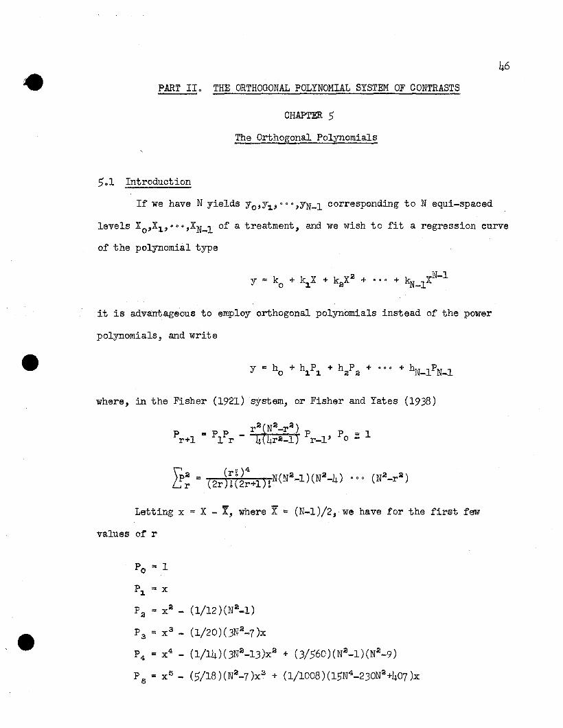
501 Introduction
If we have N yields Yo'Y1,···,YN-l corresponding to N equi-spaced
levels Xo,X1,··0,XN_l of a treatment, and we wish to fit a regression curve
of the polynomial type
y = k + k X + k X2 + o. 0 + k XN- lo 1 2 N-l
it is advantageous to employ orthogonal polynomials instead of the power
polynomials, and write
y = h + h P + h P + 000 + hN lPN' 1o 11 22 - -
where, in the Fisher (1921) 'system, or Fisher and Yates (1938)
Letting x = X - I, where I = (N-l)/2, we have for the first few
values of r
P2 = x2 - (1/12)(N2_l)
P3 = x 3- (1/20)(3N2-7)X
P4 = x4 - (1/14)(3N2-l3)x2 + C3/560)(N2-l)(N2-9)
P5
= x 5 - (5/l8)(N2-7)x3 + (1/1008)(15N4-230N2+407)X

47
Let Pri denote the numerical value of the orthogonal polynomial of
degree r at the level 10 With the object of illustrating confounding
prooedures, write P . = ~ .M ., where M . ::: P. and ~ . will be eitherrl rl rl rl rl rl
- or + or 0 0 Some of these values are presented in Table 4 for the first
four orthogonal polynomials, when N is even and when N is odd. In the
table a oommon factor has been taken out to simplify typographyo Note that
when N is odd, the central element of M when r is odd is unspecified.r
This does not matter in the confounding, since the blocking will proceed
only on the signs. Those elements of ~ . given explicitly in the table,rl
retain their signs independent of the size of N; the others depend on the
size of N"
Table 5 supplies the values of P r. ::: }..P i for N through 8" Fromrl, r
the table it can be ascertained that for N even, the elements of P arer
symmetric about the origin; for N odd, the central element is 0 and the
other elements are symmetric about this central element"
5.2 Partial and Complete Confounding
Let P ::: ~ M denote the diagonalized vector-r -r-T
D(~ M ~ M H. ~ M )ro ro' rl rl' 'r,m-l r,m-l
::: D(~ ~ • •• ~ )D(M M " •• M ).ro' rl' , r,m-l ro' rl' 'r,m-l'
let
p =.~ M = D(~ M ~ M 0 ,," ~ M )-a -s-s so so' sl sl' , s,n-ls,n-l
::: D(~ ,~ l'o •• ,~ . l)D(M ,Ml,···,M 1);so s s,n- so s s,n-
let
!:t = ~t~t ::: D("\oMto'''\lMt 1'''· ·,o<.c,p_lMt,p_l)
"" D("\0'''\1'''· "'''\,p-l )D(MtoilMtl' " "",Mt ,p-l)·

48
Table 4.. Signs and absolute values of the orthogonal polynomials ..
N even
x :x: M3
+ 3 I( 2S_N2 )1
o -(N-l)/2 - (N-l) + 2(N-l)(N-2) + 8(N-l)(N-2)(N-3)(N-4)
Is (N-2) (N-3)(N-4) (N-2l)1
- 2(N-l)(N-2)(N-3)
12(N-2) (N-3)(3-N)1
\3 (JN2-52 )J... 3(N2-4)
- 13(4-N2 )1
3(52-3N2)
\2(N-2) (N-7)1
1(28-N2)\
_ (N2_4)-l..5 3
'-0 .. 5 1
1 -(N-3)!2 - (N-3)
N-l (N-l)j2 + (N-I) + 2(N-l)(N-2) + 2(N-I)(N-2)(N-3) '" 8(N-l) (N-2)(N-3)(N-4)
2 12 40 560
N odd
P1 P2 P3 P4
--X X ~ M1 ..(2 Ma ..(3 M,3 ..(4 M4- -
o -(N-l)/2 - (N-l) ... 2(N-l)(M-2) - 2(N-l)(N-2)(N-3)
1 -(N-3)/2 - (N-3)
... 8(N-l)(N-2)(N-3) (N-4)
-2/2 2 1(13-N2 )1
0 o unsp (N2_l)
2/2 + 2 I(13-N2 )1
N-l (N-l)/2 + (N-l) + 2(N-l)(N-2)
13(N2--9) ,(N2-4l )L-
o unspecified +, 3(N2-1)(N2_9)
6(N2-9) 13(N2-9)(N2 -4l )1
... 2(N-l)(N-2)(N-3) + 8(N-l)(N-2)(N-3) (N-4)
2 12 40 560I I denotes a.bsolute value.

Table 50
N "".3p' pe p'
(') 1 2
+1 -1 +1.+1 0-2+1 +1 +1
11.3
N "" 2
p' p'(') 1
+1 -1+1 +1
1 2
Numerical values of p' ",,}.pr r
N "" 5Pb Pi P~ P; Pl
+1 -2 +2 -1 +1+1 -1 -1 +2 -4+1 0 -2 0 +6+1 +1 -1 -2 -4+1 +2 +2 +1 +1
1 1 1 t*
N "" 4pi pe P' pio 1 2 :3
+1 -3 +1 -1+1 -1 -1 +3+1 +1 -1 -3+1 +3 +1 +11 2 1 10
3
H "" 8pi pi
6 7
N =: 7
P6 Pi Pk P1 Pl P~ P~
+1 -.3 +5 -1 +.3 -1 +1+1 -2 0 +1 -7 +4 -6+1 -1 -3 +1 +1 -5 +15+1 0 -4 0 +6 0 -20+1 +1 -3 -1 +1 +5 +15+1 +2 0 -1 -7 -4 -6+1 +3 +5 +1 +3 +1 +1
17 7, IT1 1 1 'bl225b"O
N =: 6pI pi pi pi p' pi
o 1 2 :3 4 5
+1 -5 +5 -·5 +1 -1+1 -.3 -1 +7 -3 +5+1 -1 -4 +4 +2 -10+1 +1 -4 -4 +2 +10+1 +3 -1 -7 -3 -5+1 +5 +5 +~ +1 +1
3 L 211 2 2' '3 12 10
49
+1 -7 +7 -7 + 7 - 7+1 -5 +1 +5 -1.3 +2.3+1 -.3 -3+7 - .3 -17+1 -1 -5 +3 + 9 -15+1 +1 -5 -.3 ... 9 +15+1 +3 -3 -7 - .3 +17+1 +5 +1 -5 -1.3 -2.3+1 +7 +7 +7 +. 7 + 7
2 ~ 71 2 1 '3 l2 10
+1- 1-5 + 7+9 -21-5 +35-5 -.35+9 +21-5 - 7+1 + 1

Then, as before in the m x n x p factorial experiment, any contrast
between the Yijk can be written
(A B Ct) '" JiP P ptYr 8 r s
"" J'..<. -< ~.M M Mtyr sur 8
when not all three r, 8,tare s:i.mult aneously zero 0
If we wish to confound the contrast ArBsCt the confounding will be
based on whether ..<. ,..<. ,~. is -, or +, or 0, from the following factorr s u
combinations.
A B C
ijk 0 1 2 ... (m-l) 0 1 2 ... (n-l) 0 1 ... (p-l)
rat -< ~l "\.2 ..<. ..<. ..<.81 "<'52 ..<.s,n-l ..<. -<tl -<ro r,m-l so to t,p-l
Any treatment combination ijk· (i "" 0,1,·." ,m-l; j =: 0,1,.·. ,n-l;
k =O,l, ••• ,p-l) ~asblock indicator ..<...<. "<'t."" -, or +, or 0, depending on- rs·
the sizes of m, n, p and the degrees r,s,t. If M "" M =: Mt '" I, contrastr s
(A Be) will be completely confounded with blocks based on the above oon
founding scheme; otherwiseg it will be partially confounded. Note that Pa
for 4 levels and P1 for 3 levels are the only eases within the range of
Table 5 that will allow complete confounding.
5.3 Partitioning of the Polynomial Values
Inspection of Tables 4 and 5 reveals that for even N, the elements
of any even degree polynomials (P ,P , .•• ) will consist of N1, duplicated
negative elements (a total of :ft :0: 2N1. negative elements) and Na dupli
cated positive elements (N+ "" 2Na ); hence 2N1. + 2N2 "" N" These

polynomials will be denoted by Pe when the elements are rearranged so that
the first 2N1 elements are negative and the last 2N2
are positive.. The
vector of these elements is
P~ = (el1,e11,oo .. ,elN1 ,elN1.; 1921, 1921' n .,e2Na,e2Na)
= (P~-; P~)
where eli denotes a negative element and e2i a positive element ..
The odd-degree polynomials (P1'P3
' ..... ) will consist of Q = N/2
negative elements and Q positive elements, the absolute value of each
negative element being matched by a duplicate positive element" These
polynomials will be denoted by Pu if the elements are rearranged so that
the first Q elements are negative and the last Q are positive. The vector
of these elements is
P~ = (-U1,-U2,···,-uQ; u1,ua,···,uQ)
= (P~-; P~+)
Note that for P , it is unnecessary to use a subscript notation to denoteu
whioh elements are negative and which positive. If the observations are
ordered according to either a P or a P , the other even degree polynomials19 u
when ordered conformably will be indicated as PElpe or PElpu ; similarly
the other odd degree polynomials when ordered conformably will be indicated
as pulpe or Pu/pu • E includes e and U includes u, unless otherwise speci
fied. These vectors are indicated in Table 6a"
In Table 6a the element s of PEIP19 and pul P19 have the same subscript
notation as for Pe; similarly PE/PU
and pulpu have the same subscript
notation as P. Each pair of equal elements in any P will correspond tou e
a pair of equal (in absolute value) elements of any Pu; similarly each pair

Table 6a Q Partitioning of the orthogonal pOlynomials.1I52
Pe
••Q
81N1
elN1
~eo
e2a
·""e2Na
e2Na
(1-6)eo
Q
Q
Q
•."E2Na
E2Na
(l-S)Eo
If N = 2Q + 1
-Un
....(>
~a1
-U21
"."U2Na
-U2Na
o
..
(>
Q
"
o
"
Eo
".."
o
Yeli is negative and e2i is positive; ui is positive" Ei and Ui are
negative or positive elements in PE and PU' corresponding to elements
in P and P" If N = 2Q, omit the last line and the e lines. Ife u 0
N = 2Q + 1, a negative e belongs to the 81 group and a positive 8 too 0
the ea group; this is indicated by Be where ~ = 1 if e is negativeo 0
and 8 = 0 if e is positive.o

53
of equal elements of PE will correspond to a pair of equal (in absolute
value) elements of any P. Hence if one partitions P' into the two partsu e
P~_ and P~+, pul Pe will be unconfounded; similarly for PEIpu if P~ is par-
titioned into P~_ and P~+. PElpe and Pu \pu will be confounded under these
conditions. These results are summarized in Table 6b.
Table 6b. Sums of elements of conformable parts.
N = 2Q N = 2Q + 1
B~ock PE1Pe PulPe PEIPu pulpu PEIPeY pulpe PelPE PulPu
1 (-) 2~li 0 0 -Eri 2~li + bEo 0 -E /2 -Eri0
2 (+) -2L~i 0 0 Eri -2~li - SEo0 -E /2 Eri0
3 (0) E 00
Ys = 1, if e is negative; 0 if e is positive.·00
For odd N (N = 2Q + 1), the odd degree polynomials have a zero
element and the even degree polynomials an extra negative or positive ele-
ment; the latter is indicated by eo or Eo. Henoe
pt = (Pl. pI ) ! P' = (pI pI 0)e e-' e+ , u u-' u+'
where either pI or PI+ has Q + 1 elements, depending on whether e is-e- e 0
or +. Hence confounding based on these subvectors will result in unequal
sized blocks. In this case PElpu will be confounded, but Pu fpe will still
remain unconfounded. These results are also summarized in Tables 6a and6b.
504 Bundles of Homogeneous Order
A bundle of homogeneous order was previously defined as that set of
contrasts with properties such that when any single contrast belonging to

54
the set is confounded, all other contrasts belonging to the set will also
be confounded.
The theorems in Chapter 3 could be extended to study the confounding
of (AnBSCT) \(ArBsCt ); however, the results in Table 6b can now be employed
to exaIlline the confounding of (~BSCT)I(ArBsCt ) for different values of
m,n,p and the subscripts. For example, i~ A1 B1C1 is confounded for
m :: n :: p = 4, then (A1 B1 C3), (~B3C1)' (A3~Cl)' (A1BsCa), (AaB1 C3),
(A3BsC1 ), (AaBsCa)1lill be confounded automatically. Hence the homogeneous
bundle of contrasts corresponding to the contrast (Ill) will be (111,113,
131,311,133,313,331,333), indicated as [111].
Oonsidering m x n x p factorial experiments, Table 7 shows the bundles
of contrasts of homogeneous orders obtained in the 4 x 4 x 4 and 4 x 3 x 3
experiments. The second-last column in the table gives the bundles obtained
by the application of the theory of Galois fields, where these exist.
A Galois field can exist only for a prime number or a power of a prime
number. Hnece the six contrasts of the interaction AB in the 4 x 3 x 3
factorial cannot be split into bundles according to Galois theory, since
6 is neither a prime number nor a power of a prime number.

55
Table 70 Allocation of contrasts to homogeneous bundles.
Effect Constituent contrasts of bundles
Number ofcontrastsper bundle
Number ofcontrastsper Galois
bundledf
4 x 4 x 4 factorial experiment
1,2
3,3,3,3, 273,3,3,3,3
A
B
C
IE
AC
Be
ABC
300200 100
030020 010
003002 001
330310
230 320 130220 210 120 110
303301
203 302 103202 201 102 101
033031
023 032 013022 021 012 011
333331313133
233 323 332 311231 321 312 131
223 232 322 213 123 132 113222 221 212 122 211 121 112 111
1,2
1,2
1,2,2,4
1,2,2,4
1,2,2,4
1,2,2,2,4,4,4,8
3
3
3
3,3,3
3
3
3
9
9
9
4 x 3 x 3 factorial experiment
A 300200 100
1,2 3 3
020020 010
2 2
nonexistent 6
nonexistent 6
AB
AC
002002 001
320 310220 210 120 110
302 301202 201 102 101
1,2
1,1,2,2
1,1,2,2
2 2
42,2
nonexistent 12
1,1,1,1
322 321 312 311 1,1,1,2,222 221 212 122 211 121 112 111 1,2,2,2
022022 021 012 011
ABC
17If 020 is confounded, 010 will be unconfounded; if 010 is confounded,020 will also be confounded. Similarly for C and 011 of BC 0
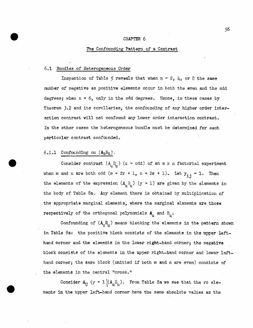
56
CHAPTER 6
The Confounding Pattern of a Contrast
601 Bundles of Heterogeneous Order
Inspection of Table 5 reveals that when n = 2, 4, or 8 the same
number of negative as positive elements occur in both the even and the odd
degrees g when n = 6, only in the odd degreeso Hence, in these cases by
Theorem 30 2 and its corollaries, the confounding of any higher order inter-
action contrast will not confound any lower order interaction contrast.
In the other cases the heterogeneous bundle must be determined for each
particular contrast confounded.
6.1.1 Confounding on (AuBu).
2s + 1)0 Let Yij = 10 Then
= 1) are given by the elements inthe elements of the expression (A B ) (yuu
Consider contrast (A B ) (u = odd) of an m x n factorial experimentuu
when m and n are both odd (m =2r + 1, n =
the body of Table 8ao Any element there is obtained by multiplication of
the appropriate marginal elements, where the marginal elements are those
respectively of the orthogonal polynomials A and B au u
Confounding of (A B ) means blocking the elements in the pattern shownuu
in Table 8a: the positive block consists of the elements in the upper left-
hand corner and the elements in the lower right-hand corner; the negative
block consists of the elements in the upper right-hand corner and lower left-
hand corner9 the zero block (omitted if both m and n are even) consists of
the elements in the central "crosso"
Consider AU (y = 1 \(AUBU
) 0 From Table 8a we see that the rs ele
ments in the upper left-hand corner have the same absolute values as the

57
Table 8a. Blcokin~ 'pattern due to confounding of (AuBu ) when m and nare addb'.
e , t e ze a row~,e1e erIf n is e e ,is removed.
A~ -ubI -ub2... -ubj
...-~s ° ubI ~2
... ubj• 00
ubs
-ual-ua2
• (-,- ) :::: + (-,0) (-,+) :::• -• ==-u . 0a.J..•••
-nar
0 (0,- ) ::: 0 (0,0) (0,+) ::: 0
ual,!
ua2e (+,-) :: (+,0) (+, +) :::: +• -e
==uai 0•e
•uar
11 vn th z a co umn is r moved· if In 's ev·n h r
rs elements in the lower right-hand corner, but will have opposite signs,
and will accordingly cancel in the positive block; similarly for the negative
and zero blocks; hence Aul (AuBu ) will be unconfounded. In a similar manner
~\ (AuBu ) can be shown to be unconfounded. These results are valid for all
values of In and n.
Next consider AE I(AuBu ). For In and n both odd, the sum of the ele
ments in the various sectors of Table 8a are presented in Table 8b, using
the notation of Tables 6a and 6b. Since AE (y ::: 1)I(AuBu ) f 0, this con
trast is confounded with blocks. Similarly BE I(AuBu ) is confounded with
blocks when In and n are both odd. If In is even and n is odd, the row of
the zero block is removed in Table 8b and E == 0; hence ~-I(A B ) is·ao -"E u u

58
unconfounded with blocks; however, BE \(AuBu ) will still be confoundedo
Similarly, if m is odd and n is even, BE I(AuBu ) is unconfounded with blocks,
but L I(A B ) will still be confounded (E r 0), although the column of~ u u ao
the zero block is removed) 0 If both m and n are even, both ~I(AuBu ) and
~ j(AuBu ) are unconfounded with blockso
Table 8bo Sums of elements of ~ (AB ) (y = 1) corresponding to blockingpattern in Table 8ao u u
EalEa2ooo
·oo
Ear
Eao
&
o·oo·Ear
-(sE )/2ao
-sEao
-(sE )/2ao
-(E )/2ao
Eao
-(sE )/2ao
sEao
-(sE )/2ao
Finally let us consider the two-factor interactions. From the work
on homogeneous bundles we know that any odd order contrast (.AuBU) I(AuBu
)
will be confounded for any m and no That is, the contra5ts (00) belong to
[uu], the homogeneous bundle of the contrast (uu)o The amount of confound-
ing is easily determined from Table 6b o

59
(AUBU) (y :: 1) !(AuBU
)+ :: 2(L.uai )(LUbi )
(Au11J) (y :: 1) I(AuBu )_ ::" -2 (LUai)(IUbi )
The same applies to (~~) I(AuBu ) for both m and n odd; however, if either
m or n is even, (~BE)I(AuBu ) is unconfounded with blocks. Finally we find
that (~Bu)I(AuBu ) and (Au~)I(AuBu ) are not confounded with blocks for any
m or n. For example
(~Bu) (y :: 1) \(AuBu )+:: (-Eao/2)(-L..ubi) + (-Eao/2)(L.Ubi ) :: 0
6.1.2 Confounding on (!aBe)
As indicated in Table 6b, the blocking pattern for B will have onlye .
two parts, regardless of whether n is even or odd. If n is even, there are
n_ :: 2n1 negative and n+ :: 2n2 positive elements; if n is odd and the middle
element is negative, n_ :: 2n1, + 1; if n is odd and the middle element is
positive, n+ :: 2n2 + 1. The blocking pattern based on confounding of
(A B ) is presented in Table 9.u e
Using Table 9, we see that
Au (y:: 1)\ (AuBe )+ :: (2n2
Au (y :: 1) \(AuBe )_:: (2n1
Au (y :: 1) \(AuBe)o :: 0
Hence Au I(AuBe ) will be unconfounded with blocks only when n is even
(51 :: 82 :: 0) and n1, :: na ; that is, n_ :: n+; this is true for all mo
From Table 6b we see that BU (y :: 1) \Be :: 0 for all sectors; hence
Bul(AuBe ) is unconfounded with blocks for all m and n. The sum of the
elements of BE (y :: 1) \(AuBe ) has the same absolute value but opposite
signs for the two parts of each block. Hence BE I(AuBe ) is unconfounded
with blocks for all m and no AU I(AuBe ) will be unconfounded with blocks

60
Table 90 Blocldnv·attern due to the confounding of (A B ) and contrast1 u etotals.
(y = 1) = -(2n.a + ba)E /2ao
BE (y = 1) = -r(2L.~1.i+5J.~o)
~- (y = 1) = -(2na + ba»)U .-lJ L;, aJ.
~
Au (y = 1) = -(2nJ. + oJ. )L.Uai
~ (y = 1) = -(2n1 + bJ.)Eao/2
BE (y = 1) = r(2L.~1.i+SJ.~o)·•
-uai
-uar
o
~: set r = 1 above
Au = OJ ~ = (2na+Oa )Eao
BE: set r = 1 above
u Au (y = 1) = (2n1 +~1 )LUai Au (y = 1) = (2na+'8a )LUaial•·· (y 1) AE
(y 1)u ~ = =ai as in (- -) sector in (- +) sector; as
uar BE (y = 1) BE (y = 1)
lIOmit the zero row if m = 2r If n = 2s, abo does not exist; hence, set
~J. = 8a = O. If n = 2s +1 and ebo is -, 81 = land Sa = 0; if ebo is +,
~1 = 0 and O2 = 1 0
only if m is even (so that E does not exist) for all values of nj if mao
is odd, ~\(AuBe) will be confounded with blocks for all values of n.
Since Eo (y = l)\Be = 0 for all sectors in Table 6b, (AEBu)I(AuBe )
and (AuEo) \(AuBe ) are unconfounded for all m and n. As for (~BE)' we
note that
(~~) (y = 1) \ (AuBe )+ =(L~li+OI\O)(-·(Eao/2)+(Eao/~))= 0
and similarly for the other blocks. Hence (!EBE)\(AuBe) is also unconfounded
with blocks for all m and no Finally we note that

61
(~~) (y = 1)\ (AuBe )+ = -2(2L~lj+(\Ebo)LUai
(~BE) (y = 1) I(AuBe )_ = 2(2L\lj +01\o)L:.Uai
(AuBE) (y = 1) \(AuBe)o = 0"
Hence (~BE)I(AuBe) is confounded with blocks for all m and n; i"e", (UE)
belongs to rue].
The blocking pattern here can be set up as in Table 9 by using
ebl and eb2 for Be and eal and ea2 for Ae; this is done in Table 10"
Table 10" Blocking pattern due to the confounding of (A B ) and contrasttotals •.!! e e
If m 2r, eao does not ex~st (Oal 0a2 0), s~~larly for ObI and bb2
if n = 28. If m = (2r+l) and e is -, 0 1 = 1 and B 2 = 0; if e is +,ao a a aoSal:: ° and ba2 = 1; similarly for bbl and 0b2 if n = (2s+l).
BA e
eb1n1 sb1n1 bbleboebll ebll... eb2l eb2l
... e e ~ ee b2na b2na 2 bo
ealleall ~(y=l) = (2n], +Obl ) (2~ali ~(Y=l) = (2n2 +Sb2 )( 2LEali""
+ b IE )" + b IE )eam1 a ao a ao
e BE(y=l) = (2~+bal )(2L~lj BE(y=l) =-(2m1 +bal ) (2lEbljam],o e
+ bbl\O) + °bll\o)al ao
ea2l ~(y=l) = -(2n], +obl)(2IEali ~(y::l) :: -(2n2+~b2)(2LEaliea2l + 0 IE + 8 E· a ao al ao·· (2m2 +8a2) (2Ll\lj :: -(2m2+8a2)(2L~lje BE(y=l) = ~(y::l)a2m2e
+ °blEbo) + 8bl~O)a2m2o ea2 ao
y.:: = :: • .

62
From Table 10 we see that
This expression equals zero only whenn is even (6b1 = bb2 = 0) and n1 = na,
so that n_ = n+, but m can be any value. Similarly
hence 11: \(AeBe ) is unconfounded with blocks only when m is even and m1 = ma
(so that m_ = m... ), but n can be any value. As in system 6.1.2, Au \(AeBe )
and 11T\(AeBe ) are unconfounded with blocks for all m and n.
As for interactions, those involving Au or 11T will be unconfounded;
however, (AEBE)\(AeBe ) will be confounded with blocks for all m and n:
Hence (EE) belongs to fee].
6.104 Summary
Table 11 summarizes all the findings on polynomial confounding of
main effects and two-factor interactions when specific two-factor inter-
actions are confounded. The results in Table 11 can be verified by app1y-
ing the conditions of Theorem 3.3, Corollary 3.3.1, and Table 6b. Consider,
for instance, the value of Au (y = 1) I(AuBe ), when mis odd andn is even;
since tr ~3 = 0, AuI(AuBe ) will be unconfounded when n+ = n_.

63
Table 110 Confounding of general contrasts when specific AB contrasts areconfounded.Y
Specific confounded effect
K denotes confoundingo *' lndlcates an lmposslble set of m and n, for
example m must equal mfor a.ll odd contrasts, A 0 All main effects- + u
and two-factor interactions omitted from this table are not confounded
for any m or no
,,
(A B. ) (A B ) (A B ) ! (A B )Value of uu u e e u e e
m andn ~ BE (AuBU) (AEBE) ~ AE (AuBE) Bu BE (AEBu)i AE BE (AEBE)I!
Both odd K K K K ,K K K IK K K K K K
m odd n =n K 0 K 0 0 K K K 0 K 0 K K- . +
n even n:,.fn+ *' *' *' *' K K K *' * * IK K K
Im even m =m 0 K K 0 K 0 K 0 K K ! K 0 K
- + ,odd m_fm+ *' *' * *' *' *' *' K K K i K K Kn
m =m- + 0 0 K 0 0 0 K 0 0 K 0 0 Kn =n- +
m =m- +
*' *' * *' K 0 K * * *' Kn_fn+K 0
m even -n even m_fro",
*' * * *' *' *' *' K 0 K 0 K Kn =n
- +
m.Jm+*' *' ;Eo *' *' * *' *' *' *'n fn K K K
- +
11 . . .
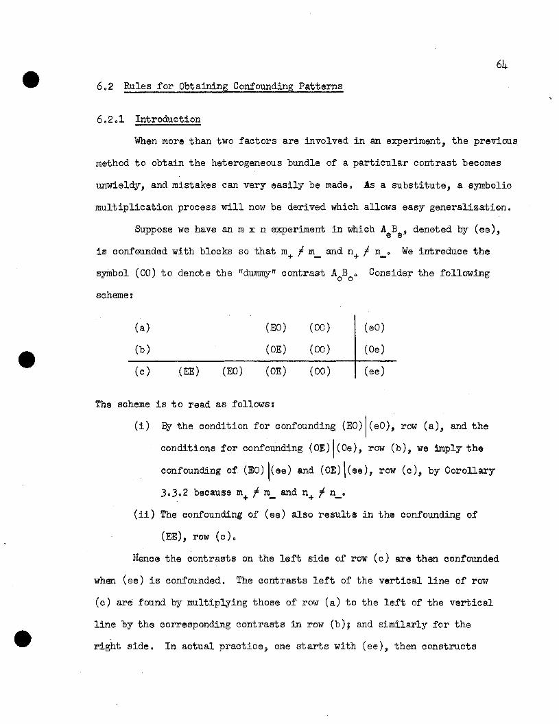
64
6.2 Rules for Obtaining Confounding Patterns
6.201 Introduction
When more than two factors are involved in an experiment, the previous
method to obtain the heterogeneous bundle of a particular contrast becomes
unwieldy, and mistakes can very easily be made. As a sUbstitute, a symbolic
multiplication process will now be derived which allows easy generalization.
Suppose we have an m x n experiment in which A B , denoted by (ee),e e
is confounded with blocks so that m+ f m_ and n+ f n_. We introduce the
syinbol (00) to denote the "dU1lJIllyll cont-rast AoBoo Consider the following
scheme:
(a) (EO) (00) (eO)
(b) (OE) (00) (De)
(c) (EE) (EO) (OE) (00) (ee)
The scheme is to read as follows:
(i) ~ the condition for confounding (EO)\(eO), row (a), and the
conditions for confounding (OE) I(Oe), row (b), we imply the
confounding of (EO) Ieee) and (OE) Ieee), row (c), by Corollary
30302 because m+ f m_ and n+ f n_o
(ii) The confounding of (ee) also results in the confounding of
(EE), row (c)o
Hence the contrasts on the left side of row (c) are then confounded
when (ee) is confounded. The contrasts left of the vertical line of row
(c) are found by multiplying those of row (a) to the left of the vertical
line by the corresponding contrasts in row (b); and similarly for the
right side. In actual practice, one starts with (ee), then constructs

65
(Oe) and (eO), then the left side of (a) and (b) and finally the left side
The introduction of the dummy contrast is an all-important step,
since this fictitious contrast allows us to obtain the heterogeneous
bundle of a higher order interaction contrast from the homogeneous bundles
of those lower order interaction contrasts, whose symbolic product is equal
to the higher order interaction contrast o
The above scheme gives the heterogeneous bundle of the contrast (ee)
only when mo+- t m_ and no+- t n_o Generalization to other values of m and n.
and other polynomial contrasts is required o It will be shown that by using
the properties of othogonal polynomial contrasts and by adopting appropri-
ate conventions with respect to the dummy contrast, the heterogeneous
bundle of any higher order interaction orthogonal polynomial contrast can
be obtained from the symbolic multiplication schemeo This is accomplished
by the provisions of Corollary 30302 when constituting the heterogeneous
bundle 0
6.202 Polynomial confounding patterns for anm x n experiment
One would prefer to substitute the bundle notation for the contrast
notation in Section 60201 and thus generalize these results to both odd
and even contrasts 0 If all confounding contrasts were of even degree,
[eO] = (EO) for all m; hence the use of the bundle notation would be satis
factoryo However, [uO] = (UO) for even m and [uO] = (UO) + (EO) for odd m;
a general bundle notation becomes unsatisfactory 0 In Table 12 we extend
the scheme of Section 60201 to each type of polynomial confounding pattern,
for any m and no In order to fulfill the provisions of Corollary 303 0 2,
(00) is used or omitted in different situations o Also one will have
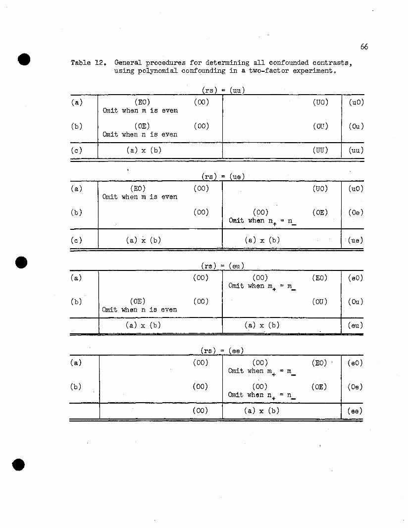
Table 120 General procedures for determining all confounded contrasts,using polynomial confounding in a two-factor experiment.
(rs) = (uu)
66
(a) (EO) (00) (UO) (uO)Omit when m is even
(b) (OE) (00) (OU) (Ou)Omit when n is even
(c) (a) x (b) (UU) (uu)
(rs) = (ue)
(a) (EO) (00) (UO) (uO)Omit when m is even
(b) (00) (00) (OE) (Oe)Omit when n+ ::: n_
(c) (a) x (b) (a) x (b) (ue)
(rs) ::: (eu)
(a) (00) (00) (EO) (eO)Omit when m+ = m_
(b) (OE) (00) (au) (Ou)Omit when n is even
(a) x (b) (a) x (b) (eu)
(rs) = (ee)
(a) (00) (00) (EO) (eO)Omit when m+ = m_
(b) (00) (00) (OE) (Oe)Omit when n+ ::: n_
(00) (a) x (b) (ee)

67
separate. sections for (E) and (U) contrasts; the use of these will be
dictated by the absence or presence of each in the homogeneous bundles of
the confounding contrasts. The :multiplicative schemes are simply conveni-
ent arithmetical devices to produce the results of Table II. A separate
Bcheme is constructed for each of the four general two-factor confounding
contrasts (ra) = (uu), (ue), (eu) and (ee).
6.2.3 A general rule for obtaining the confoundingpatterns of any polynomial contrast in anm x n factorial experiment
In previous chapters (RS) has referred to any two-factor contrast
with (ra) being a given confounding contrast. If we now use the restricted
Rf to refer to only odd degree contrasts if r is odd and to even degree
contrasts if r is even, and similarly for S· and s, we can generalize the
four parts of Table 12 into a sin~le part, as in Table 13.
Table l3.Y Generalization of the parts of Table 12 ..
(a)
(b)
(EO)Omit when r = eOmit when m is even
(OE)Omit when 13 .. eOmit when n is even
(00)
(00)
(00)Omit when r = uOmit when m..... m_
(00)Omit when 13 .. uOmit when n..... n_
(rO)
(as)
(c) (a) x (b)
Y(R-O) .. {(UO) if r .. U and. (EO) if r .. e
(a) x (b)
(OS') I: i(OU) if 13 .. u and. I(OE) if s .. e
(rs)
6.2.4 Confounding pattern of .any polynomial contrastin an m x n x p factorial experiment
Since all the theorems that affect the confounding pattern of any
particular contrast of an m x n experiment are embodied in this rule, ex-
tension of the rule to an m x n x p or larger experiment will be valid.

68
Such extension is straightf'orward and given below to obtain the confounding
pattern of any contrast (rst) of an m x n x p experiment.
Table 14. Confounding pattern for any polynomial contrast in an m x n x pfactorial experiment.!!
(a) [eOO] (000) (000) (R100) (rOO)Omit when r is even Omit when r is oddOmit when m is even Omit when m.., = m_
(b) [OeO] (000) (000) (OS"'O) (OsO)Omit when s is even Omit when s is oddOmit when n is even Omit when n. = n_
(c) (OOe] (000) (000) (OOT"'') (Oot)Omit when t is even Omit when t is oddOmit when p is even Omit when p. = p_
(d) (a) x (b) (a) x (b) (rsO)
(e) (d) x (c) (d) x (c) (rst)
Y See footnote to Table 13. T~ is treated as R~ and S~ in that table.
In practice is is simpler to first obtain row (d) and then row (e).
6.2.4 Polynomial confounding patterns for anm x n x p experiment
Table 15 supplies the confounding patterns of the f'our basic con
trasts of highest order of an m x n x p experiment: (uuu), (uue), (uee),
(eee). Any other contrast can be found by permuting factor letters; i.e.,
(ueu) is obtained by interchanging B and C in (uue). As before, K denotes
the contrast belonging to the heterogeneous bundle of' the confounding con-
trast.

Table 15. Confcunding patterns of the four basic contrasts of highestorder of.an m x n x p experiment.
69
(uuu) (eee)
mjm_ m.jm_ mjm_ m =In+ -
All odd All n.jn_ njn_ n =n n cnp even n,p even even + - + -
pjp- P =p P =p P =p+ - + - + -
(EOO) K K K K(OEO) K K K(OOE) K K K
(EEO) K K K(EOE) K K K(OEE) K K K K(EEE) K K K K K(UUU) K K K K
(uee)
m odd m evenn)n_ njn_ n =n nJn_ n)n_ n =n
+ - + -pjp- P =p P =p pjp- P =p P =p
+ - + - + - + -
(EOO) K K K(UOO) K K
(UEO) K K(UOE) K K K K(UEE) K K K K K K
(uue)
m,n odd In odd, n even m,n even
PjP- p =p pip_ P+=P- pjp- p =p+ - + -
(EOO) K K K K(OEO) K
(EEO) K K(000) K K K(UUE) K K K K ·K K

70
6.3 Determination of the Coefficients of theBlock Constants
Whenever a contrast is confounded with blocks, its expectation will
contain some linear combination of the block constants. The coefficients
of this linear combination may be obtained by application of the Bainbridge
technique (Binet et aI, 1955), or by any easy extension of the rule used to
derive the heterogeneous bundle of the contrast confounded.
Consider first contrast (A B Ct ) of the m x n x p experiment.r s .
When a , b , ct are partitioned into negative and positive parts, ther s
expression J' arbsct J can be written as
J1a b c J ~ (tr!r_)(tr E.sJ(tr 2.t ... ) ... (tr !r_)(trE.s... )(tr '£t-)
• (tr !r.)(tr E.sJ(tr 2.t-) (tr !r+)(tr E.s+)(tr .sc.,)+ (tr !r_)(tr E.s_)(tr '£t-) (tr!r_)(tr E.s+) (tr '£t ... )
... (tr !r... )(tr E.s_)(tr '£t ... ) + (tr !r+)(tr E.s ...)(tr .£tJ
= (ArBsCt )+ + (ArBsCt )_
The values (ArBsCt )+ and (ArBsCt )_ will respectively be the coefficients
of the block constants in the expectation of the confounded contrast
(A B Ct. ).r s
In any particular case, when the traces of the parts of the vectors
are lmown, the block coefficients may be obtained by inspection of the
expression
Consider, for example; the confounding of the contrast (A4B2C1 )
of the 5 x 3 x 2 experiment.

71
Since
!4 ~ D(+1,-4,+6,-4,+1),
~2 .. D(+1,-2,+1),
S ~ D(-l,+l)
tr a .. -8 tr b = -2 tr c = -1-4- -2- -1-tr 2:4+ = +8 tr b2+ ~ +2 tr £1+ = +1~
Consider the expression (+8,-8)(+2,-2)(+1,-1); the coefficient of the posi-
tive block becomes
(8 x 2 x 1) ... (8 x -2 x -1) + (-8 x 2 x -1) ... (-8 x -2 x 1) = 64;
that of the negative block, -64. From Table 15 the heterogeneous bundle
of contrast (421) ·is (421,221,021,401,201,001) ~ The contrast (221) in
this bundle is the contrast (221)\(421) which, since the b and ccoeffici
ents are the same in (221) and (421), may be written (214)(2)(1)~ Since
2:2 = D(+2, -1 ,-2, -1, +2 ), it follows that tr c'!:21I2:4) = -2 and
tr (2:22\2:4) .. +2~ To obtain the coefficients of the block constants in
the expectation of the contrast (221), we have to examine the expression
(+2,-2)(+2,-2)(+1,-1)~ Comparing this expression with that obtained for
contrast (421), it follows that the ooefficients will become 64/4 = 16, and. . a .
-64/4 ::: -16. For the contrast (021) we examine the expression
(+2,-2)(+1,-1), and find the coefficients of the block constants to be
4 and -4. Similar procedures are applied for the contrasts (401),(201),
(001) ~
This work can be systematized as follows:

In 5 x 3 x 2 experiment,
!4 = D(+1,-4,+6,-4,+1)
!2 = D(+2,-1,-2,-1,+2)
.£2 = D(+1,-2,+1)
72
Confounded contrast: (421)
Heterog. bundle
(421) I(421)(221 )I (421)(021) I(421)(401) 1(421)(201 ) t (421 )(001) 1(421)
Partitioned vectors
(+8,-8)(+2,-2)(+1,-1)(+2,-2)(+2,-2)(+1,-1)(+2, -2 ) ( +1, -1 )(+8,-8)( +1.-1)(+2,-2) (+1,-1)(+1,-1)
Block coefficients
(64,-64)(16,-16)( 4,-4 )(16,-16)( 4,-4 )(+1,-1 )

CHAPTER 7
The Confounding Pattern of Twd Contrasts
73
701 Simultaneous Partitioning of TwoOrthogonal Polynomials
We now investigate further partitioning of the polynomial elements
as given in Table 6a. First we will consider the results for even N. As
before, Pe denotes an even polynomial with 2N1 negative elements followed
by 2N2 positive elements (2N1 + 2N2 := N). Let Pellpe denote another even
polynomial with its elements arranged so that the first 2N11 elements are
negative, the next 2N12 are positive, the neri 2N21 are negative and the
final 2N22
are positive (N11 + N12 =NJ.and N21 + N22 = Na). Finally,
let pu\(Pe,Pel ) = pulpel\Pe be any odd polynomial with elements corres
ponding to those of Pellpe. Each pair of equal elements in Pellpe will
correspond to a pair of equal (in absolute value) elements of any PUJ
ioe., there will be a +U and -U for each pair of elements in Pellpe.
Hence Pu \(Pe'Pel) will not be confounded with block effects.
If N is odd there will be a central element OfPel\PeJ this
central value will be either negativa or positive • However, the corres
ponding central value of pu\(Pe'Pel ) = pulpellpe will be zeroo Hence,
whatever the value of N, Pu I(Pe'Pel) will be unconfounded with blocks.
It can readily be verified that this is the only partitioning, in terms
of the simultaneous partitioning of two orthogonal polynomials, that will
yield parts whose elements sum to zero.
Let us now consider the general case of an m x n experiment with
contrasts (ArBs) and (AfBg ) confounded simultaneously (in 4, 6, or 9
blocks). Using the notation of previous chapters,
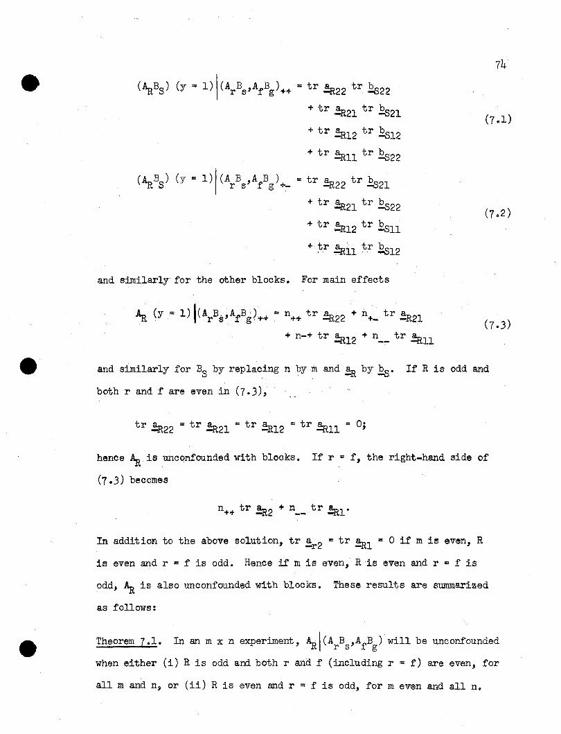
74
(~BS) (y = 1) \ (ArBs,AfBg )++ :: tr ~22 tr 12.s22
+ tr !R2l tr E.s2l
+ tr ~12 tr E.s12
+ tr ~ll tr £S22
(~BS) (y :: 1)1 (ArBs,AfBg )+:- "" tr !R22 tr £S2l
... tr !R2l tr £S22
+ tr !R12 tr £Sll
... :tr .!all :tr E.s12
and similarly for the other blocks. For main effects
Aa. (y = 1) '(ArB$,AfBg~++ :: n++ tr ~22 ... n+_ tr !R2l
+ n-+ tr !:.R12 + n__ tr ~ll
(7.3)
and similarly for BS by replacing n by m and ~ by £S. If R is odd and
both rand f are even in (7.)),
tr~22 "" tr !fl.2l :: tr ~12 = tr ~ll "" OJ
hence Aa is unconfounded with blocks. If r :: f, the right-hand side of
(7.3) becomes
In addition to the above solution, tr ~r2 =tr !fl.l = 0 if m is even, R
is even and l' = f is odd. Hence if m is even, R is even and r "" f is
odd, A.a is also unconfounded with blocks. These results are summarized
as follows:
Theorem 7.1. In an m x n experiment, .t\I(ArBs,AfBg ) will be unconfounded
when either (i) R is odd and both rand f (including l' ::: f) are even, for
all m and n, or (ii) R is even and r = f is odd, for m even and all n.

Afurther examination of (7.1) and (703) indicates the following
Theorem 702. In an m x n experiment, when contrasts (A B ) and (A,&'B ) arers .L.g
confounded simultaneously, contrast (~BS) will be unconfounded when either
~ \ (ArBs,AfBg ) or BSI(ArBs,AfBg ) is unconfounded; ~I(ArBs,AfBg ) will be
unconfounded if ~I(Ar,Af ) is unconfounded and similarly for BS.,
If .Aa is unconfounded, tr ~22 = tr ~21 = tr ~12 = tr !all = 0;
similarly if BS is unconfounded. We have been unable to prove that the
conditions in these theorems guarantee that all other situations produce
.confounded effects; experiments fulfilling theconditions in these theorems
result in unconfounded effects, but other situations may also prevail in
which effects could be unconfounded.
7.2 The Generalized Interaction
'When two contrasts (A B ) and (A,&'Bg ) of an m x n experiment are con-o r s .L
founded simultaneously, then, as shown in Chapter 4, their generalized
interaction (A B ) will be confounded automatically. The usual notationvw
for the generalized interaction of two contrasts is
It is important to observe that this is a symbolic relation only, not an
algebraic one; algebraically, however, av =a at and b =b b 0 Ther w s g
notation is meant to imply that when a new contrast is formed out of the
coefficient matrices of two given contrasts, this new contrast will be
confounded, whenever the two given contrasts are confounded simultaneously.
Assume the matrices a and b are expressible as linear combinations ofv w
other matrices, say

a = araf = ar +f + 0(2ar+f_2 + = L(ar +f ), sayv
b = b b = b + ~2ba+g_2 .... ... = L(bs +g ), sayw s g s+g
where 0(2 and ~2 are constants. In this case,
avbw = L(ar+f)L(bs +g)
= ar+fbs+g + ~2ar+fbs+.g_2 +. o(aar+f_2bs+g + •••
... L(a +fb + )r s g
and
(AvBw) = (Ar+fBs+g) + ~2(Ar+fBs+g_2) + o(a(Ar+f_2Bs+g) + •••
= L(Ar+gBs +g )
Hence, when the generalized interaction of the two contrasts (A B ) andr s
(AfBg ) is expressible in the form of sfinear combination of contrasts,
this linear combination will be confounded when the two contrasts are
confounded simultaneously. It does not follow, however, that each con-
trast in the linear combination will be confounded (see Corollary 4.3.1).
7.3 Reduction Formulae for Products ofOrthogonal Polynomials
The recursion formula of the orthogonal polynomials in the Fisher
system can be written as
It might appear that we would require generalization of this formula to
the case Ps x Pr for the purpose of expressing the generalized inter
action as a linear combination of contrasts, but this is not necessarily
76
so. Consider the product P x P when there are N observations, ands r

77
suppose that s = r = (N-l). Then P x P will equal some linear combinas r
tion of polynomials such as P2(N-l) + ..<P2(N_2) + •••• Since there are only
N observations, all polynomials with degrees higher than (N-l) will vanish,
and the number of terms in the linear combination is greatly reduced.
The number of levels of anyone factor being usually small in
practice, the direct calculation of the reduction formulae, for those cases
likely to be useful, seems indicated. Table 16 accordingly supplies the
reduction formulae of the products for N through 5:
Table 16. Products of polynomials.
N == 3 N == 4 N = 5
P1 X P1. = Pa + 2Po
P1 X Pa == P3 + ~P1
_ 36P1. x P 3 - P4 + 35Pa
P1. x P4 == ~P3
P", X Pa == P + ~ +]#p'" 4 7 a :J 0
P P • 2~ + 36pa x 3 -S.r 3 . 25 :L
10 14lLPa x P4 == '"'TP4 ,+ ~a
P3 x P3 == --ftPa + /:oPo P3 X P3 == -~P4 -172?2 + f~~o
P 3 X P4 == -~P3 + i~~1.
P4
X P4
== 108p _ 288p + 288p245 4 343 a 175 0
P1. X P1 == Pa + tPo
P1. X Pa ;'; P3 +~P1
P1 X P3 == loPa
-1 2P x P == --P + -P Pa x Pa == Poa .2 '3 2 -9 0
Since in practice we use P' == AP, the relations in Table 16 should
be adjusted accordingly before application to a specific problem. In this
chapter we use Table 16 in a symbolical sense only.

78
7.4 The Status of the Contracts in the1inear Combination
1et u and u1
denote odd and e and e1 even confounding contrasts;
ua and ea odd and even contrasts in the generalized interaction. There are
four types of confounding contrasts, depending on the odd-even character
of (rs) and (fg). If r and f are both odd or both even, we call them
similar contrasts; if one is odd and the other even, they are dissimilar
,contra.sts; likewise for sand g. The four types are
Charaoter of contrasts
~ r and f s and g Example
I Similar Similar (ue) x (U1
81
)
II Similar Dissimilar (ue) x (u1 u1 )
III Dissimilar Similar (ue) x (e1 e1 )
IV Dissimilar Dissimilar (ue) x (e1u1 )
Based on the results in Table 16, the form of the generalized
interaction 1((r+f)(s+g)] is given in Table 17, for each of these types.
Table 17. Form of generalized interaction contrast, L[(r+f)(s+g)]Y
Type r r fs t g
r = fs t g
r f fs = g
r = fs = g
I 1(e2e2 ) L{eaea,Oea)
II L(eaua) L(eaua,Oua )
III 1(ua6:a) ~
liT L(uaua) ~
17~ indicates this combination cannot exist ..
For example, in a 5 x 4 experiment: (12) x (31) = L(43), where
(12) = (ue), (31) = (u1u1 ); hence, from Table 16

79
This is a Type II contrast with r r f and s f gj hence L(43) is a sum of
even-odd contrasts. Each individual contrast in L(43) [(43), (41), (23)
and (21)] is confounded. However, it should be emphasized that when the
contrasts (RS), (RO), (OS) belong to the linear combination L[(r+f)(s+g)],
the automatic confounding of this linear combination will not necessarily
confound the contrasts (RS), (RO), (OS). For example, consider the con-
founding of contrasts {32) and (33) of a 4 x 4 experiment. Here
Note that the complete compounding of the subscripts does not hold in
this case, since the sum of the corresponding degrees for each factor
cannot exceed the number 3 = 4 - 1, where 4 is the number of levels.
By Theorem 7.2, (23) 1(32,33) and (21)\(32,33) will be uncOnfoundedj
however, (03) \(32,33) and (01)\ (32,33) will be confounded.
7.5 Confounding Pattern of Two ContrastsConfounded Simultaneously
Consider the simultaneous confounding of contrasts (A B ) andr s
(AfBg) of an m x n experiment. By Corollary 4.1.1, all contrasts belong-
ing to the heterogeneous bundle of (ArBs) [if (ArBs) has a heterogeneous
bundle], and all contrasts belonging to the heterogeneous bundle of
(AfBg ) [if (AfBg ) has a heterogeneous bundle] will be confounded when
(ArBs) and (AfBg ) are confounded simultaneously. Hence the first step
to obtain the confounding pattern of (ArBs,AfBg ) will consist in applying
the rule developed in Chapter 6 to each of the two contrasts separately
(alternatively, Table 15 can be used).

80
Let us now denote the generalized interaction (rs) x (fg) by L(rts'),
where L(rts t ) is a linear combination of the contrasts
(rts t ), (r t (s'-2)), «r'-2)s'), «r'-2)(st-2))···
The expression (RtSt) will refer to anyone of the contrasts in L(rts t ).
According to Table 17, when both r f f, s i g, contrasts of the type
(RtO) and (OS') will not appear in L(rts t ); when r = f and s i g, con
trasts of the type (RtO) will not appear; when r If and s = g, contrasts
of the type (OSt) will not appear. Let [rtst] denote the homogeneous
bundle of the particular contrast (r'st), which can be found in Table 13.
If r t = e' and st = u t , for example, [rts t ] will be the homogeneous bundle
[etu t) = (EU). It follows by the results of the partitioning of the
orthogonal polynomials that if contrast (e tu') is confounded, all contrasts
belonging to the homogeneous bundle [e tu t] will be confounded. Similarly
let [r'O] denote the homogeneous bundle of (rtO) and [Os'] the homogeneous
bundle of (Os').
When both r I f and s f g, L(rts t ) will be a linear combination of
the contrasts belonging to the homogeneous bundle [rtst]; when r = f and
s f g, L(r'st) will be a linear combination of the contrasts belonging to
the homogeneous bundles (rts t ] and (Ost]; when r f f and s = g, L(r'st)
will be a linear combination of the contrasts belonging to the homogeneous
bundles [rts t ] and [rtO]. For example, in a 5 x 4 experiment:
(12) x (31) = L(43), where L(43) is a linear combination of the contrasts
belonging to the homogeneous bundle [43], !!!., (43,41,23,21); in a
4 x 4 experiment: (32) x (33) = L(23), where L(23) is a linear combination
of the contrasts belonging to the homogeneous bundle [23], viz., (23,21)
and to the homogeneous bundle [03], viz., (03,01).

81
By Theorem 7.2, contrast (r's') will be unconfounded by (rs,fg)
when either r'l (r,f) or s'l(s,g) is unconfounded; (r'O) will be uncon
founded if r' \(r,f) is unconfounded and (Os') Vlill be unconfounded if
s'\(s,g) is unconfounded. Hence, under the same conditions, [r's'], [r'O]
and [Os') will also be unconfounded by (rs,fg).
In terms of the theoretical development above, the following stages
can be distinguished in the procedure for obtaining the confounding pattern
of (rs,fg) in an m x n experiment:
(i) Obtain the confounding pattern of the contrast (rs).
(ii) Obtain the confounding pattern of the contrast (fg).
(iii) Determine the linear combination L(r's') = (rs) x (fg) from
Table 16.
(iv) Obtain the homogeneous bundle [r's'] of the contrast (r's')
when r f f,s ; g; the homogeneous bundle [O's) of the con
trast COs') when r = f,s r g; the homogeneous bundle [r'O]
of the contrast (r'O) when r f f,s = g.
(v) Determine the confounding status of the homogeneous bundle
[r's') when r r f,s r g: of the homogeneous bundle [Os']
when r = fjs r g; of the homogeneous bundle [r'O] when
r rf,s = g.
In actual practice, stages (iii), (iv) and (v) can be combined into the
SYmbolic multiplication scheme given below, which embodies the consequences
of the theorems stated above 0
The part to the right of the double vertical line is first written
down; then, [r'O] in row (a) and [Os'] in row (b) are obtained from the
symbolic products (f x r) and g x,s) respectively in Table 16, and the
confounding according to Theorems 7.1 and 7.2, remembering that r' is

82
even if r and f are both even or both odd. Depending on the conditions
given in the scheme, multiply the elements in row (a) by the elements in
row (b) to obtain the elements in row (c), subject to the restrictions that
mu~tiplication across vertical lines is not permitted.
Table 18. Rule for obtaining homogeneous bundles in the generalizedinteraction of the contrasts (rs,fg) of an m x n experiment.
(a)
(b)
(c)
(00)Omit when r 1= f
(00)Omit when s 1= g
[r'O]Omit when r = f isodd for m even
[Os']Omit when s = g isodd for n even
(a) x (b)
(fO)
( Og)
(fg)
(rO)
(Os)
(rs)
When the confounding patterns of contrasts (rs) and (fg) are un-
known, the last two columns of Table 18 can be enlarged to accommodate the
scheme of Table 13.
As an example, consider the confounding of the contrasts (12) and
(31) of a 5 x 4 experiment. Since r f f,s 1= g, (12) x (31):L(43). The
scheme for the generalized interaction becomes
[40]
[03]
[43]
(0)
(01)
(1)
(10)
(02)
(12)
The homogeneous bundle of contrast (43) is (43,41,23,21). From Table 13
the heterogeneous pundles of contrasts (31) and (12) are respectively
01,33,11,13,20,40) and (12,32,20,40). Hence the confounding pattern of
contrasts (31) and (12) is
(33,31,13,11,40,20,43,41,32,12,23,21).

83
Generalization of the rule to experiments with more than two factors is
immediate, as was done in Table 14.
The result s in this chapter presume that the only contrasts which
are confounded when (ArBsCt ) and (AfBgCh ) are simultaneously confounded
are: (i) those contrasts confounded by either (ArBsCt ) or (AfBgCh ),
(ii) possibly some or all of the contrasts in the linear combination of
the generalized interaction (A B C ). We have been unable to prove thatvwz
no other contrasts orthogonal to the confounding contrasts can be confounded;
however, we believe that this is the case, and recommend the above pro-
cedures be used in determining which contrasts are confounded.

84
CHAPTER 8
Confounded Experiments with Equal-sized Blocks
8.1 Confounding a Single Highest OrderInteraotion Contrast
Consider the confounding of contrast (ArBsCt ) of an m x n x p ex
periment. As before, let m_, m+" mo denote the frequencies of the negative,
positive and zero elements respectively of the vector a ; n ,n ,no those-r - +
of the vector .£s; P_'P+'Po those of the vector .£t,. Schematically we have
Blockindicator
+
o
Total
Frequenciesa b 2t-r -s
m n p--m+ n+ P+
mo no Po
m n p
Confounding (ArBsCt ) consists of placing the treatment combina
tions corresponding to a - sign in one block, those corresponding to a
+ sign in another block. Confounding a single contrast, therefore, im-
plies the arrangement of the treatment combinations into 3 or 2 blocks,
depending on whether the 0 block indicator is present or absent.
Let N_, N+, No denote the number of treatment combinations in the
negative block, the positive block, and the zero block respeqtively.
Then, from the above scheme

85
N = m n n + m nn + m n p + m n n_ _ ',.."F_ _.p- + + _ _ + ¥-_
N = mnp - (m-m )(n-n )(p-p )o 000
= mnp - (m+ + m_)(n+ + n_)(p+ + p_)
If No = 0, we need only have N+ = N_ to have equal-sized blocks (there
will be only two blocks in this case). The condition for N+ = N is
(m - m )(n - n )(p - p ) =0+ - + - + -
(8.1)
(8.1) is satisfied if and only if one or more of these conditions hold:
(802)
If N > 0, (8.1) must still be met; however, a second condition is alsoo
imposed:
N+ + N - 2N = 0; or,- 0
3(m-m )(n-n ) (p-p ) = 2mnp000
(8.3)
It is not possible to derive a simple condition, such as (8.2), which will
satisfy (803). One must determine suitable combinations of (m,n,p) for
given (m ,n ,p ) or vice versa. For example, if m = n = 0 and00000
p > 0, P = 3p , and m and n can be any value. In general, if only twoo 0
of the three main effect contrasts have no zero elements, the number of
levels of the other factor must be three times the number of zero elements;
in a.ddition, at least one of the three contrasts must have the same number
of positive as negative elements to satisfy (802)0
Similarly, if m = 0 and n = 1,o 0
3(p-po)n = p _ 3p0 and p =
3(n-l)po ;n - 3

86
hence, n > 3 and p > 3Po· If m = 0 andn = 2,0 0
6(p-po) 3(n-2)pand 0n p = 6 ;p - 3Po n -
hence n > 6 and p > 3p. These results can be extended to any n , and cano 0
be interchanged to give formulas for the situation where any main effect
contrast contains no ~ero elements and each of the others has at least one
zero element. Of course, condition (8.2) must also be met.
3(m-l) (n-l)p = •mn - 3(m+n-l)'
hence m > 3 and n > ~(m-l)/(m-3). If mo = no = 1 and Po = 2,
6(m-l) (n-l)p = mn - 3(m+n-l) ;
hence m > 3 and n > 3(m-l)j(m-3), as before. These results also can be
extended to other values of mo' no and Po' and can be easily interchanged
to give results for any situation with every main effect contrast having
at least one zero element.
Table 19. Examples of contrasts which satisfy condition (8.3), with atleast two contrasts having zero element s.Y
m n Po m n P0 0
0 1 1 Any 4 90 1 1 Any 5 60 1 2 Any 7 90 1 2 Any 9 81 1 1 6 9 10
1 1 1 7 8 9
YThese are main effect contrasts, the 3-factor con-trast elements consisting of all possible productsof the main effect elements; m ,n and p are thenumber of zero elements in theOcoRtrastsOand m, nand p the total number Of elements.

87
Table 19 presents specific examples of the results mentioned above
for number of levels less than 10. These results can be generalized by
interchanging any of the contrasts. For example, one design presented in
Table 19 is mo = 0, no = Po ::: 1, n = 5, p ::: 6 and m any value. Similarly
one can have m 0, n = p ::: 1, n ::: 6, p = 5 and m any value;o 0 0
m ::: p ::: 1, n ::: 0, m ::: 5, p ::: 6 and n any value, etc. It should be em000
phasized again that these designs must also have at least one contrast
with equal numbers of positive and negative elements.
When one compares Table 19 with Table 5, hs notes that no orthogonal
polynomial contrasts meet the requirements of Table 19. Only odd-level
contrasts have, zero elements; hence, none of the results in Table 19 with
the number of zero elements being 0 or 1 can be used (in all cases at
least one of the values m, n or p is even). For p ::: 2, we note thato
p ::: 9, whereas the only case in Table 5 is p = 7. If one had an experiment
with one factor having as many as 15 levels, he could use p~ for p ::: 7
in Table 5, because ifm /= 0, n ::: 1 and p ::: 2, (8.3) is satisfied if000
n ::: 15 and p ::: 7. Based on these conclusions, it appears that, in most
situations, at least two of the contrasts must have no zero elements if
(8.3) is to be satisfied. If the third contrast has one zero element, the
contrast must be the linear contrast for a three-level factor; no orth-
ogonal polynomial contrast meets the requirement for more than one zero
element (p = 3p ).o
These conditions lead to the formulation of the following rules
for orthogonal polynomial contrasts:
RULE 1. When a 'highest order interaction contrast is confounded, two
equal blocks will result if (i) no zero elements appear in any coefficient
vector of any factor in the confounding contrast, and (ii) the coefficient

88
vector of at least one factor in the confounding contrast has the same
number of positive as negative elements.
RULE 2. When a highest order interaction contrast is confounded, three
equal blocks will result if (i) one of the factors has three levels and
the coefficient vector of this factor in the confounding contrast is of
the first degree, and (ii) no zero elements appear in any coefficient
vector of any remaining factors in the confounding contrast.
Table 20 supplies the frequencies of the block indicators in the
various degrees of the orthogonal polynomials for n through 8.
Table 20. Frequencies of block indicators in the orthogonal polynomials.
n Degree n n+ n n Degree n ~ n0 0
2 1 1 1 0 1 3 3 12 3 2 2
3 1 1 1 17 3 3 3 1
2 1 2 0 4 2 5 05 3 3 1
1 2 2 0 6 3 4 04 2 2 2 0
3 2 2 0 1 4 4 02 4 4 0
1 2 2 1 3 4 4 0
5 2 3 2 0 8 4 4 4 03 2 2 1 5 4 4 04 2 3 0 6 4 4 0
7 4 4 01 3 3 02 2 4 0
6 3 3 3 04 4 2 05 3 3 0

89
802 Simultaneous Confounding of Two HighestOrder Interaction Contrasts
Consider first the simultaneous confounding of the two contrasts
(A B ) and (AfB ) of an m x n experiment. The block indicator of ther s g
treatment combination y .. will be the combination of the sign of (a ib .)~J rSJ
with the sign of af.b .). The following nine combinations are possible:~ gJ
(--),(-+),(+-),(++), (-0),(+0),(0-),(00), where the first "signt' refers
to (a .b j) and the second "sign" to (af.b .). Sincer~ s ~ gJ
(a .b .)(a~ibh) = (a .bh)(a~.b .),-rJ.-sJ -oJ.;s -rJ.-g -J.J.-sJ
the blocking arrangement resulting from the simultaneous confounding of
A Band AfB will be identical to',the blocking arrangement resultingr s g
from the simultaneous confounding of A B and AfB 0r g s
The blocking arrangement resulting from the simultaneous confound-
ing of (A B ) and (AfB ) can be obtained by first confounding (A B ) andr s g r s
then (AfB ); that is, the blocks obtained by confounding (A B ) are theng r s
divided into as many sub-blocks as would be required by the subsequent
confounding of (AfBg ), or vice versa. Alternatively, by our result above,
(A B ) could first be confounded and then (AfB). This procedure is use-r g s
ful in determining whether nine equal blocks can result from the simultane-
ous confounding of two highest order interaction contrasts in an m x n
experiment.
By Rule 2, the confounding of (ArBs) will yield three equal blocks
if (A B ) = (A1- B ) when m = 3 and s is even, or if (A B ) = (A B
1) whenr s ' s r s r
n = 3 and r is even, but not if (ArBs) = (J\B1 ) when m = n = 30 Since
confounding of (AJ.~) x (AfBg ) or (AJ.Bs ) x (AfBJ.) implies a 3 x 3
e:xperiment, there is no point in examining the confounding pattern;

90
obviously no one will plan a 3 x 3 experiment in nine blocks. Hence the
only possible useful set of nine equal blocks would be based on confound-
ing (-\Bs ) x (-\Bg ) or (Ar~) x (A~J.). Consider the former. As before,
a. = (-1, 0, +1); b and b are restricted only to have no zero element·s.-.1 -s-g
Let n~E. (~ = ... or -; t. == ... or -) denote the number of elements with a
j3-sign on b and an ~-sign in b 0 The size of each of the nine blocks-s -g
is given in Table 21, in the second column from the right.
Table 21. Size of blocks when (A B ) x (ArB ) is confounded underrt . dit· r s gce aln can lons.
Block sizem = 3,
n = n. so go
Block(A B HAfB )r s g
m == 3, r = f = 1n = n = 0so go
n ... n+- -+
Impossible
Impossible
Impossible
Impossible
2n
r - 1, f = 2= 0; n + = ng g-
n + n+_ = n- g-
n_+ + n...1o == ng+
n..._ + n =ng-
n++ ... n_1o == ng+
n + n == n- +- g-
n+... + n_1o = ng+
Impossible
Impossible
Impossible
We note that only five blocks are possible and that the (00)
block is by far the largest. A similar statement holds when A and B are
interchanged. Hence one cannot construct a design of this kind with nine
equal-sized blocks.
Next let 11s investigate if we can construct a design with six
equal-sized blocks 0 In this case we consider (~Bs) x (A2 Bg ), where
neither b nor b have zero elements and n + = n (no other restrictions~ -g g ~

91
on £.s) & The block sizes are given in the right-hand column of Table 2L
Since n = n ,the six blocks are of equal size & A and B can be inter-g+ g-
changed in the results &
In an ~ x n x p experiment, we require the following to have six
equal-sized blocks:
(i) m = 3, r =1 and f = 2
(ii) no other vectors have any zero elements
(iii) ng+ = ng_ or/and Ph+ = Ph-.
Obviously A, Band C can be interchanged in these results.
RULE 3: When two highest order interaction contrasts are confounded simu1-
taneous1y, six equal blocks will result if (i) one and only one of the
factors has three levels, and the coefficient vector of this factor is of
the first degree in one of the two confounding contrasts and of the second
degree in the other contrast; (ii) with the exception of the first degree
coefficient vector of the factor with three levels, no zero elements appear
in any coefficient vector of any factor in the two confounding contrasts;
(iii) for at least one of the other factors in the contrast involving the
second degree main effect in (i), the number of positive elements equals
the number of negative elements in this coefficient vector&
Consider now the simultaneous confounding of the contrasts (ArBs'
AfBg ) of an m x n experiment, when none of the coefficient vectors contain
zero e1ements& Schematically we ha.ve
Blockindica.tor
-+
+-
++
Total
m n
m_+ n_+m n+- +-
m++ n++m n
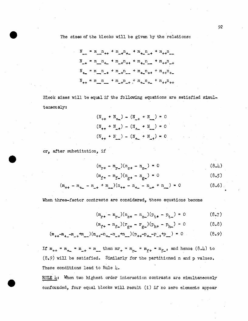
92
The sizes of the blocks will be given by the relations:
Block sizes will be equal if the following equations are satisfied simul-
taneously:
(N++ + N+_)
(N++ + N_+)
(N++ + N )
(N_+ + N ) = 0--(N+_ + N ) = 0-(N+_ + N_) = 0
or; after substitution, if
(m + - m )(n + - n ) = 0r r- s· s-
(mf + • mf_)(ng+ - ng_) = 0
(m++ - m+_ - m_+ + m_)(n++ - n+_ - n_+ + n ) = 0
When three-factor contrasts are considered, these equations become
(mr + - mr_)(ns + - ns_)(pt + - pt -) = 0
(rof + - mf_)(rg+ -rg_)(Ph+ - Ph-) = 0
(m++-m+__-m.+ -+m__ ) (n++-n+_-n_++n__ ) (P++-P+_-P_++p_) = 0
(8.4)
(8-5)
(8.6)
(8.7)
(8.8)
(8.9)
If m++ = m+_ = m_+ = m__ then roT+ ::: mr _ '" rof + ::: mf _, and hence (8.4) to
(8.9) will be satisfied. Similarly for the partitioned n and p values.
These conditions lead to Rule 4.
RULE 4: When two highest order interaction contrasts are simultaneously
confounded, four equal blocks will result (i) if no zero elements appear

93
in any coefficient vector of any factor in the two contrasts; and (ii) when
the first coefficient vector of the first contrast is partitioned according
to the first coefficient vector of the second contrast (or vice versa),
and the same process applied to the two corresponding coefficient vectors
of the other factors in the two confounding contrasts, the parts of at
least one of these partitioned coefficient vectors contain the same number
of elements.
Table 22 supplies the signs of the elements of the orthogonal poly-
nomial values for n = 2, 4, 6 and 8.
Table 22. Signs of the elements of the orthogonal polynomial vectors.
n = 2 n = 4 n = 6 n = 81 1 2 3 1 2 3 4 5 1 2 3 4 5 6 7
+ + - + - + - + ++ + + + + + - + - -+
+ + + - + + -+ + + + - - + + + + +
+ + + + - -+ + + + + + - + + +
+ + - - - - -+ + + + + + +
If the elements of each degree are partitioned in terms of the elements
of each of the other degrees, the relation n++ = n+_ = n_+ = n__ holds
when n is equal to 4. When n is equal to 8, the relation does not hold
for the partitionings 11 3, 115, 317, 51 7, but is true for all the other
partitionings. When n is equal to 2 or to 6, the relation does not hold.
It is also possible to obtain four equal-sized blocks in an
m x n experiment by the following procedure:

In general one can select any factor from (8.7) and a different
(a)
(b)
(c)
mr += mr _ and ng+ = ng_
ID++ = m_+ and ID+_ = m or n++ = n+_ and n_+ = n_
94
(8.10)
(8.11)
....--
one from (8.8) for (8.10) and then apply (8.11) accordingly. Hence one
can set up rule 4a.
RULE 4a. When two highest order interaction contrasts are s:ilnultaneously
confounded, four equal-sized blocks can also result if (i) no zero elements
appear in any coefficient vector; (ii) equality of positive and negative
elements in the original coefficient vectors follows (8.10); (iii) equality
of the m~B or n~~ follows (8.11); (iv) one can interchange factors as sug
gested in (c) above.
Rule 4aenables one to construct 6 level designs in four equal blocks.
8.3 Exper:ilnents in Equal Blocks With MainEffects Unconfounded
8.3.1 Two-factor experiments
Examination of Table II reveals that those two-factor experiments
in which the confounding of any highest order interaction contrast does
not confound main effect contrasts, also satisfy the rule for obtaining
two equal blocks. In all cases the number of levels of each factor must
be even; it any factor has an odd number of levels, at least one main effect
contrast will be confounded. In certain cases the number of positive ele-
ments must also equal the number of negative elements in the main effect
vector, as indicated below~

Confamdingcontrast
(uu)
(ue)
(eu)
(ee)
Requirements so that no main effectcontrasts will be confounded
m and n even
m even; n+ = n
n even; m.... = m
m =m-n =n+ -'.... -
95
/
Consider next the simultaneous confounding of any two highest order
interaction contrasts with corresponding subscripts not alike _ If
m = n = 0 and m = m and n = n (m andn both even), their generalizedo 0 + - +-
interaction will either be a single contrast of the same order or a linear
combination of contrasts of the same order (see Table 17) and hence no
main effect contrasts will be confounded because of this generalized inter-
action. By Rule 3, four equal blocks will result_ The homogeneous
bundles for various confounding patterns are indicated below_
Homogene aus bundle Sets of contrasts confounding this bundle
[EE] (uu,ul u1.); (ue,u1e], ); (eu,elul ); (ee,e1.e1.)
[EU] (uu,u],e1 ); (ue ,u1.ul ) ; (eu,e1 e1.); (ee,el u1.)
rUE] (uu,el u1.); (ue,elel ); (eu,ulul ); (ee,ule],)
[00] (uu,e], e1 ); (ue,elul ); (eu,ul el ); (ee ,ul U l )
8.3.2 Three-factor experiments
Examination of Table 15 reveals that those m x n x p experiments,
in which the confounding of any higher order interaction contrast does not
confound main effect contrasts, also satisfy the rule for two equal blocks.
The combination of factor levels in the confounding interaction contrasts
which will not result in confounding main effect contrasts are presented
below.

Confoundingcontrast
uuu
uue
uee
eee
Requirements so that no main effectcontrasts will be confounded
m, n and p even
m and n even
two or three of these: m. = m_,
96
The interaction contrasts which are confounded are presented in Table 15.
Consider finally the simultaneous confounding of any two highest
order interaction contrasts. From the left-hand column of the extension
of Table 18 to three factors, we see that no more than one pair of the
corresponding subscripts (out of the three) can be alike and still not
confound a main effect because of the generalized interaction.
Table 23 supplies the confounding contrasts of highest order of
an m x n x p experiment such that the simultaneous confounding of any
two--with not more than one pair of corresponding subscripts alike--wi11
yield four equal blocks without confounding main effect contrasts. To
distinguish between an odd and an even number of levels: affix an asterisk
to each of the letters corresponding with factors with an even number of
levels, but the number of positive and negative elements differ for at
least one contrast; affix an additional asterisk to the same letter if
the coefficient vector of the factor corresponding with that letter con-
tains the same number of positive as negative elements for all contrasts.
For instance, p will denote an odd number of levels; p* an even number of
levels, but some p+ f P_; p~ an even number of levels such that all

97
Table 23. Confounding contrasts of highest order not confounding main l/effects and yielding four equal blocks, when taken in pairs.=t
euu
eue
m x n~ x It*'
euu
eue
eeu
eee
euu
ueu
uue
uuu
m* x n~ x p*:*
euu
eue
uue
ueu
uee
uuu
17Notmore than one pair of corresponding subscripts shoud be alike;e.g., for the first column, A I A or BIB .
e e1 u U1
giNo asterisk denotes odd number of levels.* denotes even number, but n+ I n_ for at least one contrast.,. denotes even number and p+ = P_ for all contrasts.
Details for the ~ x nD x p** and m** x n*"* x p'** are not given in
Table 23, since in these cases all eight possible confounding contrasts
(uuu,uue, ••• ,eee) can be used.
Four equal blocks in which main effect contrasts are not confounded
will also be obtained when an appropriate three-factor and an appropriate
two-factor interaction contrast, with corresponding subscripts not alike,
are confounded simultaneously. Four equal blocks in which no main effect
contrasts are confounded will finally result when two appropriate two-
factor interaction contrasts, with all corresponding subscripts not alike
when both are not zero, are confounded simultaneously.
When two three-factor interaction contrasts are confounded simul-
taneously, the requirement of at least two pairs of corresponding sub-
scripts to be unlike cannot always be met in practice, with the result
that main effect contrasts will be confounded. In such cases it becomes
necessary to confound either one three-factor and one two-factor contrast

98
or two two-factor contrasts. Consider, for instance, the confounding of
(euu,e1 u1 e1 ) in an m x n4 x p~ experiment. If m :: 3, n* :: 2, p*"* :: 4,
the confounding contrasts will be (2lu,2le) and the generalized interaction
L( 20u ' ,0Ou ' ); by Table 18 [oro] will be confounded. If, however,
(21u,01e) or (20u,01e) are chosen as confounding contrasts, no main effect
contrast will be confounded.
By' Rule 2, three equal blocks can only result from the confounding
of a highest order interaction contrast when one of the factors has three
levels, and the coefficient vector of this factor in the confounding con
trast is of the first degree. If such is the case, however, Tables 11 and
15 show that main effect contrasts will be confounded. Hence it is im
possible to confound a polynomial oontrast and obtain experiments in three
equal blooks for whioh main effeot oontrasts are unoonfounded. Similarly
for the oase when six equal blooks are desired) here again, by Rule .3, one
of the faotors must have three levels.
From a praotioal point of view, one would be interested in oon
founded experiments in which the equal blook sizes are not too large, and
in whioh main effect oontrasts as well as first-order first degree inter
aot~on oontrasts and possibly seoond-order first degree interaction
contrasts (e.g., (110) or (111)] are unoonfounded.
As oan be expeoted from the extensive investigations undertaken by
Yates (19.37), Li (1944), Kempthorne (1952), Binet et al (1955) and other'
authors, most of the two-factor and three-faotor experiments whioh have
some or all of these desirable properties are already available ~n the
literature. The following designs, however, could not be found in the
literature and appear worthy of tabulation. Two of these experiments
are compared with ones suggested by 1i (1944) and analyzed from the degree
point of view by Binet et al (1955).

99
Table 24. New three-factor experiments in four equal blocks with maineffects unconfounded.
Type of Confounding Contrast confounded?experiment contrasts 110 101 011 III
4x 2 x 2 (201,210) No No Yes No
6x 2 x 2 (ell,u1 10) Yes Yes Yes No
8 x 2 x 2 (ell,e1 10) No No No No
4x4x2(2ul,220) No No No No(201,u1 20) No No No No
6x4x2 (e21,u1 01) No Yes No No
8 x 4 x 2 (eel,e1u1 1) No No No No
4x 2 x 2 1st repl- Yes Yes No NoLi(1944) 2nd repl. Yes No No Yes
3rd repl. No Yes No Yes
4x4x 2 1st repl. Yes No No NoLi(1944) 2nd repl. Yes No No No
3rd repl. No No No Yes
8.4 Confounding of Linear Combinations of Contrasts
In the previous section it was shown to be impossible to obtain
three equal blocks with main effects unconfounded when confounding a
single orthogonal polynomial contrast. With a 3 x 3 experiment, for
instance, the confounding of (A2 B1 ) will yield three equal blocks but
will confound B1 and Bli!; the confounding of (A1 B2 ) will yield three equal
blocks, but will confound A:L and Alii. The question arises whether it would
be possible to obtain a contrast equal to some linear combination of
orthogonal polynomial contrasts such that its confounding will leave main
effects free.

100
From the scheme below it can be seen that if such a contrast exists,
the signs of its elements must follow some such pattern as given in the
last two columns.
Alternative
Treatment Elements of contrasts (y = 1) signs of
combination ~B;a A2 B]. A:aB]. + A].B;a A;aBJ. - A].B;a AxBx
00 -1 -1 . -2 0 001 +2 0 +2 -2 +02 -1 +1 0 +2 0 +
10 0 +2 +2 +2 + +11 0 0 0 0 0 012 0 -2 -2 -2
20 +1 -1 0 -2 021 -2 0 -2 +2 +22 +1 +1 +2 0 + 0
It can be seen at once that our requirements will be met when
or
(8.13)
Confounding of (8012) will yield the I-component design, while con
founding of (8013) will yield the J-component design of Yates (1937) ..
These designs do not confound main effect contrasts ..
A similar investigation of the 33 experiment shows that the res-
pectiva confounding of the follOWing linear combinations of contrasts will
yield the replicates of Yates' (1937) balanced design in bocks of nine.
Again main effect contrasts are unconfounded.. The replicate numbers cor-
respond to the tabulation by Cochran and Cox (1950).

101
Replicate I: (AJ.BaCa ) + (AaB1C2 ) - (AaBaC1 ) + 3(A1B1C1 )
Replicate II: (A1BaCa ) + (AaB1Ca ) + (A B C ) - 3(,\B1C1 ):2 a 1
Replicate III: (~BaC:,) - (AaB1Ca ) + (AaBaC1 ) + 3(~BJ.CJ.)
Replicate IV: -(~BaC2) + (AaB1Ca ) + (AaBaC1 ) + 3(~~C1)
Similarly experiments of the type 33 x q¥f and 32 x p~ X q*" can be
arranged into six equal blocks without confounding main effects by the
simultaneous confounding of the linear combination (8.12) or (8.13) and
an appropriate two-factor interaction contrast. Thus, for instance, we
have the following sets of confounding contrasts for certain experiments.
3x3x 3 x q'* : (XXOO, 002u )
3x 3x 3xq~~ · (xXOO,002u) or (xXOO,002e)•
3x 3 x p'*' x q* · (xXOO, OOuu )•
3x 3 x p~ x q~ · (XXOO, oOnu ) or (xXOO, OOeu )•
Binet et al (195'5') devote considerable space to the 32 x 22 experi-
ment in blocks of 12; 12 new plans were developed and the confounding pattern
for a design of Li (1944) is presented. A design in six blocks of six units
each, obtained by simultaneously confounding the contrasts (xXOO) and (0011),
is identical to the one developed by Kempthorne (195'2) and confounds,
inter alia, ~B]., C]. D]., A].B]. 01D].. From a degree point of view, this design
appears to be useful; when the experimental material is rather variable;
it may be better than the design in blocks of 12.
8.5' Balanced oonfounding
Consider the 3 x 2 x 2 experiment. By Rule 1 and Table 14, oonfound-·
ing of the oontrast (211) will yield two equal blocks; contrast (011) will
be confounded, but no others. This blocking arrangement is identical to

102
Replicate II of the plan given by Oochran and Oox (1950). The confounding
scheme for this blocking arrangement is given in the first line in the
body of the scheme below:
Oonfounding A B 0contrast 0 1 2 01 01
211 + - + + +
xlI - + + + +
XII + + - - + - +
Let (xlI) and (XII) be contrasts, the signs of which are as in
dicated above. The confounding of (xlI) yields Replicate I, and the con
founding of (XII) yields Replicate III of the balanced design supplied by
Oochran and Oox (1950). Let x' be the row vector (-2,1,1) and X' the row
vector (1,1,-2). If P denot es the orthogonal polynomial of degree r then,r
when x and X are expressed in terms of P1 and Pa for m = 3, we find
x = (JP1 -P2 )/2
X = -(JP1 +Pa )/2
Hence
(xlI) = (J~B101 - A2~01 )/2
(XII) = -(3A1B101 + AaBa01 )/2
This result shows that a balanced group of sets for the 3 x 22
experiment can be obtained by confounding the required highest order
interaction contrast in one replicate, and those linear combinations of
highest order interaction contrasts derived from the signs of the required
contrast in two other replicates.

103
In practice one would obtain this results as follows: interchange
levels ° and 1 of the first factor in Replicate II to obtain Replicate I,
and interchange levels 1 and 2 of the first factor in Replicate II to
obtain Replicate III. Similar results can be derived for a 3 x 2n experi
n-l Gment in equal blocks of size 3 x 2 • eneralization is possible. Hence
we have shown that linear combinations of orthogonal contrasts play an
important part in obtaining balanced sets of treatment combinations; how-
ever, this subject is not pursued further in this thesis.

104
CHAPTER 9
Summary, Conclusions and Suggestions for Future Research
901 Summary and Conclusions
The survey of literature reveals that for all factors of a factorial
experiment 'With the same prime number (or power of a prime number) of levels,
results from Finite Group Theory can be employed to confound the experiment
into equal blocks, or into fractions, leaving main effects and some lo'Wer
order interactions unconfounded. For factors with different numbers of
levels, no such general theory exists.
In many experimental situations it 'Would be desirable to confound
higher degree rather than higher order contrasts. A general mathematical
technique, based on conformable partitioning of the coefficient matrices
of orthogonal contrasts, was developed to obtain confounded designs for
both the symmetrical and asymmetrical cases. This approach not only leads
to designs required from the degree point of view, but reproduces most of
the designs based on the confounding of order components. By defining the
positive and negative signs of the 'matrix elements and the zero elements
of a contrast as block indicators, it 'Was shown that confounding of a
contrast with blocks corresponds mathematically to a partitioning of the
coefficient matrix of the contrast according to the block indicators.
The study of the confounding pattern of a contrast was thus reduced to a
mathematical examination of the values of the traces of conformably par
titioned coefficient matrices.
Using this technique, certain general theorems were derived in
Part I. Considering the confounding of a single contrast at a time, it
was shown that the confounding of a contrast of lower order does not con
found any contrast of higher order. Conditions were established for the

105
case in which the confounding of a contrast of higher order does not con
found any contrast of lower order, and for the case in which the confound
ing of a contrast of given order does not confound contrasts of the same
order. These theorems led to the definition of the heterogeneous bundle
of a confounding contrast, such a bundle consisting of all the contrasts
confounded by that contrast. When two contrasts are confounded simul
taneously, it is shown that their symbolic product yields another
heterogeneous bundle, that of the generalized interaction.
In Part II these general results are specialized to the orthogonal
polynomial contrasts. Tables are presented of the heterogeneous bundles
of confounding contrasts of highest order. An easy rule for determining
the heterogeneous bundle of any given contrast was found, this rule being
a convenient arithmetization of the consequences of the various theorems.
A rapid procedure to determine the coefficients of the block constants in
the expectation of the confounded contrasts is demonstrated. The general
ized interaction of two polynomial contrasts was reduced to a linear
combination of polynomial contrasts, and theorems were developed to
determine the confounding status of these contrasts. The rule to deter
mine heterogeneous bundles was generalized. Conditions necessary to
obtain equal blocks, when one or more contrasts of highest order are
confounded, but main effects are not confounded, were established.
These conditions ll?ad to new single-replicate three-factor experiments
in four equal blocks in which main effects are unconfounded.
10.2 Further Research Needed
Since this thesis dealt with a field of research rather than with
a single topic, many single topics require further elaboration.

106
1 0 A complete discussion of partial confounding (in the sense of
this thesis); including a method of estimating all pertinent contrasts
and their standard errors.
20 A systematic search for new four- and five-factor confounded
designs in equal blocks with main effects unconfounded, using the short
cut methods developed in this thesis.
30 A .fuller treatment of the theory of confounding linear combina
tions of orthogonal contrasts, along the lines proposed for single
orthogonal contrasts.
40 The use of unequal-sized blocks.
5. The development of a comprehensive theory of fractional repli
cation, based on signs of contrasts, with special emphasis on the asym
metrical case.
6.. The extension of the present theory of confounding based on
the signs only of contrasts, to one based on both the signs and types of
elements of the contrasts; hence, the extension of the system of block
indicators (-,+,0) to something like (-e,+e,-u,+u,O), where e denotes
an even element and u an odd element.

107
LITERATURE CITED
Aitken, A. c. 1933. On the graduation of data by the orthogonalpolynomials of least squares. Proc. Roy. Soc. Edinburgh 21: 54-78,
Allan, F. E. 1930. The general form of the orthogonal polynomialsfor simple series with proofs of their simple properties.Proc. Roy. Soo. Edinburgh 2Q: 310-320.
Anderson, R. L. 1953. Reoent advances in finding best operatingoonditions. Jour. Amer. Stat. Assn. 48: 789-798.
Anderson, R. L. 1957. Complete faotorials, fractional factorialsand confounding. Proc. Symp. Design of Industrial Experiments,North Carolina State College (in press).
Anderson, R. L., and Houseman, E. E. 1942. Tables of orthogonalpolynomial values extended to n =104. Iowa State College,Agr. Expt. Sta. Res. Bull. 297.
Barnard, M. M. 1936. An enumeration of the confounded arrangementsin the 2 x 2 x 2 •.• factorial designs. Jour. Roy. Stat. Soo.Supple 2: 195-202.
Binet, F. E., Leslie, R. T., Weine~, S., and Anderson, R. L. 1955.Analysis of confounded faotorial experiments in singlereplications. North Carolina Agr. Expt. Sta. Teoh. Bull. 113.
Bose, R. C. 1938. On the application of the properties of Galoisfields to the construction of hyper Graeco-Latin squares.Sankhya 2: 323-338.
Bose, R. C. 1947. Mathematical theory of symmetrioal factorial designs.Sankhya ~: 107-166.
Bose, R. C. 1950. Mathematics of faotorial designs. Proe. International Congress of Mathematioians 1950: 543-548.
Bose, R. C., and Kishen, K. 1940. On the problem of oonfounding inthe general symmetrical factorial design. Sankhya 2: 21-36.
Box, G. E. P. 1952. Multi-factor designs of first order.Biometrika ~: 49-57.
Box, G. E. P. 1954. The exploration and exploitation of responsesurfaoes: Some general oonsiderations and examples.Biometrics 10: 16-60.
Box, G. E. P., and Hunter, J. S. 1954. Multi-faotor experimentaldesigns. Inst. of Statistics Mimeo Series No. 92. NorthCarolina State College, Raleigh.
Box, G. E. P., and You1e, P. V. 1955. The Exploration and exploitationof response surfaces: An example of the link between the fittedsurface and the basic mechanism of the system. Biometrics 11:287-323.

108
Box, G. E. P., and Wilson, K. B. 1951. On the experimental attainmentof optimum conditions. Jour. Roy. Stat. Soc., Ser. B, 13: 1-45.
Brownlee, K. A., Kelly, B. K., and Loraine, P. K. 1948. Fractionalreplication arrangements for factorial experiments with factorsat two levels. Biometrika 35: 268-276.
Chinloy, T., Inne:s, R. F., and Finney, D. J. 1953. An example of fractional replication in an experiment on sugar cane manuring. Jour.Agr. Sci. 43: 1-11.
Cochran, W. G., and Cox, G. M. 1950. Experimental designs. John Wileyand Sons, New York.
Daniel, C. 1956. Fractional replication in industrial research. hoc.Third Berkeley Symposium on Math. Stat. and Prob. 2,:
Davies, O. L. (Ed.) 1954. Design and analysis of industrial experiments.Oliver and Boyd, Edinburgh and London.
Davies, O. L., and Hay, W. A. 1950. The construction and use of fractionaldesigns in industrial research. Biometrics 2: 233-249.
DeLury, D. B. 1950.up to n = 26.
Values and int egrals of the orthogonal polynomialsUniversity of Toronto Press.
Esscher, M. F. 1920. Uber die Sterblichkeit in Schweden. Medd.franLunds Astron. Obser. Ser. 2, No. ,23.
Esscher, M. F. 1930. On graduation according to the method of leastsqiiaresby means of c eTta.in polynomials. ForsakringsaktiebolagetSkandinavia, Festskrift. Stockholm.
Finney, D. J. 1945. The fractional replication of factorial experiments.Ann. Eugenics g:29l-301.
Finney, D. J. 1946. Fractional replication. Jour. Agr. Sci. ~: 184-191.
Fisher, R. A. 1921. Studies in crop variation I.the yield of dressed grain from Broadbalk.107-135.
An examination ofJour. Agr. Sci. 11:
Fisher,R. A. 1924.at Rothamst ed.
The influence of rainfall on the yield of wheatPhil.Trans. Roy. Soc. London B2l3: 89-142.
Fisher, R. A. 1926. The arrangement of field experiments. Jour.Ministry of Agr. 33: 503-513-
Fisher, R. A. 1935. The design of experiments. Oliver and Boyd,Edinburgh, First ed.
Fisher, R. A. 1942. The theory of confounding in factorial experimentsin relation to the theory of groups. Ann. Eugenics 11: 341-353.

109
Fisher, R. A. 1945. A system of confounding for factors with more thantwo alternatives, giving completely orthogonal cubes and higherpowers. Ann. Eugenics 12: 283-290.
Fisher, R. A., and Wishart, J. 1930. The arrangement of field experimentsand the statistical reduction of the results. Imperial Bureau ofSoil Science. Tech. Gomm. No. 10.
Fisher, R. A., and F. Yates. 1938. Statistical tables. Oliver andBoyd, Edinburgh. First Ed.
Gram, J. P. 1915.funktionen.
Uber partie11e Ausg1eichung mittelst Orthogona1Mitt. Ver. schweiz. Versich. Math. 1£: 41-73.
Jordan, C. 1929. Sur la determination de 1atendence secu1airedesgrandeurs statistiques par 1a methode des moindres carres. Jour.de 1a Soc. Hongroise de Stat. I: 567-588.
Jordan, C. 1932. Approximation and graduation according to the principleof least squares by orthogonal polynomials. Ann. Math. Stat.1: 257-333.
Kempthorne, O. 1947. A simple approach to confounding and fractionalreplication in factorial experiments. Biometrika~: 255-272.
Kempthorne, O. 1952. The design and analysis of experiments. JohnWiley and Sons, New York.
Kitagawa, T., and Mitome, M. 1953. Tables for the design of factorialexperiments. Baifukan Co., Ltd., Tokyo.
Li, J. C.-R. 1844. Design and statistical analysis of so:meconfoundedfactorial experiments. Iowa State College Agr. Exp. Sta. Bull.333.
Lorenz, P. ,1931. Der Trend. Vierte1jahrshefte zur Konjunkturforschung.Sonderheft 21.
Nair, K. R. 1938. On a method of getting confounded arrangements inthe general symmetrical type of experiments. Sankhya 11: 121-138.
Nair, K. R. 1940.experiment s •
Balanced confounded arrangements forthe5n type ofSankhya ~: 57-70.
Nair, K. R., and Rao, C. R. 1948. Confounding in asymmetrical factorialexperiment s • Jour. Roy. Stat. Soc. Sar. B!2: 109-131.
Pearson, E. S., and Hartley, H. o. 1954. Biometrika tables forstatisticians. Vol. 1. Cambridge University Press.
P1ackett, R. L., and Burman, J. P. 1946. The design of optimum multifactor experiments. Biometrika..12.: 305-325.

110
Poincare, H. L. 1896. Calcu1 des probabilitieSl. Hermann et Cie, Paris.
Tchebycheff, P. L. 1859. Sur l'interpo1ation par 1a methode des moindrescarres. Oeuvres Completes, Gauthier-Villars, Paris.
Thompson, H. R. 1952. Factorial design with small 'olocks. New ZealandJour. Sci. and Technol. B33: 319-344.
Thompson, H. R., and Dick,I. D. 1951. Factorial designs in small blocksderived from orthogonal latin squares. Jour. Roy. Stat. Soc.B13: 126-130.
Van der Reyden, D. 1943. Curve fitting by the orthogonal polynomials ofleast squares. Onderstepoort J. Vet. Sci. ,gQ: 355-404.
Yates, F. 1933. The principles of orthogonality and confounding inreplicated experiments. Jour. Agr. Sci. 23: 108-145.
Yates, F.2:
1935. Complex experiments.181-247.
Jour. Roy. Stat. Soc. Supple
Yates, F. 1937. The design and analysis of factorial experiments.Imperial Bureau of Soil Sci. Tech. Comm. No. 35.