NAS A/TP--2000-210386

The Use of Ferrofluids to

Model Materials Processing(MSFC Center Director's Discretionary Fund Final Report,

Project No. 98-12)

F. Leslie

Marshall Space Flight Center, Marshall Space Flight Center, Alabama

N. Ramachandran

Universities Space Research Association, Huntsville, Alabama

National Aeronautics and

Space Administration

Marshall Space Flight Center • MSFC, Alabama 35812

July 2000

https://ntrs.nasa.gov/search.jsp?R=20000092062 2018-06-14T10:31:58+00:00Z

Acknowledgments

This work was supported by funding from NASA MSFC Center Director Discretionary Fund. The work by N. Ramachandran

was done under the auspices of the Alliance for Microgravity Materials Science and Applications through NASA contract

NCC8-66. The authors would also like to acknowledge Mr. Charles Sisk for his efforts in measuring the magnetic fieldand Soyoung Cha for his assistance with the camera calibration.

Trademarks

Trade names and trademarks are used in this report for identification purposes only. This usage does not constitute an official

endorsement, either expressed or implied, by the National Aeronautics and Space Administration.

NASA Center for AeroSpace Information7121 Standard Drive

Hanover, MD 21076-1320

(301) 621-0390

Available from:

National Technical Information Service

5285 Port Royal Road

Springfield, VA 22161(703) 487-4650

ii

TABLE OF CONTENTS

.

2.

3.

4.

APPENDIX

APPENDIX

INTRODUCTION .........................................................................................................................

THEORETICAL CONSIDERATIONS ........................................................................................

EXPERIMENT CONFIGURATION ............................................................................................

PHOTOMETRIC ANALYSIS .......................................................................................................

A--FERROFLUID DENSITY .....................................................................................

B---CONCENTRATION GRADIENTS .......................................................................

B.1 General Case ..........................................................................................................................

B.2 Linear Gradient ......................................................................................................................

B.3 Exponential Gradient .............................................................................................................B.4 The Test Cell ..........................................................................................................................

REFERENCES ................................................................................................................................

1

5

9

11

19

21

21

22

23

24

25

iii

LIST OF FIGURES

l, Magnetization curve of ferrofluid used in this study ..................................................... 7

. Measurements of the magnetic field in the vertical plane of the experiment ................ 8

. Arrangement of the experiment apparatus ..................................................................... 10

.

.

Schematic for development of the absorption equation ................................................ 12

The extinction coefficient versus concentration measured at

several wavelengths using a spectrophotometer ............................................................ 14

. Calculation of the extinction coefficient for filtered and unfiltered light ...................... 15

. A comparison of the photometrically measured concentration

versus the known (prepared) values ............................................................................... 15

. The theoretical reduction of intensity with increasing concentration ............................ 16

. Test cell containing a concentration gradient stabilized by an overhead

magnetic field ................................................................................................................ 17

10.

11.

12.

13.

The measured and theoretical distribution of concentration in the test cell .................. 17

Variation of density with particle concentration ............................................................ 20

Gradient former ............................................................................................................. 21

Test cell .......................................................................................................................... 24

iv

LIST OF TABLES

°

2.

Prepared (known) concentrations .....................................................................................

Fluid properties at various concentrations .......................................................................

14

19

ABBREVIATIONS AND SYMBOLS

al(x,y)

_(x,y)

S

11o

V

P

Po

a

b

C

CK

Cmo

C_

Cv

g

H

lo(x,Y)

lo(x,y)

k

M

attentuation coefficient of first wall

attentuation coefficient at second wall

extinction coefficient of the ferrofluid

density coefficient

diameter of magnetic particles

permeability of free space

kinematic viscosity

fluid density

density at O=O

volume fraction of solid magnetic particles

test cell width

test cell depth

concentration

known constant fluid concentration

initial concentration in the mixer

concentration in the supply syringe

volume concentration of the ferrofluid

gravity

strength of the applied magnetic field

initial (non-uniform) intensity

image intensity at D

digital array of known concentration

Boitzmann's constant

magnetization of the fluid

vi

ABBREVIATIONS AND SYMBOLS (Continued)

Ms

P

T

V

Vy_n_t

Vm

Vmo

Pro

I: t

magnetization of the bulk magnetic solid

maximum (saturation) magnetization

pressure

absolute temperature

velocity

final volume of fluid in the test cell

volume of the mixer

initial volume of the mixer

initial reservoir volume

total volume deployed

vii

TECHNICAL PUBLICATION

THE USE OF FERROFLUIDS TO MODEL MATERIALS PROCESSING

(MSFC Center Director's Discretionary Fund Final Report, Project No. 98-12)

1. INTRODUCTION

A great number of crystals grown in space are plagued by convective motions, which contribute to

structural flaws. The character of these instabilities is not well understood but is associated with density

variations in the presence of residual gravity and g-jitter. As a specific example, past mercury cadmium

tellurium (HgCdTe) crystal growth space experiments by Gilies et al. I indicate radial compositional asym-

metry in the grown crystals. In the case of HgCdTe, the rejected component into the melt upon solidifica-

tion is mercury tellurium (HgTe) which is denser than the melt. The space-grown crystals indicate the

presence of three-dimensional flow with the heavier HgTe-rich material clearly aligned with the residual

gravity (0.55-1.55 lag) vector. This flow stems from multicomponent convection, namely, thermal and

solutal buoyancy-driven flow in the melt. A model, fluids experiment to study this problem in space

requires the rapid development of a concentration (density) gradient which is difficult to establish in the

absence of a stabilizing gravitational field. An important objective of this study is to evaluate the feasibility of

using a magnetic fluid to study this phenomenon. Once the effectiveness of a magnetic field in stabilizing

the concentration gradient is established, the developed techniques can be utilized in the design of a space

experiment to study the crystal growth instability problem.

When a magnetic or ferrofluid is placed in an appropriate magnetic field, the induced body force

can be utilized for fluid manipulation. This technique is also significant in its potential for greatly improv-

ing the performance and lowering the cost of spacecraft thermal management systems. For example, terres-

trial electronic systems often rely on gravity driven natural convection for heat rejection. In the reduced

gravity environment of space, (i.e., Earth orbit, Moon, Mars), natural convection heat-transfer rates are so

diminished that innovative solutions are required to efficiently reject heat and maintain the system at an

acceptable temperature. The ease of essentially dialing in the required body force (gravity level) holds the

promise of active thermal control (dynamically enhancing or suppressing convective heat transfer rates) of

space systems.

Artificial ferrofluids are typically colloidal suspensions of extremely small ferrite particles that

have been treated with a surfactant to prevent clumping and settling, (see Odenbach 2 for experiments

allowing for the demixing of the magnetic particles and the resulting forced diffusion that drives convection).

Although a multiphase mixture at the microscopic scale, the nearly uniform dispersion of very small

particles permits ferrofluids to be well represented by a continuum model. Neuringer and Rosensweig 3

present the fundamental hydrodynamic equations describing the flow of a ferrofluid and highlight the

primary phenomena arising from the coupling between an imposed magnetic field and the fluid flow.

Most applications of ferrofluids involve their use in very small-scale devices or as a thin film that is

subjected to magnetic, gravitational, and heating effects. Highly successful applications of this

technology include printers, pumps, clutches, brakes, and seals. Driven by these applications, research has

focused on interfacial stability limits, magnetization effects on buoyancy and thermocapillary

convection, fluid flow in simple planar or cylindrical geometries, and the deformation of simple surfaces

and drops. Zelazo and Melcher 4 studied the dynamics and stability of ferrofluids with particular emphasis

on surface interactions. They found that, although the nonlinear magnetization characteristics of ferrofluids

complicate wave dynamics and stability, the magnetic coupling with homogeneous fluids is confined to

interfaces. They also noted that the magnetic force can provide a stabilizing effect on a Rayleigh-Taylor

instability. Finlayson 5 studied the convective instability of a ferrofluid layer heated from below in the

presence of a uniform vertical magnetic field and found that the magnetic field can suppress buoyant

convection. Bashtovoi, and Krakov 6 and Bashtovoi 7 examined the stability of magnetizable liquid layers

and jets in the presence of uniform magnetic fields. They showed that the magnetic forces lead to nonuni-

form pressure distributions, which can have a significant effect on the stability of the flow. Bashtovoi 8 also

studied the problem of magnetic convection of a ferrofluid heated from below and found the problem

similar to the classic Rayleigh instability of a classical fluid in the presence of a gravitational field alone.

The additional magnetic body force resulted in a more comprehensive Rayleigh number containing

magnetic properties that predicts the onset of convection. The magnetic Rayleigh-Brrnard problem was

also studied by Schwab et al. 9 and by Stiles and Kagan. 10 One of the few studies involving non-equilibrium

magnetization was performed by Rosensweig et al.ll who examined the flow of a ferrofluid in a rotating

magnetic field.

Nakatsuka et al. 12 performed experiments to study the heat-transfer rate of a simple heat siphon in

a magnetic field. Their data show that the heat-transfer rate of a vertical wire in a magnetic fluid can be

enhanced with the application of a magnetic field. Aihara et al. 13 numerically modeled the convection of a

magnetic fluid flowing through a circular tube with an axial magnetic field. They showed that as the Reynolds

number of the flow decreased, the magnetic force becomes more effective in transporting the heat. More

recently, Zebib 14 examined theoretically an internally heated cylindrical shell with a radial magnetic field

acting on a ferrofluid fluid. His calculations determined the critical magnetic Rayleigh number for the

onset of convection in this geometry within the constraints of his model. The convection took the form of

a number of counter-rotating rolls in the radial azimuthal plane transferring heat from the inner cylinder to

the outer wall.

The study of naturally occurring paramagnetic and diamagnetic fluids has not been as extensive as

the study of ferrofluids because their magnetization is so weak that forces induced by the presence of a

magnetic field are usually negligible with respect to gravitational forces. Notable exceptions are liquid

coolant lines in plasma confinement systems and particle accelerators where exceptionally strong

magnetic fields occur. Berkovsky and Smirnov 15 developed a theoretical framework for mathematically

modeling these flows which utilizes the same basic equations and boundary conditions that were

developed for the ferrofluid studies.

There have been very few experiments with magnetic heat transport in a reduced gravity environ-

ment. HOrsten et al. 16 flew an experiment in a TEXUS sounding rocket that examined the convection of a

magnetic fluid inside a cylindrical shell with gradients of the temperature and magnetic fields in the radial

direction. Results showed radial-azimuthal convection cells as anticipated, although only two appeared

2

instead of the expected eight. Odenbach _7also conducted experiments in low-gravity using a drop tower. In

spite of the short duration of low gravity, his experiments showed a critical magnetic Rayleigh number of

1820+100 needed for the onset of magnetic convection in a cylindrical shell. Odenbach _8,repeating the

experiments using a sounding rocket, obtained similar results.

In summary, although the effect of a magnetic field on the flow of a ferrofluid or a paramagnetic

fluid has been under study for >35 yr, understanding of this influence and its interaction with competing

forces such as gravity and surface tension is still in its infancy. Understanding of the combined effect of all

these forces on heat transfer is even less developed. The investigations have been primarily

small-scale experiments in a normal gravity environment with the addition of a few recent experiments that

used a reduced gravity environment to help expose the relationships between the competing influences.

The present study examines a technique that may be useful for studying instabilities which plague

crystal growth experiments in space. In these experiments, there is an exponential distribution of species

concentration in the region close to the crystal. When these density variations are acted upon by the

residual gravity (g-jitter), flow instabilities develop which impact the growth process. To study these

instabilities in a separate, controlled experiment, a concentration gradient would have to be artificially

established in a timely manner as an initial condition. This is generally difficult to accomplish in a

microgravity environment because the momentum of the fluid injected into a test cell tends to swirl around

and mix. However, the use of a magnetic fluid would allow it to be held in position during deployment and

then released by switching off the magnetic field before starting the experiment. The following describes a

technique for such a deployment and measurement of the resulting concentration field.

3

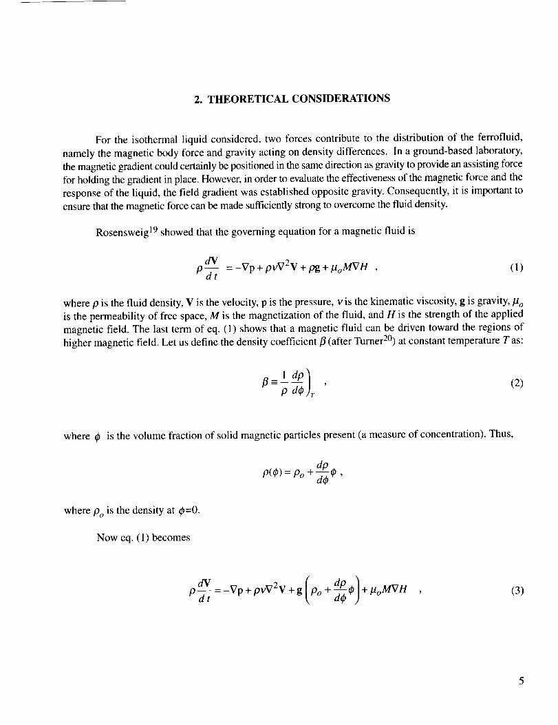
2. THEORETICAL CONSIDERATIONS

For the isothermal liquid considered, two forces contribute to the distribution of the ferrofluid,

namely the magnetic body force and gravity acting on density differences. In a ground-based laboratory,

the magnetic gradient could certainly be positioned in the same direction as gravity to provide an assisting force

for holding the gradient in place. However, in order to evaluate the effectiveness of the magnetic force and the

response of the liquid, the field gradient was established opposite gravity. Consequently, it is important to

ensure that the magnetic force can be made sufficiently strong to overcome the fluid density.

Rosensweig 19 showed that the governing equation for a magnetic fluid is

dVp-z- = -Vp + pvV2V + pg + IIoMVHdt

(1)

where p is the fluid density, V is the velocity, p is the pressure, v is the kinematic viscosity, g is gravity,/.t o

is the permeability of free space, M is the magnetization of the fluid, and H is the strength of the applied

magnetic field. The last term of eq. (1) shows that a magnetic fluid can be driven toward the regions of

higher magnetic field. Let us define the density coefficient fl (after Turner 2°) at constant temperature T as:

(2)

where O is the volume fraction of solid magnetic particles present (a measure of concentration). Thus,

P(¢) = Po + -_ ¢ ,

where Po is the density at @=0.

Now eq. (1) becomes

P--_=-Vp+pvV2V+g Po + @ +11o MVH (3)

5

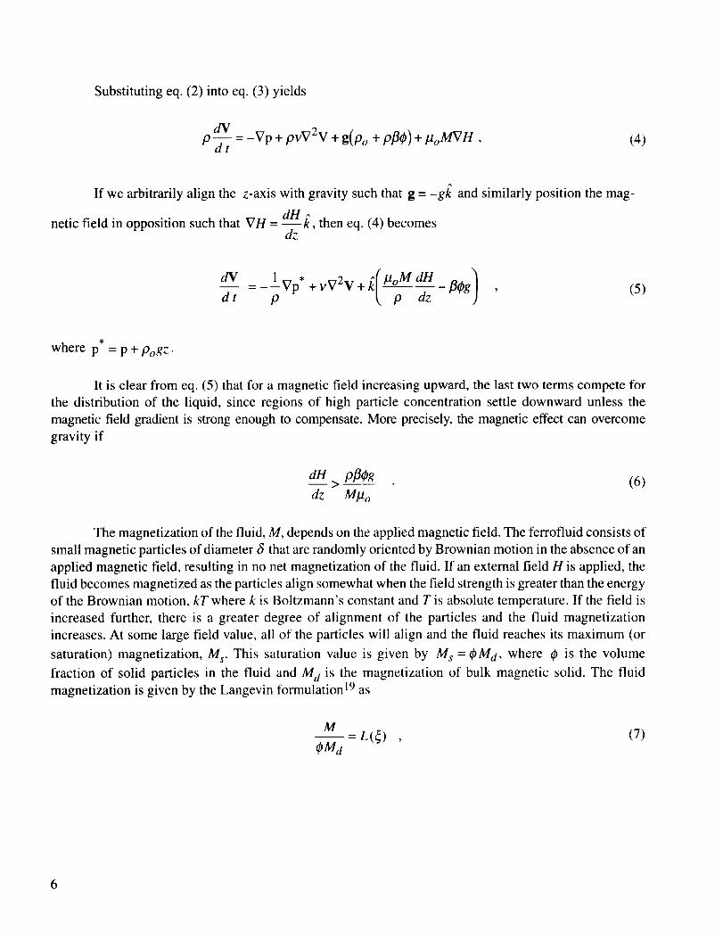
Substitutingeq.(2) into eq.(3) yields

dV

P-d_-t = -Vp + pvV2V + g(po + pfleP) + Po MVH , (4)

If we arbitrarily align the z-axis with gravity such that g = -g/_ and similarly position the mag-

netic field in opposition such that VH = drift, then eq. (4) becomesdz

- p Vp*+vv2V+/_ P dz flCg (5)

where p = p + PogZ.

It is clear from eq. (5) that for a magnetic field increasing upward, the last two terms compete for

the distribution of the liquid, since regions of high particle concentration settle downward unless the

magnetic field gradient is strong enough to compensate. More precisely, the magnetic effect can overcome

gravity if

dH pflCg-- >- (6)dz Mpo

The magnetization of the fluid, M, depends on the applied magnetic field. The ferrofluid consists of

small magnetic particles of diameter _ that are randomly oriented by Brownian motion in the absence of an

applied magnetic field, resulting in no net magnetization of the fluid. If an external field H is applied, the

fluid becomes magnetized as the particles align somewhat when the field strength is greater than the energy

of the Brownian motion, kT where k is Boltzmann's constant and T is absolute temperature. If the field is

increased further, there is a greater degree of alignment of the particles and the fluid magnetization

increases. At some large field value, all of the particles will align and the fluid reaches its maximum (or

saturation) magnetization, M s. This saturation value is given by M s = ¢pM d, where q_ is the volume

fraction of solid particles in the fluid and M d is the magnetization of bulk magnetic solid. The fluid

magnetization is given by the Langevin formulation 19 as

M _ L(_) , (7)CMa

6

where L(_) = coth(_) - 1 and _ = n" ll°"l'IdH_3"". Thus the requirement for dominance of the magnetic6 kT

force in the fluid over gravity becomes

dH pfl g-- > (8)dz MdLC )l.t o

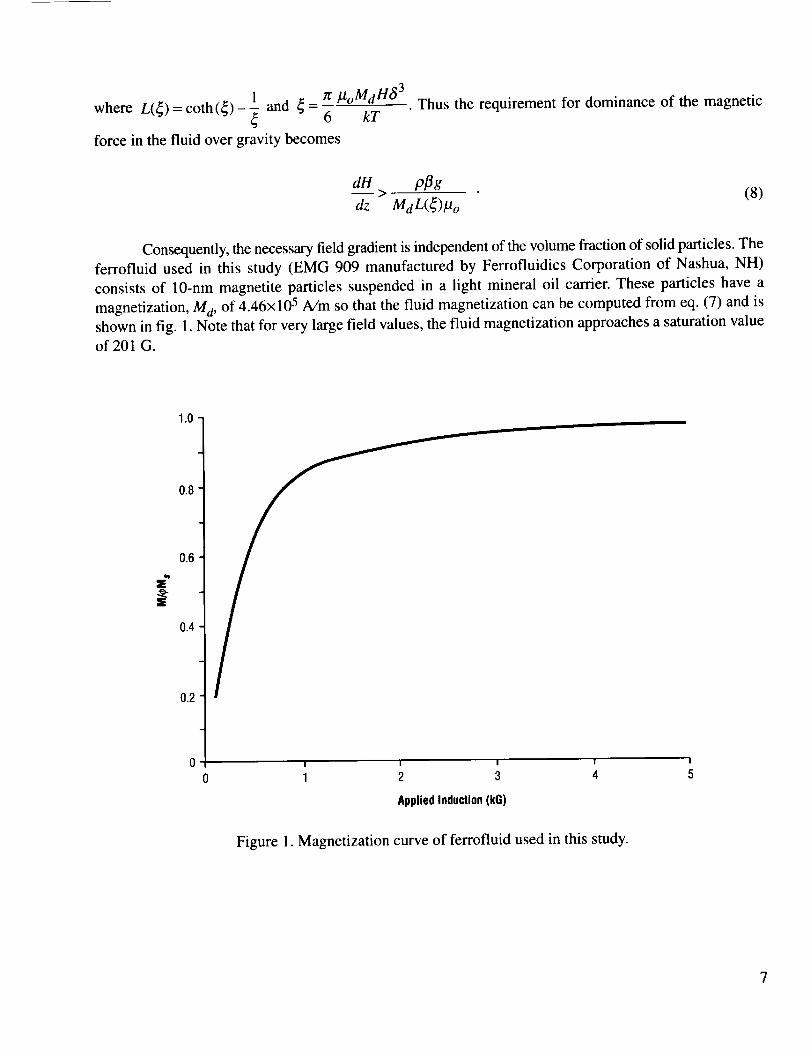
Consequently, the necessary field gradient is independent of the volume fraction of solid particles. The

ferrofluid used in this study (EMG 909 manufactured by Ferrofluidics Corporation of Nashua, NH)

consists of 10-nm magnetite particles suspended in a light mineral oil carrier. These particles have a

magnetization, M d, of 4.46× 105 A/m so that the fluid magnetization can be computed from eq. (7) and is

shown in fig. 1. Note that for very large field values, the fluid magnetization approaches a saturation valueof 201 G.

1.0

0.8

z

E

0.4

0.2

I I I I I

0 1 2 3 4 5

AppliedInduction(k6)

Figure 1. Magnetization curve of ferrofluid used in this study.

7

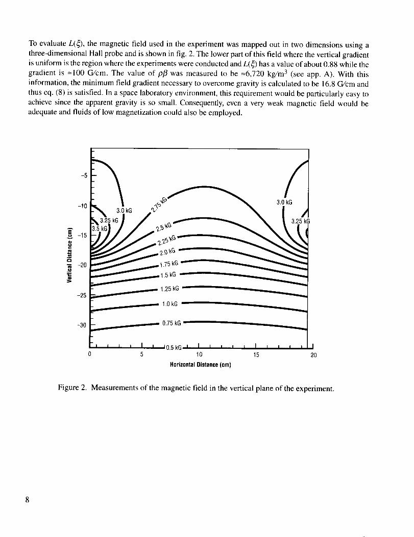
To evaluateL(_), the magnetic field used in the experiment was mapped out in two dimensions using a

three-dimensional Hall probe and is shown in fig. 2. The lower part of this field where the vertical gradient

is uniform is the region where the experiments were conducted and L(_) has a value of about 0.88 while the

gradient is =100 G/cm. The value of ,0]3 was measured to be =6,720 kg/m 3 (see app. A). With this

information, the minimum field gradient necessary to overcome gravity is calculated to be 16.8 G/cm and

thus eq. (8) is satisfied. In a space laboratory environment, this requirement would be particularly easy to

achieve since the apparent gravity is so small. Consequently, even a very weak magnetic field would be

adequate and fluids of low magnetization could also be employed.

-25 125 kG

1.0 kG

-30 0.75kG

0.5kG ' I J I , i I I I I I I

0 5 10 15 20

HorizontalDistance(cm)

Figure 2. Measurements of the magnetic field in the vertical plane of the experiment.

8

3. EXPERIMENT CONFIGURATION

The primary objective of this effort is to develop a method for quickly producing an exponential

gradient applicable to space experiments. By demonstrating this technique on the ground using a strong

magnetic field to overcome gravity, we can be assured that this method would be relevant to space systems

using a substantially weaker field.

A gradient former was used to produce the desired concentration distribution. It consists of a dual

syringe system, with one syringe containing pure solvent and the other the solute solution. By deploying

two liquids in different proportions into a mixing chamber and eventually into the test cell, precise

gradients ranging from linear to exponential can be realized within minutes (see app. B). This mechanism

works well in terrestrial laboratories where gravity assists in maintaining a stable stratification. In low gravity,

however, there is no restoring force to prevent swirling of the fluid as it is introduced into a test cell. This

jetting effect would immediately mix the liquid.

One way of stabilizing the required solute gradient is by using a magnetic fluid and a controlling

magnetic field to provide the required body force in the gradient former arrangement. A practical imple-

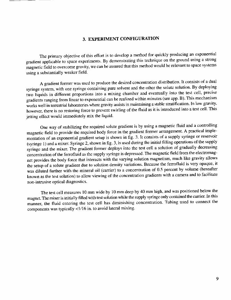
mentation of an exponential gradient setup is shown in fig. 3. It consists of a supply syringe or reservoir

(syringe 1) and a mixer. Syringe 2, shown in fig. 3, is used during the initial filling operations of the supply

syringe and the mixer. The gradient former deploys into the test cell a solution of gradually decreasing

concentration of the ferrofluid as the supply syringe is depressed. The magnetic field from the electromag-

net provides the body force that interacts with the varying solution magnetism, much like gravity allows

the setup of a solute gradient due to solution density variations. Because the ferrofluid is very opaque, it

was diluted further with the mineral oil (carrier) to a concentration of 0.5 percent by volume (hereafter

known as the test solution) to allow viewing of the concentration gradients with a camera and to facilitate

non-intrusive optical diagnostics.

The test cell measures 10 mm wide by 10 mm deep by 40 mm high, and was positioned below the

magnet. The mixer is initially filled with test solution while the supply syringe only contained the cartier. In this

manner, the fluid entering the test cell has diminishing concentration. Tubing used to connect the

components was typically < 1/16 in. to avoid lateral mixing.

9

Vibrating Mixer

Figure 3. Arrangement of the experiment apparatus.

It can be shown (see app. B) that the vertical distribution of concentration C in the test cell is given by

C(Z.) = C r + (Cmo - Cr) -_-( abz- Vfinal ]Chla / -- _ ,/ v., (9)

where C r is the concentration in the supply syringe, Cmo is the initial concentration in the mixer, vm is the

volume of the mixer, and Vfinal is the final volume of fluid in the test cell with width a and depth b. Valuesof these parameters were selected to establish a clearly defined gradient as the supply syringe infuses the

mixture into the test cell. As can be seen from eq. (9), the concentration (and thus the density) of the fluid

entering the test cell from the bottom decreases during the deployment. In the absence of a magnetic field,

this would be an unstable stratification and the denser fluid would sink to the bottom of the cell. However,

with the magnet energized sufficiently, the lighter fluid simply displaces the denser fluid toward the top of

the cell in the direction of the magnetic gradient.

10

4. PHOTOMETRIC ANALYSIS

This section describes a technique for measuring the fluid concentration in a test cell using photo-

metric techniques. The work was guided by the efforts of Mihailovic and Beckermann 21 who used an argon

ion laser as a monochromatic source and a 12-bit digital camera. The present effort uses a white backlight

and optical filters to select the appropriate wavelengths. This allows for a greater selection of wavelengths

to be tested to determine the optimum color for light attenuation through a particular fluid. In addition, the

speckled nature of laser light, which may be non-uniform on small scales, can present a problem. However,

their use of a 12-bit digital monochrome camera over our 10-bit camera is advantageous because the former

generally has a superior dynamic range. Of course, the 12-bit camera requires much more computer memory

for storing and manipulating the images. In either case, it is important that the camera provide a linear

relation between light intensity and the associated pixel value.

It is often assumed that a CCD camera can be used as a kind of light meter in that the pixel values

obtained by digitizing the analog signal out from the camera is proportional to the light intensity. A quick

experiment was used to determine how well this holds. An image was captured containing two uniform

targets, say 1 and 2, and their average gray level measured as A 1 and A 2, respectively. Next, the image

brightness was adjusted by either changing the intensity of the incident light upon the targets, adjusting the

gain of the camera, adjusting the f/stop of the camera lens, or placing a neutral density filter in front of the

camera (this is the least acceptable as filters are not spatially uniform and often have a variability of a few

percent). The image of the two targets was captured again and their average gray level measured as B 1 and

B 2. For a "linear" camera, both images should get brighter or darker by the same percent, i.e.,

A1 _ BI

A2 B2

The above experiment was performed using a Sony ® XC-7500 CCD camera and the results showed

about a 6-percent difference between the two ratios. It was clear that the gray levels of the two targets did

not change by the same proportion. Consequently, the camera is exhibiting a departure from linearity

between image brightness and the resulting pixel value. A technique used to calibrate the nonlinear camera

was developed with Soyoung Cha of the University of Illinois during his participation in the Marshall

Space Flight Center Summer Faculty Program. A description of this method is beyond the scope of this

paper, but will be published separately. After the camera was calibrated, the intensity ratios where within a

percent of each other.

To measure the concentration distribution from the imagery, Beer's law is utilized which relates the

two. Consider in fig. 4, a ray of light passing through a test cell filled with the ferrofluid. Ignoring refrac-

tion as well as scattering into and out of the beam, the initial (non-uniform) intensity lo(x,z) passes through

a transparent wall of the test cell of thickness d and arrives at A with intensity

1a(X,Z) = 1o(X,Z) e-a_ _X'z)d ,

II

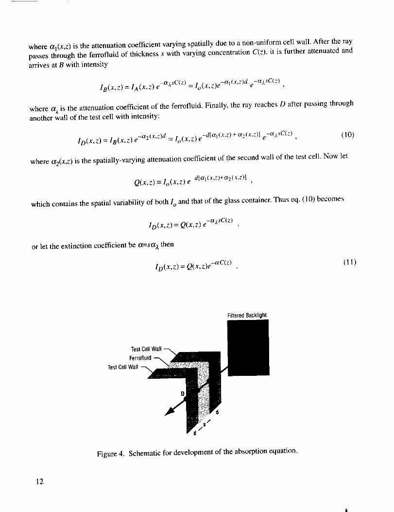
where tXl(X,Z) is the attenuation coefficient varying spatially due to a non-uniform cell wall. After the ray

passes through the ferrofluid of thickness s with varying concentration C(z), it is further attenuated and

arrives at B with intensity

IB(X, z) = IA (x, z) e -ct_'sC(z) = Io (x, z)e -al (x,z)d e-a;_sCt:) ,

where ct_ is the attenuation coefficient of the ferrofluid. Finally, the ray reaches D after passing through

another wall of the test cell with intensity:

ID(X, Z) = IB(X, z) e -a2 (x,z)d = io (x, z) e -dIal (x,z) + a 2(x,z)l e-a;yC(z) , ( I O)

where a2(x,z) is the spatially-varying attenuation coefficient of the second wall of the test cell. Now let

Q(x, z) =- Io(x, z) e -dIal (x'z)+a2(x'z)l ,

which contains the spatial variability of both Io and that of the glass container. Thus eq. (10) becomes

lo(x,z) = Q(x,z) e -a;_sC(z) ,

or let the extinction coefficient be t_=sa z then

ID(X, z) = Q(x, z)e -ac(z) (11)

FilteredBacklight

Test Cell Wall --_

Ferrofluid

Test Cell Wall

Figure 4. Schematic for development of the absorption equation.

12

To apply eq. ( 11 ) for retrieving the concentration, a vial of zero concentration (mineral oil only) was first

placed in front of the filtered backlight and the two-dimensional image of the cell was digitized. This array

is equivalent to Q(x,z) which is now known from eq. (11) using C=0. Next, a vial with a known, constant

fluid concentration C1,: was placed in front of the filtered backlight at the same location. This

two-dimensional image was digitized and stored as, say I_ (x,z). Then the extinction coefficient was

calculated from eq, (1 l) as

1 In Q(x,z)ct=_ lK(x,z ) (12)

Vf _

since everything on the right hand side is known. Averaging the fields Q(x,z) and I_(x, zJ before the

division or simply averaging the quotient yielded essentially the same value for a. Finally, the concentration

in any vial can now be determined by digitizing its image [ID(X,Z)] and computing the concentration from

eq. (I 1) as

C(z) = 1 In Q(x, z)a 1o(X,Z) (13)

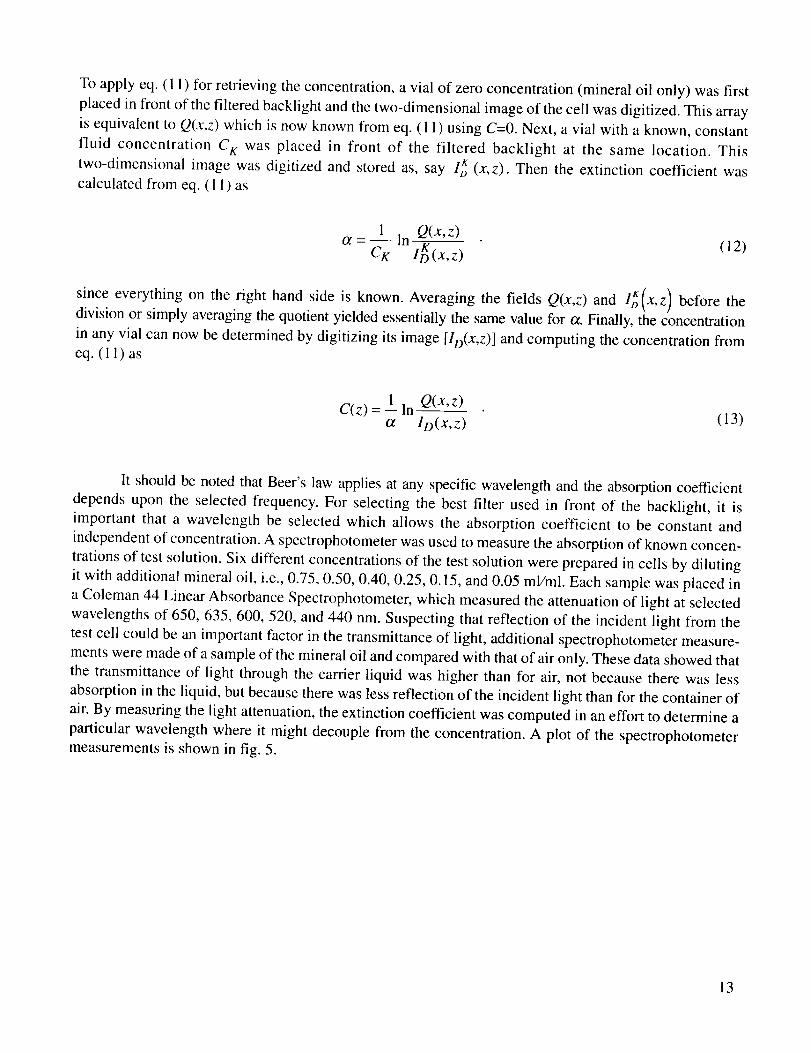
It should be noted that Beer's law applies at any specific wavelength and the absorption coefficient

depends upon the selected frequency. For selecting the best filter used in front of the backlight, it is

important that a wavelength be selected which allows the absorption coefficient to be constant and

independent of concentration. A spectrophotometer was used to measure the absorption of known concen-

trations of test solution. Six different concentrations of the test solution were prepared in cells by diluting

it with additional mineral oil, i.e., 0.75, 0.50, 0.40, 0.25, 0.15, and 0.05 mVml. Each sample was placed in

a Coleman 44 Linear Absorbance Spectrophotometer, which measured the attenuation of light at selected

wavelengths of 650, 635,600, 520, and 440 nm. Suspecting that reflection of the incident light from the

test cell could be an important factor in the transmittance of light, additional spectrophotometer measure-

ments were made of a sample of the mineral oil and compared with that of air only. These data showed that

the transmittance of light through the carrier liquid was higher than for air, not because there was less

absorption in the liquid, but because there was less reflection of the incident light than for the container of

air. By measuring the light attenuation, the extinction coefficient was computed in an effort to determine a

particular wavelength where it might decouple from the concentration. A plot of the spectrophotometer

measurements is shown in fig. 5.

13

A

30-25-

2O-TJ

= 15-0

10"0

5'

0

_ x x_

0.2 0.4 0.6 0.8

Concentration(ml/ml)

---4--- 650 nm

--0-- 635nm

---&--- 600 nm

520 nm

- _- 440 nm

Figure 5. The extinction coefficient versus concentration measured at

several wavelengths using a spectrophotometer.

It is clear that the extinction coefficient is fairly independent of concentration for the longer wave-

lengths so that red and green light would be candidates to use for photometrically measuring the concentra-

tion. From eq. (13), it can be seen that the relative error in concentration is proportional to the relative error

in the extinction coefficient

&C 6a-- ___-- °

C tx

Thus from fig. 5, the best extinction coefficient is the one that is independent of concentration with

the largest value (or) and the smallest variability (t_).

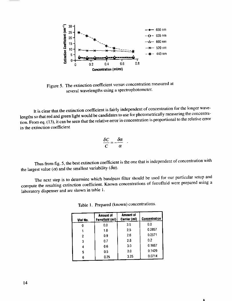
The next step is to determine which bandpass filter should be used for our particular setup and

compute the resulting extinction coefficient. Known concentrations of ferrofluid were prepared using a

laboratory dispenser and are shown in table 1.

Table 1. Prepared (known) concentrations.

Vial No.Amountof

Ferrofluid(ml)

0.0

1.0

0.9

0.7

0.6

0.5

0.25

Amountof

Carrier(ml)

3.5

2.5

2.6

2.8

3.0

3.0

3.25

Concentration

0.0

0.2857

0.2571

0.2

0.1667

0.1429

0.0714

14

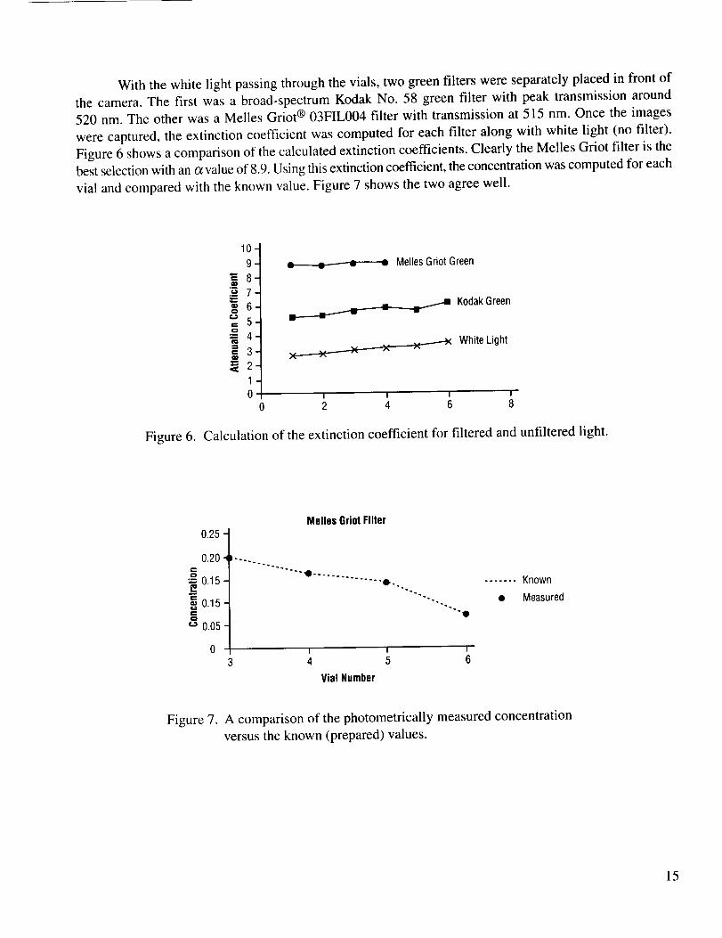
With the white light passing through the vials, two green filters were separately placed in front of

the camera. The first was a broad-spectrum Kodak No. 58 green filter with peak transmission around

520 nm. The other was a Melles Griot ® 03FIL004 filter with transmission at 515 nm. Once the images

were captured, the extinction coefficient was computed for each filter along with white light (no filter).

Figure 6 shows a comparison of the calculated extinction coefficients. Clearly the Melles Griot filter is the

best selection with an o_value of 8.9. Using this extinction coefficient, the concentration was computed for each

vial and compared with the known value. Figure 7 shows the two agree well.

Figure 6.

Q)

O

10

9

8

7

6

5

4

3

2

10

0

e,_ Melles Griot Green

_ Kodak Green

White Light

I I I I

2 4 6 8

Calculation of the extinction coefficient for filtered and unfiltered light.

0.25

0.20¢=o

= 0.15

_ 0.15O

0.05

Melles GriotFilter

......... o.. -...... Known

"'"'-. • Measured

I I I

3 4 5 6

Vial Number

Figure 7. A comparison of the photometrically measured concentration

versus the known (prepared) values.

15

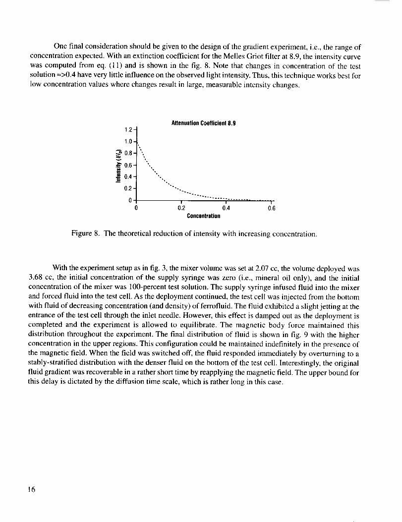
Onefinal considerationshouldbegivento thedesignof the gradient experiment, i.e., the range of

concentration expected. With an extinction coefficient for the Melles Griot filter at 8.9, the intensity curve

was computed from eq. (11) and is shown in the fig. 8. Note that changes in concentration of the test

solution =>0.4 have very little influence on the observed light intensity. Thus, this technique works best for

low concentration values where changes result in large, measurable intensity changes.

Figure 8.

1.2-

1.0-

O.8-

._ 0.6-IlJe-,

--.= 0.4_=

0.2

AttenuationCoefficient8.9

4

4

"'°''.° ...... . ...............

I I I

0.2 0.4 0.6

Concentration

The theoretical reduction of intensity with increasing concentration.

With the experiment setup as in fig. 3, the mixer volume was set at 2.07 cc, the volume deployed was

3.68 cc, the initial concentration of the supply syringe was zero (i.e., mineral oil only), and the initial

concentration of the mixer was 100-percent test solution. The supply syringe infused fluid into the mixer

and forced fluid into the test cell. As the deployment continued, the test cell was injected from the bottom

with fluid of decreasing concentration (and density) of ferrofluid. The fluid exhibited a slight jetting at the

entrance of the test cell through the inlet needle. However, this effect is damped out as the deployment is

completed and the experiment is allowed to equilibrate. The magnetic body force maintained this

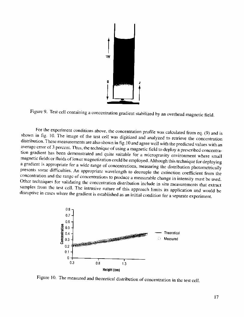
distribution throughout the experiment. The final distribution of fluid is shown in fig. 9 with the higher

concentration in the upper regions. This configuration could be maintained indefinitely in the presence of

the magnetic field. When the field was switched off, the fluid responded immediately by overturning to a

stably-stratified distribution with the denser fluid on the bottom of the test cell. Interestingly, the original

fluid gradient was recoverable in a rather short time by reapplying the magnetic field. The upper bound for

this delay is dictated by the diffusion time scale, which is rather long in this case.

16

T7//

g Z

ill

Figure 9. Test cell containing a concentration gradient stabilized by an overhead magnetic field.

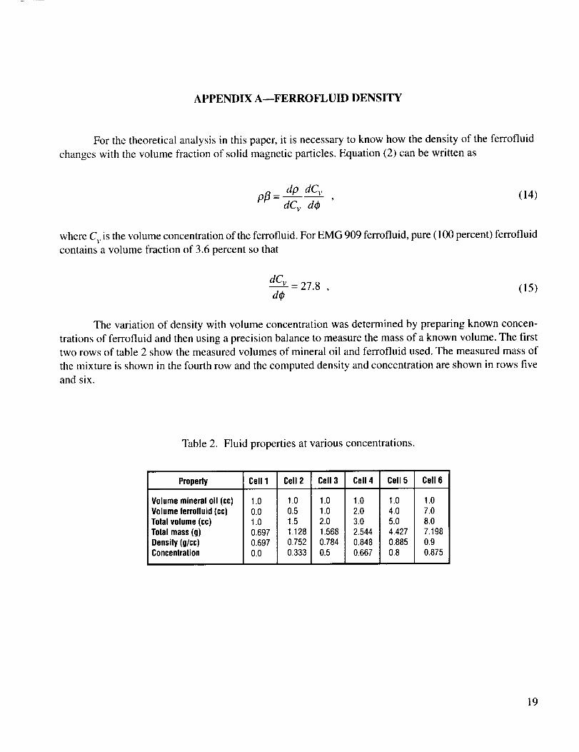
For the experiment conditions above, the concentration profile was calculated from eq. (9) and is

shown in fig. 10. The image of the test cell was digitized and analyzed to retrieve the concentration

distribution. These measurements are also shown in fig. 10 and agree well with the predicted values with an

average error of 3 percent. Thus, the technique of using a magnetic field to deploy a prescribed concentra-

tion gradient has been demonstrated and quite suitable for a microgravity environment where small

magnetic fields or fluids of lower magnetization could be employed. Although this technique for deploying

a gradient is appropriate for a wide range of concentrations, measuring the distribution photometrically

presents some difficulties. An appropriate wavelength to decouple the extinction coefficient from the

concentration and the range of concentrations to produce a measurable change in intensity must be used.

Other techniques for validating the concentration distribution include in situ measurements that extract

samples from the test cell. The intrusive nature of this approach limits its application and would be

disruptive in cases where the gradient is established as an initial condition for a separate experiment.

cgO

0.8

0.7

0.6

0.5

0.4

0.3

0.2

0.1

0| !

0,3 0.8 1,3

Height(cm)

u Theoretical

:_?:Measured

Figure 10. The measured and theoretical distribution of concentration in the test cell.

17

APPENDIX A--FERROFLUID DENSITY

For the theoretical analysis in this paper, it is necessary to know how the density of the ferrofluid

changes with the volume fraction of solid magnetic particles. Equation (2) can be written as

dp dC v (14)p[3- dCv ddp '

where C v is the volume concentration of the ferrofluid. For EMG 909 ferrofluid, pure (100 percent) ferrofluid

contains a volume fraction of 3.6 percent so that

dCv - 27.8 , (15)dO

The variation of density with volume concentration was determined by preparing known concen-

trations of ferrofluid and then using a precision balance to measure the mass of a known volume. The first

two rows of table 2 show the measured volumes of mineral oil and ferrofluid used. The measured mass of

the mixture is shown in the fourth row and the computed density and concentration are shown in rows five

and six.

Table 2. Fluid properties at various concentrations.

Property Cell1 Cell2 Cell3 Cell4 Cell5 Cell6

Volumemineraloil (cc) 1.0 1.0 1.0 1.0 1.0 1.0Volumeferrofluid(cc) 0.0 0.5 1.0 2.0 4.0 7.0Totalvolume(cc) 1.0 1.5 2.0 3.0 5.0 8.0Totalmass(g) 0.697 1.128 1.568 2.544 4.427 7.198Density(g/cc) 0.697 0.752 0.784 0.848 0.885 0.9Concentration 0.0 0.333 0.5 0.667 0.8 0.875

19

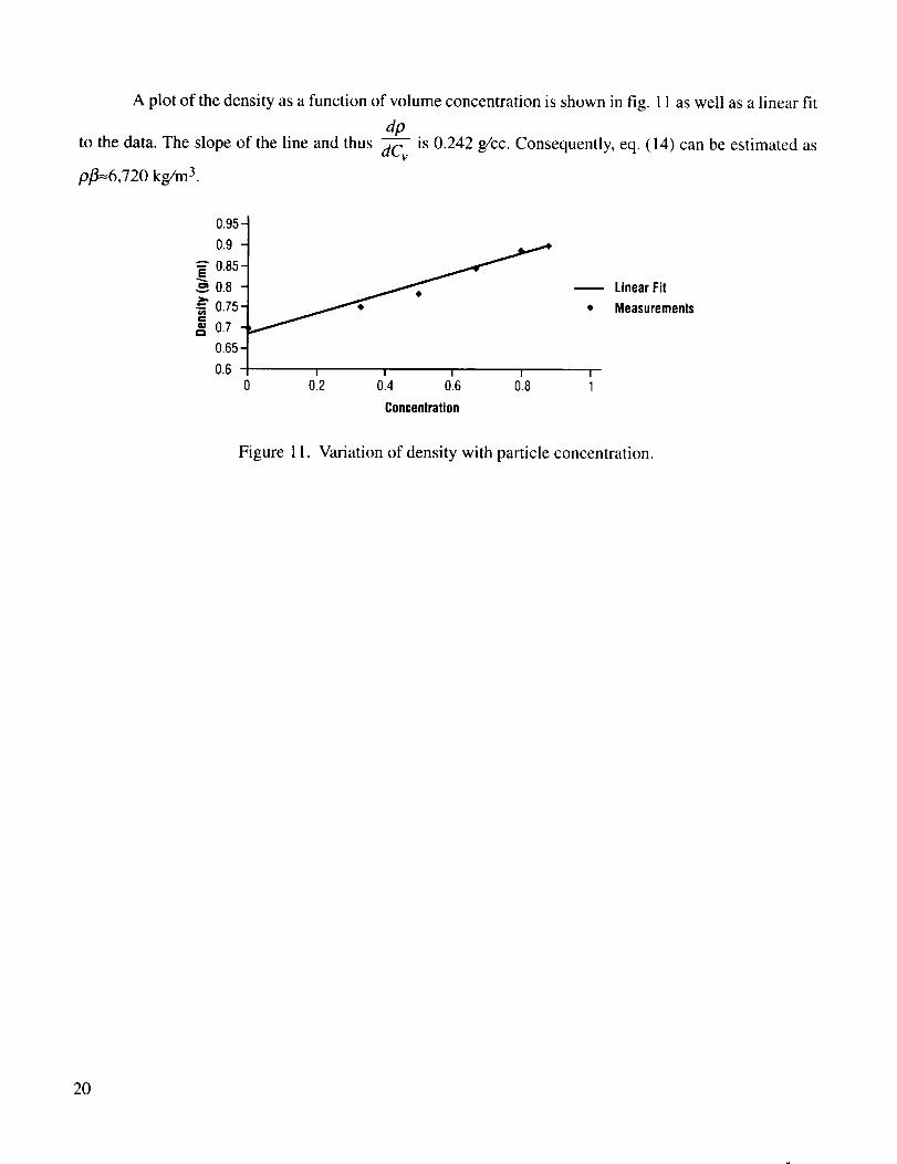
A plot of the density as a function of volume concentration is shown in fig. 11 as well as a linear fit

dr,to the data. The slope of the line and thus dC v is 0.242 g/cc. Consequently, eq. (14) can be estimated as

pj_-6,720 kg/m 3.

0.95-t

0°t_" 0.85=0.8-I

,-,0.7; "_0.65

O.6 I I I I I

0 0.2 0.4 0.6 0.8 1

Concentration

LinearFit

* Measurements

Figure 11. Variation of density with particle concentration.

20

APPENDIX BmCONCENTRATION GRADIENTS

B.1 General Case

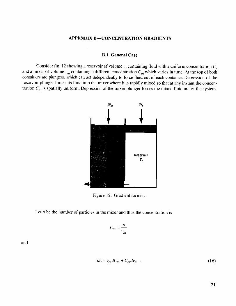
Consider fig. 12 showing a reservoir of volume V r containing fluid with a uniform concentration C r

and a mixer of volume vm containing a different concentration C m which varies in time. At the top of both

containers are plungers, which can act independently to force fluid out of each container. Depression of the

reservoir plunger forces its fluid into the mixer where it is rapidly mixed so that at any instant the concen-

tration C m is spatially uniform. Depression of the mixer plunger forces the mixed fluid out of the system.

dvm dvr

Figure 12. Gradient former.

Let n be the number of particles in the mixer and thus the concentration is

n

Cm=--Vm

and

dn = vmdC m + Cmdv m (16)

21

The number of particles flowing into the mixer from the reservoir is -CrdV r and the number of

particles flowing out of the mixer is -Cm(dvm+dvr). Thus, eq. (l 6) becomes

-Crdv r + Cm(dv m + dv r)= vmdC m + Cindy m

or

dvr = dCm (17)

v m (Cm-Cr)

Note that there is no change in the concentration of the mixer if either the volume of the reservoir is

constant, the mixer volume is very large, or if the concentration in the reservoir is the same as that in themixer.

B.2 Linear Gradient

If the two plungers are mechanically linked so that they move together, then dvr=dv m and eq. (17)becomes

dv m dC m

Vm (C m _Cr ) (18)

Integrating eq. (18) from the initial volume of the mixer Vmo at an initial concentration of Cmo to an

arbitrary volume and concentration gives

ff_o dvm = fCm dCm(C:-Cr)

or

Crn =C r +(Cmo-Cr) Vm (19)Vmo

The total volume deployed out of the mixer vt at any given time is 2(Vmo-Vm) so eq. (19) can also bewritten as

c,. =Cmo+(C,-Cmo)2 Vmo

(20)

22

B.3 Exponential Gradient

If the plunger of the mixer is fixed so that vm is a constant, then integrating the general eq. (17) from

an initial reservoir volume Vro when the mixer concentration is Cmo to an arbitrary volume and

concentration yields

f Cm dC ml _Vr'mo dvr= (Cm=-Cr)V171 Cmo

or

Cm =Cr+(Cmo-Cr)exp( vr-vr°)_,Vm (21)

The total volume deployed out of the mixer at any instant is Vro--V r to that eq. (21) can also bewritten as

Cm =Cr +(Cmo-Cr)eXp(-Vt ] .

_, VmJ(22)

The unit of concentration used here is particles per total volume. A more convenient measure is

volume concentration, which is the volume of test solution divided by the total volume of the mixture. This

volume concentration then is also equivalent to the above concentration divided by the number of particles

found in a unit volume of test solution. Since the two are related by a constant then both eq. (20) and eq. (22) arevalid for volume concentration as well.

23

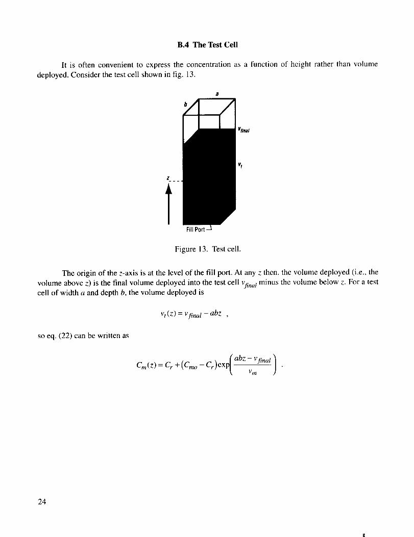
B.4 The Test Cell

It is often convenient to express the concentration as a function of height rather than volume

deployed. Consider the test cell shown in fig. 13.

a

b

I/final

TFill Port

Figure 13. Test cell.

The origin of the z-axis is at the level of the fill port. At any z then, the volume deployed (i.e., the

volume above z) is the final volume deployed into the test cell vfinal minus the volume below z. For a test

cell of width a and depth b, the volume deployed is

so eq. (22) can be written as

Vt(Z ) = Pfinal -- abz

l abz - Vfinal 1Cm(z)=C r +(Cmo-Cr)eXp --Vm

24

REFERENCES

1. Gillies, D.C.; Lehoczky, S.L.; Szofran, ER.; Watring, D.A.; Alexander, H.A.; and Jerman, G.A.:

"Directional Solidification of Mercury Cadmium Tellurium During the Second Microgravity Pay-

load Mission (USMP-2)," in Space Processing of Materials, N. Ramachandran (ed.),

SPIE 2809, pp. 2-11, 1996.

2. Odenbach, S.: "Convection Driven by Forced Diffusion in Magnetic Fluids," Phys. Fluids, Vol. 6,

pp. 2535-2539, 1994.

3. Neuringer, J.L.; and Rosensweig, R.E.: "Ferrohydrodynamics," Phys. Fluids, Vol. 7, no. 12,

p. 1927, 1964.

4. Zelazo, R.E.; and Melcher, J.R.: "Dynamics and Stability of Ferrofluids: Surface Interactions,"

J. Fluid Mech., Vol. 39, p. 1, 1969.

5. Finlayson, B.A.: "Convective Instability of Ferromagnetic Fluids," J. Fluid Mech., Vol. 40, p. 753,

1970.

6. Bashtovoi, V.G.; and Krakov, M.S.: "Stability of an Axisymmetric Jet of Magnetizable Fluid,"

translated from Z. Prik. Mekh. I Tekh. Fiz., No. 4, p. 147, July-August 1978.

7. Bashtovoi, V.G.: "Instability of a Motionless Thin Layer of a Magnetizable Liquid," translated from

Z. Prik. Mekh. I Tekh. Fiz., No. 1, p. 81, January-February 1978.

8. Bashtovoi, V.G.: "Convective and Surface Instability of Magnetic Fluids," Thermomechanics

of Magnetic Fluids, B. Berkovsky (ed.), Hemisphere Publishing Corporation, New York, NY,

pp. 159-179, 1978.

9. Schwab, L.; Hilderbrandt, U.; and Stierstadt, K.: "Magnetic Bdrnard Convection," J. Magnetism and

Magnetic Matls., Vol. 38, pp. 113-114, 1983.

10. Stiles, P.J.; and Kagan, M.: "Thermo-Convective Instability of a Horizontal Layer of Ferrofluid in a

Strong Vertical Magnetic Field," J. Magnetism and Magnetic Matls., Vol. 85, pp. 196-198, 1990.

11. Rosensweig, R.E.; Popplewell, J.; and Johnston, R.J.: "Magnetic Fluid Motion in a Rotating Field,"

J. Magnetism and Magnetic Matis., Vol. 85, p. 171, 1990.

12. Nakatsuka, K.; Hama, Y.; and Takahashi, J.: "Heat Transfer in Temperature-Sensitive Magnetic

Fluids," J. Magnetism and Magnetic Matls., Vol. 85, pp. 207-209, 1990.

25

13. Aihara, T.; Kim, J-K.; Okuyama, K.; and Lasek, A.: "Controllability of Convective Heat

Transfer of Magnetic Fluid in a Circular Tube," J. Magnetism and Magnetic Matls.,

Vol. 122, pp. 297-300, 1993.

14. Zebib, A.: "Thermal Convection in a Magnetic Fluid," J. Fluid Mech., Vol. 321, pp. 121-136, 1996.

15. Berkovsky, B.M.; and Smirnov, N.N.: "Capillary Hydrodynamic Effects in High Magnetic Fields,"

J. Fluid Mech., Vol. 187, p. 319, 1978.

16. H6rsten, W.V.; Odenbach, S.; and Stierstadt, K.: "Magnetic B6nard Convection Under Microgravity,"

Adv. Space Res., Vol. 11, pp. 251-254, 1991.

17. Odenbach, S.: "Drop Tower Experiments on Thermomagnetic Convection," Microgravity Sci. Technol.,

Vol. 6(3), pp. 161-163, 1993.

18. Odenbach, S.: "Sounding Rocket and Drop Tower Experiments on Thermomagnetic Convection in

Magnetic Fluids," Adv. Space Res., Vol. 16, pp. 99-104, 1995.

19. Rosensweig, R.E.: Ferrohydrodynamics, Cambridge University Press, NewYork, NY, 1985.

20. Turner, J.S.: Buoyancy Effect In Fluids, Cambridge University Press, New York, NY, 1973.

21. Mihailovic, J.; and Beckermann, C.: "Development of a Two-Dimensional Liquid Species

Concentration Measurement Technique Based on Absorptiometry," Exp. Thermal and Fluid Sci.;

Vol. 10, pp. 113-123, 1995.

26

Form ApprovedREPORT DOCUMENTATION PAGE OMBNo.0704-0188

Public reporting burden for this co#ection of information is estimated to average 1 hour per response, including the time for reviewing inslructions, searching existing data sources.gathering and maintaining the data needed, and completing and reviewing the collection of information Send comments regarding this burden estimate or any other aspect of thiscollection of information, including suggestions for reducing this burden, to Washington Headquarters Services, Directorate for Information Operation and Reports, 1215 JeffersonDavis Highway, Suite 1204, Arlington, VA 22202-4302, and to the Office ol Management and Budget, Paperwork Reduction ProleCl(0704-0188), Washington, DC 20503

1. AGENCY USE ONLY (Leave Blank) 2. REPORT DATE 3. REPORT TYPE AND DATES COVERED

July 2000 Technical Publication

4. TITLE AND SUBTITLE 5. FUNDING NUMBERS

The Use of Ferrofluids to Model Materials Processing(MSFC Center Director's Discretionary Fund Final Report, Project No. 98-12)

6. AUTHORS

F. Leslie and N. Ramachandran*

7. PERFORMINGORGANIZATIONNAMES(S)ANDADDRESS(ES)

George C. Marshall Space Flight Center

Marshall Space Flight Center, AL 35812

9, SPONSORING/MONITORINGAGENCYNAME(S)ANDADDRESS(ES)

National Aeronautics and Space Administration

Washington, DC 20546-0001

8. PERFORMING ORGANIZATION

REPORT NUMBER

M-985

10. SPONSORING/MONITORING

AGENCY REPORT NUMBER

NAS A/TP--2000-210386

11. SUPPLEMENTARY NOTES

Prepared by Microgravity Science and Applications Department, Science Directorate

*Universities Space Research Association, Huntsville, AL

12a. DISTRIBUTION/AVAILABILITY STATEMENT

Unclassified-Unlimited

Subject Category 34Nonstandard Distribution

12b. DISTRIBUTION CODE

13. ABSTRACT (Maximum 200 words)

Many crystals grown in space have structural flaws believed to result from convective motions during the growth

phase. The character of these instabilities is not well understood but is associated with thermal and solutal density

variations near the solidification interface in the presence of residual gravity and g-jitter. To study these instabilities

in a separate, controlled space experiment, a concentration gradient would first have to be artificially established in a

timely manner as an initial condition. This is generally difficult to accomplish in a microgravity environment because

the momentum of the fluid injected into a test cell tends to swirl around and mix in the absence of a restoring force.

The use of magnetic fields to control the motion and position of liquids has received recent, growing interest. The

possibility of using the force exerted by a non-uniform magnetic field on a ferrofluid to not only achieve fluid

manipulation but also to actively control fluid motion makes it an attractive candidate for space applications. This

paper describes a technique for quickly establishing a linear or exponential fluid concentration gradient using a

magnetic field in place of gravity to stabilize the deployment. Also discussed is a photometric technique for

measuring the concentration profile using light attenuation. Although any range of concentrations can be realized,

photometric constraints impose some limitations on measurements. Results of the ground-based experiments indicate

that the species distribution is within 3 percent of the predicted value.

14.SUBJECTTERMS

microgravity fluid dynamics, magnetic fluids

17. SECURITY CLASSIFICATION

OF REPORT

Unclassified

NSN7540-0i-280-SS00

18. SECURITY CLASSIFICATION

OF THIS PAGE

Unclassified

19. SECURITY CLASSIFICATION

OF ABSTRACT

Unclassified

15. NUMBER OF PAGES

3616. PRICE CODE

A0320. LIMITATION OF ABSTRACT

Unlimited

Standard Form 298 (Rev 2-89)PrescribeOby ANSI Std 239-18298-102