The use of dynamical networks to detect the hierarchical ...

Eur. Phys. J. B 73, 3–11 (2010) DOI: 10.1140/epjb/e2009-00286-0

The use of dynamical networks to detect the hierarchicalorganization of financial market sectors

T. Di Matteo, F. Pozzi and T. Aste

Eur. Phys. J. B 73, 3–11 (2010)DOI: 10.1140/epjb/e2009-00286-0

Regular Article

THE EUROPEANPHYSICAL JOURNAL B

The use of dynamical networks to detect the hierarchicalorganization of financial market sectors

T. Di Matteo1,2, F. Pozzi1, and T. Aste1,2,3,a

1 Applied Mathematics, Research School of Physical Sciences, The Australian National University, 0200 Canberra, Australia2 Department of Mathematics, King’s College, The Strand, London, WC2R 2LS, UK3 School of Physical Sciences, University of Kent, Canterbury, Kent CT2 7NH, UK

Received 27 February 2009 / Received in final form 22 May 2009Published online 18 August 2009 – c© EDP Sciences, Societa Italiana di Fisica, Springer-Verlag 2009

Abstract. Two kinds of filtered networks: minimum spanning trees (MSTs) and planar maximally filteredgraphs (PMFGs) are constructed from dynamical correlations computed over a moving window. We studythe evolution over time of both hierarchical and topological properties of these graphs in relation tomarket fluctuations. We verify that the dynamical PMFG preserves the same hierarchical structure as thedynamical MST, providing in addition a more significant and richer structure, a stronger robustness anddynamical stability. Central and peripheral stocks are differentiated by using a combination of differenttopological measures. We find stocks well connected and central; stocks well connected but peripheral;stocks poorly connected but central; stocks poorly connected and peripheral. It results that the Financialsector plays a central role in the entire system. The robustness, stability and persistence of these findingsare verified by changing the time window and by performing the computations on different time periods.We discuss these results and the economic meaning of this hierarchical positioning.

PACS. 89.65.Gh Economics; econophysics, financial markets, business and management – 89.75.FbStructures and organization in complex systems – 95.75.Wx Time series analysis, time variability

1 Introduction

In the last few years different methods have been proposedfor filtering relevant information in financial data by ex-tracting a structure of interactions from cross-correlationmatrices where only a subset of relevant entries are se-lected by means of criteria borrowed from network the-ory [1–14]. In particular, two methods that have beenproved to be very effective are the Minimum SpanningTree (MST ) [1,15] and the Planar Maximally FilteredGraph (PMFG) [7,8]. Both methods are based on an it-erative construction of a constrained graph (a tree or aplanar [16] graph) which retains the largest correlationsbetween connected nodes.

In this paper we analyze daily time series of then = 300 most capitalized NY SE stocks from 2001 to2003, for a total of T = 748 days [9]. Return time se-ries are computed as logarithmic differences of daily pricesYs(t) = log (Ps(t + 1)) − log (Ps(t)) (s = 1...300), anddaily prices are computed as averages of daily quotations.Closing quotations are excluded from the computation.Stocks are classified into 12 economic sectors and 77 eco-nomic subsectors, according to the classification of Forbesmagazine. Names of sectors, the labels used in this paperand the number of stocks in each sector are reported inTable 1.

a e-mail: [email protected]

We have considered moving windows from time (t) totime (t + ∆t − 1), where t = 1, 2 , ..., T − ∆t + 1 and∆t = 21, 42, 63, 84, 126, 251 market days, correspond-ing approximately to ∆t = 1, 2, 3, 4, 6, 12 months.

For each of the resulting time series Ys(t), we have com-puted the correlation matrix C (t, ∆t) whose coefficientsare given by the following formula:

ci,j (t, ∆t) =〈YiYj〉(t,∆t) − 〈Yi〉(t,∆t) 〈Yj〉(t,∆t)√(⟨

Y2

i

⟩(t,∆t)

− 〈Yi〉2(t,∆t)

) (⟨Y

2

j

⟩(t,∆t)

− 〈Yj〉2(t,∆t)

) ,

(1)

where 〈f〉(t,∆t) = 1∆t

∆t−1∑τ=0

f(t + τ) is the time average of

a given time series f(τ) over the window ∆t from timet to time t + ∆t − 1. From these correlation coefficientsci,j , we compute distances between stocks i and j: di,j =√

2 (1 − ci,j) [1,17–19]. The resulting matrix D (t, ∆t) =√2 (1 − C (t, ∆t)) is the dynamical distance matrix of the

weighted complete graph which has n(n− 1)/2 edges con-necting all pairs of nodes. Different methods exist in liter-ature in order to filter the information contained in sucha huge amount of data, otherwise hardly readable andusable.

4 The European Physical Journal B

Table 1. Name of sectors, Labels and corresponding Numberof Stocks.

Sector Label Number of StocksBasic Materials S01 24Capital Good S02 12Conglomerates S03 8

Consumer Cyclical S04 22Consumer Non Cyclical S05 25

Energy S06 17Financial S07 53Healthcare S08 19Services S09 69

Technology S10 34Transportation S11 5

Utilities S12 12

In this paper we filter this information by using mini-mal graphs, namely MST (a connected graph with no cy-cles and n−1 edges, [20]) and PMFG (a connected planargraph [16] in which the number of edges is 3n− 6 [8,21]).Such graphs are generated dynamically from correlationscomputed over a moving window. Dynamics adds a quan-tification of stability/variability over time which is veryimportant in systems such as financial markets that areconstantly evolving. In previous papers [8,21], it has beenproved that the MST is always a subgraph of the PMFGand the dynamical PMFG preserves the same hierarchicalstructure as the dynamical MST , providing also a moresignificant and richer structure, a stronger robustness anda better dynamical stability. In this paper we investigatethe hierarchical positioning of stocks in MST and PMFGgraphs by computing the Degree, Betweenness, Eccentric-ity and Closeness and we obtain a clear differentiation ofstocks in terms of centrality and peripherality.

In Section 2 we report the results concerning the De-gree, Betweenness, Eccentricity and Closeness of MSTand PMFG graphs; we also discuss the changes in thegraph organization with respect to the window size ∆t.In Section 3 a principal component analysis and a clus-ter analysis are performed. The stability over time of theresults is also analyzed. Conclusions are given in Section 4.

2 Centrality and peripherality measures

Our aim in this work is to classify each stock in termsof its relative position in the network by quantitativelydistinguishing between nodes that are more or less cen-tral. To this aim, for each node of both dynamical MST sand PMFGs and for each ∆t we have computed the timeaverage of Degree, Betweenness, Eccentricity and Close-ness [22,23], which are defined as follows1:

– the Degree of a node is the number of edges connectedto that node;

– the Betweenness of node i is the total number of short-est paths between all possible pairs of vertices that

1 We consider unweighted, undirected connected graphs only.

pass through node i. The Shortest Path (or geodesic)between node k and node j is the shortest chain of con-nected pairs of vertices joining vertices k and j. Thelength of a path from node k to node j is the numberof edges included in the path;

– the Eccentricity of node i is the maximum length ofthe shortest paths that connect i to any other node j;

– the Closeness of node i is the average length of allShortest Paths that connect i and any other node j.

It is clear from the definition that Degree and Betweennessare ‘centrality’ measures which return larger valuesfor more central, better connected, nodes; converselyEccentricity and Closeness are ‘peripherality’ measures re-turning larger values for less central nodes.

In order to assess the relevance of sectors from a cen-trality/peripherality point of view we made several rank-ings of the stocks sorted respectively in descending orderfor Degree and Betweenness and ascending order for Ec-centricity and Closeness. For each sector we then countedthe number of stocks present in the top fifty positions andin the bottom fifty positions of the rankings. Results arereported in Table 2 for ∆t = 1 and 12.

We find that the Financial sector (S07) is alwaysstrongly predominant among the central nodes of the sys-tem. This predominant role is retrieved in all the fourmeasures, for all ∆t, both for the dynamical MST s andPMFGs. Such predominance slightly decreases as ∆t in-creases. Though proportions are very similar for all thefour measures, Eccentricity and Closeness show higher fig-ures than Degree and Betweenness. Other strong presencesamong the central nodes can also be attributed to Ba-sic Materials (S01), Capital Goods (S02), Conglomerates(S03), Consumer Cyclical (S04). We note, in particular,that the sector Basic Materials appears very central when∆t = 1 month but its centrality gradually fades awaywhen ∆t increases. Technology (S10) and Services (S09)have a more mixed positioning, indeed they occupy manyof the lower fifty most peripheral positions, according tothe Degree and the Betweenness but they do not have highEccentricity and Closeness. Conversely, very high relativevalues of Eccentricity and Closeness are found in nodesbelonging to Utilities (S12), Energy (S06), Consumer NonCyclical (S05). In particular, we find absolutely outstand-ing the relevance of Utilities sector where most of the 12Utilities stocks are counted among the fifty stocks withlargest Eccentricity and largest Closeness. Other sectors,such as Healthcare (S08) and Transportation (S11) ranklow in all the measures resulting therefore nor central nei-ther peripheral. We find particularly noteworthy the sim-ilarity in behaviors of MST s and PMFGs which show aremarkable correspondence of sectorial structures.

2.1 Effect of the time-window

From Table 2 it emerges that changes in the ranking oc-cur as the time window ∆t changes. In order to checkand quantify the robustness of these results with re-spect to ∆t, we have computed for all measures the av-erage over time t at different ∆t values for each stock.

T. Di Matteo et al.: Hierarchical organization of financial market sectors 5

Table 2. Number of stocks, for each sector, among the fifty top and the fifty bottom values for Degree, Betweenness, Eccentricityand Closeness for both MST and PMFG, for ∆t = 1 and 12. In boldface are highlighted the most central or peripheral sectorsaccordingly with each measure.

Degree (descending order)

(a) MST ’s Top Fifty (a) (b) PMFG’s Top Fifty (b)

S01 S02 S03 S04 S05 S06 S07 S08 S09 S10 S11 S12 S01 S02 S03 S04 S05 S06 S07 S08 S09 S10 S11 S12

∆t = 1 8 3 2 3 1 1 25 0 2 5 0 0 8 3 3 3 1 2 26 0 1 3 0 0

∆t = 12 3 3 3 2 5 4 15 2 8 3 0 2 4 3 3 2 5 2 17 2 5 6 0 1

(c) MST ’s Bottom Fifty (c) (d) PMFG’s Bottom Fifty (d)


∆t = 1 3 1 0 1 9 2 3 7 14 9 0 1 3 2 0 1 8 2 2 7 15 7 1 2

∆t = 12 3 0 1 2 7 1 4 2 14 14 0 2 4 0 0 3 5 2 3 2 14 15 1 1

Betweenness (descending order)

(e) MST ’s Top Fifty (e) (f) PMFG’s Top Fifty (f)


∆t = 1 10 3 3 2 0 1 27 0 0 4 0 0 8 3 4 2 0 2 27 0 1 3 0 0

∆t = 12 3 3 3 5 2 5 17 2 7 3 0 0 4 3 3 4 2 5 18 2 5 4 0 0

(g) MST ’s Bottom Fifty (g) (h) PMFG’s Bottom Fifty (h)


∆t = 1 2 1 0 1 10 2 4 8 17 4 1 0 2 1 0 1 9 2 7 7 16 5 0 0

∆t = 12 4 1 1 2 7 1 5 2 11 15 0 1 2 0 0 2 6 3 6 2 15 13 1 0

Eccentricity (ascending order)

(i) MST ’s Top Fifty (i) (l) PMFG’s Top Fifty (l)


∆t = 1 11 4 4 3 0 0 28 0 0 0 0 0 11 3 4 2 0 0 29 0 0 1 0 0

∆t = 12 2 3 4 4 0 1 22 0 8 6 0 0 1 3 2 3 0 2 21 0 14 4 0 0

(m) MST ’s Bottom Fifty (m) (n) PMFG’s Bottom Fifty (n)


∆t = 1 2 0 0 0 7 13 2 6 7 1 0 12 2 0 0 0 12 11 1 5 7 1 0 11

∆t = 12 4 1 0 1 14 10 0 2 8 1 0 9 5 3 0 2 13 10 0 2 6 1 0 8

Closeness (ascending order)

(o) MST ’s Top Fifty (o) (p) PMFG’s Top Fifty (p)


∆t = 1 10 3 4 4 0 0 29 0 0 0 0 0 9 3 5 3 0 0 29 0 0 1 0 0

∆t = 12 3 3 6 7 0 0 23 0 5 3 0 0 2 3 4 6 0 1 20 1 10 3 0 0

(q) MST ’s Bottom Fifty (q) (r) PMFG’s Bottom Fifty (r)


∆t = 1 2 0 0 0 8 13 2 6 6 1 0 12 2 1 0 0 9 12 1 5 7 1 0 12

∆t = 12 3 1 0 1 10 14 1 2 7 1 0 10 4 1 0 1 11 12 0 2 6 2 0 11


Fig. 1. (Color online) (Above) Average Degree as functionof ∆t for the stocks having the highest relative Degree withintheir own sector. (Below) Average Degree as function of ∆t forthe stocks having the lowest relative Degree within their ownsector.

In particular, we have computed how the average Degreein the PMFG for each of the 300 stocks changes when ∆tincreases. We found a decrease for 67% of stocks and anincrease for the remaining 33%. Since the average Degreefor a PMFG is a constant, the sum of negative and pos-itive values must be zero. Therefore, there are only fewstocks in the graph which become more central but thosestocks acquire in proportion a larger number of links. Weobserve a similar behavior for the Betweenness. On theother hand, Closeness and Eccentricity reveal a differentbehavior showing a clear decreasing trend in the lowestvalues but rather stationary or even decreasing trends forthe highest values. This is due to the fact that the overallaverage for both measures is decreasing with ∆t.

In order to better visualize such different behaviors inFigures 1–4 we report respectively the average Degree,average Betweenness, average Eccentricity and averageCloseness as function of ∆t for a selection of stocks havingrespectively the highest relative values and lowest relativevalues. The data refer to PMFG graphs only but MSTshave very similar properties and trends. We observe that

Fig. 2. (Color online) (Above) Average Betweenness as func-tion of ∆t for the stocks having the highest relative Degreewithin their own sector. (Below) Average Betweenness as func-tion of ∆t for the stocks having the lowest relative Degreewithin their own sector.

–as a general trend– the differentiation between centraland peripheral nodes in terms of Degree and Betweennessbecomes stronger with increasing trends for high valuesand decreasing trends for low values. This is a indicationthat the graphs become increasingly structured when thewindow-size increases.

Let us note that most of the stocks reported in Figure 1are also present in Figure 2 and most of the stocks reportedin Figure 3 are also in Figure 4.

3 Principal component analysis and clusteranalysis

The analysis of Degree, Betweenness, Eccentricity andCloseness introduced in the previous section, suggests thatthere could be two different gatherings of the variableswhich fully explain the different classifications obtainedfrom Degree and Betweenness on one side and Eccen-tricity and Closeness on the other. In order to increaserobustness, we have calculated all the quantities for all


Fig. 3. (Color online) (Above) Average Eccentricity as func-tion of ∆t for the stocks having the highest relative Degreewithin their own sector. (Below) Average Eccentricity as func-tion of ∆t for the stocks having the lowest relative Degreewithin their own sector.

Dynamical MSTs and for all Dynamical PMFGs, for alltime periods and all the running windows. In order tocompare all these different measures we have transformedthem in Fractional Rankings2. Then, for each measure, foreach running window and for each stock, for both MSTsand PMFGs, we compute the time average of rankings.Afterwards, for each measure, for each stock and for bothMSTs and PMFGs, we compute the average with respectto the running windows. This average ranking procedureprovides four synthetic measures for Degree, Betweenness,(–)Eccentricity and (–)Closeness and for both MST andPMFG (eight variables in total).

Principal Components analysis of these 8 variablesyields to two significant principal factors. The first prin-cipal factor is essentially an average of all the eightvariables and it explains the 74% of the total variancewith 82–88% correlation between all the measures. Nodesthat are highly connected and in central positions inthe network have high relative scores for this measure.

2 In Fractional Ranking, the same mean rank is assigned toentries with the same score.

Fig. 4. (Color online) (Above) Average Closeness as functionof ∆t for the stocks having the highest relative Degree withintheir own sector. (Below) Average Closeness as function of ∆tfor the stocks having the lowest relative Degree within theirown sector.

The second principal factor is also statistically significant,explaining 24% of the total variance and it is essentiallythe sum of the first two measures (Degree, Betweenness)minus the second two ((–)Eccentricity and (–)Closeness).This component gives high scores to nodes that are highlyconnected but that do not reside in central regions of thenetwork.

Let us here report some stocks selected in terms of thetwo principal components:

1) nodes with the largest values of the first component(highly connected and central): A.G. Edwards (AGE),Franklin Resources (BEN) and Merrill Lynch (MER)belonging to the Financial sector (S07);

2) nodes with the largest values of the second compo-nent (highly connected but eccentric): Eastman Kodak(EK), Leucadia National (LUK), Golden West Finan-cial (GDW) and Unisys (UIS);

3) nodes with the smallest values of the first compo-nent (poorly connected and peripheral): Health CareProperty Invs (HCP), Valero Energy (VLO), Sara Lee(SLE) and Sociedad Anonima ADS (YPF);


Fig. 5. (Color online) Stocks belonging to two different sectorsare clearly differentiated in terms of their positions within thenetwork: the energy sector (large squares, figure above) is inthe periphery of the graphs whereas the financial sector (largestars, figure below) resides mostly in the central regions of thegraphs.

4) nodes with the smallest values of the second compo-nent (non peripheral but poorly connected): Apache(APA), Kerr-Mcgee (KMG), Colgate-Palmolive (CL)and Smith International (SII);

5) nodes neutral from both points of view (nor partic-ularly well connected and neither especially central):Best Buy (BBY), Jones Apparel (JNY) and Meredith(MDP).

Within this classification we can recognize regions domi-nated by particular sectors. For instance, in Figure 5 wecan see that stocks belonging to the Energy sector are allclearly placed in the region of large Eccentricity whereasstocks belonging to the Financial sector stay mostly in theregion of high connectivity and high centrality. We notehowever that in Figure 5 there are two stocks belonging tothe Financial sector that appear to stay in rather eccentricregions, separated from the other Financial stocks. A care-ful scrutiny reveals that these stocks are belonging to the

sub-sector “Insurance accidental & health”. Interestingly,the region where they are confined is highly populated bystocks belonging to Healthcare.

3.1 Cluster analysis

In order to better differentiate the relative positioning ofthe stocks and their gathering in central or peripheral re-gions, we have performed a cluster analysis [18,24] usingthe 8 synthetic measures from Fractional Rankings de-scribed in the previous section. This leads to the followingsix clusters which are enclosed inside the polyhedral linesin Figure 5. The analysis has been performed by usingSPAD software where a hierarchical tree (dendrogram) hasbeen constructed based on all the axes obtained by Princi-pal Components analysis and Wards aggregation criterionwith a cut performed using a consolidation procedure [24].We verified that the qualitative gathering of the stocks isrobust and independent on the details of the clusteringprocedure with exception for some stocks at the clusterboundaries which might be swapped between neighboringclusters.

In one cluster we find 44 stocks that are both extremelycentral and well connected. This cluster contains BEN andMER, it is dominated by 25 financial stocks, with a muchlighter presence of stocks belonging to Basic Materials (6),Conglomerates (4) and Capital Good (3).

In a second cluster we find 66 stocks that are cen-tral and connected, but less than the first cluster andwith some stocks that tend to be slightly eccentric incertain occasions but still remain well connected. Thereare again many stocks belonging to the Financial sector(10). Significant are also the stocks belonging to ConsumerCyclical (12), Basic Materials (7), Conglomerates (2) andCapital Good (4). There are also 15 stocks from Servicesand 7 from Technology.

A third cluster is characterized by 45 stocks that areeccentric but well connected. This cluster contains APA(Apache corp, S06) and it is dominated by Utilities (9),Energy (12), Consumer Non Cyclical (10), with a moder-ate presence of Services as well (8).

Scarcely connected but neither eccentric are the 53stocks belonging to a fourth cluster. This cluster containsLUK (Leucadia National Corp, S03) and it is mainly com-posed by stocks belonging to Technology (13), Services(19), and Financial (10) sectors.

A fifth cluster is characterized by 51 stocks which arepoorly connected and peripheral and it isn’t clearly char-acterized from a sectorial point of view, apart from 14stocks belonging to Services.

In a sixth cluster we find 41 stocks that are alwaysperipheral and poorly connected. There are 10 stocks ofConsumer Non Cyclical, 8 from Healthcare and 9 fromServices. This cluster contains SLE (Sara Lee corp, S05).

3.2 Persistence over time

It is now quite clear that the above measures can distin-guish well between stocks in central or peripheral positions


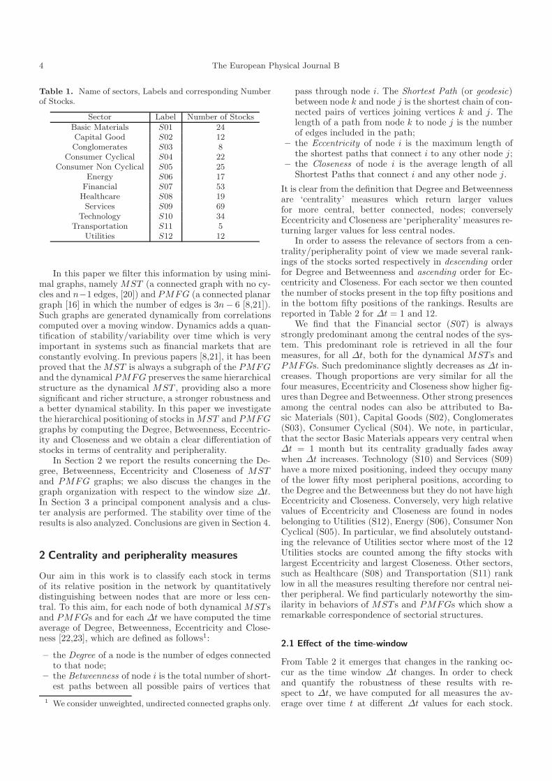
Fig. 6. (Color online) Average rankings ordered by De-gree, Betweenness, (–)Eccentricity and (–)Closeness, for ∆t =12 months as function of time. Data are for BEN (S07),LUK(S03), APA (S06) and SLE (S05).

in the network and that this differentiation is consistentwith the independent classification of the stocks accord-ingly to their economic sector. We now want to verifyif such classification is persistent with time. To this endwe follow the measure associated with the x-axis in Fig-ure 5 over time for four stocks belonging to the first,fourth, third and sixth cluster, namely BEN (S07), LUK(S03), APA (S06) and SLE (S05). Accordingly to the pre-vious analysis BEN and SLE are respectively very centraland very peripheral, whereas APA and LUK have a moremixed location. Indeed, in Figure 6 we observe that LUKand APA are fluctuating around the mean value (150)while BEN is well above and SLE is well below the average.

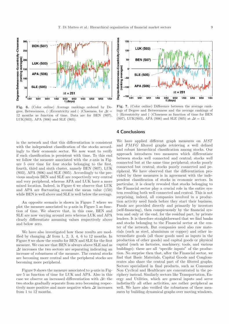
An opposite scenario is shown in Figure 7 where weplot the measure associated to y-axis in Figure 5 as func-tion of time. We observe that, in this case, BEN andSLE are now varying around zero whereas LUK and APAclearly differentiate assuming values respectively aboveand below zero.

We have also investigated how these results are mod-ified by changing ∆t from 1, 2, 3, 4, 6 to 12 months. InFigure 8 we show the results for BEN and SLE for the firstmeasure. We can see that BEN is always above SLE and as∆t increases the two sectors are separating indicating anincrease of robustness of the measure. The central stocksare becoming more central and the peripheral stocks arebecoming more peripheral.

Figure 9 shows the measure associated to y-axis in Fig-ure 5 as function of time for LUK and APA. Also in thiscase we observe an increased differentiation with ∆t: thetwo stocks gradually separate from zero becoming respec-tively more positive and more negative when ∆t increasesfrom 1 to 12 months.

Fig. 7. (Color online) Difference between the average rank-ings of Degree and Betweenness and the average rankings of(–)Eccentricity and (–)Closeness as function of time for BEN(S07), LUK(S03), APA (S06) and SLE (S05) at ∆t = 12.

4 Conclusions

We have applied different graph measures on MSTand PMFG filtered graphs retrieving a well definedand robust hierarchical classification among stocks. Ourapproach introduces two measures which differentiatebetween stocks well connected and central; stocks wellconnected but at the same time peripheral; stocks poorlyconnected but central; stocks poorly connected and pe-ripheral. We have observed that the differentiation pro-vided by these measures is in agreement with the inde-pendent classification of stocks in economic sectors. Inparticular, it is clearly revealed that stocks belonging tothe Financial sector play a crucial role in the entire sys-tem resulting both well connected and central. This is notsurprising, indeed, all companies involved in a produc-tion activity need funds before they start their business.Funds are provided directly and primarily by investors(self-financing), then conspicuously by the financial sys-tem and only at the end, for the residual part, by privatelenders. It is therefore straightforward that we find banksand stocks belonging to the Financial sector at the cen-ter of the network. But companies need also raw mate-rials (such as steel, aluminium or copper) and other in-termediate goods (all those goods used as inputs in theproduction of other goods) and capital goods or physicalcapital (such as factories, machinery, tools, and variousbuildings): these are all “specific inputs” of the produc-tion. No surprise then that, after the Financial sector, wefind that Basic Materials, Capital Goods and Conglom-erates also share the central part of the filtered graphs.Sectors specialized in final products, such as ConsumerNon Cyclical and Healthcare are concentrated in the pe-riphery instead. Similarly sectors like Transportation, En-ergy and Utilities, which are general inputs and serveindistinctly all other activities, are rather peripheral aswell. We have also verified the robustness of these mea-sures by building dynamical graphs over moving windows.


Fig. 8. (Color online) Average rankings ordered by Degree, Betweenness, (–)Eccentricity and (–)Closeness as function of timefor BEN (S07) and SLE (S05) for ∆t = 1 month (a), 2 months (b), 3 months (c), 4 months (d), 6 months (e) and 12 months(f).

Fig. 9. (Color online) Difference between the average of Degree and Betweenness rankings and the average of (–)Eccentricityand (–)Closeness rankings as function of time for APA (S06) and LUK(S03) for ∆t = 1 month (a), 2 months (b), 3 months (c),4 months (d), 6 months (e) and 12 months (f).


The results show that this classification is robust over timeand the differentiation becomes stronger when the windowsize increases. The dynamical changes in such hierarchi-cal structuring associated with market turbulences, willbe the topic of future studies.

This work was partially supported by the ARC DiscoveryProjects DP0344004 (2003), DP0558183 (2005) and COSTMP0801 project.

References

1. R.N. Mantegna, EPJB 11, 193 (1999)2. S.H. Strogatz, Nature 410, 268 (2001)3. J.-P. Onnela, M.Sc. Thesis, Department of Electrical

and Communications Engineering, Helsinki University ofTechnology (2002)

4. J.-P. Onnela, A. Chakraborti, K. Kaski, J. Kertesz, EPJB30, 285 (2002)

5. J.-P. Onnela, A. Chakraborti, K. Kaski, J. Kertesz, A.Kanto, Phys. Rev. E 68, 056110 (2003)

6. J.-P. Onnela, A. Chakraborti, K. Kaski, J. Kertesz,Physica A 324, 247 (2003)

7. T. Aste, T. Di Matteo, S.T. Hyde, Physica A 346, 20(2005)

8. M. Tumminello, T. Aste, T. Di Matteo, R.N. Mantegna,PNAS 102/30, 10421 (2005)

9. M. Tumminello, T. Aste, T. Di Matteo, R.N. Mantegna,EPJB 55, 209 (2007)

10. H.M. Ohlenbusch, T. Aste, B. Dubertret, N. Rivier, EPJB2, 211 (1998)

11. T. Aste, D. Sherrington, J. Phys. A 32, 7049 (1999)12. T. Aste, T. Di Matteo, M. Tumminello, R.N. Mantegna,

Proc. SPIE 5848, 100 (2005)13. T. Aste, T. Di Matteo, Physica 370, 156 (2006)14. T. Di Matteo, T. Aste, Proc. SPIE 6039, 60390P-1 (2006)15. J.C. Gower, G.J.S. Ross, Applied Statistics 18/1, 54

(1969)16. A planar graph is a graph that can be represented on an

Euclidean plane with no intersections between edges17. T. Di Matteo, T. Aste, International Journal of Theoretical

and Applied Finance 5/1, 107 (2002)18. T. Di Matteo, T. Aste, R.N. Mantegna, Physica A 339,

181 (2004)19. T. Di Matteo, T. Aste, S.T. Hyde, S. Ramsden, Physica A

355, 21 (2005)20. J. Eisner, Manuscript, University of Pennsylvania (1997)21. F. Pozzi, T. Aste, G. Rotundo, T. Di Matteo, Proc. SPIE

6802, 68021E (2008)22. G. Caldarelli, Scale-Free Networks. Complex Webs in

Nature and Technology (Oxford University Press, 2007)23. S.N. Dorogovtsev, J.F.F. Mendes, Evolution of Networks.

From Biological Nets to the Internet and WWW (OxfordUniversity Press, 2003)

24. L. Lebart, A. Morineau, M. Piron, Statistique exploratoiremultidimensionnelle (Dunod, Paris, 1995), Chap. 2,pp. 155–175

The use of dynamical networks to detect the hierarchical ...

Documents

Transcript of The use of dynamical networks to detect the hierarchical ...