THE USE OF A TRI-AXIAL ACCELEROMETER TO MEASURE …

Virginia Commonwealth University Virginia Commonwealth University

VCU Scholars Compass VCU Scholars Compass

Theses and Dissertations Graduate School

2009

THE USE OF A TRI-AXIAL ACCELEROMETER TO MEASURE THE USE OF A TRI-AXIAL ACCELEROMETER TO MEASURE

CHANGES IN LOWER EXTREMITY FATIGUE DURING FUNCTIONAL CHANGES IN LOWER EXTREMITY FATIGUE DURING FUNCTIONAL

ACTIVITY ACTIVITY

Kristin Morgan Virginia Commonwealth University

Follow this and additional works at: https://scholarscompass.vcu.edu/etd

Part of the Biomedical Engineering and Bioengineering Commons

© The Author

Downloaded from Downloaded from https://scholarscompass.vcu.edu/etd/1924

This Thesis is brought to you for free and open access by the Graduate School at VCU Scholars Compass. It has been accepted for inclusion in Theses and Dissertations by an authorized administrator of VCU Scholars Compass. For more information, please contact [email protected].

http://www.vcu.edu/

http://www.vcu.edu/

https://scholarscompass.vcu.edu/

https://scholarscompass.vcu.edu/etd

https://scholarscompass.vcu.edu/gradschool

https://scholarscompass.vcu.edu/etd?utm_source=scholarscompass.vcu.edu%2Fetd%2F1924&utm_medium=PDF&utm_campaign=PDFCoverPages

http://network.bepress.com/hgg/discipline/229?utm_source=scholarscompass.vcu.edu%2Fetd%2F1924&utm_medium=PDF&utm_campaign=PDFCoverPages

https://scholarscompass.vcu.edu/etd/1924?utm_source=scholarscompass.vcu.edu%2Fetd%2F1924&utm_medium=PDF&utm_campaign=PDFCoverPages

mailto:[email protected]

THE USE OF A TRI-AXIAL ACCELEROMETER TO MEASURE CHANGES IN

LOWER EXTREMITY FATIGUE DURING FUNCTIONAL ACTIVITY

A thesis submitted in partial fulfillment of the requirements for the degree of Master of

Science at Virginia Commonwealth University

By

Kristin Denise Morgan

Bachelor of Science, Duke University, 2007

Director: Peter Pidcoe, Ph.D., P.T., Assistant Professor, Department of Physical Therapy

Co-Director: Gerald Miller, Ph.D., Chair, Department of Biomedical Engineering

Virginia Commonwealth University

Richmond, Virginia

August 11, 2009

ii

ACKNOWLEDGEMENT

I would like to acknowledge Reebok for sponsoring the footwear used by the

participants in this study. I would like to thank Dr. Pidcoe for his help and direction

with this project. I additionally would like to thank the Dean’s Office for their advice,

guidance, and financial support. And finally, I would like to thank my parents for

supporting me through this entire process and my brother, Eric, for being a positive role

model and encouraging me to keep at it.

iii

TABLE OF CONTENTS

List of Tables ..................................................................................................................... iv

List of Figures ......................................................................................................................v

List of Abbreviations and Definitions.............................................................................. viii

Abstract .............................................................................................................................. ix

Introduction ..........................................................................................................................1

Ankle and Ankle Stability ........................................................................................4

Fatigue......................................................................................................................6

Accelerometers ........................................................................................................8

Accelerometer Placement ......................................................................................10

Accelerometer and Time to Stabilization ..............................................................11

Forceplate and Center of Pressure .........................................................................13

Measurements ........................................................................................................15

Hypothesis..............................................................................................................16

Methods .............................................................................................................................19

Results ................................................................................................................................29

Discussion ..........................................................................................................................61

Appendix A: Statistical Analysis .......................................................................................83

Appendix B: MatlabTM

Program ........................................................................................95

Vita ...................................................................................................................................135

iv

LIST OF TABLES

Table 1a - Summary of Biomechanical Changes from Unfatigued to Fatigued State ......58

Table 1b - Summary of Biomechanical Changes from Unfatigued to Fatigued State ......59

Table 1c - Summary of Biomechanical Changes from Unfatigued to Fatigued State ......60

v

LIST OF FIGURES

Figure 1 - Fatigue Protocol Subject Set Up .......................................................................22

Figure 2- Orientation of Tri-axial Accelerometer in Shoe .................................................26

Figure 3 - Raw Data Transformation Seqeunce .................................................................27

Figure 4 - Average Peak vertical Ground Reaction Forces (vGRF) ................................. 30

Figure 5 - Average Time to Peak vGRF ............................................................................31

Figure 6 - vGRF Impulse ...................................................................................................32

Figure 7 - vGRF Unfatigued and Fatigued for a Single Subject .......................................33

Figure 8 - Center of Pressure Path Length ........................................................................34

Figure 9 - Average COP Area ...........................................................................................35

Figure 10 - Maximum COP Velocity ................................................................................36

Figure 11 - Average Maximum Sagittal Plane Hip Flexion .............................................37

Figure 12 - Average Maximum Sagittal Plane Knee Flexion ...........................................37

Figure 13 - Average Maximum Ankle Dorsiflexion .........................................................38

Figure 14 - Peak Sagittal Plane Hip Torque ......................................................................39

Figure 15 – Peak Sagittal Plane Knee Torque ...................................................................39

Figure 16 - Peak Sagittal Plane Hip Torque ......................................................................40

Figure 17 - Average Sagittal Plane Hip Impulse ...............................................................41

vi

Figure 18 - Average Sagittal Plane Knee Impulse .............................................................41

Figure 19 - Average Sagittal Plane Ankle Impulse ...........................................................42

Figure 20 - Average Maximum Foot Inversion .................................................................43

Figure 21 - Average Peak Frontal Plane Hip Torque ........................................................44

Figure 22 - Average Peak Frontal Plane Knee Torque ......................................................44

Figure 23 - Peak Frontal Plane Ankle Torque ...................................................................45

Figure 24 - Average Frontal Plane Hip Impulse ................................................................46

Figure 25 - Average Frontal Plane Knee Impulse .............................................................46

Figure 26 - Average Frontal Plane Ankle Impulse ............................................................47

Figure 27- Average Maximum Sacral Height ....................................................................48

Figure 28 - Maximum Accelerometer Acceleration Magnitude ........................................49

Figure 29 - Average Maximum Accelerometer Angular Orientation ................................50

Figure 30 - Average Time to Stabilization in the Medial/Lateral Direction......................51

Figure 31 - Average Time to Stabilization in Anterior/Posterior Direction ......................52

Figure 32 - Average Forceplate Time to Stabilization in the Medial/Lateral Direction ....52

Figure 33 - Raw Accelerometer Magnitude versus Forceplate Magnitude Response

Curves for a Single Subject taken at Various Intervals during the Fatiguing

Protocol ............................................................................................................53

Figure 34 - Fitted Regression Relationship between Accelerometer and Forceplate

Magnitude Data ................................................................................................54

Figure 35 - Fitted Regression Relationship of the Time to Stabilization in the

Medial/Lateral Direction between Accelerometer and Forceplate Data .........55

vii

Figure 36 - Medial/Lateral Accelerometer Angular Orientation versus Foot Inversion

Response Curves for a Single Subject taken at Various Intervals during the

Fatiguing Protocol ...........................................................................................56

Figure 37 - Fitted Regression Relationship between Medial/Lateral Accelerometer

Angular Orientation versus Foot Inversion Data .............................................56

Figure 38 - Fitted Regression of the Temporal Relationship between Medial/Lateral

Accelerometer Angular Orientation versus Foot Inversion Data ....................57

Figure 39 - Comparison of current study vGRF data with Madigan data .........................62

Figure 40- Comparison of current study average vGRF Impulse with Madigan data .......63

Figure 41 - Comparison of current study hip flexion data with Madigan data ..................67

Figure 42 - Comparison of current study knee flexion data with Madigan data ...............67

Figure 43 - Comparison of current study ankle flexion data with Madigan data ..............68

viii

LIST OF ABBREVIATIONS AND DEFINITIONS

vertical Ground Reaction Forces (vGRF): It is the vertical component of the ground

reaction forces produced by the supporting surface, which in this case is the forceplate.

Center of Pressure (COP): It is the geometric center of the vertical force distribution on

the plantar surface of the foot or the point location of the resultant ground reaction force

(GRF) vector in the plane of the ground at which the GRF vector is considered to apply.

Center of Mass (COM): It is the point in a system of particles where the systems

concentrated mass acts through.

Time to Stabilization (TTS): The time it takes for the individual to stabilize which is

defined in this study as one standard deviation difference between the baseline and output

mean.

Time to Peak (TTP): Is the time it takes to reach the maximum or peak value that is being

studied.

ix

ABSTRACT

THE USE OF A TRI-AXIAL ACCELEROMETER TO MEASURE CHANGES IN

LOWER EXTREMITY FATIGUE DURING FUNCTIONAL ACTIVITY

By Kristin Morgan

A thesis submitted in partial fulfillment of the requirements for the degree of Master of

Science at Virginia Commonwealth University

Virginia Commonwealth University, 2009

Director: Peter Pidcoe, Ph.D., P.T., Associate Professor, Department of Physical Therapy

Co-Director: Gerald Miller, Ph.D., Chair, Department of Biomedical Engineering

In 2004, the National Collegiate Athletic Association reported ankle sprain as the

most frequent injury in soccer, basketball, and volleyball players. Further research found

an increased likelihood with fatigue. Measuring fatigue during functional activities has

been a longstanding problem. In this study, changes in ankle biomechanics were

measured using a tri-axial accelerometer embedded in the shoe as subjects (n=12)

performed a fatiguing activity. Data were collected from the accelerometer and from

established devices that are considered the industry gold standard. Several kinetic and

kinematic accelerometer derived variables were highly correlated with these standards

(r2>0.90) and were associated with changes in fatigue. The tri-axial accelerometer in this

configuration may be suitable for monitoring fatigue during the performance of

functional activities.

1

Chapter 1 - Introduction

Ankle sprains are one of the most common injuries physically active individuals

experience. Residual symptoms, like pain or swelling, are reported by 20-50% of these

individuals.5-7

Recurrent ankle sprains occur 18 to 42% of the time.1-4

Repeated ankle

sprains residual symptoms can have large clinical ramifications; specifically,

osteoarthritis and articular degeneration.8, 9

There are also occupational health

considerations for recurrent ankle instability. This has been shown to prevent 6% of

patients suffering ankle sprain from returning to their occupation. Thirteen to 15% of

patients remain occupationally handicapped from at least 9 months to 6.5 years following

their injury.10, 11

In 2004, the National Collegiate Athletic Association (NCAA) revealed that the

most frequent injury reported by both men and women soccer, basketball, and volleyball

players is a sprained ankle.12

Furthermore, the majority of ankle sprains (85%) are due to

lateral ankle inversions. Ankle inversions are often the end result of exaggerated,

overextensions of the ankle that lead to damage of the ankle ligaments. In sports like

soccer, basketball and volleyball where quick changes of direction are needed, these

injuries are not only more likely to occur but have a high chance of reoccurring. Studies

also found that these injuries were more likely to occur toward the latter stages of the

activities when the athletes are fatigued.

2

Muscle fatigue is one of many factors found to possibly affect ankle control during

landing as it believed to impair postural control (stability).13,14

Postural stability is involved in

both static and dynamic movements. Without postural stability, activities such as walking,

running, and even standing would be extremely difficult. Given that postural stability is

involved in a broad range of motions, it impacts the lives of people of all ages from young

athletes to the elderly. Hence, due to fatigues affects on postural and ankle control and stability,

it is important to understand what measurements can be made to observe these changes in ankle

stability.

This descriptional study will investigate the changes in ankle stability that result from

quadriceps muscle fatigue during a landing event. Vertical ground reaction forces (vGRF),

lower extremity kinematics, and lower extremity kinetics will be recorded to evaluate changes in

the landing biomechanics associated with fatigue. Previous studies have identified biomechanical

variables of interests that are important to landing events.15

These variables include peak vGRF,

vGRF impulse, time to stabilization, (maximum) hip, knee and ankle flexion, and force impulse

about the hip, knee and ankle. These can be measured using kinetic and kinematic sensors.

Forceplates (kinetic sensors) measure ground reaction force. This is the force the floor (or

forceplate) produces when a falling object makes contact.15

To assist in the analysis of these

data, the force is typically broken into 3 absolute referenced axes components; a vertical axis, an

anterior-posterior axis, and a medial-lateral axis. Each axis is orthogonal to the others. There are

also 3 moments that can be measured; one around each axis. The vGRF is often linked to injury

potential. Jump landing forces from level surface high jumps can reach 6.2 times body weight

3

during the impact phase (first 200ms) of landing.16

Forces this high can lead to injury. To control

these forces and minimize the risk for injury, joint flexion and joint moments are generated.17

Motion systems (kinematic sensors) are designed to measure positional changes of the

objects to which they are attached. In studies of this type, these are typically used to measure

subject limb movements to reconstruct the jumping event in an animation. These data provide a

means of comparing performance changes as fatigue develops and often illustrate observable

changes. These data also provide objective measures of joint excursions. The combination of

kinematic data with kinetic data allows joint torques and forces to be computed using inverse

dynamic methods. This provides detailed objective data on each of the lower extremity joints

during landing and can be used to evaluate the progressive potential for injury during an imposed

fatigue protocol.

Forceplates and kinematic sensors are the well-established gold standard for

biomechanical performance measures. In addition to these sensors, the current research is

exploring the measurement capabilities of a tri-axial accelerometer mounted in the shoe of the

landing foot. It is hoped that this device will provide a simpler method of monitoring fatigue

associated changes that increase the potential for injury. Correlations between the forceplate,

kinematic sensor data, and the accelerometer data will be performed. Strong correlations

between these devices would help to establish the accelerometer as a biomechanical

measurement device that could be implanted into a shoe to signal fatigue in athletes prior to

injury.

4

Ankle and Ankle Stability

Many studies have been interested on the role of ankle ligaments on ankle joint stability

.18

In the ankle, the bones and ligaments are responsible for static stability and muscles and

tendons are responsible for dynamic stability.19

To study ankle joint stability or even lower leg

joint stability, one must know the various parts that make up the ankle and understand the roles

these parts play in ankle stability.

The ankle is often described as having two joints, talocrural and the subtalar ankle joints.

19 The talocrural joint consists of the medial malleolus of the tibia, the lateral malleolus of the

fibula of the leg and talus bone of the foot. This joint connects the leg and foot and is involved in

ankle dorsiflexion and plantar flexion. 19

The subtalar joint consists of the talus and calcaneus

bones and is involved in ankle eversion and inversion. 19

However, these joints alone cannot

maintain static ankle stability without the aid of the ankle ligaments.

The major ligaments in the ankle are the anterior talofibular and the calcaneofibular

ligament. Both of these ligaments reside on the lateral side of the ankle. The anterior talofibular

ligament connects the lateral malleolus to the talus and becomes taut during motions of

plantarflexion and inversion. The cancaneofibular ligament connects the fibular malleolus to the

calcaneus and becomes taut during motions of dorsiflexion and inversion. Stability during

normal range of motion is the responsibility of these two ligaments as a way to protect the ankle

joint.19

Ankle joints and ligaments play a role in static ankle stability, while skeletal muscles

provide dynamic stability and control movements related to postural balance and locomotion.

Control of postural balance and locomotion is done through concentric, eccentric, and isometric

5

muscle contractions.20

Eccentric contractions are contractions where the muscle lengthens often

acting to oppose a movement or motion (decelerate motion). The other dynamic stabilizers are

ankle tendons. Ankle tendons, such as the peroneous longus tendon and the peroneus brevis

tendon, connect muscles to bones transmitting the muscles forces across the ankle joint. 19

These

tendons span underneath the foot, connecting to the big and little toe. 19

Structurally the foot is divided into three parts: the forefoot, midfoot and hindfoot

portions. The forefoot includes the metatarsals and phalanges, the midfoot contains the tarsal

bones and the hindfoot contains the talus and calcaneus.

In the forefoot, the phalanges make up the first three bones for all of the toes except the

big toe where they make up the first two bones. Behind the phalanges are the metatarsals and

they are the five longer bones in the foot.

The midfoot includes a collection of odd-shaped tarsal bones: the navicular, cuboid, and

the three cuneiform bones. The tarsal bones are a collection of seven bones that link the ankle

and the foot. Since they are linked, it means the bones have to coordinate the activities of the

ankle and foot. Together these bones must ensure mobility as well as provide stability during all

weight-bearing events. In order to serve this purpose, each tarsal bone must serve a different

function.

The three cuneiform bones are another collection of bones with a very special purpose.

These three bones stretch across the arch of the foot as indicated by their names: medial,

intermediate and lateral cuneiforms. While they do participate and withstand the impact and

loading forces associated with the foot, they have more of a role as the stabilizing portion of the

foot.

6

Due to the size of the foot and the major weight-bearing role it plays, it is only logical

that the various bones work together to withstand the force of the load. This is the case with the

calcaneus, navicular and talus bones, which make up the hindfoot. These three work together to

diffuse the weight of the body throughout the foot. Since the talus connects the ankle and the

foot, it transmits forces from the ankle to the other bones in the foot. The calcaneus, which is

commonly known as the heel, is the largest bone in the foot and it withstands and transmits

significant forces, specifically from the hind to the forefoot. The navicular is wedged in between

the talus and three cuneiform and serves to transmit the forces from the talus to them.

When discussing the foot, ankle, and even postural stability, one must also consider the

notion of postural strategies. Postural strategy refers to the control actions employed to maintain

body balance.21

Ankle and hip strategies are essential elements of postural strategies.22,23

The hip

strategy resolves the actions of the joints in the lower leg extremity while the multi-chained unit

of the hip serves as a pivot point. This strategy implies that adjustments for stability or balance

are segmented actions. The ankle strategy (secondary role) functions like an inverted pendulum

where all of the adjustments are made at the ankle and the rest of the body above the ankle acts

as a single, connected rigid body. 21

These dual strategies highlight the role that the joints of the

lower leg extremity, especially the ankle, play in postural stability.

Fatigue

Neuromuscular fatigue is defined as the decreased capacity of muscle fibers to absorb

energy and produce force.24

Previous research has studied the effects of muscle fatigue which

have reported that (muscle) fatigue leads to decreased motor control performance, decreased

7

balance skill and decreased proprioception .25

All of these effects are associated with lower

extremity muscle fatigue and are related to maintaining stability/balance.

Lower extremity fatigue can be induced in a number of ways. It is typically accomplished

via a sustained isometric muscle contraction or repeated concentric/eccentric muscle contractions

in a constrained time period. Christina, White and Gilchrest26

performed a study where they

induced muscle fatigue through exhaustive running. Exhaustive running was chosen as a

fatiguing measure because it had been reported that running induced muscle fatigue and leads to

changes in ankle landing forces and motions that can result in injury.27

The results from their

study found that fatigue led to an increase in loading rate, peak magnitudes, and ankle joint in

running. 27

Although their running fatigue protocol produced the above results, they

acknowledged that they could not be certain which of these changes were truly a result of the

lower extremity fatigue. 26

This result highlighted the importance of selecting an appropriate

fatiguing protocol for the extremity and/or joint in question.

Since this study is interested in the biomechanics of the landing events of the ankle, a

fatiguing protocol that included a series of squats and jump landings was chosen. Squats were

used to induce fatigue in the quadriceps muscles. Inducing fatigue in the quadriceps instead of

other muscle groups in the lower extremity will exhibit the appropriate changes (characteristics)

in landing biomechanics sought, which are lower extremity ground reaction forces, lower

extremity joint kinematics and lower extremity joint kinetics. Previous researchers have studied

the differences between fatiguing the hamstrings and the quadriceps.28

One such study isolated

hamstring and quadriceps fatigue through landing actions. It was observed that hamstring

fatigue resulted in decreased peak impact knee flexion moments, peak ankle dorsiflexion, and

8

increased internal tibial rotation at peak knee flexion. However, the quadriceps fatigue that

resulted from this landing motion caused an increase in peak ankle dorsiflexion moments, a

decrease in peak knee extension moments, delayed peak knee flexion and delayed subtalar peak

inversion moment .28

Since quadriceps fatigue will be induced through the fatiguing protocol,

involving a series of squats and jump landings, these changes may also be observed in this study.

Accelerometers

In the 1950s accelerometers became a viable option for capturing dynamic

movement.29,30

Initially the accelerometers were uni-axial, bulky and expensive. Teramoto et al.

used uni-axial accelerometers to measure shock attenuation in female runners.31

Two uni-axial

accelerometers were placed at the forehead and on the tibia to determine shock attenuation at

these locations. The researchers fatigued the runners using a protocol that included a series of

concentric and eccentric contractions on a commercial exercise device followed by a one-minute

run on a treadmill.31

The accelerometers measured impact accelerations that were then used to

calculate shock attenuations. These results revealed an increase in both the head and leg

accelerations from the non-fatigued to fatigued states as accelerations increased from 1.12 +/-

0.33 to 1.47 +/- 0.86 g’s for the head and from 3.96+/- 0.78 to 4.95+/-0.47 g’s in the leg.31

These

results also indicated an increase in shock attenuation for the transition from the non-fatigued to

fatigued state. However, only significant changes were observed for the leg accelerations and

the shock attenuations.31

Accelerometer technology has continued to improve with the development of smaller,

lighter and relatively inexpensive devices. Accelerometers have evolved from measuring

accelerations in only one direction to three. The ability of the tri-axial accelerometer to measure

9

accelerations in three directions enables the device to estimate dynamic functions at different

joints.32,33

Capturing the dynamic functions of joints means that it is possible to monitor and

analyze joint movement during every phase of motion. Henriksen and Moe-Nilssen34

studied

the reliability of such accelerometers for gait analysis. The results indicated that the

accelerometer was able to reproduce the same results on the same subject group on two different

days with respect to step, stride length, and cadence. The validation of the accelerometer output

data was established by comparing its performance to established forceplate and kinematic

sensor systems.

Alderton and Moritz21

looked at the correlation between the forceplate and tri-

accelerometer in an investigation of one-legged postural control during muscle fatigue. The

study observed females postural stability pre and post a fatiguing exercise. The fatiguing

exercise involved performing calf raises until they could no longer perform any more.

Forceplates were used to measure center-of-pressure velocity and amplitude in the medial/lateral

and anterior/posterior direction, while a trunk accelerometer measured accelerations in the

medial/lateral and anterior/posterior direction.21

The results showed significant increase in trunk

acceleration and center-of-pressure amplitude in both directions, and a significant decrease in

center-of-pressure velocity in both directions.21

Further analysis of the results concluded that

there was a moderate correlation between forceplate center-of-pressure measurements and trunk

accelerometer accelerations. While moderate correlations were reported between the trunk

accelerometer and the forceplate, Alderton and Mortiz did acknowledge that the trunk

accelerometer was better for measuring changes at the hip and trunk. Since the trunk

accelerometer was able to measure changes at the trunk that correlated to changes at the

10

forceplate, the placement of the tri-axial accelerometer in the shoe should be effective for

identifying such changes at the ankle.

The improvements to accelerometers, especially the evolution of the tri-axial

accelerometer, have lead to the development of a portable device that is able to collect the same

data as the foot switches, kinematic sensors, and forceplates. Due to these improvements more

applications for the accelerometer have been created. Some examples have included measuring

changes in gait and balance in the elderly to provide fall risk assessment35

, determining the

energy expenditure during physical activity36

, and overall body movements. In this study, a tri-

axial accelerometer will be used to monitor changes in the foot associated with fatigue that may

predispose someone to ankle injury.

Accelerometer Placement

Bates, Ostering & Sawhill37

stated that the feet form the human body’s force transfer

interface and offer more leverage for improving athletic performance than any other part of the

body. For instance the forces generated from muscle contractions are transferred to the foot

upon contact with the ground. 37

The foot, which can aid in stability, mainly serves as the weight-

bearing load of the body and, as the weight-bearing structure, it has to withstand the impact due

to various forms of locomotion as well as the normal forces associated with standing. 38

This

study is interested in the movements at the ankle/foot joint with respect to fatigue. In addition to

capturing these movements with the traditional forceplate, a tri-axial accelerometer was placed in

the heel of the shoe to see if it was able to capture important features associated with the

performance of proximal joints.

11

The forces experienced by the forceplate are the reaction forces between the individuals

shoe and the forceplate surface. A limitation of the forceplate is that it cannot produce

information about the distribution of forces on the foot.39

The bones of the hindfoot transmit

forces exerted on and by the body. 38

The hope is that the placement of an accelerometer at the

heel of the foot will measure these forces during the jump landing event. However, the

drawback here is that the accelerometer measures the accelerations experienced at the heel of the

foot inside the shoe. These differ from the forces at the shoe-floor interface. Despite the

discrepancies in the measurement locations, it is anticipated that the accelerations experience by

the accelerometer in the shoe will pick up the same forces and movements exerted on the

forceplate allowing a correlation to be drawn between the two devices.

Accelerometer and Time to Stabilization

Prior research has found that fatigue has an effect on postural stability. In attempts to

maintain postural stability, individuals modify hip and ankle strategies. While it is unclear why

individuals adopt one strategy over the other, this study focuses on changes at and around the

ankle/foot joint. The placement of the accelerometer in the heel of the shoe will provide

information about the dynamic movements occurring at the ankle/foot joint. A convenient way

to measure the dynamic (ankle) stability is through the time-to-stabilization (TTS). Dynamic

stability is defined as maintaining the center-of-mass over the base of support as this base of

support is moving or perturbed by an external force applied to the body.40

To successfully

complete the jump landing / fatigue protocol, the subject must land the jump without falling

meaning they must maintain their balance or rather maintain their center of mass over the base of

support, their foot. The time it takes for the subject to become stable is defined as the time to

12

stabilization. Researchers Brown and Mynark40

studied the effects of chronic ankle sprains on

ankle stability by measuring how long it took for the individuals to stabilize following tibial

nerve stimulation. A study by Shaw et al.13

examined the effect of fatigue on time to

stabilization for volleyball players as they performed jump landing task with and without an

ankle brace. Both the Brown and Mynark and Shaw et al. studies found that TTS increased

fatigue. Wikstrom studied the effects of fatigue on time to stabilization in healthy males and

found TTS decreased with increasing fatigue.41

The study by Shaw et. al. 13

examined the effect of fatigue on time to stabilization for

volleyball players as they performed jump landing task with and without an ankle brace. This

study was motivated by the report that (during athletic competition) fatigue may alter

neuromuscular control and may decrease the body’s ability to maintain stability.42,43

Jump and

landing activities account for 79 to 87% of all lateral ankle sprains. 13

Thus using jump landings

to fatigue individuals, such as in this study, is a type of functional fatigue. Wikstrom identified

time to stabilization as a functional measure of joint kinesthesia and position and because of this

can be used to assess the functional effects of fatigue on neuromuscular control and dynamic

stability. 41

Impaired strength of ankle muscles and proprioceptive function of ankle ligaments may

be attributed to functional ankle instability.44

Impaired proprioception of the ankle ligaments,

damages the sensory receptors decreasing the communication between the joint movement and

position and the afferent pathways.44,45

The stimulation of mechanoreceptors produces increased

afferent signaling and peroneal response.46

The response of peroneus muscle is needed to aid in

the dynamic stability and control movements related to postural balance and locomotion. Shaw

13

et al. study was motivated by the report that (during athletic competition) fatigue may alter

neuromuscular control and may decrease the body’s ability to maintain stability. 42,43

And in

this study, the dynamic functional measurement of time to stability will be used to assess the

effects of (neuromuscular control on) postural control and stability due to fatigue at the ankle.

Forceplate and Center of Pressure (COP)

Single leg jump test challenge the dynamic postural control system and aid in the

understanding of dynamic postural stability.44

It is during these times of postural instability (i.e.

jump tests) that the forceplate measures changes in center of pressure position. 44

The center of

pressure (COP) is defined as the geometric center of the vertical force distribution on the plantar

surface of the foot or the point location of the resultant ground reaction force (GRF) vector in the

plane of the ground at which the GRF vector is considered to apply.47

In the case of jump

landings, the COP is the theoretical point between the foot and the forceplate where all of the

weighted averages of all forces are centered. The COP controls the body’s center of mass

(COM) and is responsible for restoring equilibrium forces.48,49

The ankle muscles produce these

restoring equilibrium forces and, detailing the change in the COP, will provide information about

the control strategies needed for stability.50

The COP is a variable of interest because it is

surmised that changes in balance that may require control strategies can be deduced from COP

displacement and velocity. The COP path length measures the amount of biomechanical

adjustments made at the ankle/foot. 48

Longer COP path lengths mean more adjustments and

movements were made at the ankle/foot to stabilize the COM and maintain balance. Harringe et

al.51

measured COP path length in gymnast with lower back pain and lower extremity injury on

hard and foam surfaces. That study entailed dividing the gymnasts into four groups (non-injured,

14

lower back pain only, lower extremity injury only, and multiple injury) and measuring the COP

path length in quiet stance on both hard and foam surfaces with their eyes opened and closed.

These results showed an increase in COP path length for all groups on the foam surface with the

lower back pain group recording the largest COP path length. 51

The longer COP path length in

the lower back pain group was believed to be a result of stiffening of the spine that required a

more focused ankle strategy to maintain balance. 51

COP path length was also used to evaluate the difference in balance between bare-foot

and high-heeled women. 48

The women’s COP was measured using a two waist-pulling system to

determine perturbed differences. The first waist-pulling system used falling masses of 1, 2, and

3 kg to perturb the subjects and the other system involved the use of an air cylinder compressor.

48 The results from this study saw the COP path length increase with an increase in masses when

comparing high heels to bare feet. In fact, there was a 200% increase in COP path length

reported for the high-heeled group versus the barefoot group.

Both of these studies show that a lack of stability, whether it be the result of injury (lower

back pain and lower extremity injury) or unstable base (high heels), represents a decrease in

postural control and an increase in possible injury or fall. 48

The lack of postural control was

expressed as increased COP path length. Thus, in this study, the force plate will also be used to

measure COP path length, area and velocity to investigate postural control, the underlying ankle

strategy used to maintain balance and stability and the COP’s role in postural control strategies50

at the ankle with the onset of fatigue.

15

Measurements

A study by Madigan and Pidcoe15

observed changes in landing biomechanics with

fatigue. Many of the variables of interest mentioned above (vGRF, vGRF Impulse, joint flexion

and moments) are variables he studied, with the exception of time to stabilization and center-of-

pressure. Time-to-stabilization is an additional measurement used to understand dynamic

stability. Many studies have used forceplates to calculate time-to-stabilization13,40,41

; however,

with the addition of the accelerometer, this device can also be used to calculate this variable.

Center-of-pressure analysis will also be used for stability measurement. Forceplates are

the gold standard for center-of-pressure measurements and thus this study will rely on the

forceplate for those calculations.

According to Adlerton and Mortiz, forceplates and accelerometers are valuable tools to

measure different aspects of balance control21

and in this study these devices will be used to

observe changes in balance control with fatigue.

Summary

This is a descriptive study investigating how fatigue effects lower extremity

biomechanics during landing. It is hoped that accelerometer data will be sensitive to these

changes and therefore be capable of monitoring fatigue. Since fatigue is associated with the

potential for injury, this device may have commercial application. The goals of this study are

outlined below in the research questions and associated research hypotheses.

Research Questions

R1: Will medial-lateral time-to-stabilization (during landing) increase as a result of quadriceps

muscle fatigue?

16

R2: Will joint torque (during landing) proximal and distal to the knee increase as a result of

quadriceps muscle fatigue?

R3: Will accelerometer data provide a useful and simpler metric in the measurement of kinetic

and kinematic markers associated with lower extremity fatigue?

Research Hypotheses

H1: Medial-lateral time-to-stabilization (TTS) during the impact phase of landing (0 to 200ms)

will increase with lower extremity fatigue.

Previous research has shown that the time to stabilization is larger in individuals

who possess chronic ankle injuries or are fatigued.13,40

Both studies reported

significant increase in TTS in the anterior/posterior direction. An increase in

medial lateral TTS is expected based on those studies results. The time to

stabilization information will allow us to better understand the effects of fatigue

on dynamic stability41

and establish the accelerometer as a viable tool for

measuring and studying dynamic stability.

H2: Ankle and hip joint torque during the impact phase of landing (0 to 200ms) will increase

with quadriceps muscle (knee joint) fatigue.

Fatigue decreases the muscles ability to produce force and therefore decreases the

capacity of muscle fibers to absorb energy.2 The decreased ability of lower

extremity muscles to produce force can lead to increased joint movement during

landing.41

Muscle force production is directly related to torque since the muscle

acts through a moment arm to create rotation at the joint. As the quadriceps

muscle fatigues, it will be less able to support the loads presented during landing.

17

These loads will have to be transferred to proximal and distal joints. A study by

Nyland found that quadriceps fatigue led to increased ankle torque production.28

This transfer of load distally may overload the ankle joint and increase the

potential for injury. According to Robinovitch et al., stability recovery is

dependent upon the magnitude and velocity at which lower extremity torques can

be developed.52

They observed how decreases in torque magnitude and time to

development led to higher incident of falls in the elderly. 52

This study is designed

to induce quadriceps muscle fatigue. A compensatory increase in ankle torque is

expected.

H3a: Accelerometer magnitude will be correlated with translational kinetic data during landing.

H3b: Accelerometer rotational derivatives along an anterior-posterior foot axis will be correlated

with rotational kinetic data during landing.

Accelerometers are able to obtain force (kinetic) and position/orientation

(kinematic) data. Correlations between these measures and fatigue state may

provide a useful tool capable of warning the wearer of changes in the potential for

injury.

18

Operational Definitions

Vertical Ground Reaction Forces (vGRF): It is the vertical component of the ground reaction

forces produced by the supporting surface, which in this case is the forceplate.

Time to Stabilization (TTS): The time it takes for the individual to stabilize which is defined in

this study as one standard deviation difference between the baseline and output mean.

Center-of-pressure (COP): It is the geometric center of the vertical force distribution on the

plantar surface of the foot or the point location of the resultant ground reaction force (GRF)

vector in the plane of the ground at which the GRF vector is considered to apply

Center of mass (COM): It is the point in a system of particles where the systems concentrated

mass acts through.

19

Chapter 2 - Methods

The purpose of this study is to investigate how ankle stability is affected by quadriceps

muscle fatigue and if a tri-axial accelerometer can be used to monitor these changes. Madigan

and Pidcoe15

conducted a similar study that observed changes in landing biomechanics at the

onset of fatigue. Madigan and Pidcoe’s study reported a decrease in vertical Ground Reaction

Forces (vGRF) and increased lower extremity joint flexion during landing with quadriceps

muscle fatigue.15

In that study, quadriceps muscle fatigue was induced by participation in a

single leg squat fatiguing protocol combined with repeated single leg landing events. In the

present study, a similar fatigue protocol is employed. Biomechanic performance metrics are

taken using a tri-axial accelerometer, forceplate, and kinematic sensors.

Subjects

Subjects were recruited from a sample of convenience and volunteered to participate in

this study. Consent to participate in the study was obtained from each participant. Twelve

subjects (seven males, five females) participated (mean weight 69.5 +/- 9.1kg and mean height

160.8+/-6.8cm, 25.7+/-4.6years). It is important to note that while thirteen subjects performed

the jump landing fatigue protocol, the accelerometer analysis data only included nine subjects

due to equipment malfunction.

20

The malfunction being that a broken wire created an open ended input resulting in cross talk that

contaminated a channel of data. These results are noted and discussed separately in later sections

of this document.

Fatigue Landing Activity/Fatigue Protocol

Prior to performing the fatigue protocol, subjects were fitted with shoes that had a tri-

axial accelerometer (Analog Devices model ADXL330, +/-3g, 3 –axis, 300mV/g sensitivity, and

bandwidth range 0.5-1600Hz in X,Y and 0.5-550Hz in Z direction) mounted in the heel of the

right shoe. Sport shoes were donated by ReeBok and were sized to fit each participant. The

accelerometer was oriented so that the X axis (Ax) was aligned in the medial/lateral direction of

the foot, the Y axis (Ay) was aligned in the fore/aft direction of the foot, and the Z direction (Az)

was aligned with vertical. Each subject also had a kinematic sensors (Motion MonitorTM

,

Innovative Sports Training, Inc) placed on their person to monitor their movement during the

landing activity. These sensors were capable of measuring 6 DOF kinematic data at a sampling

rate of 100Hz per channel. Sensors were placed at the following four locations: the sacrum (base

of the spine), the outside of the right thigh, the right shank on the tibia bone, and one interwoven

into the laces of their right shoe. Anatomical landmarks were recorded using standard methods to

define each body segment. These data were used to reconstruct a geometric representation of the

trunk and right lower extremity of the subject.

After being properly fit with shoes and sensors, each subject was asked to stand in an

anatomically neutral position. Baseline data were recorded on which to standardize future

movements. Next, each subject began the fatigue protocol. The fatigue protocol involved a

21

series of single leg squats followed by a single jump landing event. The subject began the

fatigue protocol standing on the left edge of a 9 inch high stool (23cm) on his/her right leg. Arms

were crossed against the chest to minimize upper extremity movement. The stool was positioned

directly behind the forceplate to the right of center. From this position, a forward jump would

result in a centered landing on the forceplate. Standing in the correct experimental position (as

seen in Figure 1), the subject proceeded to perform the fatiguing protocol. This consisted of 3

squats; squatting low enough each time so that the heel of the free leg (left leg) made light

contact with the ground. The squats were then immediately followed by a jump onto the center

of the forceplate. The subject was instructed to land solely on the right leg. They were also asked

to avoid a multiple contact landing (e.g. a hop) and to hold that position for 1 second. The end of

the jump landing event marked the completion of one full cycle of the fatiguing protocol. The

subject was asked to repeat the cycle as many times as possible, stopping when they felt that the

next landing would result in a fall. Landings were monitored by a spotter to avoid the potential

for injury.

22

Figure 1: Fatigue Protocol Subject Set Up

Data Collection

In addition to the kinematic and accelerometer data, ground reaction forces (GRF) were

collected during each jump landing event (Bertec forceplate model FP4060-NC,0.44N/mV

sensitivity in the X,Y direction and 0.89N/mV in the Y and a 500Hz Bandwidth). The GRF (and

accelerometer) data were sampled at 1000Hz per channel. The data collection window was five

seconds and it was stored in a circular buffer. The forceplate triggered the end of an activity and

collected an additional three seconds of data. Thus resulting in a data stored stream of two

seconds pre and three seconds post trigger. The total number of jumps varied across individuals

since each subject was defining their own end point. All data were collected synchronously

23

through the MotionMonitorTM

computer system. Following each experiment, data were exported

for offline processing.

The accelerometer was powered by a regulated 3.0V DC supply. This resulted in a linear

scaling factor of 0.300V per G (gravity). The multiplication of the number of G’s by the

gravitational constant (9.81m/s2) was used in the accelerometer calculations given below.

G’s = V

VVout

300.0

)50.1( − Equation 1

Magnitude of G’s = ( ) ( ) ( )222

ggg ZYX ++ Equation 2

Acceleration (m/s2) = (Magnitude of G’s) × (9.81m/s

2) Equation 3

The tri-axial accelerometer was used to determine force and orientation data. Force was

determined by scaling the acceleration data by the mass of the subject. Orientation (or angle with

respect to horizontal) was calculated using the law of cosines. Orientation data were used to

assess changes in rotation during the landing event. All accelerometer data were adjusted for

offset based on the baseline data collected in anatomical position at the start of each experiment.

Data Analysis

Data analysis focused primarily on the impact phase of the landing event. The impact

phase as defined by Madigan and Pidcoe15

was the first 200 ms (milliseconds) after contact with

the forceplate. They found that defining an impact phase provided a consistent landing interval

for all subjects and as Lees53

observed most of the impact, absorption, and downward body

deceleration occurred during this 200ms period. Thus, in this study, the peak vGRF, vGRF

impulse (accelerometer impulse) were analyzed over a 200 ms impact period.

24

Forceplate data

The forceplate measured the ground reaction forces and torques. Three biomechanical

variables of interests were dependent upon vertical Ground Reaction Force (vGRF) data: the

peak vGRF and the vGRF impulse. The peak vGRF was determined to be the peak vGRF during

the impact phase after each landing force had been normalized by the subject’s weight. The

vGRF impulse was calculated based on norms using the subject’s height and weight. The vGRF

was then integrated over the 200ms impact period to obtain the impulse. This numerical

integration was performed using the MATLABTM

“trapz” sub-routine.

The forceplate was also used to calculate the overall excursion path length for the COP.

The excursion path length is cumulative distance between sequential COP points in the

medial/lateral and anterior/posterior directions. The magnitude of the distances/path lengths in

the medial/lateral and anterior/posterior directions were used to obtain the overall excursion path

length for the center of pressure. In addition to the COP path length, the COP area was

determined for the 200ms impact period.

Kinematic Sensor data

The kinematic sensors provided temporal and positional data at the sacrum, right thigh,

right shank, and right foot. From these sensors, maximum joint excursions, sacrum movement

(jump height), joint impulse and net muscle moment (joint torque) about the lower extremity

joints were obtained.

The kinematic sensors were also used to measure joint flexion at the hip, knee and ankle

during landing. Maximum joint flexion and time to maximum joint flexion were calculated

during the first 500ms after landing. Joint flexion data were analyzed up to 500ms after landing

25

since subjects continue to fall and bend after the 200ms impact phase in an attempt to further

decelerate and control the landing. The maximum joint flexion was determined as the largest

joint flexion generated during the first 500ms of landing minus the baseline flexion values.

The joint impulse at the hip, knee and ankle was calculated from the normed (joint) force

by integrating this force over the 200ms impact period. This is consistent with the method used

to compute the vGRF impulse. Jump height was recorded as the maximum sacral height

achieved during the flight phase of the jump. Kinematic data were analyzed in both the sagittal

and frontal planes.

Accelerometer data

The accelerometer was placed in the heel of the shoe with an approximate orientation

aligning the Z axis to a superior-inferior subject axis, the Y axis to an anterior-posterior subject

axis, and the X axis to a medial-lateral subject axis as shown in Figure 2. These data were

adjusted to compensate for any misalignment by applying an orientation matrix. This matrix was

defined from data collected during anatomical baseline. In this static anatomical position, X and

Y readings should be zero and the Z reading should equal 1G. The tri-axial accelerometer data

was used to determine impact phase properties that included time-to-stabilization.

26

Figure 2: Orientation of Tri-axial Accelerometer in Shoe

vGRF � The vertical ground force impulse was calculated from the accelerometer output

(G’s) in the Z direction. Like the vGRF impulse data, the vertical ground force impulse was

determined by integrating the vertical ground force impulse in the Z direction over the 200ms

impact period.

TTS �� The time-to-stabilization in the medial/lateral direction and the anterior/posterior

direction were each calculated using the same criteria. First, an average baseline accelerometer

output was calculated from the stationary baseline data. These were considered offset and were

subtracted from all subsequent measures. The standard deviation was computed to establish

boundaries for a measure of stability. During landing, each subject’s accelerometer data was

evaluated and compared to a one standard deviation envelope. TTS was defined as the point

when this signal stayed within the envelope. These measures were compared to similar measures

from the forceplate to assess the overall validity of the accelerometer measurements.

Data Transition Methodologies for Accelerometer Data

27

Figure 3a depicts typical accelerometer data for a jump landing. The raw voltage

readings are from the X-axis which was orientated in the medial/lateral foot direction. These

data were sampled at 1000Hz and each trial lasted 5s. The data collection program (Motion

MonitorTM

) utilized a circular buffer which allowed the end of each collection cycle to be

triggered by initial contact. This “landing” was defined to be aligned with the 2s time mark. The

acceleration signature prior to this 2s is a result of airborne movement prior to landing. The

second accelerometer burst in this figure (at approximately 4s) shows the subject stepping off of

the forceplate. Figure 3b is an extraction of the first 500ms of data following landing (the 2s

mark of Figure 3a). During the first 200ms of this interval major oscillations are observed

followed by a relatively slow decay to a steady state. In figure 3c the ordinate has been scaled by

the magnitude of the acceleration vector, mag (a). With figure 3d the steady state ordinate value

has been subtracted. This figure also contains the standard deviation envelope used to determine

the TTS.

Figures 3a-d: Raw Data Transformation Seqeunce

28

Second Order Polynomial and Normalized Time

Each subject performed the three squats /one jump sequence until they could no longer

land without falling. Establishing this criterion as the stopping point ensured that each subject

reached a roughly equivalent state of fatigued. Because the protocol ended based on a subjective

decision, trial lengths varied from a minimum number of jumps (13) to a maximum number of

jumps (70). These data were normalized from 0 (unfatigued) to 1 (fatigued) in 10% intervals by

fitting raw data with a second order polynomial routine ((MATLABTM

) and re-sampling, this

was consistent with previous research by Madigan and Pidoce15

. All of the data (forceplate,

kinematic sensor, accelerometer) were temporally adjusted using this protocol.

MATLABTM

All of the data analyses were carried out using MATLABTM

. Source code is provided in

Appendix B.

Statistics

The data interpretations were assessed after fitting all data with a second order

polynomial. Appropriate statistic analysis was performed using the MinitabTM

software

package. Preliminary analysis using MinitabTM

produced boxplots of the data that was used to

identify outliers in the data. Data plots are shown with 95% confidence intervals encompassing

each data value at 0.1 time interval (i.e. 0.1, 0.2, 0.3 etc.) and compared against initial un-

fatigued values, to determine if there was a significant difference between the initial and

fatigued responses. Correlation between the vGRF magnitude and accelerometer magnitude and

foot inversion and accelerometer angular orientation were done.

29

Chapter 3 – Results

These results summarize the variables used to evaluate the jump landing during

the fatigue process. Variables include: vGRF, time to vGRF, vGRF impulse, COP path

length, COP area, COP velocity, frontal and sagittal plane kinematic and kinetic, sacral

height and time-to-stabilization. Response curves are provided and are compared to like

studies. Work by Madigan and Pidoce15

is used as a primary comparator since this study

was performed in the same lab and served as a pilot to current work. The sagittal plane

joint response curves from Madigan and Pidcoe’s study are overlaid on top of those plots

to highlight the results similarity. A statistical comparison of accelerometer data with

kinetic and kinematic data is also provided in an effort to provide evidence of validation.

vGRF

Figure 4 displays the average peak vertical Ground Reaction Forces (vGRF) that

occurs during the first 200ms after landing on the forceplate. The vGRF values were

plotted at every 0.1s time interval and were taken for the entire fatigue protocol for each

subject. For the data, the analysis of variance (ANOVA) was used to extend the two-

sample t-test for testing the equality of the means of two populations or factor levels to a

more general null hypothesis of comparing the equality of more than two means, versus

them not all being equal. Specifically, for the one-way analysis of variances conducted in

this work, the investigation focused on testing the equality of the mean levels of the

response variable (vGRF, hip joint flexion, knee joint flexion, etc.) at the different

30

normalized time interval levels (0, 0.1, 0.2, 0.3, etc.). The asterisk shown on the bar

indicates that mean average peak vGRF at that normalized time was significantly

different (p-value <0.5) from the mean average peak vGRF at the normalized time of

zero, the un-fatigued state. The maximum peak vGRF decreased from 3.49 to 3.00 times

body weight for an average drop of 14.0% as compared to a decrease of 27% for

Madigan and Pidcoe’s data.15

This difference was found to be statistically significant

(p<0.5).

Normalized Time

Tim

es Body W

eight

10.90.80.70.60.50.40.30.20.10

3.6

3.5

3.4

3.3

3.2

3.1

3.0

2.9

Bars are One Standard Error from the Mean

Average Peak vGRF 200ms after Impact

*

*

**

** *

Figure 4: Average Peak vertical Ground Reaction Forces (vGRF)

(* indicates statistical difference from initial value p<0.5)

Figure 5 provides a plot of the average time-to-peak vGRF values for all twelve

subjects evaluated in this study. These results exhibit a different pattern than the

Madigan and Pidcoe’s findings where the time to peak vGRF gradually decreases from

75.2ms to 74ms.15

With the current investigation a maximum vGRF (74.9 ms) is

31

observed at a normalized time of 0.4. Unlike the Madigan and Pidcoe data pattern,

initially there is a rise in the slope of the current data followed by a relatively sharp drop

to a minimum of 70.0 ms at the end of the test period.15

A total maximum deviation of

3.6ms is noted for this population. This difference is not statistically significant (p<0.5).

Normalized Time

Tim

e (ms)

10.90.80.70.60.50.40.30.20.10

78

76

74

72

70

68

66


Average Time to Peak vGRF

Figure 5: Average Time to Peak vGRF

vGRF Impulse

Figure 6 is a plot of the average vGRF impulse calculated over a 200ms impact

period. Both studies (current and Madigan and Pidcoe’s study) show a decrease in vGRF

impulse with increasing fatigue. The vGRF impulse decreased from 0.378 to 0.356, a

drop of 0.022 N-s/kg-m (-5.80%) and is close to the value of 0.023 N-s/kg-m (-5.95%)

found by Madigan and Pidcoe .15

Only the final (fatigued) value in the current study data

is significantly different from the initial (unfatigued) value (p<0.5).

32

Normalized Time

Impulse (N/kg-m

)

10.90.80.70.60.50.40.30.20.10

0.385

0.380

0.375

0.370

0.365

0.360

0.355

0.350


Average vGRF Impulse

*

Figure 6: vGRF Impulse

(* indicates statistical difference from initial value p<0.5)

Figure 7 shows a plot of a single subjects’ vGRF during the first 500ms of the

jump/landing event for both an initial (un-fatigued) state and a final (fatigued) state. The

plots as shown in Figure 7 are typical of the diminished vGRF responses generated by all

the subjects. A drop-off in initial slope with fatigue is noted even-though the maximums

are observed at essentially the same time. After the maximum is reached, there is a rapid

decay in the dynamics over the next 150 ms and then a relatively steady decay to a

common steady state. The net maximum vGRF deviation is 1.5 times the total body

weight.

33

Figure 7: vGRF Unfatigued (green) and Fatigued (black)

COP Path Length

The COP path length movement is captured in Figure 8. The composite COP

path length decreased 0.003m (-1.2%). Comparatively, in the study by Alderton and

Mortiz where subjects were fatigued through repetitive calf raises, an increase in COP

path length with fatigue was observed.21

34

Normalized Time

Path

Length

(cm)

10.90.80.70.60.50.40.30.20.10

0.28

0.27

0.26

0.25

0.24

0.23

0.22

0.21

Average Center of Pressure Path LengthBars are One Standard Error from the Mean

Figure 8: COP Path Length

COP Area

Figure 9 presents the COP area data. This plot initially showed a decrease until

about half way through the protocol and then began to increase again. There was an

overall decrease of 0.0006 cm2

from the un-fatigued to the fatigued state. In a similar

study on patients with pathology, changes in COP area ranged from 2.07cm2 in a low

back pain group to 0.73cm2 in a lower extremity injury group.

51 The current COP area

results are much smaller, but constitute a normal population.

35

Normalized Time

Are

a (cm^2)

10.90.80.70.60.50.40.30.20.10

0.015

0.014

0.013

0.012

0.011

0.010

0.009

Average Center of Pressure AreaBars are One Standard Error from the Mean

Figure 9: Average COP Area

COP Velocity

The COP velocity data is presented in Figure 10. The COP velocity decreased

from 1.28cm/s to 1.27 cm/s as fatigue progressed. This is a decrease of 0.8%. Alderton

and Mortiz reported findings of a decrease in COP velocity from approximately 4 mm/s

in the anterior/posterior direction and approximately 2 mm/s in the medial/lateral

direction.21

36

Normalized Time

COP Velocity (cm/s)

10.90.80.70.60.50.40.30.20.10

1.40

1.35

1.30

1.25

1.20

1.15

1.10

1.05


Average Maximum COP Velocity during 200ms Impact Phase

Figure 10: Maximum COP Velocity

Sagittal Plane Kinematics

Figures 11-13 report maximum hip, knee and ankle flexion during the first 500ms

of the jump/landing event. These observed results are consistent with the assumption that

the lower extremity joint flexion should increase during such events. Figure 11 describes

the maximum hip flexion where this value increased 2.9°. These findings are similar to

Madigan and Pidcoe’s value of 3.9°.15

The average increase in knee flexion, as shown in

Figure 12, was similar to (+6.2°vs. +6.7°) Madigan and Pidcoe’s results. 15

Figure 13

indicates essentially equivalent values for the ankle dorsiflexion (+4.6° vs. +4.5°). 15

There is no significant difference between the initial joint flexion and subsequent

landings in any of these data (p<0.5). Additional plots highlighting the similarities

between Madigan and Pidcoe’s joint flexion results and this study are included in the

discussion.

37

Normalized Time

Flexion (degre

es)

10.90.80.70.60.50.40.30.20.10

45.0

42.5

40.0

37.5

35.0


Average Maximum Hip Flexion Captured within 500ms after Impact

Figure 11: Average Maximum Hip Flexion

Normalized Time

Flexion (degre

es)

10.90.80.70.60.50.40.30.20.10

56

54

52

50

48

46

44

42


Average Maximum Knee Flexion Captured within 500ms after Impact

Figure 12: Average Maximum Knee Flexion

38

Normalized Time

Flexion (degre

es)

10.90.80.70.60.50.40.30.20.10

23

22

21

20

19

18

17

16

15

14


Average Maximum Ankle Flexion Captured within 500ms afer Impact

Figure 13: Average Maximum Ankle Flexion

Sagittal Plane Kinetics

Peak sagittal plane joint torques, generated for the initial 200ms impact phase, are

plotted in Figures 14-16. Collective results for the hip, knee and ankle are summarized in

these figures. With the hip torque data an increase torque of 0.20 Nm (+8.4%) is

observed. The sagittal plane knee torque decreased 0.25 Nm (-19.2%) while the peak

sagittal plane ankle torque decreased 0.15 Nm (-5.3%). There is no significant difference

between the initial joint torque and subsequent landings in any of these data (p<0.5).

39

Normalized Time

Torq

ue (Nm)

10.90.80.70.60.50.40.30.20.10

3.0

2.9

2.8

2.7

2.6

2.5

2.4

2.3

2.2

2.1

Average Sagittal Plane Peak Hip Torque during 200ms Impact PhaseBars are One Standard Error from the Mean

Figure 14: Peak Sagittal Plane Hip Torque during 200ms Impact Phase

Normalized Time

Torq

ue (Nm)

10.90.80.70.60.50.40.30.20.10

1.8

1.7

1.6

1.5

1.4

1.3

1.2

1.1

Average Sagittal Plane Peak Knee Torque during 200ms Impact PhaseBars are One Standard Error from the Mean

Figure 15: Peak Sagittal Plane Knee Torque during 200ms Impact Phase

40

Normalized Time

Torq

ue (Nm)

10.90.80.70.60.50.40.30.20.10

3.2

3.0

2.8

2.6

2.4

2.2

2.0

1.8

1.6

Average Sagittal Plane Peak Ankle Torque during 200ms Impact PhaseBars are One Standard Error from the Mean

Figure 16: Peak Sagittal Plane Ankle Torque during 200ms Impact Phase

Madigan and Pidcoe found that the sagittal plane joint impulse increased 0.015

Nm-s/kg-m at the hip while decreasing 0.010 Nm-s/kg-m along both the knee and

ankle.15

Those joint impulses were defined as the total integrated values generated over

the first 200ms after impact. Based on a similar definition of the impulse, an average

decrease of 0.019 Nm-s/kg-m was observed at the hip, an average decrease of 0.025 Nm-

s/kg-m at the knee, and an average reduction of 0.015 Nm-s/kg-m at the ankle. All of

these average changes in impulse were significantly larger than those reported by

Madigan and Pidcoe and suggest that there may be an inherent large variance in such

measurements among individuals. There is no significant difference between the initial

joint impulse and subsequent landings in any of these data (p<0.5).

41

Normalized Time

Impulse (Nm-s/kg-m

)

10.90.80.70.60.50.40.30.20.10

0.300

0.275

0.250

0.225

0.200

0.175

0.150


Average Sagittal Plane Hip Impulse during 200ms Impact Phase

Figure 17: Average Sagittal Plane Hip Impulse

Normalized Time

Impulse (Nm-s/kg-m

)

10.90.80.70.60.50.40.30.20.10

0.16

0.15

0.14

0.13

0.12

0.11

0.10

0.09

0.08

Average Sagittal Plane Knee Impulse during 200ms Impact PhaseBars are One Standard Error from the Mean

Figure 18: Sagittal Plane Knee Impulse

42

Normalized Time

Impulse (NM-s/kg-m

)

10.90.80.70.60.50.40.30.20.10

0.36

0.34

0.32

0.30

0.28

0.26

0.24

0.22

Average Sagittal Plane Ankle Impulse during 200ms Impact PhaseBars are One Standard Error from the Mean

Figure 19: Sagittal Plane Ankle Impulse

Frontal Plane Kinematics

Figure 20 represents the average maximum foot inversion during the

impact phase. Maximum foot inversion increased in a nearly linear fashion increasing

from 5.5° to 6.2° (+12.7%). There is no significant difference between the initial foot

inversion and subsequent landings in any of these data (p<0.5).

43

Normalized Time

Foot Inversion (degre

es(

10.90.80.70.60.50.40.30.20.10

34

32

30

28

26

24

22


Average Maximum Foot Inversion during 200ms Impact Phase

Figure 20: Average Maximum Foot Inversion during Impact Phase

Frontal Plane Kinetics

Frontal plane joint torques generated during the first 200ms after contact are

summarized in Figure 21-23. The peak hip and knee torque were found to increase with

increasing fatigue, while ankle torque tended to decrease with increasing fatigue. The

average peak hip torque increased from 0.632 to 1.045 Nm-s/kg-m (+65.0%) The average

peak frontal knee torque increased from 1.19 to 1.25 Nm-s/kg-m (+5.0%). The average

peak ankle torque dropped 0.49 Nm-s/kg-m (-13.6%). There is no significant difference

between the initial joint torque and subsequent landings in any of these data (p<0.5).

44

Normalized Time

Torq

ue (Nm)

10.90.80.70.60.50.40.30.20.10

1.50

1.25

1.00

0.75

0.50

Average Frontal Plane Peak Hip Torque during 200ms Impact PhaseBars are One Standard Error from the Mean

Figure 21: Peak Frontal Plane Hip Torque

Normalized Time

Torq

ue (Nm)

10.90.80.70.60.50.40.30.20.10

1.6

1.5

1.4

1.3

1.2

1.1

1.0

0.9

0.8

Average Frontal Plane Peak Knee Torque during 200ms Impact PhaseBars are One Standard Error from the Mean

Figure 22: Peak Frontal Plane Knee Torque

45

Normalized Time

Torq

ue (Nm)

10.90.80.70.60.50.40.30.20.10

2.2

2.0

1.8

1.6

1.4

1.2

1.0

Average Frontal Plane Peak Ankle Torque during 200ms Impact PhaseBars are One Standard Error from the Mean

Figure 23: Peak Frontal Plane Ankle Torque

Frontal plane joint impulse increased 0.020 Nm-s/kg-m at the hip (+10.3 %) and

0.020 Nm-s/kg-m (+ 133.3 %) along at the knee while decreasing 0.004Nm-s/kg-m (-

5.2%) at the ankle. Those joint impulses were defined as the total integrated values

generated over the first 200ms after impact. There is no significant difference between

the initial joint impulse and subsequent landings in any of these data (p<0.5).

46

Normalized Time

Impulse (Nm-s/kg-m

)

10.90.80.70.60.50.40.30.20.10

-0.12

-0.14

-0.16

-0.18

-0.20

-0.22

-0.24

-0.26


Average Frontal Plane Hip Impulse during 200ms Impact Phase

Figure 24: Average Frontal Plane Hip Impulse during 200ms Impact Phase

Normalized Time

Impulse (Nm-s/kg-m

)

10.90.80.70.60.50.40.30.20.10

0.06

0.05

0.04

0.03

0.02

0.01

0.00


Average Frontal Plane Knee Impulse during 200ms Impact Phase

Figure 25: Average Frontal Plane Knee Impulse during 200ms Impact Phase

47

Normalized Time

Impulse (Nm-s/kg-m

)

10.90.80.70.60.50.40.30.20.10

0.10

0.09

0.08

0.07

0.06

0.05


Average Frontal Plane Ankle Impulse during 200ms Impact Phase

Figure 26: Average Frontal Plane Ankle Impulse during 200ms Impact Phase

Sacral Height

The maximum sacral heights were plotted to ensure that changes observed in

landing biomechanics were not a result of the subjects jumping from lower heights with

the onset of fatigue. Sacral heights range from 1.147m in the un-fatigued state to 1.145m

in the fatigued state. This is a decrease of 0.002m (-0.17 %). There is no significant

difference between the initial sacral height and subsequent jump heights in any of these

data (p<0.5).

48

Normalized Time

Height (m

)

10.90.80.70.60.50.40.30.20.10

1.17

1.16

1.15

1.14

1.13

1.12


Average Maximum Sacral Height

Figure 27: Average Maximum Sacral Height

Accelerometer

Figure 28 shows the maximum acceleration magnitude recorded during the 200ms

Impact Phase. Maximum acceleration magnitude increased from 3.55m/s2 to 3.57m/s

2 (+

0.6%). There is no significant difference between the initial accelerometer magnitude and

subsequent landings in any of these data (p<0.5).

49

Normalized Time

Accelera

tion (m/s^2)

10.90.80.70.60.50.40.30.20.10

3.75

3.70

3.65

3.60

3.55

3.50

3.45

3.40

Maximum Acceleration Magnitude during 200ms Impact Phase

(as captured by the tri-axial accelerometer)


Figure 28: Maximum Accelerometer Acceleration Magnitude during 200ms Impact

Phase

Figure 29 represents the average maximum accelerometer angular orientation

during the impact phase (0 to 200ms). The overall change shows an decrease of 16.8%.

There is no significant difference between the initial accelerometer angular orientation

and subsequent landing measures in any of these data (p<0.5).

50

Normalized Time

Angular Orienta

tion (degre

es)

10.90.80.70.60.50.40.30.20.10

55

50

45

40

35

Average Maximum Angular Orientation during 200ms Impact PhaseBars are One Standard Error from the Mean

Figure 29: Average Maximum Accelerometer Angular Orientation during Impact

Phase

Time-to-Stabilization

Time-to-stabilization was used to assess the dynamic stability of the ankle.

Values were determined for both the medial/lateral and anterior/posterior directions. The

results show a decrease in time-to-stabilization in both the medial/lateral and

anterior/posterior directions of 32.5ms (-15.0%) and 5.5ms (-3.2%) respectively as

subjects progressed from the un-fatigued to fatigued state. There is no significant

difference between the initial time-to-stabilization and subsequent landing measures in

any of these data (p<0.5).

51

Normalized Time

Tim

e (ms)

10.90.80.70.60.50.40.30.20.10

250

240

230

220

210

200

190

180

170

160


Average Time to Stabilization in Medial/Lateral Direction

Figure 30: Average Time to Stabilization in the Medial/Lateral Direction

52

Normalized Time

Tim

e (ms)

10.90.80.70.60.50.40.30.20.10

200

190

180

170

160

150

140


Average Time to Stabilization in Anterior/Posterior Direction

Figure 31: Average Time to Stabilization in Anterior/Posterior Direction

Figure 32 represents the Time to Stabilization in the medial/lateral direction

collected by the forceplate. The Forceplate also reported a decrease in Time to

Stabilization of 54.7ms, a change of -14.0%.

Normalized Time

Tim

e (ms)

10.90.80.70.60.50.40.30.20.10

400

390

380

370

360

350

340

330

320


Average Force Plate Time to Stabilization in the Medial/Lateral Direction

Figure 32: Average Forceplate Time to Stabilization in the Medial/Lateral Direction

53

Statistical Validation of the Tri-axial Accelerometer

An analysis of the vGRF and the accelerometer magnitude data was used to

establish a (kinetic) correlation between the two devices (forceplate and accelerometer).

Visual inspection shows the magnitude of the peaks between the two data sets are

comparable (Figure 33).

Figure 33: Raw Accelerometer Magnitude versus Forceplate Magnitude Response Curves

for a Single Subject taken at Various Intervals during the Fatiguing Protocol

To model the curvature in the relationship between the accelerometer magnitude

values (Y) and the forceplate magnitude values (X) a quadratic regression model were

used. The “s” value is an estimate of the standard deviation about the regression line.

The R-square (r2

or coefficient of determination) measures the proportion of variability in

the Y variable accounted for the X, predictor variable(s). An R-square value of 100% is

54

considered excellent. This analysis provided in Figure 36 identified an r2 = 90.1% for the

regression model.

Forceplate Magnitude

Accelero

mete

r Magnitude

3.53.43.33.23.13.0

3.580

3.575

3.570

3.565

3.560

3.555

3.550

S 0.0034033

R-Sq 90.1%

R-Sq(adj) 87.6%

Fitted Line PlotAccelerometer Magnitude = 1.251 + 1.476 Forceplate Magnitude

- 0.2342 Forceplate Magnitude**2

Figure 34: Fitted Regression Relationship between Accelerometer and Forceplate

Magnitude Data

The resulting regression model is shown below in Equation 4.

Max. Accelerometer Magnitude=(-0.234*Max.Forceplate Magnitude )2

+1.47*

Max.Forceplate Magnitude +1.25

(Equation 4)

Further analysis was performed to identify a link between kinetic data recorded by

the accelerometer and forceplate. This analysis involved comparing the time to

stabilization in the medial/lateral direction by both devices. Again, a quadratic regression

was used to fit the data and an r2 = 100.0% was reported as seen in Figure 35.

55

Forceplate TTS in Medial/Lateral Direction

Accelero

mete

r TTS in M

edial/Late

ral Direction

390380370360350340330

220

210

200

190

180

S 0.0766401

R-Sq 100.0%

R-Sq(adj) 100.0%

Fitted Line PlotAccelerometer TTS = 1092 - 5.518 Forceplate TTS

+ 0.008378 Forceplate TTS**2

Figure 35: Fitted Regression Relationship of the Time to Stabilization in the

Medial/Lateral Direction between Accelerometer and Forceplate Data

The resulting regression model is shown below in Equation 5.

Accelerometer TTS=(0.008* Forceplate TTS)2

-5.52*Forceplate TTS +1092

(Equation 5)

Both temporal and positional analyses were done to model the curvature in the

relationship between the Medial/Lateral Accelerometer Angular Orientation and Foot

Inversion a quadratic regression models were used. The analysis of the positional data

identified an r2 = 37.2% (Figure 39). Thus further analysis was performed on the

temporal Accelerometer Angular Orientation and Foot Inversion and that

analysis identified an r2 = 86.8% for the regression model (Figure 40).

56

Figure 36: Medial/Lateral Accelerometer Angular Orientation versus Foot Inversion

Response Curves for a Single Subject taken at Various Intervals during the Fatiguing

Protocol

Foot Inversion (degrees)

Accelero

mete

r Angular Orienta

tion (degre

es)

6.506.256.005.755.50

52

50

48

46

44

42

S 2.53233

R-Sq 37.2%

R-Sq(adj) 21.5%

Fitted Line PlotAccelerometer Angular Orientation = 234.9 - 56.5 Foot Inversion

+ 4.236 Foot Inversion**2

Figure 37: Fitted Regression Relationship between Medial/Lateral Accelerometer

Angular Orientation versus Foot Inversion Data

57

TimeMaximumFootInversion

Tim

eMaxim

umAccelero

mete

rAngularO

rienta

tion

28.528.027.527.026.526.025.525.0

30

29

28

27

26

S 0.528993

R-Sq 86.8%

R-Sq(adj) 83.6%

Fitted Line PlotTimeMaximumAccelerometer Angular Orientation = 538.6 - 38.77 TimeMaximumFoot Inversion

+ 0.7332 TimeMaximumFoot Inversion**2

Figure 38: Fitted Regression of the Temporal Relationship between Medial/Lateral

Accelerometer Angular Orientation versus Foot Inversion Data

The resulting quadratic regression model is shown below in Equation 6.

Time Max.Angular Orientation = (0.7332* TimeFoot Inversion)2–38.77* Time Foot Inversion +538.6

(Equation 6)

58

Table 1a: Summary of Biomechanical Changes from Unfatigued to Fatigued State

Peak vGRF Unfatigued Fatigued Change % Change

Current Study (N=12) 3.49 BW 3.00 BW 0.49 -14.0%

Madigan Study (N=12) 3.69 BW 3.24 BW 0.45 -12.2%

Time to Peak vGRF Unfatigued Fatigued Change % Change

Current Study(N=12) 73.6 ms 70.3 ms 3.6 -5.0%

Madigan Study (N=12) 75.4 ms 74.2 ms 1.2 -1.6%

Impulse (N-s/kg-m) Unfatigued Fatigued Change % Change

vGRF Impulse (N=12) 0.378 0.356 0.022 -5.8%

Madigan vGRF Impulse

(N=12) 0.392 0.369 0.023 -5.9%

Peak Accelerometer

Magnitude Unfatigued Fatigued Change % Change

Current Study (N=9) 3.55 g’s 3.57g’s 0.02 +0.6%

Time to Stabilization Unfatigued Fatigued Change % Change

Medial/Lateral (N=9) 216.0ms 183.5ms 32.5 -15.0%

Anterior/Posterior (N=9) 170.5ms 165.0ms 5.5 -3.2%

Forceplate Medial/Lateral

(N=13)

391.9ms 337.2 54.7 -14.0%

Sagittal Hip Flexion

(500ms Post Impact) Unfatigued Fatigued Change % Change

Current Study (N=12) 38.0° 40.9° 2.9 +7.6%

Madigan Study (N=12) 29.0° 32.9° 3.9 +13.4%

Sagittal Knee Flexion

(500ms Post Impact)

Unfatigued Fatigued Change % Change

Current Study (N=12) 46.1° 52.3° 6.2 +13.4%

Madigan Study (N=12) 42.6° 49.3° 6.7 +15.7%

Sagittal Ankle

Dorsiflexion

(500ms Post Impact)


Current Study (N=12) 16.1° 20.7° 4.6 +28.6%

Madigan Study 13.3° 17.8° 4.5 +33.8%

Frontal Plane Foot

Inversion (Impact Phase) Unfatigued Fatigued Change % Change

Current Study (N=12) 5.5° 6.2° 0.7 +12.7%

Peak Accelerometer

Angular Orientations

(200ms Impact Phase) Unfatigued Fatigued Change % Change

Current Study (N=9) 51.3° 42.7° 8.6 -16.8%

COP Path Length Unfatigued Fatigued Change % Change

Current Study (N=12) 0.257cm 0.254cm 0.003 -1.2%

59

Table 1b: Summary of Biomechanical Changes from Unfatigued to Fatigued

COP Area Unfatigued Fatigued Change % Change

Current Study (N=12) 0.011 cm2 0.010 cm

2 0.001 -9.1%

COP Velocity Unfatigued Fatigued Change % Change

Current Study (N=12) 1.28cm/s 1.27cm/s 0.01 -0.8%

Sagittal Hip Impulse

(Nm-s/kg-m)


Current Study (N=12) 0.227 0.208 0.019 -8.4%

Madigan Study (N=12) 0.102 0.117 0.015 +14.7%

Sagittal Knee Impulse

(Nm-s/kg-m)


Current Study (N=12) 0.130 0.105 0.025 -19.2%

Madigan Study (N=12) 0.183 0.173 0.01 -5.5%

Sagittal Ankle Impulse

(Nm-s/kg-m)


Current Study (N=12) 0.284 0.269 0.015 -5.3%

Madigan Study (N=12) 0.076 0.066 0.010 -13.2%

Sagittal Hip Torque Unfatigued Fatigued Change %Change

Current Study (N=12) 2.38 Nm 2.58Nm 0.20 +8.4%

Sagittal Knee Torque Unfatigued Fatigued Change %Change

Current Study (N=12) 1.59 Nm 1.24 Nm 0.35 -22.0%

Sagittal Ankle Torque Unfatigued Fatigued Change %Change


Frontal Hip Impulse

(Nm-s/kg-m) Unfatigued Fatigued Change %Change

Current Study (N=12) -0.195 -0.175 0.02 +10.3%

Frontal Knee Impulse


Current Study (N=12) 0.015 0.035 0.02 +133.3%

Frontal Anklee Impulse


Current Study (N=12) 0.079 0.075 0.004 5.2%

Frontal Hip Torque Unfatigued Fatigued Change % Change

Current Study (N=12) 0.632 Nm 1.045Nm 0.413 +65.0%

Frontal Knee Torque Unfatigued Fatigued Change % Change

Current Study (N=12) 1.19 Nm 1.25 Nm 0.06 +5.0%

Frontal Ankle Torque Unfatigued Fatigued Change % Change


60

Table 1c: Summary of Biomechanical Changes from Unfatigued to Fatigued

Time to Peak Magnitude Unfatigued Fatigued Change % Change

Accelerometer (N=9) 71.1ms 57.9ms 13.2 -18.6%

Forceplate (N=12) 73.7ms 70.1ms 3.6 -5.0%

Time to Peak

Medial/Lateral Rotations Unfatigued Fatigued Change % Change

Angular Orientation (N=9) 26.8ms 30.3ms 3.5 +13.1%

Foot Inversion (N=12) 25.3ms 28.5ms 3.2 +12.6%

61

Chapter 4 - Discussion

The analysis of sagittal and frontal plane kinetics, kinematics, and center of

pressure provides descriptive details regarding performance changes associated with

lower extremity fatigue. These results compare closely with previous research performed

in this lab (Madigan and Pidcoe, 2003) and demonstrate the reliability of these data. A

new twist to this research is the addition of a tri-axial accelerometer in the landing shoe

of the subject. Data from this device was correlated with known kinematic and kinetic

standards with hopes that accelerometer features could be used as a simpler metric in the

measurement of lower extremity fatigue. Accelerometer magnitudes and angular

orientations were analyzed with respect to forceplate magnitude and foot frontal plane

motion (inversion/eversion) measurements to validate accelerometer readings. A

discussion of all associated variables follows.

vGRF variables

There was an observed decrease in the peak vGRF as fatigue progressed. The

peak vGRF is related to subject deceleration since kinetic energy has to be dissipated.

That deceleration is controlled though LE joint flexion. If a moving body is slowed over a

longer period of time, the forces at the foot-floor interface will be less than if the body is

slowed abruptly. These types of landings have been described by others as “stiff” and

“soft”.54,55

Coventry performed similar research on jump landings and induced fatigue

with a sequence of drop jumps, maximal counter-movement jumps, and five

62

squats.56

He reported a decrease in peak vGRF from 3.90 to 3.62 times body weight (-

7.2%) secondary to a “soft” landing technique. Madigan and Pidcoe’s work showed

similar results. The percent decrease in vGRF was 27% in Madigan and Pidcoe’s study

and 14% in the current study (Figure 4). The fatigued vGRF is smaller (significantly

different, p<0.5) from the initial unfatigued vGRF. It appears that as subjects fatigue,

they perform “softer” landings. This is consistent with Madigan and Pidcoe’s findings

that found fatigued vGRF were significantly less than the initial, unfatigued state (Figure

39).

Figure 39: Comparison of current study vGRF data with Madigan data.

TTP vGRF data had a second order trend (Figure 5), increasing to the midpoint of

the collection and then decreasing. An increase in TTP force is associated with fatigue

and a decline in muscle force generation capacity. Muscle force generation is delayed.

63

This change may indicate a change in landing strategy as the subjects’ are compensating

for a continued progression of fatigue.

The vGRF Impulse decreased with fatigue (Figure 6). Impulse is an integrated

function of vGRF over time, therefore it is more indicative of the power produced by the

muscles. These data, again, follow the vGRF data trend and support the influence of a

change in landing biomechanics. There is a significant change in this variable (p<0.5)

when the fatigue state is reached and are consistent with previous results (figure 40). To

rule out that these changes were a result of a change in take-off strategy, peak sacral

height was monitored (Figure 27).

Figure 40: Comparison of current study average vGRF Impulse data with Madigan data.

64

The average maximum sacral height of all subjects ranged between 1.147m and

1.145m, a deviation of 0.002m. There was little to no change in jump height with

fatigue. Since jump height was constant, changes in peak vGRF and vGRF impulse had

to be a result of changes in landing kinematics. The wide 95% confidence interval bands

for the maximum sacral height are a result of the fact that the jump heights were not

normalized for each subjects’ height.

Accelerometer measurements increased in peak acceleration magnitude from 3.55

to 3.57 g’s (Figure 28). This was not statistically significant (p<0.5). It was expected that

the accelerometer data would correlate closely with the vGRF data since both are

recording the kinetics of the same event and are recording it from nearly the same

location (in the shoe as compared to at the foot-floor interface). The current study does

demonstrate a correlation, but it is inverse. From the forceplate data, the subjects appear

to “soften” their landings and from the accelerometer data, the subjects appear to have the

same peak acceleration (changing only slightly in the positive direction). This may have

been due to the materials characteristics of the shoe or movement of the accelerometer in

the heel cutout of the shoe.

There are conflicting data in other studies. Coventry employed a fatiguing jump

landing protocol and reported decreases in acceleration with fatigue from 13.4 to 12.2

g’s.56

This change was larger than the current study, but may have been due to

differences in protocol. In addition, the accelerometer was mounted on the tibia.

Not all LE acceleration studies report this decrease. Teramoto et al. used

accelerometers to study shock attenuation at the head and leg of female runners. During

65

the application of a fatiguing protocol, peak head accelerations increased from 1.12g’s to

1.47g’s and peak leg acceleration increased from 3.96g’s to 4.95g’s.31

Both the largest

accelerations and largest increase in accelerations were experienced at the leg, which is

known to serve a major role in shock attenuation during landing impact. This increase in

acceleration (and therefore vGRF) was most likely due to the difference between a

landing activity and a running activity. The landing kinetics/kinematics during heel

strikes experienced during running are different from those experienced in a jump

landing. During running, when the heel strikes, the knee is extended and the ankle is

neutral. During jump landings, both the knee and ankle are flexed.57

These differences can

have a dramatic effect on both landing biomechanics and the forces a subject generates

during impact. Additionally, there were variations in fatigue protocols that might help

explain these differences. First, Teramoto et al. study focused on ankle fatigue and not

quadriceps fatigue. 31

Second, the accelerometer was place at the subjects’ tibia and data

was collected during the stance phase of running (stride), specifically heel strike. 31

Since both the studies by Coventry and Teramoto involved measuring tibial

acceleration under fatigue and different trends were found it is likely that this difference

arose because they involved different activities (jump landing versus running heel-strike).

Coventry noted the inconsistencies in tibial peak acceleration with fatigue in prior studies

and found that others attributed this difference to the level and type of fatigue

experienced.

66

These results suggest that the accelerometer data does correlate with vGRF

(r2=0.90), but it does not mimic it (Figure 36). These finding may be different if the

accelerometer is embedded in the heel of the shoe and movement is minimized.

Sagittal Plane Joint Flexion

Sagittal kinematic data from LE joints (hip, knee, and ankle) was consistent with

previous studies15

(Figure 11-13). The amount of joint flexion during landing represents

the amount of bending at the joints. This study found maximum hip, knee and ankle

flexions increased linearly with fatigue. Previous discussion about vGRF described initial

decreases in this variable as connected to kinematic joint changes. In short, to decrease

the vGRF, the body must decelerate over a longer period of time. This results in larger

joint excursions (larger maximum flexion values). The maximum joint flexion is

measured during the first 500ms after impact (entire landing phase). It appears that as

fatigue progresses, the subjects’ continue to decelerate for a longer period of time

(reaching a larger maximum joint angle). These data are consistent with previous work

(Figures 41-43).

67

Figure 41: Comparison of current study hip flexion data with Madigan data.

Figure 42: Comparison of current study knee flexion data with Madigan data.

68

Figure 43: Comparison of current study ankle flexion data with Madigan data.

Center of Pressure

The COP data provides information about postural control strategies. The COP

path length, area, and velocity were the three variables assess in this study and were

measured during the impact phase of the landing (0 to 200ms). All three were found to

decrease as fatigue progressed (Figures 8-10). None of the changes were statistically

significant (p<0.5).

Alderton and Mortiz also studied the COP path length and velocity in an attempt

to understand the effect of fatigue on single legged postural control.21

After fatiguing

their subjects with repeated calf raises they saw COP path length increased with fatigue

while the COP velocity decreased. They associated increased COP path length, velocity

69

and amplitudes with decreased stability, indicating poor balance control when attempting

to stand still. 21

Conversely, decreases in these variables imply improved stability and

balance. Furthermore, they concluded that these changes were related to changes in

postural control strategy. They stated that, “If a change from an ankle strategy towards a

hip strategy takes place after fatiguing exercise it can be hypothesized that COP

frequency decreases because of increased mass involved in controlling balance, and that

trunk acceleration increases because of the more active role of the hip and trunk

(control).” 21

Figure 7 shows a difference in vGRF amplitude as a function of fatigue, but

also shows a decrease in settling time (or oscillation frequency) with fatigue. This is

consistent with progression toward a hip control strategy during landings.

In the current study, the decrease in COP path length and area are also consistent

with the idea that the control strategy switches from the ankle to the hip. While

accelerometers were not placed at the subjects’ trunk and hips, sensors were placed at the

hip to measure joint flexion and peak moment data. The data from these sensors recorded

increases in hip flexion torque suggesting increased compensation about the hip and a

change to hip strategy.

The COP results appear to support previous findings in the following way. As the

knee extensor muscles fatigue, the hip and ankle are responsible for controlling more of

the landing load. Proximal muscles tend to have larger motor units. As the hip becomes

more active (hip strategy), these larger motor units would have less fine control ability

and the joints would appear stiffer causing vGRF to increase near the end of each trial.

70

Frontal Plane Foot Inversion

Frontal plane foot inversion increased with increasing fatigue (Figure 20). The

absolute angle changed from 5.5° to 6.2°, an increase of 12.7%. The majority of ankle

sprains (85%) are due to lateral ankle inversions.12

Ankle inversions are often the end

result of exaggerated, overextensions of the ankle that lead to damage of the ankle

ligaments. It is unknown if a 12.7% increase in ankle inversion is enough to precipitate a

sprain. It is interesting to note that this increase in frontal plane movement is associated

with a decrease in frontal plane ankle torque. Impulse and torque results will be discussed

in the following sections.

Sagittal Plane Torque

Torque is a biomechanical property defined as the tendency of a force to rotate an

object around an axis. In the body, the forces are created by muscle contraction and a

joint creates the axis. So torque is the tendency of a muscle force to cause rotation around

a joint center.58

This study was designed to fatigue the quadriceps muscle. This muscle

produces an extension torque at the knee. It was expected that this torque would decrease

as the fatigue state increased. The sagittal plane knee data showed a 19.2% decrease in

torque (Figure 15). In order to continue landing successfully, proximal and distal joints

would be responsible for replacing this loss in knee torque. Data from this study showed

that the hip increased torque production by 8.4% (Figure 14) and the ankle decreased by

5.3% (Figure 16). There is no statistically significant difference in these data (p<0.5), but

the trends in these findings are consistent with the shift to a hip strategy during landing.

In a similar study, Coventry et al. found contrasting hip torque data and reporting a

71

decrease of 8.9%. 56

They did, however, report similar trends in the knee and ankle

torques with respective decreases of 7.1% and 13.0%.56

The differences in the hip data

may have been due to fatigue protocol differences.

Sagittal Plane Impulse

Hip extension, knee extension, and ankle plantar flexion impulse all decreased

with fatigue. Joint impulse is an integration of joint torque information over time and

represents the power produced by a joint. The sign of this value correlates with the

direction of torque production. Joint impulses were computed and reported since they can

be directly compared to Madigan and Pidcoe’s data (Figures 17, 18, and 19). Madigan

and Pidcoe reported decreases in knee extension and ankle plantar flexion impulse as

well. A decrease in knee extension was expected because quadriceps muscles are

responsible for knee extension. The overall higher impulse values, reported by Madigan

and Pidcoe, were most likely attributed to the difference in jump height. The subjects in

this study jumped from a lower jump height than Madigan’s subjects thus leading to

decreased knee impulses. 15

Like Madigan and Pidcoe’s study ankle plantar flexion also

decreased with fatigued and it was believed that this too was a result of increased plantar

flexor fatigue.15

Ankle impulse results were larger than those reported by Madigan and

Pidcoe. 15

In Madigan and Pidcoe’s study subjects were asked to land using a toe-heel

strategy, whereas no landing strategies were specified in this study. Thus differences in

ankle impulse may be a result of the variations in ankle landing strategies carried out by

the subjects. The only subtle difference between these two studies was the opposing

72

trends in hip extension where Madigan and Pidcoe’s observed an increase, but these

trends are small.

Frontal Plane Torque

Frontal plane hip torque increased (+65.0%), knee increased (+5.0%), and ankle

torque decreased (-13.6%) with fatigue (Figures 21-23). None of these changes were

statistically significant (p<0.5). The hip data implies a trend towards an decreased in hip

adduction during landing. The knee data implies no real change in frontal plane knee

angle. These data are consistent with previous research. A study by Mclean et al.

compared peak jump landing frontal plane joint torques pre and post fatigue in

populations of females and males.59

The study saw decreases in hip adduction by 9.6%

in females and 3.7% in males. Both females and males saw a decrease in knee torque for

a respective change of 30.0% and 42.9%. 59

The only gender difference was seen in ankle

torque where females demonstrated a decrease of 75.0% and the males had an increase of

12.5%. 59

The decrease in knee torque was attributed to quadriceps muslce fatigue. The

finding that only the females demonstrated decreases in ankle torque highlights possible

performance differences due to gender and is consistent with reports of higher levels of

ankle injuries among women. 59

Time to Stabilization

The time to stabilization values from the accelerometer data were found to

decrease with increasing fatigue. It decreased 32.5ms in the medial/lateral direction and

5.5ms in the anterior/posterior direction (Figures 32 and 33). A study by Brown and

Mynark found that time to stabilization in the medial/lateral direction was larger in

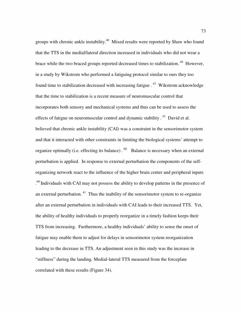
73

groups with chronic ankle instability.40

Mixed results were reported by Shaw who found

that the TTS in the medial/lateral direction increased in individuals who did not wear a

brace while the two braced groups reported decreased times to stabilization. 40

However,

in a study by Wikstrom who performed a fatiguing protocol similar to ours they too

found time to stabilization decreased with increasing fatigue . 41

Wikstrom acknowledge

that the time to stabilization is a recent measure of neuromuscular control that

incorporates both sensory and mechanical systems and thus can be used to assess the

effects of fatigue on neuromuscular control and dynamic stability . 41

David et al.

believed that chronic ankle instability (CAI) was a constraint in the sensorimotor system

and that it interacted with other constraints in limiting the biological systems’ attempt to

organize optimally (i.e. effecting its balance) . 60

Balance is necessary when an external

perturbation is applied. In response to external perturbation the components of the self-

organizing network react to the influence of the higher brain center and peripheral inputs

.60

Individuals with CAI may not possess the ability to develop patterns in the presence of

an external perturbation. 41

Thus the inability of the sensorimotor system to re-organize

after an external perturbation in individuals with CAI leads to their increased TTS. Yet,

the ability of healthy individuals to properly reorganize in a timely fashion keeps their

TTS from increasing. Furthermore, a healthy individuals’ ability to sense the onset of

fatigue may enable them to adjust for delays in sensorimotor system reorganization

leading to the decrease in TTS. An adjustment seen in this study was the increase in

“stiffness” during the landing. Medial-lateral TTS measured from the forceplate

correlated with these results (Figure 34).

74

Accelerometer Methodology Validation

Accelerometer temporal and spatial characteristics of magnitude and angular

orientation were used to test the validity of the device as a dynamic measurement tool. As

mentioned before, the correlation between vGRF and accelerometer magnitude was high

(r2=0.90), but the inverse relationship makes the accelerometer data unusable as a metric

for monitoring fatigue (Figure 36).

The temporal relationship between medial-lateral acceleration and medial-lateral

forceplate data was also found to be high (r2=1.00). The medial-lateral TTS did not have

a significant change associated with fatigue (Figure 32), but the trend was consistent with

previous research. The accelerometer may be an effective tool for monitoring this

variable.

The orientation data had a poor correlation when comparing kinematic data from

the shoe with derived angular data from the medial-lateral channel of the accelerometer

(Figure 39) (r2=0.37). This was probably due to the impact of linear (translational)

movement on the accelerometer aligned in the medial-lateral direction. It was hoped that

this movement would be minimal since the measurement was taken after the foot made

contact with the floor. The poor correlation suggests that this was not the case and that

the angular orientation data was contaminated by linear translation data.

The temporal relationship of angular movement would not be as sensitive to this

linear movement. The correlation of TTP angular accelerometer orientation with

kinematic frontal plane foot position (inversion/eversion) is good (Figure 40) (r2=0.85).

This is another variable that may be easily monitored via a shoe mounted accelerometer.

75

Accelerometer angular orientation and foot inversion were chosen because they

represent the rotation occurring at the ankle/foot joint. Increased rotation about this joint

puts strain on the lateral ankle ligaments (i.e. the anterior talofibular and calcaneofibular

ligaments). This can increase the potential for injury. The time to which the maximum

rotations occurred were analyzed and once again a strong correlation was established

between the two sets of temporal data.

The fact that there was such a strong correlation between the forceplate, kinematic

sensors, and accelerometer, justifies a need for further exploration of this device and

perhaps the inclusion of angular rate sensors that are insensitive to linear translations.

Due to the strong correlation between the temporal data between the devices and the fact

that the changes in time were associated with fatigue it implies that these changes can be

used to indicate ankle fatigue in individuals.

Hypotheses

H1: The hypothesis that medial-lateral time-to-stabilization (TTS) during the impact

phase of landing (0 to 200ms) will increase with lower extremity fatigue was found to be

false. It was postulated that the decrease in TTS associated with fatigue was a result of a

change in landing strategy, a shift toward the use of more proximal muscles (a hip

strategy).

H2: The hypothesis that ankle and hip joint torque during the impact phase of landing

(0 to 200ms) will increase with quadriceps muscle (knee joint) fatigue was found to be

false. Hip torque increased and ankle torque decreased. The ankle torque may have

76

decreased because the fatigue protocol did not isolate the quadriceps muscles. The use of

both proximal and distal joints is required when performing a squat. Anecdotally, some

subjects did describe a burning sensation in their plantar flexors as the protocol

progressed.

H3a: The hypothesis that accelerometer magnitude will be correlated with translational

kinetic data during landing was found to be true. However, it was inversely correlated

and may not be an appropriate indicator for monitoring fatigue.

H3b: The hypothesis that accelerometer rotational derivatives along an anterior-

posterior foot axis will be correlated with rotational kinetic data during landing was

found to be true. The temporal relationships may be the most sensitive to changes in

fatigue.

Conclusion

The jump landing protocol was successful in inducing quadriceps muscle fatigue.

This was confirmed by patterns in the vGRF and the sagittal/ frontal plane kinetics and

kinematics data. Additionally, the use of the accelerometer for measuring time to

stabilization was also found to be useful since the overall decrease in TTS was consistent

with an overall decrease in COP path length, area, and velocity. All of these

measurements characterize the dynamic stability at the foot and the ability of the

77

accelerometer to capture this measurement highlights its roles as a dynamic measurement

device.

This research demonstrates that a tri-axial accelerometer mounted in the heel of a

shoe can monitor some of the parameters known to change with lower extremity fatigue.

Although spatial correlations are not high, the temporal correlations may be sufficient to

warrant further exploration of the device. The addition of angular rate sensors may be the

next logical step in the development of the device.

78

References

1. Mohammadi F. Comparison of 3 preventive methods to reduce the recurrence of

ankle inversion sprains in male soccer players. Am J Sports Med. 2007;35(6):922-

926.

2. Konradsen L, Bech L, Ehrenbjerg M, Nickelsen T. Seven years follow-up after

ankle inversion trauma. Scan J Med Sci Sports. 2002;12(3):129-135.

3. Evans G, Hardcastle P, Frenyo A. Acute rupture of the lateral ligament of the

ankle: to suture or not to suture? J Bone Joint Surg Br. 1984;66:209-212.

4. Anandacoomarasamy A, Barnsley L. Long term outcomes of inversion ankle

injuries. Br J Sports Med. 2005;39(3).

5. Torg J. Athletic footwear and orthotic appliances. Clin Sports Med. 1982;1:157-

175.

6. Smith R, Reischl S. Treatment of ankle sprains in young athletes. Am J Sports

Med. 1986;14:465-471.

7. Freeman MAR, Dean MRE, Hanham IMF. The etiology and prevention of

functional instability of the foot. J Bone Joint Surg. 1965;47B:678-685.

8. Harrington KD. Degenerative arthritis of the ankle secondary to longstanding

lateral ligament instability. J Bone Joint Surg Am. 1979;61:354-361.

9. Gross P, Marti B. Risk of degenerative ankle joint disease in volleyball players:

study of former elite athletes. Int J Sports Med. 1999;20:58-63.

10. Verhagen RAW, de Keizer G, van Dijk CN. Long-term follow-up of inversion

trauma of the ankle. Arch Orthop Trauma Surg. 1995;114:92-96.

11. Schaap GR, de Keizer G, Marti K. Inversion trauma of the ankle. Arch Orthop

Trauma Surg. 1989;108:272-275.

12. Injury Surveillance System. Sport specific injury data. Available at:

<http://www1.ncaa.org/membership/ed_outreach/health-safety/iss/Reports2003-

04>.Accessed April 3, 2004.

79

13. Shaw MY, Gribble PA, Frye JL. Ankle Bracing, Fatigue, and Time to

Stabilization

in Collegiate Volleyball Athletes. J. of Athletic Training, 2008; 43(2): 164-71.

14. Salavanti M, Moghadam M, Ebrahimi, Arab AM. Changes in Postural Stability

with Fatigue of Lower Extremity Frontal and Sagittal Plane Movers. Gait &

Posture. 2007; 26: 214-218.

15. Madigan ML., Pidcoe P. Changes in Landing Biomechanics during a Fatiguing

Landing Activity. Journal of Electromyography and Kinesiology 2003; 13:491-

498.

16. DiStefano LJ, Padua DA, Brown CN, Guskiewicz KM. Lower Extremity

Kinematics and Ground Reaction Forces after Prophylactic Lace-Up Ankle

Bracing. J. Athletic Training. 2008; 43(3): 234-241.

17. Salci Y, Kentel BB, Heycan C, Akin S, Korkusuz F. Comparison of Landing

Maneuvers between Male and Female College Volleyball Players. Clin. Biomech.

2004; 19 (6): 622-628.

18. Myers JB, Riemann BL, Hwang J, Fu FU, and Lephart SM. Effect of Peripheral

Afferent Alteration of the Lateral Ankle Ligaments on Dynamic Stability. Am. J.

Sports Med. 2003; 31(4): 498-506.

19. Dubin J. Ankle Sprain/Twisted Ankle. Dubin Chiropractic 2003; 1(14).

20. Emedicine Cite: Craig C Young: Foot and Ankle.Emedicine.medscape.com

21. Alderton AK., Mortiz U. and R. Moe-Nilssen. Forceplate and Accelerometer

Measures for Evaluating the Effect of Muscle Fatigue on Postural Control During

One-Legged Stance. Physiotherapy Research International 2003; 8(4): 187-199.

22. Winter DA. Human Balance and Posture Control during Standing and Walking.

Gait

& Posture 1995; 3: 193-214.

23. Onell A. Quantifying Human Balance. Analysis of Forceplate Data. Uppsala:

Uppsala University, dissertation, 1999.

24. Weinhandl, J.T., Smith, J.D., Finch, W.H., & Dugan, E.L. Effects of repetitive

drop jumps on lower extremity landing mechanics. American Society of

Biomechanics Annual Meeting, Palo Alto, CA, August, 2007.

25. Benjamise, A. et.al. Fatigue Alters Lower Extremity Kinematics during a Single-

80

Leg Stop-Jump Task. Knee Surg Sports Traumatol. Arthrosc. 2008; 16:400-407.

26. Christina KA., White SC., and L. Gilchrist. Effect of Localized Muscle Fatique on

Vertical Ground Reaction Forces and Ankle Joint Motion during Running.

Human Movement Science 2001; 20: 257-276.

27. Nigg BM, Cole GK & Bruggemann GP. Impact forces during heel-toe running.

Journal of Applied Biomechanics, 1995; 11: 407-432.

28. Nyland JA, Shapiro R, Carbon DN, Nitz AJ, Malone TR. The Effect of

Quadriceps Femoris, Hamstring, and Placebo Eccentric Fatigue on Knee and

Ankle Dynamics during Crossover Cutting. Knee Surgery, Sports Traumatology,

Arthroscopy, 1997; 25: 171-184.

29. Gage H. Accelerographic analysis of Human Gait. Washington DC: American

Society for Mechanical Engineers, 1964.

30. Saunders J, Inman, V, Eberhart H. The Major Determinants in Normal and

Pathological Gait. J Bone Jnt Surg., 1953; 35A: 543-58.

31. Teramoto K, Dufek J, and John Mercer. The Effects of Local Muscle Fatigue on

Shock Attenuation for Female Runners. UNLV.

32. Voloshin A, Wosk J and Brull M. Force Wave Transmission through the Human

Locomotor System, Trans. Of the ASME. J of Biomechanical Eng., 1981; 100:

48-50.

33. Wosk J and Voloshin A. Wave Attenuation in Skeletons of Young Healthy

Persons. J Biomech.,1981; 14: 261-267.

34. Henriksen M., et.al. Test-Retest reliability of Trunk Accelerometric Gait

Analysis. Gait and Posture, 2004; 19: 288-297.

35. Culhane KM, O’Connor M, Lyons D, and G.M. Lyons. Age and Ageing:

Accelerometers in Rehabilitation Medicine for Older Adults. Age and Ageing,

2005; 34(6): 556-560.

36. Bouten CV, Westerterp KR, Verduin M, and J Janssen.Assessment of Energy

Expenditure for Physical Activity using a Triaxial Accelerometer.Med. Sci. in

Sports Exerc., 1994; 26 (12): 1516-1523.

37. Bates, Ostering & Sawhill, 1983 (In-shoe measurements article)

81

38. Oatis, Carol. Kinesiology: The Mechanics and Pathomechanics of Human

Movement. Philadelphia: Lippincott Williams & Wilkins, 2009.

39. Billing D. In-shoe Measurement for Biomechanical Monitoring.

40. Brown CA and Mynark R. Balance Deficits in Recreational Athletes with Chronic

Ankle Instability. J. of Athletic Training, 2007; 42(3):367-73.

41. Wikstrom EA, Powers ME, Tillman MD. Dynamic Stabilization Time After

Isokinetic and Functional Fatigue. J. of Athletic Training, 2004; 39(3): 247-53.

42. Forestier N, Teasdale N, Nougier V. Alteration of the Position Sense at the Ankle

Induced by Muscular Fatigue in Humans. Med. Sci. Sports Exercise, 2002;

34(1):117-22.

43. Johnston RB 3rd

, Howard ME, Cawley PW, Losse GM. Effect of Lower

Extremity Muscular Fatigue on Motor Control Performance. Med. Sci. Sports

Exercise, 1998; 30(12): 1703-7.

44. Ross SE and KM Guskiewicz. Examination of Static and Dynamic Postural

Stability in Individuals with Functionally Stable and Unstable Ankles. Clin. J.

Sports Med., 2004; 14(6): 332-338.

45. Freeman M, Dean M, Hanham I. The Etiology and Prevention of Functional

Stability of the Foot. J. Bone Joint Surg. Br., 1965; 47: 678-684.

46. Cordova ML, Ingersoll CD. Peroneus Longus Stretch Reflex Amplitude

Increases after Ankle Brace Application. Br. J. Sports Med., 2003; 37(3): 258-

262.

47. Cavanagh, PR. A Technique for Averaging Center of Pressure Paths from a Force

Platform. J Biomech., 1978; 11: 487-491.

48. Cho WH, Choi H. Center of Pressure (COP) during the Postural Balance Control

of High-Heeled Woman. Proceedings of 2005 IEEE. Sept. 2004: 2761-2764.

49. Winter D. A. B. C. (Anatomy, Biomechanics, Control) of Balance during

Standing

and Walking. Waterloo, Ontario: Waterloo Biomechanics Publisher; 1995.

50. Opila, KA, Wagner SS, Schiowitz S et. Al. Postural Alignment in Barefoot and

High-Heeled Stance. Spine, 1988; 13:542-7.

82

51. Harringe ML, Halvorsen K, Renstrom P,Werner S. Postural Control Measured as

the Center of Pressure Excursion in Young Female Gymnasts with Low

Back Pain or Lower Extremity Injury. Gait & Posture, 2008; 28: 38-45.

52. Robinovitch SN, Heller B, Lui A, and J Cortez. Effect of Strength and Speed on

Torque Development on Balance Recovery with the Ankle Strategy. J.

Neurophysiol. 2002; 88(2): 613-620.

53. Lees A. Methods of Impact Absorption when Landing from a Jump. Eng. Med.,

1981; 10(4): 207-211.

54. Devita P, Skelly WA. Effect of Landing Stiffness on Joint Kinetics and Energetics

in the Lower Extremity. Med. Sci. Sports Exerc., 1992; 24: 108-115.

55. Zhang SN, Bates BT, Dufek JS. Contributions of Lower Extremity joints to

Energy Dissipation during Landing. Med. Sci. Sports Exerc., 2000; 32: 812-819.

56. Coventry, E et. al. The Effect of Lower Extremity Fatigue on Shock Attenuation

during Single-Leg Landing. Clinical Biomechanics, 2006; 21: 1090-1097.

57. Wheeless, CR. “Stance Phase of Gait.” Wheeless Textbook of Orthopaedics.

2009. Data Trace Internet.12 Jul. 2009.

<http://www.wheelessonline.com/ortho/stance_phase_of_gait>.

58. LeVeau, BR. Biomechanics of Human Motion.Philadelphia:W.B. Saunders

Company, 1992.

59. Mclean et. al. Impact of Fatigue on Gender-Based High-Risk Landing Strategies.

Medicine & Science in Sports & Exercise, 2007; 39 (3):502-514.

60. David K, Glazier P, Araujo D, Bartlett R. Movement Systems as Dynamical

Systems: the Functional Role of Variability and its Implications for Sports

Medicine. Sports Med., 2003; 33:245-260.

83

APPENDIX A

Statistical Analyses

Analysis of Variance was used to compare the means of the response variable

(vGRF, hip joint flexion, knee joint flexion, etc.) at the eleven different levels of the

normalized time (0, 0.1, 0.2, 0.3, etc.) Hence, the analysis of variance (ANOVA) was

used to extend the two-sample t-test for testing the equality of the means of two

populations or factor levels to a more general null hypothesis of comparing the equality

of more than two means versus the alternative hypothesis of them not all being equal.

First, boxplots of the data were generated to explore the mean level of the

response variable at each normalized time level as well as the distributional

characteristics of the data at each normalized time level. As part of the ANOVA

investigation, the boxplots, also called the box-and-whisker plots, of the response

variable were generated at each normalized time interval level. In the plot, a line is

drawn across the box at the median. The bottom of the box is at Q1, the first quantile

(25th

percentile) and the top of the box is at Q3, the third quantile (75th

percentile). The

whiskers are the lines that extend from the top and bottom of the box to the adjacent

values. The adjacent values are the lowest and highest observations that are inside the

regions defined with the lower limit at Q1- 1.5 *(Q3-Q1) and the upper limit at Q3 +

1.5*(Q3-Q1). Outliers are points outside of the lower and upper limits and are plotted

with an asterick. If the data is normally distributed, the median line is in the middle of

84

the box and and the whiskers extend approximately the same distance from the top and

bottom of the box.

For the ANOVA test, the general assumption is that the data at each of the

normalized time interval levels are from a normal distribution with equal variances.

Hence, the boxplots of the data at each level should be similar in shape. Furthermore, if

the means of the data at the different levels are the same, then the median lines of the

boxplots should be about the same. Figure A.1 is a boxplot of the peak vGRF 200ms

after impact data values at the normalized time levels. The assumption of normality at

each of the normalized levels appears to be valid although there are outliers for the

normalized levels less than 0.7.

Normalized Time

Tim

es Body W

eight

10.90.80.70.60.50.40.30.20.10

4.5

4.0

3.5

3.0

2.5

Boxplot of Average Peak vGRF 200ms after Impact

Figure A.1: Boxplot of Maximum vGRF

Interval plots of the data provided a plot of the group means at the normalized

time levels with one standard error bar above and below the mean. These plots illustrate

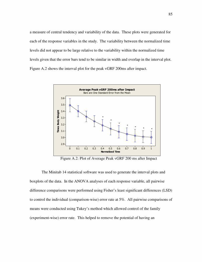
85

a measure of central tendency and variability of the data. These plots were generated for

each of the response variables in the study. The variability between the normalized time

levels did not appear to be large relative to the variability within the normalized time

levels given that the error bars tend to be similar in width and overlap in the interval plot.

Figure A.2 shows the interval plot for the peak vGRF 200ms after impact.

Normalized Time

Tim

es Body W

eight

10.90.80.70.60.50.40.30.20.10

3.6

3.5

3.4

3.3

3.2

3.1

3.0

2.9


Average Peak vGRF 200ms after Impact

*

*

**

** *

Figure A.2: Plot of Average Peak vGRF 200 ms after Impact

The Minitab 14 statistical software was used to generate the interval plots and

boxplots of the data. In the ANOVA analyses of each response variable, all pairwise

difference comparisons were performed using Fisher’s least significant differences (LSD)

to control the individual (comparison-wise) error rate at 5%. All pairwise comparisons of

means were conducted using Tukey’s method which allowed control of the family

(experiment-wise) error rate. This helped to remove the potential of having an

86

unexpectedly high probability of making at least one Type I error (declaring a difference

when there is none) among all the comparisons.

The One-Way ANOVA output consisted of an analysis of variance table, a table

of level means, individual 95% confidence intervals, the individual standard deviations

and the pooled standard deviation. The null hypothesis of no difference between means

is rejected if and only if zero is not contained in the confidence interval. The F-test p-

value is provided. Given that the alpha or significance level of the test is 0 .05, a p-value

less that 0.05 is an indication that the null hypothesis should be rejected and there is

evidence of differences among the means at the different normalized time interval levels.

The “HSU’s MCB” output compares each mean with the best of the other means.

For this study, the “best” level is the first or “un-fatigued” level. In some instances, the

un-fatigued level is the “smallest” mean level and all other levels will be compared with

the smallest mean. For others it is the “largest” mean level and all other mean levels with

be compared with the largest mean. All of these analyses were conducted for the

response variables in the study. The asterisks on the interval plot indicate that the

ANOVA results indicated that there was a significant difference in the mean level of the

peak vGRF values 200ms after impact at the “un-fatigued” normalized time (0) and the

normalized time levels of 0.4 and higher.

87

TABLE A.1

MINITAB ANOVA OUTPUT FOR PEAK VGRF 200ms AFTER IMPACT

One-way ANOVA: 0, 0.1, 0.2, 0.3, 0.4, 0.5, 0.6, 0.7, 0.8, 0.9, 1

Source DF SS MS F P

Factor 10 3.354 0.335 3.34 0.001

Error 121 12.159 0.100

Total 131 15.512

S = 0.3170 R-Sq = 21.62% R-Sq(adj) = 15.14%

Individual 95% CIs For Mean Based on

Pooled StDev

Level N Mean StDev -------+---------+---------+---------+--

0 12 3.4912 0.3451 (-------*------)

0.1 12 3.4011 0.2963 (------*------)

0.2 12 3.3202 0.2824 (------*------)

0.3 12 3.2485 0.2914 (------*------)

0.4 12 3.1860 0.3087 (------*-------)

0.5 12 3.1327 0.3243 (------*-------)

0.6 12 3.0885 0.3332 (-------*------)

0.7 12 3.0535 0.3339 (------*------)

0.8 12 3.0277 0.3279 (------*------)

0.9 12 3.0111 0.3198 (------*-------)

1 12 3.0037 0.3179 (------*------)

-------+---------+---------+---------+--

3.00 3.25 3.50 3.75

Pooled StDev = 0.3170

Hsu's MCB (Multiple Comparisons with the Best)

Family error rate = 0.05

Critical value = 2.48

Intervals for level mean minus largest of other level means

Level Lower Center Upper ---+---------+---------+---------+------

0 -0.2306 0.0901 0.4108 (---------*--------)

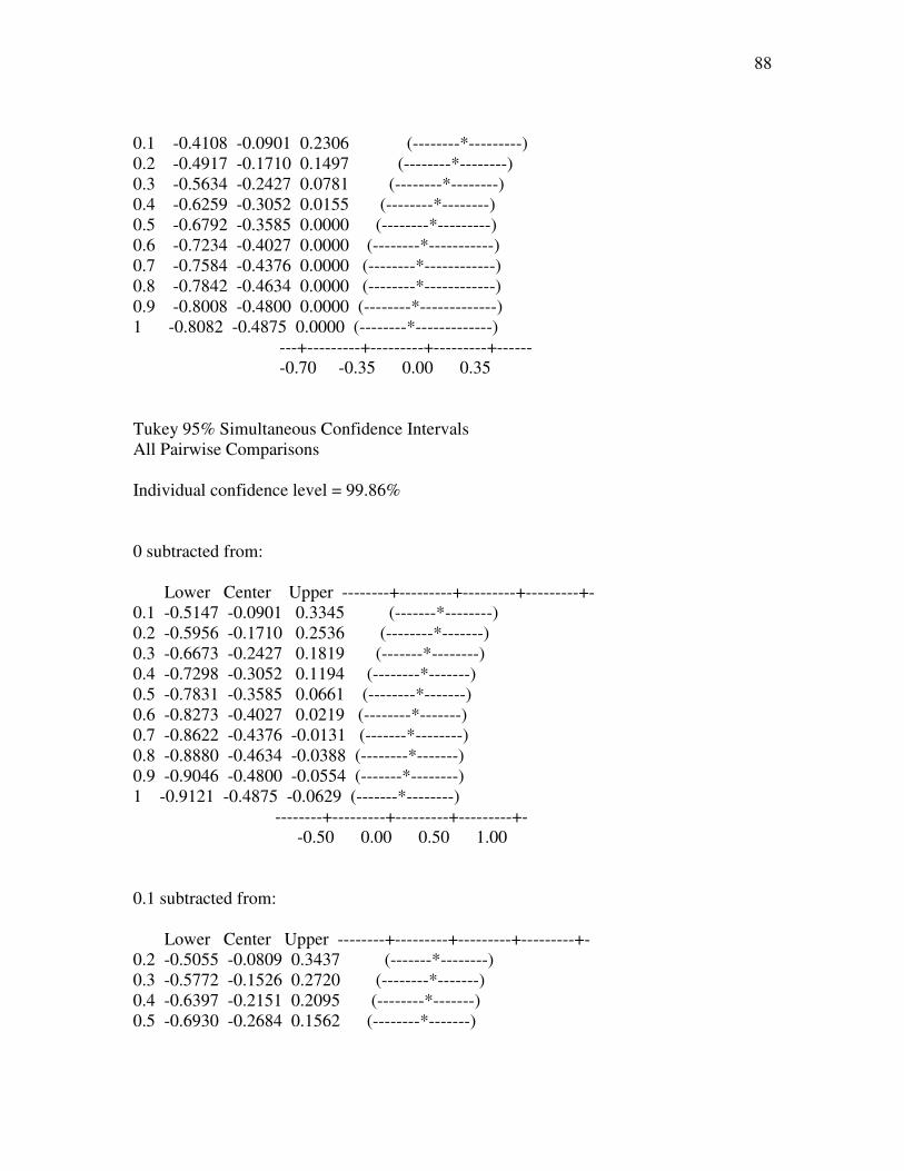
88

0.1 -0.4108 -0.0901 0.2306 (--------*---------)

0.2 -0.4917 -0.1710 0.1497 (--------*--------)

0.3 -0.5634 -0.2427 0.0781 (--------*--------)

0.4 -0.6259 -0.3052 0.0155 (--------*--------)

0.5 -0.6792 -0.3585 0.0000 (--------*---------)

0.6 -0.7234 -0.4027 0.0000 (--------*-----------)

0.7 -0.7584 -0.4376 0.0000 (--------*------------)

0.8 -0.7842 -0.4634 0.0000 (--------*------------)

0.9 -0.8008 -0.4800 0.0000 (--------*-------------)

1 -0.8082 -0.4875 0.0000 (--------*-------------)

---+---------+---------+---------+------

-0.70 -0.35 0.00 0.35

Tukey 95% Simultaneous Confidence Intervals

All Pairwise Comparisons

Individual confidence level = 99.86%

0 subtracted from:

Lower Center Upper --------+---------+---------+---------+-

0.1 -0.5147 -0.0901 0.3345 (-------*--------)

0.2 -0.5956 -0.1710 0.2536 (--------*-------)

0.3 -0.6673 -0.2427 0.1819 (-------*--------)

0.4 -0.7298 -0.3052 0.1194 (--------*-------)

0.5 -0.7831 -0.3585 0.0661 (--------*-------)

0.6 -0.8273 -0.4027 0.0219 (--------*-------)

0.7 -0.8622 -0.4376 -0.0131 (-------*--------)

0.8 -0.8880 -0.4634 -0.0388 (--------*-------)

0.9 -0.9046 -0.4800 -0.0554 (-------*--------)

1 -0.9121 -0.4875 -0.0629 (-------*--------)

--------+---------+---------+---------+-

-0.50 0.00 0.50 1.00

0.1 subtracted from:


0.2 -0.5055 -0.0809 0.3437 (-------*--------)

0.3 -0.5772 -0.1526 0.2720 (--------*-------)

0.4 -0.6397 -0.2151 0.2095 (--------*-------)

0.5 -0.6930 -0.2684 0.1562 (--------*-------)

89

0.6 -0.7372 -0.3126 0.1120 (--------*-------)

0.7 -0.7722 -0.3476 0.0770 (-------*--------)

0.8 -0.7980 -0.3734 0.0512 (--------*-------)

0.9 -0.8146 -0.3900 0.0346 (-------*--------)

1 -0.8220 -0.3974 0.0272 (-------*--------)

--------+---------+---------+---------+-

-0.50 0.00 0.50 1.00



0.3 -0.4963 -0.0717 0.3529 (--------*-------)

0.4 -0.5588 -0.1342 0.2904 (-------*--------)

0.5 -0.6121 -0.1875 0.2371 (-------*--------)

0.6 -0.6563 -0.2317 0.1929 (-------*--------)

0.7 -0.6913 -0.2667 0.1579 (--------*-------)

0.8 -0.7171 -0.2925 0.1321 (-------*--------)

0.9 -0.7337 -0.3091 0.1155 (--------*-------)

1 -0.7411 -0.3165 0.1081 (--------*-------)

--------+---------+---------+---------+-

-0.50 0.00 0.50 1.00



0.4 -0.4871 -0.0625 0.3621 (--------*-------)

0.5 -0.5404 -0.1158 0.3088 (--------*-------)

0.6 -0.5846 -0.1600 0.2646 (--------*-------)

0.7 -0.6196 -0.1950 0.2296 (-------*--------)

0.8 -0.6454 -0.2208 0.2038 (--------*-------)

0.9 -0.6620 -0.2374 0.1872 (-------*--------)

1 -0.6694 -0.2448 0.1798 (-------*--------)

--------+---------+---------+---------+-

-0.50 0.00 0.50 1.00



0.5 -0.4779 -0.0533 0.3713 (--------*-------)

0.6 -0.5221 -0.0975 0.3271 (-------*--------)

0.7 -0.5571 -0.1325 0.2921 (-------*--------)

90

0.8 -0.5828 -0.1582 0.2663 (--------*-------)

0.9 -0.5995 -0.1749 0.2497 (--------*-------)

1 -0.6069 -0.1823 0.2423 (-------*--------)

--------+---------+---------+---------+-

-0.50 0.00 0.50 1.00



0.6 -0.4688 -0.0442 0.3804 (-------*--------)

0.7 -0.5037 -0.0791 0.3454 (-------*--------)

0.8 -0.5295 -0.1049 0.3197 (--------*-------)

0.9 -0.5461 -0.1215 0.3031 (--------*-------)

1 -0.5536 -0.1290 0.2956 (-------*--------)

--------+---------+---------+---------+-

-0.50 0.00 0.50 1.00



0.7 -0.4596 -0.0350 0.3896 (-------*--------)

0.8 -0.4853 -0.0608 0.3638 (--------*-------)

0.9 -0.5020 -0.0774 0.3472 (-------*--------)

1 -0.5094 -0.0848 0.3398 (-------*--------)

--------+---------+---------+---------+-

-0.50 0.00 0.50 1.00



0.8 -0.4504 -0.0258 0.3988 (-------*--------)

0.9 -0.4670 -0.0424 0.3822 (-------*--------)

1 -0.4744 -0.0498 0.3748 (-------*-------)

--------+---------+---------+---------+-

-0.50 0.00 0.50 1.00



0.9 -0.4412 -0.0166 0.4080 (--------*-------)

91

1 -0.4486 -0.0240 0.4006 (--------*-------)

--------+---------+---------+---------+-

-0.50 0.00 0.50 1.00



1 -0.4320 -0.0074 0.4172 (--------*-------)

--------+---------+---------+---------+-

-0.50 0.00 0.50 1.00

Fisher 95% Individual Confidence Intervals

All Pairwise Comparisons

Simultaneous confidence level = 33.69%

0 subtracted from:

Lower Center Upper -+---------+---------+---------+--------

0.1 -0.3463 -0.0901 0.1661 (------*-------)

0.2 -0.4272 -0.1710 0.0852 (------*------)

0.3 -0.4989 -0.2427 0.0135 (------*------)

0.4 -0.5614 -0.3052 -0.0490 (------*-------)

0.5 -0.6147 -0.3585 -0.1023 (-------*------)

0.6 -0.6589 -0.4027 -0.1465 (------*-------)

0.7 -0.6939 -0.4376 -0.1814 (------*-------)

0.8 -0.7196 -0.4634 -0.2072 (-------*------)

0.9 -0.7362 -0.4800 -0.2238 (------*-------)

1 -0.7437 -0.4875 -0.2313 (------*------)

-+---------+---------+---------+--------

-0.70 -0.35 0.00 0.35



0.2 -0.3371 -0.0809 0.1753 (-------*------)

0.3 -0.4088 -0.1526 0.1036 (-------*------)

0.4 -0.4713 -0.2151 0.0411 (------*------)

0.5 -0.5246 -0.2684 -0.0122 (------*-------)

0.6 -0.5688 -0.3126 -0.0564 (------*------)

92

0.7 -0.6038 -0.3476 -0.0914 (------*------)

0.8 -0.6296 -0.3734 -0.1172 (------*-------)

0.9 -0.6462 -0.3900 -0.1338 (------*------)

1 -0.6536 -0.3974 -0.1412 (-------*------)

-+---------+---------+---------+--------

-0.70 -0.35 0.00 0.35



0.3 -0.3279 -0.0717 0.1845 (------*------)

0.4 -0.3904 -0.1342 0.1220 (------*------)

0.5 -0.4437 -0.1875 0.0687 (-------*------)

0.6 -0.4879 -0.2317 0.0245 (------*-------)

0.7 -0.5229 -0.2667 -0.0105 (------*-------)

0.8 -0.5487 -0.2925 -0.0363 (-------*------)

0.9 -0.5653 -0.3091 -0.0529 (------*------)

1 -0.5727 -0.3165 -0.0603 (------*------)

-+---------+---------+---------+--------

-0.70 -0.35 0.00 0.35



0.4 -0.3187 -0.0625 0.1937 (------*-------)

0.5 -0.3720 -0.1158 0.1404 (-------*------)

0.6 -0.4162 -0.1600 0.0962 (------*-------)

0.7 -0.4512 -0.1950 0.0612 (------*-------)

0.8 -0.4770 -0.2208 0.0354 (-------*------)

0.9 -0.4936 -0.2374 0.0188 (------*-------)

1 -0.5010 -0.2448 0.0114 (------*------)

-+---------+---------+---------+--------

-0.70 -0.35 0.00 0.35



0.5 -0.3095 -0.0533 0.2029 (------*-------)

0.6 -0.3537 -0.0975 0.1587 (------*-------)

0.7 -0.3887 -0.1325 0.1237 (------*-------)

0.8 -0.4145 -0.1582 0.0980 (------*-------)

93

0.9 -0.4311 -0.1749 0.0813 (------*------)

1 -0.4385 -0.1823 0.0739 (-------*------)

-+---------+---------+---------+--------

-0.70 -0.35 0.00 0.35



0.6 -0.3004 -0.0442 0.2120 (-------*------)

0.7 -0.3354 -0.0791 0.1771 (-------*------)

0.8 -0.3611 -0.1049 0.1513 (------*------)

0.9 -0.3777 -0.1215 0.1347 (-------*------)

1 -0.3852 -0.1290 0.1272 (------*-------)

-+---------+---------+---------+--------

-0.70 -0.35 0.00 0.35



0.7 -0.2912 -0.0350 0.2212 (------*------)

0.8 -0.3170 -0.0608 0.1955 (------*-------)

0.9 -0.3336 -0.0774 0.1788 (-------*------)

1 -0.3410 -0.0848 0.1714 (-------*------)

-+---------+---------+---------+--------

-0.70 -0.35 0.00 0.35



0.8 -0.2820 -0.0258 0.2304 (------*-------)

0.9 -0.2986 -0.0424 0.2138 (-------*------)

1 -0.3060 -0.0498 0.2064 (-------*------)

-+---------+---------+---------+--------

-0.70 -0.35 0.00 0.35



0.9 -0.2728 -0.0166 0.2396 (-------*------)

1 -0.2802 -0.0240 0.2322 (------*-------)

94

-+---------+---------+---------+--------

-0.70 -0.35 0.00 0.35



1 -0.2636 -0.0074 0.2488 (-------*------)

-+---------+---------+---------+--------

-0.70 -0.35 0.00 0.35

Reference

MINITAB Reference Manual, Release 14, MINITAB Inc., July 2004.

95

APPENDIX B

The following pages contain a printout of the customized MATLABTM

software

used to perform the analysis in this study.

Matlab Code

clear

close all

%Baseline Data %%%%%%%%%%%%%%%%%%%%%%%%%%%%%%%%%%%

Wt=86.20; %kg

Ht=1.71; %meters

tbw=Wt*9.81; %Newtons

WtHt=Wt*Ht;

%%%%%%%%%%%%%%%%%%%%%%%%%%%%%%%%%%%%%%%%%%%

data0=xlsread('ts050109a_0');

Frame0=data0(:,1); Hip0=data0(:,2); Knee0=data0(:,3); Ankle0=data0(:,4);

Foot0=data0(:,5); SacHt0=data0(:,6); ThighSM0=data0(:,7); ShankSM0=data0(:,8);

FootSM0=data0(:,9);

ThighFP0=data0(:,10); ShankFP0=data0(:,11); FootFP0=data0(:,12);

ThighFM0=data0(:,13); ShankFM0=data0(:,14); FootFM0=data0(:,15);

Accx0=data0(:,16);Accy0=data0(:,17);Accz0=data0(:,18);

fpm0=data0(:,19);fpx0=data0(:,20); fpy0=data0(:,21); fpAPM0=data0(:,22);

fpz0=data0(:,23);

%Orientation

%%%%%%%%%%%%%%%%%%%%%%%%%%%%%%%%%%%%%%%%%%%

OrientMatrix=[0.865, 0.211,0.453;0.011,0.948,0.317;-0.224,-0.052,0.974];

AccX0=((Accx0-1.5)./.3).*tbw;

AccY0=((Accy0-1.5)./.3).*tbw;

AccZ0=((Accz0-1.5)./.3).*tbw;

AccMag0=sqrt(((AccX0).^2)+((AccY0).^2)+((AccZ0).^2));

VectorMatrix0=[AccX0,AccY0,AccZ0];

AccXX0=AccX0./tbw;AccYY0=AccY0./tbw;AccZZ0=AccZ0./tbw;

Vector0=VectorMatrix0*OrientMatrix;

VectorX0=Vector0(:,1);VectorY0=Vector0(:,2);VectorZ0=Vector0(:,3);

VecSquared0=sqrt((VectorX0.^2)+(VectorY0.^2)+(VectorZ0.^2));

VecNormX0=VectorX0./VecSquared0;

VecNormY0=VectorY0./VecSquared0;

VecNormZ0=VectorZ0./VecSquared0;

96

AngleX0=asind(VecNormX0(1:500));

%Averages %%%%%%%%%%%%%%%%%%%%%%%%%%%%%%%%%%%

AvgHip0=mean(Hip0);

AvgKnee0=mean(Knee0);

97

AvgAnkle0=mean(Ankle0);

AvgFoot0=mean(Foot0);

AvgCorVecNormX=mean(VecNormX0);

AvgCorVecNormY=mean(VecNormY0);

AvgCorVecNormZ=mean(VecNormZ0);

%%%%%%%%%%%%%%%%%%%%%%%%%%%%%%%%%%%%%%%%%%%

jump=37;

for i=1:jump

filename=['ts050109a_',num2str(i)];

data=xlsread(filename);

Frame=data(:,1); Hip=data(:,2); Knee=data(:,3); Ankle=data(:,4);

Foot=data(:,5); SacHt=data(:,6); ThighSM=data(:,7); ShankSM=data(:,8);

FootSM=data(:,9);

ThighFP=data(:,10); ShankFP=data(:,11); FootFP=data(:,12);

ThighFM=data(:,13); ShankFM=data(:,14); FootFM=data(:,15);

Accx=data(:,16);Accy=data(:,17);Accz=data(:,18);

fpm=data(:,19);fpx=data(:,20); fpy=data(:,21); fpAPM=data(:,22);

fpz=data(:,23);

LF=length(Frame);

for j=1:LF

AccX(j)=((Accx(j)-1.5)./.3).*tbw;

AccY(j)=((Accy(j)-1.5)./.3).*tbw;

AccZ(j)=((Accz(j)-1.5)./.3).*tbw;

AccMag(j)=sqrt(((AccX(j)).^2)+((AccY(j)).^2)+((AccZ(j)).^2));

if j>2

if fpz(j-1)==0 && fpz(j)>1

contacttime(i)=j;

end

end

end

%%%%%%%%%%%%%%%%%%%%%%%%%%%%%%%%%%%%%%%%%%%

range200=contacttime(i):contacttime(i)+200;




range450=contacttime(i)+55:contacttime(i)+555;

range415=contacttime(i)+15:contacttime(i)+515;

98

lr=length(range500);

%%%Accelerometer%%%%%%%%%%%%%%%%%%%%%%%%%%%%%%%%%

AccelX(:,i)=((AccX)/tbw)';

AccelY(:,i)=((AccY)/tbw)';

AccelZ(:,i)=((AccZ)/tbw)';

AccelMag(:,i)=sqrt(((AccelX(range415,i)).^2)+((AccelY(range415,i)).^2)+((AccelZ(rang

e415,i)).^2));

[peakAccMag(i),peakAccMagtime(i)]=max(AccelMag(:,i));

%%%%%%%%%%%%%%%%%%%%%%%%%%%%%%%%%%%%%%%%%%%

VectorMatrix=[AccelX(range500,i),AccelY(range500,i),AccelZ(range500,i)];

AccelXvec(:,i)=AccelX(range500,i);

AccelYvec(:,i)=AccelY(range500,i);

AccelZvec(:,i)=AccelZ(range500,i);

AccelMagvec(:,i)=AccelMag(:,i);

%VectorMatrix=[Accx(range500),Accy(range500),Accz(range500)]; %original

Vector=VectorMatrix*OrientMatrix;

VectorX=Vector(:,1);

VectorY=Vector(:,2);

VectorZ=Vector(:,3);

VecSquared=sqrt((VectorX.^2)+(VectorY.^2)+(VectorZ.^2));

VecNormX(:,i)=VectorX./VecSquared;

VecNormY(:,i)=VectorY./VecSquared;

VecNormZ(:,i)=VectorZ./VecSquared;

%Vector=VectorMatrix*OrientMatrix;

[peakAccelX(i),timepeakAccelX(i)]=max(AccelX(range500,i)); %G's

[peakVecNormX(i),timepeakVecNormX(i)]=max(VecNormX(:,i)); %G's

NormXVecGs(:,i)=((VecNormX(:,i))-1.5/0.3); %G's

%%%%%%%%%%%%%%%%%%%%%%%%%%%%%%%%%%%%%%%%%%%

[MaxangleVecNormXs(i),TimeMaxangleVecNormXs(i)]=max(asind(VecNormX(1:200,i

)));

[MinangleVecNormXs(i),TimeMinangleVecNormXs(i)]=min(asind(VecNormX(1:200,i)

));

AngleX(:,i)=(asind(VecNormX(1:500,i)));

%Accelerometer Derivative/Jerk Calculation%%%%%%%%%%%%%%%%%%%%%

DiffAccX(:,i)=diff(AccelXvec(:,i));

DiffAccY(:,i)=diff(AccelYvec(:,i));

DiffAccZ(:,i)=diff(AccelZvec(:,i));

DiffAccelX(:,i)=diff(VecNormX(:,i));

DiffAccelY(:,i)=diff(VecNormY(:,i));

DiffAccelZ(:,i)=diff(VecNormZ(:,i));

99

ContactTime(i)=contacttime(i);

%Ground Force Reaction(vGRF)Ranges

%%%%%%%%%%%%%%%%%%%%%%%%%%%%%%%%%%%%%%%%%%%

fpmag(:,i)=fpm(range500)/tbw;

[maxfpmag(i),maxtimefpmag(i)]=max(fpm(range500)/tbw);

[minfpmag(i),mintimefpmag(i)]=min(fpm(range500)/tbw);

fpZ(:,i)=fpz;

fpZ200(:,i)=fpZ(range200);

fpZ500(:,i)=fpZ(range500);

FPZ(:,i)=fpz/tbw;

FPZ200(:,i)=FPZ(range200);

FPZ500(:,i)=FPZ(range500);

%Peak

vGRF%%%%%%%%%%%%%%%%%%%%%%%%%%%%%%%%%%%%%%%%

[vGRFpeak(i),vGRFpeaktime(i)]=max(FPZ(range200,i));

%Max Loading Rate%%%%%%%%%%%%%%%%%%%%%%%%%%%%%%%%%

[Rise,Run]=max(fpZ(range200,i));

RiseKN=Rise/1000;

RunS=Run/1000;

maxloadrate(i)=(RiseKN/RunS);

%Impulse: vGRF %%%%%%%%%%%%%%%%%%%%%%%%%%%%%%%%%%

vGRFImp(i)=trapz((FPZ(range200,i))*0.001);

%Time to Stabilization%%%%%%%%%%%%%%%%%%%%%%%%%%%%%%%%

AvgCorVecX=mean(VecNormX0);

diffCorVecX(:,i)=(VecNormX(:,i))-AvgCorVecX;%

StdX(i)=std(diffCorVecX(:,i));

AvgCorVecY=mean(VecNormY0);

diffCorVecY(:,i)=(VecNormY(:,i))-AvgCorVecY;

StdY(i)=std(diffCorVecY(:,i));

AvgCorVecZ=mean(VecNormZ0);

diffCorVecZ(:,i)=(VecNormZ(:,i))-AvgCorVecZ;

StdZ(i)=std(diffCorVecZ(:,i));

for m=1:500

if abs(diffCorVecX(m,i))>=StdX(i)

ttsoutx(m,i)=1;

if ttsoutx(m,i)==1

100

ttscountx(i)=m;

end

else

ttsoutx(m,i)=0;

end

if abs(diffCorVecY(m,i))>=StdY(i)

ttsouty(m,i)=1;

if ttsouty(m,i)==1

ttscounty(i)=m;

end

else

ttsouty(m,i)=0;

end

if abs(diffCorVecZ(m,i))>=StdZ(i)

ttsoutz(m,i)=1;

if ttsoutz(m,i)==1

ttscountz(i)=m;

end

else

ttsoutz(m,i)=0;

end

end

%Flexion(degrees): Hip, Knee and Ankle%%%%%%%%%%%%%%%%%%%%%%%

HipZeroed(:,i)=Hip-AvgHip0;

KneeZeroed(:,i)=Knee-AvgKnee0;

AnkleZeroed(:,i)=Ankle-AvgAnkle0;

FootZeroed(:,i)=Foot-AvgFoot0;

[HipMaxFlex(i),HipMaxFlexTime(i)]=max(HipZeroed(range500,i));

[KneeMaxFlex(i),KneeMaxFlexTime(i)]=max(KneeZeroed(range500,i));

[AnkleMaxFlex(i),AnkleMaxFlexTime(i)]=max(AnkleZeroed(range500,i));

[footMaxInv(i),footMaxInvTime(i)]=max(FootZeroed(range200,i));

[footMinInv(i),footMinInvTime(i)]=min(FootZeroed(range200,i));

HipZ(:,i)=HipZeroed(range500,i);

KneeZ(:,i)=KneeZeroed(range500,i);

AnkleZ(:,i)=AnkleZeroed(range500,i);

FootZ(:,i)=FootZeroed(range500,i);

%Saggital Plane Moments &

Impulses%%%%%%%%%%%%%%%%%%%%%%%%%%%%%%%%%%%%%%

%%%

ThighSM(:,i)=ThighSM/WtHt;

101

ThighSM500(:,i)=ThighSM(range500,i);

[ThighSMPeak(i),ThighSMTime(i)]=max(ThighSM(range200,i));

ThighSMImp(i)=trapz(ThighSM(range200,i))*0.001;%*0.2;

ShankSM(:,i)=ShankSM/WtHt;

ShankSM500(:,i)=ShankSM(range500,i);

[ShankSMPeak(i),ShankSMTime(i)]=max(ShankSM(range200,i));

ShankSMImp(i)=trapz(ShankSM(range200,i))*0.001;

FootSM(:,i)=FootSM/WtHt;

FootSM500(:,i)=FootSM(range500,i);

[FootSMPeak(i),FootSMTime(i)]=max(FootSM(range200,i));

FootSMImp(i)=trapz(FootSM(range200,i))*0.001;

%Frontal Plane Moments &

Impulses%%%%%%%%%%%%%%%%%%%%%%%%%%%%%%%%%%%%%%

ThighFM(:,i)=ThighFM/WtHt;

ThighFM500(:,i)=ThighFM(range500,i);

[ThighFMPeak(i),ThighFMTime(i)]=max(ThighFM(range200,i));

ThighFMImp(i)=trapz(ThighFM(range200,i))*0.001;

ShankFM(:,i)=ShankFM/WtHt;

ShankFM500(:,i)=ShankFM(range500,i);

[ShankFMPeak(i),ShankFMTime(i)]=max(ShankFM(range200,i));

ShankFMImp(i)=trapz(ShankFM(range200,i))*0.001;

FootFM(:,i)=FootFM/WtHt;

FootFM500(:,i)=FootFM(range500,i);

[FootFMPeak(i),FootFMTime(i)]=max(FootFM(range200,i));

FootFMImp(i)=trapz(FootFM(range200,i))*0.001;

%Sacral Height%%%%%%%%%%%%%%%%%%%%%%%%%%%%%%%%%%%

aSacHt(:,i)=abs(SacHt);

[MaxSacHt(i),MaxSacHtTime(i)]=max(aSacHt(:,i));

%Center of Pressure%%%%%%%%%%%%%%%%%%%%%%%%%%%%%%%%%

copx(:,i)=fpx(range200);

diffx(:,i)=abs(diff(copx(:,i)));

pathlengthx(i)=sum(diffx(:,i));

[maxcopx(i)]=max(copx(:,i));

[mincopx(i)]=min(copx(:,i));

rangex(i)=maxcopx(i)-mincopx(i);

102

copy(:,i)=fpy(range200)';

diffy(:,i)=abs(diff(copy(:,i)));

pathlengthy(i)=sum(diffy(:,i));

[maxcopy(i)]=max(copy(:,i));

[mincopy(i)]=min(copy(:,i));

rangey(i)=maxcopy(i)-mincopy(i);

coparea(i)=rangex(i)*rangey(i);

coppathlength(i)=(sqrt(((pathlengthx(i)).^2)+((pathlengthy(i)).^2)));

copvelocity(i)=coppathlength(i)/0.2;

%%Moment

about%%Y%%%%%%%%%%%%%%%%%%%%%%%%%%%%%%%%%%%%%

%%%%%%%%%%%%%%%%%%%%%

fPAPM(:,i)=(fpAPM(range500))/tbw;

mm=1:500;

fPAPM500(:,i)=fPAPM(:,i);

StdFP(i)=std(fPAPM500(:,i));

for mm=1:500

if abs(fPAPM500(mm,i))>=StdFP(i)

fpapmout(mm,i)=1;

if fpapmout(mm,i)==1

fpapmnumber(i)=mm;

end

else

fpapmout(mm,i)=0;

end

end

%Data Derivatives%%%%%%%%%%%%%%%%%%%%%%%%%%%%%%%%%

diffFPX(:,i)=diff(FPZ500(:,i));

Difffpapm(:,i)=diff(fPAPM(:,i));

%%%%%%%%%%%%%%%%%%%%%%%%%%%%%%%%%%%%%%%%%%%

normtime(i)=((i-1)/(jump-1));

%%%%%%%%%%%%%%%%%%%%%%%%%%%%%%%%%%%%%%%%%%%

figure(1)

ylim=[0 70];

for a=i

x=[HipMaxFlexTime(a) HipMaxFlexTime(a)] ;

plot(x,ylim)

hold on

plot(HipZ(:,a))

103

title(['Hip FlexionTrial',num2str(a)])

drawnow;

trial(i)=a;

end

figure(2)

ylim=[0 70];

for a=i

x=[KneeMaxFlexTime(a) KneeMaxFlexTime(a)] ;

plot(x,ylim)

hold on

plot(KneeZ(:,a))

title(['Knee Flexion Trial',num2str(a)])

drawnow;

trial(i)=a;

end

figure(3)

ylim=[-50 40];

for a=i

x=[AnkleMaxFlexTime(a) AnkleMaxFlexTime(a)] ;

plot(x,ylim)

hold on

plot(AnkleZ(:,a))

title(['Ankle Flexion Trial',num2str(a)])

drawnow;

trial(i)=a;

end

figure(4)

ylim=[0 2];

for a=i

x=[MaxSacHtTime(a) MaxSacHtTime(a)] ;

plot(x,ylim)

hold on

plot(aSacHt(:,a))

title(['Sacral Height Trial',num2str(a)])

drawnow;

trial(i)=a;

end

104

figure(5)

ylim=[0 6];

for a=i

x=[peakAccMagtime(a) peakAccMagtime(a)];

plot(x,ylim)

hold on

plot(AccelMag(:,a))

title(['Peak Accel Mag',num2str(a)])

drawnow;

trial(i)=a;

end

figure(6)

PeakVGRF(:,i)=(FPZ(range200,i));

ylim=[0 4];

for a=i

x=[vGRFpeaktime(a) vGRFpeaktime(a)];

plot(x,ylim)

hold on

plot(PeakVGRF(:,a))

title(['vGRF Trial',num2str(a)])

drawnow;

trial(i)=a;

end

trial(i)=i;

end

vGRF Data%%%%%%%%%%%%%%%%%%%%%%%%%%%%%%%%%%%

Trial=trial';

PEAKvGRFtime=vGRFpeaktime';

PEAKvGRF=vGRFpeak';

vPeak=vGRFpeak';

vGRFStoreTrialTimePeak=[Trial,PEAKvGRFtime,PEAKvGRF]

%%%%%%%%%%%%%%%%%%%%%%%%%%%%%%%%%%%%%%%%%

Trial=trial';

peakAccMag=peakAccMag';

peakAccMagtime=peakAccMagtime';

PeakAccMagStoreTrialTimePeak=[Trial,peakAccMagtime,peakAccMag]

%Hip Flex Data%%%%%%%%%%%%%%%%%%%%%%%%%%%%%%%%%%%

Trial=trial';

HipMaxFlexTime=HipMaxFlexTime';

HipMaxFlex=HipMaxFlex';

105

HipFlexStoreTrialTimePeak=[Trial,HipMaxFlexTime,HipMaxFlex]

%Knee Flex Data%%%%%%%%%%%%%%%%%%%%%%%%%%%%%%%%%

KneeMaxFlexTime=KneeMaxFlexTime';

KneeMaxFlex=KneeMaxFlex';

KneeFlexStoreTrialTimePeak=[Trial,KneeMaxFlexTime,KneeMaxFlex]

%Ankle Flex Data%%%%%%%%%%%%%%%%%%%%%%%%%%%%%%%%%%

Trial=trial';

AnkleMaxFlexTime=AnkleMaxFlexTime';

AnkleMaxFlex=AnkleMaxFlex';

AnkleFlexStoreTrialTimePeak=[Trial,AnkleMaxFlexTime,AnkleMaxFlex]

%Sacral Height%%%%%%%%%%%%%%%%%%%%%%%%%%%%%%%%%

Trial=trial';

MaxSacHtTime=MaxSacHtTime';

MaxSacHt=MaxSacHt';

MaxSacHtStoreTrialTimePeak=[Trial,MaxSacHtTime,MaxSacHt]

%%%%%%%%%%%%%%%%%%%%%%%%%%%%%%%%%%%%%%%%%%

AvgHip0=mean(Hip0)

AvgKnee0=mean(Knee0)

AvgAnkle0=mean(Ankle0)

AvgFoot0=mean(Foot0)

%%%%%%%%%%%%%%%%%%%%%%%%%%%%%%%%%%%%%%%%%%%

initialvPeak=vPeak

figure(7)

NormTime=normtime';

pvPeak=polyfit(NormTime,vPeak,2);

pvalvPeak=polyval(pvPeak,NormTime);

plot(NormTime,vPeak,'g')

hold on

plot(NormTime,pvalvPeak,'k')

pvPeak1=pvPeak(1);

pvPeak2=pvPeak(2);

pvPeak3=pvPeak(3);

j=0;

for n=1:11

yvPeak(n)=(pvPeak1*((j)^2))+(pvPeak2*(j))+(pvPeak3);

xdata(n)=j;

j=j+0.1;

end

106

VPEAK=yvPeak'

xlabel('Normalized Time')

ylabel('Times BW')

title('vGRF Peak')

legend('Raw Data','2nd Order Polynomial Fit')

%%%%%%%%%%%%%%%%%%%%%%%%%%

for g=1:length(vPeak)

if vPeak(g)>=6

vPeak(g)=(vPeak(g-1)+vPeak(g+1))/2;

end

end

newvPeak=vPeak

figure(8)

NormTime=normtime';

pnewvPeak=polyfit(NormTime,newvPeak,2);

pvalnewvPeak=polyval(pnewvPeak,NormTime);

plot(NormTime,newvPeak,'g')

hold on

plot(NormTime,pvalnewvPeak,'k')

pnewvPeak1=pnewvPeak(1);



j=0;

for n=1:11

ynewvPeak(n)=(pnewvPeak1*((j)^2))+(pnewvPeak2*(j))+(pnewvPeak3);

xdata(n)=j;

j=j+0.1;

end

NEWVPEAK=ynewvPeak'


ylabel('Times BW')

title('NEW vGRF Peak')


%%%%%%%%%%%%%%%%%%%%%%%%%%%%%%%%%%%%%%%%%%%

figure(9)

vGRFImpAll=vGRFImp';

ImpG=vGRFImpAll;

107

OldImpG=ImpG

pImpG=polyfit(NormTime,ImpG,2);

pvalImpG=polyval(pImpG,NormTime);

plot(NormTime,ImpG,'b')

hold on

plot(NormTime,pvalImpG,'r')

pImpG1=pImpG(1);

pImpG2=pImpG(2);

pImpG3=pImpG(3);

j=0;

for n=1:11

yImpG(n)=(pImpG1*((j)^2))+(pImpG2*(j))+(pImpG3);

xdata(n)=j;

j=j+0.1;

end

IMPG=yImpG'

%%%%%%%%%%%%%%%%%%%%%%%%%%%

figure(10)

for g=1:length(ImpG)

if ImpG(g)>=1

ImpG(g)=(ImpG(g-1)+ImpG(g+1))/2;

end

end

newImpG=ImpG

pnewImpG=polyfit(NormTime,newImpG,2);

pvalnewImpG=polyval(pnewImpG,NormTime);

plot(NormTime,newImpG,'b')

hold on

plot(NormTime,pvalnewImpG,'r')

pnewImpG1=pnewImpG(1);



j=0;

for n=1:11

ynewImpG(n)=(pnewImpG1*((j)^2))+(pnewImpG2*(j))+(pnewImpG3);

108

xdata(n)=j;

j=j+0.1;

end

newIMPG=ynewImpG'

%%%%%%%%%%%%%%%%%%%%%%%%%%%%%%%%%%%%%%%%%%%

figure(11)

HipMaxFlexAll=HipMaxFlex;

HipFlex=HipMaxFlexAll

HipMaxFlexTime=HipMaxFlexTime';

KneeMaxFlexAll=KneeMaxFlex;

KneeFlex=KneeMaxFlexAll

KneeMaxFlexTime=KneeMaxFlexTime';

AnkleMaxFlexAll=AnkleMaxFlex;

AnkleFlex=AnkleMaxFlexAll

AnkleMaxFlexTime=AnkleMaxFlexTime';

%%%%%%%%%%%%%%%%%%%%%%%%%%%%%%%%%

for g=1:length(HipFlex)

if HipFlex(g)>=180

HipFlex(g)=(HipFlex(g-1)+HipFlex(g+1))/2;

end

end

newHipFlex=HipFlex

subplot(3,1,1)

pnewHipFlex=polyfit(NormTime,newHipFlex,2);

pvalnewHipFlex=polyval(pnewHipFlex,NormTime);

plot(NormTime,pvalnewHipFlex,'g')

hold on

plot(NormTime,pvalnewHipFlex,'k')

pnewHipFlex1=pnewHipFlex(1);



j=0;

for n=1:11;

ynewHipFlex(n)=(pnewHipFlex1*((j)^2))+(pnewHipFlex2*(j))+(pnewHipFlex3);

xdata(n)=j;

109

j=j+0.1;

end

NEWHIPFLEX=ynewHipFlex'


ylabel('Hip Flexion (degrees)')

title('Average Hip Flexion')


subplot(3,1,2)

for g=1:length(KneeFlex)

if KneeFlex(g)>=180

KneeFlex(g)=(KneeFlex(g-1)+KneeFlex(g+1))/2;

end

end

newKneeFlex=KneeFlex

pnewKneeFlex=polyfit(NormTime,newKneeFlex,2);

pvalnewKneeFlex=polyval(pnewKneeFlex,NormTime);

plot(NormTime,pvalnewKneeFlex,'g')

hold on

plot(NormTime,pvalnewKneeFlex,'k')

pnewKneeFlex1=pnewKneeFlex(1);



j=0;

for n=1:11;

ynewKneeFlex(n)=(pnewKneeFlex1*((j)^2))+(pnewKneeFlex2*(j))+(pnewKneeFlex3);

xdata(n)=j;

j=j+0.1;

end

NEWKNEEFLEX=ynewKneeFlex'


ylabel('Knee Flexion (degrees)')

title('Average Knee Flexion')


subplot(3,1,3)

110

for g=1:length(AnkleFlex)

if AnkleFlex(g)>=180

AnkleFlex(g)=(AnkleFlex(g-1)+AnkleFlex(g+1))/2;

end

end

newAnkleFlex=AnkleFlex

pnewAnkleFlex=polyfit(NormTime,newAnkleFlex,2);

pvalnewAnkleFlex=polyval(pnewAnkleFlex,NormTime);

plot(NormTime,pvalnewAnkleFlex,'g')

hold on

plot(NormTime,pvalnewAnkleFlex,'k')

pnewAnkleFlex1=pnewAnkleFlex(1);



j=0;

for n=1:11;

ynewAnkleFlex(n)=(pnewAnkleFlex1*((j)^2))+(pnewAnkleFlex2*(j))+(pnewAnkleFlex

3);

xdata(n)=j;

j=j+0.1;

end

NEWANKLEFLEX=ynewAnkleFlex'


ylabel('Ankle Flexion (degrees)')

title('Average Ankle Flexion')


%%%%%%%%%%%%%%%%%%%%%%%%%%%%%%%%%%%%%%%%%%%

figure(12)

TTStimex=(ttscountx+1)'

TTStimey=(ttscounty+1)'

for g=1:length(TTStimex)

if TTStimex(g)>=1000

TTStimex(g)=(TTStimex(g-1)+TTStimex(g+1))/2;

end

end

111

newTTStimex=TTStimex

subplot(3,1,1)

pnewTTStimex=polyfit(NormTime,newTTStimex,2);

pvalnewTTStimex=polyval(pnewTTStimex,NormTime);

plot(NormTime,newTTStimex,'g')

hold on

plot(NormTime,pvalnewTTStimex,'k')

pnewTTStimex1=pnewTTStimex(1);



j=0;

for n=1:11

ynewTTStimex(n)=(pnewTTStimex1*((j)^2))+(pnewTTStimex2*(j))+(pnewTTStimex3)

;

xdata(n)=j;

j=j+0.1;

end

NEWTTSTIMEX=ynewTTStimex'


ylabel('Time (ms)')

title('Time to Stabilization in X Direction')


subplot(3,1,2)

for g=1:length(TTStimey)

if TTStimey(g)>=1000

TTStimey(g)=(TTStimey(g-1)+TTStimey(g+1))/2;

end

end

newTTStimey=TTStimey

pnewTTStimey=polyfit(NormTime,newTTStimey,2);

pvalnewTTStimey=polyval(pnewTTStimey,NormTime);

plot(NormTime,newTTStimey,'g')

hold on

plot(NormTime,pvalnewTTStimey,'k')

112

pnewTTStimey1=pnewTTStimey(1);



j=0;

for n=1:11

ynewTTStimey(n)=(pnewTTStimey1*((j)^2))+(pnewTTStimey2*(j))+(pnewTTStimey3)

;

xdata(n)=j;

j=j+0.1;

end

NEWTTSTIMEY=ynewTTStimey'


ylabel('Time (ms)')

title('Time to Stabilization in Y Direction')


%%%%%%%%%%%%%%%%%%%%%%%%%%%%%%%%%%%%%%%%%%%

figure(13)

vGRFPeakTime=PEAKvGRFtime

for g=1:length(vGRFPeakTime)

if vGRFPeakTime(g)<=2

vGRFPeakTime(g)=(vGRFPeakTime(g-1)+vGRFPeakTime(g+1))/2;

end

end

newvGRFPeakTime=vGRFPeakTime

pnewvGRFPeakTime=polyfit(NormTime,newvGRFPeakTime,2);

pvalnewvGRFPeakTime=polyval(pnewvGRFPeakTime,NormTime);

plot(NormTime,pvalnewvGRFPeakTime,'g')

hold on

plot(NormTime,pvalnewvGRFPeakTime,'k')

pnewvGRFPeakTime1=pnewvGRFPeakTime(1);



j=0;

for n=1:11;

113

ynewvGRFPeakTime(n)=(pnewvGRFPeakTime1*((j)^2))+(pnewvGRFPeakTime2*(j))+

(pnewvGRFPeakTime3);

xdata(n)=j;

j=j+0.1;

end

NEWVGRFPEAKTIME=ynewvGRFPeakTime'


ylabel('Hip Flexion (degrees)')

title('Average Hip Flexion')


%%%%%%%%%%%%%%%%%%%%%%%%%%%%%%%%%%%%%%%%%%%

figure(14)

MaxScHt=MaxSacHt

for g=1:length(MaxScHt)

if MaxScHt(g)>=2

MaxScHt(g)=(MaxScHt(g-1)+MaxScHt(g+1))/2;

end

end

newMaxScHgt=MaxScHt

pnewMaxScHgt=polyfit(NormTime,newMaxScHgt,2);

pvalnewMaxScHgt=polyval(pnewMaxScHgt,NormTime);

plot(NormTime,pvalnewMaxScHgt,'g')

hold on

plot(NormTime,pvalnewMaxScHgt,'k')

pnewMaxScHgt1=pnewMaxScHgt(1);



j=0;

for n=1:11;

ynewMaxScHgt(n)=(pnewMaxScHgt1*((j)^2))+(pnewMaxScHgt2*(j))+(pnewMaxScHg

t3);

xdata(n)=j;

j=j+0.1;

end

NEWMAXSCHGT=ynewMaxScHgt'

114


ylabel('Maximum Sacral Height (cm)')

title('Average Maximum Sacral Height')


%%%%%%%%%%%%%%%%%%%%%%%%%%%%%%%%%%%%%%%%%%%

figure(15)

Maxfpmag=maxfpmag'

for g=1:length(Maxfpmag)

if Maxfpmag(g)>=6

Maxfpmag(g)=(Maxfpmag(g-1)+Maxfpmag(g+1))/2;

end

end

newMaxfpmag=Maxfpmag

subplot(2,1,1)

pnewMaxfpmag=polyfit(NormTime,newMaxfpmag,2);

pvalnewMaxfpmag=polyval(pnewMaxfpmag,NormTime);

plot(NormTime,newMaxfpmag,'g')

hold on

plot(NormTime,pvalnewMaxfpmag,'k')

pnewMaxfpmag1=pnewMaxfpmag(1);



j=0;

for n=1:11

ynewMaxfpmag(n)=(pnewMaxfpmag1*((j)^2))+(pnewMaxfpmag2*(j))+(pnewMaxfpma

g3);

xdata(n)=j;

j=j+0.1;

end

NEWMAXFPMAG=ynewMaxfpmag'


ylabel('Times Body Weight')

title('Maximum Forceplate Magnitude')


%%%%%%%%%%%%%%%%%%%%%

MaxTimefpmag=maxtimefpmag'

115

for g=1:length(MaxTimefpmag)

if MaxTimefpmag(g)<=2

MaxTimefpmag(g)=(MaxTimefpmag(g-1)+MaxTimefpmag(g+1))/2;

end

end

newMaxTimefpmag=MaxTimefpmag

subplot(2,1,2)

pnewMaxTimefpmag=polyfit(NormTime,newMaxTimefpmag,2);

pvalnewMaxTimefpmag=polyval(pnewMaxTimefpmag,NormTime);

plot(NormTime,newMaxTimefpmag,'g')

hold on

plot(NormTime,pvalnewMaxTimefpmag,'k')

pnewMaxTimefpmag1=pnewMaxTimefpmag(1);



j=0;

for n=1:11

ynewMaxTimefpmag(n)=(pnewMaxTimefpmag1*((j)^2))+(pnewMaxTimefpmag2*(j))+

(pnewMaxTimefpmag3);

xdata(n)=j;

j=j+0.1;

end

NEWMAXTIMEFPMAG=ynewMaxTimefpmag'


ylabel('Time(ms)')

title('Time to Maximum Forceplate Magntiude')


%%%%%%%%%%%%%%%%%%%%%%%%%%%%%%%%%%%%%%%%%%%

figure(16)

subplot(2,1,1)

MaxAngleVecNormXs=MaxangleVecNormXs'

for g=1:length(MaxAngleVecNormXs)

if MaxAngleVecNormXs(g)>=180

MaxAngleVecNormXs(g)=(MaxAngleVecNormXs(g-

1)+MaxAngleVecNormXs(g+1))/2;

end

end

newMaxAngleVecNormXs=MaxAngleVecNormXs

116

pnewMaxAngleVecNormXs=polyfit(NormTime,newMaxAngleVecNormXs,2);

pvalnewMaxAngleVecNormXs=polyval(pnewMaxAngleVecNormXs,NormTime);

plot(NormTime,newMaxAngleVecNormXs,'g')

hold on

plot(NormTime,pvalnewMaxAngleVecNormXs,'k')

pnewMaxAngleVecNormXs1=pnewMaxAngleVecNormXs(1);



j=0;

for n=1:11

ynewMaxAngleVecNormXs(n)=(pnewMaxAngleVecNormXs1*((j)^2))+(pnewMaxAngl

eVecNormXs2*(j))+(pnewMaxAngleVecNormXs3);

xdata(n)=j;

j=j+0.1;

end

NEWMAXANGLEVECNORMXS=ynewMaxAngleVecNormXs'


ylabel('Angle (degrees)')

title('Maximum Normalized Accelerometer Angle X')


%%%%%%%%%%%%%%%%%%%%%%%%%%%%%%%%%%

subplot(2,1,2)

TimeMaxAngleVecNormXs=TimeMaxangleVecNormXs'

for g=1:length(TimeMaxAngleVecNormXs)

if TimeMaxAngleVecNormXs(g)<=2

TimeMaxAngleVecNormXs(g)=(TimeMaxAngleVecNormXs(g-

1)+TimeMaxAngleVecNormXs(g+1))/2;

end

end

newTimeMaxAngleVecNormXs=TimeMaxAngleVecNormXs

pnewTimeMaxAngleVecNormXs=polyfit(NormTime,newTimeMaxAngleVecNormXs,2

);

pvalnewTimeMaxAngleVecNormXs=polyval(pnewTimeMaxAngleVecNormXs,NormTi

me);

plot(NormTime,newTimeMaxAngleVecNormXs,'g')

hold on

117

plot(NormTime,pvalnewTimeMaxAngleVecNormXs,'k')

pnewTimeMaxAngleVecNormXs1=pnewTimeMaxAngleVecNormXs(1);



j=0;

for n=1:11

ynewTimeMaxAngleVecNormXs(n)=(pnewTimeMaxAngleVecNormXs1*((j)^2))+(pne

wTimeMaxAngleVecNormXs2*(j))+(pnewTimeMaxAngleVecNormXs3);

xdata(n)=j;

j=j+0.1;

end

NEWMAXTIMEANGLEVECNORMXS=ynewTimeMaxAngleVecNormXs'


ylabel('Time (ms)')

title('Time to Maximum Normalized Accelerometer Angle X')


%%%%%%%%%%%%%%%%%%%%%%%%%%%%%%%%%%%%%%%%%%%

figure(17)

FootMaxInv=footMaxInv'

for g=1:length(FootMaxInv)

if FootMaxInv(g)>=180

FootMaxInv(g)=(FootMaxInv(g-1)+FootMaxInv(g+1))/2;

end

end

newFootMaxInv=FootMaxInv

subplot(2,1,1)

pnewFootMaxInv=polyfit(NormTime,newFootMaxInv,2);

pvalnewFootMaxInv=polyval(pnewFootMaxInv,NormTime);

plot(NormTime,newFootMaxInv,'g')

hold on

plot(NormTime,pvalnewFootMaxInv,'k')

pnewFootMaxInv1=pnewFootMaxInv(1);



j=0;

118

for n=1:11

ynewFootMaxInv(n)=(pnewFootMaxInv1*((j)^2))+(pnewFootMaxInv2*(j))+(pnewFoot

MaxInv3);

xdata(n)=j;

j=j+0.1;

end

NEWFOOTMAXINV=ynewFootMaxInv'


ylabel('Angle (degrees)')

title('Maximum Foot Inversion')


subplot(2,1,2)

FootMaxInvTime=footMaxInvTime'

for g=1:length(FootMaxInvTime)

if FootMaxInvTime(g)<=2

FootMaxInvTime(g)=(FootMaxInvTime(g-1)+FootMaxInvTime(g+1))/2;

end

end

newFootMaxInvTime=FootMaxInvTime

pnewFootMaxInvTime=polyfit(NormTime,newFootMaxInvTime,2);

pvalnewFootMaxInvTime=polyval(pnewFootMaxInvTime,NormTime);

plot(NormTime,newFootMaxInvTime,'g')

hold on

plot(NormTime,pvalnewFootMaxInvTime,'k')

pnewFootMaxInvTime1=pnewFootMaxInvTime(1);



j=0;

for n=1:11

ynewFootMaxInvTime(n)=(pnewFootMaxInvTime1*((j)^2))+(pnewFootMaxInvTime2*

(j))+(pnewFootMaxInvTime3);

xdata(n)=j;

j=j+0.1;

end

NEWFOOTMAXINVTIME=ynewFootMaxInvTime'


119

ylabel('Time(ms)')

title('Time to Maximum Foot Inversion')


%%%%%%%%%%%%%%%%%%%%%%%%%%%%%%%%%%%%%%%%%%%

figure(18)

subplot(3,1,1)

ThighSMImpAll=ThighSMImp';

SHipImp=ThighSMImpAll

for g=1:length(SHipImp)

if SHipImp(g)>=1

SHipImp(g)=(SHipImp(g-1)+SHipImp(g+1))/2;

end

end

newSHipImp=SHipImp

pnewSHipImp=polyfit(NormTime,newSHipImp,2);

pvalnewSHipImp=polyval(pnewSHipImp,NormTime);

plot(NormTime,newSHipImp,'g')

hold on

plot(NormTime,newSHipImp,'k')

pnewSHipImp1=pnewSHipImp(1);



j=0;

for n=1:11

ynewSHipImp(n)=(pnewSHipImp1*((j)^2))+(pnewSHipImp2*(j))+(pnewSHipImp3);

xdata(n)=j;

j=j+0.1;

end

NEWSHIPIMP=ynewSHipImp'


ylabel('Time(ms)')

title('Maximum Saggital Plane Hip Impulse')


subplot(3,1,2)

ShankSMImpAll=ShankSMImp';

SKneeImp=ShankSMImpAll

120

for g=1:length(SKneeImp)

if SKneeImp(g)>=1

SKneeImp(g)=(SKneeImp(g-1)+SKneeImp(g+1))/2;

end

end

newSKneeImp=SKneeImp

pnewSKneeImp=polyfit(NormTime,newSKneeImp,2);

pvalnewSKneeImp=polyval(pnewSKneeImp,NormTime);

plot(NormTime,newSKneeImp,'g')

hold on

plot(NormTime,newSKneeImp,'k')

pnewSKneeImp1=pnewSKneeImp(1);



j=0;

for n=1:11

ynewSKneeImp(n)=(pnewSKneeImp1*((j)^2))+(pnewSKneeImp2*(j))+(pnewSKneeImp

3);

xdata(n)=j;

j=j+0.1;

end

NEWSKNEEIMP=ynewSKneeImp'


ylabel('Time(ms)')

title('Maximum Saggital Plane Knee Impulse')


subplot(3,1,3)

FootSMImpAll=FootSMImp';

SAnkleImp=FootSMImpAll

for g=1:length(SAnkleImp)

if SAnkleImp(g)>=1

SAnkleImp(g)=(SAnkleImp(g-1)+SAnkleImp(g+1))/2;

end

end

newSAnkleImp=SAnkleImp

121

pnewSAnkleImp=polyfit(NormTime,newSAnkleImp,2);

pvalnewSAnkleImp=polyval(pnewSAnkleImp,NormTime);

plot(NormTime,newSAnkleImp,'g')

hold on

plot(NormTime,newSAnkleImp,'k')

pnewSAnkleImp1=pnewSAnkleImp(1);



j=0;

for n=1:11

ynewSAnkleImp(n)=(pnewSAnkleImp1*((j)^2))+(pnewSAnkleImp2*(j))+(pnewSAnkleI

mp3);

xdata(n)=j;

j=j+0.1;

end

NEWSAnkleImp=ynewSAnkleImp'


ylabel('Time(ms)')

title('Maximum Saggital Plane Ankle Impulse')


%%%%%%%%%%%%%%%%%%%%%%%%%%%%%%%%%%%%%%%%%%%

figure(19)

subplot(3,1,1)

ThighFMImpAll=ThighFMImp'

FHipImp=ThighFMImpAll

for g=1:length(FHipImp)

if FHipImp(g)>=2

FHipImp(g)=(FHipImp(g-1)+FHipImp(g+1))/2;

end

end

newFHipImp=FHipImp

pnewFHipImp=polyfit(NormTime,newFHipImp,2);

pvalnewFHipImp=polyval(pnewFHipImp,NormTime);

plot(NormTime,newFHipImp,'g')

hold on

plot(NormTime,newFHipImp,'k')

122

pnewFHipImp1=pnewFHipImp(1);



j=0;

for n=1:11

ynewFHipImp(n)=(pnewFHipImp1*((j)^2))+(pnewFHipImp2*(j))+(pnewFHipImp3);

xdata(n)=j;

j=j+0.1;

end

NEWFHIPIMP=ynewFHipImp'


ylabel('Time(ms)')

title('Maximum Frontal Plane Hip Impulse')


subplot(3,1,2)

ShankFMImpAll=ShankFMImp';

FKneeImp=ShankFMImpAll

for g=1:length(FKneeImp)

if FKneeImp(g)>=2

FKneeImp(g)=(FKneeImp(g-1)+FKneeImp(g+1))/2;

end

end

newFKneeImp=FKneeImp

pnewFKneeImp=polyfit(NormTime,newFKneeImp,2);

pvalnewFKneeImp=polyval(pnewFKneeImp,NormTime);

plot(NormTime,newFKneeImp,'g')

hold on

plot(NormTime,newFKneeImp,'k')

pnewFKneeImp1=pnewFKneeImp(1);



j=0;

for n=1:11

ynewFKneeImp(n)=(pnewFKneeImp1*((j)^2))+(pnewFKneeImp2*(j))+(pnewFKneeImp

3);

123

xdata(n)=j;

j=j+0.1;

end

NEWFKNEEIMP=ynewFKneeImp'


ylabel('Time(ms)')

title('Maximum Frontal Plane Knee Impulse')


subplot(3,1,3)

FootFMImpAll=FootFMImp';

FAnkleImp=FootFMImpAll

for g=1:length(FAnkleImp)

if FAnkleImp(g)>=2

FAnkleImp(g)=(FAnkleImp(g-1)+FAnkleImp(g+1))/2;

end

end

newFAnkleImp=FAnkleImp

pnewFAnkleImp=polyfit(NormTime,newFAnkleImp,2);

pvalnewFAnkleImp=polyval(pnewFAnkleImp,NormTime);

plot(NormTime,newFAnkleImp,'g')

hold on

plot(NormTime,newFAnkleImp,'k')

pnewFAnkleImp1=pnewFAnkleImp(1);



j=0;

for n=1:11

ynewFAnkleImp(n)=(pnewFAnkleImp1*((j)^2))+(pnewFAnkleImp2*(j))+(pnewFAnkleI

mp3);

xdata(n)=j;

j=j+0.1;

end

NEWFAnkleImp=ynewFAnkleImp'


ylabel('Time(ms)')

title('Maximum Fronital Plane Ankle Impulse')

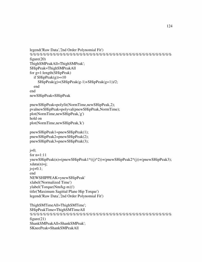
124


%%%%%%%%%%%%%%%%%%%%%%%%%%%%%%%%%%%%%%%%%%%

figure(20)

ThighSMPeakAll=ThighSMPeak';

SHipPeak=ThighSMPeakAll

for g=1:length(SHipPeak)

if SHipPeak(g)>=10

SHipPeak(g)=(SHipPeak(g-1)+SHipPeak(g+1))/2;

end

end

newSHipPeak=SHipPeak

pnewSHipPeak=polyfit(NormTime,newSHipPeak,2);

pvalnewSHipPeak=polyval(pnewSHipPeak,NormTime);

plot(NormTime,newSHipPeak,'g')

hold on

plot(NormTime,newSHipPeak,'k')

pnewSHipPeak1=pnewSHipPeak(1);



j=0;

for n=1:11

ynewSHipPeak(n)=(pnewSHipPeak1*((j)^2))+(pnewSHipPeak2*(j))+(pnewSHipPeak3);

xdata(n)=j;

j=j+0.1;

end

NEWSHIPPEAK=ynewSHipPeak'


ylabel('Torque(Nm/kg-m))')

title('Maximum Sagittal Plane Hip Torque')


ThighSMTimeAll=ThighSMTime';

SHipPeakTime=ThighSMTimeAll

%%%%%%%%%%%%%%%%%%%%%%%%%%%%%%%%%%%%%%%%%%%

figure(21)

ShankSMPeakAll=ShankSMPeak';

SKneePeak=ShankSMPeakAll

125

for g=1:length(SKneePeak)

if SKneePeak(g)>=10

SKneePeak(g)=(SKneePeak(g-1)+SKneePeak(g+1))/2;

end

end

newSKneePeak=SKneePeak

pnewSKneePeak=polyfit(NormTime,newSKneePeak,2);

pvalnewSKneePeak=polyval(pnewSKneePeak,NormTime);

plot(NormTime,newSKneePeak,'g')

hold on

plot(NormTime,newSKneePeak,'k')

pnewSKneePeak1=pnewSKneePeak(1);



j=0;

for n=1:11

ynewSKneePeak(n)=(pnewSKneePeak1*((j)^2))+(pnewSKneePeak2*(j))+(pnewSKneeP

eak3);

xdata(n)=j;

j=j+0.1;

end

NEWSKNEEPEAK=ynewSKneePeak'



title('Maximum Sagittal Plane Knee Torque')


ShankSMTimeAll=ShankSMTime';

SKneePeakTime=ShankSMTimeAll

%%%%%%%%%%%%%%%%%%%%%%%%%%%%%%%%%%%%%%%%%%%

figure(22)

FootSMPeakAll=FootSMPeak';

SAnklePeak=FootSMPeakAll

for g=1:length(SAnklePeak)

if SAnklePeak(g)>=10

SAnklePeak(g)=(SAnklePeak(g-1)+SAnklePeak(g+1))/2;

end

end

126

newSAnklePeak=SAnklePeak

pnewSAnklePeak=polyfit(NormTime,newSAnklePeak,2);

pvalnewSKneePeak=polyval(pnewSAnklePeak,NormTime);

plot(NormTime,newSAnklePeak,'g')

hold on

plot(NormTime,newSAnklePeak,'k')

pnewSAnklePeak1=pnewSAnklePeak(1);



j=0;

for n=1:11

ynewSAnklePeak(n)=(pnewSAnklePeak1*((j)^2))+(pnewSAnklePeak2*(j))+(pnewSAnk

lePeak3);

xdata(n)=j;

j=j+0.1;

end

NEWSANKLEPEAK=ynewSAnklePeak'



title('Maximum Sagittal Plane Ankle Torque')


FootSMTimeAll=FootSMTime';

SAnklePeakTime=FootSMTimeAll

%%%%%%%%%%%%%%%%%%%%%%%%%%%%%%%%%%%%%%%%%%%

figure(23)

ThighFMPeakAll=ThighFMPeak';

FHipPeak=ThighFMPeakAll

for g=1:length(FHipPeak)

if FHipPeak(g)>=10

FHipPeak(g)=(FHipPeak(g-1)+FHipPeak(g+1))/2;

end

end

newFHipPeak=FHipPeak

pnewFHipPeak=polyfit(NormTime,newFHipPeak,2);

pvalnewFHipPeak=polyval(pnewFHipPeak,NormTime);

plot(NormTime,newFHipPeak,'g')

127

hold on

plot(NormTime,newFHipPeak,'k')

pnewFHipPeak1=pnewFHipPeak(1);



j=0;

for n=1:11

ynewFHipPeak(n)=(pnewFHipPeak1*((j)^2))+(pnewFHipPeak2*(j))+(pnewFHipPeak3);

xdata(n)=j;

j=j+0.1;

end

NEWFHIPPEAK=ynewFHipPeak'



title('Maximum Frontal Plane Hip Torque')


ThighFMTimeAll=ThighFMTime';

FHipPeakTime=ThighFMTimeAll

%%%%%%%%%%%%%%%%%%%%%%%%%%%%%%%%%%%%%%%%%%%

figure(24)

ShankFMPeakAll=ShankFMPeak';

FKneePeak=ShankFMPeakAll

for g=1:length(FKneePeak)

if FKneePeak(g)>=10

FKneePeak(g)=(FKneePeak(g-1)+FKneePeak(g+1))/2;

end

end

newFKneePeak=FKneePeak

pnewFKneePeak=polyfit(NormTime,newFKneePeak,2);

pvalnewFKneePeak=polyval(pnewFKneePeak,NormTime);

plot(NormTime,newFKneePeak,'g')

hold on

plot(NormTime,newFKneePeak,'k')

pnewFKneePeak1=pnewFKneePeak(1);



128

j=0;

for n=1:11

ynewFKneePeak(n)=(pnewFKneePeak1*((j)^2))+(pnewFKneePeak2*(j))+(pnewFKneeP

eak3);

xdata(n)=j;

j=j+0.1;

end

NEWFKNEEPEAK=ynewFKneePeak'



title('Maximum Frontal Plane Knee Torque')


ShankFMTimeAll=ShankFMTime';

FKneePeakTime=ShankFMTimeAll

%%%%%%%%%%%%%%%%%%%%%%%%%%%%%%%%%%%%%%%%%%%

figure(25)

FootFMPeakAll=FootFMPeak';

FAnklePeak=FootFMPeakAll

for g=1:length(FAnklePeak)

if FAnklePeak(g)>=10

FAnklePeak(g)=(FAnklePeak(g-1)+FAnklePeak(g+1))/2;

end

end

newFAnklePeak=FAnklePeak

pnewFAnklePeak=polyfit(NormTime,newFAnklePeak,2);

pvalnewFKneePeak=polyval(pnewFAnklePeak,NormTime);

plot(NormTime,newFAnklePeak,'g')

hold on

plot(NormTime,newFAnklePeak,'k')

pnewFAnklePeak1=pnewFAnklePeak(1);



j=0;

for n=1:11

129

ynewFAnklePeak(n)=(pnewFAnklePeak1*((j)^2))+(pnewFAnklePeak2*(j))+(pnewFAnk

lePeak3);

xdata(n)=j;

j=j+0.1;

end

NEWFANKLEPEAK=ynewFAnklePeak'



title('Maximum Frontal Plane Ankle Torque')


FootFMTimeAll=FootFMTime';

FAnklePeakTime=FootFMTimeAll

%%%%%%%%%%%%%%%%%%%%%%%%%%%%%%%%%%%%%%%%%%%

figure(26)

subplot(2,1,1)

peakAccelMag=peakAccMag

for g=1:length(peakAccelMag)

if peakAccelMag(g)>=10

peakAccelMag(g)=(peakAccelMag(g-1)+peakAccelMag(g+1))/2;

end

end

newpeakAccelMag=peakAccelMag

pnewpeakAccelMag=polyfit(NormTime,newpeakAccelMag,2);

pvalnewpeakAccelMag=polyval(pnewpeakAccelMag,NormTime);

plot(NormTime,newpeakAccelMag,'g')

hold on

plot(NormTime,pvalnewpeakAccelMag,'k')

pnewpeakAccelMag1=pnewpeakAccelMag(1);



j=0;

for n=1:11

ynewpeakAccelMag(n)=(pnewpeakAccelMag1*((j)^2))+(pnewpeakAccelMag2*(j))+(pn

ewpeakAccelMag3);

xdata(n)=j;

j=j+0.1;

end

130

NEWPEAKACCELMAG=ynewpeakAccelMag'


ylabel('Area (cm2)')

title('Peak Accelerometer Magnitude Acceleration')


subplot(2,1,2)

PeakAccMagtime=peakAccMagtime

for g=1:length(PeakAccMagtime)

if PeakAccMagtime(g)<=2

PeakAccMagtime(g)=(PeakAccMagtime(g-1)+PeakAccMagtime(g+1))/2;

end

end

newPeakAccMagtime=PeakAccMagtime

pnewPeakAccMagtime=polyfit(NormTime,newPeakAccMagtime,2);

pvalnewPeakAccMagtime=polyval(pnewPeakAccMagtime,NormTime);

plot(NormTime,newPeakAccMagtime,'g')

hold on

plot(NormTime,pvalnewPeakAccMagtime,'k')

pnewPeakAccMagtime1=pnewPeakAccMagtime(1);



j=0;

for n=1:11

ynewPeakAccMagtime(n)=(pnewPeakAccMagtime1*((j)^2))+(pnewPeakAccMagtime2*

(j))+(pnewPeakAccMagtime3);

xdata(n)=j;

j=j+0.1;

end

NEWPEAKACCELMAGTIME=ynewPeakAccMagtime'



title('Time to Peak Accelerometer Magnitude Acceleration')


%%%%%%%%%%%%%%%%%%%%%%%%%%%%%%%%%%%%%%%%%%%

figure(27)

CopArea=coparea'

131

for g=1:length(CopArea)

if CopArea(g)==0

CopArea(g)=(CopArea(g-1)+CopArea(g+1))/2;

end

end

newCopArea=CopArea

pnewCopArea=polyfit(NormTime,newCopArea,2);

pvalnewCopArea=polyval(pnewCopArea,NormTime);

plot(NormTime,newCopArea,'g')

hold on

plot(NormTime,pvalnewCopArea,'k')

pnewCopArea1=pnewCopArea(1);



j=0;

for n=1:11

ynewCopArea(n)=(pnewCopArea1*((j)^2))+(pnewCopArea2*(j))+(pnewCopArea3);

xdata(n)=j;

j=j+0.1;

end

NEWCOPAREA=ynewCopArea'



title('Center of Pressure Area')


%%%%%%%%%%%%%%%%%%%%%%%%%%%%%%%%%%%%%%%%%%%

figure(28)

COPpathlength=coppathlength'

for g=1:length(COPpathlength)

if COPpathlength(g)==0

COPpathlength(g)=(COPpathlength(g-1)+COPpathlength(g+1))/2;

end

end

newCOPpathlength=COPpathlength

pnewCOPpathlength=polyfit(NormTime,newCOPpathlength,2);

pvalnewCOPpathlength=polyval(pnewCOPpathlength,NormTime);

132

plot(NormTime,newCOPpathlength,'g')

hold on

plot(NormTime,pvalnewCOPpathlength,'k')

pnewCOPpathlength1=pnewCOPpathlength(1);



j=0;

for n=1:11

ynewCOPpathlength(n)=(pnewCOPpathlength1*((j)^2))+(pnewCOPpathlength2*(j))+(p

newCOPpathlength3);

xdata(n)=j;

j=j+0.1;

end

NEWCOPPATHLENGTH=ynewCOPpathlength'


ylabel('Pathlength(cm)')

title('Center of Pressure Pathlength')


%%%%%%%%%%%%%%%%%%%%%%%%%%%%%%%%%%%%%%%%%%%

figure(29)

COPvelocity=copvelocity'

for g=1:length(COPvelocity)

if COPvelocity(g)==0

COPvelocity(g)=(COPvelocity(g-1)+COPvelocity(g+1))/2;

end

end

newCOPvelocity=COPvelocity

pnewCOPvelocity=polyfit(NormTime,newCOPvelocity,2);

pvalnewCOPvelocity=polyval(pnewCOPvelocity,NormTime);

plot(NormTime,newCOPvelocity,'g')

hold on

plot(NormTime,pvalnewCOPvelocity,'k')

pnewCOPvelocity1=pnewCOPvelocity(1);



133

j=0;

for n=1:11

ynewCOPvelocity(n)=(pnewCOPvelocity1*((j)^2))+(pnewCOPvelocity2*(j))+(pnewCO

Pvelocity3);

xdata(n)=j;

j=j+0.1;

end

NEWCOPVELOCITY=ynewCOPvelocity'


ylabel('Velocity(cm/s)')

title('Center of Pressure Velocity')


%Time to Stabilization%%%%%%%%%%%%%%%%%%%%%%%%%%%%%%%

figure(34)

plot(fPAPM(:,1),'b')

hold on

plot(fPAPM(:,jump),'k')

title('Frontal Plane AP Moment')

legend('First' ,'Last')

figure(35)

plot(fpapmout(:,1),'g')

hold on

plot(fpapmout(:,jump),'k')

figure(36)

FPapmnumber=fpapmnumber+1';

plot(FPapmnumber)

figure(37)

Xlim([0 500]);

Xl=Xlim;

Ycb=[StdFP(1) StdFP(1)];

Ycbn=[-StdFP(1) -StdFP(1)];

plot(Xl,Ycb,'g:')

hold on

plot(Xl,Ycbn,'g:')

hold on

plot(fPAPM500(:,1),'k')

figure(38)

FPAPMnumber=FPapmnumber';

for g=1:length(FPAPMnumber)

134

if FPAPMnumber(g)<=2

FPAPMnumber(g)=(FPAPMnumber(g-1)+FPAPMnumber(g+1))/2;

end

end

newFPAPMnumber=FPAPMnumber

pnewFPAPMnumber=polyfit(NormTime,newFPAPMnumber,2);

pvalnewFPAPMnumber=polyval(pnewFPAPMnumber,NormTime);

plot(NormTime,newFPAPMnumber,'g')

hold on

plot(NormTime,pvalnewFPAPMnumber,'k')

pnewFPAPMnumber1=pnewFPAPMnumber(1);



j=0;

for n=1:11

ynewFPAPMnumber(n)=(pnewFPAPMnumber1*((j)^2))+(pnewFPAPMnumber2*(j))+(

pnewFPAPMnumber3);

xdata(n)=j;

j=j+0.1;

end

NEWFPAPMNUMBER=ynewFPAPMnumber'


ylabel('Time(ms)')

title('Time to Stabilization for the Moment about Y')


135

VITA

Kristin Denise Morgan was born March 19, 1985 in Albany, New York. She graduated

from Hampton Roads Academy, Newport News, Virginia in 2003. She received her

Bachelor of Science in Biomedical Engineering from Duke University, Durham, North

Carolina in 2007 before pursuing her Masters.

THE USE OF A TRI-AXIAL ACCELEROMETER TO MEASURE …

Documents

Transcript of THE USE OF A TRI-AXIAL ACCELEROMETER TO MEASURE …