THE U.S. WINE MARKET

Hai'H "^"^

THE U.S. WINE MARKET

Raymond J. Folwell

John L. Baritelle/^''^.^ „TJ COO

-< cr m

U.S. Department of Agriculture

Economics, Statistics, and Cooperatives Service

Agricultural Economic Report No. 417

THE U.S. WINE MARKET, by Raymond J. Folwell and John L. Baritelle. Economics, Statistics, and Cooperatives Service, U.S. Department of Agriculture. Agricul- tural Economic Report No. 417.

ABSTRACT

U.S. wine buyers are Identified by major demographic characteristics, wine products purchased, and intended use of these products. Market demand functions are estimated by wine type and region. The typical wine purchasing household, according to the survey of 7,000 households on which this study is based, has higher income, fewer members, and more education than average. About half of U.S. households never buy wine, and less than 5 percent purchase more than half the wine. Two important variables influence amount of wine purchased: wine price and income level. In some markets, total industry revenues would increase if prices were raised.

Key Words: Brands, demographic characteristic, diary, demand, elastic market, grapes, inelastic market, market concentration, market penetration, panel data, total revenue, wine, winery.

Mention of brand names does not imply endorsement by the U.S. Department of Agriculture.

Washington, D.C. 20250 December 1978

CONTENTS

SUMMARY ....o iii

I. INTRQDUCTION 1

The Growth of an Industry l The Study and the Report ........................................ 3

II. A CROSS-SECTIONAL PROFILE OF THE PANEL AND REPORTED WINE PURCHASES ... 4 Representativeness of the Panel 4 Demograph i G Structure of Panel Households 11 Monthly Purchase Diary 11 Disadvantages of the Panel 11 Vol urnes of Wine Purchased 14 Purchased Wine Volume and Shipment Data ....14

III. SIGNIFICANT DEMOGRAPHIC CHARACTERISTICS OF THE WINE PtiRCHASERS 18

Demographics of Purchasing and Nonpurchasing Households , 18 Types of Wine Purchased 20 Household Demographics by Type of Wine Purchased 22

IV. FACTORS IN WINE PURCHASING 25 Sex of Purchaser 25 Age of Purchaser ,27 Occasion for Purchase , 28 Probable Consumers of Wine Purchases 30 PI ace of Purchase 32

V. MARKET CONCENTRATION, PENETRATION, MARKET SHARES, AVERAGE PRICES, AND BRAND PREFERENCES 34

Market Concentrati on and Penetration of Wi ne Sal es 34 National Market Shares ......... ...38 Regional Market Shares and Average Prices 41 Brand Preferences in Wine Purchases 42

VI. THE CHANGING U.S. WINE MARKET 46 Wine Drinkers and Nondrinkers . ^ 46 Factors Leadi ng to Wi ne Buyi ng 53 1975 Wi ne Purchases Compared with EarTier Buying 53

VII. MARKET DEMAND FUNCTIONS FOR WINE IN THE UNITED STATES ....56 Data and Methods ... 57 Table Wines 61 Dessert Wines 69 Flavored Wines 71 Sparkl ing Wines 75 Vermouth 78 Brandy ^ 80

REFERENCES 82 APPENDIX 85

n

SUMMARY

This report investigates the market structure of the U.S. wine industry, and explores who buys wine in the United States and why. It is based on a survey panel of about 7,000 households, who reported their monthly wine purchases from February 1975 through January 1976. Panel members also completed a questionnaire on their attitudes, factors leading to wine purchases, and what influenced their use of wine products. Wine products considered in this report include varietal table>.nonvarietal table, dessert, "sparkling, and flavored wines, as well as vermouth and brandy.

Households that bought table wine (varietal or nonvarietal) had more education and higher household incomes than the average household that bought other types of wine. The wives in these households were slightly older and the families slightly smaller than for those households that bought other types of wine. In contrast, the households purchasing dessert and flavored wines tended to be slightly less educated, with smaller household incomes and larger families.

To investigate the concentration of wine purchases, the households purchasing wines were arrayed as to the total quantity of wine purchased, and then divided into ten equal deciles. This revealed that the first decile of households purchasing wine accounted for 54.4 percent of all the wine bought by the households during the survey period. This decile accounted for only 3.5 percent of all the households on the panel. The two largest deciles bought two- thirds of the wine.

The demographics of the wine purchasing households by deciles showed that the households that bought the largest volumes of wine had the highest incomes, a highly educated male head, and smaller families, and were slightly further along in their life cycle as indicated by the age of the wife.

Households that bought the most wine paid lower average prices, gaining economies of size in their buying.

Gallo accounted for 32.9 percent of the wine market, and United Vintners for 12.9 percent. The four largest wine companies accounted for 54.1 percent of all wine purchases. The 8 largest companies accounted for 64.5 percent while the 10 largest wine companies accounted for 66.7 percent of the wine purchases reported by the panel.

The market shares held by the companies on a national basis were not necessarily reflected in their regional market shares. Many wineries service different segments of the U.S. wine markets with different products. In addition to the different relative market shares in various regions, the average prices paid per ounce for the various wine types produced by the largest companies in the United States differed among the regions. These differences in average prices are partly caused by the varying taxes imposed by States.

Brand preferences were explored. For varietal table wines, strong brand loyalty was shown for United Vintners, Mögen David, and Franzia Brothers.

iii

strong brand preference was assumed when a household bought at least 50 percent of a given wine product from one firm. Brand loyalty for nonvarietal table wines was weaker than that for varietal table wines, with households expressing brand loyalty only to Gallo and Canandaigua nonvarietal table wine. Brand loyalty or preference was found for dessert wines produced by Gallo, Guild, and Taylor. In the sparkling wine category, brand preferences were found for Gallo, Franzia, and Guild. Only the Gallo and Mögen David flavored wines appeared to have strong brand preferences.

While there was some degree of brand preference for all wine types, the panel of households did not show strong brand preference for all wines produced by a single company. Although there was substitution of wine purchases by the households on the panel, each company appears to serve, to some extent, unique segments of the U.S. wine market.

Over 30 percent of the panel households never drink wine. Almost 40 percent of those never drinking wine refrained because of personal or religious beliefs. This was especially true in the South. However, many nonconsumers appeared to lack enough knowledge and confidence to make their first purchase. This seems to be confirmed by the importance of brand name and advice of friends reported by the purchasing households. Sixteen percent of the panel households drank less wine during the study year than the year before.

Demand functions were estimated for each of the major wine types considered. The resulting functions were used to analyze the implications of pricing policies at the industry level, as well as to ascertain the impact on the demand for various wine types from changes in the explanatory variables. Degrees of price elasticity varied by wine type and by region. In most cases where income was statistically significant, increased income was associated with an increased demand for wine. In yery few cases was the price of a substitute wine type statistically significant in explaining the variation in the quantity demanded. Usually, only price and income were the explanatory variables affecting demand.

TV

THE U.S. WINE MARKET

by

Raymond J. Folwell

and

John L. Baritelle

I. INTRODUCTION

The U.S. wine industry has shown extraordinary growth in the I960's and 1970*s, yet little has been reported about the U.S. wine market. Who buys wine in the United States? When and for what occasions is it bought? What are the characteristics of the wine market and wine marketing in the United States?

Before this study was initiated, there was no adequate data set relating to the U.S. wine market. The only market information available to the U.S. wine industry was shipment data or volumes entering distribution channels based on tax withdrawals, inventory data, and number of wineries. But relying on this type of secondary data, it was impossible to say precisely who purchases wines and why, or to answer various marketing questions ranging from physical distribution patterns to pricing problems. The information in this report aims to answer these questions.

The Growth of an Industry

The wine industry is unparalleled in the American industrial economy in terms of its growth in sales and its market organization. It is unique in terms of the number and sizes of firms, the concentration of the industry on the East and West Coasts, the large number of different types and variations in wine products produced, and the unprecedented market growth rate some of its wine products have enjoyed (8, 19). 1/

Raymond J. Folwell is Associate Professor of Agricultural Ecofiomics, Washing- ton State University, Pullman, Wash. John L. Baritelle is an Agricultural Economist with the Economics, Statistics, and Cooperatives Service, U.S. Depart- ment of Agriculture, Washington, D.C. y Underlined numbers in parentheses refer to citations listed on pages 82-84

of"this report.

The wine industry in the United States, which started for a second time after Prohibition, has been dominated byvfamily-owned companies. The itidustry did not grow much in size until the I960's. In the late 1960's the U.S. wine market boomed and sales rose at unprecedented annual rates—as high as 14 percent in some years (39). Witt) the wine boom, sales grew at fantastic rates, and some wine companies were bought, merged, or consolidated with conglomerate eorporations. Other wine companies remained as family owned or controlled enterprises.

This growth in sales is quantified by the following volumes of wine that entered distribution channels in the United States (39):

Total

Year

Type of wine 1956 1960 1964 1968

Gallons

1972 1976

Per capita: 2/

Table wine U.S. Imported Total

Sparkling Dessert and other 1/

All wine

.24

.02

.26

.02

.61

.89

26 03 29

.32

.05

.37

.41

.06

.47

.65

.18 ,83

.85

.23 T.Ö8

02 .03 .06 .11 .10

59 .57 .53 .68 .57

91 .97 1

1,000 igäl Ions

.07 1.62 1.75

Table wine U.S. Imported Total

40.820 3,834

44,655

47,467 5,603

53,071

61,698 8,651

70,349

82,791 13,041 95,831

136,340 37,478

173,818

181,982 49,412

231,394

Sparkling Dessert and other 3/

2,779

102,605

4,321

105,960

6,543

108,733

12,513

105,314

22,299

140,864

21,764

123,145

All wine 150,039 163,352 185,625 213,658 336,981 376,303

3/ Computed on a residual basis by subtracting table and sparkling wine gallonage froin total wine gallonage.

In terras of 4-year growth rates, the increases in the amount of wine entering distribution channels were 8.9 percent between 1956 and 1960, 13.6 percent between 1960 and 1964, 15.1 percent between 1964 and 1968, 57.7 percent between 1968 and 1972, and 11.7 percent between 1972 and 1976. The growth rates as shown by each of the changes in wine shipments over 4-y^ar periods indicate the rapid increases in sales and then the leveling off that has characterized wine sales in more recent years. The growth rates over 4-year periods were modest until the late 1960*s and early 1970's. In those years a wine boom occurred and the industry responded with new grape acreage and wineries. Not only did the traditional wine producing areas in California and New York expand, but new entities in Washington, Oregon, and other States began to appear. The industry was enjoying a period of market growth that was beyond its expectations.

Despite the wine boom and the initial growth of numerous new commercial wine industries in various States, California still accounted for 86 percent of gross U.S. wine production in 1975. New York was the second most important State in terms of gross wine production, accounting for 10 percent of the 1975 volume. The wine industry continues to be concentrated in terms of its location pattern.

For the most part, the concentration of wine production has historically centered around the major areas of grape production, California and New York. The wine industry is this Nation's leading market for crapes, which are one of the major fruit crops of the Uhited States, frequently*surpassing apples and oranges in value of production. In 1975, the year of the study, the value of production for grapes was $618] million and in 1977 the value of production was $776.1 million. Since 1970 mojre than 60 percent of the grape crop has been crushed for wine and juice production. Wine and its major ingredient, grapes, are an important part of American agriculture.

The Study and the Report

The data used in this analysis-were gathered from a panel of households in the United States, consisting of about 7,000 households at any one time between February 1975 and January 1976. Members of this panel reported their monthly wine purchases that were related to household use of the wine. They did not include wines purchased for consumption away from a household setting, such as in a restaurant. All of the major demographic features, such as age, sex, incoïTfâ, occupation, education, race, marital status, and region of the country, were also available, so they could be cross tabulated with each household's purchasing patterns.

This report gives insights into consumer buying attitudes and patterns. The information includes:

1. An analysis of the demographic characteristics of wine purchasing households by type of wine purchased,

2. The proportion of the total population in a given region that buys wines (degree of market penetration),

3. The estimated market shares held by the largest wine companies,

3

4. The average prices paid for various types of wine in the United States, by wine type and individual company,

5. The degree of brand preference in wine purchasing,

6. The changing wine purchasing patterns in the United States,

7. Estimated statistical market demand functions for various wines and pricing policy implications, and

8. General facts about wine buying and motivation for purchasing wines.

This report is intended for an audience consisting of the wine industry, researchers, and various other industries that serve the wine industry such as manufacturers of packaging materials and advertising firms. Some of the material is analyzed in such a fashion that an individual not familiar with economics and statistics will have difficulty in fully understanding the statistical analyses. However, an effort is made to explain the implications of the results to those without a full understanding of the statistical methods employed.

II. A CROSS-SECTIONAL PROFILE OF THE PANEL AND REPORTED WINE PURCHASES

This chapter presents an overview of the household panel that reported their wine purchases via a monthly diary. The panel of households is described in terms of its selection and what the panel represents in terms of all U.S. households. The monthly diary and the limitations of market information generated in this manner are discussed. Finally, the reported wine purchases made by the panel member households are compared with the volume of wine entering distribution channels in the United States during the time period.

Representativeness gf the Panel

The panel of households used in this wine research effort was maintained by National Purchase Diary (NPD) of New York City. The household panel was maintained solely for the purpose of collecting information about the purchase of various goods, principally food and grocery items. The households were selected by NPD to represent a cross section of all households in the United States. The household panel member responding was the female head of household or the wife. The households were rewarded through a gift from NPD for reporting the purchase{s) of various items in the monthly diaries.

The household panel consisted of 11,522 households from February 1975 through January 1976. Not all of the households were on the panel for the entire period, and an average of about 7,000 households participated at any one time. This report is based on all the households, regardless of the length of time they served on the panel.

The households or panelists are those defined by the Census Bureau of the U.S. Department of Commerce (38). A household as used herein is a group of two or more persons residing together in the same household.

The panel of households was not a probability sample. The households were recruited by a telephone survey to serve on the panel. Attempts were made to make the panel representative of U.S. households according to census region, age, income, and education. The households were selected and/or replaced according to household size, income, and education so that the panel would represent U.S. households as defined by the Census Bureau. Figure 1 delineates the census regions used in this study.

Because the panel was not a probability sample, because single member households were not included on the panel, and because there was some turnover in households on the panel, the panel did not match in all instances the estimated percentage distributions of households according to major census household demographics. The information in the remainder of this section provides a basis for establishing how closely the panel of households represented all U.S. households.

Age

Table 1 presents the percent distribution by age of the heads of households for the households on the panel and for all households in the United States. The table shows that the panel had a greater proportion of households in the age group 25 to 44 years. The panel had proportionally fewer male heads of households in the age groups 14 to 24 and 65 years and over than did the United States as a whole.

On a national basis, the panel truly represented the households in the middle-aged group, those with a male head of household 45 to 65 years old. The percent distributions on the panel and in the United States were almost equal. The panel overrepresented the households whose female head was less than 65 years of age. It underrepresented the households whose female head was 65 years or older. In the 14 to 24 years of age category, the panel underrepresented U.S. households on the basis of the age of the male head, and overrepresented on the basis of the female head.

The aggregate representation at the national level of all households on the panel by aqe of male head of household was also true on a regional 4/ basis (table 1). As an example, the age group of 45 to 64 years of age for the male head of the household, the panel contained 36.4 percent of the households

4/ The smallest areas or regions with about the same distribution by ranges of ages were the four major Census regions of the United States. Therefore, the regions shown in fig. T were consolidated into the larger Census regions as follows: (1) the Northeast region consists of the New England and Middle Atlan- tic regions; (2) the North Central region consists of the East and West North Central regions; (3) the South region consists of the South Atlantic, East South Central, and West South Central regions; and (4) the West region consists of the Mountain and Pacific regions..

Figure 1. U.S. Census regions usçd as market regions in this study

East North

a»

A—

/Móunteinr ^^

' \>? '""Y" Middle J^' Atlantic ^^ (2) /

EastSouth \ \ CenM \

AP K._ C h >p Pacific 1

(9) 1 .^ North \ y \ ^ Central \——1

Í \ \ 1 ^*' ^ \

/

\^ L, ^1 South Atianttc

West Stouth Central I J (5)

1

Table 1. Age of male and female heads of household, panel households and all U.S. households

Male Female

Region Total 14-24 years

25-44 years

45-64 years

65 years and over Total

14-24 years

25-44 years

45-64 years

65 years and over

100 4.67 49.09 36.37

— Panel

9.87

of households Percent

100 United States 8.90 50.64 34.64 5.82

Northeast North Central

100 100

4.94 5.15

52.62 49.45

34.54 35.32

7.09 10.08

100 100

9.65 9.17

56.51 49.81

29.03 35.16

4.81 5.86

-j South West

100 100

4.57 3.59

47.31 46.22

37.86 38.44

10.26 11.75

- All U.S

15.35

100 100

. households Percent

100

8.60 7.82

a/

3.36

48.38 47.53

22.91

37.14 37.54

32.99

5.88 7.11

United States 100 7.16 40.98 36.51 40.74


100 100

5.24 6.75

39.77 40.19

38.77 37.83

16.22 15.23

100 100

2.47 3.47

21.50 21.75

32.80 32.14

43.23 42.64

South West

100 100

8.49 7.88

41.78 42.34

34.27 35.60

15.46 14.18

100 100

3.30 4.42

22.02 27.86

34.13 32.41

40.55 35.31

a/ U.S. Dept. Commerce, Bur. of the Census, Population Cnaracteristies Series P-20, No. 271, issuea October 1974.

in this age group on a national basis, while the estiraated number of households in such an age group by the Census Bureau was 36.5 percent in 1974. Regionally, the panel underrep^resented or overrepresented the number of households in the 45 to 64 years of age group by only a few percentage points. Based upon the percentage distribution by age, the panel of households is very representative of middle-aged households which comprise one of the greatest concentrations of the entire population.

Education

The percentage distribution by education of the head of the panel households on national and regional bases are presented in table 2. Table 2 also shows the percent distribution by education of the heads of all U.S. households in 1973. The percentage distributions by education level on a regional basis for all U.S. households were not available at the time this research was done.

In aggregate, the panel overrepresented households in which the male head had at least some college education and underrepresented households whose head had a high school education or less. The percent of households on the panel whose head had some high school or a high school education was closer to the percent of such households throughout the United States than it was for those with only an elementary school education. The panel was lacking in terms of representing those households whose head had only an elementary education.

On a regional basis the representation of the panel in terms of education of the head of the household was the same as on a national basis. The households with less than a high school education level tended to be underrepresented, while households with more education tended to be overrepresented.

Income

To compare the average household incomes of the panel households to the average incomes of all U.S. households on a regional basis, regions were consolidated as shown in figure 1 into the four regions described in footnote 4. Table 3 shows that the panel was representative of households with annual money incomes between $5,Q00 and $9,999. The panel underrepresented households in the United States with annual incomes of less than $5,000 and overrepresented households with incomes exceeding $10,000 per year.

Regionally, the panel of households usually closely represents the percent* age of households in each income category found by the national census. The few exceptions were within a few percentage points of exact representation.

Overall, the panel overrepresented middle-aged households with at least some college education and annual incomes in excess of $10,000. Inferences from the informat i on presented in this report must be made keeping in mind how well the panel represented U.S. households. As will be shown later, most wine buying households in the United States tend to be in those categories that are overrepresented on the panel.

Table 2. Education level of head of household, panel households and all U.S. households

<^

Region

N. England Mid Atlantic E. N. Central

W. N. Central S. Atlantic E. S. Central

W/ S. Central Mountain Pacific

All panel households

All U.S. households a/ 23.4

ETementary Some High School Some College School High School Graduate Goll lege Graduate Tota

Percent 5.94 15. ,35 30, ,03 21. .45 27, ,23 100 3.87 13. ,34 30, .75 21. ,69 30. ,35 100 5.81 12. ,79 32, .36 24. ,12 24.92 100

12.72 14, .14 31, .25 19. ,08 22, .81 100 5.93 11, .67 25, .10 25, .81 31, .49 100 9.88 16, .26 24, .32 23, ,10 26, .44 100

6.14 13.28 24, .33 24.44 31, .81 100 6.80 9, .90 24, .54 24.95 33, .81 100 3.46 9, •27 21, .46 35, .84 29, .97 100

6.10 12, .68 27, .95 24, ,79 28, .48' 100

23.4 15, .7 32, .7 13, .1 15, .1 100

a/ U.S. Dept. Commerce, Bur. of the Census, Consumer Information Series P-60, No. 96, issued August 1974. Data is for 1973.

Table 3. Distribution of all panel households by annual money income

Region


South West

All regions


South West

United States

Under $3,000

1.15 1.51

2.04 1.60

1.59

3.2 3.9

8.2 4.7

5.31

$3,000 to

$4,999

4.13 3.98

4.45 4.02

4.16

7.3 6.2

9.8 7.2

7.80

$5,000 to

$6,999

5.99 6.75

7.07 5.51

6.45

7.6 7.9

10.3 9.4

8.89

$7,000 to

$9,999

$10,000 to

$11,999

Panel of households Percent

11.63 14.21 11.56 13.89

12.84 14.73

12.47

13.45 12.36

13.58

All U.S. households a/ Percent

13.1 12.7

15.2 14.1

13.83

10.0 10.2

10.7 9.6

10.23

$12,000 to

$14,999

20.70 19.16

19.57 18.58

19.55

14.5 15.5

13.4 12.9

14.14

$15,000 or

more

42.19 43.15

40.58 43.20

42.20

44.30 43.6

32.4 42.1

39.80

Total

100 100

TOO 100

100

100 100

TOO 100

100

a/ U.S. Dept. Commerce, Bur. of the Census, Consumer Income Series P-60, No. 101, issued January 1976.

Demographic Structure of Panel Households

The complete demographic structure of each household on the panel was made available so that purchase information could be cross tabulated with the demographic data. The kind of demographics available on each household is listed in table 4. The subclasses of a demographic feature and the codes used in analyzing the data are also shown.

Previous analysis showed that the major demographic characteristics that segregate wine-purchasing from nonpurchasing households are the region of the country, age of wife, size of family, education level of the male head, and annual household income (30, 34). Thus, for brevity, the other demographic items shown in table 4 were not used in this analysis.

Monthly Purchase Diary

Each panel household was supplied with a monthly diary in which it recorded all wine purchases and other information concerning each wine purchase. Figure 2 shows a completed diary. Each diary for each household was identified by the household identification number (261 7512 in fig. 2). It was then possible to take the purchase information from the monthly diaries and combine it with the complete demographic data for each individual household. The purchase data for each household were so coded that all cross-tabulations were possible among the purchase data and the household demographics as shown in table 4.

Wine types were identified in the coding of the purchase data for the entire 12 months of the panel. A code for each of the largest 13 wine companies in the United States was also used during the last 6 months of the study. Thus, the wine type could be identified by individual company in analyzing the purchase data. The wines were identified by company for only 6 months of the study: August 1975 through January 1976.

Disadvantages of the Panel

The panel represented households, not the total population. According to U.S. Census data (1973), the country contains about 54 million families representing 90 percent of the population (38). Conspicuously missing from the panel were young persons not living in family units. Young single persons' extreme mobility makes it hard and expensive to keep them on consumer diary panels.

Another limitation was the exclusion from the diary of wines purchased while dining out. Another general problem arises from the fact that the diary initially advertises the product under study. Panel members can be expected to buy more of the product than normal during the first month the product is in the diary.

A problem that occurs with diary-type mail panels is the consumer's interpretation of what he has bought. Occasionally what is written on the diary is incorrect, incomplete, or uninterpretable. When this happens, the person transcribing the purchase data must objectively try to interpret the diary

11

Sample diary of reported wine purchased by panel household

IJEC. 2.4,1 " ̂ 5\z

Extra space page 1. Free Giftsand Samples, inside front cover. WINE DIARY TIPS: Include all wine purchased for consumption at home or outside the home: Also include wine Douqht to give as a gift. Write in all types such as TABLE WINES, DESSERT WINES (like Sherry, Port, etc.) SPARKLING (like Champagne, Cold Duck, etc.), FLAVORED (like Apple, Berry). VERMOUTH, BRANDY or COGNAC. DO NOT INCLUDE wine consumed at a restaurant.

Date of mnth

purchase was

made

Write in

BRAND NAME as shown on label

HOW MANY

of each kind did youbuy?

1 HOW MUCH DID YOU PAY? 1 WHERE DID YOU PURCHASE? WEIGHT

SHOWN ON LABEL

Write in size such as 10 oz, 12 0Z..16

QZ.. qt. Size etc

FULL DESCRIPTION

OF WINE

1 FLAVOR

Write in flavor

such as: Apple Wine.

Apricot Brandy,

etc,

COPY FROM LABEL

COLOR OF

WINE

Check (/) One

PLACE Of ORIGIN

Check (/) One

WHO PUR-

CHASED

OCCASION FOR PURCHASE Check (/) as many as apply

WHO WILL

TOTAL CASH PAID

Don't Include taxes

Was this a special price or offer?

NAME OF STORE

(or company if purchased

from door-to-door or home delivery

salesperson)

KINO OF STORE Check (*-') or write in.

PROBABLY DRINK SOME?

Check {y^ as many as apply

1 For Use At Home

«

Write in such as; "White Table Wme.- "American Rieslmg,"

"Sparkling Burgundy." etc

COPY FROM LABEL

IF NO.

Check here

.fTts.aescriDe kind such as Store sale, cents-off; coupon,

gift on or In package, etc. How much savings in total? £

1 2

i Other-

Describe

DOMESTIC IMPORTED

1 t Î WINES

— 1

Write in number of

bottles.

containers'

'E

1 s: 1 1 1 1 1 C3

d;\

Age and Sex 1

E

1

"S 1 1 f

1 1 1 3? $ < DESCRIBE SPECIAL PRICE OR OFFER

Total (Off

Ï

'' s ^ 34 Klo(piíVxTkí¡4 ..\ -L m V^ Copi^U TU ^H^ tcm«?HAM)iiAt. EiffctoC Á " ̂ _

1 ~ ^ M E —' — le — ■M I - • 1 r 1—1 p_»

- ^~ ■,..' ' • ■"^ — — — JL-

, _ ~~ ~ "~ _ - ^" — ~ \—

~ — ~ — ^

'!''":;'' r _ — — ^ — ^ 1 — -i -.^ ... _ 1 Z ~

Figure 2

Table 4. Demographic features and subclasses available monthly for each panel household

AGE. FEMALE HEAD EMPLOYMENT STATUS, FEMALE HEAD

1 - Under 25 1 - Employed 2 - 25-34 2 - Not employed 3 - 35-44 4 - 45-54 OCCUPATION, MALE HEAD 5 - 55-64 6 - 65 & over 1 - Professional

2 - Proprietors, managers , officials AGE, MALE HEAD 3 - Clerical

4 - Sales 1 - Under 25 5 - Craftsmen/foremen (sk illed) 2 - 25-34 6 - Operative (semiskilled) 3 - 35-44 7 - Private household worker 4 - 45-54 8 - Service workers 5 - 55-64 9 - Farm owners, managers 6 - 65 & over 10 - Farm foremen, laborers

11 - Laborers AGE & PRESENCE OF CHILDREN 12 - Retired, unemployed, military, student

1 - Under 6 only INCOME 2 - 6-12 only 3 - 13-17 only 1 - Under $3,000 7 - $10,000-10,999 4 - Under 6 & 6-12 2 - $3,000-4,999 8 - $11,000-11,999 5 - Under 6 & 13-17 3 - $5,000-6,999 9 - $12,000-12,999 6 - 6-12 & 13-17 4 - $7,000-7,999 10 - $13,000-14,999 7 - All three age groups 5 - $8,000-8,999 11 - $15,000-19,999 8 - No children under 18 6 - $9,000-9,999 12 - $20,000 & over

MARITAL STATUS EDUCATION, FEMALE HEAD

1 - Married 1 - Grade school 2 - Single 2 - Some high school 3 - Widowed 3 - Graduated high school 4 - Separated or divorced 4 - Some college

5 - Graduated college or more EDUCATION, MALE HEAD

YEAR OF BIRTH 1 - Grade school 2 - Some high school Actual 3 - Graduated high school Last 2 digits 4 - Some college 5 - Graduated college or more RELATIONSHIP

RACE 1 - Son 2 - Daughter

1 - White 3 - Other male relation 2 - Black 4 - Other female relatior 1 3 - Oriental 5 - Other male 4 - Other 6 - Other female

FAMILY SIZE CENSUS DIVISION

1 - Single member (certain 7 - Seven member 1 - New England 6 - East South Central supplements only) 8 - Eight member 2 - Middle Atlantic 7 - West South Central

2 - Two member 9 - Nine member 3 - East North Central 8 - Mountain 3 - Three member lo- Ten member 4 - West North Central 9 - Pacific 4 - Four member ll - Eleven member 5 - South Atlantic 5 - Five member 12 - Twelve member 6 - Six member or more MARKET SIZE

MONTH OF BIRTH 1 - 50,000-99,000 2 - 100,000-249,000

1 - January 7 - July 3 - 250,000-499,000 2 - February 8 - August 4 - 500,000-999,999 3 - March 9 - September 5 - 1,000,000-2,499,999 4 - April 10 - October 6 - 2,500,000 & over 5 - May 11 - November 9 - Non-SMSA 6 - June 12 - December

13

infomâtion. Typically, 20 to 40 householct diaries needed interpretation each month. Approximately half of these diaries were salvaged.

Volumes of Wine Purchased

The volumes of wine reported purchased by the panel of households from Feb- ruary 1975 through January 1976 are shown in table 5. The total quantity of wine purchased by the households was 1,224,715.7 ounces during the 12 months. This amounts to 9,568.1 gallons. Households reported 21,219 purchases, an average of 57.7 ounces or 0,45 gallons per purchase.

The volumes bought were classified by origin (domestic or imported), and by wine type such as varietal table wine, etc. Table wines are naturally fermented and contain 14 percent or less alcohoT by volume. Varietal table wines are those that contain at least 51 percent of the juice from a given variety of grapes and are marketed under that variety name. Nonvarietal table wines or generic table wines are blends of various varieties of grapes, Nonvarietal table wines are usually named after a famous wine-producing region in the world such as Burgundy, Rhine, etc. Dessert wines are produced by the addition of wine spirits and as a rule contain 15 to 20 percent alcohol by volume. They include sherry and port. Spar^kling wines have more than 0.256 grams of carbon dioxide per milliliter. The principal sparkling wines are champagne^ burgundy, and cold duck. Flavored wines are defined as those produced primarily from fruits other than grapes and have the dominant flavor of that fruit, e.g., apple, berry, or citrus. Vermouth is a type of aperitif wine made from grapes but having the ^'tas te and characteristics attributed to vermouth'* because it is flavored with herbs. Brandy is a grape product that has been distilled to concentrate the alcohol to a higher percentage than occurs in the wine naturally.

Nonvarietal table wines dominated the wine purchases reported by the panel houselîolds {table 5). These wines accounted for 67.2 percent of the total volume purehased by the households. Varietal table wines, dessert wines, and flavored wines were bought in about the same quantities (9 percent of each) by panel households. The types shifted in relative Importance when analyzed on a domestic and imported basis.

The panel bought relatively little imported table wine, 11.6 percent of the total volume of wine purchased.

Sparkling wines were only 3.6 percent of the total volume purchased. Ver- mouth and brandy were the least important, accounting for 1.6 and 0.3 percent, respectively, of the total volumes bought.

Purchased Wine Vgl me and Shipment Data

The volume of wines purchased by the households (table 5) is compared to the volume of wines that was shipped or entered distribution channels in the United States (table 6). This information adds to the foundation from which any conclusions and inferences are drawn from this report. To allow the wine to flow through the distribution channels and reach retail shelves, a time lapse of 1 month was used in the comparison. Thus the shipment data for two 12-month

14

Table 5 . Quantity of wine types purchased

Wine Ounces Percentage type purchased of total

DOMESTIC

Varietal table 114,778.9 9.4 Nonvarietal table 711,510.8 58.1 Dessert 107,728.8 8.8 Sparkling 42,313.3 3.5 Flavored 89,017.4 7.3 Vermouth 13,036.8 1.1 Brandy 2,646.2 .2 Other 1,690.6 .1

Total domestic 1,082,722.8 88.4

IMPORTED

Varietal table 1,262.8 .1 Nonvarietal table 111,718.84 9.1 Dessert 4,200.999 .3 Sparkling 1,270.6 .1 Flavored 15,825.787 1.3 Vermouth 6,660.692 .5 Brandy 641.8 .1 Other 411.6 .03

Total imported 141,993.10 11.6

ALL WINE

Varietal table 116,041.7 9.5 Nonvarietal table 823,229.64 67.2 Dessert 111,929.79 9.1 Sparkling 43,583.9 3.6 Flavored 104,843.18 8.6 Vermouth 19,697.492 1.6 Brandy 3,288.0 .3 Other 2,102.2 .2

■Grand total 1,224,715.7

(9,568.1 gal)

100.0

15

Table 6. Volumes and percentage distributions of wine entering distribution channels and reported purchases by household panel

Shipments - wine Reported entering distribution household panel

Wine origin channels purchases

and type 1975 1976

DOMESTIC - - - 1,000 gallons - - - Gallons

Table 173,511 181,982 6,455.4 Dessert 64,650 57,998 841.6 Vermouth 5,272 5,220 101.8 Sparkling 18,435 19,205 330.6 Flavored a/ 56,842 52,979 695.5 Brandy b/ 10,433 10,730 20.7 Other c/ — 13.2

Total 329,143 328,114 8,458.8

Shi pments - wine Reported entering distribution household panel

channel s purchases

1975 1976

- — Percent - - -

52.7 55.5 76.3 19.6 17.7 9.9 1.6 1.6 1.2 5.6 5.9 3.9 17.3 16.1 8.2 3.2 3.3 0.2 — _— 0.2

100.0 100.0 100.0

IMPORTED

Table 40,524 49,412 Dessert 2,589 2,931 Vermouth 4,278 4,017 Sparkling 1,928 2,559 Flavored a/ — — Brandy b/ 2,562 3,396 Other c/ — —

Total 51,881 62,314

2.7 32.8 52.0 9.9

123.6 5.0 3.2

1,109.2

78.1 5.0 8.2 3.7

4.9

100.0

79.3 4.7 6.4 4.1

5.4

100.0

79.6 3.0 4.7 0.9 11.1 0.5 0.3

100.0

ALL WINE

Table 214,035 231,394 Dessert 67,239 60,929 Vermouth 9,551 9,237 Sparkling 20,363 21,764 Flavored a/ — — Brandy b/ 12,995 14,126 Other c/ 56,842 52,979

Total 381,024 390,429

7,338.1 874.5 153.9 340.5 819.1 25.7 16.4

9,568.1

56.2 17.6 2.5 5.3

3.4 14.9

100.0

59.3 15.6 2.4 5.6

3.6 13.6

100.0

76.7 9.1 1.6 3.6 8.6 0.3 0.2

100.0

a/ Other special natural wine in Wine Institute reports. F/ Proof gallonSp £/ Not reported in shipment data. Source: Wine Institute Statistical Reports, San Francisco,

periods of January 1975 through December 1975 and January 1976 through December 1976 were compared to the diary purchase data of February 1975 through January 1976.

To compare the reported volumes of wine purchased with the shipment data, it was necessary to make certain aggregations. The shipment data from a secondary source were first secured from Government reports on tax withdrawals (39). The taxation of wine is based primarily upon alcohol content, and thus the shipment data do not correspond with the wine types described in the previous section. The differences in the definitions of wine types for the shipment data and household panel data are noted below:

Wine type

Table

Dessert

Vermouth

Shipment data

All wine under 14% alcohol that is not flavored (grape or nongrape)

Wine 14-21% alcohol that not flavored (grape or nongrape)

Aperitif wine made from grapes and flavored with herbs

IS

Household panel data

All grape varietal and nonvarietal wines less than 14% alcohol

Wine 14-21% alcohol that may or may not be flavored

Aperitif wine made from grapes and flavored with herbs

Sparkling

Flavored

Wine containing more than 0.256 grams of carbon dioxide per mi 11 i liter and not flavored

Wine under 14% alcohol that has been flavored

Other Wines not defined above

Wine containing more than 0.256 grams of carbon dioxide per milliliter and may or may not be flavored

Wine under 14% alcohol that may or may not have been flavored but is not a grape base varietal or nonvarietal (generic) table wine

Wines not defined above

The shipment data are based on the alcohol content of the wine and the base from which the wine is made» grape or other fruit. The household panel purchase data are grouped into wine types for purposes of marketing research and agree more closely with terms used in wine marketing and merchandising.

Table 6 presents the shipment data and purchase data from the household panel in gallons and percent distribution by wine types. The differences in the percentages of wine types shipped and reported purchased by the panel of households are due to three main factors. The first factor is the differences in the definitions of the various wine types. The second is the degree to which the

17

panel overrepresents Gertain types of households in the United States. Third, inventory adjustments could contribute to the differences.

The most notable difference between the household purchase and shipment data occurs in the table wine category. About three-fourths of the total volume of wine bought by the panel was table wine. During a similar period, according to shipment data in table 6, 56 percent and 59 pereent of the total volume entering dis^tribution charinels was table wine. The tat)Te wine purchased by panel members comes at the expense of the dessert, sparkTing, and flavored wines. The panel of households bought less of these wine types than appears in the shipment da ta.

The differences between shipment data and household data might be explained by definition differences and inventory changes. However, the differences most likely accurred because the composition of the panel overstates table wine consumption. The underrepresentation of older househoT<ls (housewife over 54 years of age) leads to an understatement of sparkling and dessert wine consumption relative to table wine (8, 23, 29, 31). The understatement of flavored wine consumption is likely due to the lack of young singles and underrepresentation of low-income househoTds with a housewife under 25 years old.

III. SIGNIFICANT DEMOGRAPHIC CHARACTERISTICS OF THE WINE PURCHASERS

This chapter deals with the important demographic features that identify households buying different types of wine. Wine-purchasing households are noted on the basis of family size, age of the wife, age of male head, age of purchaser, size of family or household, and education level of the male head. Also, household incomes of wine buying and nonbuying households are compared. The same fTOUsehold demographic characteristics are used to identify households that buy various wine types in different regions of the country.

The focus of this chapter is on domestic wines. Tabular summaries of the same information on households buying imported wines is in a&pendix tables S throjjgh 15.

Demographics of Purchasing and Nonpurchasing Households

Only the most important demographics identified in previous work were used to isolate and describe wine purchasing and nonpurchasing households (30,34). These demographics were the age of the wife or female head of the househoTd, age of the male head of household, education level of the male head of the household, size of family or household, and household income. The computed mean values of these major demographics for the purchasing and nonpurchasing households are in table 7.

The major demographics of the purchasing and nonpurchasing households were compared^on a regional and on a nationaT basis. On the average, the wife and male head of household tended tobe slightly older in the purchasing households than in the nonpurchasing households. The only significant differences at the .05 probability level between the purchasing and nonpurchasing households were

18

Table 7. Demographics of wine purchasing and nonpurchasing households, by region

Region

Age of wife

Age of male head

Size of family

Nonpurchasing

Education of male

head

households

Household income Number of

households

Years Number Code a/ Dollars Number

N England Mid Atlantic E N Central

36 34 36

39 37 39

3.5 3.7* 3.6

3.3* 3.4* 3.3*

11,982* 13,849* 14,184*

353 1,211 1,536

W N Central S Atlantic E S Central

38 37 36*

41 40* 39*

3.4 3,3 3.4*

3.2* 3.5* 3.3*

12,579* 13,747* 12,826*

677 1,057

555

W S Central Mountain Pacific

38 39 38

41 41 40

3.3 3.5* 3.4

3.5* 3.6* 3.6*

13,097* 12,318* 13,549*

663 324 677

All regions (simple average) b/ 37 40 3.5 3.4 13,126 7,053

Purchasing households

N England Mid Atlantic E N Central

37 35 37

40 37 39

3.5 3.5* 3.6

3.7* 3.8* 3.7*

13,991* 15,860* 15,666*

317 906

1,002

W N Central S Atlantic E S Central

39 39 39*

42 41* 42*

3.3 3.2 3.0*

3.4* 4.0* 3.7*

13,901* 15,690* 14,952*

298 575 135

W S Central Mountain Pacific

37 40 38

40 42 41

3.3 3.2* 3.3*

3.9* 3.9* 3.9*

T5,122* 14,347* 15,824*

295 189 752

All regions (simple average) b/ 38 40 3.3 3.8 15,039 4,469

a/ Education codes: 1 - grade school; 2 - some high school; 3 - graduated high school; 4 - some college; 5 - graduated college or more

b/ Statistical significance of differences not determined for all regions

*Indicates statistically different mean values between purchasing and nonpurchasing households at the .05 probability level.

19

the age of the male head of the household in the East South Central and South Atlantic regions, and the age of the wife in the East South Central region.

Family or household size was smaller for the wine-buying households than for the nonbuying households on a national basis. Regionally, the family sizes of purchasing households were the same as or smaller than for the nonpurchasing households. At the 0.05 probability level, the only statistically significant differences in the sizes of families between the purchasing and nonpurchasing households were in the Middle Atlantic, East South Central, Mountain, and Pacif- ic regions.

Nationally, the male head of households of the wine-buying households had more years of education than those of nonpurchasing households. The levels of education of the male heads of households for the purchasing households in each region were significantly higher than for the nonpurchasing households on a statistical basis at the 0.05 probability level.

In all regions of the country, the average household incomes of the wine- buying households were significantly higher at the 0.05 probability level than for the nonpurchasing households. The wine-purchasing households on the panel, as compared to the nonpurchasing households, can best be characterized as being slightly further along in their life cycles, having smaller families,^ more highly educated male heads of households, arid significantly higher incomes.

Types of Wine Purchased

The volumes and average prices paid for the various domestic wines that the panel households bought from February 1975 through January 1976 are shown in table 8. The majority of the wine purchased was nonvarietal table wine, followed by varietal table wine« Red table wines were the most important, followed by white and then pink table wines. The average prices paid were highest for domestic white table wines in the varietal and nonvarietal classes, followed by the prices for red and then pink table wines. However, the reader should not place a significant amount of emphasis on the differences among the average prices as shown in table 8 because they were calculated over all regions and the varying pricing laws and levels of taxation in each State greatly affect the average prices. Later in this chapter, average prices are shown by region and wine type.

Dessert and flavored domestic wines were next in importance, followed by sparkling wines. Sherry was the most important type of dessert wine bought and demanded high prices. In the flavored wine category, no specific type of flavored wine clearly dominated. The prices of various types of domestic flavored wines did not differ greatly.

Sparkling wines were next in importance in terms of volume purchased, and second in average price only to brandy among the domestic wines. Champagne was the dominant class of sparkling wine, followed by cold duck and then burgundy.

Brandy was the next most important type of wine purchased by the households. Natural brandy dominated the brandies purchased. There was no substantial difference in the prices paid for the various classes of domestic brandy.

20

Table 8, Volume purchased and average prices paid for domestic wines, and volumes of imported wines purchased

Domestic Imported

Vol urne Average Volume Wine type price a/

Ounces Cents/ounce Ounces

TABLE WINE 826,289.7 112,981.64 Varietal

Red 65,845.2 6.1 1,018.0 White 25,696.6 7.2 220.8 Pink 23,237.1 5.0 24.0 All 114,778.9 6.1 1,262,8

Nonvarietal Red 294,482.1 4.2 58,042.037 White 199,274.1 4.7 36,639.622 Pink 217,754.2 3.6 17,037.189 All 711,510.8 4.2 111,718.84

DESSERT WINE Sherry 59,297.7 5.9 3,919.198 Port 47,399.9 4.8 148.0 Other 1,031.2 7.8 133.8 All 107,728.8 5.4 4,200.999

SPARKLING WINE Champagne 23,303.1 9.8 632.0 Cold Duck 14,569.7 8.8 92.6 Burgundy 3,691.6 8.8 89.8 Other 748.8 6.6 456.2 All 42,313.3 9.4 1,270.6

FLAVORED WINE Apple 17,516.9 4.7 425.2 Berry 18,946,3 5.7 599.2 Citrus 28,622.3 5.4 12,697.387 Other 23,931.7 5.1 2,104.0 All 89,017.4 5.2 15,825.787

VERMOUTH 13,036.8 5.3 6,660.692

BRANDY Flavored 1,418.2 13.2 507.4 Natural 1,228.0 15.3 134.4 All 2,646.2 14.2 641.8

OTHER 1,690.6 7.0 411.6

a/ Calculated over all regions.

21

Vermouth and "otlrer,*' a miseellaneous class, were the least important types of wine products bought.

Household Demographics by Type of Wine Purchased

The major demographics of the wine-purchasing households and general pur- cha^se information for each domestic wine type are summarized across all regions in table 9. These demographies by wine type and by region are presented in appendix tables 1 through 8 for those readers who have a specific interest in a given region and wine type. Information on imported wines analogous to that shown in this section for domestic wines by wfne type and region is shown in appendix tables 9 through 16.

The age of purchaser, along with the ages of the wife and male head of household, are shown in the tables. The ages of the wife or male head may differ from that of the purchaser because the age of the purchaser as reported was current, while the ages of the wife and male head were those when the household joined the panel.

The demo g raph i es of thos e b uyi ng varieta1 table wi nes a re ha rdl y di s ti n g ui s h- abTe from those buying nonvarietal table wine (see appendix tables 1 and 2 for regional statistics). 5/ A number of the same households purchased both wine types and are thus ihcTuded in both sets of deraographics and account for the similar derragraphics. Thèvariètaî table wine purchasing households tended to be slightly less educated than those hoüsetíolds buying nonvariètal table wines. The average price paid for nonvarietal table wine was 1.9 cents per ounce less than for varietal table wine.

Almost three- times as many households bought nonvarietal table wine as varietal table wine. Six times as much (volume) nonvarietal as varietal table wine was purchased. The Pacific region fs the mosi- important nonvarietal and vai^etal table wine market in the United States (app. tables 1 and 2). The table wine, buying households in the Pacific regton had the highest average household income on a regional basis among the table wine purchasing households.

The people who bought dessert wines were older than buyers of table wines. Also, families were smaller and incomes slightly Icwer, The average prices paid for dessert wines were between those paid for varietaT and nonvarietal table wines.

Households that bought sparkling wine were slightly younger and more affluent th^n the households that bought any of the previous three wine types. The average price paid for sparkling wine was notabTy higher than that paid for other wines. The higher prices for sparkling wines woiiW be expected because of the higher taxation on carbonated wines.

5/ Differences in the quantities purchased and the differences in the demographics of households purchasing different wine types were not tested statistically. Some households bought.more than one wine type and thus their demographic characteristics were used in calculating the average household demographics in more than one wine type, invalidating traditional statistical testing procedures.

22

Table 9. Major household demographics and purchase data, by wine type

Wine tyße

Varietal table

Nonvarietal table

Dessert

Sparkling

Flavored

Vermouth

Brandy

Age of Age of Age of Education Size of wife

43

38

43

37

36

41

37

male purchase of male

- Years - - -

41

40

46

40

39

44

41

45

44

52

43

41

49

41

Code ñj

3.8

3.9

3.8

3.9

3.5

4.0

3.7

family Income Pri ce Purchases Purchases Households

Number $/year (¿/ounce Ounces '

3.2 14,843 6.1 114,779 2,192

3.3

3.1

3.4

3.4

3.1

3.3

15,235

15,076

15,356

15,706

15,537

13,861

4.2

5.4

9.4

5.2

5.5

14.7

771,511

107,729

42,313

89,018

13,037

2,646

Number

9,854

2,180

893

2,169

330

86

2,045

2,763

817

562

1,092

188

53

a/ See education code in table 7.

The Middle Atlantic and East North Central regions bought the greatest volume of sparkling wine (app. table 4). The East South Central and Mountain regions accounted for the least amounts of sparkling wines purchased and are the least important regional markets in the United States.

The most notable feature about flavored wine purchasing households is their lower average income compared with the rest of the wine buying households. How- ever, the number of households buying flavored wine was exceeded only by those buying nonvarietal table wine.

Households in the East North Central region bought the most flavored wines (app. table 5). The Pacific and Middle Atlantic regions were second in quantity of flavored wine purchased.

Less than 200 households bought vermouth during the study period. With few exceptions, the households buying vennouth were older and had higher incomes than those households purchasing other wines. The Middle Atlantic and East North Central regions clearly dominated the vermouth market (app. table 6).

The largest volume of brandy was bought by only 14 households in the Pacific region. Prices paid for brandy were considerably above those paid for any other wine. The Middle Atlantic and East North Central regions had nearly as many brandy purchasing households as in the Pacific region, but the Eastern households bought less than half the volume purchased in the Pacific region (app. table 7).

The household demographics and purchase data for vermouth, brandy, and "other*' wine types as in appendix tables 6 through 8 are based on yery few purchases and a limited data base. Any conclusions and inferences drawn from those tables should be used cautiously.

The "other" wine type category includes information from those diaries with unclear or missing information. Tor no other reason than completeness, the "other" category is included as appendix table 8.

The information presented above translates into some interesting statistics concerning the sizes and number of wine purchases made during a year. The average size of purchase is shown below in terms of ounces and the average number of purchases per wine purchasing household:

Purchases per purchasing household

Numbers

2.1 3.6 2.7 1.6 2.0 1.8 1.6

24

Size of Wine type purchase

Ounces

Varietal table 52.4 Nonvarietal table 78,3 Dessert 49.4 Sparkling 47.4 Flavored 41.1 Vermouth 39.5 Brandy 30.8

The average size purchase was much greater for nonvarietal table wine than any of the other wine types* Such a relationship would be expected because of the importance of nonvarietal table wine in everyday consumption patterns (app . table 32). The other types of wines appeared to be purchased in about the same average quantities, with brandy being the lowest.

The average number of purchases per wine purchasing household was greatest for nonvarietal wine. Dessert wines were next in terms of average purchases per purchasing household. All the other wine types were purchased in about the san^ frequency.

IV. FACTORS IN WINE PURCHASING

This chapter uses the information collected from the monthly diaries to analyze factors in the individual wine purchases reported by the panel households. The general purchase information in this chapter includes the sex and age of the purchaser, the reason for the wine purchase, the probable or intended consumers of the wine purchase, and the place of purchase.

The data are presented on a regional and on a wine type basis in summary tables. As explained in the previous chapter, statistical testing was not done on the data presented in this chapter to determine if the differences are significant. The inclusion of a household's purchase data in more than two categories invalidates traditional statistical testing procedures.

Sex of Purchaser

Summary statistics concerning the sex of the purchasers of various domestic wine types are presented in table 10. Appendix tables 17 through 23 offer de- taHed breakdowns of this information by region.

Table 10. Sex of purchaser

Number of responses Percentage distribution

Wine type

Varietal table

Nonvarietal table

Dessert Sparkling Flavored Vermouth Brandy

Total

Female

1,157

5,955 1,255

486 1,378

193 55

Male Unknown

990

3,729 892 381 749 134

31

10,479 6,906

72

173 33 26 42

3

349

Female

52.1

Male

44.6

60.4 37.8 57.6 40.9 54.4 42.7 63.5 34.5 58.5 40.6 64.0 36.1

59.1 38.9

Unknown

3.2

1.8 1.5 2.9 1.9

.9 0.0

2.0

25

Females accounted for about 60 percent of ail the wine purchases. Males were not the dominant purchasers for any wine type. They were most important in buying varietal table wines. On a regi'onal basis, there are exceptions to the above generalization that females were the dominant purchasers.

Appendix tables 17 through 23 contain ttie number of responses and percentage distributions for the seven major wine types defined in this study (see Chapter 11 for wine type definitions). The number of responses and percentage distributions are presented by region and for the entire continental United States in these tables by wine type.

Appendix table 17 relates to varietal table wines and shows that females were the dominant purchasers of such wines for the entire United States. How- ever, females were the dominant purchasers in only four of the nine regions: New England, Middle Atlantic, East North Central, and Pacific. In all other regions, men were more often the buyers of varietal tablé wines. The regions of the^eountry where females were the dominant purchasers are the largest varietal table wine markets. Thus, it appears that women buy the larger portion of the total volume.

Females bought the most nonvarietal tabl^ wine in eight of the nine regions. Males were the bigger purchaser only in the East South Central region.

Dessert wines were more often bought by females than by males in the United States as a whole. Only in the East South Central and Mountain regions were males the dominant purchasers of dessert wines.

A partial explanation for the dominance of the male purchaser in the East South Central region in buying wines is the type of store in which wine products can be purchased. Authorized sales agencies vary in each of the States that comprise the region. If most of the States of the East South Central region have as their authorized retail outlets something other than supermarkets, it appears that the men will be more important purchasers than in eases where wines are retailed through food stores.

Appendix table 20 gives information on the sex of the purchaser of sparkling wines. In six of the nine regions, females were the dominant buyers of the sparkling wine purchases made by the panel. However, female-dominance was not as strong in buying sparkling wines as in table and dessert wine purchases. Males were the dominant purchasers in the East South Central and West North Central and New England regions. Again, it appears that the authorized retail sales agency is an important factor in explaining whether men or women buy most of the wine. However, the type of wine to be purchased also appears to be highly related to the sex of the purchaser. A plausible hypothesis is that the type of wine bought is related to its intended use and thus the purchaser is somewhat, although not directly, related to the type of authorized retail outlet see 'Occasion for Purchase" section in this chapter).

Women were clearly the most important purchasers of flavored wines in all regions of the country except the Middle Atlantic region (app. table 21). Even in the Middle Atlantic region, males accounted for only half of the purchases reported by the panel members. Overall, females were the main buyers of flavored wines and their dominance was stronger than in any other wine type discussed.

26

Appendix tables'22 and 23 show purchases af vermouth and brandy by sex of the purchaser. The responses 1n these tables are relatively few, and thus any conclusions drawn should be used cautiously. Women were the dominant purchaser of these two wine types. However, males seem to buy more often in certain regions. In the East South Central region, males largely dominated the vermouth purchases. In contrast, females were clearly the main buyers of vermouth in the Middle Atlantic, East North Central, and Pacific regions.

Age of Purchaser

A summary of the percentage distribution of wine purchasers by age and type of wine is presented in table 11.

Table 11. Age of purchaser

Years

Wine type Unknown 0-24 25-34 35-44

Percent

45-54 55-64 65+

Varietal table 1.9 2.8 28.0 20.7 23.4 16.3 7.0 Nonvarietal table 1.7 2.8 28.3 21.3 22.4 17.2 6.2 Flavored 1.3 7.3 35.7 18.3 16.3 15.2 5.9 Dessert 1.6 2.0 17.5 15.6 22.0 26.1 15.1 Vermouth 1.8 0.0 8.8 19.1 34.9 30.3 5.2 Sparkling 4.3 3.7 29.9 18.9 20.9 16.6 5.7 Brandy 0.0 3.5 29.1 16.3 36.1 10.5 4.7

These percentage distributions are a direct reflection of the distribution of the households on the panel and the preference toward various wines by various age groups. All wine types except vermouth are purchased by all age groups. However, there is some notable skewedness to some of the distributions. A higher percentage of the older households purchased dessert wines, while a larger percentage of younger households purchased flavored wines. On a regional basis there are some very notable exceptions which have significant marketing implications.

Appendix tables 24 through 30 contain the number of responses and percentage distributions of the age of the purchasers for the major wine types by region and for the 48 contiguous States. The majority of the buyers of varietal and nonvarietal table wines were between 25 and 54 years old (app. tables 24 and 25). There were some minor deviations on a regional basis, but the majority of the table wine buying households appear to be in those age categories where the most households exist. Generally, the percentage distribution of table wine purchasers by age of purchaser agrees with the distribution by age of male head of household or wife reported in Chapter III.

In comparison to table wine buyers, the dessert wine purchasers tended to be older (app. table 26). The majority of the dessert wine buyers were at

27

least 45 years old. This was true for the United States as a whole and for most of the regions.

Most people who bought sparkling wine were 25 to 55 years of age (app. table 27). This is very similar to the percentage distribution and the age of purchasers found for varietal and nonvarietal table wines.

More buyers of flavored wines were in the age group 25 to 34 years old than in any other category (app. table 28). This was the greatest concentration of buyers by age among wine types, except for brandies.

The high proportion of the young among flavored wine purchasers was also found in each region. In some regions, over 40 percent of the flavored wine buyers were 25 to 34 years old. This is the only wine type with such a concentration of young buyers. Note that younger people tend to have lower incomes than older ones.

In contrast to flavored wines, the majority of those who bought vermouth were at least 45 years of age (app. table 29). A very small percentage of the vermouth purchasers were less than 35 years old. This skewness toward the higher income categories for vermouth purchases held in all regions of the country except in the West South Central region. This region had only three reports of vermouth purchases, two in the 24 to 34 group and one 35 to 44 years old. The vermouth market appears to be dominated by buyers at least 45 years old.

Appendix table 30 shows that the distribution of brandy purchasers by age groups for the United States is unique among the wine types discussed. The distribution was bimodal, with significant proportions of buyers in the 25 to 34 years and 45 to 54 years of age categories. In all other age groups, the percentage distribution and the age of purchasers are less than in these two categories. Caution should be used in drawing inferences from the brandy data, since only 86 reported purchases were received for the whoTe United States.

Occasion for Purchase

^ This section summarizes the occasion for the intended use of the various wine purchases The households were provided space on the monthly diary ïo

Tas^a'a fï ^^f.^f ,f ^ '^^"S»?* fo^.^ ''''''' °^"^^'°"' eve^day'^usercooiing, or as a gift. Table 12 summarizes the percentage distributions of the intend-

titfnt\t^ "'•' *^P' ^Si *^5 ?"*^^' "^"^^^^ St^t^s- Breakdowns o? this nfoî- mation by region are offered in appendix tables 31 through 37. Everyday usage was the dominant intended use of all wine types except for sparkling wines, which were intended to be used primarily on special occasions. Cooking and nlJ'l VllT^^J K' • ^'Tî "^'"^ "°* significant uses of any of the wine types. i7 nZtïlïîL^^'t' *^!^ ^^^"^ ^°"'^ exceptions. Appendix tables 31 through 37 present the number of responses and percentage distributions for the seven major wine types for regions and the contiguous 48 States^.

hnnÎEf!'^''' ^^^'^^^ V ^""^ ^^ ^^°" *^3* ^^^ majority of the table wine was bought for an everyday occasion or setting. A slightly higher percentage of

28

nonvarietals than varietal table wines were intended for such use. Varietal wines were more often bought for special occasions than nonvarietal table wines. The only region in which the above relationships did not hold was the East South Central region. There was little difference between regional and national data on table wine use.

Table 12. Occasion of purchase

Wine type Special Everyday

Percent

Cook il

Varietal 34.1 56.2 4.8 Nonvarietal 23.4 62.6 11.1 Flavored 31.7 61.3 2.7 Dessert 17.1 55.7 17.3 Vermouth 13.5 74.3 11.9 Sparkling 65.5 24.2 .8 Brandy 30.4 50.0 13.0

Gift

4.9 2.9 4.3 9.9 .3

9.6 6.5

Varietal table wines were more often bought for use as gifts than were nonvarietal table wines. The nonvarietal table wines were much more important for cooking.

Everyday use was also the most common reason for buying dessert wines in the United States as a whole. Special occasions were not as important for dessert wine purchases as they were for the table wine purchases. Some regions showed minor deviations from national data on percentage use for special and everyday occasions.

Dessert wines were much more often bought for cooking than were table wines, and dessert wines were bought for gifts twice as often as table wines.

The Middle Atlantic region made the most purchases of dessert wines to be used as gifts. Of all the dessert wine purchases made in the Middle Atlantic region, 29.2 percent were intended as gifts. This was the second highest intended use in that region. No other region or wine type had such a frequent use as a gift.

Almost two-thirds of all sparkling wine purchases were made for drinking on special occasions (app. table 34). In only about one-fourth of the cases was everyday consumption listed as the intended use. Less than 10 percent of the sparkling wine purchases on a national basis were intended as gifts. Cooking was the least frequent use for sparkling wine.

Regionally, the intended uses of the sparkling wine purchases do not differ significantly from those reported on a national basis. The major deviation was in the Mountain region, where a much higher percentage of the sparkling wine purchases, 85 percent, were for special occasions.

29

For flavored wines, everyday use dominated the intended usage on a national basis (app. table 35)» as over 61 percent of the purchases were made for everyday consumption. Special occasions accounted for slightly over 31 percent of the intended use. Special and everyday uses, taken^together, account for about 93 percent of all the flavored wine purchases. Cooking and gifts were minor uses of flavored wine, compared to the wine types discussed above.

Everyday usage was the major reason for buying vermouth (app. table 36). Only 13 percent of the vermouth purchases were for special occasions, and 12 percent were for cooking. Less than 1 percent of all the vermouth, purchases were intended as gifts.

While there were some regional differences from the national percentage distributions, everyday use was the main reason for the vermoAJth purchases. Among the wine types analyzed, vermouth was the most often bought for everyday use.

Half of all the brandy purchases were intended to be used in everyday consumption (app. table 37). Slightly over 30 percent of the brandy purchases were for special occasions; only 13 percent were for cooking. Slightly over 6 percent of the brandy purchases were for gifts. These percentage distributions for brandy are similar to the percentage distributions of intended usages for the other wine types discussed above.

Probable Consumers of Wine Purchases

Table 13 indicates the number of responses and percentage distributions of the persons expected to consume the various wine purchases in the United States. This information is segregated according to wine type and region of the country in append!x tables 38 through 44.

The panel member and male head of the hqusehoTd were the dominant users of both varietal and npnvarietal table wines (app. tables 38 and 39). Friends ranked third, and relatives fourth. In less than 3 percent of the cases, children were the intended users of varietal and non varie tal tabl^wine.

Some regions deviated slightly from the national percentage distribution in terms of the persons expected to drink the various table wine purchases. But in general, the intended consumers of table wine purchases were the same in every region, whether the wine was a varietal or nonvarietal table wine.

The panel member was the dominant intended user of the dessert wine purchases (app. table 40). The male head of the hoüsehoTd was second in importance, while friends and relatives ranked third and fourth. Children were the intended users of the dessert wine purchases in less than 2 percent of ail dessert wines reported.

The regions did not deviate significani^ly in the intended users of the dessert wine purchases from the national averages. The intended users of dessert wines were very similar to those of table wines.

30

Table 13. Persons who drink wine by wine type

Percent of distribution

LO

Wine type

Panel member

Male head Children Friends Relatives

Panel member


Varietal 1,899 1,781 182 1,279 974 31.06 29.13 2.98 20.92 15.93

Nonvarietal 8,511 7,890 578 5,725 4,167 31.67 29.36 2.15 21.31 15.51

Dessert 1,724 1,487 77 1,080 841 33.10 28.55 1.48 20.73 16.15

Sparkling 753 663 90 473 376 31.98 28.15 3.28 20.09 15.97

Flavored 1,818 1,524 228 1,164 845 32.59 27.34 4.09 20.86 15.15

Vermouth 265 259 7 206 145 30.05 29.37 .79 23.36 16.44

Brandy 77 62 3 62 48 30.56 24.60 1.19 24.60 19.05

The panel member was also the dominant intended user of the sparkling wine purchases (app, table 41)- The male head of household, friends, and relatives ranked next in relative importance. The regions showed no significant deviations from U.S. totals in the percentage distribution of intended users for sparkling wine.

The panel member and male head of the households were the dominant intended users of flavored wines (app. table 42). Regionally, there were hardly any deviations from the percentage distribution of intended users on a national basis. The intended consumers of flavored wines appear to be the same in all regions.

The intended users of the vermouth purchases are shown in appendix table 43. The relative importance of the panel member, male head of the household, friends and relatives remain the same as in the case of the other wine types discussed above. Children were seldom the intended users of vermouth purchases, as would be expected, because it is often used with distilled spirits. Regionally, there were some deviations from the percentage distribution on a national basis. How- ever, any conclusions based on the regional data should be guarded because of the few observations or purchases reported in individual regions of the country.

The relative importance of the intended brandy users differs somewhat from the other wine types (app. table 44). The male head of the household and friends were equally frequent intended users. In addition, relatives increased in importance as intended users of the brandy purchases. There were some differences on a regional basis, but again the limited number of observations prevent firm conclusions about regional differences.

Place of Purchase

The place of purchase differs by wine type (alcohol content) within and between various regions of the country depending upon the State laws concerning authorized retail outlets, which vary widely. Table 14 presents an overview by wine type for place of purchase to provide benchmarks for the reader.

Table 14. Place of purchase

Wine type Supermarket Liquor store Drugstore Other

Percent of households

Varietal table 42.1 47,1 3,8 Nonvarietal table 50.4 4K0 31 Flavored 55.6 33 [ 4 4*5 Dessert 47.8 48.1 3 3 Vermouth 43.6 48.2 3 6 Sparkling 39.2 48.9 6*^ B^^ndy 27J_ 61^ 8J

Total 51.1 38.8 3.8

32

7.0 5.5 6.5 5.8 4.6

6.3 5,6 2.3

6.3

The supermarket was the dominant place in which the wine purchases took place. The liquor store was second in importance with all other types of retail outlets being of minor importance. There were exceptions on a regional and wine type basis, which the remainder of this chapter addresses-

For the varietal table wines, the liquor store was the dominant place of purchase in the United States as a whole. In contrast, the supermarket was the dominant place of purchase for the nonvarietal table wines. About the same percentages of purchases of wines were made in drug stores or **other'* retail outlets.

Appendix tables 45 through 51 have data on the place of purchase for the seven major wine types described in this study. Regionally, there were significant deviations from the national percentage distributions for varietal and nonvarietal table wines. However, these regional differences are easily explained by the way authorized retail selling agencies vary among States and regions.

For example, the liquor store clearly dominates the reported purchases of table wines in the Middle Atlantic region, where most States permit wine sales only in a State liquor store. In contrast, the supermarket clearly was the most important retail outlet for varietal and nonvarietal table wines in the Pacific region, where it is legal to sell such wines through supermarket or food stores.

For dessert wines, the liquor store was the dominant place of purchase, closely followed by the supermarket (app. table 47). The drug store and other authorized retail selling agencies were of little importance. Again, regional data differ from national figures because agencies authorized to sell dessert wines differ among States and regions. The higher percentage of alcohol in dessert wines further encourages State regulation of sales.

Nationally, the liquor store was the dominant place of purchase for sparkling wines. The importance of the liquor store varied among regions, depending upon the authorized selling agencies for sparkling wines (app. table 48). The supermarket was second in importance. The drug store and other authorized selling agencies were a distant third and fourth in relative importance as the place to buy sparkling wines.

The supermarket was the dominant place of purchase for flavored wines (app. table 49). The liquor store was a distant second, while the "other*' and drug stores as authorized selling retail agencies were distant third and fourth places of purchase. Of all the wine types discussed so far in this section, flavored wine was most often bought at a supermarket.

The liquor store was clearly the dominant place of purchase for vermouth. However, supermarkets were a very close second (app. table 50).

Brandy also was most often bought at a liquor store (app. table 51). Super- markets were a distant second, while drug stores and other authorized retail selling agencies were distant third and fourth places. The importance of the liquor store as a place of purchase for both brandy and vermouth was expected because of their high alcohol content and the way in which they are usually used with distilled spirits.

33

V. MARKET CONCENTRATION, PENETRATION, MARKET SHARES, AVERAGE PRICES, AND BRAND PREFERENCES

This chapter presents an overview of the sellers* and buyers' sides of the retail wine market in the United States. The concentratiorv of wine sales, market shares, and market penetration are examined on the.sellers* side of the market. On the buyers' side of the retail wine market, the nature of brand preferences of the buying households is explored. The average prices paid by the purchasing households are presented by major company, wine type, and region.

Market Concentration and Penetration of Wine Sales

The percentage of households in each region making at least one wine purchase during the 12-month period was estimated to show the degree of regional market penetration (table 15). Only 38.8 percent, or 4,469 of the 11,522 households on the panel, made at least one purchase of a wine product between Febru- ary 1975 and January 1976. The 4,469 purchasing households made 21,219 purchases during the 12 months. The sale of wine in the United States is typified by low market penetration.

The regional market penetrations ranged from 52.6 percent in the Pacific region to 19.6 percent in the Central region. Both the Pacific region and Northeast States had a higher incidence of purchases than the Midwest, South, or Mountain States.

The fact that relatively few households buy most of the wine in the United States is shown by arraying the purchasing households according to total volume purchased. Figure 3 shows that 54.4 percent of the wine was purchased by only 10 percent of the purchasing households, or 3.8 percent of all the households in the panel. Two-thirds of the wine was bought by 20 percent of the piirehasing households or 7.6 percent of all the pariel households. Wine sales are concentrated among a few households.

Table 15. Regional market penetration of wine sales

Proportion of households ^^gyoY\ purchasing wine

Percent

N. England 47.3 Mid Atlantic 42,8 E. N. Central 39.5 W. N. Central 30.6 S. Atlantic 35.2 E. S. Central 19,6 W. S. Central 30.8 Mountain 36.8 Pacific 52,6 AIT regions 38!8

34

Figure 3. Concentration of wine purchases, February 1975 to January 1976

54.4

en

50

40

S 30 Q.

S

o 20 c

'

10

1 \ 0 » 1 8 9

-1 '

1

Largest volume bought

2 3 4 5 6 7

Decile of wine-buying households

10

Smallest volume bought

The affluent nature of wine purchasing households was revealed by the demographics of each decile (table 16). The average wife tended to be younger in the smaller purchasing deciles, while the family tended to be larger. In decile 1, the average male head of the household had at least a college education. In general, the years of education of the male heads of household declined as the volume of wine bought decreased.

Table 16.

Decile

1 2 3 4 5 6 7 8 9

10

Major demographic features of wine purchasing households and average price paid per ounce, by decile

Age of Wife

Years

41 39 37 37 36 36 37 35 37 35

Education of male head

a/ Code"

4.0 3.9 4.0 3.9 3.8 3.8 3.8 3.8 3.6 3.6

Size of Actual family income Price

Number Dollars t/omce

3.1 16,724 4.6 3.4 15,917 5.9 3.3 15,906 6.2 3.4 15,594 6.9 3.5 15,041 5.7 3.5 15,355 7.5 3.5 14,666 6.5 3.5 14,383 8.5 3.5 14,025 7.3 3.4 13,611 9.6

a/ Education codes: 1 - grade school; 2 - some high school; 3 - graduated high school; 4 - some college; 5 - graduated college or more,

The most consistent demographic feature that segragates the largest and the smallest wine volume purchasing households was household income. The average household income was $16,724 in decile 1, the households buying the most wine. In the remaining deciles, the household income was less than $16^000 per year.

The average price paid per ounce was much less for the households buying large volumes of wine. This fact is explored in detail in relation to individual wine types later in this chapter. The main reason for the lower prices was the larger size of the wine container.

In general 5 wine purchasing households, and especially the largest volume purchasing households, tended to be further along in their life cycles?, as indicated by the higher incomes,

ages of the wives, and had smaller families, more education, and

Table 17 presents, by decile, some general wine purchase information. In all the deciles, most purchasers were females. As one progresses through the deciles from the households buying the most wine to those buying the least, women become even more important as the buyers.

Most wine was bought for everyday use in deciles 1 through 5, the households buying larger volumes. In deciles 5 through 10, wine was bought mainly for special occasions.

36

Table 17. General purchase information by decile for all wine purchases

Decile

CO

SEX OF PURCHASER

Female Male Unknown

OCCASION FOR PURCHASE

Special Everyday Cooking Gift

PLACE OF PURCHASE

Supermarket Liquor store Drug store Other

WHO WILL DRINK

Panel member Male head Children Fri ends Relatives

1 2 3 4 5 6 7 8 9 10

Number of purchi ises

4,586 3,481

105

2,273 1,485

72

1,585 955

44

1,220 678

28

691 491

27

689 468

14

377 277

24

468 269

13

275 154

20

278 165

10

1,769 6,491

906 259

1,174 2,498

359 209

976 1,535

218 140

780 1,011

205 106

521 587 123

79

533 517 118

81

342 269

45 52

351 281 109

46

223 152

61 31

197 136

99 38

3,589 3,816

284 477

1.797 1,652

142 225

1,152 1,209

96 124

877 867 49

130

541 516

55 ' 94

556 517

31 58

249 361

19 45

371 321

26 34

249 153

18 28

231 177

20 26

6,940 6,981

391 5,055 3,732

3,135 2,974

297 2,100 1,543

2,089 1,821

187 1,469 1,024

1,521 1,371

126 1,012

754

955 894 123 680 477

890 819 108 645 455

514 467 62

395 297

518 473

47 353 257

287 280

29 207 140

287 252

29 198 137

Liguor stores dominated the place of purchase in deciles 1, 3, and 7, For the other deciles, supermarkets were more prevalent than liquor stores as the most important retail outlets through which the panel households bought their wine. Drug stores and other types of stores were less important retail outlets. The place of purchase was greatly influenced by the State in which the household resided, since individual States authorize the outlets through which various types of wine can be sold.

The panel member, usually the female, and the male head of household were the dominant intended users of the wine purchases. Friends were third in importance, closely followed by relatives. Children were seldom reported as intended users of the wine purchases.

National Market Shares

The largest wine company (Gallo) accounted for 32.9 percent of all wine purchases reported by the panel of households during the study period (table 18). The four largest wine companies (Gallo, United Vintners, Almadén, and Guild) accounted for 54.1 percent of all wine purchases. The 8 largest wine companies accounted for 64.5 percerît of the reported wine purchases, while the largest 10 wine companies accounted for 66.7 percent of the wine purchases reported by the panel of households. The aggregated market share of the wine companies ranked second through tenth is only slightly greater (33.8%) than the relative market share of the largest wine company (32.9%).

The market shares reported above not only indicate the degree of market concentration in the U.S. wine industry, but also substantiate the validity of the household panel data in terms of market shares. The reported 1974 market shares published in Forbes (35) are similar to those based on the reported household purchases, as indicated here:

Company and State of location Forbes

1974 Household Panel

8/75-1/76

Percent

E & J Gallo (Calif.) United Vintners (Calif.) Franzia-Mogen David (Calif, and 111.) Almadén Vineyards (Calif.) Canandaigua Wine Co. (N.Y.) Guild (Calif.) Taylor Wine Co. (N.Y.) Paul Masson Vineyards (Calif.) Christian Brothers Winery (Calif.)

28.4 13.2 6.2 4.4 3.6 3.4 3.3 2.2 1.4

32.9 12.9 4.8 4.5 .7

3.8 3.6 2.0 1.5

Any of the differences in market shares between this study and the Forbes findings can be attributed mostly to (1) the accuracy of the Forbes figures; (2) what the panel represents in terms of aTl U.S. households as presented in Chap-

38

Table 18. Quantities of wine purchased by household panel and market shares by wine company by wine type

_^ Wine company

Type of domestic wine

United Mögen Paul Gallo Vintners Franzia David Almadén Canandaigua Guild Taylor Masson

Christian All wine Brothers companies

Amount reported purchased Ounces

Varietal table Nonvarietal table Dessert

3,545.6 120,059.6 21,309.4

15,154.0 43,622.7 4,694.6

1,382.4 8,377.6

358.4

9,219.2 352.0 32.0

2 20

2:

,175.2 ,109.0 .368.0

486.4 2,603.7

0.0 17

1

768.0 ,435.2 ,907.2

8 8

307.2 ,347.4 ,252.8

892.8 7,289.0 2,040,0

517.6 5,795.3 1,788.8

57,955.1 367,548.4 54,148.2

Sparkling Flavored Vermouth

14,317.8 26,590.8

896.0

1,790.6 7,182.4

838.4

932.8 76.8

256.0

217.6 5,283.0

595.2

256.0 115.2 25.6

0.0 588.8

0.0

1 ,241.6 339.2 140.8

1 1

,822.8 ,126.4 422.4

288.0 537.5 390.4

25.6 51.2 32.0

27.747.1 52,735.9 5,825.6

Brandy Other Total

51.2 57.6

186,828.0

278.4 0.0

73,561.0

0.0 0.0

11,384.0

96.0 0.0

15,795.0 25:

179.2 64.0

,292.2

0.0 24.0

3,702.9 21

0.0 25.6

,857.6 20

0.0 0.0

,279.0

16.0 0.0

11,453.7

204.8 0.0

8,415.3

1,543.2 809.5

568.313.0


6.1 32.7 39.4

26.1 11.9 8.7

2.4 2,3 0.7

15.9 0.1 0.1

Relative market shares Percent

3.8 0.8 5.5 0.7 4.4 0.0

1.3 4.7 3.5

0.5 2.3

15.2

1.5 2.0 3.8

0.9 1.6 3.3


51.6 50.4 15.4

6.5 13.6 14.4

3.4 0.1 4.4

0.8 10.0 10.2

0.9 0.2 0.4

0-0 1.1 0.0

4.5 0.6 2.4

6.6 2.1 7.3

1.0 1.0 6.7

0.1 0,1 0.5

Brandy Other All wine

3.3 7.1

32.9

18.0 0.0

12.9

0.0 0.0 2.0

6.2 0.0 2.8

11.6 7.9 4.5

0.0 3.0 0.7

0.0 3.2 3.8

0.0 0.0 3.6

1.0 0.0 2.0

13.3 0.0 1.5

ter II of this report; and (3) the types of wines the panel households bought and the wine types produced by the various wine companies.

The relative market shares of the domestic wine market vary by type of wine. For varietal table wines. United Vintners accounted for 26.1 percent and Mögen David 15.9 percent of the U.S. market, based on the household panel data, 6/ The next largest share of the U.S. varietal table wine market was held by Gallo with 6.1 percent. The rest of the U.S. wtne companies producing varietal table wines represented only 10.2 percent of the doiœstic wine purchases reported by the panel, and a large market share of the varietal table wine market does not imply a large market share of all wine.

The nonvarietal table wine purchases were dominated by Gallo with 32.7 percent followed by United Vintners with 11.9 percent. Almadén with 5.5 percent and Guild with 4.7 percent were the only other U.S. wine companies with over 2.3 percent of the nonvarietal table wine market.

The dessert wine market was similar to the nonvarietal table wine market except for the relative market share held by Taylor. Taylor had 15,2 percent of the dessert wine market and was second to Gallo, which had 39.4 percent of that market. The other wine companies maintained their relative importance in dessert wines as in nonvarietal table wines.

Gallo dominated the U.S. sparkling wine market with a 51.6 percent market share. Taylor was a distant second with 6.6 percent and United Vintners was third with 6.5 percent. Next in importance were Guild and Franzia with 4.5 percent and 3.4 percent, respectively. No other U.S. wtne companies had more than 1.0 percent of the U.S. domestic sparkling wine market, judging from the reported purchases by the household panel.

The market for U.S.-produced flavored wines was dominated by Gallo with a 50.4 percent market share. United Vintners and Mögen David had 13.6 percent and 10.0 percent, respectively. The remaining U.S. wine companies each had about 2 percent or less of the flavored wine market.

The market for U.S.-produced vermouth was less concentrated than that for other wine types. Gallo (15.4%), United Vintners (14.4%), and Mögen David (10.2%) had roughly equal market shares in vermouth. Taylor, Paul Masson, and Franzia vermouth accounted for 4.4 to 7.3 percent of the domestic vermouth purchases reported by the household panel.

The brandy market was dominated hy three firms. United Vintners had 18.0 percent of the market while Christian Brothers had 13.3 percent and Almadén had 11 percent of the market. The remaining U.S. wine companies that produce brandy each had about 6 percent of the market or less.

The relative market shares of the U.S.-produced wine market, according to the household panel data, vary by type of wine.

6/ Concord wines were classified as varietal table wines in this study.

40

Regional Market Shares and Average Prices 7/

The average prices paid and market shares by volume for the major wineries according to region and wine types are in appendix tables 52 through 59.

The regional average prices and market shares data in those regions where very small quantities of certain wine types were reported purchased (see table 18) should be used in a guarded fashion. Little confidence can be placed in these market statistics when compared to those for regions where large quantities of given wine types were purchased by the panel of households.

The largest share of the market for U.S.-produced varietal table wine on a national basis is held by wineries other than the 13 largest wine companies in the United States (app. table 52). The largest winery, Gallo, did not have the largest market share in any region. Excluding the "other" categories. United Vintners had the largest share"in five of the nine regions. Mögen David with its Concord type table wines dominated in the remaining four regions.

The highest average prices paid by households was for Christian Brothers at 11.5 cents per ounce, while the lowest average prices paid by households was for Franzia varietal table wine at 3.7 cents per ounce. For wine companies other than the 13 largest, the average price paid for all U.S.-produced varietal table wine was 6.1 cents per ounce.

With respect to nonvarietal table wine. Gallo clearly had the largest individual market share (32.7%) and dominated in all regions (app. table 53). About one-third of all nonvarietal table wine bought by the panel was a Gallo brand. However, wine companies other than the 13 largest, when considered together, represented 34.8 percent of the nonvarietal table wine bought by panel households. Among those companies identified, panel members paid the highest prices, over 7 cents per ounce, for Taylor, Paul Masson, and Great Western nonvarietal table wine. They paid the lowest prices for wine from the California Wine Company.

The dessert wines were dominated by Gallo products (app. table 54). Almost 40 percent of the volume of dessert wines that panel households bought during the study period were Gallo products. Taylor had 15.2 percent of the dessert wine market and dominated in two regions, while Gallo dominated in the other seven regions. Wineries other than the largest 13 combined represented T8.4 percent of dessert wines purchased by the panel. Panel households paid on the average over 1 cent less for Gallo dessert wine products than the average price of all dessert wines.

Over half the volume of U.S.-produced sparkling wine bought by panel households was from Gallo (app. table 55). The "other" wine companies, taken together, had a 21-percent share of the market. On a regional basis, no other single wine company approached Gallo's share. Average prices paid across all

7/ Statistical testing was not done for significant differences in average prices between wine companies within a given region because there was no basis upon which to standardize the prices for differences arising from such factors as the type of store or the State where the purchase was made.

41

regions for sparkling wines, for those companies uniquely identified, varied from 5.1 cents per ounce for Mögen David to 19.8 cents per ounce for Christian Brothers. The households paid on the average about 1 cent less for Gallo than the average price paid for all sparkling wines.

As with sparkling wines» over half the volume of domestic flavored wine bought by panel households was Gallo (app. table 56). United Vintners and Mögen David had 13.6 percent and 10.0 percent of the volume, respectively. The wineries other than those in the top 13, combined, accounted for 20 percent of the total volume. In those regions where the market share for Gallo was below 50.0 percent, the market shares for Mögen David or United Vintners were above their national averages.

Wineries among the 13 largest dominated the domestic vermouth market (app. table 57). Nationally Gallo, United Vintners, and Mögen David had 15.4 percent, 14.4 percent, and 10.2 percent of the market, respectively. Regionally, the individual wine company market shares varied widely. The extremes were in the West South Central region (where Gallo had 44.4% and United Vintners had 55.6%), and in the Mountain region (where Gallo and Franzi a vermouth each accounted for half of the reported purchases). However, these two regions are relatively un- important vermouth markets and very few purchases were reported in these regions.

United Vintners had 18 percent of the volume of brandy bouqht, Christian Brothers had 13 percent, and Almadén 12 percent (app. table 58). Almost half the volume of brandy purchased was from companies not in the top 13. Individual wine companies-dominated particular regions of the country. For example, in the Middle Atlantic region, Christian Brothers accounted for 40 percent of the brandy purchases reported by the panel of households in that region. Cananda- igua brandies accounted for 53.8 percent of the brandy purchases in the South Atlantic region, and Franzi a brandies accounted for all brandy purchases reported in the West South Central region. However, the brandy and vermouth data consist of few observations. Any conclusions drawn from the brandy and vermouth data should be used carefully.

Appendix table 59 shows the market share and average price data for the wine type termed "other." Wine that could not be classified for a number of reasons including incomplete information was termed "other." This table is included only for the sake of completeness.

Brand Preferences in Wine Purchases

To investigate brand preferences, the wines of the 10 largest companies in the United States were identified. The total quantity purchased of a given type of wine produced by each of the largest 10 companies was set equal to a base of 1.000. The total quantity of that given wine type purchased from other companies by the same households was expressed relative to the base of 1.000. In aggregating the data according to wine company, all the wine under all labels or brands of a given wine company were grouped for that company. If the sum of the index numbers for the volume of a given type of wine purchased from all other companies was less than 1.000, the panel of households was deemed as having a brand preference. Thus a brand preference means that the panel bought

42

more of the preferred brand than of all other brands combined. The sum of the index numbers for all other brands is shown in the last column of table 19.

Table 19 contains these indices for the ten largest wine companies in the United States by wine type. To determine if the panel showed preference (a particular wine type produced by an individual company), the entries across a row for a given wine type for a given company should be summed and compared to the base of 1.000 for the wine type for the company under consideration (seethe sum in the last column). For example, see the first line^in table 19. The total amount of Gallo varietal wine bought by panel members has the index number 1.000. The same households bought 1.814 times as much varietal table wine from United Vintners (second column), and they bought .235 times as much varietal wine from Franzia, etc. In total, they purchased 5.447 times as much varietal table wine from competing companies. In other words, there appears to be little brand preference for Gallo varietal table wine. The next line makes equivalent comparisons for nonvarietal wines. Other blocks down the table provide comparisons for other companies.

The indices of brand preferences in table 19 show that the greatest degree of brand loyalties for varietal table wines were to United Vintners and Mögen David, This statement is based upon the fact that the households that bought a wine product by these three firms did not buy a larger quantity of varietal table wine from all other companies combined than from the one under consideration.

Mögen David apparently had the strongest brand loyalty in the varietal table wine category. Households that purchased a Mögen David wine bought only 13.3 percent as much varietal table wine from other companies as they bought under Mögen David labels. This strong brand preference for Mögen David varietal table wines results partially from the fact that Concord wine dominates the varietal table wines produced by Mögen David, and the Concord grape has a unique taste and flavor.

The brand loyalty for nonvarietal table wines was weaker than that for varietal table wines. Only the households that bought Gallo and Canandaigua wine products bought less nonvarietal table wines from other companies than from Gallo and Canandaigua.

Panel households expressed brand loyalty or preference for dessert wines produced by Gallo, Guild, and Taylor. For sparkling wines, the panel of households revealed brand preference for Gallo, Franzia, and Guild. In the flavored wine categoryj only the flavored wines from Gallo and Mögen David had strong brand preferences. All of the Mögen David 20-20 wines were classified as flavored wine because some of them were not made from grapes and they varied in alcohol content from less than 14 percent up to 20 percent.

Paul Masson and Mögen David had the strongest brand preferences in the vermouth category (table 19), Brand preference in brandy purchasing was expressed for Christian Brothers, Guild, and Canandaigua brandies.

In summary, there was some degree of brand preference for all types of wine. However, the panel of households did not show strong brand preference for all wines produced by a single company. Each wine company to some extent serves

43

Table 19. Index of brand loyalty by wine type for the 10 largest U.S. wine companies

Sum for Calif- all

United Mögen Canan« Paul Christian ornia Great Gold competing Wine company Gallo Vintners Franzi a David Almadén daigua Guild Taylor Massen Brothers Wine Western Seal Other companies

Gallo Varietal table 1.000 1.814 .235 .540 .271 .105 ,022 ,079 .054 .052 .273 2.002 5.447 Nonva rietal table 1.000 .213 .042 .001 .077 .033 .064 .030 .029 .016 .005 .006 .003 .449 .938 Dessert 1.000 .091 .007 _- .034 — .047 ,150 .022 .031 -_ ,055 — .200 .637 Sparkling 1.000 .072 .020 .002 .011 — .025 .032 .013 — .021 .002 .150 .348 Flavored 1,000 .137 .003 .057 — ,010 .003 .010 .009 .001 _- __ __ .140 .370 Vermouth 1.000 .300 .200 .400 .029 .057 .229 .179 .057 -_ -_ .555 2.007 Brandy 1.000 4.938 — 1.875 3.500 — — — — 3.000 — — 3.703 17.016

United Vintners Varietal table .087 1.000 .021 .005 .035 .003 .034 __ .022 .010 ^_ .004 .005 .445 .671 Nonvarietal table .760 1.000 .039 .001 . 144 .004 .117 .046 .044 .041 .042 .011 .009 ,667 1,925 Dessert 1.018 1.000 .016 __ .087 — .108 .217 .098 .043 -_ .022 .296 1.905 Sparkling 2.348 1.000 .042 .029 .086 — ,157 .074 .046 _- .114 .029 .558 3.483 Flavored .716 1.000 — .078 .003 .010 .007 .016 .011 ,- .268 1.109 Vermouth .183 1.000 .061 ^_ _« .031 .107 .244 ,038 ,_ 1.300 1.964 Brandy .184 1.000 — .345 .644 — — — — .230 — -- — .445 1.848

Franzi a Varietal table .037 .269 1.000 .130 .Í39 -- .111 __ -_ -_ -„ __ .315 1.001 Nonvarietal table .591 . 183 i.oop .003 .128 .006 .281 .020 .0T9 .021 .031 -- .909 2.192 Dessert 4.000 .143 1.000 -^ .071 __ .143 .321 .179 __ _- __ . -^ 1,426 6.283 Sparkling .137 .055 1.000 — .027 _- .027 _- _- -_ __ — -_ .246 Flavored 10.326 2.167 1.000 1.333 — -- — — .333 __ — 4.000 18.159 Vermouth .700 .625 1.000 -- -- — — .100 -- .200 _- ^- .400 2.025 Brandy -- -- -- -- -- — — — — __ — — —

"■"

Mögen David Varietal table .008 .015 ,003 1.000 .003 .003 .035 .003 -- — — .006 -- .057 .133 Nonvarietal table 12.827 6.330 ,618 1.000 3.745 .764 3.595 1.818 .600 2.999 — _- ,073 15.638 49.007 Dessert 7.800 6.800 — 1.000 .800 14.400 20.800 1,600 .800 35.581 13.300 101.881 Sparkling 4.412 .353 .346 1.000 .118 — .235 .347 — — — — — 1.294 7.105 Flavored .267 .165 — 1.000 — .005 .005 .005 -- .005 — -^ .172 .624 Vermouth .043 -^ — 1.000 -„ .043 _- .043 .688 .817 Brandy — 1.333 — 1.000 — — — •- — .667 — -- — 1.600 3.600

Almadén Varietal table .271 1.347 .147 .082 1.000 .024 .071 .024 .059 .062 _„ .074 .088 2.074 4.323 Nonvarietal table .877 .313 .133 — 1.000 .003 .241 .081 .084 .024 .013 .026 .007 .671 2.473 Dessert 1.335 .372 .011 1.000 __ .157 ,346 .514 .211 — .043 — .392 3.381 Sparkling 5.375 1.425 .450 .125 1.000 — 1.100 .300 .225 _- — .600 — 2.550 12.150 Flavored 15.328 1.444 — 1.333 1.000 — _- .556 .889 .222 — — — 4.167 23.939 Vermouth 4.000 1.000 2.500 1.000 __ 7,000 1.000 »_ __ — -- 5.227 20.727 Brandy .286 .286 1.000 .714 .982

1

2.268

Continued

Table 19. Index of brand loyalty by wine type for the 10 largest U.S. wine companies—Continued

- Sum for Calif- all

United Mögen David

Canan- Paul Christian ornia Great Gold competing

Wine company Gallo Vintners Franzia Almadén daigua Guild Taylor Masson Brothers Wine Western Seal Other 'companies

Canandaigua Varietal table Nonvarietal table

.053

.246 .184 .069 .010

.684 .105 1.000 1.000

.263 .034

.105 .010

— — .010

.294

.189 1.688

.568

Dessert -- -- — __ -- ~~ -~ -_ Sparkling Flavored 2.022 .846 __ .522 .043 1.000 — — -- -- - — - 1.000 4.433

Vermouth Brandy — - - - ~ 1.000 -- -- -- - — — ~ — .000

Guild Varietal table Nonvarietal table Dessert Sparkling

.133

.398

.248 ,186

4.350 .195 .201

.062

.013

.019

.133

.003 .317 .110 .081

.015 1.000 1.000 1.000 1.000 1.000 1.000 1.000

.003

.027

.041

.013

.114 .021

.167

.029

.017 .021

— 1.433

.744

.077

.144 1.113

6.533 1.593

.778

.411 4.604

Flavored Vermouth Brandy

2.208 .545

1.283 1.318

— .727

- — — .364

— "■" -- ~— 2.000 4.954

.000

Taylor Varietal table Nonvarietal table Dessert Sparkling Flavored Vermouth

2.201 1.440

.309

.695

.892

.364

1.875 .325 .092 .112 .136 .227

.375

.051

.006

.014

.303

2.208

.004

.014

.239

.303

.333

.227

.041

.014

.061

.006 .009 .016 .028

1.000 1.000 1.000 1.000 1.000 1.000

.083

.120

.054

.014

.052

.076

.083

.112

.014

.023 .121

.375

.078

.009

.070

.061

.188

.014

.014

3.375 .463 .140 .419 .697 .818

11.096 2.845

.685 1.394 2.039 2.334

Brandy — — ~" __ "■

Paul Masson Varietal table Nonvarietal table Dessert Sparkling Flavored Vermouth Brandy

1.068 2.137 1.035 4.711 1.811

.197

1.735 .565 .226

1.067 .238 .328

1.000

.053

.025

.201

.004

.107

.131

.329

.451

.213

.089 .048

.272

.089

.057

.174

.358

.089

.167

1.000 1.000 1.000 1.000 1.000 1.000 1.000

.115

.056

.138

1.600

.009 .029 .014 .038 .178

-

3.935 1.367

.784 1.778

.532

.197

.750

7.469 5.102 2.817 8.001 2.903

.853 3.350

Christian Brothers Varietal table Nonvarietal table Dessert Sparkling

.791 1.270

.447 37.500

4.439 .603 .072

4.000

.133

.029

.445

.031 .717 .455 .265

3.000

.015 .163

.500

.099

.205

.401 2.953

.340

.133 .519

1.000

1.000 1.000 1.000 1.000 1.000 1.000^ 1.000

— .099 .018

1,000

.124 3.017 1.425

.261 9.680

14.375

10.071 4.451 1.994

59.133 49.663

Flavored 23.788 4.500 — 6.500 *- _-. 1.800 10.400

Vermouth .800 5.800 — 2.000 -- -- "- _- '" !078 .328 Brandy — .250 — — — ~~ __ ""

--= no purchases reported.

unique segments of the wine market with certain types of wine. There was substitution of wines produced by various companies within a given wine type by buyers.

The degree of substitution in wine purchasing was not surprising because of the many wineries and wine products in the United States. In 1974, the univer- sal product code had over 45,000 entries for wine products. Most wine companies do not produce all types of wine. Even if a wine company should produce a full array of wine types, the products might not be distributed in all areas of the United States, Thus, the limited distribution of wine products by a given company would lead to substitution of wine products from different companies.

VI. THE CHANGING U.S. WINE MARKET

To ascertain how the market for wine in the United States is changing, the households that bought more, less, or the same quantities of wine as in the past were analyzed. The questionnaire which generated this market information was attached to the last month's diary (in January 1976). A sample of the questionnaire is shown in figure 4.

The returned questionnaires were Identified with the household identification numbers as used on the panel. With the identification number, it was possible to cross tabulate the information gathered via the questionnaire with the demographic structure of the household and purchasing patterns while the households were on the panel.

The objective in administering the questionnaire was to ascertain who was purchasing (consuming) less, more, or the same quantity of wine compared with the previous year. This information on wine purchasing was correlated with similar questions concerning soft drinks, beer, and hard liquor. Reasons were solicited as to why the purchasing patterns of wine had changed and what were the most important factors influencing the choosing of a particular wine when making a wine purchase.

When asking questions of the recall nature as in the questionnaire, it should be recognized that the responses by some households could be ,biased. Since wine contains alcohol and would by some be considered "undesirable," there could be a bias in reporting changes in wine consumption. If such a bias would appear, it would most likely be toward overreporting any decreases in wine consumption and underreporting increases in wine consumption.

Wine Drinkers and Nondrinkers

In the questionnaires returned, about 15 percent of the households said they were drinking more wine than in the previous year. About 39 percent of the households reported drinking the same amount of wine, and 16 percent reported drinking less. Over 30 percent said they would never use wine (table 20). This number of nonpurchasing households as a percent of all households is less than that implied in table 15 where 61.8 percent of the households did not make a purchase within the year. The difference arises because not all questiop- naires were returned, the question requires some recall, some people wh'o did'not

46

Figure 4. Supplemental questionnaire

Dear Member:

Would you please take a few minutes to tell us whether or not your family's beverage preferences have changed during the past year?

SECTION I For each beverage listed below, does your family

currently consume more, the same or less than they did a year ago? Please check the appropriate box to your right.

1. 2. 3. 4. 5.

Regular Soft Drinks Diet Soft Drinks ... Beer Hard Liquor Wine

Consume more

t=l

Consume same

1=1

□ l=i [=1

Consume less

1=1

1=] c=i

Never consume

1=1 1=1

SECTION II Now concentrating just on wine, look at Section I above and answer the appropriate

question below:

If your family consumes less wine than a year ago or never consumes wine, please check (/) or write in the reason (or reasons) in the boxes below.

1. Do not like taste 1^:1 2. Against religious or personal beliefs 1^2:1 3. Too exoensive i—i

If your family consumes more wine than a year aqo or the same amount as a year ago, please check (/jor write in the reason (or reasons) in the boxes below.

1. Enjoy drinking wine with friends ^—¡ 2. Income greater |—j 3. Good for your health ¡^^j

4. Bad for health t=| 4. Better for you than other alcohol j—| 5. Do not know much about wine i—i 5. Visit to wine producing areas i—i 6. Other - Write in 6. Other - Write in 7. Other - Write in 7. Other - Write in 8. Other - Write in 8. Other - Write in 9. Other - Write in 9. Other - Write in

10. Other - Write in 10. Other - Write in

SECTION III If your family consumes any wine at all during

the year, please check the box below that best describes your family's frequency of use.

SECTION IV Finally, we are interested in what factors are most

important to you in choosing a wine. From the list of reasons below please rank in order of importance the five most significant factors you consider when selecting a wine. In other words put a number 1 in the box after the most important factor, a number 2 in the box after the second most important factor and so on through the fifth factor.

Area Where Wine Produced | ] Brand Name r—i

Da i 1 y • • • • r=i ? - ß Ti mps a week .... i—i

Adverti sèment i ? Displays at Place of Purchase | 1

1-2 Times a week f—i Descriptive Information on Label j 1 Pri ce 1 1 2 »- "^ Times a month i—i

Approximately once a month i j Les^ freouentlv than monthlv i—\

Advi ce of Sal es Personnel | 1 Advice of Relatives or Friends i 1

Never I—j Advice of Wine Critic | 1 Other (Write in)

47

purchase wine might drink wine but âway from home, or perhaps they drink wine less than once a year.

Of those households that drank more wine during the past year, the New Eng- land, Middle Atlantic, East North Central, West Nbrli^h Central, ^a^^ Pacific regions had a higher percentage of households consuming more wine than the national average percentage (table 20). The three southern regions and the

Table 20. Panel house)iolds drinking more, the same, or less wine than during the precedimg year, and those never drinlcing wine

Region More Same Less Never Total

Percent

N. Ervgland 16.97 49.09 18.18 15.76 100.00 Mid Atlantic 18.76 45.50 16.22 19.62 100.00 E. N. Central 17.95 37.68 14.72 29.65 100.00 W.N. Central 14.01 40.45 14.33 31.21 100.00 S. Atlantic 9.94 32.53 15.59 41.94 100.00 £. S. Central 6.47 21.18 15.47 55.88 100.00 W. S. Central 8.81 28.81 14.58 47.80 100.00 Mountain 10.44 40.11 17.58^ : 31.87 100.00 Pacific 16.39 42.21 19.88 21.52 100.00

Total U.S. 14.96 38.60 T6.15 30.^9 100.00

Mountain region had the smallest percentages of households increasing their consumption of wine. Only 6 to 10 percent clain^d to be increasing their wine consumption in these regions. The South Atlantic, ïast South Central, and Jñlest South Central also had the greatest percentages^of panel households never drinking wine.

Of the liouseholds'^^drinking less wine^ almost ^ they now drfnk wine 1 ess of ten than once a month and AQ pHercent consumed wfne no more thin once a month (table 21). It would prob#ly^ take a major inarketi^^ and merchandising program if these households were ever to become important in the wine market. These households are close ta being nonpurchasers.

Table 22 shows the percentage of wine nondrinkers that drink at least some beer or distilled sptrits. About 38 percent of those who do not drink wine drink at least an occasional beer, and about 30 percent of the nondrinkers of wine drink some distilled spirits. Almost two-thirds of the households that never buy wine never consume alcohol.

About 39 percent of those paneT households that never drink said that it was against their religious or personaT beTiefs (table 23). In the South, nearly half of the households never drinking wine maintained it was against their beliefs. The South, with the greatest percentage of honbuyers, may be one of the most difficult areas in which to increase market penetration via marketing efforts. The Mountain region had the highest percentage of house-

48

Table 21- Frequency of wine consumption for those households drinking less wine than during the preceding year

Less than

Daily 3-6 per

times weeK

1-2 times per week

2-3 times per month

Once per month

once per month Total a^

Region Percent


3.33 .93 .76

.93 3.70 1.52

10.00 7.41 8.33

6.67 12.04 11.36

80.00 72.22 76.52

100.00 97.23 98.49

'^ W. N. Central S. Atlantic E. S. Central

4.44 5.17

8.89 18.97 14.29

13.33 5.17 7.14

71.11 68.97 71.43

97.77 98.28 92.86

W. S. Central Mountain Pacific 2.06

3.13 3.09

4.65 3.13 4.12

9.30 12.50 9.28

6.98 9.38

11.34

76.74 68.75 69.07

97.67 96.89 98.96

Total U.S. .89 ,89 3.21 10.34 10.34 74.33

a/ May not sum to 100% because of nonresponse.

holds, 55 percent, who found wine consumption against their beliefs. In 45 percent of the nonconsuming households in the Pacific states, wine drinking is against their beliefs.

Table 22. Beer and distilled spirits consumption habits of households that never drink wine

Region

N. England Mid Atlantic E. N. Central W. N. Central S. Atlantic E. S. Central W. S. Central Mountain Pacific

Total U.S.

Drink some Never drink Dn'nk some Never dn'nk distilled distilled

beer beer

Percent

spirits spirits

53.85 46.15 42.31 57.69 52.31 47.69 40.00 60.00 42.86 57.14 36.84 63.16 43.88 56.12 37.76 62.24 33.33 66.67 28.21 71.79 27.37 72.63 15.79 84.21 33.33 66.67 33.69 77.31 29.31 70.69 20.69 79.31 31.43 68.57 26.67 73.33

38.51 61.49 30.33 69.67

The western regions have the highest percentage of households that do not drink wine because they feel it is bad for their health. For all regions, about 13 percent of those households not drinking wine claimed it to be bad for their health.

Forty-six percent of the nondrinking households said they did not care for the taste of wine (table 23). Over half of the nondrinking households in the New England, Middle Atlantic, and East North Central regions listed taste as a reason for not consuming wine.

Eight percent of the nondrinking households said that wine was too expensive. Almost 20 percent in New England felt it was too expensive, while only 3 percent in the Pacific region listed wine as too expensive to drink.

Only 23 percent of the nonconsuming households listed lack of knowledge about wine as the reason they did not drink it. It might be hypothesized that lack of knowledge about various wine types and their proper use is the underlying cause for several of the reactions shown in table 23. For example, in New England, 46.15 percent of the nonconsuming households said that the reason they did not drink wine was a lack of knowledge about wine.

* uJ'^o/^^«°?^ i^'^®" ^^'^ drinking less wine than in the preceding year are in table 24. Only 4 percent of those households drinking less wine claimed to be doing so because of religious or personal beliefs; 11.52 percent believed it to be bad for their health. Taste was noted by 25 percent of the households, and

50

Table 23. Reasons listed by households for never drinking wine

en

Region

N. England tMid Atlantic E. N. Central

W. N- Central S. Atlantic E. S. Central

W. S. Central Mountain Pacific

'Do not like Against Too Bad for Know 1 little taste bel i iefs expensive health about w1ne Other j

Percent

57, .69 15. ,38 19.23 7.69 46. .15 3. ,85 51, .54 25, ,38 7.69 12. .31 22. .31 6. ,15 51, .50 30. ,08 6.77 n. ,65 23.68 5. ,26

41, .84 37. ,76 9.18 16, .33 25. ,51 8. ,16 35, .26 44. ,23 8.33 14, .10 20, .51 10. ,26 54, .74 48.42 12.63 14, .74 26. ,32 2. ,11

45, .39 48. ,23 9.22 10.64 27. .66 2. ,13 43, .10 55. ,17 10.34 18.97 20. ,69 8.62 39, .05 45. ,71 2.86 17, .14 8. ,57 4, ,76

Total U.S. 46.23 38.79 8.28 13.49 22.88 5.77

a/ Includes no response.

Table 24. Reasons listed by households for drinking less wine than during the preceding year

en

Region




Total U.S.

Do not 1 i ke taste

26.67 24.07 25.76

24^.44 22.41 46.43

27.91 21.88 24.74

25.83

Against beliefs

3.33 3.70 3.03

4.44 5.17

6.98 6.25 4.12

4.01

Too expensive

Percent

43.33 24.07 16.67

13.33 20.69 7.14

11.63 28.13 18.56

19.72

Bad for health

13.33 9.26 9.09

4.44 15.52 14.29

13.95 6.25

17.53

11.52

Know Tittle about wine

33.33 16.67 26.52

35.56 20.69 21.43

18.60 15.63 20.62

22.69

Other a/

10.00 35.19 29.55

31.11 27-59 25.00

32.56 31.25 29.90

29.67

a/ Includes no response.

not knowing anything about wine was checked by 22.69 percent. Most notable is that 20 percent of households found wine to be too expensive. 8/

Factors Leading to Wine Buying

Households were asked to rank the five most significant factors in buying a wine. These factors and their corresponding weights are in table 25. The first choice was given five points, the second most important factor was give four points, and so on to the fifth choice which was given one point. The weighting permitted a comparison of the 12 factors listed.

The importance to panel households of brand name in the selection of wine is paramount. Brand received more first place votes than any other factor listed. Almost all purchasing households listed brand as important, and a majority of those listed it either as first, second, or third choice. Perhaps brand loyalty is much stronger in some regions than that estimated at the national level in table 25.

Advice of friends and/or relatives was the second most important factor. Price was the third most important factor, and the label was fourth most important. Panelists often mentioned that the label provided information on using and serving wine. The fifth most important factor was flavor. Neither flavor nor menu were provided as choices on the questionnaire, but were written in the "other" category. About 10 percent of the respondents wrote in that flavor was the most important factor in selecting a wine. Advertising, advice of wine critics, and displays were less important.

1975 Wine Purchases Compared with Earlier Buying

Appendix tables 60 through 86 show the number of households and their major household demographics that were buying (or consuming) less, more, or the same quantities of wine, by type of wines. The year February 1975, through January 1976, is compared with the year before. The user of the information is caution- ed against making many inferences about individual wine types where observations on the changing wine purchasing patterns of the households are few. Each group of three tables describes households in a given region buying less, more, or the same quantities of wine.

For the United States, as a whole, the tables show that households that bought less wine were either further along in their household life cycle or extremely young. These households tended to have low education levels and low household incomes. In contrast, households that bought at least the same quantity or more wine while serving on the panel tended to be in the middle of their life cycles and had extremely high household incomes and a highly educated ' male head of the household.

8/ The data from the survey indicate that there is a larger proportion of unemployed and retired fixed-income households in this group. These households may be under financial constraints and find that wine is one of the easier items to stop using.

53

Table 25. Factors Influencing wine purchases

Adver- Sales Wine Ranking Area Brand tising Display Label Price people Friends critics Menu a/Flavor a/ Other

Point totals b/

1st 2nd 3rd

900 836 540

2,895 1,848 1,002

255 456 582

80 156 237

885 824 810

1,385 1,956 1,323

230 448 435

2,400 1,540 1,005

285 244 198

130 72 18

1,695 276

57

470 132

78

4th 5th

404 174

528 199

452 261

232 203

598 257

682 282

350 196

506 215

162 124

18 10

48 28

30 29

Total 2,854 6,472 2,006 908 3,347 5,628 1,659 5,666 1,013 248 2,104 739

a/ These factors were not listed on the questionnaire but were written in unáer the "other" category. ¿^ Panel members* first Choi points^ second choice 4 points, and so on to the fifth choice which was given 1 point. Point totals were summed for each factor.

In the New England region, households that bought less w1ne had past purchasing patterns which included almost the full-array of domestic U.S. wines and a significant number of imported wines (app. tables 60-62). Those households drinking more wine, or the same quantity of wine, were using the full array of domestic wines but relatively few imported wine types. The households buying more or the same quantity of wines were much more educated and had higher household incomes than those that bought less.

In the Middle Atlantic region, panel households consuming more or the same quantity of wine far outnumbered those who were using less (app. tables 63-65). Those households that bought more or the same quantities of wine covered the full array of domestic wine types. Households drinking more wine tended to have higher household incomes and more highly educated male heads. However, there appears to be less difference in affluence between households purchasing more or the same quantity of wine in the Middle Atlantic region than in New England.

In the East North Central region, the greater affluence of households buying more or the same quantity of wine, as compared to those buying less, is more apparent (apP- tables 66-68). The households' purchases covered the full array of wine types being produced domestically and a few imported wine types.

In the West North Central region, the households that bought the same or larger quantities of wine concentrated their purchases in the table wine, dessert wine, sparkling wine, and flavored wine categories (app. tables 69-71). In contrast, households that bought less wine appeared to be mostly those that had long bought nonvarietal table and flavored wines. The households that bought more or the same quantity of wine were much more affluent than those that bought less wine than the year before.

In the South Atlantic region, the households that bought more or the same quantity of wine bought all kinds of domestic wine types except brandy (app. tables 72-74). But this region is not a large brandy market anyway. The majority of the households that bought less wine used mainly nonvarietal and flavored wine. The households buying more wine were more affluent than those households buying less wine.

In the East South Central region, very few responses were made to questions about changes in quantities of wine bought (app. tables 75-77). A majority of households were buying more or the same quantity and they were buying the full array of domestic wine types except brandy. Those buying more or larger quantities were more affluent than those whose buying volume was declining.

In the West South Central region, those purchasing less wine than before bought mostly table and flavored wines (app. tables 78-80). In contrast, the households purchasing more wine bought all kinds of domestic wine except brandy. Those households purchasing the same quantities of wine had bought all domestic wine types in the past. Again, the household income and education of the male head were higher in these households buying the same quantity or more wine than in households purchasing less than before.

In the Mountain region, the households that bought or drank less wine than before had historical patterns of buying mostly table and flavored wines (app.

55

tâfcle 81). In contrast, households with frowing fûrchases u^^^ mostly nonvari- etaV table and flavored wines (appV tables 82 and B3). ön^the average, the iiousehoTds buying mojns or the same ty^ntili^ of WTTO had more education and hotisehoId Income than those wfth declining purchases.

Households in the Pacific region purchasTng^ less wine than before had a history of buying the full ïrray of jjomes (app. tablé 84). Soîd tiouseholds buying more or the samfe^ wine (^pp. tables 85 and 86^. Again, teuseholds buying more wine were more affluent. However, it is bard to find any difference in aff 1 uence between households that bought the same amount of wine as be-fore and those houseboTds that bought less.

In sum, householjds that reported purchasing more or the same quantity of wities in all regions of the country appeared to have historical wine purchasing patterns that covered the fulT array of domestic wine tês. In contrast, those households that reported buying <)r consuming Te^^ concentrated their purchases in the nonvarietal and flavored wines. There were regional deviations from the above generaii zati ons^ but,the hâusehoids that reported buyi rig the same quantity or more wine than before appear to bfrpurchas^^ broader array of products than those with declining purchMes. On the average, households buying more or the same quantities of wiJier as before had higher household income and education levels than those purchasing less.

VII. MARKET DEMAND FUNCTIQNS FOR WIWE 11^ THE^^^ STATES

The wine jnarket in the United States is the jtó^ outlet for crapes, a major agricultural product, üespite the importance of the wine market as an outlet for a major agricultural product, there have not been any significant and successful efforts to estimate statistiGaTly the demand function for wine in the United States.

The lack of significant research efforts to investi gate the market demand for wine can be partially attributed to the lajclcofân adequa^^ base for researchers to analyze. The growth of thé Ü*S. wine market h^^^ generated naî interest in researching and understanding market demand for^wines.

The only published demand estimate has been by Labys (;3&), who estimated demand functions for wine witb time series datav this demand function was for alT types of wine aggregated; therefore, Ms estimated function^^^^ limited usefulness for projecting and analjAzing the impact of various pricing policies.

The objective of this chapter is to gain an understanding of the price-quantity, -income-qirantity, and substitution eWects in the demand for various wine types in the United States. The specific objectives are:

1. To speeify and estimate the jaararteters^^^^^^^^ for various domes tic wine typêiî&r each J^ region,

2. To calculate^ the prices, cross (suhstTtüté) rand income elasticities from the statiSticaTlye functions, and

56

3. To generalize about the implications of pricing policies using the various elasticities.

The anticipated results are based on market demand price elasticities. 9/ If such a demand is inelastic and if all other factors remain constant, an increase in the price of the wine type would lead to an increase in total revenues to the industry from the sales of such wine in that region. If the market demand with respect to price is found to be elastic, a decrease in the price of that wine in that region would increase total revenues to the industry. A more complete discussion of the technical aspects of the estimated demand functions and elasticities follows in the remainder of this chapter.

The results presented in this chapter in relation to various industry pricing policies and total industry revenues are summarized in table 26. The various pricing policies discussed are at the industry level and pertain to anticipated results of increasing average prices if all other factors remain constant. The reader interested in the exact point estimates of the elasticities is re- ferred to latter sections of this chapter.

Data and Methods

The estimated demand functions were based on data generated by the panel of households described in Chapter II. The entire cross sectional data set from February 1975 through January 1976 was used.

The market demand function initially specified for each wine type and kind by region was:

ii^ Qijki = ^0 "îPijki " bî h^m "■ ¥jki " 'îjki b?ii

where:

i = wine type ^. b = kinds of wine defined within the i type which are

substitute wine products j = month of purchase k = household number 1 = region

9/ The price elasticities used to make generalizations about changes in total industry revenues given price changes are reported as point estimates. Since it is possible in some cases for a confidence interval around those point estimates to include both elastic and inelastic proportions of the demand functions, it is necessary for the user of those estimates to place his own degree of confidence in the estimates and look at the statistical confidence interval. By placing differing degrees of confidence in the estimates or varying levels of probabilities, the statistical confidence intervals constructed around the estimates will widen as the degree of confidence goes down or the probability associated with the t value in constructing the intervals goes up.

57

Table 26, Directional changes in total industry revenues from an increase in price

Region N. Mid E. N. W. N. S. E. S, W. S.

Wine type England Atlantic Central Central Atlantic Central Central Mountain Pacific Table wines

Red varietal f i ^ i i White varietal fffff i^t Pink varietal ^ i ^ ^ i i + Red nonvarietal ^ ^ f f i White nonvarietal t ^ t t 4^ i i ^ i Pink nonvarietal ii ftf i t^i-i

en

Other flavors f i f f i

t

f t ^ f

00 Dessert wines

Sherry t i f i t ^ ^ ^ ^ Port ^ ^ iff f t ^ ^

Flavored wines

Apple f f ft f Berry tf tff 4- ttt Citrus fitff ^ j^ j^

i ff

Legend: ^ = Total industry revenues would go up as a result of an increase in price. There is inelasticity of price. i = Total industry revenues would go down as a result of an increase in price. There is elasticity of price. Blank indicates insufficient information or results.

Q. ..-j = total quantity per adult member of the household, purchased of the i wine type in the j month by the k household in the 1 region (oz/adult) ..

P. .. 1 = the deflated price paid per ounce for the i wine type purchased in the j month by the k household in the 1

_ region (i/oz) P. .. 1 = the deflated weighted average price paid by all households

in the 1 region for the i wine type during the j month (i/oz) ^^

Y.. 1 = the deflated income per adult member of the k household "^ in the r^ region during the j^" month ($1,000/adult)

random disturbance term ^ijki = estimated slope coefficients

The deflation of the prices and income was by the monthly consumer price index for all items.

The parameters of the demand function were estimated with ordinary least squares (OLS). It was assumed that the price of the wine product purchased, the price of substitutes, and household income were predetermined within a given month and thus were used on the right hand side of the demand function, which was estimated via the single equation method of OLS.

The specification of the demand function shown above as equation (1) is traditional in the neoclassical economic sense. The only deviation, which is minor, is the specification of the function in terms of substitute products. Only the wines within a given type such as table, dessert, flavored, and sparkling were considered substitutes within a given type. As an example, the varietal and nonvarietal wines were considered substitutes in the table wine categories. In contrast, a dessert, flavored, sparkling, vermouth or brandy was not considered a substitute for table wine.

The underlying logic for the specification concerning substitutes was that a given wine type usually has certain primary uses. For example, table wines are usually used in conjunction with food, while dessert wines are not usually used as a beverage with a meal- Thus, table wines were assumed to be substitutes for one another but not for dessert wines. It can also be argued that when an individual is going to buy a wine, the selection is usually made from the array of wines within a given type.

The specified demand functions were estimated with two functional forms. The first functional form was linear, as shown in equation (1), The second functional form was the double logarithmic form shown below as equation (2).

bjii

The elasticities for price, cross, and income were calculated via the following formulas:

(3) Price elasticity = |§

59

aP

(4) Cross elasticity = || ..£ ¥

(5) Income elasticity = |^ v-¿^

To estimate an elasticity with the linear functional form, it was necessary to take the proper partial derivative and form the ratio of the price or income to the per capita quantity purchased. The double logarithmic functional form results in the estimated parameters of the demand functions being the elasticity coefficients, TO/ The double logarithmic form also results in constant elasticities, regardless of the price-quantity levels» while the linear functional form results in varying elasticity levels given the levels of the price and quantity.

The elasticity coefficients are of interest because they give us insights into the price-quantity relations and total revenues. The price elasticity shows whether or not the quantity demanded (bought) will change relatively more (elastic) or less (inelastic) than the percentage change in the price. Thus, with an elastic demand and all other factors held constant, an increase in the price will decrease total revenues to an industry. But an increase in the price for a product with an inelastic demand will increase the total revenues to the industry. The cross elasticities Indicate the degree of substitution or how much the quantity demanded (purchased) will increase on a relative basis given a percentage change (increase) in the price for a substitute product. The income elasticity estimates the percentage change in the quantity demanded (bought), given a percentage change in income. Elasticity coefficients are free of units of measurement.

The demand function and related elasticities were estimated on a regional basis for three reasons: First, it has been shown that wine consumers in different regions of the country buy a different mi)c of wine products, in terms of both the wine type, and the grape from which various wines are produced. Second, the household panel members were origin^ally secured on the regional basis and are representative of the wine market on that basis. Third, since different wine companies tend to serve different regions of the country, the dejnand analysis is most useful on a regional basis by wine type (regions are delineated in fig. 1, chap. II).

All the estimated demand functions for the wine types identified in this study are presented in appendix tables 87 through 105. The variable codes for the quantity and price variables for which the demand function is being estimated are simply Q and P as shown in equation (1) or InQ and InP if a double logarithmic functional form was used. The same is true for income where the code is Y or InY. In the case of the price of substitute wine products, it was

W If a function is of the form Y = AX^ it can be made linear in a logarithmic transformation to log Y = a + g log X. The general elasticity formula is

"" " dX * T' ^^^ derivative of the nonlinear function Y = AX^ is 4|^ = AßX^"^ This derivative multiplied by the ratio of X to Y or X/AX^ equals ß. There- fore, the elasticity coefficients simplify to the estimated slope coefficients in the case of the double logarithmic functional form.

60

necessary to adopt a more complete identification code. The code shown in table 27 was for each wine type used in the final estimation of the various demand functions.

Table 27. Codes used to identify various wine types for which cross elasticities were estimated in the demand functions

Wine type

Varietal red table wine a/ Varietal white table wine Varietal pink table wine Nonvarietal red table wine Nonvarietal white table wine Nonvarietal pink table wine Sherry dessert wine Port dessert wine Sparkling champagne Imported brandy Imported vermouth

a/ Does not include Concord wine.

Alpha code for price of wine type

PR DTVR PR DTVW PR DTVP PR DTNVR PR DTNVW PR DTNVP PR DSHRY PR DPORT PR DSPCH PR IBRDY PR IVER

In addition to the estimated parameters of the demand functions in the appendix tables, the t-values for determining statistical significance of the estimated parameters are shown below the parameters estimates. The t-values are calculated to test the null hypothesis that the estimated parameters do not differ significantly from zero. Statistical significance in this study was assumed when the t-values were equal to or greater than 1.0 in absolute value.

Other statistical measures of goodness of fit shown in the appendix tables are the R-squared (R2), which is the ratio of the explained sum squares to the total sum of squares for the dependent variable, and the standard errors of the estimate for the equations (S). Statistical information about the variables in the demand functions includes the standard deviation (Sy), the mean of the dependent variable, and the means of the explanatory variables. The number of purchases or observations used to estimate the demand functions is indicated by n.

The final choice as to the specification (variables included) and functional form used was based upon the R^, S, and t-values, and the signs and sizes of the estimated parameters.

Table Wines

Red Varietal

The estimated demand functions for red varietal table wine are shown in appendix table 87. In the East South Central region, the household panel did

61

not report enough purchases to statistically estimate a demand function. The price and income elasticity coefficients for domestic red varietal table wine are shovym by region in table 28.

Table 28. Estimated elasticity coefficients for red varietal table wine by region

Cross elasticity Elasticity Elasticity coefficient

Regi on of price of income PR DTNVR

N. England -0.711 Mid Atlantic -0.751 0.266 E, N. Central -0.888 0.236 W. N. Central -0.354 S. Atlantic -1.065 E. S. Central a/ — —

W. S. Central -0.958 0.588 Mountain -0.927 0.555 Pacific -0.808 0.498 1.048

a/ Too few observations to estimate the relationship.

Source: Appendix table 87.

The elasticity coefficients show that in all regions of the country (except the South Atlantic) where elasticity coefficients were estimated, the market demand for red varietal table wine is inelastic with respect to price. In those regions where the inelastic demand was found, an increase in price will result in greater total revenues to the industry jf all. other factors are constant. Jhat is, the relative increase in price will be greater than the relative decrease in the quantity demanded. In contrast, the South Atlantic region has an elastic market demand with respect to price for red varietal table wine. In the South Atlantic region, a decrease in price would bring greater total revenues to the industry if all other factors are constant.

Statistically significant incorrfê elasticities were found in only five regions of the country for red varietal table wine. The regions were the Middle Atlantic, East North Central, West South Central, Mountain, and Pacific. In all cases, a positive relationship was found between the level of purchases of red varietal table wine and household income. The elasticity coefficients were all between 0 and 1.0.

Only in the Pacific region was a significant statistical relationship found between the price of red varietal table wine and another substitute wine product. In this region, the substitute product was nonvarietal domestic table wine (PR DTNVR). In the Pacific region, a 1-percent increase in the price of domestic nonvarietal red table wine will lead to a slightly greater than 1-percent increase in the quantity of red varietal table wine purchased. In all other regions of the country, no substitutes were significant on a statistical basis.

62

The fact that no other substitutes were found except in the Pacific region is not surprising. The Pacific region is the home of much of the wine industry, and consumers know about the large variety of products available at retail.

White Varietal

The estimated statistical demand functions for white varietal table wines are shown in appendix table 88. The estimated elasticity coefficients for white varietal table wines are in table 29. There were too few observations in the East South Central region to statistically estimate a demand function for white varietal table wine (table 29).

In all regions of the country where price elasticities for white varietal table wine were estimated, the market demand was found to be inelastic with respect to price. This implies that an increase in price for white varietal table wine with all other factors held constant would lead to an increase in the total revenues to the wine industry.

Table 29. Estimated elasticity coefficients for white varietal table wine by region

Region

N. England Mid Atlantic E. N. Central W. N. Central S. Atlantic E. S. Central a/ W. S- Central Mountain Pacific

a/ Too few observations to estimate the relationship. b/ Estimated at the mean values of the variables via the linear functional

form. Source: Appendix table 88.

Only in the Middle Atlantic, West Central, and Pacific regions were significant income coefficients found for white varietal table wine. In all three regions, the income elasticity coefficients were positive and less than 1.0.

Only in the Mountain region were significant cross elasticities found in estimating the white varietal table wine demand functions. The substitutes in the Mountain region were domestic nonvarietal white table wine (PR DTNVW) and domestic red varietal table wine (PR DTVR). It was found that a 1-percent increase in the price of domestic nonvarietal white table wine had twice the effect upon the demand for white varietal table wine as did an increase in the

Cross elasticity Elasticity Elasticity coefficient of price of income PR DTNVW PR DTVR

-0.363 -0.485 0.669 -0.774 -0.791 b/ -0.714

-0.702 b/ 0.601 b/ -0.682 1.124 0.634 -0.648 0.338

63

priée of red varietal table wines. Howevers the interpretation on these cross elasticities should be used cautiously, since the inarket demand function in the Mountain region was estimated with only 15 observations, which left only 11 degrees of freedom.

Pink Varietal

The estimated statistical demand functions for pink va^rietal table wine are in appendix table 89. The el as tf city coefficients estimated from such demand functions are in table 30. Because so few observations were available, no pink varietal table wine demand function was estimated in the East South Central region.

Table 30. Estimated elasticity coefficients for pink varietal table wine by region

Cross elasticity Elasticity Elasticity coeffi cient

Region of price of income PR DTNVP

N. England -1.688 0.420 Mid Atlantic -1.028 0.603 0.623 E. N. Central -0.746 0.391 W. N. Central -0.528 a/ O^MI a/ S. Atlantic -0.605 E.S. Central b/ —.:_: W, S. Central -1.121 0.723 Mountain -4.160 Pacific -0.947 0.566

a/ Estimated at the mean values of the variables via the linear functional form,

b/ Too few observations to estimate the relationship. Source: Appendix table 89.

In four out of the eight regions, there was an elastic market demand for pink varietal table wine. These were the New England, Middle Atlantic, West South Central, and Mountain regions. In these regions, a decrease in price would lead to an increase in total revenues far the industry if all the other factors remained constant. In the remaining four regions for which demand functions were estimated, an inelastic market demand existed with respect to price. In these Tatter regions, the East ^orth Central, West North Central, South Atlantic, and Pacific regions,^ an increase in price would lead to an increase in total revenues for the industry if all other factors remained constant.

Significant income coefficients were found for pink varietal table wine in six out of the eight regions for which demand functions were estimated. In all instances, the income elasticity coefficients were between 0 and 1.0. There is

64

a positive relationship between income levels and the quantity of pink varietal table wine purchased.

Only in the Middle Atlantic region was a significant substitute product found for pink varietal table wine. In the Middle Atlantic region, the coefficient associated with the price of domestic nonvarietal pink table wine was significant (PR DTNVP)- The coefficient was slightly less than 1. This means that a 1-percent increase in the price of domestic nonvarietal pink table wine would increase the quantity of pink varietal table wine bought slightly less than 1.0 percent.

Concord

The estimated demand functions of Concord wines are shown in appendix table 90. The Concord demand functions were estimated separately from the red varietal table wines because of the nature of the product. The Concord grape pro- duces a unique flavor in wines that is appreciably different from other red varietal table wines made from French hybrid or Vini fera (European type) grapes. Elasticity coefficients for Concord wines in table 31 show that in four out of nine regions for which statistical demand functions were estimated, the market demand is inelastic with respect to price. This implies that in the New England, East North Central, West North Central, and South Atlantic regions, an increase in the price of Concord wine will lead to a decrease in the quantity purchased, and the total revenues for the industry will go up if all other factors remain constant. In contrast, in the Middle Atlantic, East South Cen- tral, West South Central, Mountain, and Pacific regions, a decrease in the price of Concord wines would lead to increased total revenues for the industry if all other factors remained constant.

Table 31. Estimated elasticity coefficients for Concord varietal table wine by region

Region


Elasticity Elasticity of price of income

-0.478 0.260 -1.067 0.328 -0.659 0.243 -0.793 -0.695 -1.146 0.276 -1.331 -1.156 -1.291 0.170

Cross elasticity coefficient

PR DTVR

0.468


65

In five out of the nine regions for which statistical denjand functions were estimated for Concord wines, significant income coefficients were found. In all cases, the elasticity coefficients associated with income for Concord wine are between 0 and 1.0. Thus, a 1-percent increase in the household income would increase purchases of Concord wines something less than 1-percent with all other factors held constant.

Only in the Pacific region was a significant substitute found for Concord wines, the substitute was the price of domestic red varietal table wines (PR DTVR) that was not Concord. It is not surprising that the statistically significant coefficient for the substitution was found only in the Pacific region. This result is much like the one above in which the price of domestic nonvarietal red table wines was the substitute for varietal red tab>e wines other than Concord.

Red Nonvarietal

The estimated statistical demand functions for red nonvarietal table wine are shown in appendix table 91. The estimated elasticity coefficients for red nonvarietal table wine derived from those statistical demand functions are shown in table 32. In four out of the nine regions, an elastic market demand with respect to price was found for red nonvarietal table wine. These were the New England, Middle Atlantic, South Atlantic, and Mountain regions. The implications for pricing policies are that a reduction in price of red nonvarietal table wine, with all other factors remaining constant, would lead to an increase in total revenues for the industry in those regions. In contrast, in the East North Central, West North Central, East South Central, West South Central, and Pacific regions, the elasticity of the market demand with respect to price for red nonvarietal table wine is inelastic. In these five regions, an increase in price would result in an increase in the total revenues to an industry if all other factors were unchanged.

Table 32. Estimated elasticity coefficients for red nonvarietal table wine by region


Region of price'' of income PR DTVR PR DTVW

N. England Mid Atlantic -K233 0.130 0.225 0.428 E. N. Central W. N. Central S. Atlantic E. S. Central W. S. Central Mountain Pacific

Source: Appendix table 91

66


-1.223 0.151 -1.233 0.130 -0.712 0.357 -0.906 0.144 -1.012 -0.786 0.121 -0.936 0.269 -1.092 -0.833 0.510

In seven out of the nine regions, a significant income coefficient was associated with red nonvarietal table wine. All of the coefficients were positive and were in the range of 0 to 1.0. Thus, a 1-percent increase in household income in these regions is associated with something less than a 1-percent increase in the quantity of nonvarietal red table wines purchased, if all other factors remain constant.

In the Middle Atlantic region, the price of domestic varietal red table wines (PR DTVR) and the price of domestic varietal white table wines (PR DTVW) were significant. Note that in both of these substitutes the elasticity coefficients are between 0 and 1.0. However, ä 1-percent increase in the price of domestic white varietal table wine has almost twice the impact of a 1-percent increase in the price of red varietal on the quantity of red nonvarietal table wine purchased.

White Nonvarietal

The estimated statistical demand functions for white nonvarietal table wine are in appendix table 92. The estimated elasticity coefficients derived from the statistical demand functions are shown in table 33. In five of the nine regions in which the statistical demand functions were estimated, there was an elastic market demand with respect to price found for white nonvarietal table wine. In these five regions, an increase in the price of white nonvarietal table wine would lead to a decrease in the total revenues to the industry if all other factors remained constant. In the remaining four regions of the country, the New England, East and West North Central, and Pacific regions, an inelastic market demand with respect to price was found. In these four regions, an increase in the price of white nonvarietal table wine would lead to an increase in total revenues to the industry if all other factors remained constant.

Table 33. Estimated elasticity coefficients for white nonvarietal table wine by region

Region

N. England Mid Atlantic E. N. Central W. N. Central S. Atlantic E, S. Central W. S. Central Mountain Pacific

Elasticity El asticity of price of income

-0.772 0.296 -1.038 0.378 -0.809 0.339 -0.961 0.276 -1.197 0.154 -1.039 0.444 -1.017 0.247 -1.003 -0.790 0.433


PR DTVW

0.230


67

In eight of the nine regions, a significant and positive income coefficient was found for white nonvarietal table wines. Only in the Mountain region was the income coefficient not statistically significant. In the eight regions where a statistically significant income eoeffi cíent was found, the range of the coefficient was between 0 and l.G, indicating that a 1-percent increase in household income would lead to something less than a 1-pereent increase in the quantity of white nonvarietal table wine purchased.

Only in the Middle Atlantic region was a significant substitute product coefficient found in the white nonvarietal table wine demand function. It was the price of domestic white varietal table wine (PR DTVW). The cross elasticity coefficient was only 0.23.

Pink Nonvarietal

The estimated demand functions for pink nonvarietal table wine are in appendix table 93. The elasticity coefficients estimated from the statistical demand functions for pink nonvarietal table wine are in table 34, In five of the nine regions in which the pink nonvarietartable wine demand functions were estimated» an elastic market demand with respect to price was found for pink nonvarietal table wines. These regions consisted of the New England, South At- lantic, East South Central, Mountain, and Pacific regions. In these regions, an increase in the price of pink nonvarietal table wine would lead to a decrease in total revenues to the industry if all other factors remained constant. In the remaining regions, the Middle Atlantic, East North Central, West North Cen- tral, and West South Central, the demand for pink nonvarietal table wines was inelastic with respect to price. In these regions, an increase in the average price of pink nonvarietal table wine would lead to an increase in the total revenues earned by the industry if all other factors remained constant. The total revenues would increase because the relative increase in the price would exceed the relative decrease 1n the quantity demanded as a result of such a price change.

Table 34. Estimated elasticity coefficients for pink nonvarietal table wine by region

Region

N. England Mid Atlantic E, N. Central W. N. Central S. Atlantic E. S. Central W- S. Central Mountain Pacific


-1.0Î8 -0.994 0.332 -0.730 0.351 -0.890 0.106 -1.283 0.104 -1.747 -0.118 -1.026 0.321 -1.031 0.189


PR DTVP PR DTVR

0.115

0.427 0.459


68

In six of the nine regions, a positive and statistically significant income coefficient was found for the pink nonvarietal table wines. These were the Mid- dle Atlantic, East North Central, West North Central, South Atlantic, Mountain, and Pacific regions. In the remaining three regions, the income coefficient was not statistically significant for pink nonvarietal table wines. In the six regions where significant coefficients were associated with the household income, the range of the income coefficients and the corresponding elasticity coefficients was less than 1.0. Again, this indicates that a 1-percent increase in household income leads to something less than a 1-percent increase in quantity purchased of pink nonvarietal table wines.

In two regions, the West North Central and the West South Central, significant substitutes were found in the pink nonvarietal table wine function. In the West North Central region, the significant substitute product for pink nonvarietal table wine was domestic varietal pink table wines (PR DTVP). In the West South Central region, domestic varietal pink table wine (PR DTVP) as well as domestic varietal red table wine (PR DTVR) were found to be significant substitutes for pink nonvarietal table wines. In the West South Central region, the cross elasticities between the two substitutes and pink nonvarietal table wine had essentially the same magnitudes. This is in contrast to previous results above, in which some regions had more than one substitute. Usually, the importance or the relative magnitudes in those was such that one substitute was twice as important as the other substitute.

Dessert Wines

Sherry

The estimated statistical demand functions for sherry dessert wines by region of the country are in appendix table 94. The estimated elasticity coefficients for sherry derived from these statistical demand functions are shown in table 35. In eight out of the nine regions, the market demand for sherry dessert wines was inelastic with respect to price. Only in the East South Central region was an elastic market demand with respect to price found for sherry dessert wines. In fact, in the East South Central region, the coefficient does not differ significantly from -1.0. Thus, one would accept the alternative hypothesis that the elasticity of demand with respect to price for sherry dessert wines in the East South Central region is essentially at the point of unitary elasticity. Thus, the present price levels maximize the total revenues to the industry from sherry sales in the East South Central region.

In the remaining eight regions, the inelastic demand for sherry dessert wines implies that an increase in price would result in an increase in total revenues to the industry if all other factors remained constant.

In seven out of nine regions, a significant and positive slope coefficient for income was associated with the per adult quantitites of sherry dessert

■wines bought. In all of these regions, the income elasticities were estimated to be between 0 and 1.0. The highest income elasticity was estimated to be 0.407 in the New England region, while the lowest significant slope coefficient and elasticity was estimated to be the 0.165 in the East North Central region.

69


-0.979 0.407 -0.642 0.228 -0.223 0.165 -0.752 0.261 -0.752 -1.007 0.256 -0.645 -0.713 a/ 0.326 a/ -0.288 0.372

Table 35. Estimated elasticity coefficients for sherry dessert wine by region


Region of price of income PR DP0RT

N- England Mid Atantic E. N. Central W. N. Central S. Atlantic E. S. Central S, W. Central Mountain a/ -0.713 a/ 0.326 a/ 2.018 a/ Pacific

a/ Estimated at the mean values of the variables via the linear functional form.


Only in the Mountain region was a significant substitute product found for sherry in terms of domestic port wines (PR DP0RT). In the Mountain region, the cross elasticity coefficient was slightly greater than 2.0, indicating that a 1-percent increase in the price of port wine would lead to something slightly more than a 2-percent increase in the per adult quantities of sherry wines purchased.

Port

The statistical demand functions estimated for port dessert wines are in appendix table 95. The elasticity coefficients associated with port dessert wine as derived from these statistical demand functions are in table 36. In seven of the nine regions, inelastic market demands with respect to price for port dessert wines were found. In these regions, an increase in the price of port dessert wines would lead to an increase in total revenues to the industry if all other factors remained constant. Only in the New England and Middle Atlantic regions were elastic market demands for port dessert wine found with respect to price.

In seven of nine regions, significant coefficients were associated with the per adult income levels. In all of these regions, the elasticity coefficients were positive but less than 1.0. Thus, an increase in the adult per capita household Income in these seven regions would lead to an increase in the quantity of dessert wines bought per adult, but relatively less than the relative increase in household income per adult.

In only two regions of the country was a significant coefficient, associatr . ed with the price of a substitute product for port dessert wines. The price of domestic sherry (PR DSHY) in the South Central and Pacific regions was a significant variable in explaining the variability in the per adult member of the

70

Table 36. Estimated elasticity coefficients for port dessert wine by region

Cross elasticity Elasticity Elasticity coefficient of price of income PP [ DSHRY

-1.144 0.174 -1.441 0.343 -0.964 -0.798 a/ 0.175 a/ -0.993 0.832 -0.075 0.747 -0.840 0.185 -0.759 a/ 0.350 a/ -0.276 a/ 0.386 a/ 0.422 a/

Region

N. England Mid Atlantic E. N. Central W. N. Central à/ S. Atlantic E. S. Central W, S. Central Mountain a/ Pacific a7 _ _



household variation in the quantity of port wines purchased, these cross elasticity coefficients were less than 1.0.

In both cases

Flavored Wines

Apple

The estimated statistical demand functions for apple flavored wines are shown in appendix table 96. The various price and income elasticity coefficients associated with apple flavored wine on a regional basis are shown in table 37.

Table 37.

Region

Estimated elasticity coefficients for apple flavored wine by region


Elasticity of price

0.061 a/ -0.495 -0.321 0.059 a/

-0.480 -0.833 0.158 a/

-0.105 a/ -0.376

a/ Not significantly different from zero. Source: Appendix table 96.

Elasticity of income

0.392 0.383 0.350 0.524

0.237

-0.227

The estimated elasticity of detiiand with respect to price for apple flavored wine in five out of nine regions was found to be Inelastic. These were the Middle Atlantic, East North Central, South Atlantic, East South Central, and Pacific regions. In these five regions, the inelasticity of demand with respect to price implies that a pricing policy that would Increase the price of apple flayored wines would lead to an increase in the total revenues to the wine industry if all other factors remained constant.

Y In the New England, West North Central, West South Central, and Mountain regions of the country, an increase in the slope coefficient associated with the pnce of apple flavored wines did not differ significantly from zero. This implies a perfectly inelastic demand for such wines in these regions.

^In six out of the nine regions, significant slope coefficients were associated with the demand for apple flavored wine. However, in five of these six regions, the elasticity coefficients were positive^ In the sixth region, the income elasticity coefficient for apple flavored wines was negative. In all cases, the absolute value of the elasticity of demand coefficients for apple flayored wines with respect to income was less than 1.0 in absolute value. The region in which the negative income elasticity was found was the Pacific region. In the West South Central, East and West North Central, Middle Atlantic, and New England regions, a positive coefficient with respect to income was found for apple flavored wines.

Berry

The estimated statistical demand functions for berry flavored wines by region are in appendix table 97. The price elasticity and income elasticity coefficients associated with the statistical demand functions for berry flavored wines are shown in table 38.

Table 38. Estimated elasticity coefficients for berry flavored wine by region

Region

N. England Mid Atlantic E. N. Central W. «.Central a/ S. Atlantic E. S. Central W. S. Central Mountain Pacific a/

Elasticity of price

-0.497 -0.326 -0.238 -0.543 a/ -0.591 ~ -1.1 TO -0.764 -0.668 -0.473 a/


0.216 0.366 0.303 0.363 a/ 0.266

0.332 a/



72

The elasticity of demand coefficients with respect to price for berry flavored wines shows that in eight of the nine regions, the demand for berry flavored wines was inelastic. In these eight regions, with all factors remaining constant, an increase in the price of berry flavored wines would lead to an increase in total revenues to thé industry. In contrast, in the East South Central region, an elastic demand was found for berry flavored wines. Only in this region would a decrease in the price of berry flavored wines result in an increase in the total revenues of the wine industry.

In six out of the nine regions, significant coefficients were associated with the income variable in the berry flavored wine statistical demand functions. In these six regions, the New England, Middle Atlantic, East North Central, West North Central, South Atlantic, and Pacific, the elasticity coefficients range from 0.216 to 0.366. Thus, a 1-percent increase in the income per adult member of the household would lead to something less than a 1 percent increase in the quantity of berry flavored wines bought.

Citrus

The estimated statistical demand functions for citrus flavored wines are in appendix table 98. The price and income elasticity coefficients associated with citrus flavored wines are in table 39.

Table 39. Estimated elasticity coefficients for citrus flavored wine by region

Region

N. England Mid Atlantic E. N. Central W. N. Central S. Atlantic E. S. Central ¿/ W. S. Central Mountain Pacific

Elasticity of price

-0.584 -1.120 -0.702 -0.893 -0.740

-0.873 -0.846 -0.961


1.079 0.559 0.445

0.189

0.539

0.133

a/ Too few observations to estimate the relationship. Source: Appendix table 98.

In eight of the nine regions, significant coefficients were associated with the price of citrus flavored wine. In seven of the eight regions where a significant coefficient was associated with the price of citrus flavored wines, the demand with respect to price was found to be inelastic. In these regions, an increase in the price of wine would result in an increase in total revenues, since the relative decrease in volume purchased would be less than the relative increase in price. Only in the Middle Atlantic region was the estimated market demand with respect to price for citrus flavored wines elastic. Thus, only in

73

this one region would a decrease in price lead to an increase in total revenues for the industry.

In six out of eight regions for which statistical demand functions were estimated for citrus flavored wines, coefficients associated with the income variable were significant. In five of the six regions, the elasticity coefficient was between 0 and 1.0, while in the New England region the elasticity coefficient with respect to income was slightly greater than 1.0 Thus, in these six regions, the elasticity coefficients imply that an increase in the relative income would lead to an increase in the quantity of citrus flavored wines purchased per adult.

Other

Those flavored wines that could not be classified as apple, berry, or citrus, were grouped and termed "other flavored wines" in this study. The statistical demand functions estimated for other flavored wines are in appendix table 99. In eight of the nine regions, significant coefficients were associated with the price variable; in only five out of the nine regions were the coefficients associated with income significant.

In the eight regions in which the coefficients associated with price were statistically significant, the market demand with respect to price for other flavored wines was inelastic (table 40). This inelasticity of demand with respect to price for other flavored wines implies that an increase in the price of other flavored wines would increase the total revenues to the industry if all other factors remained constant. Only in the East South Central region was the coefficient associated with the price of other flavored wines not significantly different from zero.

Table 40. Estimated elasticity coefficients for other flavored wine by region

Region


Elasticity of price

-0.765 -0.641 -0.682 -0.820 -0.641 -0.145 a/ -0.302 -0.956 -0.249


0.120 0.221 0.265 0.240

-0.374


74

The coefficient associated with income was significantly different from zero in five out of the nine regions. In four of these five regions, namely the Middle Atlantic, East and West North Central, and South Atlantic regions, the income elasticities resulting from these coefficients were positive. These positive elasticity coefficients ranged from 0.120 to 0.265. Only in the Moun- tain region was a negative coefficient and resulting negative income elasticity found for other flavored wines. The value of the coefficient in the Mountain region for other flavored wines was estimated to be -0.374. Note that this negative income elasticity is larger in absolute value than any of the positive income elasticity coefficients found for other flavored wines.

Sparkling Wines

In six regions, there were enough observations to permit estimates of statistical demand functions for sparkling champagne without violating the rank conditions for estimation of these functions by regression. The results obtain- ed for sparkling champagne as well as for sparkling burgundy and cold duck, which are discussed in the next three sections of this chapter, are sometimes based upon very few observations and should be used cautiously.

Sparkling Champagne

The estimated statistical demand functions for sparkling champagne are in appendix table 100. <The resulting elasticity coefficients with respect to price and income for sparkling champagne as derived from the above noted statistical demand functions are in table 41.

Table 41. Estimated elasticity coefficients for sparkling champagne wine by region

Elasticity Elasticity Region of price of income

N. England -0.315 Mid Atlantic -0.514 0.597 E. N. Central -0.405 0.527 W. N. Central -0.220 a/ 0.521 S. Atlanticb/ -0.278 b/ 0.621 b/ E. S. Central c/ W. S. Central 0.122 c/ Mountain c/ — — Pacific -0.532 0.613

a/ Not significantly different from zero, b/ Estimated at the mean values of the variables via the linear functional form, c/ Too few observations to estimate the relationship.


75

The elasticity coefficients of demand with respect to price for sparkling champagne in table 41 indicate that in only four out of the eight regions were significant coefficeints associated with the price variable in the sparkling champagne demand functions. These regions with significant coefficients were the New England, Middle Atlantic, East North Central, and Pacific regions. In each of these regions, the resulting coefficients estimated in the demand functions resulted in inelastic market demand functions with respect to price for sparkling champagne wine. The inelasticity of demand with respect to price for sparkling champagne wine means that an increase in price of the wine would lead to an increase in the total revenues to the wine industry if all other factors remained constant.

Also shown in table 41 are the elasticities of demand with respect to income for the sparkling champagne wines. In only five of the eight regions were significant coefficients associated with the income variable in the demand functions. The regions in which these significant coefficients were found were the Middle Atlantic, South Atlantic, East North Central, West North Central, and Pacific regions. In all of these five regions, the elasticity coefficient in relation to income in the demand functions for sparkling champagne wines was positive and between 0 and 1.0. These values and range of income elasticity coefficients indicate that a 1-percent increase in the income per adult household member would lead to less than a 1-percent increase in the quantity of sparkling champagne demanded per adult.

Sparkling Burgundy

The estimated statistical demand functions for sp^arkling burgundy wines are in appendix table 101. The elasticity coefficients derived from these estimated statistical demand functions for sparkling burgundy wines are shown in table 42.

Table 42. Estimated elasticity coefficients for spa^^kling burgundy wine by region

Region

N. England Mid Atlantic E, N. Central W. N. Central b/ S. Atlantic E.S. Central zj — — W. S. Central -0.008 a/ Mountain oj -~ —- Pacific c/ — -—

a,/ Not significantly different from zero, b/ Estimated at the Man values of the variables via the linear functional form. £/ Too few observations to estimate the relationship.

Source; Appendix table 101. 76

Cross elasticity Elasticity Elasticity coefficient of price of income PR DSPCH

-0.501 -0.673 0.399 -0.361 a/ 0.393 0.136 a/

-0.455 b/ -1.087

Elasticities for sparkling burgundy show that in only three out of the nine regions were significant coefficients associated with the price variable. In three of the regions, too few observations existed to estimate the statistical demand functions. In three other regions, the coefficients associated with the price variable in the sparkling burgundy wine demand functions were not significantly different from zero. Only in the New England, West North Central, and South Atlantic regions were significant coefficients associated with the price variable in the sparkling burgundy wine demand functions. In the New England and West North Central regions, the elasticity of demand with respect to price for sparkling wines was inelastic. In the South Atlantic region, the elasticity of demand with respect to price for sparkling burgundy was elastic. In this region, the South Atlantic, an industry-wide policy that would decrease the price of such wine would result in an increase in total revenues from such wine if all other factors remained constant. In the other two regions, a pricing policy by the industry that would result in an increase in the price of sparkling burgundy would result in greater total revenues from such wine sales if all other factors remained constant.

Table 42 also shows the estimated elasticity of demand coefficients with respect to income for sparkling burgundy. Only in the New England and Middle Atlantic regions were significant coefficients associated with the income variables in the sparkling burgundy wine demand functions. In New England, the coefficient was negative and the resulting income elasticity coefficient was also negative but less than 1.0 in absolute value. In contrast, in the Middle Atlantic region, the significant coefficient was positive in value and the resulting elasticity of demand with respect to income for sparkling burgundy in that region was positive.

In the New England region, the price of domestic sparkling champagne wines (PR DSPCH) was significant in explaining the variability in the sparkling burgundy purchases made by households on the panel. The significant coefficient associated with the price of domestic sparkling champagnes resulted in a cross elasticity coefficient of 0.399 between sparkling burgundy and the domestic price of sparkling champagnes in New England. This was the only region in which a significant substitute product was found for sparkling burgundy. This is somewhat in contrast to sparkling champagne wines, for which no significant substitute wine products were found on a statistical basis.

Cold Duck

The estimated statistical demand functions for cold duck wines by region are shown in appendix table 102. In six out of nine regions, the coefficients associated with the price variable were significant, while in only five of the regions was the income variable significant. In the New England region, again a significant substitute product was found in the form of domestic sparkling champagne.

The resulting price elasticity coefficients derived from the estimated statistical demand functions for cold duck are in table 43. In five out of the six regions in which significant coefficients were associated with the price of cold duck, the market demand with respect to price for cold duck was inelastic. This inelasticity of demand with respect to price for cold duck indicates that an

77

industry-wide increase in the price of cold duck would result in an increase in the total revenues to the industry from the sales of that wine type. Only in the Mountain region was an elastic market demand with respect to price for cold duck found. An increase in the price of cold duck in the Mountain region would lead to a decrease in the total revenues for the industry.

Table 43. Estimated elasticity coefficients for sparkling cold duck wine by region

Elasticity Elasticity of pri ce of income

-0.484 0.475 -0.814 0.379 -0.548 -0.363 a/ 0.617 -0.438 0.200 -0.784 -0.579 0.401 -1.157 0.298 a/


PR DSPCH

0.600

Region

N. England Mid Atlantic E. N. Central W. N. Central S. Atlantic E. S. Central W. S. Central Mountain Pacif i c


In the New England, Middle Atlantic, West North Central, South Atlantic, and West South Central regions, significant coefficients were associated with the income variable in the cold duck demand functions. In each of these five regions, the statistical coefficient was positive, and this resulted in a positive coefficient of demand with respect to income for cold duck. The coefficients ranged in value from 0.200 -to 0.617. The range of these coefficients impUes that a 1-percent increase in Income per adult member of household would lead to less than a 1-percent increase in the quantity of cold duck demanded.

^^/íü Í5L^?^® °^ sparkling burgundy, the price of domestic sparkling champagne (PR DSPCH) was a significant variable in explaining the variation in the quantities of cold duck purchased in the New England region. The cross elasticity coefficient associated with the price of domestic sparkling champagne shows that a 1-percent increase in the price of domestic sparkling champagnes would lead to less than a 1-percent increase in the quantity purchased of cold

Vermouth

• 4.^i? ®?timated statistical demand functions for vermouth are shown in appendix table 103. In only five out of the nine regions of the country were the demand functions estimated on a statistical basis termed acceptable. In the West North Central and West Swjth Central regions, observations were too few for statistically estimating the demand relationship, in addition, in the East South

78

Central and Mountain regions, the coefficients estimated in the statistical demand functions for vermouth were not significantly different from zero. Thus, only in the New England, Middle Atlantic, East North Central, South Atlantic, and Pacific regions were the demand functions for vermouth acceptable on an economic and statistical basis.

In three of the five regions for which the demand functions for vermouth were acceptable, the resulting slope coefficients and elasticity of demand with respect to price were elastic (table 44). These regions were the New England, Middle Atlantic, and South Atlantic regions. In these regions, an industry-wide decrease in the price of vermouth would lead to an increase in the total revenues to industry from vermouth sales if all other factors remained constant. In the other two regions of the country, the Eas^t North Central and the Pacific, the elasticity of demand with respect to vermouth was inelastic. This inelasticity in these two regions of the country implies that an increase in the price of vermouth would lead to an increase in the total revenues to the industry.

Table 44. Estimated elasticity coefficients for vermouth by region

Region

N. England Mid Atlantic E. N. Central W. N. Central S. Atlantic E. S. Central W. S, Central Mountain Pacific

a/

a/

Elasticity of price



PR IVER

-1.042 -1.080 -0.306

0.125

0.171 0.422

-1.042 -0.442 1/ £/

-0.163 0.428

-0.724 b/ c/ -0.408 b/ -

a/ Too few observations to estimate the relationship, b/ mean values of the variables via the linear functional form, ly different from zero. Source: Appendix table 103.

Estimated at the c/ Not significant-

Only in the New England, East North Central, and South Atlantic regions were coefficients associated with the income variable in the statistical demand fuctions for vermouth significantly different from zero. In the New England and East North Central regions, the coefficients were positive and slightly more than zero. In contrast, in the South Atlantic region where the other significant income coefficient was found, the resulting elasticity of demand with respect to income for vermouth was negative (-0.163).

In the East North Central and the South Atlantic regions, the price of imported vermouth (PR IVER) was a significant variable in explaining the variation in the quantities of vermouth purchased per adult member of the households. In both of these regions, the cross elasticity coefficients that resulted from the

79

statistical demand furrctions were almost equal: 0.422 and 0.428 in the East North Central and South Atlantic regions, respectively.

Brandy

Appendix table 104 contains the estimated statistical demand functions for brandy. In the statistical demand analysis, the natural and flavored brandies were combined. In only four of eight regions were the estimated statistical demand functions deemed acceptable both on an economic basis in terms of signs associated with the explanatory variables and on a basis of statistical significance. The regions in which the demand functions were acceptable were the Middle Atlantic, East North Central, South Atlantic, and Pacific regions.

The estimated price, income, and cross elasticities for brandy in these regions are shown in table 45. In the Middle Atlantic and East North Central regions, demand with respect to price for brandies was inelastic. This, inelasticity of demand with respect to price for brandy implies that an increase in the price of brandy in these two regions would lead to an increase in the total revenues to the industry from brandy sales if all other factors remained constant.

Table 45. Estimated elasticity coefficients for brandy by region

Region

N. England a/ Mid Atlantic E. N. Central W. N. Central S. Atlantic E. S. Central a/ W. S. Central ^/ Mountain a/ Pacific

Elasticity of price

-0.492 -0.802 0.172 b/

-2.911 c/

•1.268 c/


0.206

1.747 £/

mm—-

1.252 c/


PR IBRDY

0.674

24.392 Ç/

a/ Too few observations to estimate the relationship, b/ Not significantly different from zero, c/ Estimated at the mean values of the variables via the linear functional form.

Source: Appendix table 104,

In the South Atlantic and Pacific regions of the country, the market demand with respect to brandies was elastic. In these two regions, the estimated elasticities imply that a decrease in the price of brandies with all other factors remaining constant would lead to an increase in the total revenues.

In the East North Central, South Atlantic, and Pacific regions, significant coefficients were associated with the income variable in the demand functions for brandy. In the East North Central region, the positive coefficient associ-

80

ated with income resulted in an elasticity coefficient of 0.206, which means that a 1-percent increase in the income per adult member of household would result in an increase of 0.206 percent in the per capita quantity of brandy purchased. In two other regions, the South Atlantic and Pacific, the positive slope coefficients associated with the income variable indicate that a 1-percent increase in the income per adult member of the panel households would result in slightly more than a 1-percent increase in the quantity of brandy bought.

In the East North Central and Pacific regions, imported brandies were found to be a substitute product for domestic brandies. In these two regions, the slope coefficients associated with the price of imported brandies (PR IBRDY) were significant. Note that in the East North Central region, the imported counterparts of both brandy and vermouth were found to be significant substitutes in this demand analysis.

The results in this chapter must be analyzed by individual wine type and by region of the country. The various estimated elasticities with respect to price indicate that in some regions an increase in the price of the product would result in an increase in the total revenues to the industry if all other factors remained constant, i.e., there is an inelastic demand. In contrast, for many other wine types in various regions, an elastic demand was found with respect to price. This elastic demand implied that a decrease in the price would lead to an increase in the total revenues. The results in this chapter imply that various parts of the wine market would react differently to a given price policy; the reaction would depend.on both the location and type of wine. It is of utmost importance that the wine industry, in making pricing decisions, carefully consider how different .regions will react to price changes in order to increase the total revenues to the industry. The results of this chapter and implications much be viewed on an industry-wide basis.

81

(5)

(6)

(7)

(8)

(9)

(10)

(11)

(12)

(13)

REFERENCES

(1) Baritelle, J. L. and R. J. Folwell "A Brief Overview of the United States Grape Industry," The Fruit Situation, 196:24-31, Sept. 1975.

(2)

(3)

(4)

"Consumers' Lack of Information Inhibits Greater Wine Sales," Wines and Vines, Aug. 1976.

"December: The Month to Sell Bubbly, 14-20% Wines and Brandy," Wines and Vines, July 1975.

"Education and Income Levels of Brandy Buyers Show They Are Extremely Affluent," Wines and Vines, Jan. 1976.

"How Age, Income Affect Wine Purchases," Wines and Vines, Feb. 1976.

"Nonvarietal Wine Sells Well in Gallon Containers," Wines and Vines, Dec. 1975.

"The November Research: A Few Family Type Households Buy Most of the Wine," Wines and Vines, April 1975.

"Pacific Coast Consumers are U.S.-Made Varietal Wine Buyers," Wines and Vines, Oct. 1975.

"Researching the Wine Buyer," Wines and Vines, March 1975.

Supply Response of the U.S. Grape Industry. Presented at the Amer. Soc. of Enologists Ann. Meet., Coronado, Calif., June 1974,

Understanding the Wine Nonpurchasers... Presented at the Amer. Soc. of Enologists Ann. Meet., Anaheim, Calif., June 24, 1976.

"The U.S. Grape Industry: An Expanding Industry." Proceedings of the Wash. State Grape Soc. Ann. Meet., Grandview, Wash., Dec. 10, 1974.

"Variety is the Spice of Life for Table Wine Consumers," Wines and Vines, April 1976.

82

REFERENCES—Cont.

(14)

(15)

(16)

(17)

(24)

(25)

(26)

Who Does and Does Not Purchase Wine. Presented at the Amer. Soc. of Enologists Ann. Meet., San Francisco, Calif., June 26, 1975.

Wine Consumer Research," Eastern Grape Grower, June 1975.

"The Wine Market and Oregon's Place." Proceedings of the Ore. Hort. Soc. Ann. Meet., Portland, Ore., Jan. 28, 1976.

"Who Buys Wine: A Market Analysis." Proceedings of the Wine Industry Technical Seminar. Fresno, Calif., Nov. 14, 1975.

(18) Folwell, R. J. Market Structure, Shares and Potential in the U.S. Wine Industry. Bull. 792. Pullman, Wash. Agr. Exp. Sta., 1974.

(19) , R. T. Dailey, and P. S. T. Lee "The Market Structure and Potential of the U.S. Wine Industry," Amer. J. Enol. and Viticulture, 25, 1972, pp. 73-78.

(20) Folwell, R. J., D. K. Hodges, and R. T. Dailey "Price, Income, and Expenoiture Relationships in Wine Purchasing," Amer. J. Enol. and Viticulture, 25, 1972, pp. 108-110.

(21) Folwell, R. J. and J. L. Baritelle "The Affluent People Buy the Costly Wine," Wines and Vines, Sept. 1977.

(22)

(23)

Brand Preferences in Wine Purthasing. Presented at the Amer. Soc. of Enologists Ann. Meet., Anaheim, Calif., June 22-24, 1976.

"Concord Market's Uniqueness May Create Selling Problems," Wines and Vines, Aug. 1975.

"Defining the Price/Sales Relationship," Wines and Vines, March 1976,

Demographic Profile of Wine Purchasing Households and Market Structure in the U.S. Wine Industry. Bull. 842, Wash. Agr. Exp. Sta., Pullman, Wash., 1977.

Economic Situation and Outlook for Washington Grapes. Proceedings of the Wash. State Grape Soc. 7\nn. Meet., Grandview, Wash., Dec. 18, 1975.

83

(27)

(28)

(29)

(30)

(31)

(32)

(33)

(34)

REFERENCES--Cont.

Economic Situation of the Wine Grape Industry in the Pacific Northwest. ProcGêdings of the Ore. Hort. Soc. Ann. Meet., Portland, Ore., Jan. 28. 1976.

The Effects of Varying Levels of Taxation on Consumption of Wine in various States. Presented at the Amer. Soc. of Enologists Ann. Meet,, Coronado, Calif., June 1974.

'Higher Income People Buy Sparkling Wines," Wines and Vines, June 1975.

"Households Purchasing Table Wines in the United States," in Technical and Economic Assistance in Fostering the Economic Development of the Wine-Grape Industry. Prepared for Econ. Dev. Admin., U.S. Dept. of Commerce, under tech. assist, grant project 07-6-01503, June 1975.

"Researching the Port and Sherry Market," Wines and Vines, Nov. 1975.

"Supply and Demand Situation in the Washington Grape Industry," East- ern Grape Grower, Vol. 2, No. 1, Feb. 1976.

"The Taxation and Consumption of Wines," Proceeding of the Wash. State Grape Soc. Ann. Meet., Grandview, Wash., Dec. 19, 1974.

"The Wine Market in the United States," in Technical and Economic Assistance in Fostering the Economic Development of the Wine-Grape Industry. Prepared for Econ. Dev. Admin., U.S. Dept. of Commerce, under tech. assist, grant project 07-06-01503, June 1975.

(35) Forbes, Inc. Forbes. New York, N.Y., 1975.

(36) Labys, W. C. "An International Comparison of Price and Income Elasticities for Wine Consumption," The Australian J. Agr. Econ., Vol. 26, No. 1, pp. 33-36. 1976. ^

(37) U.S. Dept, Commerce, Bur. of the Census, Consumer Income Series. No. 101, 1976.

(38) U.S. Dept. Commerce, Bur. of the Census, Population Characteristic Ser- ies. Nos. 271 and 96. 1974.

(39) Wine Institute, San Francisco, Calif,

84

APPENDIX

85

Appendix table 1. Major household demographics and purchase data by region for households purchasing domestic varietal wine

Region

Age of wife

Age of male head

Years

Age of purchaser

Educati on of male head a/

Size of family Number

Household i ncome Dollars

Price paid

Cents/oz.

Total purchases

Ounces Number of purchases

Mumber of households

N. England Mid Atlantic E, N. Central

38 36 39

38 39 42

45 40 44

3.8 4.0 3.6

3.4 3.5 3.5

13,583 16,434 15,096

5.5 6.1 6.0

5,413.6 22,749.1 18,709,1

TOO 426 413

54 219 219


42 40 35

45 42 39

46 46 46

3.1 4.0 3.6

3.3 3.2 2.8

13,600 15,855 13,885

6.2 6.5 6.9

8,555.6 10,616.8 1,186.2

164 237

34

75 117 26

W* S. Central Mountain Paci fi c

40 41 38

43 43 41

44 47 45

3.9 3.8 4.1

2.9 3.1 3.1

14,230 14,141 16,766

5.6 6.1 6.3

5,415.6 3,823.2

38,309.8

107 73

638

63 39

233

All regions 43 41 45 3.8 3.2 14,843.3 6.1 114,778.9 2,192 1,045

a/ Education or more.

codes : 1 - grade school; 2 - some high school ; 3 - graduated high school ; 4 - some college; 5 - graduated Coll

Appendix table 2. Major household demographics and purchase data by region for households purchasing domestic,nonvarietal wine

Region

Age of wife

Age of male head

Years

Aöe of purchaser

Education 01^ male head ^/


Household income Dollars

Price paid

Cents/oz

Total purchases

. Ounces Number Of purchases

Number of households

N. England Mid Atlantic E, N. Central

38 35 37

40 38 40

44 40 43

3.7 3.9 3.8

3.5 3.5 3.6

14,312 16,183 15,702

4.6 4.6 5,2

44,236.7 136,746.9 76,056.3

712 1,785 1,529

202 553 564

W. N. Central S. Atlantic E, S. Central

39 39 40

41 41 41

45 46 46

3.6 4.0 4.0

3.4 3.2 3.0

14,735 15,753 14,824

4.9 5.0 5.6

26,466.5 63,044.4 9,784.0

455 1,077

193

164 338

71


36 39 39

39 41 42

44 44 45

4.1 4.0 4.0

3.2 3.3 3.3

15,266 14,383 15,957

4.4 3.8 3.4

38,554.9 24,309.8

292,311.7

563 362

3,178

173 111 587

All regions 38 40 44 3.9 3.3 15,235 4,2 711,510.8 9,854 2,763

a/ Education codes : 1 - grade school; 2 - some high school ; 3 - graduated high school ; 4 - some cöV lege; 5 - graduated coll

or more.

Appendix table 3. Major household demographics and purchase data by region for households purchasing domestic dessert wine

Region

Age of wife

Age of male head

Years

Age of purchaser

Education of male head a/



1 Price paid

Cents/oz.

Total purchases




42 39 42

47 41 44

54 47 47

3.9 3.9 3.7

3.3 3.4 3.3

13,804 16,433 15,777

4.9 5.5 5.7

12,759.6 27,372.9 9,107.2

238 432 241

74 157 141


44 42 47

47 45 51

51 50 60

3.2 4.1 3.8

, 3.1 2.9 2.7

13,570 16,098 16,148

6.0 5.5 6.7

3,499.2 16,686,5 4,417.6

89 337 106

43 127 27


41 48 42

44 48 45

50 57 49

3.8 3.8 4.0

3.1 3.1 3.3

13,492 14,557 15,805

6.0 4.3 5.2

8,983.2 7,519.4

17,383.3

200 130 407

62 35

151

All regions 43 46 52 3.8 3.1 15,076 5.4 107,728.8 2,180 817

a/ Education or more.

codes: 1 - grade shool ; 2 - some high school; 3 - graduated high school; 4 - some coll" ege; 5 - gradi uated collej

Appendix table 4. Major household demographics and purchase data by region for households purchasing dtmiestic sparkling wine

Region

Age of wife

Age of male head

Years

Age of purchaser




Price paid

Cents/oz.

Total purchases




38 37 36

41 40 39

42 43 41

3.5 3.7 3.9

3.7 3.4 3.6

13,044 15,943 17,250

11.6 10.0 8.8

2,110.2 10,105.0 9,832.2

56 198 192

34 122 122

W. N. Central S. Atlantic E. S, Central

37 39 36

39 42 37

49 44 37

3.4 4.0 4.1

3.7 3.0 3.8

14,633 16,531 13,214

9.2 9.3

10.4

2,169.6 4,838.4

650.4

55 130

21

30 80 14


37 39 37

39 40 41

42 46 43

4.3 4.4 4.2

3.3 3.1 3.2

15,620 15,222 16,745

9.3 7.9 8.6

4,065.8 1,235.2 7,306.6

66 11

148

46 18 96

All regions 37 40 43 3.9 3.4 15,356 9.4 42,313.4 893 562

dj Education or more.

codes : 1 - grade school; 2 - some high school ; 3 - graduated high school; 4 - some coll ege; , 5 - graduated coll

Appendix table 5. Major household demographics and purchase data by region for households purchasing domestic flavored wine

Region

Age of wife

Age of male head

Years

Age of purchaser




Price paid

Cents/oz.

Total purchases



N.. England Mid Atlantic E. N. Central

38 34 35

40 38 37

42 39 39

3.1 3.7 3.5

3.7 3.7 3.7

12,536 14,452 14,385

5.0 5.4 5.4

4,551.9 15,200.6 21,238.8

108 308 578

55 165 279


39 39 34

42 41 37

44 42 40

3.3 3.7 3.5

3.4 3.1 3.4

13,777 14,254 13.375

5.2 6.2 5.9

7,261.4 9,995.2 2,306.6

183 281

59

94 138

36


35 37 36

38 39 39

40 42 42

3.7 3.7 3.7

3.5 3.1 3.3

13,825 12,273 14,474

4.8 4.3 4.7

6,356.1 5,744.0

16,362.9

156 103 393

80 55

190

All regions 36 39 41 3.5 3.4 13,706 5.2 89,017.5 2,169 1,092

a/ Education codes : 1 - grade school; 2 - some high school ; 3 - graduated high school ; 4 - some coll ege; 5 - graduated coll(

or more.

Appendix table 6. Major household demographics and purchase data by region for households purchasing domestic vermouth

Region

Age of wife

Age of male head

Years

Age of purchaser




Price paid

Cents/oz,

Total purchases

. Ounces Number of purchases



43 38 45

48 41 46

50 47 50

3,4 4.0 3.8

4.4 3.7 3.5

15,813 15,500 16,276

3.6 4.7 6.8

1,251.4 5,488.0 2,076.6

18 88 78

8 23 29


40 44 43

45 44 45

48 54 48

3.5 4.2 4.5

2.5 3.4 2.8

20,000 17,938 16,625

6.7 6.3 6.5

96.0 1,376.0

614.4

2 40 23

2 16 4


25 50 40

28 60 43

33 62 48

5.0 3.0 4.2

2.3 2.0 2.9

10,667 9,500

17,518

5.5 4.1 5.3

83.2 563.1

1,488.0

3 21 57

3 2

28

All regions 41 44 49 4.0 3.1 15,537 5.5 13,036.7 330 188

a/ Education codes : 1 - grade school ; 2 - some high school ; 3 graduated high school; 4 - some college; 5 - graduated college or more.

Appendix table 7. Major household demographics and purchase data by region for households purchasing domestic brandy

Region

Age of wife

Age of male head

Years

Age of purchaser




Price paid

Cehts/oz.

Total purchases




30 44 43

30 45 45

37 48 47

3.5 3.0 3.7

2.0 3.2 3.9

14,500 13,000 18,846

16.2 18.9 16.7

40.0 369.6 419.0

2 15 16

2 13 13


40 37 45

50 43 48

34 49 50

4.0 3.6 3.3

3.0 3.8 2.3

15,750 14,300 10,167

13,8 16.0 10.8

256,0 333.0 97.6

7 13

3

2 5 3


25 25 26 4.0 5.0 No purchases

3.2

8,500 reported 15,821

14.0 32.0 1 1

34 41 40 4.2 11.3 1,099.2 29 14

All regions 37 41 41 3-7 3.3 13,861 14.7 2,546.4 86 53

a/ Education codes: 1 - grade school; 2 - some high school; 3 - graduated high school; 4 - some college; 5 - graduated oTIe college or more.

Appendix table 8. Major household demographics and purchase data by region for households purchasing domestic other wine

Region

Age of wife

Age of male head

Years

Age of purchaser




Price paid

Cents/oz.

Total purchases




44 33 38

50 32 38

43 39 42

3.8 4.4 3.7

3.5 3.5 3.3

14,600 18,265 12,125

7.2 6.5

13.8

208.0 348.8 161.6

12 19 12

10 17 12


45 41 27

53 42 33

52 43 29

3.3 4.1 3.6

3.5 2.9 3.0

13,875 16,553 11,200

7.7 7.0 7.5

48.8 336.2 74.1

4 23

5

4 19

5


28 42 37

33 41 41

34 46 37

3.7 4.4 4.1

3.0 3.5 3.6

17,167 15,833 16,393

6.6 5.9 4.0

84.0 154.9 274.2

7 10 15

6 6

14

All regions 37 40 41 3.9 3.3 15,112 7.4 1,690.6 107 93

a/ Education coTlege or more

codes : 1 - grade school; 2 - some high school ; 3 - graduated high school ; 4 - some college; 5 - graduated

Appendix table 9. Major household demographics and purchase data by region for households purchasing imported varietal table wine' "- ' '

Region




All regions

Age of wi f e

40 33 45

45 40

25 45 35

38.5

Age of male head

Years

35 34 48

55 45

35 45 30

41

Age of purchaser

41.5 35.6 35.0

NA 42.8

31.0 46.5 43.0

39.34

Education of male

'head a/

5.0 4.3 2.3

5.0 5.0 4.8

4.03


5.5 2.9 2.8

Household Price Total income paid purchases Dollars , Cents/óz. Ounces

13,250 19,400 10,250

3.0 12,500 2.5 22,500

No Purchases Reported

2.0 2.0 3.0

2.96

11,500 Í7,500 17,750

15,581

9.9 10.1 13.1

10.9 9.2

4.1 9.2 8.9

9.4

51.2 520.1 146.2

24.3 170.6

Number of purchases

2 18

5

1 5

48.0 51.2

251.2

1,262.8 40


2 15

4

1 4

1 1 4

32

a/ Education codes: Ï - grade school; 2 - some high school; 3 - graduated high school; 4 - some college; 5 - graduated )lleqe or more.

Appendix table 10. Major household demographics and purchase data by region for households purchasing imported nonvarietal table wihe

Region




All regions

Age of Wife

35 34 35

35 36 38

35 36 38

36

Age Qf male head

Years

37 36 37

38 39 40

39 38 41

38

Age of purchaser

37.5 38.5 40.1

38.9 38.9 37.6

41.0 40.3 44,9

39.7


3.8 4.0 3.9

3.9 4.3 4.2

4.2 3.9 4.1

4,0


3.5 3.4 3.6

3.5 3.2 2.6

3.5 3.2 3.1

3.3

Household Price income paid Dollars Cents/oz.

14,438 16,897 16,261

15,017 17,475 16,111

16,743 16,478 17,025

16,272

10.0 9.9 9.9

11.1 11.0 11.8

9.4 11.8 11.4

Tptal purchases

Ounces

9,589.6 39,735.8 29,164.4

3,905.6 8,627.2 1,561.2

7,936.9 2,153.8 9,998.4

Number of purchases

301 813 680

122 264

43

187 44

264

10.7 112,672.9 2,718


130 320 274

59 140 27

72 23

118

1,163

BJ Education codes: 1 - grade school; 2 - some high school; 3 - graduated high school; 4 - some college; 5 - graduated college or more.

Appendix table 11. Major household demographics and purchase data by region for households purchasing imported dessert wine

Region

Age of wife

Age of male head

Years

Age of purchaser




Price paid

Cents/oz.

Total purchases




44 38 39

49 39 43

50.3 44.5 44.4

3.7 4.2 4.2

3.3 3.1 3.3

14,042 17,889 17,235

20.3 17.4 19.9

462.4 1,543.0

775.0

19 39 24

12 36 17


40 37 50

37 39 55

42.0 41.5 59.2

3.5 4.2 4.4

3.2 3.0 2.3

13,583 17,350 13,667

15.5 17.8 17.8

159.0 271.2 204.6

7 25

9

6 20

6


45 40 46

48 65 45

52.6 48.0 41.4

4,0 2.0 3.9

2.7 3.0 2.9

18,000 12,500 18,313

20.8 14.8 23.4

123.6 92.6

269.6

5 2 9

3 2 8

All regions 42 47 47.1 3.8 2.98 15,842 18.6 3,901.0 139 110

a/ Education codes; : 1 - grade school; 2 - some high school ; , 3 - graduated high ; school ; 4 ' - some college; 5 ■ - graduated colle« or more.

Appendix table 12. Major household demographics and purchase data by region for households purchasing imported sparkling wine

Region

Age of wife

Age of male head

Years

Age of purchaser

Education of male,

head a/



Price paid

Cents/oz.

Total purchases



N. England Mid Atlantic E..N. Central

41 33 41

35 33 38

40.0 36.7 40.7

3.3 4.0 4.1

3.8 2.9 4.6

14,800 18,133 20,357

18.0 20.2 18.8

231.6 597.0 196.2

5 17

7

5 15

7 W. N. Central S. Atlantic E. S. Central

35 40

40 40

42.0 40.5

4.0 4.5

Nn

2.5 3.5 Purchases

5.5 Purchases 3.5

18,250 20,000

40.8 9.9

78.0 49.0

2 2

2 2

W. S. Central Mountain

40 55 50.7 4.0 No

rxcpurocu -

17,500 Reported - 15,750

27.7 67.6 3 2 Pacific 35 35 40.0 4.5 7.8 51.2 2 2 All region 38 39 41.5 4.1 3.8 17.827 20.5 1,270.6 38 35

a/ Education codes: 1 - grade school; 2 - some high school; 3 ^ graduated high school; 4 or more.

some college; 5 - graduated college

Appendix table 13. Major household demographics and purchase data by region for households purchasing imported flavored wine

Region

Age wi

of fe

Age male

of head

/ears

Age of purchaser

Education of male Tiead a/



Price paid

Cents/oz.

Total purchases




36 34 36

38 35 38

39.5 38.0 41.2

3.2 3.8 3.8

3.4 3.6 3.7

13,750 15,276 16,462

8.6 8.3 7.4

863.0 5,562.5 3,368,0

26 134

95

20 96 65


40 36 33

41 40 38

46.2 38.6 41.3

3.7 3.7 3.5

3.3 3.4 3.2

15,659 13,576 14,100

7.8 8.3

10.7

1,615.1 2,405.5

233.1

45 64

8

22 46

5


36 33 32

40 38 36

41.0 33.0 37.2

3.9 4.3 4.2

3.0 2.6 2.9

16,114 13,100 15,595

7.7 9.1

10.4

752.3 242.5 783.8

27 8

29

22 5

21

All regions 35 38 39.6 3.8 3.2 14,848 8.7 15,825.8 436 302

a/ Education codes: college or more.

1 - grade school; 2 - some high school; 3 - graduated high school; 4 ■ some college; 5 - graduated

Appendix table 14. Major household demographics and purchase data by region for households purchasing imported vermouth wine

Region

Age of wife

Age male

of head

/ears

Age of purchaser




Price paid

Cents/oz.

Total purchases Ounces

Number of purchases




46 43 44

47 45 44

50.0 50.1 52.4

3.8 4.2 4.3

Mr»

3.7 2.9 2.9

Purchases 2.9 3.0

18,208 18,231 19,250

7.7 8.7

11.5

1,799.7 2,156.7 2,004.2

45 52 69

12 26 16

42 40

42 45

48.2 46.3

- * — - - IHÜ

4.2 5.0

15,000 15,750

11.2 10.4

473.9 80.0

17 3

7 2


45 45 50

55 55 55

39.0 53.0 48.0

1.0 2.0 4.5

2.5 2.0 2.5

15,500 10,500 18,250

8.8 4.6 7.6

79.0 25.6 41.6

2 1 2

2 1 2

All regions 44 49 48.4 3.6 2.8 16,336 8.8 6,660.7 191 68

a/ Education coTlege or more

codes: 1 - grade school; 2 - some 1 high school ; 3 - graduated high school; 4 - some col' lege; 5 - graduated

Appendix table 15. Major household demographics and purchase data by region for households purchasing imported brandy wine

Regi on




All regions

Age of wife

55 38 30

Age of male head

Years

65 38 25

Age of purchaser

62.0 51.5 33.0

Education of male

head a^/

5.0 4.3 3.0


2.0 3.3 3.5


22,500 18,333 10,000

45 50 51.7 5.0 No Purchases Reported

3.5 16,500 No Purchases Reported

45 65 45

46

45 65 45

48

49.0 70.0 48.0

52.0

5.0 5.0 4.0

4.5

Price paid

Cents/oz.

20.1 19.0 14.3

Total purchases Ounces

25.6 310.6 49.0

25.8

4.0 22,500 46.0 2.0 7,500 15.5 2.0 14,000 16.5

Number of purchases

1 11 2

73.6

23.0 1 32.0 1

128.0 4


1 6 2

2.9 15,905 22.5 641.8 23

1 1 1

14

a/ Education codes: 1 - grade school; 2 or more.

some high school; 3 - graduated hi ah school: 4 - some college; 5 - graduated colleqe

Appendix table 16. Major household demographics and purchase data by region for households purchasing imported other wine

Region

Age wi

of fe

Age of male head

Years

Age of purchaser




Price paid

Cents/oz.

Total purchases

Ounces

Number ~ purchas

of ;es



25 33 31

25 33 33

25.0 37.0 35.6

4.0 4.0 3.4

5.0 3.8 4.6

10,500 18,000 13,100

8.3 7.2 8.0

12.0 157.6 56.8

1 9 5

1 6 5


35 32 25

40 35 35

31.0 39.0 35.0

3.8 4.3 4.0

5.0 3.3 4.0

21,250 14,000 22,500

7.1 7.7 8.3

63.2 36.0 24.0

5 3 2

4 3 1


40 65 45

40 65 25

41.0 69.0 54.0'

4.0 3.0 5.0

2.0 2.0 2.0

13,500 22,500 17,500

7.8 6.8 2.3

24.5 12.0 25.6

2 1 1

2 1 1

All regions 37 37 40.7 3.9 3.5 16,983 7.1 411.7 29 24

a/ Education codes; 1 - grade school; 2 college or more.

some high school; 3 - graduated high school; 4 - some college; 5 - graduated

Appendix table 17. Sex of purchasers for varietal wines, by regions

Number of responses Region Female Male Unknown

N. England 54 46 0 Mid Atlantic 206 213 7 E. N. Central 240 164 9 W. N. Central 70 91 30 S. Atlantic 103 126 8 E. S. Central 11 23 0 W. S. Central 47 56 4 Mountain 28 36 9 Pacific 398 235 5


U.S. 1157 990 72

Female Male Unlcnowi

54.00 46.00 0.00 48.36 50.00 1.64 58.11 39.71 2.18 36.65 47.64 15.71 43.46 53.17 3.37 32.35 67.65 0.00 43.93 52,34 3.73 38.36 43.32 12.32 61.20 36.14 .76

52.14 44.62 3.24

Appendix table 18. Sex of purchasers for nonvarietal wines, by regions

Number of respones Region Female Male Unknown


Percent of dis tri buti on Female Male Unknown

56.18 41.85 1.97 57.22 40.76 2.02 62.33 36.04 1.63 52.53 46.37 1.10 61.82 35.96 2.22 39.38 57.51 3.11 60.57 37.30 2.13 62.98 35.36 1.66 63.85 34.74 1.41

U.S. 5955 3729 173 60.41 37.83 1.76

Appendix table 19. Sex of purchasers for dessert wines, by region

Region


Number of responses Female Male

134 102 242 183 146 90 45 42

247 86 18 85

100 98 52 77

271 129

Unknown

2 7 5 2 4 3 2 1 7

Percent of distribution Female Male Unknown

56.30 42.86 .84 56.02 42.36 1.62 60.58 37.44 2.08 50.56 47.19 2.25 73.29 25.52 1.19 16.98 80.19 2.83 50.00 49.00 1.00 40.00 59.23 .73 66.59 31.70 1.71

U.S. 1255 892 33 57.57 40.92 1.51

94

Appendix table 20. Sex of purchasers for sparkling wines, by regions

Region


Number of responses Female Male

22 33 112 83 97 88 22 33 77 49 7 12

37 24 14 13 98 46

U.S. 486 381

Unknown

1 3 7 0 4 2 5 0 4

26

Percent of distribution Female Male Unknown

39.29 56.57 50.52 40.00 59.23 33.33 56.06 51.85 66.22

58.93 41.92 45.83 60.00 37.69 57.14 36.36 48.15 31.08

1.78 51 65

0.00 3. 9. 7.

08 53 58

54.42 42.67

0.00 2.70

2.91

Appendix table 21. Sex of purchasers for flavored wines, by region

Number of responses j'ercent of distribution Region Female Male Unknown


U.S. 1378 749 42

Female Male Unknown

62.04 37.96 0.00 47.40 50.00 2.60 68.51 29.41 2.08 62.30 37.70 0.00 58.72 36.30 4.98 62.71 37.29 0.00 64.10 35.26 .64 63.11 33.01 3.88 73.28 25.95 .77

63.53 34.53 1.94

Appendix table 22. Sex of purchasers for vermouth wines, by regions

Percent of distribution Region

N. England Mid Atlantic E. N. Central W. N. Central S. Atlantic E;, S. Central W. S. Central Mountain Pacific

U.S.

Number of responses Female Male Unknown

11 59 50

1 29 2 0 8

33

193

7 29 27 1

11 20 3

13 23

134

0 0 1 0 0 1 0 0 1

Female Male Unknown

61.11 38.89 0.00 67.05 32.95 0.00 73.53 39.71 1.46 50.00 50.00 0.00 72.50 27.50 0.00 8.70 86.96 4.34 0.00 100.00 0.00

38.10 61.90 0.00 57.90 40.35 1.75

58.49 40.61 .90

95

Appendix table 23. Sex of purchasers for brandy wines, by regions

Number of responses Percent of distribution Region Female Male Unknown Female Male Unknown

N. England 2 0 0 100.00 0.00 0.00 Mid Atlantic 9 6 0 60.00 40.00 0.00 E. N. Central 9 7 0 56.25 43.75 0.00 W. N. Central 6 1 0 85.71 14.29 0.00 S. Atlantic 4 9 0 30.77 69.23 0.00 E. S. Central 2 1 0 66.67 33.33 0.00 W. S. Central 0 1 0 0.00 100.00 0.00 Mountain 0 0 0 0.00 0.00 0.00 Pacific 26 6 0 81.25 18.75 0.00

U.S. 55 31 0 63.95 36.05 0.00

96

Appendix table 24. Age of purchasers for varietal wines, by region

Hnntoer of responses Percent of distribution Region




DI.S.

Unknown 0-24 25-34 35-44 45-54 55-64 65+ Unknown 0-24 25-34 35-44 45-54 55-64 65+

1 9 9

2 7 1

4 1 8

42

0 18 16

5 6 1

2 0

14

62

30 154 111

23 44 11

41 18

181

613

16 108

75

49 60

5

10 17

113

453

29 56

107

33 70

2

20 20

176

513

14 62 75

35 28

9

18 4

111

10 19 20

17 22

5

12 13 35

356 153

1.00 0.00 30.00 16.00 29.00 14.00 10.00 2.11 4,22 36.15 25.35 13.15 14.55 4.46 2.18 3.87 26.88 18.16 25.91 18.16 4.84

1.22 3.05 14.02 29.88 20.12 21.34 10.37 2.95 2.53 18.57 25.32 29.54 11.81 9.28 2.94 2.94 32.35 14.71 5.88 26.47 14.71

3.74 1.87 38.32 9.35 18.70 16.82 11.22 1.37 0.0Ó 24.66 23.29 27.40 5.48 17.81 1.25 2.19 28.37 17.71 27.59 17.40 5.49

1.92 2.83 27.98 20.68 23.41 16.25 6.98

Appendix table 25. Age of purchasers for nonvarietal wines, by region

Number of responses Region Unknown 0-24 25-34 35-44 45-54 55-64 65+ Unknown 0-24 25-34 35-44 45-54

'i

55-64 65+


14 36 32

21 66 77

212 652 452

146 477 257

133 232 395

106 254 227

80 69 89

1.97 2.02 2.09

2.95 3.70 5.04

29.78 36.51 29.56

20.51 26.71 16.81

18.68 12.99 25.83

14.89 14.22 14.85

11.23 3.83 5.82


5 15

5

11 24

7

137 223 43

78 192

33

81 300

56

124 199

31

19 114

18

1.10 1.41 2.59

2.42 2.25 3.63

30.11 20.90 22.28

17.14 17.99 17.10

17.80 28.12 29.02

27.25 18.65 16.06

4.18 10.68 9.33


14 6

46

11 10 52

156 120 793

138 46

730

104 89

819

108 68

574

32 23

164

2.49 1.66 1.45

1.95 2.76 1.64

27.71 33.15 24.95

24.51 12.71 22.97

18.47 24.59 25.77

19.18 18.79 18.06

5.68 6.35 5.16

U.S. 173 279 2788 2097 2209 1691 608 1.76 2.83 28.32 21.30 22.44 17.18 6.18

Appendix table 26. Age of purchasers for dessert wines^^

00

Number of responses Percent of distribution

Re( gion Unknown 0-24 25-34 35-44 45-54 55-64 65+ Unknown 0- -24 25- -34 35- ■44 45- -54 55- -64 65+

N. England 2 6 29 27 34 78 62 .84 2, .52 12, .19 11. ,35 14, .29 32.77 26, ,05 Mid Atlantic 5 8 84 87 101 131 16 1.16 1, .85 19, 44 20. .14 23. .38 30, .32 3. ,70 E. N. Central 7 3 60 44 37 58 32 2,91 1, .24 24, .90 18. .26 15. .35 24, .06 13. ■28

W. N. Central 2 3 17 8 22 20 17 2.25 3, .37 19. ,10 8, .99 24. ,72 22. .47 19, ,10 S. Atlantic 7 9 37 59 107 64 54 2.08 2, .61 10.98 17. ,51 31. ,75 18.99 16, ;02 E. S. Central 2 0 5 6 17 33 43 1.84 0, .00 4. ,59 5.51 15. ,60 30. ,28 39, ,45

U. S. Central 1 4 37 49 30 42 37 .50 2, .00 18. ,50 24. ,50 15. ,00 21. ,00 18 .50 Mountain 3 2 B 20 19 33 48 2.31 Í. ,54 3. ,85 15. ,39 14. ,62 25. ,39 36. .92 Pacific 6 9 55 50 131 127 29 1.47 2, .21 13. ,51 12. ,29 32, ,19 31. ,20 7, .13

U.S. 35 44 392 360 498 586 338 1.56 1.96 17.48 15,60 22.20 26.13 15.07

Appendix table 27. Age of purchasers for sparkling wines, by region

NUrnber Of responses Percent of distrtbution

Region Unknown 0-24 25-34 35-44 45-54 55-64 65+ Unknown 0-24 25-34 35-44 45-54 55-64 65+

Ñ. England Mid Atlantic E. N. Central

7 10

9

1 3 7

13 56 69

16 46 32

12 50 34

5 24 27

2 9

14

12.50 1.79 5.05 1.52 4.69 3.65

23.21 28.28 35.94

28.57 23.23 16.67

21.43 25.25 17.71

8.93 12.12 14.06

3.57 4.55 7.29


0 4 0

3 5 3

11 35 8

8 29

3

6 20

6

25 27

1

2 10

0

0.00 5.46 3.08 3.85 0.00 14.29

20.00 26.92 38.10

14.55 22.31 14.29

10.91 15.39 28.57

45.46 20.77 4.75

3.64 7.69 0.00


3 1 4

3 2 6

19 8

48

14 - ;2-''

19

11 4

44

15 6

18

1 4 9

4.55 4.55 3.70 7.41 2.70 4.05

28.70 29.63 32.43

21.21 7.41

12.84

16.67 14.82 29.73

22.73 22.22 12.16

1.52 14.82 6.08

U.S. 38 33 267 169 187 148 51 4.26 3.70 29.90 18.93 20.94 16.57 5.71

Appendix table 28. Age of purchasers for flavored wines, by region


Region Unknown 0-24 25-34 35-44 45-54 55-64 65+ Unknown 0-24 25-34 35-44 45-54 55-64 65+


0 10

5

4 12 47

41 109 240

19 91 91

12 41 94

26 31 73

6 14 28

0.00 3.25

.87

3.70 3.90 8.13

37.96 35.39 41.52

17.59 29.55 15.74

11.11 13.31 16.26

24.07 10.07 12.63

5.56 4.55 4.84


1 7 0

12 42

4

54 64 22

26 32 13

32 59 16

43 66

1

15 11

3

.55 2.49 0.00

6.56 14.95 6.78

29.51 22.78 37.29

14.21 11.39 22.03

17.49 21.00 27.12

23.50 23.49 1.70

8.20 3.92 5.09


1 4 1

7 8

22

62 43

139

30 8

87

28 10 61

22 16 52

6 14 31

.64 3.88

.25

4.49 7.77 5.60

39.74 41.75 35.37

19.23 7.77

22.14

17.95 9.71

15.52

14.10 15.53 13.23

3.85 13.59 7.89

U.S. 29 158 774 397 353 330 128 1.34 7.28 35.69 18.30 16.28 15.21 5.90

U3

Appendix table 29. Age of purchasers for vermouth wines, by region


Region Unknown 0-24 25-34 35-44 45-54 55-64 65+ unknown 0-24 25-34 35-44 45-54 55-64 65+


0 0 1

0 0 0

0 13

1

1 17 23

14 32 17

3 26 34

0 0 2

0.00 0.00 1.28

0.00 0.00 0.00

0.00 14.77 1.28

5.56 14.32 29.49

77.78 36.36 21,80

16.66 29.55 43.59

0.00 0.00 0.00


0 0 1

0 0 0

0 3 0

1 6 9

1 12

3

0 14 10

0 5 0

0.00 0.00 4.35

0.00 0.00 0.00

0.00 7.50 0.00

50.00 15.00 39.13

50.00 30.00 13.04

0.00 35.00 43.49

0.00 12.50 0.00


0 4 0

0 0 0

2 0

10

1 0 5

0 4

32

0 4 9

0 9 1

0.00 19.05 0.00

0.00 0.00 0.00

66.67 0.00

17.54

33.33 0.00 8.77

0.00 19.05 56.14

0.00 19.05 15.79

0.00 42.85

1.75

D.S. 29 63 115 100 17 1.82 0.00 8.79 19.09 34.85 30.30 5.15

Appendix table 30. Age of purchasers for brandy wines, by region

Number of.responses Percent of distribution

o o

Unknown 0-24 25-34 35-44 45-54 55-64 65+ Unknown 0-24 25-34 35-44 45-54 55-64 65+ Region

N. England 0 10 0 1 0 0 0.00 50.00 0.00 Mid Atlantic 0 2 0 4 4 4 1 0.00 13.33 0.00 E. N. Central 0 0 3 3 7 2 1 0.00 0.00 18.75

W. N. Central 0 0 5 1 0 10 0.00 0.00 71.42 S. Atlantic o 0 0 4 9 0 0 0.00 0.00 0.00 E. S. Central o 0 1 0 1 0 1 0.00 0.00 33.33

W. S. Central 0 0 1 0 0 0 0 0.00 0.00 100.00 Mountain o 0 0 0 0 0 0 0.00 0.00 Pacific 0 0 15 2 9 2 1 0.00 0.00

0.00 51.72

0.00 16.66 18.75

14.29 30.77 0.00

0.00 0.00 6.90

50.00 16.66 43.75

0.00 69.23 33.33

0.00 0.00

31.03

0.00 16.66 12.50

0.00 0.00 6.90

0.00 6.66 6.25

14.29 0.00 0.00 0.00 0.00 33.33

0.00 0.00 3.45

U.S. 25 14 31 0.00 3.49 29.07 16.28 36.05 10.47 4.65

Appendix table 31. Occasion of purchase for varietal wines, by region


Region




U.S.

Special Everyday Cooking Gift Special Everyday Cooking Gift

34 61 169 265 168 241

40 115 99 157 19 14

36 75 29 39

238 407

832 1374

1 10 22

5 18

1

9 1

51

118

7 20 28

10 12

1

4 6

31

119

33.01 36.42 36.60

23.53 34.62 54.29

29.03 38.67 32.74

34.06

59.22 57.11 52.51

67.65 54.90 40.00

60.48 52.00 55.98

56.24

.97 6.80 2.16 4.31 4.79 6.10

2.94 6.29 2.86

7.26 1.33 7.02

5.88 4.20 2.86

3.23 8.00 4.26

4.83 4.87

Appendix table 32. Occasion of purchase for nonvarietal wines, by region

Region






165 481 474

515 1249 1025

98 188 145

35 90 40

20.30 23.95 28.15

63.35 62.20 60.87

12.05 9.36 8.61

4.30 4.49 2.37

155 316

60

294 747 116

38 145

48

29 22

9

30.04 25.69 25.75

56.97 60.73 49.79

7.36 11.79 20.60

5.63 1.79 3.86

147 117 721

414 246

2460

93 22

477

13 13 79

22.04 29.40 19.29

62.07 61.81 65.83

13.94 5.53

12.76

1.95 2.27 2.11

U.S. 2636 7066 1254 330 23.36 62.61 11.11 2.92

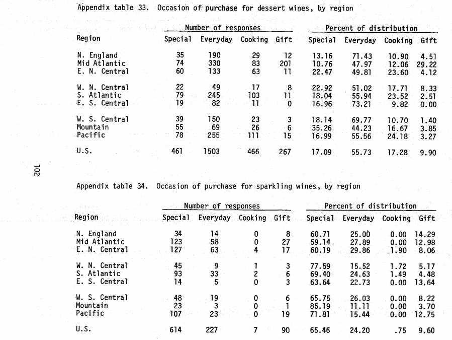
7\ppéndix table 33. Occasion oft purchase for dessert wioes, by^^^

Region

N. England Mid Atlantic E.N. Central

W/ N. Central S. Atlantic E. S. Central

W. S* Central Mountain Pacific

U.S.

Number of responses Percent of distnbutioh Speci al Everyday Cooking Gift Special Everyday Cooking Gift

35 74 60

190 330 133

29 83 63

12 201

11

13.16 10.76 22.47

71.43 47.97 49.81

10.90 12.06 23.60

4.51 29.22 4.12

22 79 19

49 245

82

17 103

11

8 11

0

22.92 18.04 16.96

51.02 55.94 73.21

17.71 23.52 9.82

8.33 2.51 0.00

39 55 78

150 69

255

23 26

lit

3 6

15

18.14 35.26 16.99

69.77 44.23 55.56

10.70 16.67 24.18

1.40 3.85 3.27

461 1503 406 267 17.09 55.73 17.28 9.90

o rs3

Appendix table 34. Occasion of purchase for sparkling wines, by region

Number of responses Percent of distribution Region

N. England Mid Atlantic E. N. Centr'al



Spécial Everyday Gopking Gi-ft SpeGial E\^ery<tey Cooking Gift

34 14 123 58 127 63

45 9 93 33 14 5

48 19 23 3

107 23

0 0 4

1 2 0

0 0 0

8 27 17

3 6 3

6 1

19

60.71 59.14 60,19

77.59 69.40 63.64

65.75 85.19 71.81

25.0Ö 27.89 29,86

15.52 24.63 22.73

26.03 11,11 15.44

0.00 14.29 0.00 12.98 1.90 8.06

1.72 1.49 0.00

5.17 4.48

13.64

0.00 8.22 0,00 3.70 0.00 12.75

U.S. 614 227 90 65.46 24.20 .75 9.60

Appendix table 35. Occasion of purchase for flavored wines, by region

Number responses Percent of distribution

Region

N. England Mid Atlantic E. N, Central




40 65 120 179 188 379

43 107 88 195 23 33

51 TOO 37 66

131 272

1 1

10

17 9 7

3 5 8

5 23 30

16 6 5

7 1 5

36.04 37.15 30.97

23.50 29.53 33.82

31.68 33.95 31.49

58.56 55.42 62.44

58.47 65.44 48.53

62.11 60.55 65.39

.90 4.51

.30 7.12 1.65 4.94

9.29 3.02

10.29

1.86 4.59 1.92

8.74 2.01 7.35

4.35 .92

1.20

U.S. 721 1396 61 98 31.68 61.34 2.68 4.31

o

Appendix table 36. Occasion of purchase for vermouth wines, by region


Region





3 14 11 79 10 67

2 0 10 36 3 19

0 2 0 21

12 42

3 13

5

0 4 8

2 4 6

0 0 0

0 0 0

0 0 1

15.00 10.68 12.20

100.00 20.00 10.00

0.00 0.00

19.67

70.00 76.70 81.71

0.00 72.00 63.33

50.00 84.00 68.85

15.00 0.00 12.62 0.00 6.10 0.00

0.00 8.00

26.67

50.00 16.00 9.84

0.00 0.00 0.00

0.00 0.00 1.64

U.S. 51 280 45 13.53 74.27 11.94 .27

Appendix table 37. Occasion of purchase for brandy wines, by region


o 4S*

Region




U.S.


1 0 9 5 8 6

0 6 2 10 0 1

0 1 0 0 8 17

28 46

0 0 2

1 3 2

0 0 4

12

1 2 1

0 0 0

0 0 2

50.00 56.25 47.06

0.00 13.33 0.00

0.00 0.00

25.81

30.44

0.00 31.25 35.29

85.71 66.67 33.33

100.00 0.00

54.84

0.00 50.00 0.00 12.50

11.77 5.88

14.29 0.00 20.00 0.00 66.67 0.00

0.00 0.00

12.90

0.00 0.00 6.45

50.00 13.04 6.52

Appendix table 38. Persons who drink varietal wine, by region


Region Panel member


Panel member



85 385 332

59 351 309

7 52 30

57 278 216

49 196 201

33.07 30.51 30v52

22.96 27.81 28.40

2.72 4.12 2.76

22.18 22.03 19.85

19.07 15.53 18.47


136 194

26

136 185

26

18 18

4

92 158

19

90 90 13

28.-81 30.08 29.55

28.81 28.68 29.55

3.81 2.79 4.55

19.49 24.50 21.59

19.07 13.95 14.77


87 69

585

88 65

562

6 7

40

51 37

371

38 23

371

32.22 34.33 30.33

32.59 32.34 29.13

2.22 3.48 2.07

18.89 18.41 19.23

14.07 11.44 19.23

U.S. 1899 1781 182 1279 974 31.06 29.13 2.98 20.92 15.93

o

Appendix table 39. Persons who drink nonyarietal wines, by region


Region Panel member


Panel member



615 1561 1307

501 1451 1199

42 136

94

386 1194

765

331 824 572

32.80 30.22 33.20

26.72 28.09 30.46

2.24 2.63 2.39

20.59 23.11 19.43

Í7.65 15.95 14.53


381 866 159

332 815 159

20 63 12

255 622 100

208 431

79

31.86 30.96 31.24

27.76 29.14 31.24

1.67 2.25 2.36

21.32 22.24 19.65

17.39 15.41 15.52


469 313

2840

449 298

2686

26 18

167

307 202

1939

212 120

1390

32.06 32.91 31.48

30.69 31.34 29.77

1.78 1.89 1.85

20.98 21.24 21.49

14.49 12.62 15.41

U.S. 8511 7890 578 5725 4167 31.67 29.36 2.15 21.31 15.51

Appendix table 40, Persons who drink dessert wines, by region

Region

N. England Hid Atlantic E. N. Central

Number of responses

Panel Male member head

190 151 362 303 209 156

Children Friends Relatives

9 117 19 247 5 100

85 243 86


Panel Male member head Children Friends Relatives

34.42 27.36 30.84 25.81 37.59 28.06

1.63 1.62

.90

21.20 21.04 17.99

15.40 20.70 15.47

W. N. Central 75 48 1 44 32 S. Atlantic 270 227 8 194 131 E. S. Central 45 80 2 37 23

37.50 24.00 32.53 27.35 24.06 42.78

.50

.96 1.07

22.00 23.37 19.79

16.00 15.78 12.30

W. S. Central 130 148 11 103 80 Mountain 109 107 2 70 42 Pacific 334 267 20 168 119

27.54 33.03 36.78

31.36 32.42 29.41

2.33 .61

2.20

21.82 21.21 18.50

16.95 12.73 13.11

U.S. 1724 1487 77 1080 841 33.10 28.55 1.48 20.73 16.15

o cri

Appendix table 41. Persons who drink sparkling wines, by region

Nurfiber of responses Percent of distribution

Panel Male Panel Male Region member head Children Friends Relatives member head Children Friends Relatives

N- England 47 37 2 30 21 34, .31 27, .01 1, .46 21, .90 15, .33 Mid Atlantic 167 136 19 102 90 32. .49 26, .46 3, .70 19.84 17. .51 E. N. Central 165 146 18 92 87 32.48 28, .74 3, .54 18. .11 17. .13

W. N. Central 46 40 8 19 32 31, ,72 27, .59 5, .52 13. ,10 22. .07 S. Atlantic 108 105 8 75 42 31, .95 31, .07 2, .37 22. ,19 12. ,43 E. S. Central 13 15 4 9 6 27, .66 31, ,92 8, .51 19. ,15 12. ,77

W. S. Central 52 49 7 39 30 29, ,38 27. ,68 3. .96 22. ,05 16. .95 Mountain 24 23 1 18 13 30; ,38 29. ,11 1. .27 22. .79 16. ,46 Pacific 131 112 28 39 55 35. ,89 30. ,69 7. .67 10. 69 15. ,07

U.S. 753 663 90 473 376 31.98 28.15 3.82 20.09 15.97

Appendix table 42. Persons who drink flavored wines, by region


Region Panel member


Panel member



91 264 461

68 227 416

0 56 59

67 172 271

51 162 220

32.85 29.97 32.31

24.55 25.77 29.15

0.00 6.36 4.14

24.19 19.52 18.99

18.41 18.39 15.42


151 236 42

118 198

36

18 21

7

109 167 35

76 82 27

31.99 33.52 28.57

25.00 28.13 24.49

3.81 2.98 4.76

23.09 23.72 23.81

16.10 11.65 18.37


132 96

345

112 80

269

14 14 39

87 65

191

51 33

143

33.33 33.33 34.95

28.28 27.78 27.25

3.54 4.86 3.95

21.97 22.57 19.35

12.88 11.46 14.49

U.S. 1818 1524 228 1164 845 32.59 27.34 4.09 20.86 15.15

o

Appendix table 43. Persons who drink vermouth wines, by region

Region




Panel Male member head

17 66 63

0 27 23

3 19 47

Number of responses

15 73 59

1 19 22

2 21 47

Children Friends Relatives

0 4 3

0 0 0

0 0 0

14 52 51

2 22 12

0 18 35

12 52 29

0 20 1

0 13 18

Percent of distribution Panel Male member head Children Friends Relatives

29.31 25.86 26.72 29.56 30.73 28.78

0.00 33.33 30.68 21.59 39.66 37.93

60.00 26.76 31.97

40.00 29.58 31.97

0.00 1.62 1.46

0.00 0.00 0.00

0.00 0.00 0.00

24.14 21.05 24.88

66.67 25.00 20.69

0.00 25.35 23.81

20.69 21.05 14.15

0.00 22.73 1.72

0.00 18.31 12.25

U.S. 265 259 206 145 30.05 29.37 .79 23.36 16.44

Appendix table 44. Persons who drink brandy wines, by region


Region Panel member


Panel member



2 10 14

1 9

15

0 1 2

2 11 12

2 11 12

28.57 23.81 25.46

14.29 21.43 27.27

0.00 2.38 3.64

28.57 26.19 21.82

28.57 26.19 21.82


7 13

3

5 11

0

0 0 0

6 11

1

3 6 0

33.33 31.71 75.00

23.81 26.83 0.00

0.00 0.00 0.00

28.57 26.83 25.00

14.29 14.63 0.00


1 0

27

1 0

20

0 0 0

0 0

19

0 0

14

50.00 0.00

33.75

50.00 0.00

25.00

0.00 0.00 0.00

0.00 0.00

23.75

0.00 0.00

17.50

U.S. 77 62 62 48 30.56 24.60 1.19 24.60 19.05

o CO

Appendix table 45. Place of purchase for varietal wines, by region


Region Supermarket Liquor store

Drug store Other Supermarket

Liquor store

Drug store Other


23 16

228

67 387 138

4 1

26

6 2

21

23.00 3.94

55.21

67.00 95.32 33.41

4.00 .25

6.30

6.00 .49

5,09


43 136

7

110 84 25

4 7 1

7 10

1

26.22 57.38 20.59

67.07 35.44 73.53

2.44 2.95 2.94

4.27 4.22 2.94


50 26

386

45 41

125

5 2

33

7 4

94

46.73 35.62 60.50

42.06 56.16 19.59

4.67 2.74 5.17

6.54 5.48

14.73

U.S. 915 1022 83 152 42.13 47.05 3.82 7.00

Appendix table 46, Place of purchase for nonvarietal wines, by region



Liquor store

Drug store Other


202 123 945

479 1589 422

2 2

69

29 72 93

28.37 6.89

61.81

62.28 88.97 27.60

.28

.11 4.51

4.07 4.03 6.08


76 738

42

344 264 140

9 33

6

26 42

5

16.70 68.52 21.76

75.60 24.51 72.54

1.98 3.06 3.11

5.71 3.90 2.59

W. S. Central Mountain Paci fi c

339 189

2313

177 133 495

20 16

151

27 24

219

60.21 52.21 72.78

31.44 36.74 15.58

3.55 4.42 4.75

4.80 6.63 6.89

U.S. 4967 4043 308 537 50.40 41.03 3.13 5.45

o

Appendix table 47. Place of purchase for dessert wines, by region




Liquor store

Drug store Other


25 33

155

199 372

59

2 10 16

12 17 11

10.50 7.64

64.32

83.63 86.11 24.48

.84 2.32 6.64

5.04 3.94 4.56

W. N. Central S. Atlantic S. E, Central

29 227

4

50 89 92

8 7 2

2 14

8

32.58 67.36 3.77

56.18 26.41 86.79

8.90 2.07 1.89

2.25 4.15 7.55


125 28

307

67 77 43

5 7

15

3 18 42

62.50 21.54 75.43

33.50 59.23 10.57

2.50 5.39 3.69

1.50 13.85 10.32

U.S. 933 1048 72 127 42.80 48.07 3.30 5.83

Appendix table 48. Place of purchase for sparkl" ing wines, by region

Number of resDonses_ Percent of distribution

Region Supermarket Liquor Drug store store Other Supermarket

Liquor store

Drug store Other

N. England Mid ÄtTantic E. N. Central

11 13 94

40 0 178 0

59 26

5 7

13

19.64 6.57

48.96

71.43 89.90 30.73

0.00 0.00

13.54

8.93 3.54 6.77


20 83

1

25 10 37 4 20 0

0 6 0

36.36 63.85 4.76

45.46 28.46 95.24

18.T8 3.08 0.00

0.00 4.62 0.00


30 IT 87

26 .3 14 2 38 n

7 0

12

45.46 40.74 58.78

39.39 51.85 25.68

4.55 7.41 7.43

10.61 0.00 8.11

U.S. 350 437 56 50 39.19 48.94 6.27 5.60

Appendix table 49. Place of purchase for flavored wines, by region

Number of responses Percent of distribytion



Liquor store

Druig store Other

N. England Mid ÄtTantic E. N. CentraT

41 23

407

59 258 1T8

0 0

25

8 27 24

37.96 7.47

70.91

54.63 83.77 20.56

0.00 0.00 4.36

7.41 8.77 4.18


43 211

18

107 45 23

17 4

15

16 21

3

23.50 75.09 30.51

58.47 16.01 38.98

9.29 1.42

25.42

8.74 7.47 5.09

W. S. Central Mountain Paci fi c

95 49

319

45 39 31

8 10 14

8 5

29

60.90 47.57 81.17

28.85 37.86 7.89

5.13 9.71 3.56

5.13 4.85 7.38

U.S. 1206 725 97 141 55.60 33.43 4.47 6.50

Appendix table 50. Place of purchase for vermouth wines, by region


Region

N. England Mid Atlantic E. N, Central



U.S.

Supermarket

0 10 66

1 24

1

1 10 31

144

Liquor store

18 78 10

1 9

22

1 0

20

159

Drug store

0 0 1

0 2 0

0 8 1

12

Other

0 0 1

0 5 0

1 3 5

15

Supermarket

0.00 11.36 84.62

50.00 60.00 4.35

33.33 47.62 54.39

43.64

Liquor store

100.00 88.64 12.82

50.00 22.50 95.65

33.33 0.00

35.09

48.18

Drug store

0.00 0.00 1.28

0.00 5.00 0.00

0.00 38.10 1.75

3.64

Other

0.00 0.00 1.28

0.00 12.50 0.00

33.33 14.29 8.77

4.55

Appendix table 51. Place of purchase for brandy wines, by region


Region Supermarket Li quor store


Liquor store

Drug store Other


0 0 3

2 14

9

0 0 3

0 1 1

0.00 0.00

18.75

100.00 93.33 56.25

0.00 0.00

18.75

0.00 6.67 6.25


0 1 1

6 12

2

1 0 0

0 0 0

0.00 7.69

33.33

85.71 92.31 66.67

14.29 0.00 0.00

0.00 0.00 0.00

W. S. Central Moutain Pacific

0 0

19

1 0 7

0 0 3

0 0 0

0.00 0.00

65.52

100.00 0.00

24.14

0.00 0.00

10.34

0.00 0.00 0.00

U.S. 24 53 27.91 61.63 8.14 2.33

Appendix table 52. Average prices paid and market share by major wineries for domestic varietal table wine, by region

Wine company

New England

Middle Atlantic

East North Central

West North Central

South East South Atlantic Central

Average price Cents per pound

West South Central Mountain Pacific

TotaT all regions

Gallo United Vintners Franzi a

6.1 3.4

6.2 5.3 4.5

6.0 6.0 4.0

4.9 4.6

6.4 5.3 4.7

6.5 5.4 4.5 4.0

5.0 5.7

6.1 3.8 3.4

6.0 4.5 3.7

' Mögen David Almadén Canadaigua

5.2 7.2

6.1 7.4

6.0 6.9 6.0

6.6 6.4 8.5

7.2 14.6

5.0 7.8

6.6 7.4 7.8

6.0 7.5 6.0

Guild Taylor Paul Masson 11.7

3.9 6.3 7.7

5.6 8.7 8.6

8.3 15.5

9.2 5.0

11.6 11.4

9.3 6.8

4,3

10.0

4.4 8.6 9.6

Christian Brothers California Wine Great Western 6.4

12.1

6.1

13.8 10.3 10.1 4.1

7.0 11.8 3.3

11.5 3.8 6.2

-. Gold Seal S Other wine companies

Total average

6.6 5.6 5.3

5.3 6.8 6.1

5.2 7.0 6.3

5.1 7.7 6.8

6.3 9.3 6.4

12.9 8.8

8.4 5.7

8.2 5.8 6.1

7.3 5.8

5.5 7.2 6.1

Market share Percent


7.7 21.5

7.9 19.2

.6

8.7 12.7 1.4

1.5 30.7

5.5 40.3

2.4

4.8 8.5 11.9 1.8

7.3 9.7

4.2 37.1 5.2

6.1 26.1 2.4

Mögen David Almaden Canadaigua

6.2 4.2

7.8 6.8

33.0 6.6 5.1

20.6 21.9 1.6

63.6 4.8

55,7 1.4

28.3 .8 2.7

15.9 3.8 .8

Guild Taylor Paul Masson .9

2.9 .5 .5

1.9 .5 .5

1.8 3.6

1.3 1.8

4.8 9.6

.7 11.3

1.4

1.5

1.3 .5

1.5


.5

2.2

.5 .8 .9 2.2

.7 1.7 .3

.9

.3

.5

GQld Seal Other wine companies Total

3.8 54.0

100.0

13.4 37.7

100.0

6.1 22.9

100.0

1.5 39.5

100.0

5.0 17.1

100.0 12.4

100.0 19.2

100.0

1.6 41.8

100.0 45.0

100.0

4.4 35.3

100.0

Appendix table 53. Average prices paid and market share by major wineries for domestic nonvarietal table wine, by region

Wine company


Mögen David Almadén Canadaigua

Guild Taylor Paul Masson

Christian Brothers California Wine Great Western

z: Gold Seal ^ Other wine companies

Total average

New England

Middle Atlantic

East North Central

West North Central

South Atlantic

Average Cents pel

East South Central

price r pound

West South Central

4.8 4.6 4.9

4.3 4.8 4.2

4.6 4.9 4.1

4.1 4.0 3.0

4.7 6.0 4.7

4.7 6.4 4.1

4.0 4.0 4.6

6.4 5.9 3.9

5.7 6.3 7.6

4.2 6.3 5.9

6.4 6.3

5.4 6.0 5.3 6.1

4.7 5.1 4.7

3.7 5.7 7.3

4.3 7.5 8.2

4.1 8.3 7.8

4.0 6.7 7.9

3.5 7.S 7.9

5.0 8.0 7.8

4.3 7.2 4.1

Mountain Pacific Total all regions

7.0

7.8

5.5 4.1 4.7

8.3 2.3 5.4

5.0 5.5 5.2


30.1 9.7

.1

31.8 10.8

.4

44.0 15.3

.7


.1 8.5 1.9

.2 7.1

.6

.3 3.8 1.5


4.5 4.7 2.7

1.1 2.8 1.4

6.1 2.3 2.1


1.2 2.5

.3

.5

1.7

4.1 .6 .4

Gold Seal .3 1.0 .2 Other wine companies Total

33.4 100.0

40.6 100.0

18.6 100.0

8.3

4.9 5.5 4.9

42.3 14.5 1.1

.9

.2

1.1 4.2 3.8

3.1

.9 28.0

100.0

3.0

8.0

8.9 15.6

3.9 4.0 4.8

6 5

.2

.5


29.0 10.0 7.9

47. 7. 3.

.8

.5 ,5

.1 6.1 2.2 5

7.9 5.5 1.5

16. 8. 4.

8 3 0

1.2

.1

.1 28.5

100.0 10.8

100.0

9.4 2.4 7.8

4.0 4.5

3.4 4.2 3.0

3.6 4.4 3.1

4.1 4.6 3.8

4.5 5.0 5.1 5.6 5.5

4.7 6.2 7.8

3.2

6.7

3.6 7.3 7.3

3.8 2.5

3.4 4.0

10.7

6.6 2.9 7.5

3.7 3.9

2.9 3.5

5.4 3.7 4.3

39,0 9.2 2.0

29.1 20.1 1.6

28.5 11.5 2.9

32.7 11.9 2.3

.1 11.6 1.4

3.4 4.4 .1

5.5 .7

.1 3.6 1.7

2.2 2.1 4.0

6.6

1.8

4.7 2.3 2.0

3,8 1.0

.1

1.6 10.2

1.0 .2

1.6 .8 .4

26.3 100.0

25.7 100.0

43.0 100.0

.3 34.8

100.0

Appendix table 54. Average prices paid and market share by major wineries for domestic dessert wine, by region

Wine company

New England

Middle Atlantic

East North Central

West North Central

South Atlantic

East South Central


Total all regions



3.0 3.9

4.6 5.2

4.8 4.1 6.1

5.2 3.4 5.0

5.7 4.8 5.5

6.5 5.5

4.0 5.0 3.9

3.6 3.9

4.0 5.0 4.0

4.5 4.6 5.0

Mögen David Almadén Canädaigua

5.7 7.0 7.7 5.3 8.0 9.5 5.2 7.3 7.1

5.3 6.9

Guild Tayler Paul Masson

3.9 6.0 7.9

4.7 8.0 8.7

4.6 8.1 7.7

7.0 10.1

4.7 8.0 6.8

5.3 8.9 6.1

6.9 4.9 6.5 5.5

7.0

16.9

4.8 7.2 9.T

Christian Brothers California Wiwe Rreait Western

7.0 3.6 6.7

7.3

9.8

8.8 8.2 12.3 7.6 7.9

7.8

6.1 8.1 8.2 3.6 9.5

=:: Gold Seat ■^ Other wine companies

Total Average 5.4 5.0

4.9 5.7

5.8 5.7

5.7 6.2

11.4 6.2

6.3 6.6

3.4 5.7

5.2 4.3

4.9 5.3

5.2 5.6


Gallo United Vintners Franzia

13.4 9.9

45.7 3.7

39.4 13.9

.5

24.3 6.2 2.7

32.8 28.7 2.8

41.2 4.3

18.8 1,7

.6

63.9 4.3

55.1 5.5

.9

39.4 8.7

.7

Mögen David Almaden Canädaigua

7,8 3.1 5.5 1.7

14.4 1.2 4.7 1.2 7.0 .1

4.4


10.2 19.5 4.1

.2 8.8 2.2

2.6 10.2 4.5

18,5 2.7

6.3 20.7 2.8

17.0 17.0 2.4

57.2 ,6

11,0 1.5

2.0

9.8

3.5 15.2 3.8


.4

.5 1.9

4.0

9.0

6.1 2.7 2.4 4.3 2.8

.6

1.5 4.4 3.3 .1

2.6

Gold Seal Other wine companies Total

32.3 100.0

23.2 1Ö0.0

17.3 100.0

26.6 100.0

2.4 100.0

9.2 100.0

18.4 100.0

15.9 100.0

15.3 100.0

18.4 100.0

Appendix table 55. Average prices paid and market share by major wineries for domestic sparkling wine, by region

Wine company



Guild Tayl or Paul Masson


- Gold Seal îj; other wine companies

Total average

Gallo United Vintners Franzla




GoTd Seal Other wine companies Total

New England

Middle Atlantic

East North Central

West North Central

South Atlantic

East South Central

West South Central Mountain


13.8 11.7 7.4

9.2 10.9

7.5 8.6 7.3

8.3

7.7

8.3 8.2 9,8

10.2 9.6 9.1

6.8

7.8 11.7 7.3

4.3 13.7

3.9 19.5

6.5 4.0 5.6 13.6

17.4 8.1

10.1 8.7

19.7 14.3

18.2 15.1 14.0

4.7 21.9

36.7 17.9 9.2

7.2

Pacific Total all

regions

11.5

9.6 12.7

41.3 1.8

10.1

3.7 3.7

12,8

17.4

9.2 100.0

17.3

7.0 10.9 9.9

40.8 .7

8.9 14.6

4,0

4.8 25.3

100.0

12.7

14.8 9.1 8.3

62.3 7.0 3.7

1.2

4.9 1.6 2.9

.8

.4 15.1

100.0

19.8

9.6 9.1

56.8

1.5

1.9

4.6

9.4

19.1 10.1 9.3

5,6 9.7

Market share Pêircént

66,4 2.8 4.4

.9

.9

7.8 .9

1.7

23. 23,

19.2 7.7

7.7

7.9 9.0

49.9 4.6 4.3

1.7 7.0

.9

7.8

7.5 7.8 7.8

8.3 8.4

12.2

15.7 5.1

15.5

7.6

12.7

9.2 13.4 13.5

19.8

14.0

8.9 8.3

8.4 9.5 9.2

62.7 3.4

27.1

46.2 20.8 1.7

51.6 6.5 3.4

3.4 .8 .9

6.8 3.4

1.3

4.5 6.6 1.0

2.2

.9 35.1 13.3 19.2

100.0 100.0 100.0 31.6

100.0 100.0

1.4 23.3 21.1

100.0 100.0

Appendix table 56. Average prices paid and market share by major wineries for domestic flavored wine, by region

Wine company

New England

Middle Atlantic

East North Central

West North Central

South Atlantic

East South Central


Total all regions



3.9 3.6

4.5 5.2

5.0 4.9

4.3 5.1

5.2 6.6

5.5 4.7

4.5 3.7 9.6

3.2 4.7

4.0 4.6

4.5 4.9 9.6


6.5

4.5

6.6

3.9

6.0 7.8 4.5

5.1

7.6

6.3

5.3

7.4 6.4 5.9

5.5 6.0 3.3

5.9 5.0 5.1


5.0 8.9

7.0 9.0 8.6

6.0 8.4 7.9

8.6 8.2

5.9 7.2 7.3

7.4 1.6 5.8 7.5

5.4 7.8 6.2

6.4

7.7

4.4 7.8 7.6


9.4 7.4 11.7

8.4 11.7

_^ Gold Seal ^ Other wine companies ^ Total average

5.5 4.4

6.6 5.5

5.7 5.3

6.6 5.1

6.9 6.0

9.1 6.1

5.1 4.8

4.7 4.2

6.8 4.6

6.2 5.2


Gal To United Vintners Franzi a

50.8 15.3

50.4 14.8

46.6 10.6

41.9 17.0

44.2 10.5

61.7 8.9

38.4 7.6

. 2.5

47.2 23.9

68.0 14.5

50.4 13.6

.1


7.1

2.7

2.4

.3

19.4 .2

1.9

18.1

1.0

12.4

1.9

4.3 1.7 6.0

18.8 4.3 .7

10.0 .2

1.1


5.6 .9

.3 5.5

.6

.2 ,4 .6

.5 1.4

1.8 2.9 1.4

3.4 4.1

.8 1.1

.7 4.0 2.3

.3

1.1

.6 2.1 1.0


.4 .8 .3

.1

.1


17.6 100.0

25.7 100.0

20.0 100.0

20.0 100.0

24.6 100.0

14.0 100.0

25.9 100.0

17.6 100.0

15.2 100.0

20.5 100.0

Appendix table 57. Average prices paid and market share by major wineries for vermouth, by region

Wine company


Mögen David Alamden Canadaigua



- Gold Seal ^ Other wine companies

Total average

New England

Middle Atlantic

East North Central

West North Central

South Atlantic

East South Central


Total all regions


3.7 6.9 5.7

6.0 7.5 4.0

5.8 5.9 5.8

5.7 5.0 7.5

4.6

3.9

4.9 4.9 4.3

5.7 5.5 5,0

10.5 5.3 6.0 8.9 8.0

7.6 7.0 6.0 8.0

5.8 7.1 6.0

10.1 6.6

8.1 6.6

6.4

4.3

6.2

8.1 6.6 6.2

5.1

7.2 5.4

7.2 5.4 5.1

5.4 5.4

5.6 5.7

8.0 7.1 6.7

5.2 6.0

7.7 6.5 6.4 4.3

5.4 5.3

6.1 6.0


24.5 2.3

14.4 39.8 2.5


6.5 18.2 9.3

Guild Tayl or Paul Masson

16.3 5.9 2.6

5.0 2.5


3.1


46.1 100.0

56.6 100.0

37.9 100.0


33.3

66.7

100.0

19.7 17.6 14.1

2.8 2.8

22.5

5.6

14.8 100.0

30.8

7.7

46.2

44.4 55.6

15.4 100.0 100.0

50.0

50.0

24.8 10.6 10.6

15.4 14.4 4.4

3.5 10.2 .4

3.5

24.8

2.4 7.3 6.7

.5

.9

.4

00.0 22.1

100.0 36.9

100.0

Appendix table 58. Average prices paid and market share by major wineries for domestic brandy, by region

Wine company

New England

Middle Atlantic

East North Central


32.1 33.2

Moäen David Almadén Canâdaigua



19.6

Gold Seal ptheY' wirie companies Total average

14.6 16.2

19.2 20.3

14.9 16.8

Galio United Vintners Franzia

7.2 10.1

Mögen David Almadén Canâdaigua



40.1


60.0 100.0

52.7 100.0

89.9 100.0

West North Central

16.1

13.7

5.0 13.8

50.0

37.5

12.5 100.0

South Atlantic

East South Central


6.6 18.0

19.5

12.7

14.1 16.0

2.7 2.7


16.4 7.7

53.8

7.7

15-4 lOO.Q

100.0 100.0


14.0

14.0

100.0

19.5

5.5

12.6 11.8

15.0

100.0

26.2

58.9 100.0

Total all regions

6.6 19.2

13.7 19.5

18.7

12.6

13.4 14.9

3.3 18.0

6,2 11.6

1.0

13-3

46.5 100.0

Appendix table 59. Average prices paid and market share by major wineries for domestic other wine, by region

Wine company

New Middle East North West North South East South West South Total all England Atlantic Central Central Atlantic Central Central Mountain Pacific regions



3.2 6.2 4.9



5.5 6.6

5.3

5.5 6.6

5.3


Gold Seal Other wine companies Total average

7.6 6.7

7.8 7.8

20. 20,

7.9 7.9

9.0 7.1

7.8 7.8

7.3 7.3

5.4 5.6

3.9 3.9

Market s-hare Percent

8.8 8.1


16.4 26.9 7.1


42.1 15.4

7.9 3.0


16.4 3.2



57.9 100.0

100.0 100.0

100.0 100.0

100.0 100.0

51.7 100.0

100.0 100.0

100.0 100.0

73.1 100.0

100.0 100.0

78.9 100.0

Appendix table" 60. Household demographics and wine purchasing patterns for those purchasing less wine, New England region

Wine type purchased


Age of Education wife of male Years head a/

, _ ^ _ _ nAITIûC ^ í r>



1 3 3

25 5.0 32 3.5 35 5.0

9,500 9,167

10,167

Sparkling Flavored

1 1

65 3.0 35 4.0

9.500 17,500

iinporuea —--

Nonvarietal table Fîavored Vermouth

1 1 1

35 4.0 45 2.0 35 5.0

17,500 10,500 10.500

Other 25 4.0 10,500

a/ Education codes: 1 - grade school; 2 - some high school; 3 - graduated high school; 4 - some college; 5 - graduated college or more.

Appendix table 61. Household demographics and wine purchasing patterns for those purchasing more wine. New England region

Wirve type purchased


Age of wife Years



Domestic


Sparkling Flavored Other

Nonvarietal table Dessert

1 14

6

2 3 1

25 38 38

40 35 35

4.0 3.5 3.7

2,0 2.3 4.0

Imported

38 42

3.3 3.3

14,000 14,643 15,250

11.000 12,000 12,500

14,167 12,000


120

Appendix table 62. Household demographics and wine purchasing patterns for those purchasing the same wine. New England

Wine type purchased

Age of Education Household Number of wife of male income households Years head a/ Dollars

Domestic

Varietal table Nonvarietâl table Dessert

Sparkling Flavored Brandy

Other

3 35 8

8 6 1

28 32 39

30 28 15

25

4.0 4.0 5.0

5.0

13,333 16.729 15,125

13,938 14.333 17,500

14,000

Nonvarietâl Dessert Sparkling

table 14 2 1

iiiipt

29 40 45

jrteu

4.1 4.5 3.0

17,679 20,000 17,500

Flavored Vermouth

3 1

35 35

3.0 4.0

13,000 22,500


Appendix table 63. Household demographics and wine purchasing patterns for those purchasing less wine. Middle Atlantic region

Wine type purchased



Household income

Dollars

Varietal table Nonvarietâl table Dessert

4 16

7

38 4.8 34 3.7 36 3.4

12,750 14,344 13,857


2 4 1

25 4.5 40 3.8 25 5.0

17,500 15,000 17,500

Nonvarietâl table Flavored Other

9 1 1

36 3.9 15 3.0 25 2.0

15,222 17,500 17,500


121

Appendix table 64. Household demographics and wine purchasing patterns for those purchasing more wine. Middle Atlantic region

Wine type purchased


Age of wife

Years



_, r\r\ma e>-h 4 r* .


13 55 13

uyjui

31 33 41

CO o I u

4.2 4.0 3.6

16,346 16,891 15,808


11 19

5

32 33 27

3.7 3.7 4.5

17.091 14,184 13,000

Brandy Other

2 2

40 40

Tirir\

5.0 4.0

18,250 20,000

XHipVI UCU

Nonvarietal Dessert Sparkling

table 35 5 1

30 33 25

4.3 4.6 5.0

16,657 19,800 22,500

Flavored Vermouth

8 4

30 23

3.5 4.3

15,188 18,750

a/ Education codes: 1 - grade school; 2 - some high school; 3 - graduated high school; 4 - some college; 5 - graduated college or more r

122

Appendix table 65. Household demographics and wine purchasing patterns for those purchasing the same wine. Middle Atlantic region

Mine type purchased


Age of wife Years



Domestic



Brandy

38 87 17

26 29

3

37 34 41

33 34 45

45

4.0 3.9 4.1

4.3 3.5 4.3

2.7

16,711 15,161 15,176

17,038 13,569 18,833

11,500


2 39

3

—-— imp!

35 33 32

jriea

4.0 4.2 5.0

17,000 16,449 22,500


1 13

3

25 30 38

5.0 4.1 4.7

17.500 14,192 20,833

Brandy Other

2 1

35 35

5.0 5.0

15,000 22,500


123

Appendix table 66. Household demographics and wine purchasing patterns for" ttiose purchasing less wine. East North Central region

Wine type purchased


Age of wife Years



Domestic



Other

7 13

9

3 12

2

1

34 40 45

32 30 50

55

3.3 3.3 2.6

3.3 2.9 3.0

1.0

15,071 13,538 15,167

14,667 10,667 12,000

4,000

Nonvarietal table Dessert Sparkling

3 1 2

Imported

32 65 45

3.7 4.0 3.5

7,333 4.000

20,000


124

Appendix table 67. Household demographics and wine purchasing patterns for those purchasing more wine, East North Central region

Wine type purchased


Age of wife Years



Domestic



Brandy

18 63

7

13 23

2

1

34 35 35

33 34 50

25

4.0 4.0 4.4

3.8 3.6 2.5

3.0

17,111 17,278 19,143

16,923 15,674 11,750

11,500

Imported

Nonvarietal table Dessert Flavored

Vermouth Brandy

29 1 6

1 1

29 35 40

25 25

4.0 2.0 4.2

5.0 3.0

16,155 17,500 17,167

22,500 14,000

a/ Education codes: 1 - 3 - graduated high school college or more.

grade school; 2 - some high school; 4 - some college; 5 - graduated

125

Appendix table 68. Household demographics and wine purchasing patterns for those purchasing the same wine. East f^orth Central region

Wine type purchased


Age of wife Years



n/^mac-i-i/«


32 82 15

38 38 40

3.5 4.0 3.9

15.813 16,683 15,400


21 48

5

38 34 45

4.0 3.6 4.3

18,262 15,625 12,800

Brandy Other

3 1

45 15

, _ Tmn

4.3 5.0

17,500 8,500

xiiipuf ucu


38 3

13

35 28 33

4.0 4.7 3.5

17,816 19,167 16,846

Vermouth Other

2 1

45 25

5.0 5.0

15.000 17,500

a/ Education codes: 1 - 3 - graduated high school college or more.

grade school; 2 - some high school; 4 - some college; 5 - graduated

Appendix table 69. Household demographics and wine purchasing patterns for those purchasing less wine. West North Central region

Wine type purchased


Age of wife Years



Domestic

Varietal table 1 55 2.0 4,000 Nonvarletal table 6 37 3.5 15,417 Dessert 1 25 3.0 8,500

Flavored 3 58 2.3 9,333

Nonvarletal table

— Imported —

25 3.0 17,500

a/ Education codes: 1 - grade school; 2 - some high school; 3 - graduated high school; 4 - some college; 5 - graduated college or more .

126

Appendix table 70. Household demographics and wine purchasing patterns for those purchasing more wine. West North Central region

Wine type purchased



- —-- rinmoc + ir



2 12

5

50 2.5 38 3.7 47 3.0

9.500 16,083 16,500

Sparkling Flavored

2 10

40 4.0 42 3.2

14,250 15,300

importea

Nonvarietal Sparkling Flavored

8 1 2

33 4.0 25 5.0 50 4.5

13,125 22,500 22,500


Appendix table 71. Household demographics and wine purchasing patterns for those purchasing the same wine. West North Central region

Wine type purchased


Age of wife Years



Domestic


Sparkling Flavored

16 35

7

9 22

44 39 39

29 35

3.7 3.8 4.4

3.6 3.8

15,813 15,586 17,429

13,389 14,386

Nonvarietal table Flavored

15 2

Imported

37 35

4.3 5.0

15,667 20,000

a/ Education codes: 1 - grade school; 2 - some high school; 3 - graduated high school; 4 - some college; 5 - graduated college or more*

127

Appendix table 72. Household derrographics and wine purchasing patterns for those {>urctesing less wine, South Atlantic region

Wine type purchased


Age of wife

Years


Household incoine Dollars

Domestic


Sparkling Flavored

3 11

4

2 5

55 39 60

25 49

3.5 4J 4.5

5.0 3.0

6,167 13,864 9,625

12,750 15,500

Nonvarietal table Flavored Brandy

Imported

25 40 55

4,0 4.5 5,0

13,000 9.500

10,500


Appendix table 73. Household demographics and wine purchasing patterns for those purchasing more wine, South Atlantic region

Wine type purchased



———- nnmoc+'ni» _

Household Income Dollars


6 13

4

32 4.6 35 4.7 33 4.3

16,083 18,077 20,375


3 8 2

28 4.7 26 3.9 45 4.5

17,833 14,500 22,500

--^— Imported -■


7 2

34 4.3 45 4.0

19,143 22,500


128

AppeTidix table 74. Household demographics and wine purehasing patterns for those purchasing the same wine. South Atlantic region

Wine type purchased


Age of wife Years



Domestic

Varietal table Monvarietal table Dessert


Other

7 39 U

9 19

3

42 39 46

37 42 38

35

3.7 4.0 3.9

4.7 3.6 4.7

5.0

11,429 15,462 17,714

18,944 16,026 20,833

17.500

Imported

Nonvarietal table Dessert Sparkling

Flavored Vermouth

15 1 1

3 1

33 35 35

25 35

4.1 5.0 5.0

2.5 0.0

17,567 22,500 17,500

12,500 10,500

à/ Education codes; 1 - grade school; 2 - some high school; 3 - graduated high school; 4 - some college; 5 - graduated college or more.

Appendix table 75. Household demographics and wine purchasing patterns for those purchasing less wine. East South Central region

Wine type purchased


Age of wife Years

Education of male

head a/

Household Income

Dollars

Domestic

Non varietal table 1 25 4.0 11,500 Flavored 2 30 4.5 14,500 Vermouth 1 45 3.0 14,000

Non varietal table

— Imported ~

45 3.0 14,000

a/ Education codes: 1 - grade school; 2 - some high school; 3^ graduated high school; 4 - some college; 5 - graduated college or more.

129

Appendix table 76. Household demographics and wine purchasing patterns for those purchasing more w1ne. East South Central region

Wine type purchased


Age of wife Years



Domestic


Fl avored Other

28 35 35

30 15

4.0 4.0 3.0

3.5 5.0

9,833 13,900 12,750

15,750 7,500

Nonvarietal table

— Imported --

35 5.0 22,500

a/ Education codes: 1 - grade school; 2 - some high school; 3 - graduated high school; 4 - son« college; 5 - graduated college or more.

Appendix table 77. Household demographics and wine purchasing patterns for those purchasing the same wine. East South Central region

Wine type purchased

Age of Education Household Number of wife of male Income households Years head a/ Dollars

Domestic



25 35 45

48 49 35

2.7 4.3 4.3

5.0 4.3 5.0

11,333 14,714 19,167

8,333 13,000 17,500

Nonvarietal table

-r^ Imported --

40 3.0 14,250


130

Appendix table 78. Household demographics and wine purchasing patterns for those purchasing less wine. West South Centrar region

Wine type purchased



____ rirnTioc■f"T r^ _____



3 5 2

32 4.0 45 4.4 50 3.0

16,000 15,800 11,750

Sparkling Flavored

1 5

25 3.0 37 3.6

____ Tirrtnnv*^oH __ __

22,500 17,400


4 1

40 3.5 35 3.0

15,375 22,500


Appendix table 79. Household demographics and wine purchasing patterns for those purchasing more wine. West South Central region

Wine type purchased




<>•__■• nomoc^Tí* _____


5 16

2

29 4.4 34 4,2 50 4.0

13,900 15,656 18,250

Sparkling Flavored

4 7

35 4.3 38 3.8

.•___ Tmnnp^ûH __

15,375 16,286


6 2

32 4.5 35 4.0

17,000 12,500


131

Appendix table 80. Household demographics and wine purchasing patterns for those purchasing the same wine. West South Central region

Wine type purchased



Household ineome Dollars


9 23 14

35 4.6 33 4.4 38 3.7

19,889 17,152 14,821


7 7 1

39 4.6 38 3.7 25 4.0

19.000 15,714 8,500


12 3

32 4.3 35 4.7

18,083 16,333

dj Education codes: 1 - grade schoal ; 2 - some high school; 3 - graduated high school; 4 - some college; 5 - graduated college or more.

Appendix table 81. Household demographics and wine purchasing patterns for those purchasing less wine. Mountain region

Wine type purchased


Age of wife Years



Domestic

Varietal table 5 39 4.5 Nonvarietal table 7 42 3.9 Flavored 7 32 3^3

15,100 11,500 11,929

Imported

Nonvarietal table 1 25 Fl avored 1 35

3.0 3.0

11,500 17,500


132

Appendix table 82. Household demographics and wine purchasing patterns for those purchasing more wine, Mountain region

Wine type purchased


Age of wife Years



Domestic


Sparkling Flavored

2 12

1

3 4

30 30 25

32 35

4.0 4.5 3.0

5.0 3.8

18,250 15,375 14,000

20,833 11,625

Nonvarietal table

■- Imported --

37 3.4 15,500


Appendix table 83. Household demographics and wine purchasing patterns for those purchasing the same wine. Mountain region

Wine type purchased





6 19

4

— — — - UUMICO U 1 L. -- —--

48 3.7 39 4.0 50 4.5

14,083 14,316 16,625

Sparkling Flavored Other

5 13

1

41 4.6 38 3.7 20 0.0

15,200 10,846 7,500

---- ilJljJUi LcU —-- —-


8 1

33 4.6 25 0.0

18,563 4,000


133

Appendix table 84. Household demographics and wine purchasing patterns for those purchasing less wine, Pacific region

Wine type purchased

Age of Education Household Number of wife of male income households Years head a/ Dollars

Domestic



Brandy

11 19 8

6 9 1

42 41 48

33 38 25

25

3.6 3.8 3.5

4.0 3.0 5.0

5,0

18,364 17,053 16,875

16,083 11,889 17,500

17,500

Nonvarietal table

~ Imported —

27 3.0 13,300

a/ Education codes; 1 - grade school; 2 - some high schooU 3 - graduated high school; 4 - some college; 5 - graduated college or more.

Appendix table 85. Household demographics and wine purchasing patterns for those purchasing more wine, Pacific region

Wine type purchased

Age of Education Household Number of wife of male Income households Years head a/ Dollars

Domestic



Brandy

22 51 12

7 8 3

34 36 35

35 39 38

25

4.1 4.1 4.4

4.6 3.8 3.7

4.0

19,386 18,069 18,333

18,857 12,188 20,833

20,000


Imported

38 25 35

4.3 4.0 5.0

18,500 18,250 22,500

a/ Education codes: 1 - grade school; 2 - some high school; 3 - graduated high school; 4 - some college; 5 - graduated college or more. ^

134

Appendix table 66. Household demographics and wine purchasing patterns for those purchasing the same wine. Pacific region

Wine type purchased


Age of wife Years^



Hrk mrt Í» +-1 r^


51 137

32

38 39 44

CO o 1 w» - ——

4.2 3.9 3.7

16,098 14,803 14.000


20 39

5

37 38 43

4.3 3.7 3.6

16,075 14,782 16,500

Brandy Other

1 2

45 35

4.0 4.5

jrted

14,000 16.500

"""" impc

Nonvarietal Flavored

table 29 4

42 30

4.4 4.7

18,362 16,750

a/ Education codes: 1 ■ 3 - graduated high school college or more.

grade school; 2 - some high school 4 - some college; 5 - graduated

135

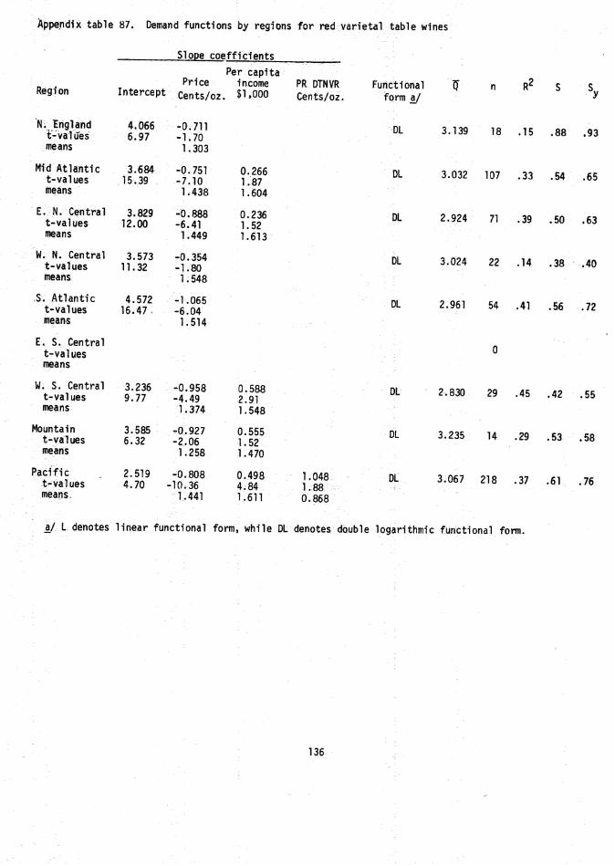
Appendix table 87. Demand functions by regions for red variet&l table wines

Region

Slope coefficients

Per capita Price income PR DTNVR

Cents/02. $1.000 Cents/oz. Intercept Functional Q n R^ S S forma/ ^

Nv England t-vâîûés means

4.066 6/97

-0.711 -1.70 1.303

Mid Atlantic t-va1ues weans

3.684 15.39

-0.751 -7.10 1.438

0.266 1.87 1.604

E.Ñ. Central t-values means

3.829 12.00

-0.888 -6.41

1.449

0.236 1.52 1.613

W. N. Central t-vaTues means

3.573 11.32

-0.354 -Î.80 1.548

S. Atlantic t-values means

4.572 16.47 .

-K065 -6v04

1.514

E. S. Central t-values means

W; S. Central t-values means

3.236 9.77

-0.958 -4.49 1.374

0.588 2.91 1.548

Mountain t-values means

3.585 6.32

-0.927 -2.06

1.258

0.555 1.52 1.^70

Pacific t-values means.

2.519 4.70

-0.808 -10.36

1.441

0.498 4.84 1.611

1.048 1.88 0.868

01- 3.139 18 .15 .88 .93

DL 3.032 107 .33 .54 .65

DL 2.924 71 .39 .50 ,63

DL 3.024 22 .14 .38 .40

DL 2.961 54 ,41 .56 .72

DL 2.330 29 .45 .42 .55

DL 3.235 14 .29 .53 .58

DL 3.067 218 .37 .61 .76

a/ L denotes linear functional form, while DL denotes double logarithmic functional form.

136

Appendix table 88. Demand functions by regions for white varietal table wines

Region

Slope coefficients

Per capita Price income PR DTNVW PR DTVR Functional

Intercept Cents/oz. $1,000 Cents/oz. Cents/oz. forma/

N. England t-values means

3.341 9.70

-0.363 -1.57

1.436

Mid Atlantic t-values means

2.574 7.83

-0.485 -3.60

1.562

0.669 3.99 1.609

E, N. Central t-values means

3.904 16.13

-0.774 -4.66

1.416

W. N. Central t-values means

69.487 2.25

-7.062 -i.n 4.345


3.952 9.11

-0.714 -2.59

1.529


W. S. Central t-values means

21.768 5.00

-3.461 -3,48 4.011

2.606 3.20 4.565


2.081 2.15

-0.682 -3.05

1.393

1.124 1.13 0.905

0,634 1.26 1.315

Pacific t-values means

3.382 13.44

-0.648 -5.13

1.543

0.338 3.20 1.514

DL 2,820 15 .16 .37 .39

DL 2.894 68 .24 .52 .59

DL 2.808 71 .24 .49 .55

38.801 19 .07 59.26 59.64

DL 2.859 25 .23 .51 .56

19.781 18 .51 6.40 8.58

DL 2.983 15 .65 .42 .63

DL 2.892 154 .19 .62 .69


137

Appenêlfx table 89. Demand functions by regions for pink varietal table wines

Region

Slope coefficients

Per capita Price income PR DTNVP

Cents/oz. $1,000 Cents/oz. Intercept Functional

farm a/


4.581 16.82

-1.688 -5.89

1.238

0.420 1.51 1.071


2.923 3.82

-1.028 -6.37 1.219

0.603 4.66 1.444

0.623 1.01 1.100

E. N. Central t-values means

3.348 9.33

-0.746 -3.03 1.253

0.391 2.72 1.376


35.958 2.98

-5.232 -2.22

3.326

3.672 1.58 3.927


3.704 6.74

-0.605 -1.55 1.394



3.177 5.26

-1.121 -2.97

1.121

0.723 2.45 1.416


37.205 4.05

-4.160 -1.79

3.776


3.320 8.86

-0.947 -5.08

1.000

0.566 3.22 1.589

DL 2.941 25 .68 .41 .70

PL 3.227 88 .41 .52 .67

DL 2.952 60 .21 .56 ,62

32.978 12 .43 12.29 14.76

DL 2.861 33 .07 .46 .47

DL 2.943 14 .57 .38 .54

DL 21.497 13 .22 9.69 10.54

DL 3.272 61 .44 .50 .66


138

Appendix table 90. Demand functions by regions for Concord varietal table wines

Region

Slope coefficients

Intercept

Per capita Price income PR DTVR Functional

Cents/oz. $1,000 Cents/oz. forma/


3.758 6.90

-0.478 -1.04 1.2958

0.260 -1.15 1.0462

DL 2.8672 27 .15 .57 .59


4.081 12.87

-1.067 -5.45 1.3618

0.328 2.59 1.4155

DL 3.0923 99 .27 .55 .64


3.299 17.93

-0.659 -5.51 1.3517

0.243 3.03 1.2487

DL 2.7114 147 .20 .49 .54


3,856 14.57

-0.793 -4.31 1.3986

DL 2.7471 60 .24 .48 .55


3.688 13.12

-0.695 -3.65 1.4605

DL 2.6738 72 .16 .38 .41


4.099 13.72

-1.146 -6.59 1.4713

0.276 3.10 1.1194

DL 2.7219 19 .80 .28 .58


4.857 6.87

-1.331 -2.59 1.3381

DL 3.0760 25 .23 .78 .87


4.440 4.85

-1.156 ■1.80 1.4075

DL 2,8128 18 .17 .64 .68


3.274 5.96

-1.291 -5.88 1.4042

0.170 1.34 1.1378

0.468 2.37 1.8346

DL 2.5131 39 .62 .34 .52


139

Appendfx table 91. Demand functions by regions for red nonvanetal table wines

Region

Slope coefficients

Per capita Price income PR DTVR PR DTVW Functional

Intercept Cents/oz, $1»000 Cents/oz. Cents/oz. forma/

N, Enqland t-vaiues means

4.332 28.63

-1.223 -11.87

1.090

0.151 2.01 1.262

Mid Atlantic t-values Tneans

3.640 10.02

-1.233 -21.39

1.172

0.130 2.51 1.478

0, 1 1,

.225

.87

.336

0.428 2.29 1.559


3.278 29.93

-0.712 -11.22

1.1630

0.357 6.19 1.3982

W. N, Central t-values means

3.292 9.42

-0.906 -9.04

1.2147-

0.144 1.68 1.3062

0, 1, 1,

.403

.70

.4498


4.281 38.97

-1.012 -12.14

1.2619


3.698 14.04

-0.786 -5.51 1.3518

0.121 1.37 1.3120


3.674 23.54

-0.936 -10.00

1.0006

0.269 3.03 1.4438

Mountai n t-values means

4.294 29.92

-1.092 -8.57

1.0495


3.332 36.13

-0,833 -19.29

0.8913

0.510 9.73 1.5107

DL 3.1845 216 ,40 .66 .86

DL 3.3570 615 .44 .68 .91

DL 2.9502 491 .24 .57 .66

DL 2.9643 142 .37 .55 .69

DL 3.0042 350 .30 .59 .71

DL 2,7944 71 .38 .48 .60

DL 3.1256 206 .34 .57 .70

DL 3.1475 95 .44 .51 .67

DL 3.3603 847 .37 .61 .76

a/ L denotes linear functional form, while DL denotes daub le logarithmic functional form.

140

Appendix table 92. Demand functions by regions for white nonvarietal table wines

Re g i on

Slope coefficients

Per capita Price income PR DTVW

Intercept Cents/oz. $1,000 • Cents/oz. Functional

form dj

N. England t-va1ues means

3.516 24.64

-0.772 -8.11

1.1659

0.296 3.81 1.3476

DL 3.0141 192 .29 .53 .61

Mid Atlantic 3.536 -1.038 0.378 0.230 t-values 11.78 -17.15 6.73 1.30 means 1.2870 1.4828 1.5711

DL 3.1210 499 .41 .57 .74


3.432 25.73

-0.809 -11.23

1.3011

0.339 4.94 1.4470

DL 2.8697 360 .28 .55 .65

W. N. Central t-va Iues means

3.971 18.39

-0.961 -7.12

1.2133

0.276 2.92 1.4442

DL 3.0231 106 .35 .56 .ÖB


4.302 28.35

-1.197 -13.68

1.3099

0.154 2.36 1.4634

DL 2.9596 252 .44 ,50 .66


3.648 7.57

-1.039 -3.65 1.3456

0.444 2.27 1.5673

DL 2.9470 61 .23 .66 .74


3.892 13.22

-1.017 -6.24 1.1652

247 69 4619

DL 3.0684 131 .25 .72 .83


4.191 33.26

-1.003 -9.01 1.0227

DL 3.1655 80 .51 .48 .68


3.411 34.99

-0.790 -16.42

0.9736

0.433 7.72 1.4757

DL 3.2804 688 .32 .63 .76


141

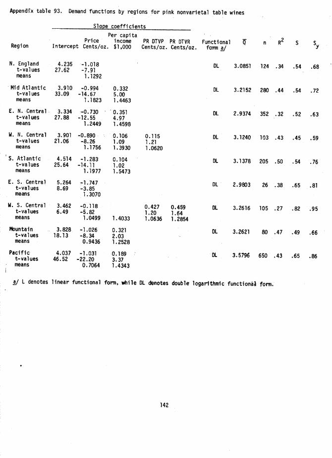
Appendix table 93. Demand functions by regions for pink nonvarietal table wines

Slope coefficients

Region Price

Intercept Cents/oz

Per capita Income

. $1.000 PR DTVP

Cents/oz. PR DTVR Cents/oz


4.235 27.62

-1.018 -7,91

1.1292


3.910 33.09

-0.994 -14.67

1.1823

0.332 5.00 1.4463


3.334 27.88

-0.730 -12.55

1.2449

0.351 4.97 1.4598


3.901 21.06

-0.890 -8,26

1.1756

0.106 1.09 1.3930

0.115 1.21 1.0620


4.514 25.64

-1.283 -14.11

1.1977

0.104 1.02 1.5473


5.264 8.69

-1.747 -3.85

1.3070


3.462 6.49

-0.118 -5.82

1.0499 1.4033

0.427 1.20 1.0636

0.459 1.64 1.2854


3.828 18.13

-1.026 -8.34 0,9436

0.321 2.03 1.2528

-


4.037 46.52

-1.031 -22,20

0.7064

0.189 i 3.37 1.4343

Functional foirm ñ/

DL 3.0851 124 .34 .54 .68

DL 3.2152 280 .44 .54 .72

DL 2.9374 352 .32 .52 .63

DL 3.1240 103 .43 .45 .59

DL 3.1378 205 .50 .54 .76

DL 2,9803 26 .38 .65 .81

DL 3.2616 105 .27 .82 .95

DL 3.2621 80 .47 .49 .66

DL 3.5796 650 .43 .65

a/ L denotes linear functional form, »hile DL denotes double logarithmic functional form.

142

Appendix table 94. Demand functions by regions for sherry dessert wines

Region Intercept

Per capita Price income PR DP0RT Functional

Cents/oz. $1,000 Cents/oz. forma/


3.619 13.80

-0.979 -6.56 1.2572

0.407 3.50 1.3779

DL 2.9482 97 .39 .60 .76


3.472 18.10

-0.642 -5.54 1.3596

0.228 3.37 1.4520

DL 2.9308 191 .18 .59 .65


2.697 15.72

-0.223 -2.39 1.368

0.165 1.76 1.485

DL 2.6368 133 .05 .45 .45


3.360 8.83

-0.752 -2.99

1.3167

0.261 1.57 1.3415

DL 2.720 35 .24 .48 .54


3.847 25.21

-0.752 -7.08 1.3923

DL 2.8003 179 .22 .51 .57


3.945 8.66

-1.007 -4.23 1.4706

0.256 1.42 1.3775

DL 2.817 43 .35 .47 .56


3.527 14.96

-0*645 -3.81 1.3541

DL 2.6529 94 .14 .52 .56


-15.692 -0.55

445 56 2561

1.676 1.60 4.8307

20.218 1.89 2.4820

24.8566 40 .28 14.47 16.42


2.489 12.05

288 66

1.1611

0.372 3.79 1.5104

DL 2.7171 212 .10 .65 .68


143

Appendix table 95. Demand functions by regions for port dessert wines

Slope coefficients

Region Intercept Price

Cents/oz,

Per capita Income

• $1,000 PR DSHRY Cents/oz,


4.074 13.52

-1.144 -5.95 1.1013

0.174 1.07 1.0764


4.527 24.6

-1.441 -8.78

1.1469

0.343 3.76 1.1950


3.968 19.00

-0.964 -5.90 1.2355


39.714 5.28

-4.316 -2,23 3.7216

-1.145 -1.05

3.0808

S. Atlantic t-values jneans

3.232 4.95

-0.993 -4.39 1.2738

0.832 1.87 1.2833

E. S. Central t*values means

1.978 3.01

-0.075 -0.21 1.4267

0.747 4.53 1.4860


3.830 11.19

-0.840 -3.78 1.2793

0.185 1.48 0.8331


44.066 6.28

-8.185 -4.03 2.8997

2.394 2.84 4.5664


8.556 1.31

-1.594 -1.97 3.1680

1.638 2.75 4.3136

2,416 1.23 3.1923

Functional form a/

DL 3.0007 57 .42 .57 .73

OL 3.2841 125 .39 .54 .68

DL 2.7771 73 .33 .45 ,55

L 20,124 30 .21 9.04 9.83

DL 3.035 53 .32 .52 .63

DL 2.9814 24 .55 .39 .55

DL 2.9095 45 .35 .53 .65

L 31.2625 40 .37 13.22 16.27

L 18.2821 88 .13 9.59 10.12

1/ L denotes linear functional form, while DL denotes double logarithmic functional form.

144

Appendix table 96. Demand functions by regions for apple flavored wines

Region

Slope coefficients Per capita

Price income Intercept Cents/oz. $1,000

Functional form a/


21.200 7.50

0.061 0.31 0.9929

0.392 2.37 1.1613


2.775 7,47

-0.495 -1.90 0.9825

0.383 2.18 1.1317


2.536 12.45

-0.321 -2.24

1.0138

0.360 3.73 1.3142


2.120 4.78

0.059 0.16 0.963

0.524 3.16 1.0626


3.172 14.39

-0.480 -2.62 1.1612


3.823 9.70

-0.833 -2.72

1.2358


2.194 6.01

0.158 0.59 1.0858

0.237 1.44 1.1418


2.892 7.36

-0.105 -0.26 0.9315


3.412 16.01

-0.376 -2.31 0.9516

-0.227 -1.57

1.2005

DL

DL

DL

DL

DL

DL

DL

DL

DL

2.6352

2.722

2.6843

2.7336

2.6152

2.7944

2.6367

2.7938

2.7816

20

36

86

29

55

17

30

15

73

.25

.25

.19

.29

.11

.33

.08

.01

.13

.38

.51

.44

.42

.42

.45

.47

.34

.55

.42

.57

.49

.48

.44

.53

.48

.33

.58


145

Appendix table 97. Demand functions by regions for berry flavored wines

Slope coefficients

Region intercept Price

Cents/oz.

Per capita income $1,000

Functional form a/

Q n

N, England t-values

3.007 7.58

-0.497 -1.62

0.216 1.15

DL 2.6831 25

means 1.1936 1.2456

Mid Atlantic t-values

2.643 14.30

-0.326 -2.71

0.366 4.18

DL 2.6826 69

means 1.2214 1.1986

E. N. Central t-values

2.557 14.38

-0.238 -1.91

0.303 4.15

DL 2.6326 143

means 1.2467 1.2279

W. N. Central t-values

21.371 3.86

-2.658 -2.29

1.751 1.26

L 18.1133 35

means 3.7027 3.7599

S, Atlantic t-values

2.932 9.87

-0.591 -3.47

0.266 2.54

DL 2.4597 50

means 1.3743 1.2794

-E. S. Central t-values

4.021 5.56

-1.110 1.95

DL 2.6546 11

means 1.2319

W. S. Central t-values

3.553 9.86

-0.764 -2.49

DL 2.6827 37

means 1.1401

Mountain t-values

3.742 7.89

-0.668 -1.93

DL 2.8499 20

means 1.3346

Pacific t-values

20.811 2.49

-2.523 -1.52

1.479 1.25

L 18.2377 60

means 3.4165 4.0916

R S S

.13 .39 .40

.27 .42 .48

.12 .46 .49

-14 10.48 11.00

.33 .35 .42

.30 .58 .6,6

.15 .52 .56

.17 .49 .53

.08 15.81 16.17


146

Appendix table 98. Demand functions by regions for citrus flavored wines

Slope coefficients


Cents/oz.

Per capita income $1.000

Functional form a/


2.143 3.51

-0.584 -1.71 1.3912

1.079 4.54 1.1920

DL


3.930 -1.120 1.2819

0.559 1.4207

DL


3.057 10.86

-0.702 -4.30

1.3323

0.445 3.65 1.3647

DL


means

3.954 14.12

-0.893 -4.37 1.3259

DL


3.598 9.64

-0.740 -3.59

1.5124

0.189 1.15 1.4803

DL


Too few observations


means

3.006 8.95

-0.873 -5.63

1.1706

0.539 3.18 1.3959

DL

Mountai n t-values means

4.155 18.18

-0.846 -4.11 0.9889

DL


3.762 17.77

-0.961 -10.59

1.TT79

0.133 1.13 1.4368

DL

2.6173

3.2876

2.7285

2.7696

2.7576

12

88

104

44

67

2.7368 27

3.3184 26

2.8780 109

.76

.41

.24

.31

.17

.68

.41

.53

.36

.60

.57

.47

.52

.66

.78

.64

.56

.56

.37 .63

.53 .68

,47 .68

hj L denotes linear functional form, while DL denotes doable logarithmic functional form.

147

Appendix table 99. Demand functions by regions for other flavored wines

Slope coefficients


Cents/oz.


Functional form bj

N. England t-va lues

3.899 19.06

-0.765 -4.52

DL

means 1.0982

Mid Atlantic t-values

3.672 16.62

-0.641 -4.06

0.120 1.70

DL

means 1.2602 1.1015

E. N. Central t-values

3.218 16.54

-0.682 -5.99

0.221 2.38

DL

means 1.1811 1.4809


3.350 11.05

-0.820 -5.79

0.265 1.49

DL

means 1.2377 1.3345

S. Atlantic t-values

3.418 10.16

-Ö.641 -2.90

0.240 1.62

DL

means 1.3059 1.2064

E. S. Central t-values

2.987 3.52

-0.145 -0.20

DL

means 1.1569


3.231 14.73

-0.302 -1.46

DL

means 0.9917

Mountain t-values

4.652 14.10

-0.956 -3.10

-0.374 -1.77

DL

means 0.875 0.9298

Pacific t-values

3.152 26.54

-0.249 -2.52

DL

means 1.0635

3.0589

2.9969

2.7417

2.6877

2.8710

2.8192

2.9315

3.4685

2.8870

26

65

114

47

47

13

37

26

77

R^ S

.46 .44

.24 .44

.27 .43

.45 .46

.19 .52

.004 .55

.06 .48

.39 .63

.08 .48

.58

.50

.50

.60

.56

.52

.49

,77

.50

a^/ L denotes linear functional form, while DL denotes double logarithmic functional for

148

Appendix table 100.. Demand functions by regions for sparkling champagne wines

Slope coefficients

Region Intercept

Per capita Price income

Cents/oz. $U000 Functional

form dj

N, England t-va lues means

3.264 7.81

-0,315 -1.38

1.7722

DL


2.977 6.80

-0.514 -2.67

1.8943

0.597 2.85 1.4250

DL


2.826 6.11

-0.405 -1.90

1.7584

0.527 3.00 1.5429

DL


2.378 2.30

-0.220 -0.37

1.8897

0.521 1.54 1.0258

DL


10.334 2.61

-0.649 -1.63 6.7339

2.123 3.27 4.6036

L

E. S. Central Too few observations t-values means


2.952 3.28

0.122 0.23 1.7195

DL

Mountain Too few observations t-values means


2.897 8.01

-0.532 -3.74 1.6738

0.613 3.26 1.5564

DL

2.7059

2.8541

2.9257

2.4961

15.7332

19

92

78

13

56

3.1624 27

R S S..

.10 .44 .45

.13 .83 .87

.14 .69 .74

.20 .50 .51

.19 8.38 9.13

.002 .95 .93

2.9605 82 .22 .63 .70

hj L denotes linear functional form, while DL denotes double logarithmic functional form.

149

Appendix table 101. Demand functions by regions for sparkling burgundy wines

Region

Slope coefficients

Intercept

Per capita Price income PR OSPCH Functional

Gents/oz. $1,000 Gervts/oz. forma/


ma Atlantic t-values means

3.729 5.03

2,857 3.09

-0.501 -2.09 1.9867

-0/361 -0.77 1.8532

-0.673 -1.83 1.1701

0.393 1.15 1.4197

0.399 2.10 1.6500

DL 2.6062 9 .73 .29 .45

DL 2.7456 15 .12 .52 .52

E, N. Central t-values means

2.714 5.33

136 44 5973

DL 2,9309 20 .01 .58 .57

W. N. Gentral t-values means

17.521 5.02

-1.0918 -1.63 5.0223

12.0381 7 .35 2.36 2.66


4.656 10.03

■1.087 -3.37 1.3544

DL 3.1848 11 .56 ;52 .74

E, S. Central t-values means




2.920 -0.008 2.88 -0.02

1.8262


DL 2,9044 7 .0001 ,91 .83




150

Appendix table 102. Demand functions by regions for sparkling cold duck wines

Region

Slope coefficients

Intercept Price

Cents/oz


PR DSPCH Cents/oz.

Functional form a^/







: W. S. Central t-values means



1.986 2.50

3.561 8.11

3.673 13.45

2.449 2.43

3.258 7,23

3.924 3.21

3.040 4.23

4.827 4.27

2.314 3.67

-0.484 -1.24

1.6775

-0.814 -3.49

1.6441

-0.548 -3.42

1.6597

-0.363 -0.84

1.6930

-0.438 -1.76

1.7274

-0.784 -1.26

1.9401

-0.579 -1.55

1.6888

-1.157 -1.61 1.5647

0.298 0.78 1.6429

0.475 1.92 1.0358

0.379 2.36 1.3890

0.617 1.95 1.3202

0.200 1.20 1.5374

0.401 1.66 1.3416

0.600 2.28 1.8713

DL 2.7897 20 .32 .57 .64

DL 2.7495 63 .22 .59 .66

DL 2.7643 66 .15 .52 .56

DL 2.6484 27 .25 .59 .65

DL 2.8082 41 .09 .46 .47

DL 2.4035 12 .14 .55 .56

DL 2.5998 28 .17 .56 .59

DL 3.0168 14 .18 .54 .57

DL 2.8032 38 .02 .55 .55

a/ L denotes linear functional form, while DL denotes double logarithmic form.

151

Appendix table 103. Demand functions by regions for vermouth wines

Slope coefficients


Cents/o2

Per capita income

. $1,000 PR IVER

Cents/oz


4.034 17.49

-1.042 -9.13

1.0421

0.125 1.06 1.3124


4.315 16.52

-1.080 -5.04

1.1690


1.969 3.07

-0.306 -1.53

1.4018

0.171 1.70 1.5127

0.422 1.33 1.9050




3.525 6.33

-1.042 -4.27

1.3458

-0.163 -1.96 1.3532

0.428 1.96 1.9687


20.298 1.93

-1.481 -0,60 4.1985



ftountain t-values means

24.278 1.61

-3.925 -0.68 2.5980


17,449 7.18

-1.530 -2.14 3.3058

Functional Q n R S S form a/ y

DL 3.1126 15 .89 .23 .66

DL 3.0521 61 .30 .59 .69

DL 2.6027 51 .11 ,33 .33

DL 2.7437 30 .54 .27 .38

L 14.0800 10 .04 4.20 4.05

L 14.0800 10 .05 4.17 4.05

L 12,3914 47 .09 4.07 4.22


152

* Ü,S. OOVERMENT PIŒMTIN6 OFFICE, s 1978 0-280-93l/ESCS-2

THE U.S. WINE MARKET

Documents

Transcript of THE U.S. WINE MARKET