The University of

Ontario

CS 4487/9587

Algorithms for Image Analysis

Image Modalitiesmost slides are shamelessly stolen from Steven Seitz, Aleosha Efros, and Terry Peters

The University of

Ontario

CS 4487/9587 Algorithms for Image Analysis Image Modalities

Photo/Video data• Pin-hole• Lenses• Digital images and volumes

Medical Images and Volumes• X-ray, MRI, CT, and Ultrasound

Extra Reading: Forsyth & Ponce, Ch. 1. Gonzalez & Woods, Ch. 1

The University of

Ontario

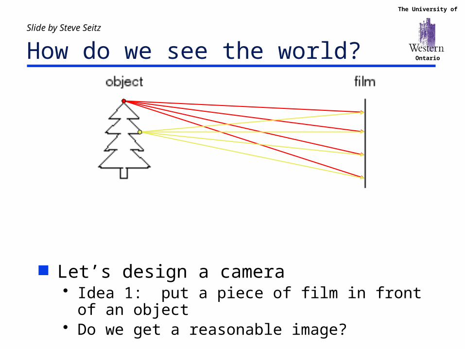
Slide by Steve Seitz How do we see the world?

Let’s design a camera• Idea 1: put a piece of film in front of an object• Do we get a reasonable image?

The University of

Ontario

Slide by Steve Seitz Pinhole camera

Add a barrier to block off most of the rays• This reduces blurring• The opening known as the aperture• How does this transform the image?

The University of

Ontario

Slide by Steve Seitz Camera Obscura

The first camera• Known to Aristotle• Depth of the room is the focal length• Pencil of rays – all rays through a point• Can we measure distances?

The University of

Ontario

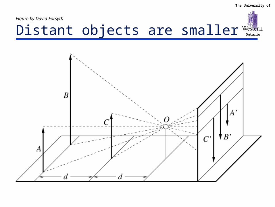
Figure by David Forsyth

Distant objects are smaller

The University of

Ontario

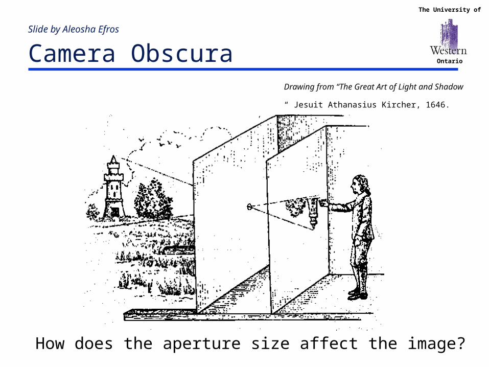
Slide by Aleosha Efros Camera Obscura

Drawing from “The Great Art of Light and Shadow “

Jesuit Athanasius Kircher, 1646.

How does the aperture size affect the image?

The University of

Ontario

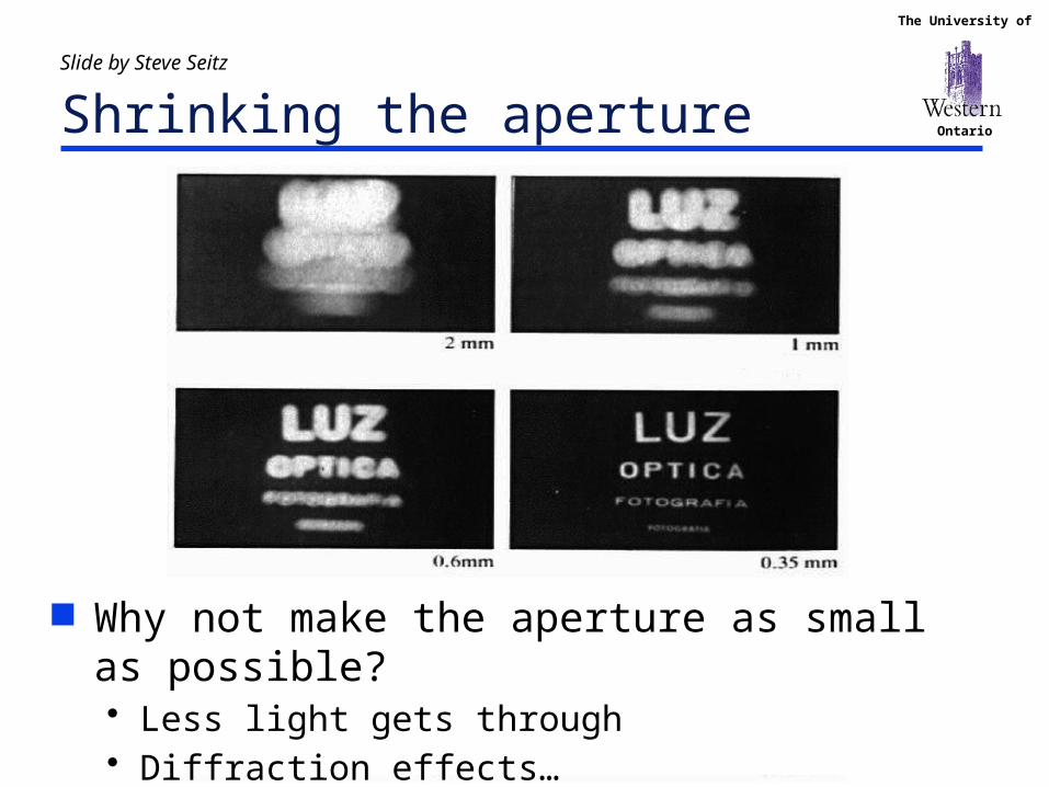
Slide by Steve Seitz Shrinking the aperture

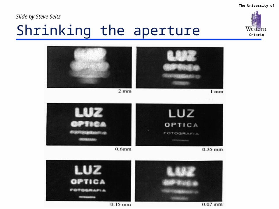
Why not make the aperture as small as possible?• Less light gets through• Diffraction effects…

The University of

Ontario

Slide by Steve Seitz Shrinking the aperture

The University of

Ontario

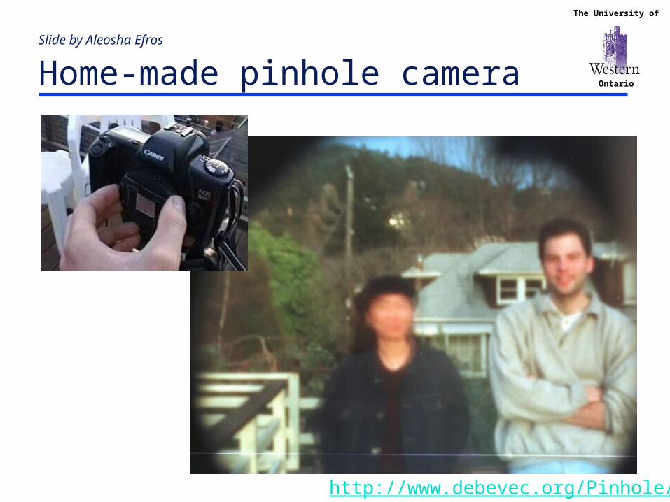
Slide by Aleosha Efros Home-made pinhole camera

http://www.debevec.org/Pinhole/

The University of

Ontario

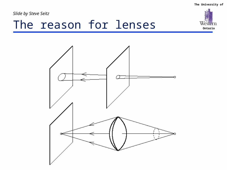
Slide by Steve Seitz The reason for lenses

The University of

Ontario

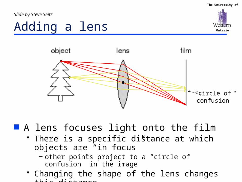
Slide by Steve Seitz Adding a lens

A lens focuses light onto the film• There is a specific distance at which objects are “in focus”

– other points project to a “circle of confusion” in the image• Changing the shape of the lens changes this distance

“circle of confusion”

The University of

Ontario

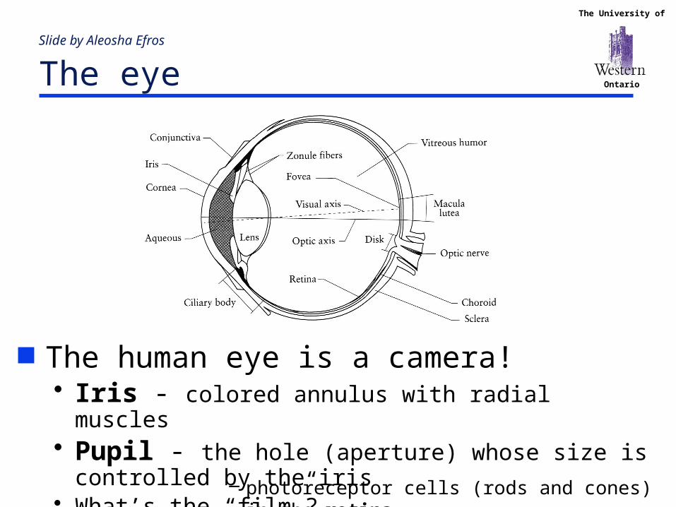
Slide by Aleosha Efros The eye

The human eye is a camera!• Iris - colored annulus with radial muscles• Pupil - the hole (aperture) whose size is controlled by the iris• What’s the “film”?

– photoreceptor cells (rods and cones) in the retina

The University of

Ontario

Slide by Aleosha Efros Cameras

Really cool Not too expensive nowadays (<$200)

Canon A70

The University of

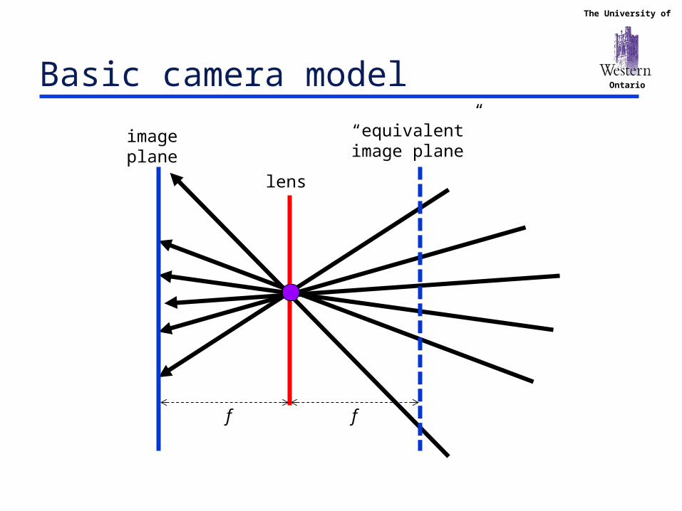
OntarioBasic camera model

image plane

lens

f

“equivalent” image plane

f

The University of

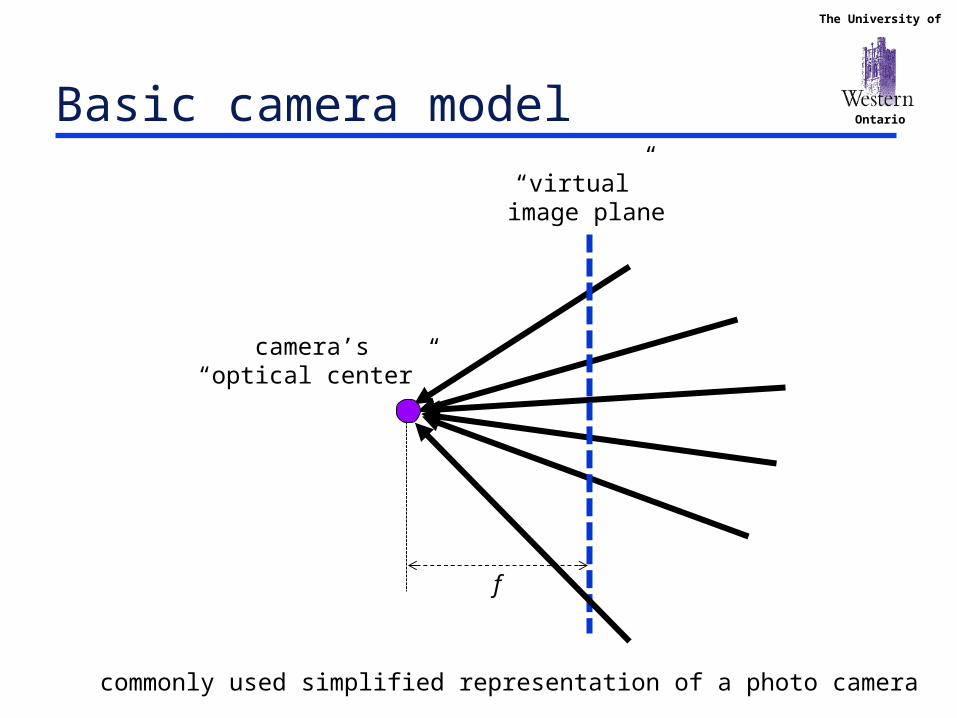
OntarioBasic camera model

“virtual” image plane

camera’s“optical center”

f

commonly used simplified representation of a photo camera

The University of

Ontario

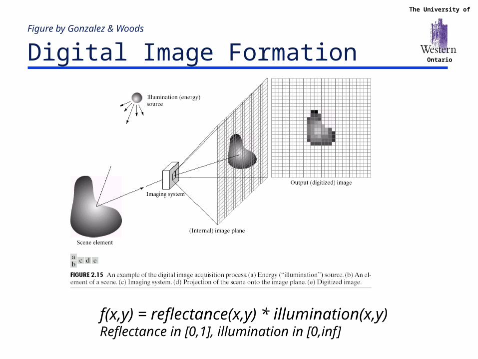
Figure by Gonzalez & Woods Digital Image Formation

f(x,y) = reflectance(x,y) * illumination(x,y)Reflectance in [0,1], illumination in [0,inf]

The University of

Ontario

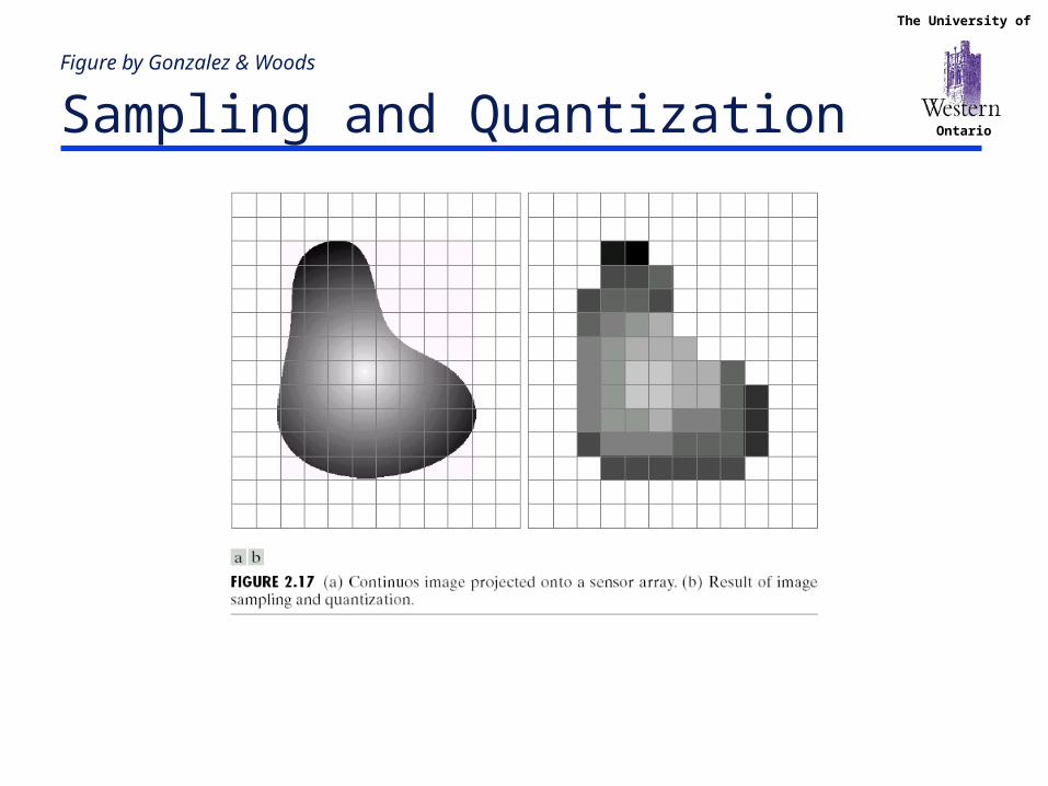
Figure by Gonzalez & Woods Sampling and Quantization

The University of

Ontario

Figure by Gonzalez & Woods Sampling and Quantization

The University of

Ontario

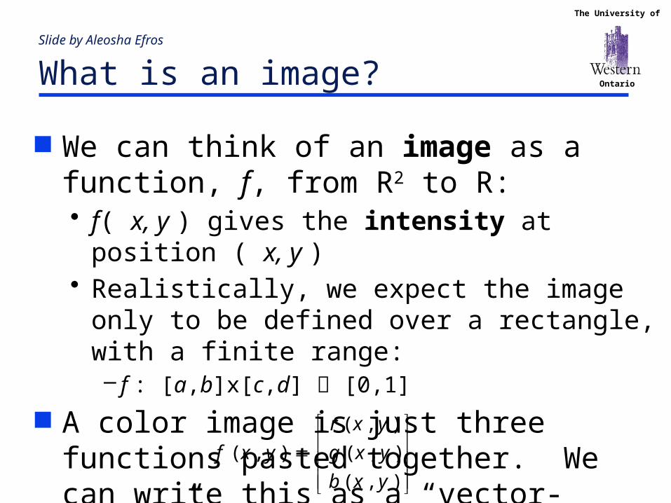
Slide by Aleosha Efros What is an image?

We can think of an image as a function, f, from R2 to R:• f( x, y ) gives the intensity at position ( x, y ) • Realistically, we expect the image only to be defined

over a rectangle, with a finite range:– f : [a,b]x[c,d] [0,1]

A color image is just three functions pasted together. We can write this as a “vector-valued” function: ( , )

( , ) ( , )

( , )

r x y

f x y g x y

b x y

The University of

Ontario

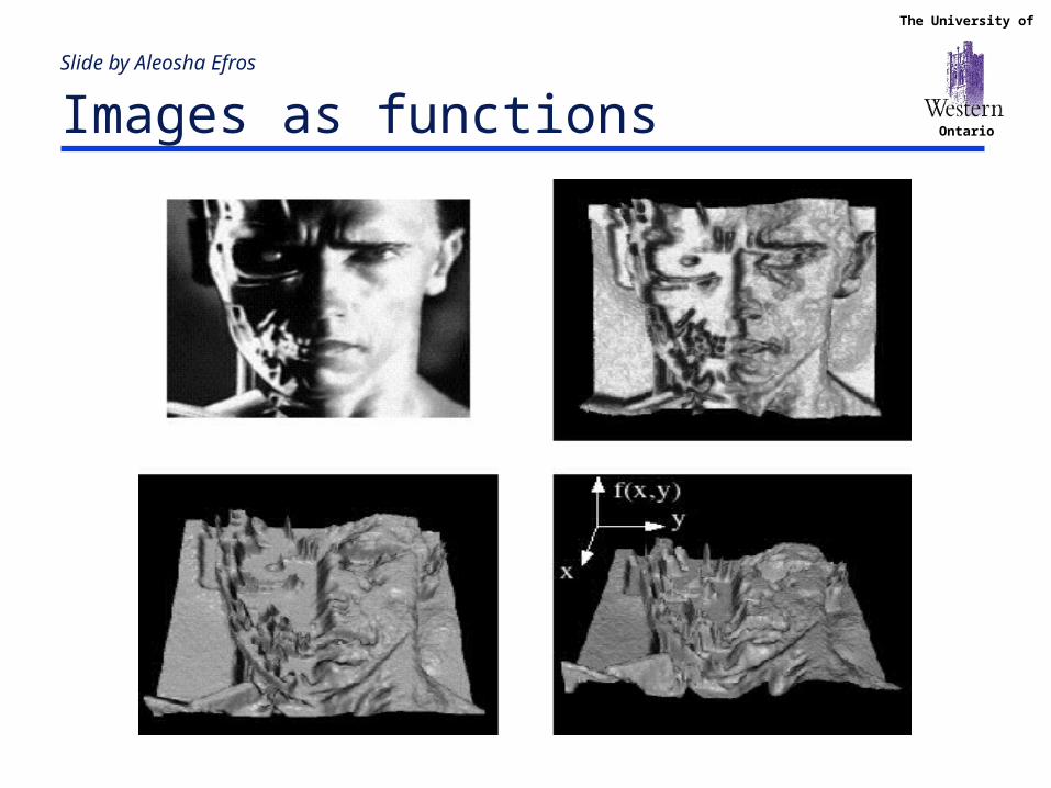
Slide by Aleosha Efros Images as functions

The University of

Ontario

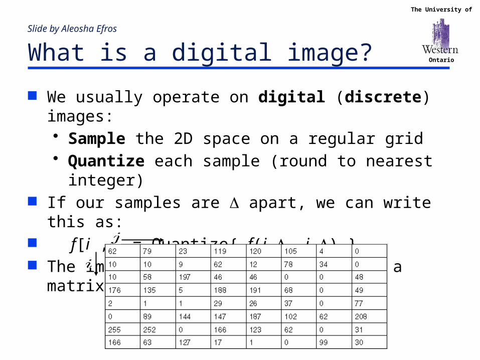
Slide by Aleosha Efros What is a digital image?

We usually operate on digital (discrete) images:• Sample the 2D space on a regular grid• Quantize each sample (round to nearest integer)

If our samples are D apart, we can write this as: f[i ,j] = Quantize{ f(i D, j D) } The image can now be represented as a matrix of integer values

The University of

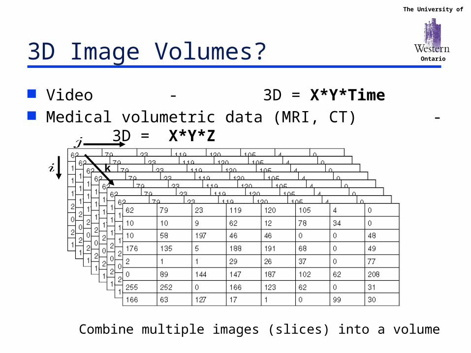
Ontario3D Image Volumes?

Video - 3D = X*Y*Time Medical volumetric data (MRI, CT) - 3D = X*Y*Z

k

Combine multiple images (slices) into a volume

The University of

Ontario

CS 4487/9587 Algorithms for Image Analysis Image Modalities

• X-ray• CT • MRI• Ultrasound

PART II: Medical images and volumes

The University of

Ontario

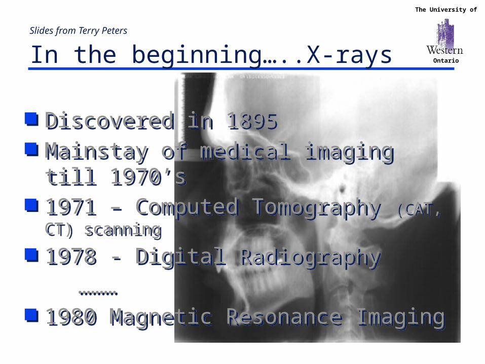
Slides from Terry Peters In the beginning…..X-rays

Discovered in 1895 Mainstay of medical imaging till 1970’s 1971 – Computed Tomography (CAT, CT) scanning

1978 - Digital Radiography

……… 1980 Magnetic Resonance Imaging

Discovered in 1895 Mainstay of medical imaging till 1970’s 1971 – Computed Tomography (CAT, CT) scanning

1978 - Digital Radiography

……… 1980 Magnetic Resonance Imaging

The University of

OntarioX-rays

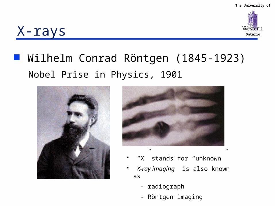
Wilhelm Conrad Röntgen (1845-1923)

Nobel Prise in Physics, 1901

• “X” stands for “unknown”

• X-ray imaging is also known as

- radiograph

- Röntgen imaging

The University of

OntarioX-rays

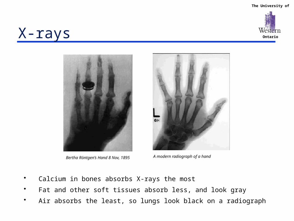
Bertha Röntgen’s Hand 8 Nov, 1895 A modern radiograph of a hand

• Calcium in bones absorbs X-rays the most

• Fat and other soft tissues absorb less, and look gray

• Air absorbs the least, so lungs look black on a radiograph

The University of

OntarioX-rays

2D “projection” imaging 1895 - 1970’s

The University of

Ontario

From Projection ImagingTowards True 3D Imaging

Mathematical results: Radon transformation

1917

Computers can perform complex mathematics to

reconstruct and process imagesLate 1960’s:

X-ray imaging1895

Development of CT (computed tomography) 1972

• Image reconstruction from projection

• Also known as CAT (Computerized Axial Tomography)

• "tomos" means "slice" (Greek)

The University of

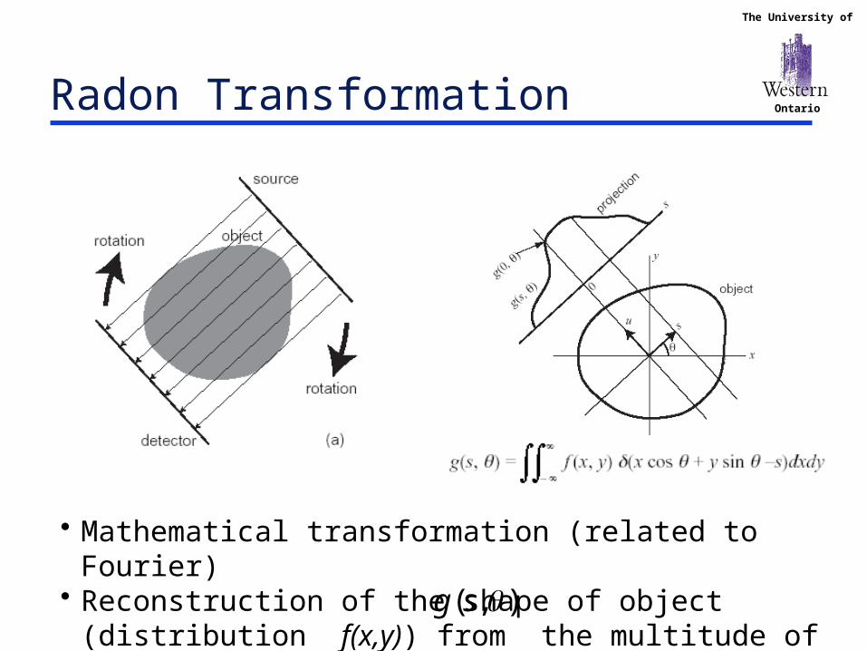
OntarioRadon Transformation

• Mathematical transformation (related to Fourier) • Reconstruction of the shape of object (distribution f(x,y)) from

the multitude of 2D projections ),( sg

The University of

Ontario

Figure from www.imaginis.com/ct-scan/how_ct.asp

CT imaging

The University of

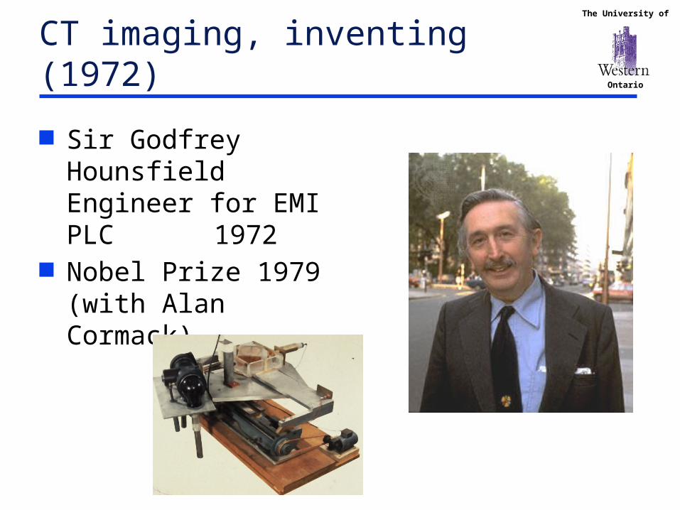
OntarioCT imaging, inventing (1972)

Sir Godfrey Hounsfield Engineer for EMI PLC

1972 Nobel Prize 1979 (with

Alan Cormack)

The University of

OntarioCT imaging, availability (since 1975)

The EMI-ScannerOriginal axial CT image from the dedicated Siretom CT scanner circa 1975. This image is a coarse 128 x 128 matrix; however, in 1975 physicians were fascinated by the ability to see the soft tissue structures of the brain, including the black ventricles for the first time (enlarged in this patient)

1974

Axial CT image of a normal brain using a state-of-the-art CT system and a 512 x 512 matrix image. Note the two black "pea-shaped" ventricles in the middle of the brain and the subtle delineation of gray and white matter(Courtesy: Siemens)

25 years later

The University of

Ontario

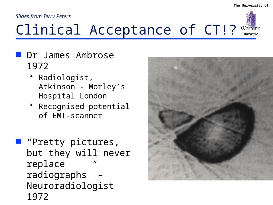
Slides from Terry Peters Clinical Acceptance of CT!?

Dr James Ambrose 1972• Radiologist, Atkinson -

Morley’s Hospital London• Recognised potential of EMI-

scanner

“Pretty pictures, but they will never replace radiographs” –Neuroradiologist 1972

The University of

Ontario

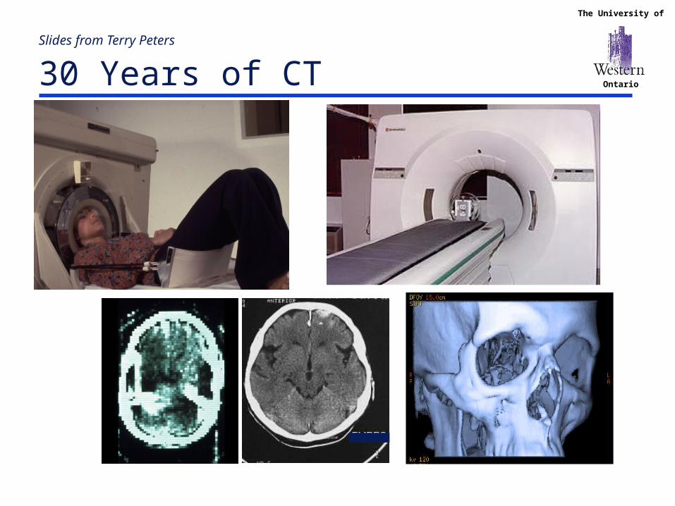
Slides from Terry Peters Then ……………and Now

80 x 80 image 3 mm pixels 13 mm thick slices Two simultaneous

slices!!! 80 sec scan time per

slice 80 sec recon time

512 x 512 image <1mm slice thickness <0.5mm pixels 0.5 sec rotation 0.5 sec recon per slice Isotropic resolution Spiral scanning - up to

16 slices simultaneously

The University of

Ontario

Slides from Terry Peters 30 Years of CT

The University of

Ontario

Slides from Terry Peters Birth of MRI

Paul Lautebur 1975• Presented at Stanford CT

meeting• “Zeugmatography”

Raymond Damadian 1977 – Sir Peter Mansfield early

1980’s

Early Thorax Image Nottingham

The University of

Ontario

Slides from Terry Peters Birth of MRI

Early Thorax Image Nottingham

• Electro Marnetic signal emitted (in harmless radio frequensy) is acquired in the time domain • image has to be reconstructed (Fourier transform)

The University of

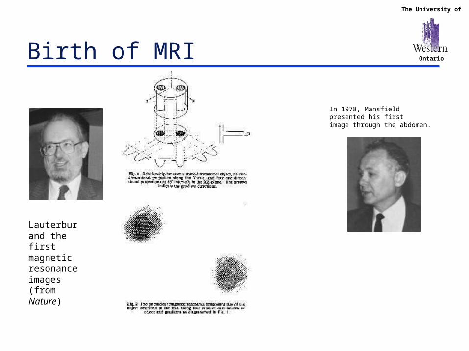
OntarioBirth of MRI

In 1978, Mansfield presented his first image through the abdomen.

Lauterbur and the first magnetic resonance images (from Nature)

The University of

Ontario

Slides from Terry Peters 30 Years of MRI

First brain MR image Typical T2-weighted MR image

The University of

Ontario

Slides from Terry Peters MR Imaging

“Interesting images, but will never be as useful as CT”

• (A different) neuroradiologist, 1982

The University of

Ontario

Slides from Terry Peters MR Imaging …more than T1 and T2

MRA - Magnetic resonance angiography• images of vessels

MRS - Magnetic resonance spectroscopy• images of chemistry of the brain and muscle metabolism

fMRI - functional magnetic resonance imaging• image of brain function

PW MRI – Perfusion-weighted imaging DW MRI – Diffusion-weighted MRI

• images of nerve pathways

The University of

Ontario

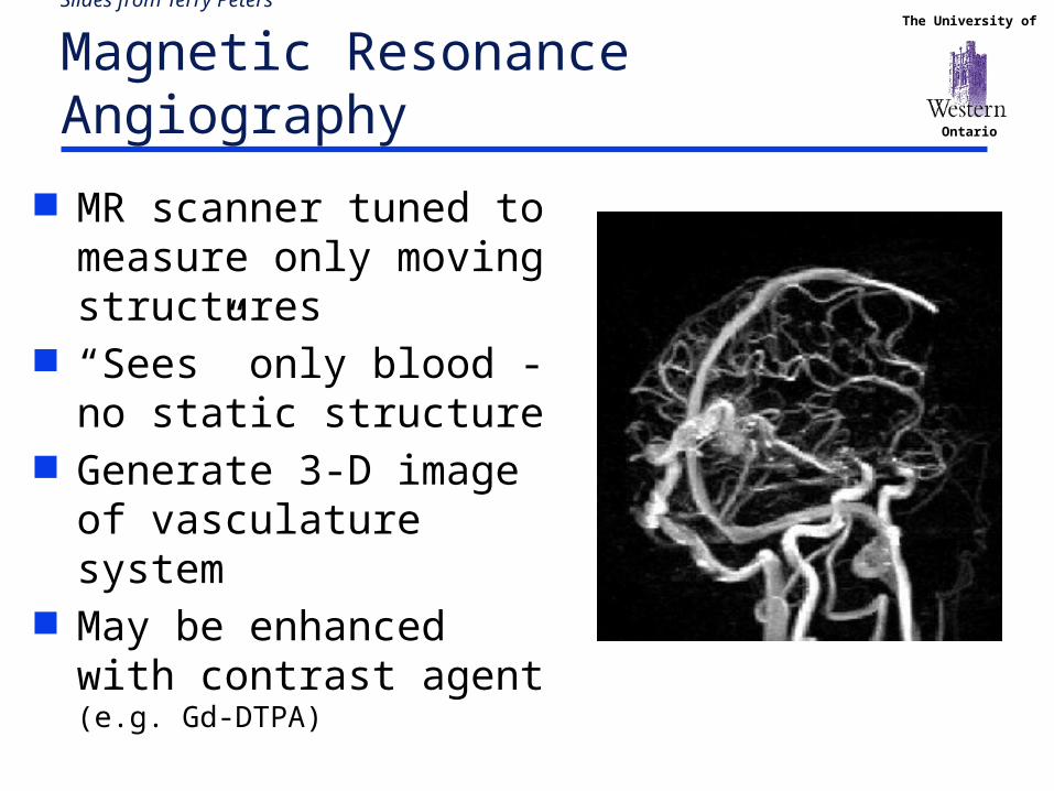
Slides from Terry Peters Magnetic Resonance Angiography

MR scanner tuned to measure only moving structures

“Sees” only blood - no static structure

Generate 3-D image of vasculature system

May be enhanced with contrast agent (e.g. Gd-DTPA)

The University of

Ontario

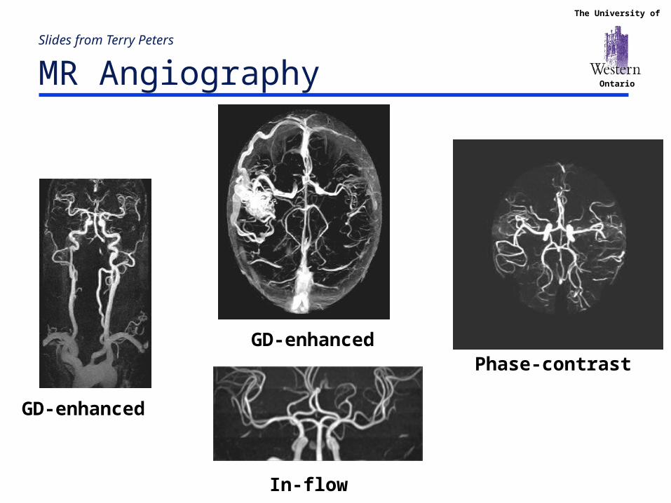
Slides from Terry Peters MR Angiography

Phase-contrast

In-flow

GD-enhanced

GD-enhanced

The University of

Ontario

1 www.atamai.com

Slides from Terry Peters

Dynamic 3-D MRI of the thorax

The University of

Ontario

Slides from Terry Peters Diffusion-Weighted MRI

Image diffuse fluid motion in brain

Construct “Tensor image” – extent of diffusion in each direction in each voxel in image

Diffusion along nerve sheaths defines nerve tracts.

Create images of nerve connections/pathways

The University of

Ontario

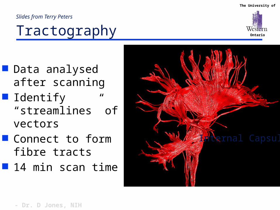
Data analysed after scanning

Identify “streamlines” of vectors

Connect to form fibre tracts

14 min scan time

- Dr. D Jones, NIH

Internal Capsule

Slides from Terry Peters Tractography

The University of

Ontario

Slides from Terry Peters Tractography

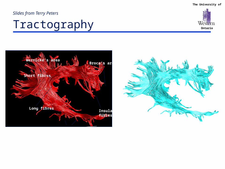
Superior

Longitudinal Fasciculus

Short fibres

Temporal fibres

Insula fibres

Wernicke’s areaBroca’s area

Long fibres

- Dr. D Jones, NIH USA

“just like Gray’s Anatomy”!

The University of

Ontario

Slides from Terry Peters Functional MRI (fMRI)

Active brain regions demand more fuel (oxygen)

Extra oxygen in blood changes MRI signal Activate brain regions with specific tasks Oxygenated blood generates small (~1%) signal

change Correlate signal intensity change with task Represent changes on anatomical images

The University of

Ontario

Slides from Terry Peters fMRI

Subject looks at flashing disk while being scanned“Activated” sites detected and merged with 3-D MR image

Stimulus

Activation

The University of

Ontario

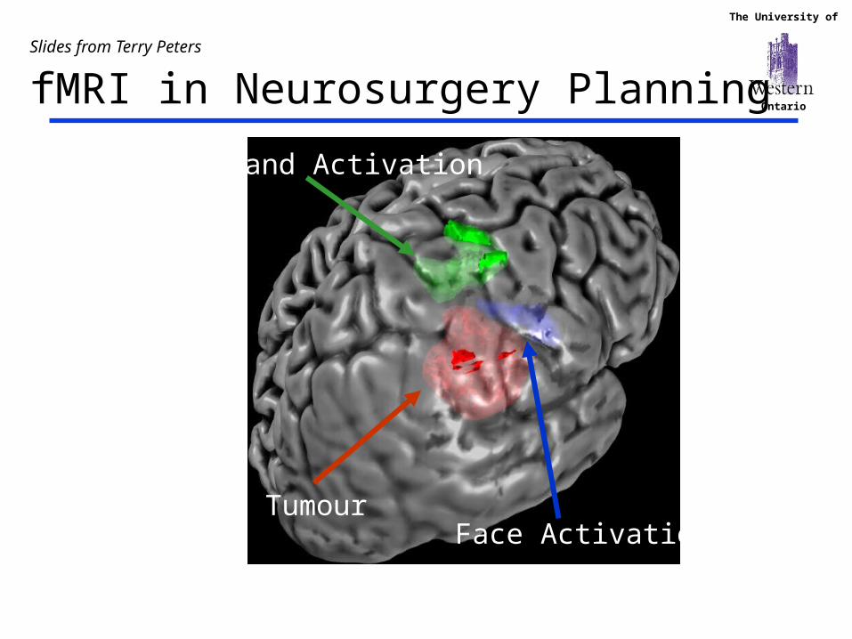
Hand Activation

Face ActivationTumour

Slides from Terry Peters fMRI in Neurosurgery Planning

The University of

Ontario

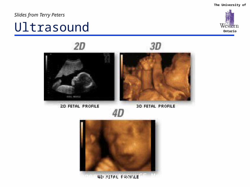
Slides from Terry Peters Ultrasound

Images courtesy GE Medical