THE UNIVERSITY OF CHICAGO

CONSTRUCTION, IMPLEMENTATION, AND THEORY

OF ALGORITHMS BASED ON

DATA AUGMENTATION AND MODEL REDUCTION

A DISSERTATION SUBMITTED TO

THE FACULTY OF THE DIVISION OF THE PHYSICAL SCIENCES

IN CANDIDACY FOR THE DEGREE OF

DOCTOR OF PHILOSOPHY

DEPARTMENT OF STATISTICS

BY

DAVID ANTHONY VAN DYK

CHICAGO, ILLINOIS

AUGUST 1995

Acknowledgements

I wish to thank my advisor, Xiao-Li Meng, for his unending support as I

completed this project. He is a gifted and patient teacher who never failed to

make time to answer my questions, to point me in the direction of interesting and

fruitful research topics, or to think carefully and critically about my work. I am

very appreciative of his willingness to go far beyond the call of duty.

There are many others who have helped greatly in the completion of this

thesis. Here I can mention only a few, but would like to thank Don Rubin for

his help with Chapter 4, Augustine Kong for helping me obtain two summers of

research support, Jeffrey Fessler for comments pertaining to the SAGE algorithm

and Chapter 5, Sam Vandervelde for his never-ending willingness to help me with

the subtler details of the mathematics underlying my work, and Ron Thisted for

comments on presentation and pointing out several helpful references.

This work was supported in part by National Science Foundation grant

DMS 89-05292, the Department of Education (through GAANN program awards

P200A10027 and P200A40313), the U.S. Public Health Service/National Institutes

of Health (PHS/NIH GM 46800), The University of Chicago Louis Block Fund,

and the U.S. Census Bureau through a contract with the National Opinion Re-

search Center at the University of Chicago. Computations for this document were

performed using computer facilities supported in part by the National Science Foun-

dation under grants DMS 89-05292 and DMS 87-03942 awarded to the Department

of Statistics at The University of Chicago, and by The University of Chicago Block

Fund. I am grateful to all of these sources for their financial support.

Finally, I wish to thank Greg Jao and Peter Vassilatos for their many editorial

comments.

Abstract

In the thesis we provide a general framework for maximum likelihood al-

gorithms based on data augmentation and model reduction. Starting with this

theoretical framework, we explore methods of constructing and implementing effi-

cient algorithms. We show how to derive faster algorithms by optimizing the rate of

convergence as a function of a working parameter which is introduced into the data-

augmentation scheme. We then propose the Alternating Expectation/Conditional

Maximization or AECM algorithm which includes the EM, ECM, ECME, and

SAGE algorithms as special cases. We also show how the matrix rate of convergence

can be used to compute the asymptotic variance-covariance matrix of the maximum

likelihood estimates. The relative efficiency of competing model-reduction schemes

is explored via permutation of the conditional maximization steps within the ECM

algorithm. Finally, we explore the inferential use of the data-augmentation scheme

in the context of estimating the number of components in a finite mixture, with

possible extensions to other model-fitting problems.

Chapter 1

EM-type Algorithms:

Background and Notation

1.1. A Brief Overview

The Expectation/Maximization or EM algorithm (Dempster, Laird, and Rubin,

1977) is a formalization of an old ad hoc method for handling missing data. If we

had observed the missing values, we could estimate the parameters of a posited

model using standard complete-data techniques. On the other hand, if we knew the

model parameters, we could impute the missing data according to the model. This

leads naturally to an iterative scheme. The advantage of the EM formulation over

its ad hoc predecessor is that it recognizes that the correct imputation is through

the complete-data sufficient statistics, or more generally through the complete-data

loglikelihood function, and not the individual missing values. Specifically, at each

iteration the E-step computes the conditional expectation of the complete-data log-

likelihood given the observed data and the previous iterate of the parameter value,

and the M-step then maximizes this imputed loglikelihood function to determine

1

2

the next iterate of the parameter. We repeat this process until the algorithm con-

verges. Since EM separates the complete-data analysis from the extra complications

due to missing data and allows the use of complete-data maximization techniques,

it is both conceptually and computationally simple. When facing an incomplete-

data problem, we can first ask what would be done if there were no missing values,

and then proceed with the help of EM to deal with the missing data, assuming

that the missing-data mechanism (Rubin, 1976) has been taken into account. This

advantage has helped EM win great popularity among practical users. Meng and

Pedlow’s (1992) bibliography reveals that there are more than 1,000 EM-related

articles in almost 300 journals, most of which are outside the field of statistics.

1.1.1. Model reduction

In some cases, the complete-data problem itself may be complicated. For instance,

when a model has many parameters, finding maximum likelihood estimates (MLEs)

can be a demanding task. A natural strategy, in general, is to break a big problem

into several smaller ones. If some of the model parameters were known, it might

be easier to estimate the rest. In the complete-data problem, we can partition the

parameters into several sets and estimate one set conditional on all the others. This

model-reduction technique is well-known in the numerical analysis literature as the

cyclic coordinate ascent method (e.g. Zangwill, 1969) and is called in statistical

terms the Conditional Maximization or CM algorithm by Meng and Rubin (1993),

whose model-reduction scheme goes beyond a simple partition of the parameter, as

they find a more sophisticated model-reduction scheme is useful for certain statisti-

3

cal models. The Expectation/Conditional Maximization or ECM algorithm (Meng

and Rubin, 1993) is an efficient combination of the CM and EM algorithms. It

replaces the maximization step of EM with a set of conditional maximization steps,

and thus splits a difficult maximization problem into several easier ones. Conse-

quently, in many practical applications, the use of model reduction in ECM extends

the flexibility and power of EM while retaining its stability in the sense of monotonic

convergence of the likelihood along the induced sequence to the MLE. The flexi-

bility introduced by model reduction also allows more efficient data-augmentation

schemes, as we shall explore in this thesis.

1.1.2. Data-augmentation

Although the principal reasons for the popularity of EM and ECM are their sim-

plicity and stability, they are sometimes criticized because of their slow convergence

in some applications. Loosely speaking, the rate of convergence is governed by the

amount of missing information in terms of the observed Fisher information. The

more missing information, the slower the algorithms will converge. Although EM is

motivated by the idea of a missing-data structure, in many of its novel applications,

there is strictly speaking no missing data in the usual sense. That is, the observed

data is simply augmented to some larger data set for which analysis is simpler (for

this reason, in what follows we will use the more general term “augmented data”

in place of “complete data”). Choosing a sensible data-augmentation scheme is an

art which requires compromising between simplicity (which often means more aug-

mentation) and fast convergence (which often requires less augmentation). Thus,

4

careful selection of the data-augmentation scheme can lead to simpler and faster al-

gorithms. Good examples of careful selection include, the Expectation/Conditional

Maximization Either or ECME algorithm (Liu and Rubin, 1995a) and the Space-

Alternating Generalized EM or SAGE algorithm (Fessler and Hero, 1994), both of

which are extensions of the ECM algorithm. Both algorithms incorporate effective

data-augmentation schemes to improve the rate of convergence of the algorithm. A

primary contribution of this thesis is to illustrate a new technique for the construc-

tion of effective data-augmentation schemes, which leads to algorithms that not

only maintain the simplicity and stability of the EM algorithm but also substan-

tially improve upon its rate of convergence. In the problems we consider, the new

algorithms are often ten times or even hundreds of times faster than their standard

counterparts in terms of actual computation time.

1.1.3. Synopsis

In what follows, we will explore methods of constructing, implementing, and ana-

lyzing algorithms which incorporate both model-reduction and effective data aug-

mentation into the EM algorithm. Our exploration also illustrates the theoretical,

computational, and inferential use of the rate of convergence of EM-type algo-

rithms. Chapter 2 focuses on constructing optimal algorithms in terms of their

rate of convergence via the introduction of a working parameter indexing a class of

data-augmentation schemes. As we will see, this leads to simple changes in some

standard algorithms and results in dramatic increases in computational efficiency.

In Chapter 3 we will develop the Alternating Expectation/Conditional Maximiza-

5

tion or AECM algorithm, a generalization of EM which incorporates both model

reduction to simplify implementation and a scheme that allows the data augmenta-

tion to be altered at each iteration to improve the overall rate of convergence of the

algorithm. AECM will be shown to include not only EM, ECM, and SAGE but also

the soon-to-be-discussed PECM and MCECM algorithms (Meng and Rubin, 1993)

as well as the special case of ECME for which Liu and Rubin’s (1995a) convergence

theorems hold; we will discuss why their general theory applies only to this special

case.

All of these algorithms are designed to calculate maximum likelihood esti-

mates or posterior modes. In most statistical analysis, however, measures of uncer-

tainty (e.g., asymptotic variance-covariance matrix of the estimates) are also needed.

Chapter 4 develops the Supplemented ECM or SECM algorithm which is designed

to do this when implementing ECM and which can be used in most implementations

of the AECM algorithm. As we have seen, we incorporate model reduction into EM

by breaking the maximization step into several conditional maximization steps. The

order that these steps are performed is trivial to change but generally affects the

performance of the algorithm (e.g., rate of convergence). Chapter 5 thus explores

the effect of permutation of conditional maximization steps in the context of ECM

and illustrates several valuable lessons pertaining to the incongruence of empirical

and theoretical results that will have implications in other studies. Finally, Chap-

ter 6 looks at the inferential use of the data-augmentation scheme through the rate

of convergence of EM in the context of estimating the number of components in a

finite mixture, with possible extensions to other model fitting problems.

6

The remainder of the current chapter outlines the details and notation of

the EM, ECM, ECME and SAGE algorithms, as well as the theory of the rate of

convergence of EM-type algorithms, thereby explicitly illustrating model reduction

and data augmentation in EM-type algorithms.

1.2. The EM Algorithm

Let L(θ|Yobs) = log f(Yobs|θ) be the observed-data loglikelihood function that we

want to maximize, where θ = (θ1, . . . , θd) is a d -dimensional model parameter

with domain Θ . (For simplicity, we assume this model already has incorporated

any non-ignorable missing-data mechanism; see Rubin, 1976.) Let f(Yaug|θ) be

a density for the augmented data Yaug = (Yobs, Ymis) , where Ymis is the missing

(i.e., unobserved) part. The augmented data are chosen such that maximizing

L(θ|Yaug) = log f(Yaug|θ) is much easier than directly maximizing L(θ|Yobs) . This

is the setting in which EM and its extensions are most useful.

Starting with an initial value θ(0) ∈ Θ , the EM algorithm finds θ⋆ , a maxi-

mizer of L(θ|Yobs) , by iterating the following two steps (t = 0, 1, . . .) :

E-step: Impute the unknown augmented-data loglikelihood L(θ|Yaug) by its

conditional expectation given Yobs and the current estimate θ(t) :

Q(θ|θ(t)) =

∫L(θ|Yaug)f(Ymis|Yobs, θ

(t))dYmis. (1.2.1)

7

M-step: Determine θ(t+1) by maximizing the imputed loglikelihood Q(θ|θ(t)) :

Q(θ(t+1)|θ(t)) ≥ Q(θ|θ(t)), for all θ ∈ Θ. (1.2.2)

For exponential families, Q(θ|θ(t)) = L(θ|S(t)(Yobs)) , where S(t)(Yobs) =

E[S(Yaug)|Yobs, θ(t)] with S(Yaug) being the augmented-data (vector) sufficient

statistic. The E-step therefore reduces to finding the conditional expectation of

S(Yaug) , and maximizing Q(θ|θ(t)) is computationally the same as maximizing

L(θ|Yaug) , the augmented-data loglikelihood. The latter is one of the principal

reasons for the popularity of the EM algorithm in practice because it allows prac-

titioners to use existing (complete-data) techniques and software when Yaug is

properly chosen.

The convergence properties of EM were established by Dempster, Laird, and

Rubin (1977) and Wu (1983). In particular, EM is a GEM (Generalized EM)

which ensures that L(θ(t+1)|Yobs) ≥ L(θ(t)|Yobs) for any sequence {θ(t) : t ≥

0} of EM iterates. Moreover, given mild regularity conditions, it can be shown

that EM converges to a stationary point (typically a local mode in practice) of

L(θ|Yobs) . These stability properties combined with simple implementation are

very attractive to analysts who are not necessarily numerically sophisticated and

whose main objectives are not computational or numerical. The following recent

generalizations of EM are aimed to further enhance the applicability, as well as

efficiency, of EM in practice.

8

1.3. The ECM Algorithm

In some applications of EM, the M-step many not be in closed form, in which

case EM looses its simplicity because it requires nested iterations within each M-

step. In many such cases, the ECM algorithm, which replaces the maximization of

Q(θ|θ(t)) by several simpler conditional maximizations, can regain the simplicity of

EM. Specifically, let G = {gs(θ), s = 1, . . . , S} be a set of S ≥ 1 preselected vector

functions that are “space filling” (Meng and Rubin, 1993) in the sense of allowing

maximization over the full space Θ . ECM incorporates the model reduction de-

termined by G into the M-step by replacing it with S Conditional Maximization

(CM) steps:

sth CM-step: Find θ(t+ sS

) such that

Q(θ(t+ sS

)|θ(t)) ≥ Q(θ|θ(t)), for all θ ∈ Θ(t)s ≡ {θ ∈ Θ : gs(θ) = gs(θ

(t+(s−1)

S))},

(1.3.1)

where s = 1, . . . , S , and the next iterate θ(t+1) ≡ θ(t+ SS

) . The rationale behind the

CM-steps is that in problems where maximizing Q(θ|θ(t)) over θ ∈ Θ is difficult,

it may be possible to choose G so that it is simple to maximize over θ ∈ Θ(t)s for

s = 1, . . . , S .

For example, a common useful choice of G is to choose gs(θ) = (ϑ1, . . . ,

ϑs−1, ϑs+1, . . . , ϑS) for s = 1, . . . , S , where (ϑ1, . . . , ϑS) is a partition of θ . In

other words, at the sth CM step, we maximize Q(θ|θ(t)) over ϑs with the rest of

the S − 1 subvectors fixed at their previous estimates. This common special class

of ECM is called the partitioned ECM or PECM algorithm by Meng and Rubin

9

(1992). More complicated choices of G can also be useful in practice, as we will

illustrate in Section 4.4.4.

A slight modification of ECM can improve its speed in some settings. The

multi-cycle ECM or MCECM algorithm (Meng and Rubin, 1993) is a variation in

which extra E-steps are added to each iteration in the hope of speeding up the

convergence. Consider, for example, the three CM-step ECM algorithm, ECM :

E → CM1 → CM2 → CM3. The MCECM algorithm adds one or more E-step to

each iteration, for example,

MCECM : E → CM1 → E → CM2 → E → CM3. (1.3.2)

In the MCECM algorithm, each of the E-steps are computed the same way as in

(1.2.1) with θ(t) being the most up-to-date iterate of θ .

The convergence properties of ECM and its variations were established in

Meng and Rubin (1993) and are almost identical to those of EM presented in

Dempster, Laird and Rubin (1977) and Wu (1983). In particular, for any ECM

(or MCECM) sequence {θ(t), t = 0, 1, . . .} , L(θ(t+1)|Yobs) ≥ L(θ(t)|Yobs) , that is,

at each iteration an ECM sequence increases the likelihood being maximized.

10

1.4. The ECME Algorithm

The ECM algorithm generalizes EM by incorporating model reduction into the

M-step in order to regain the simplicity of EM. As expected, replacing the M-

step by a sequence of CM-steps can slow down convergence. (Surprisingly, this is

not universally true; see the counter-example provided by Meng, 1994.) Both the

ECME and SAGE algorithms use creative data-augmentation schemes to improve

the speed of convergence, and interestingly, such improvement is possible because

of the flexibility introduced by the model reduction (i.e., we can now use several

different data-augmentation schemes because the model has been broken-up into

several parts).

In their development of ECME, Liu and Rubin (1995a) recognize that in some

applications of the ECM algorithm the implementation of some CM-steps requires

similar computations for maximizing the conditional observed-data likelihood and

for conditional augmented-data likelihood, and thus, it is computationally more

efficient to directly maximize the former. That is to say that, motivated by the

principle that augmenting less results in faster algorithms, we can improve the

speed of convergence, often substantially, by not augmenting at all in some of the

CM-steps, provided we do not increase the complexity of implementing these CM-

steps. (Such a strategy, i.e., not augmenting, is not useful in the original EM

implementation because it eliminates the EM algorithm altogether.)

In the ECME algorithm presented in Liu and Rubin (1995a), any of the

CM-steps may be chosen to act on L(θ|Yobs) instead of Q(θ|θ(t)) . Unfortunately,

11

their proofs of the convergence results contain an error, as shall be discussed in

Chapter 3. We, therefore, present a somewhat restricted version of ECME whose

convergence will be proven as a special case of the AECM algorithm in Section 3.3.

Specifically, we require that at every iteration, the CM-steps which act on Q(θ|θ(t))

all be performed before those which act on L(θ|Yobs) . That is, for S0 ≤ s ≤ S ,

the CM-step given in (1.3.1) is replaced by

sth CM-step: Find θ(t+ sS

) such that

L(θ(t+ sS

)|Yobs) ≥ L(θ|Yobs), for all θ ∈ Θ(t)s ≡ {θ ∈ Θ : gs(θ) = gs(θ

(t+(s−1)

S))}.

(1.4.1)

The first S0 − 1 CM-steps remain as in ECM.

Liu and Rubin (1995a) give several examples in which the increased compu-

tation and/or human effort required by the constrained maximization of L(θ|Yobs)

is greatly outweighed by the improved rate of convergence of the algorithm, with

substantial savings of actual computer time.

1.5. The SAGE Algorithm

Like the ECME algorithm, the SAGE algorithm (Fessler and Hero, 1994) is designed

to speed up the convergence of EM. Although Fessler and Hero developed the SAGE

algorithm without knowledge of ECM, their algorithm is easily understood as a

generalization of a multi-cycle PECM algorithm. That is, we will start with a

MCECM algorithm in which each CM-step is preceded by an E-step (i.e. (1.3.2))

12

and the constraint functions which define the CM-steps are of the special form which

partitions the parameter space as in PECM. Fessler and Hero (1994) recognized not

only that less data-augmentation results in faster EM-type algorithms but also that

a different data-augmentation scheme can be used in each E-step/CM-step pair.

This is illustrated in the SAGE algorithm which, at iteration t+ 1 , partitions the

(unordered) parameter θ into an active component ϑt+1 and a fixed component

ϕt+1 and chooses the data augmentation Y(t+1)aug to be used in the iteration:

E-step: Compute

Qt+1(θ|θ(t)) =

∫L(θ|Y (t+1)

aug )f(Y(t+1)mis |Yobs, θ

(t))dY(t+1)mis ,

where Y(t+1)aug = (Yobs, Y

(t+1)mis ) .

CM-step: Determine θ(t+1) by maximizing Qt+1(θ|θ(t)) under the constraint

ϕt+1 = ϕ(t)t+1 :

Qt+1(θ(t+1)|θ(t)) ≥ Qt+1(θ|θ(t))

for all θ such that ϕt+1 = ϕ(t)t+1 .

Clearly the sequence {ϑt, t ≥ 1} must be chosen carefully so that the resulting

algorithm maximizes over all of Θ , which we will formalize in Chapter 3. Note

that iterations are counted differently in SAGE by Fessler and Hero (1994) then in

ECM or MCECM. A SAGE iteration consists of one CM-step along with its E-step,

whereas a (MC)ECM iteration consists of a space-filling set of CM-steps along with

the E-step(s).

13

Like EM, the SAGE algorithm increases L(θ|Yobs) at each iteration (Fessler

and Hero, 1994) and, as we shall prove in Section 3.3, converges to a stationary

point of L(θ|Yobs) under mild regularity conditions. The advantage of SAGE is its

allowance of adaptive data augmentation, thus improving the speed of the algorithm.

In the context of medical imaging, Fessler and Hero (1994) provide both theory and

examples of the faster convergence of SAGE. The ECME algorithm also can be

viewed as a special case of SAGE (when ECM is a two-CM-step PECM) in the

sense that some CM-steps require no augmentation.

1.6. The Rate of Convergence of EM-type Algorithms

Like any deterministic iterative algorithm, an EM-type algorithm implicitly defines

a mapping M : θ(t) → θ(t+1) = M(θ(t)) from the parameter space Θ to itself.

Suppose that M(θ) is differentiable in a neighborhood of θ⋆ , then a Taylor’s series

approximation yields

(θ(t+1) − θ⋆) ≈ (θ(t) − θ⋆)DM(θ⋆) (1.6.1)

where

DM(θ) =

(∂Mj(θ)

∂θi

).

When DM(θ⋆) is nonzero, which is the case for EM-type algorithms, the mapping

is linear if we ignore the higher order terms in the Taylor’s series expansion. This

approximation becomes exact at convergence of the algorithm, and thus, DM(θ⋆) is

14

called the (matrix) rate of convergence (e.g., Meng, 1994). In what follows DM(θ⋆)

will always be evaluated at θ = θ⋆ . Thus, we will suppress its dependency on θ .

For the EM algorithm, Dempster, Laird, and Rubin (1977) established the

following fundamental identity. Suppose Q(θ|θ(t)) is maximized by setting its first

derivative equal to zero, and θ⋆ is in the interior of Θ . Then, the matrix rate of

EM is given by

DMEM = ImisI−1aug = Id − IobsI

−1aug, (1.6.2)

where

Imis =

∫−∂

2 log f(Ymis|Yobs, θ)

∂θ · ∂θ⊤ f(Ymis|Yobs, θ)dYmis

∣∣∣∣θ=θ⋆

(1.6.3)

is the expected missing information,

Iaug =

∫−∂

2 log f(Yaug|θ)∂θ · ∂θ⊤ f(Ymis|Yobs, θ)dYmis

∣∣∣∣θ=θ⋆

(1.6.4)

is the expected augmented information,

Iobs = Io(θ⋆|Yobs) = −∂

2L(θ|Yobs)

∂θ · ∂θ

∣∣∣∣θ=θ⋆

(1.6.5)

is the observed information matrix, and Id is a d × d identity matrix. Identity

(1.6.2) is fundamental because it directly relates the rate of convergence of EM with

the matrix fraction of missing information, ImisI−1aug . If the augmented information

is large relative to the observed information, DMEM will be close to the identity

and EM will converge slowly. On the other hand, if the augmented information

is nearly equal to the observed information, DMEM will be near zero, and EM

will converge quickly. Identity (1.6.2) is also crucial to the Supplemented EM or

15

SEM algorithm (Meng and Rubin, 1991a), which computes the asymptotic variance-

covariance matrix of θ⋆ , namely I−1obs , when implementing EM.

The matrix rate of convergence for the ECM algorithm (Meng, 1994) can be

expressed as a product of the matrix rates for the EM and CM algorithms

DMECM = DMEM + [Id −DMEM ]DMCM , (1.6.6)

where DMCM is the matrix rate of the CM algorithm and is given by

DMCM = P1 · · ·PS , (1.6.7)

with

Ps = ∇s[∇⊤s I

−1aug∇s]

−1∇⊤s I

−1aug, s = 1, . . . , S (1.6.8)

and ∇s = ∇gs(θ⋆) being the gradient of the constraint function gs(θ) evaluated at

θ = θ⋆ . In Chapter 4, we will use (1.6.6) to develop the SECM algorithm which cal-

culates the asymptotic variance-covariance matrix of θ⋆ when implementing ECM.

Although Liu and Rubin (1995a) generalize (1.6.6) to an expression for the

matrix rate of ECME, a simpler expression can be derived for the corrected version

of ECME described in Section 1.4, as well as for the SAGE algorithm, since these

are both instances of AECM algorithms, which will be discussed in Chapter 3.

The global rate of convergence of the EM algorithm is defined as the limit of

rt =||θ(t) − θ⋆||

||θ(t−1) − θ⋆|| , t ≥ 1 (1.6.9)

as t → ∞ , where || · || is the Euclidean norm. Algorithms which have smaller

values of rt tend to converge more quickly. For EM the global rate of convergence,

16

r = limt→∞ rt , always exists; under certain regularity conditions is equal to the

largest eigenvalue of DMEM ; and lies in the unit interval (see Meng and Rubin,

1994a). In practice, an easily computable measure of the global rate of convergence

is the empirical rate, r = limt→∞ rt , where rt = ||θ(t) − θ(t−1)||/||θ(t−1) − θ(t−2)|| .

In Chapter 2 we will minimize r as a function of a working parameter introduced

into the data augmentation, thereby using (1.6.2) to optimize the efficiency of EM.

For other algorithms, a more complicated measure of the global rate of convergence

may be needed (e.g., the root convergence factor). In Chapter 5 we will generalize

the global rate to the ECM algorithm and investigate its usefulness in predicting

the actual number of steps required for convergence of ECM.

Chapter 2

Efficient Data Augmentation:

The Key to the Rate of Convergence

2.1. Speeding Up EM with Little Sacrifice

Since Dempster, Laird, and Rubin (1977) showed its great practical potential for

finding maximum likelihood estimates or posterior modes, the EM algorithm has

become one of the most well-known and used techniques in applied statistics. Al-

though the principal reasons for this popularity are its easy implementation and

stable convergence, various attempts have been made in the literature to speed up

EM as it has been observed that EM can converge slowly since it is a linear iter-

ation (in contrast with the Newton-Raphson algorithm, which converges superlin-

early with careful implementation and monitoring). Proposed methods to speed up

EM include the use of Aitkin acceleration (e.g., Dempster, Laird and Rubin, 1977;

Louis, 1982; Lindstram and Bates, 1988), combining it with Newton-Raphson-type

algorithms (e.g., Lange, 1995) or conjugate gradient methods (e.g., Jamshidian and

Jennrich, 1993). An undesirable feature of these accelerations is that the savings

17

18

in computer time is achieved typically at the expense of a much larger human in-

vestment for general users since these methods require not only more numerically

complex implementations but also more careful monitoring, and even with such care

the algorithms may not converge properly (e.g., Lansky and Casella, 1990).

However, there is a way of improving the speed of EM without much sacrifice

of its simplicity or stability. Since the rate of convergence of EM is determined by

the fraction of missing information (e.g., (1.6.2)), the data-augmentation scheme one

uses for constructing the augmented-data likelihood (or posterior) determines the

speed of EM. It has been well recognized since Dempster, Laird and Rubin (1977)

that by augmenting less, one can have a faster algorithm, but a common trade-off

is that the resulting M-step and/or E-step may be more difficult to implement.

If the M-step and E-step resulting from less augmentation are equally simple (or

somewhat less simple if the gain in speed is relatively substantial), then there is no

reason not to use the faster EM. This is, for example, the motivation and advantage

of the ECME algorithm and of the SAGE algorithm described in Chapter 1.

In this chapter we will present an approach that uses this idea for accelerating

EM by searching for an efficient data-augmentation scheme. By “efficient” we mean

less augmentation while maintaining the simplicity and stability of EM. Previous

attempts, as presented in Liu and Rubin (1995a) and Fessler and Hero (1994), have

stemmed from comparing several natural data-augmentation schemes inherent in

the underlying problems. Our key idea here is to introduce a working parameter

to index a class of possible data-augmentation schemes, most of which are not

“natural” in the original problem, to facilitate our search. Section 2.2 provides

19

the necessary theoretical derivations to compare the rates of convergence of EM

algorithms resulting form the data-augmentation schemes indexed by the working

parameter. In particular, we will show that minimizing the augmentation in terms of

the observed Fisher information results in the optimal EM algorithm. In Sections 2.3

we apply this idea to the problem of fitting univariate and multivariate t -models

and construct a class of algorithms which includes both the standard EM algorithm

and an interesting algorithm proposed in Kent, Tyler, and Vardi (1994), which

was up until now not recognized as EM. In Section 2.4 we will present empirical

evidence of the improvement of the optimal EM over the standard EM which is

particularly substantial (e.g., often more than 10 times faster) for small degrees of

freedom and/or large dimension and prove that the optimal EM is faster than (or as

fast as) the standard EM for any t -model being fit to any data set (not necessarily

from the posited t -model). In Sections 2.5 we apply the same idea to the random-

effects model and present several new algorithms along with an empirical comparison

(Section 2.6) showing dramatic improvement (e.g. often more than 100 times faster)

when the variance due to the random effects does not dominate the residual variance.

The idea of introducing a working parameter (or more generally other structures,

deterministic or random) into the data-augmentation scheme appears to be very

general and powerful, and we hope the work presented here will stimulate further

research in this direction, research that has direct practical impact.

20

2.2. Ordering Data-Augmentation Schemes

In general when constructing an EM algorithm, any data set can be used as the

augmented data so long as it contains Yobs . Suppose we have a class of augmented-

data sets Yaug(a) with a working parameter a contained in an index set A , such

that Yaug(a) contains Yobs for each a ∈ A , our goal is to determine values of a

that result in algorithms that are both quick to converge and easy to implement. The

question of ease of implementation must be considered on a case-by-case basis, so for

the moment we confine our attention to the rate of convergence of EM as a function

of a and write both the global rate, r(a) , and the matrix rate, DMEM (a) =

I− IobsI−1aug(a) , as functionals of the data-augmentation scheme. Since large values

of 1 − r(a) result in faster algorithms, it is known as the global speed of EM and

is denoted by s(a) (e.g., Meng, 1994).

Our goal is to minimize r(a) or equivalently maximize s(a) as a function

of a . Since Iobs is independent of the data-augmentation scheme, it is enough

to minimize Iaug(a) in the sense of a positive semi-definite ordering, as proved in

Theorem 2.1.

Theorem 2.1: Suppose Iaug(a) ≥ Iaug(a′) , that is Iaug(a) − Iaug(a

′) is positive

semi-definite, then s(a) ≤ s(a′) .

Proof: Since Iobs ≥ 0 , s(a) is the smallest eigenvalue of B(a) ≡ I12

obsI−1aug(a)I

12

obs .

But Iaug(a) ≥ Iaug(a′) implies B(a) ≤ B(a′) (e.g., Horn and Johnson, 1985,

p.470), and thus, the result follows trivially from the Courant-Fischer representa-

tion: s(a) = minb⊤b=1 b⊤B(a)b .

21

Theorem 2.1 assumes Iaug(a) − Iaug(a′) is positive semi-definite, in which

case this defines an ordering of the data-augmentation schemes. When Iaug(a) ≥

Iaug(a′) , we may say the augmentation Yaug(a

′) is nested in Yaug(a) . In such

cases, we may write I−DMEM (a) ≡ SEM (a) (the matrix speed of the algorithm)

as

SEM (a) = IobsI−1aug(a

′) Iaug(a′)I−1

aug(a) (2.2.1)

= SEM (a′) SEM (a′, a),

where SEM (a′, a) can be viewed as the speed of the EM algorithm with “ob-

served data” Yaug(a′) and augmented data Yaug(a) . (Strictly speaking, this in-

terpretation is not correct because SEM (a′, a) is evaluated at θ = θ⋆(Yobs) , not

θ = θ⋆(Yaug(a′)) , but we will ignore this technical issue which is not important in

our search for efficient data-augmentation schemes.) Thus, if the augmentations

are nested, not only are the global speeds of convergence appropriately ordered,

s(a) ≤ s(a′) , but the matrix speeds of convergence also form the product relation-

ship in (2.2.1). As we shall see in Section 2.4, this is the case with the t -distribution.

Of course, two augmentations need not be nested (i.e., Iaug(a) − Iaug(a′)

may be neither positive nor negative semi-definite). In such cases R(a′, a) ≡

Iaug(a′)I−1

aug(a) will be defined as the relative augmented information but does not

correspond to the matrix speed of any EM algorithm and (2.2.1) must be rewritten

as

SEM (a) = SEM (a′)R(a′, a). (2.2.2)

Intuitively, if R(a′, a) is “small”, Yaug(a′) results in a faster algorithm than

Yaug(a) , and if it is large, the opposite is true. When the augmentations are not

22

nested, as is the case in the random-effects model described in Section 2.6, Theo-

rem 2.1 does not apply but (2.2.2) may be helpful in selecting an efficient algorithm.

In principle, we can directly order the smallest eigenvalues s(a) and do not need

to resort to R(a′, a) for selection, which does not necessarily provide the correct

ordering of s(a) . However, it is much easier to deal with R(a′, a) because it can be

calculated analytically, whereas s(a) is typically intractable analytically. We now

turn our attention to two specific examples where these ideas result in algorithms

that dramatically reduce the number of iterations required for convergence.

2.3. The t-Model: An Optimal Fitting Algorithm

The multivariate (including univariate) t is a common model for statistical analysis,

especially for robust estimation (e.g., Little and Rubin, 1987; Little, 1988; Lange,

Little, and Taylor, 1989). Here we let tp(µ,Σ, ν) denote a p -dimensional t variable

with known degrees of freedom ν and the density

fν(x|µ,Σ) ∝ |Σ|− 12

[ν + (x− µ)⊤Σ−1(x− µ)

]− (ν+p)2 , x ∈ R

p.

Fitting this model to a data set, Yobs = (y1, . . . , yn) , requires maximizing the

likelihood function∏

i fν(yi|µ,Σ) , which is known to have no general closed-form

solution. The EM algorithm provides a simple and stable iterative procedure for

carrying out this maximization. The standard implementation of EM relies on the

following data-augmentation scheme (see, for example, Dempster, Laird, and Rubin,

1980; Rubin, 1983; Liu and Rubin, 1995b) using the well-known representation of

23

tp(µ,Σ, ν) :

tp ≡ tp(µ,Σ, ν) = µ+Σ

12Z√q, Z ∼ Np(0, Ip), q ∼ χ2

ν/ν, Z ⊥ q, (2.3.1)

with Ip the p -dimensional identity matrix and “⊥ ” indicating independence.

Now assume yi, i = 1, . . . , n are i.i.d. realizations of this tp . Since tp follows

Np(µ,Σ/q) conditional on q , if we further assume that the qi, i = 1, . . . n are

observed, that is, Yaug = {(yi, qi), i = 1, . . . , n} is our augmented data, finding the

MLE of θ ≡ (µ,Σ) follows directly from the weighted least-squares procedure given

in (2.3.3) and (2.3.4) below. This provides a simple M-step. The E-step finds the

expectation of the loglikelihood function of θ based on the augmented data Yaug

conditional on Yobs and θ(t) from the t th † iteration of EM. Since this loglike-

lihood is linear in the “missing” data Ymis = (q1, . . . , qn) , the E-step amounts to

calculating

w(t+1)i = E(qi|yi, µ

(t),Σ(t)) =ν + p

ν + d(t)i

, i = 1, . . . , n, (2.3.2)

where d(t)i = (yi − µ(t))⊤[Σ(t)]−1(yi − µ(t)) . Consequently, the standard EM itera-

tion calculates the (t+ 1)st iterate with

µ(t+1) =

∑i w

(t+1)i yi∑

i w(t+1)i

, (2.3.3)

Σ(t+1) =1

n

∑

i

w(t+1)i (yi − µ(t+1))(yi − µ(t+1))⊤, (2.3.4)

where w(t+1)i is calculated in (2.3.2). The algorithm then iterates among (2.3.2)–

(2.3.4) until it converges.

† We continue to use the standard notation of letting t index the iteration.This should not be confused with the t variable or t -model.

24

Now let us consider a more general data-augmentation scheme by multiply-

ing both the numerator and denominator in (2.3.1) by |Σ|−a2 , with a being an

arbitrary constant, which results in

tp(µ,Σ, ν) = µ+|Σ|−a

2 Σ12Z√

q(a), Z ∼ Np(0, Ip), q(a) ∼ |Σ|−aχ2

ν/ν, Z ⊥ q(a).

(2.3.5)

In other words, we move a portion of the scale factor (this is more transparent for

the univariate case, p = 1 ) into the missing data, q(a) , where the argument a

highlights the fact that its distribution now depends on the working parameter a .

Note that the standard augmentation scheme (2.3.1) corresponds to a = 0 (i.e.,

q(0) = q ). Although (2.3.5) is mathematically equivalent to (2.3.1), it provides a

different data-augmentation scheme because when q(a) is assumed to be known it

also contributes to the estimation of Σ . In other words, what (2.3.5) accomplishes

is to “transform” part of E-step into the M-step (or vise versa). For each given

a , one can proceed as before to derive the corresponding EM algorithm (which

may not be easy to implement) and its rate of convergence as a function of a

by treating Yaug(a) = {(yi, qi(a)), i = 1, . . . n} as the augmented data. Shortly,

we will show that the optimal a that maximizes the speed of the algorithm is

aopt = 1/(ν + p) , a result that is neither obvious nor intuitive (at least to us).

Amazingly, the corresponding optimal EM is not only very easy to implement, but

in fact only differs from the standard one (2.3.2) - (2.3.4) by a trivial modification,

that is, by replacing the denominator n in (2.3.4) with the sum of the weights:

Σ(t+1)opt =

∑i w

(t+1)i (yi − µ(t+1))(yi − µ(t+1))⊤

∑i w

(t+1)i

. (2.3.6)

This replacement does not change the limit, because∑

iw(t+1)i → n as

25

t → ∞ . This fact is proved by Kent, Tyler and Vardi (1994), who use it to

modify one of their EM algorithms for fitting t -distributions. They construct an

EM algorithm via a “curious likelihood identity” originally proposed in Kent and

Tyler (1991) for transforming a p -dimension location-scale t -distribution into a

(p + 1) -dimensional scale-only t -distribution. They reported that this algorithm

converges slower than standard EM (2.3.2) – (2.3.4), but a modification using the

aforementioned fact converges faster. We were quite curious about their “curious”

and novel construction of that modified EM, and the work presented here provides

an answer to such curiosity because their modified EM turns out to be identical

to our optimal EM given by (2.3.2), (2.3.3) and (2.3.6). Our derivations not only

make it clear that their modified EM is indeed an EM algorithm – and thus possess

all the desirable properties of EM (e.g., monotone convergence in likelihood) – but

also show why it converges faster than the standard EM for any t -model being fit

to any data set, regardless of whether the t -model fits or not. More importantly,

the idea of introducing a working parameter seems quite general and (as we will

see in Section 2.4) leads to other fast EM algorithms (although its formulation, of

course, depends on the particular model being fit).

26

2.4. The t-Model: Empirical Results and Theory

2.4.1. Simulation Studies

Shortly, we will apply Theorem 2.1 to show theoretically that replacing (2.3.4)

with (2.3.6) results in the optimal EM algorithm among algorithms with data-

augmentation schemes in the class determined by (2.3.5). Here, by optimal, we

mean that it has the fastest asymptotic (with respect to the iteration index, t )

global rate of convergence. Such theoretic results provide a general understanding

and assurance, but do not tell us how much improvement a user can expect in

a typical implementation. (Here, happily, we do not need to consider the extra

human effort for implementing the new EM, because there is none.) In addition,

since the theoretical rate of convergence of EM only measures the speed of EM near

convergence, we have seen instances where examining only the rate of convergence

leads to misleading comparisons of the actual number of iterations required for

convergence (see Chapter 5 and van Dyk and Meng, 1994).

Therefore, in order to explore the actual gains in computational time, we

conducted several simulations. We first generated 100 observations from each of

three distributions: (i) N(0, 1) , (ii) t1(0, 1, ν = 1) (i.e., standard Cauchy), and

(iii) a mixture of two thirds N(0, 1) and one third exponential with mean 3 . We

then fit t1(µ,Σ, ν) with ν = 1 and ν = 5 to each data set using both the standard

and optimal EM algorithms. Such simulation configurations are intended to reflect

the fact that, in reality, there is no guarantee that the data are from a t -model –

or even from a symmetric model. (After all, the t -model is often fit in the context

27

of robust estimation.) We started both algorithms with the same standard initial

values, µ(0) = y and Σ(0) = 1n

∑i(yi − y)(yi − y)⊤ . (These sample values are well

determined, regardless of the underlying model or the model being fit.) We also

recorded Nstd and Nopt , the number of iterations required by the standard and

optimal algorithms, respectively, for achieving ||θ(t) − θ(t−1)||2/||θ(t−1)||2 ≤ 10−10 ,

where θ = (µ,Σ) . The simulation was repeated 1000 times and the results appear

in Figure 2.1. (Comparing only the number of iterations is often misleading because

different algorithms may take more or less time to complete each iteration. In the

current case, however, the standard and optimal algorithms clearly require the same

amount of computation per iteration.) In all 6000 cases the optimal algorithm was

faster than standard EM. Generally the improvement was quite significant. In 5997

cases the improvement was greater than 10% and often reached as high as 50% when

the Cauchy model ( ν = 1 ) was fit, the case in which the improvement was most

significant. Since EM tends to be slower when ν is smaller in the fitted model, the

observed improvement is best when it is most useful.

A second simulation was run to investigate the improvement in higher di-

mensions. We fit a ten-dimensional Cauchy model to 100 observations generated

from t10(0, V, ν = 1), where V was randomly selected at the outset of the simu-

lation as a positive definite non-diagonal matrix. Using the same starting values

and convergence criterion, Nstd and Nopt were again computed for 1000 data

sets. Figure 2.2 is a scatter plot of (Nstd, Nopt) with the improvement Nstd/Nopt

represented by the dashed lines. The improvement of the optimal EM algorithm

is dramatic. Standard EM was at least six-and-a-half times slower in every case

28

0 10 20 30 40 50 60

010

030

050

0

t-model fit with nu=1 true data model: normal

% improvement0 10 20 30 40 50 60

010

030

050

0

t-model fit with nu=1 true data model: cauchy

% improvement0 10 20 30 40 50 60

010

030

050

0

t-model fit with nu=1 true data model: mixture

% improvement

0 10 20 30 40 50 60

010

030

050

0

t-model fit with nu=5 true data model: normal

% improvement0 10 20 30 40 50 60

010

030

050

0

t-model fit with nu=5 true data model: cauchy

% improvement0 10 20 30 40 50 60

010

030

050

0

t-model fit with nu=5 true data model: mixture

% improvement

Figure 2.1. The percent improvement of the optimal EM algorithm over

the standard EM algorithm for the univariate t -model. Each histogram

represents 1000 simulated data sets from one of three models to which one

of the two t -distributions was fit with both the standard and optimal algo-

rithms. The histograms show the relative improvement in iterations required

for convergence: % improvement = 100 · (Nstd −Nopt)/Nstd .

and was usually between 8 and 10 times slower. Comparing this result with the

first simulation, we see that the improvement seems to be much more pronounced

in higher dimensional problems. Again, when EM is slowest and improvement is

most useful, the gains demonstrated by the optimal algorithm are most striking. It

is truly remarkable that such striking gains are obtained without any increase in

computation, a true “free lunch”!

One more advantage of the optimal algorithm is worth mentioning. Both

algorithms started at the same point, but the optimal algorithm always arrived at

θ⋆ in fewer steps. Clearly this is accomplished by taking bigger steps. Figure 2.3

29

.

.

.. .

.

...

.

.

.

.

.

. ..

.

...

..

.

.

..

.

. .

..

.

.

..

.

.

.

.

..

..

.

.

.

.

.

.

.

..

.

.

.

.

.

.

.

.

.

.. .

.

.

.

....

.

.

.

.

.

.

.

..

.

.

.

.

...

.

..

. ..

.

.

. ...

...

.

.

.

... .

.

.

.

.. .

.

.

.

.

. .

.

..

.

.

.

.

.

.

..

...

.

..

..

. .

. .

.

. ..

.

.

.

.

.

..

.

.

.

....

... . ..

.

.

...

.

..

.

.

..

..

. .

. .

.

..

.

.

...

.

.

.

.

.

.

.

. .

.

.

.

.

..

.

..

.

.. . .

.

.

.

.

.

.

.

.

.

.

.

..

.

.

.

..

..

.. .

.

.

.

. .

.

.

.

. .

. .

.

.

..

..

.

.

. ..

..

. .. ...

.

. .

.

. .

..

.

. ..

... ..

.

..

..

.

.

. ...

..

.

.

..

. .. .

...

.

..

.

. .

.

. .

.

.

.

.

.

.

.

.

.

..

. . .

.

.

. .

..

.

..

.

.

. .

.

.

.

.

.

.. .

.

.

.

.. .

.

.

.

.

. ..

.

.

.

. .

.

. . .

.

.. . .

.

.. ..

.

.

.

...

..

. .

.

.

. .

.

..

.

...

.. ..

.

..

.

...

.

.

. ..

.

.

. ..

. . .

..

.

.

.

.

.

.

.

.

.

.

.

.

.

...

.

.

. .

...

.. .

.

.

..

.

..

.

..

.

.

. ..

.

..

.

..

.

...

..

.

.

.

.

.

.

.

.

. .

. .

. . .

. .

.

.

.. ..

.

.

.

.

.

.

.

.

..

.

. .

.

.. . .

.

.

.

...

.

.

.

.

...

..

.

.. .

..

..

.

. ... .

.

.

.

..

. ....

. .

...

.

..

.

. .

.

. .

.

.

.

.

. .

.

.

.

.

.

.

. .. . .

.

.

.

.. .

..

.

.

..

. .

.

.

.

..

. ..

. .

.

. .. . ..

..

.

.

.

.

.

.

.. .

.

.

...

.

.

.

.

.

.

.

. .

..

.

.

.

.

.

.

.

.

.

.

...

.

. .

.

.

.

.

...

. ..

..

.

.

.

.

.

.

.

.

.

.

.

.

.

.

.

.

..

...

. .

.

.

.

.

.

. ..

. .

..

..

.

. .

..

.

.

.

.

..

.

..

.

.

.

.

.

.

..

.

.

.

.

..

. .

.

.. .. .

.

. .

. .

.

.

. .

..

..

.

..

.

.

.

.

.

.

.

.

.

. .

..

. .

. .. .

.

.

.

.

.

..

.

..

.

.

.

.

.

.

.

.

.

..

.

.

.

.. .

.

.

. .. .

..

.

.

..

.

.

.

.

.

.

. .

.

.

. .. .

.

.

..

.

.

..

.

.

.

.

..

.

..

.

.

.

. .

.

.

.

.

.

.

.

.

.

.

. .

.

.

. .

.

. .

.

.

.

.

.

.

.... .

. .

.

...

..

.

.

.

.

.

.

.

.

..

.

..

.

.

.. ..

. ..

.

.

.

.

..

..

. .

.

.

. ..

..

.

.

.

.

.

.

..

. .

.

.

.

.

.

.

.

..

.

.

.

.

.

.

.

.

.

.

.

..

.

.

.

.

.

.

.

.. .

. .

.

.

.

..

. .

.. .

N std

N o

pt

95 100 105 110 115

1012

1416 6.5 times 7 times

8 times

10 times

12 times

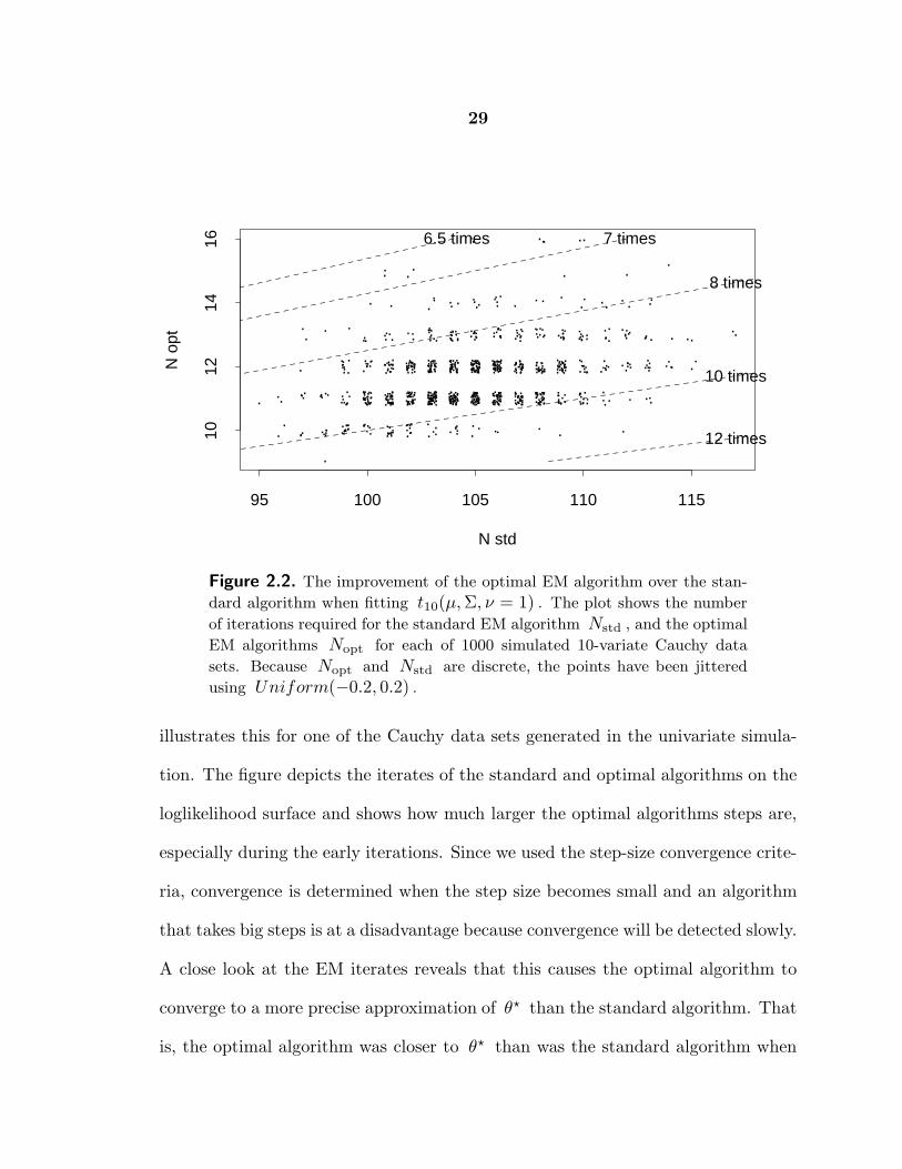
Figure 2.2. The improvement of the optimal EM algorithm over the stan-

dard algorithm when fitting t10(µ,Σ, ν = 1) . The plot shows the number

of iterations required for the standard EM algorithm Nstd , and the optimal

EM algorithms Nopt for each of 1000 simulated 10-variate Cauchy data

sets. Because Nopt and Nstd are discrete, the points have been jittered

using Uniform(−0.2, 0.2) .

illustrates this for one of the Cauchy data sets generated in the univariate simula-

tion. The figure depicts the iterates of the standard and optimal algorithms on the

loglikelihood surface and shows how much larger the optimal algorithms steps are,

especially during the early iterations. Since we used the step-size convergence crite-

ria, convergence is determined when the step size becomes small and an algorithm

that takes big steps is at a disadvantage because convergence will be detected slowly.

A close look at the EM iterates reveals that this causes the optimal algorithm to

converge to a more precise approximation of θ⋆ than the standard algorithm. That

is, the optimal algorithm was closer to θ⋆ than was the standard algorithm when

30

the convergence criterion was finally satisfied. The optimal algorithm converged

not only more quickly but also more precisely.

The difference between the two algorithms stems from the Q(θ|θ(t)) func-

tions which result from the two augmentation schemes. In particular, the opti-

mal algorithm results from less data augmentation and, hence, a flatter expected

augmented-data loglikelihood. This is depicted in Figure 2.4 for the same data set

that was used in Figure 2.3 and will be explored analytically in the following section.

2.4.2. Theoretical derivations

It now remains only to show that replacing (2.3.4) with (2.3.6) results in the algo-

rithm that is optimal in the class indexed by a . For a fixed a , the loglikelihood

for (µ,Σ) based on the augmented data Yaug(a) is

L(µ,Σ|Yaug(a)) =n

2[a(p+ ν) − 1] log |Σ| (2.4.1)

− |Σ|a∑i qi(a)

2

[ν + (yw − µ)⊤Σ−1(yw − µ) + tr(Σ−1Sw)

],

where

yw =

∑i qi(a)yi∑i qi(a)

and Sw =

∑i qi(a)(yi − yw)(yi − yw)⊤∑

i qi(a). (2.4.2)

It follows immediately that the MLE given Yaug(a) for µ is yw . In order to simplify

the derivation of the MLE of Σ , we will differentiate (2.4.1) with respect to the ele-

ments of Ψ = Σ−1 . The MLE of Σ is the solution of the resulting normal equation

31

θ(2) , optimal

θ(3) , standard

Figure 4. Comparing the optimal and standard iterative mappings. The figure shows the mappings induced

on L(θ|Yobs) by the standard algorithm ( + ) and the optimal algorithm (× ) for a one-dimensional Cauchy

data set fit with ν = 1 , starting from the same θ(0) (not shown). Notice how much larger the steps are

with the optimal algorithm.

32

Yobs

Yaug(aopt)

Yaug(astd)

Figure 5. Comparing the loglikelihoods. The plot shows L(θ|Yobs) , as well as E[L(θ|Yaug)|Yobs, θ⋆] for

both the standard and optimal augmentations (each adjusted by their maximum value for comparison).

Notice that the optimal augmentation results in a flatter loglikelihood that better approximates L(θ|Yobs) .

33

∂

∂ΨL(µ,Σ|Yaug(a)) =

− n

2[a(p+ ν) − 1] [2Σ − Diag(Σ)] (2.4.3)

− 1

2|Σ|a

∑

i

qi(a)[(yw − µ)(yw − µ)⊤ + 2Sw − Diag(Sw)]

+a

2

∑

i

qi(a)|Σ|a[2Σ − Diag(Σ)][ν + (yw − µ)⊤Σ−1(yw − µ) + tr(Σ−1Sw)],

which follows from∂

∂Ψtr(ΨSw) = 2Sw − Diag(Sw) , and

∂

∂ψij|Ψ| =

{2Ψij if i 6= jΨii if i = j

, (2.4.4)

where ψij is the ij th element of Ψ and Ψij is the ij th cofactor of Ψ (Mardia,

Kent, and Bibby, 1979, pp. 478-79), and Diag(A) denotes a diagonal matrix with

the same diagonal elements as A . Finally the chain rule along with (2.4.4) and the

standard matrix algebra result that Σ = (Ψij)/|Ψ| give us

∂

∂Ψ|Ψ|−a = a|Σ|a[2Σ − Diag(Σ)]

and

∂

∂Ψlog |Ψ| = 2Σ − Diag(Σ).

Evaluating (2.4.3) at the MLE of µ = yw and replacing [2Σ − Diag(Σ)] with Σ

and [2Sw − Diag(Sw)] with Sw , since we may solve (2.4.3) for each element of Σ

individually, we see that the MLE of Σ satisfies

n[a(p+ ν) − 1]

|Σ|a∑i qi(a)Σ + Sw = a[ν + tr(Σ−1Sw)]Σ. (2.4.5)

Solving (2.4.5) with arbitrary a is quite difficult, but there are two values of a

that make (2.4.5) trivial to solve. One is a = 0 , corresponding to the standard

34

augmentation scheme, which yields Σ = (∑

i qi/n)Sw and thus (2.3.4). The other

is aopt = 1/(ν + p) , with which the first term on the left side of (2.4.5) is zero,

and thus, the solution Σ must be proportional to Sw . It is then easy to verify

that the proportionality constant must be one, and therefore the MLE of Σ = Sw ,

which yields the corresponding M-step given by (2.3.6). It is arguably a miracle

that (2.4.5) can be solved analytically for the optimal a , but for (almost) no other

a .

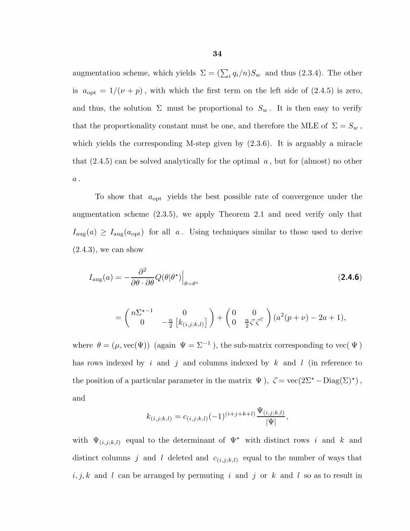
To show that aopt yields the best possible rate of convergence under the

augmentation scheme (2.3.5), we apply Theorem 2.1 and need verify only that

Iaug(a) ≥ Iaug(aopt) for all a . Using techniques similar to those used to derive

(2.4.3), we can show

Iaug(a) = − ∂2

∂θ · ∂θQ(θ|θ⋆)∣∣∣θ=θ⋆

(2.4.6)

=

(nΣ⋆−1 0

0 −n2

[k(i,j;k,l)

])

+

(0 00 n

2~ς ~ς⊤

)(a2(p+ ν) − 2a+ 1),

where θ = (µ, vec(Ψ)) (again Ψ = Σ−1 ), the sub-matrix corresponding to vec( Ψ )

has rows indexed by i and j and columns indexed by k and l (in reference to

the position of a particular parameter in the matrix Ψ ), ~ς = vec(2Σ⋆−Diag(Σ)⋆) ,

and

k(i,j;k,l) = c(i,j;k,l)(−1)(i+j+k+l) Ψ(i,j;k,l)

|Ψ| ,

with Ψ(i,j;k,l) equal to the determinant of Ψ⋆ with distinct rows i and k and

distinct columns j and l deleted and c(i,j;k,l) equal to the number of ways that

i, j, k and l can be arranged by permuting i and j or k and l so as to result in

35

the deletion of two distinct rows and two distinct columns. That is,

c(i,j;k,l) =

0 if three or four of i, j, k and l are equal1 if there are not three equal but i = j and k = l2 if no three are equal, i 6= j or k 6= l, but there are two equal4 if all four are distinct.

Given (2.4.6) it is easy to show

Iaug(a) − Iaug(aopt) = (ν + p)

(a− 1

ν + p

)2

C for any a,

where C is the positive semi-definite matrix

(0 00 n

2~ς ~ς⊤

)which does not depend

on a . Thus, the desired result that aopt = 1/(ν + p) minimizes the augmented-

information is clear. With the note that the E-step for the optimal EM only differs

from the standard E-step of (2.3.2) by a scale factor that is independent of i and,

thus, is irrelevant for (2.3.3) and (2.3.6), this completes our proof that replacing

(2.3.4) by (2.3.6) results in a uniformly faster EM algorithm regardless of ν , p or

Yobs .

2.5. Random Effects Models: New Fitting Algorithms

2.5.1. The standard EM algorithm

The random-effects (including variance-component) model is an increasingly com-

mon generalization of the standard linear model and is a routine, albeit sometimes

notoriously slow, application of the EM algorithm (e.g., Laird and Ware, 1982;

Laird et al., 1987; Liu and Rubin, 1995a). Here we assume

yi = X⊤i β + Z⊤

i bi + ei, bi ∼ Nq(0, T ), ei ∼ N(0, σ2), bi ⊥ ei, (2.5.1)

36

for i = 1, . . . , n , where Xi (p×1) and Zi (q×1) are known covariates; and β are

the (p×1) fixed effects; bi = (bi1, . . . , biq) are the (q×1) random effects. Although

there is no general closed-from solution for the maximum likelihood estimate θ⋆ ≡

(β⋆, σ2⋆, T ⋆) of θ ≡ (β, σ2, T ) given Yobs = (y1, . . . , yn) , the EM algorithm again

provides a simple and stable fitting algorithm. The standard data augmentation

(Dempster, Laird and Rubin, 1977; Laird and Ware, 1982; Laird et al., 1987) which

treats the bi as missing data (i.e., Yaug = {(yi, bi); i = 1, . . . , n} ) leads naturally

to the following algorithm. The E-step calculates the augmented-data sufficient

statistics:

b(t+1)i = E(bi|Yobs, θ

(t)) =T (t)Zi(yi −X⊤

i β(t))

[σ2](t) + Z⊤i T

(t)Zi, (2.5.2)

T(t+1)i = E(bib

⊤i |Yobs, θ

(t)) = b(t+1)i

[b(t+1)i

]⊤+ T (t) − T (t)ZiZ

⊤i T

(t)

[σ2](t) + Z⊤i T

(t)Zi. (2.5.3)

Since Q(θ|θ(t)) factors into two terms, one involving β and σ2 and the other

involving T , the M-step has a particularly simple form. First we update (β, σ2)

via the linear regression implied by (2.5.1),

β(t+1) =

(n∑

i=1

XiX⊤i

)−1( n∑

i=1

Xi(yi − Z⊤i b

(t+1)i )

)

(2.5.4)

σ2(t+1) =1

n

n∑

i=1

[(yi −X⊤

i β(t+1) − Z⊤

i b(t+1)i

)2

+ tr

(ZiZ

⊤i (T

(t+1)i − b

(t+1)i

[b(t+1)i

]⊤)

)].

Using the assumed marginal normality of bi , we then update T with the sums of

squares estimate

T (t+1) =1

n

n∑

i=1

T(t+1)i ,

37

thus completing a single iteration of the standard algorithm.

2.5.2. A new EM algorithm

In Section 2.3, we rescaled the missing data by a power of its standard deviation,

thereby introducing a working parameter into the data augmentation which results

in a remarkable EM implementation for the t -model. Inspired by this success,

we obviously wanted to try the same idea with the random-effects model given in

(2.5.1). Because in this setting the unobserved random variable b can be a vector,

the theoretical derivation is much more complicated. In principle, we can rescale

b by T−a/2 , where a is an arbitrary constant, and treat {bi(a) = T−a/2bi, i =

1, . . . , n} as the missing data. Since T can be any positive definite matrix and

it is difficult to handle an arbitrary power of a matrix, however, the resulting EM

algorithm is very difficult if not impossible to implement. This clearly violates our

requirement that the resulting algorithm not only needs to be fast but also needs

to be simple and stable.

There are two ways of getting around the difficulties that arise from dealing

with the matrix scale factor T . The first one is to deal only with a = 1 . (Recall

that the standard algorithm given above corresponds to a = 0 .) The second is to

diagonalize T so as to reduce the problem to q scalar problems. In this section, we

will derive the algorithm corresponding to a = 1 . At first, one might think that this

is rather restrictive and may not provide much computational gain. Surprisingly,

as we will illustrate in Section 2.6, the simple switch from a = 0 to a = 1 can

dramatically reduce the computation time. Nevertheless, in Section 2.5.3, we will

38

diagonalize T and create a more flexible class of data-augmentation schemes and,

thus, further improve computational efficiency.

To derive the new algorithm, we start by substituting bi = Sbi into (2.5.1),

where S is a symmetric matrix such that T = S2 . That is, we express the model

as

yi = X⊤i β + Z⊤

i Sbi + ei, bi ∼ Nq(0, I), ei ∼ N(0, σ2), bi ⊥ ei, (2.5.5)

for i = 1, . . . , n . By doing this, we convert the variance parameter T into the

regression parameter S . Note that such a conversion is not one-to-one since S is

not unique. However, this does not create a problem for our formulation because

we are only using S as an intermediate device for deriving algorithms, and the

parameter of interest, namely θ = (β, σ2, T ) , is uniquely determined and fitted

from the model.

Under model (2.5.5) we will treat Yaug = {(yi, bi), i = 1, . . . , n} as the aug-

mented data. Given this data, (2.5.5) can be fit via a simple linear regression with

missing values among the predictor variables. To see this more clearly, we re-express

the regression model in (2.5.5) as

y1y2...yn

=

X⊤1

X⊤2...

X⊤n

β +

Z⊤1

Z⊤2...Z⊤

n

S +

e1e2...en

, (2.5.6)

where Zi = VEC(Zib⊤i + biZ

⊤i ), S = VEC(S), with VEC(A) being a one-to-one

mapping from a q×q symmetric matrix A = (aij) to a q = q(q + 1)/2 dimensional

vector:

VEC(A) =

(a11√

2, a12, . . . , a1q,

a22√2, a23, . . . , a2q, . . . ,

aq−1,q−1√2

, aq−1,q,aq,q√

2

).

39

Here Zi, i = 1, . . . , n are unobserved, but follow Nq(0,Var(Zi)), with Var(Zi)

completely known because bi ∼ Nq(0, I) .

To implement the EM algorithm to fit (2.5.6), with Z ≡ [Z1, Z2, . . . , Zn]⊤

as missing data, we first notice that the augmented-data loglikelihood is linear in Z

and B ≡ Z⊤Z =n∑

i=1

ZiZ⊤i . Thus, at the (t+ 1) st iteration, the E-step computes

Z(t+1)i = E

[Zi|Yobs, θ

(t)]

= VEC(ZiE

[b⊤i |Yobs, θ

(t)]

+ E

[bi|Yobs, θ

(t)]Z⊤

i

)(2.5.7)

and

B(t+1)i ≡ E

[ZiZ

⊤i |Yobs, θ

(t)], (2.5.8)

for i = 1, . . . , n . The computation of (2.5.7) is straightforward because

b(t+1)i ≡ E

[bi|Yobs, θ

(t)]

=[S(t)

]−1

b(t+1)i

(see (2.5.2)) =S(t)Zi

(yi −X⊤

i β(t))

[σ2](t) +[S(t)Zi

]⊤ [S(t)Zi

] , (2.5.9)

where S(t) = VEC−1(S(t)) . The computation of (2.5.8) is a bit more involved,

because B(t+1)i is not a function of the matrix

T(t+1)i = E

[bib

⊤i |Yobs, θ

(t)]

(2.5.10)

(see (2.5.3)) = b(t+1)i

[b(t+1)i

]⊤+ Iq −

S(t)Zi

[S(t)Zi

]⊤

[σ2](t) +[S(t)Zi

]⊤ [S(t)Zi

] ,

but is rather a function of the elements of T(t+1)i , and some “bookkeeping” details

are required to express (2.5.8) as a function of the elements of T(t+1)i . In particular,

from the definition of the VEC operator, B(t+1)i is a function of

E

[(zij bik + zik bij)

2

∣∣∣∣Yobs, θ(t)

]= z2

ij

[T

(t)i

]kk

+ 2zijzik

[T

(t)i

]jk

+ z2ik

[T

(t)i

]jj,

40

where Zi = (zi1, . . . , ziq) , bi = (bi1, . . . , biq) , and[T

(t)i

]jk

is the jk th element of

T(t)i .

Once Z(t+1)i and B

(t+1)i are calculated for i = 1, . . . , n , the M-step finds

the maximizer of Q(θ|θ(t)) as

β(t+1)

S(t+1)

=

n∑

i=1

XiX⊤i

n∑

i=1

Xi

[Z

(t+1)i

]⊤

n∑

i=1

Z(t+1)i X⊤

i

n∑

i=1

B(t+1)i

−1

n∑

i=1

Xiyi

n∑

i=1

Z(t+1)i yi

(2.5.11)

and

[σ2](t+1)

=1

n

n∑

i=1

[(yi −X⊤

i β(t+1) −

[Z

(t+1)i

]⊤S(t+1)

)2

+ tr

(S(t+1)

[S(t+1)

]⊤(B

(t+1)i − Z

(t+1)i

[Z

(t+1)i

]⊤)

)]. (2.5.12)

Computationally, a way to avoid inverting the (p+ q) × (p+ q) matrix in (2.5.11)

is to use the SWEEP operator to perform the regression; for details see Little and

Rubin (1987, pp. 153-57). Upon convergence, we will compute T ⋆ = [S⋆]2, which

is always positive definite even though S⋆ may not be. Furthermore, as we noted

earlier, although S⋆ is not unique, T ⋆ is (given the regularity conditions that

guarantee the uniqueness of the mode of L(θ|Yobs) ).

2.5.3. Implementation of EM after diagonalization

We now describe a second approach, namely we will diagonalize (i.e., or-

thagonalize) T before we implement the EM algorithm. Let T = ∆U∆⊤ , where

∆ is a lower triangular (q × q) matrix with ones on the diagonal, and U is a

diagonal matrix. It is well-known that such a decomposition exists and is unique

41

(e.g., Horn and Johnson, 1985, p.162). Let ci = ∆−1bi , then ci ∼ Nq(0, U) .

Since U ≡ (u21, . . . , u

2q) is diagonal, we have the flexibility to rescale each element

of ci = (ci1, . . . , ciq)⊤ by a power of its own standard deviation. Specifically, for

any vector a = (a1, . . . , aq)⊤ ∈ R

q , we can define

ci(a) =

(ci1ua1

1

,ci2ua2

2

, . . . ,ciq

uaqq

)⊤

,

and treat Yaug(a) = {(yi, ci(a)), i = 1, . . . , n} as the augmented data. For a =

(1, 1, . . . , 1) , ci(a) = U12 ci = ∆U

12 bi . From the representation T = ∆U∆⊤ , it is

clear that this data augmentation stems from using the lower diagonal square root

matrix in place of the symmetric square root which was used in the previous section.

The re-expression of model (2.5.1) corresponding to this data augmentation is

yi = X⊤i β +

q∑

j=1

q∑

k=j

cij(a)zikδkjuaj

j + ei, (2.5.13)

where ∆ = (δkj) and ci(a) ≡ (ci1(a), . . . , ciq(a))⊤ . Although we can in principle

implement the EM algorithm for any a ∈ Rq which will result in a fast algorithm, we

will focus on a ∈ {0, 1}q . That is, ai can only take on values 0 or 1 in order to keep

the resulting algorithms simple to implement which is one of the main objectives of

our search. Within this class of data-augmentation schemes, given Yaug(a) , (2.5.13)

is a linear regression with p+q(q − 1)

2+

q∑

j=1

aj regression coefficients when we

view {δkjuj , k ≥ j, for aj = 1} ∪ {δkj ; k > j, for aj = 0} as theq(q − 1)

2+

q∑

j=1

aj

regression coefficients besides β . The M-step thus has two parts. First, we update

(β, σ2,∆, {uj, for aj = 1}) via the linear regression (2.5.13), performed in the same

way as described in Section 2.5.2, by treating {cij(a)zik, k > j}∪{cij(a)zij, for aj =

42

1} as the missing covariates. For example, for a = (1, 1, . . . , 1) , we can rewrite

(2.5.13) as

yi = X⊤i β + X⊤

i β + ei,

where Xi is a vector with components cij(a)zik for j = 1, . . . , q , k ≥ j and β

is a vector with corresponding components δkjuj . In this case, the parameters can

be updated by

β(t+1)

β(t+1)

=

n∑

i=1

XiX⊤i

n∑

i=1

Xi

[X

(t+1)i

]⊤

n∑

i=1

X(t+1)i X⊤

i

n∑

i=1

B(t+1)i

−1

n∑

i=1

Xiyi

n∑

i=1

X(t+1)i yi

(2.5.14)

and

[σ2](t+1)

=1

n

n∑

i=1

[(yi −X⊤

i β(t+1) −

[X

(t+1)i

]⊤β(t+1)

)2

+ tr

(β(t+1)

[β(t+1)

]⊤(B

(t+1)i − X

(t+1)i

[X

(t+1)i

]⊤)

)], (2.5.15)

where X(t+1)i = E

[Xi|Yobs, θ

(t)]

and B(t+1)i = E

[XiX

⊤i |Yobs, θ

(t)]

. Second, (for

any a ∈ {0, 1}q ) we update {uj, for aj = 0} by using cij(a) ∼ N(0, u2j) when

aj = 0 and thus

[u(t+1)j ]2 =

1

n

n∑

i=1

E

[c2ij(a)|Yobs, θ

(t)], for j such that aj = 0. (2.5.16)

The E-step is also quite similar to that described in Section 2.5.1. First we calculate

(corresponding to (2.5.9)–(2.5.11) or (2.5.2)–(2.5.3))

c(t+1)i (a) = E

[ci(a)|Yobs, θ

(t)]

=U (t)(2 − a)

[∆(t)

]⊤ (yi −X⊤

i β(t))

[σ2](t) + Z⊤i ∆(t)U (t)[∆(t)]⊤Zi

(2.5.17)

and

43

U(t+1)i (a) = E

[ci(a)c

⊤i (a)|Yobs, θ

(t)]

= c(t+1)i (a)

[c(t+1)i (a)

]⊤+ U (t)(2(1 − a))

−U (t)(2 − a)∆(t)Zi

[U (t)(2 − a)∆(t)Zi

]⊤

[σ2](t) + Z⊤i ∆(t)U (t)

[∆(t)

]Zi

, (2.5.18)

where U(d) ≡ Diag

{[u

(t)1

]d1

, . . . ,[u(t)

q

]dq

}for d = (d1, . . . , dq) . We then use the

elements of c(t+1)i (a) and U

(t+1)i (a) , i = 1, . . . , n to calculate the augmented-data

sufficient statistics. In particular, E[c2ij(a)|Yobs, θ

(t)]

needed for (2.5.16) is simply

the j th diagonal term of U(t+1)i (a) , and the augmented-data sufficient statistics

needed for the regression (i.e., the input for the SWEEP operator or the terms needed

in (2.5.14) and (2.5.15)) are

E

[cij(a)zik

∣∣Yobs, θ(t)]

= zik c(t+1)ij (a),

for j = 1, . . . , q and k ≥ j and

E

[cij(a)zikcil(a)zim

∣∣Yobs, θ(t)]

= zikzim

[U

(t+1)i (a)

]jl,

for j = 1, . . . , q , k ≥ j , l = 1, . . . , q and m ≥ l , where c(t+1)ij (a) is the j th com-

ponent of the vector c(t+1)i (a) and

[U

(t+1)i (a)

]jl

is the jl th element of U(t+1)i (a) .

Once the algorithm has converged, it is easy to compute the original parame-

ter T = Var(b) = Var(∆c) = ∆U∆⊤ . It should be noted that fitting the regression

model (2.5.13) can result in negative values for the {u⋆j , j = 1, . . . , q} . This should

not be cause for alarm, however, since ∆⋆U⋆∆∗⊤ will remain positive definite and

unique as long as T ⋆ is. In fact, since ∆ and U are unique for each T , there are

44

exactly 2q modes of L(β, σ2, U,∆|Yobs) (corresponding to the 2q diagonal roots

of U ) for every mode of L(β, σ2, T |Yobs) .

We now have 2q + 2 algorithms that are straightforward to implement and

which will generally converge to a local maximum of L(θ|Yobs) . In order to evaluate

the relative computational merits of the algorithms, we will first present an empirical

study and then analyze the algorithms in terms of their matrix and global rates of

convergence.

2.6. Random Effects Models: Empirical Results

and Theory

2.6.1. Simulation Studies

Two sets of empirical studies were conducted, each with data generated from

the model

yi = xi1β1 + xi2β2 + zi1bi1 + zi2bi2 + ei, (2.6.1)

where xi1 = 1, xi2 = i ,

(b1b2

)∼ N2

(0,

(4 00 9

)), and ei ∼ N(0, σ2) , with bi

and ei independent. In the first set of studies, (2.6.1) was treated as a variance-

component model (with covariates) and (zi1, zi2) took the four values in {0, 1}2 in

equal proportion. In the second set of simulations, (2.6.1) was treated as a random-

effects model and the zij were generated independently from a standard normal

distribution at each replication.

As we shall see, the relative efficiency of the algorithms depends on the rela-

45

tive sizes of the random effects and the residual variance. The variance-component

study was therefore repeated with σ2 = 1, 4, 9 and 36 . For each of these val-

ues, we generated 100 observations from (2.6.1). The starting values β(0) and

[σ2](0)

were obtained by fitting (2.6.1), ignoring the variance components, and

T (0) was set to

(1 0.1

0.1 1

). We ran the standard algorithm along with EM (0,0)

and EM (1,1) , that is the new algorithm with Yaug((0, 0)) and Yaug((1, 1)) respec-

tively (i.e., with a = (0, 0) and a = (1, 1) ), and recorded Nstd , N(0,0) , and N(1,1)

– the number of iterations required by each algorithm before the convergence crite-

rion L(θ(t)|Yobs)−L(θ(t−1)|Yobs) < 10−7 was reached. The simulation was repeated

200 times and the results appear in Figure 2.5.

The scatter plots in the first column of the figure compares N(0,0) with Nstd .

When σ2 = 1 , using Yaug((0, 0)) requires slightly more iteration than the standard

algorithm, but the two algorithms seem quite comparable. The second column of

Figure 2.5 compares N(1,1) with Nstd and highlights the great computational

savings EM (1,1) offers over the standard algorithm, especially when σ2 is large

relative to T . In particular, with σ2 = 36 (about 5.5 times the average random

effect, 1n

∑i Z

⊤i TZi ), it was not unusual for the standard algorithm to require 100

times more iterations to converge, and sometimes it took 600 times more. Since all

of the algorithms require roughly the same computational time per iteration, this

translates into real computational savings. For example, an older Sun Workstation

might compute about 30 iterations of any one of the algorithms per second, in which

case the data cloud to the right of the scatter plot corresponding to EM (1,1) with

σ2 = 36 represents 12.5 minutes being cut to between 1 and 10 seconds.

46

EM (0,0) EM (1,1)

4 6 8 10

46

810

log(Nstd)

log(

N(0

,0))

equal10x100x500x

10x

100x

500x

4 6 8 10

46

810

log(Nstd)

log(

N(0

,0))

equal10x100x500x

10x

100x

500x

4 6 8 10

46

810

log(Nstd)

log(

N(0

,0))

equal10x100x500x

10x

100x

500x

4 6 8 10

46

810

log(Nstd)

log(

N(0

,0))

equal10x100x500x

10x

100x

500x

4 6 8 10

46

810

log(Nstd)

log(

N(0

,0))

equal10x100x500x

10x

100x

500x

4 6 8 10

46

810

log(Nstd)

log(

N(0

,0))

equal10x100x500x

10x

100x

500x

4 6 8 10

46

810

log(Nstd)

log(

N(0

,0))

equal10x100x500x

10x

100x

500x

4 6 8 10

46

810

log(Nstd)

log(

N(0

,0))

equal10x100x500x

10x

100x

500x

σ2

=1

σ2

=4

σ2

=9

σ2

=36

Figure 2.5. Comparing the log number of iterations required by EM (0,0)

and EM (1,1) for convergence with that of the standard algorithm. In the

plot “100x” means “100 times”, etc. On a computer that runs 30 iterations

per second, the tick marks 4, 6, 8, and 10 on the X and Y axes correspond

to 1.8 seconds, 13.4 seconds, 1.7 minutes, and 12.2 minutes.

47

Even when σ2 = 1 (less than one sixth the average random effect) EM (1,1)

tended to be slightly more efficient than the standard algorithm. When the residual

variance is small, however, using EM (1,1) tends to offer more modest gains over the

standard algorithm. In order to examine how the algorithms compare when the

residual variance is very small, the simulation was repeated with σ2 = 1/9 (about

one sixtieth of the average random effect). The results appear in Figure 2.6 and in-

dicate that the standard algorithm tends to be about 2.7 times faster than EM (1,1) .

Note, however, that N(1,1) is centered around e7 ≈ 1100 iterations (37 seconds

at 30 iterations per second) compared with the e10 ≈ 22000 (12.2 minutes) when

the standard algorithm was slow (see Figure 2.5). In this simulation, the standard

algorithm seems to be more efficient only when both algorithms are relatively fast.

Whereas EM (1,1) is more efficient when the standard algorithm is very slow and

improvement is badly needed (see Figure 2.7). Thus, unless the residual variance

is very small relative to the random effects, EM (1,1) seems to be the algorithm to

choose.

The second set of simulations was identical to the first except that in order

to look at the more general random-effects problem, the zij were independently

generated from a standard normal distribution. The simulation was repeated for

σ2 = 0.25, 1, 4, 9, 16, 25, 36, 49, 64, and 81. Again, we want to compare the

efficiency of the standard EM algorithm with EM (1,1) as a function of the relative

sizes of the residual variance and the random effects. In the previous simulation T

and {Zi, i = 1, . . . , n} were fixed, and it sufficed to consider efficiency as a function

of σ2 . Since {Zi, i = 1, . . . , n} changes at each replication in the current simula-

48

log(Nstd)

log(

N(1

,1))

4 6 8 10

46

810

equal10 times100 times500 times

10 times

100 times

500 times

Figure 2.6. Performance of EM (1,1) when the residual variance is very

small. Here σ2 = 1/9 and the average random effect is 6.5. Note that

the median number of iterations required by EM (1,1) is e7 = 1142 (38

seconds) which is less efficient than the standard algorithms e5.26 = 194iterations (6.4 seconds).

tion, we look at the log of the number of iterations required for convergence as a

function of log(σ2⋆/ 1n

∑i Z

⊤i T

⋆Zi) . (This expression is evaluated at the MLE since

the matrix rate of convergence, I − IobsI−1aug is evaluated at the MLE.) Figure 2.8

displays a sequence of scatter plots. The first displays the efficiency of the standard

algorithm, which does well only when the residual variance is somewhat smaller

than the average random effect. The second scatter plot looks at EM (1,1) which

continues to do very well when the residual variance is large, but does not perform

as well when the residual variance is small. Note that when the residual variance

was small, both algorithms perform poorly in this simulation, as opposed to the

variance-component simulation in which both algorithms performed well. The final

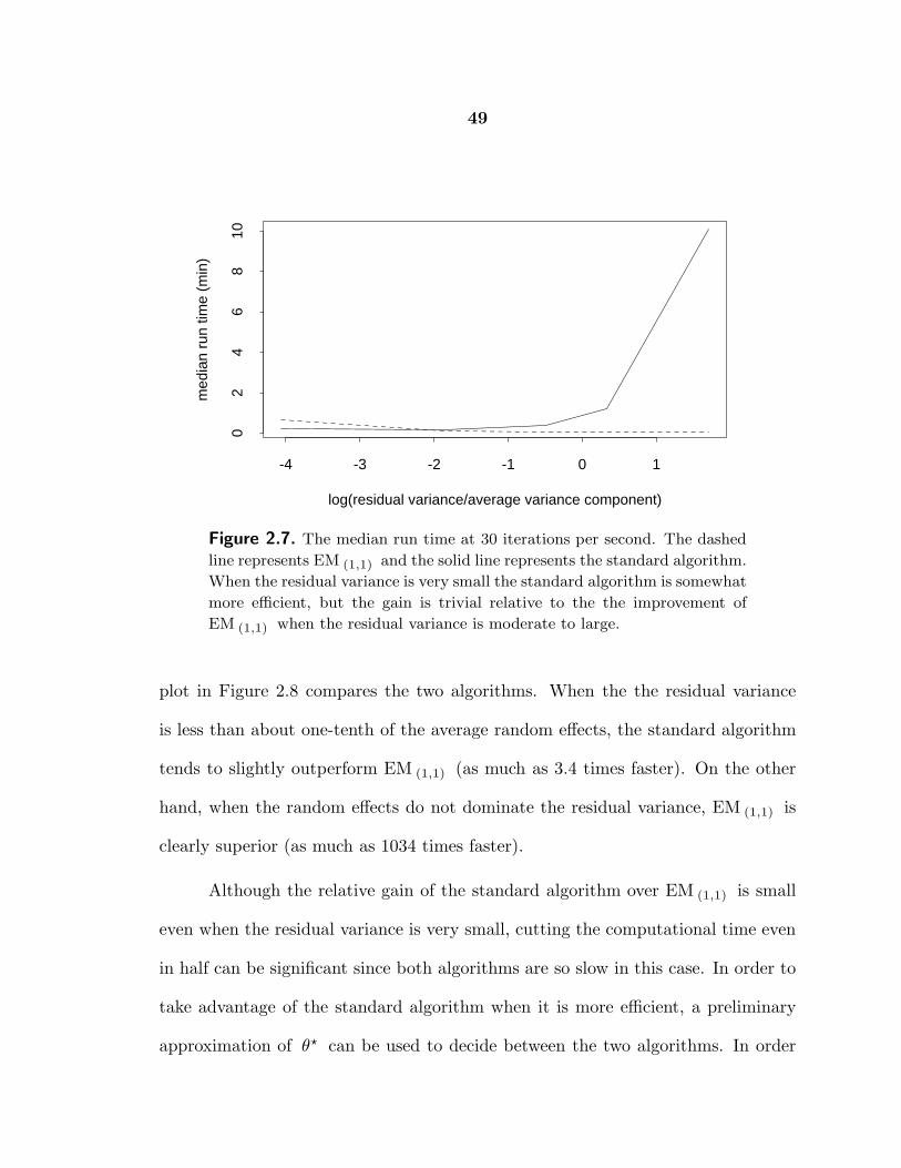
49

log(residual variance/average variance component)

med

ian

run

time

(min

)

-4 -3 -2 -1 0 1

02

46

810

Figure 2.7. The median run time at 30 iterations per second. The dashed

line represents EM (1,1) and the solid line represents the standard algorithm.

When the residual variance is very small the standard algorithm is somewhat

more efficient, but the gain is trivial relative to the the improvement of

EM (1,1) when the residual variance is moderate to large.

plot in Figure 2.8 compares the two algorithms. When the the residual variance

is less than about one-tenth of the average random effects, the standard algorithm

tends to slightly outperform EM (1,1) (as much as 3.4 times faster). On the other

hand, when the random effects do not dominate the residual variance, EM (1,1) is

clearly superior (as much as 1034 times faster).

Although the relative gain of the standard algorithm over EM (1,1) is small

even when the residual variance is very small, cutting the computational time even

in half can be significant since both algorithms are so slow in this case. In order to

take advantage of the standard algorithm when it is more efficient, a preliminary

approximation of θ⋆ can be used to decide between the two algorithms. In order

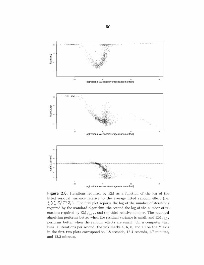
50

-10 0 10 20

46

810

log(residual variance/average random effect)

log(

Nst

d)

.

.

..

.

.

.

.

.

.

.

.

.

.

.

.

.

.

.

.

.

.

..

.

.

.

. .

.

..

.

...

.

..

.

.

.

..

..

.

.

.

.

.

..

..

.

.

.

.

.

.

.

...

.

.

.

.

.

..

. .

.

.

.

. .

.

.

.

.

.

.

.

. .

..

... .

..

.

..

.

.

.

.

.

. .

. .

.

.

..

.

.

.

. .

.

.

...

. .

.

..

.

..

.

.

.

..

.

.

.

.

...

.

.

..

.

. .

.

.

..

.

.

. .

.

.

.

.

..

.

...

. .

. .

.

..

..

.

.

..

.

.

.

..

.

. .

.

.

.

.

..

. .

.

.

.

.

.

.

.

.

.

..

..

.

.

. ..

..

.

.

.

.

..

.

..

.

.

.

.

..

.

.

.. .

. .

. .

.

.

.

...

.

.

.

. .

.

.

....

.

.

.

.

...

.

.

.

.

..

.

..

.

. ..

..

..

..

.

.

.. .

..

.

.

..

...

.

.

.

.

.

.

...

.

.

.

.

.

.

.

.

.

.

.

.

.

. .

..

.

.

.

.

.

.

.

. . ..

.

.

.

..

.

.

.

.

.

.

.

.

.

.

..

..

.

.

.

.

.

.

.

.

..

.

.

.

.

.

.

.

.

.

.

.

.

..

.. ...

..

.

.

.

.

.

...

..

.....

. ...

.

.

.

. ..

.

.

.

.

.

..

.. ...

.

.. .

.

..

. .

.

.

..

.

. .

.

...

.

.

..

..

.

..

.

. .

..

.

. ..

. .

..

.

.

.. ..

.

.

.

..

..

.

.

.

.

.

.

.

.

... .

.

.

.

..

.

.

..

..

.

..

.

.

.

. ..

.

..

.

..

.

..

.

.

.

.

.

.

..

.

..

.

.

..

..

.

.

.

.

.

.

.

.

.

..

. .

..

.

.

....

.

.

...

.

...

..

..

.

.

..

..

.

..

.

...

.

.

....

.

..

.. . . .

.

.

...

.

.

.

..

..

.

.

..

.

.....

.

.

.

.

..

.

.

.

.

..

.

..

..

..

..

.

..

.

.

..

.

.

.

.

.

.

.

...

.

..

...

.

. .

.

..

.

.

..

.

.

.

..

.

.

.

.

.

.

.

.

.

.

. . .

.

.

..

.

.

.

.

..

.

.

.

.

.

.

.

.

.

.

.

. .

.

.

.

.

.

.

.

.

.

. .

.

.

..

..

.

.

..

.

.

.

.

.

..

.

.. .

.

.

..

.

.. ..

..

.

.

.

. .

. .

.

.

.

.

.

..

..

.

.

.

..

.

.

..

.

.

.

.

..

.

.

..

.

.

.

.

.

.

.

.

.

.

.

.

.

..

.

..

.

.

.

.

.

..

.

.

. .

.

.

.

..

.

.

.

.

.

.. .

.

..

.

.

.

. .

.

.

.

.

.

..

.

. .. .

..

.

.

.

.

.

.

. ..

.

.

.

..

.

.

.

..

.

.

.. ..

.

..

.

.

..

.

.

.

.

.

.

. .

..

.

.

. .

.

.

.

.

..

...

.

.

. .

..

.

.

.

..

.

. .

.

.

. . ..

..

..

..

. .

.

...

..

.

.

.

.

.

..

.

.. ..

.

.

.

.

.

.

.

.

.

.

.

.

.

.

..

...

.

.

.. ...

..

.

.

.

.

.

.

.

.

.

.

..

.

.

.

..

.

.

.

.

.

...

.

.

.

.

.

.

.

.

.

.

..

.

.

..

.

.

.

. .

.

..

.

.

.

..

.

.

.

.

.

...

.

.. .. .

.

.

.

.

.

.

..

.

.

..

.

.

. .

.

.

.

.

.

.

.

.

.

.

.

.

.

.

.

.

.

..

.

.

. ..

.

..

.

. .. .

.

.

..

..

.

.

.

..

.

.

.

.

..

.

..

.

...

. .

.

.

..

.

.

.

.

.

...

.

.

.

..

..

.

.

.

.

.

..

.

.

.

.

.

.

.

.

.

.

.

.

.

.

.. .

.

..

. .

.

.

.

.

. .

.

..

..

.

.

..

..

.

.

..

.

.

.

.

..

.

.

.

. .

..

.

..

.

..

.

.

...

.

.

..

.

.

..

.

. . ...

.

..

.

.

..

. ..... .

.

.

..

.

. .

.

. .

.

.

..

.

.

.

.

.

..

.

.

.

.

.

... . .

.

... .

.

.

.

. .

. .

. .

.

.. .. . ..

.

...

. ...

.

.

....

..

..

.

.

.

.

.

.

.

.

.

.

.

.

.

.

.

. ..

..

...

.

..

.

.

.

.

..

.

.... .. .

.

.

. . .. ... .

. ..

.

..

.. ..

.

.

..

.

...

.

.

.

.

.

.

.

.

.

.

.

.

..

.

.

.

.

..

..

.

.

. ... .

.

.

. .

. .

..

.. .

.

. .. ..

.

.

.

.

. .

.

.

..

.

.

.

.

.

.. .

.

... ...

.

.

.

.

.

...

.

.

..

..

.

.

.

.

.

.. ..

.

...

.

. ... .

.

.

.

.

.

.

.

.. ...

.

.

.... .

.

... .

.

.

. .

.... .

..

.

. ...

.

. ....

.

..

.

.

.

.

..

.

..

..

.... .

.

.

.. ....

.

.

..

.

.

.

.

.

..

.

. .

.

.

.

.. . .

.

..

.

... . .

.

.

.

..

.

....

.

. . .

.

.

.

.

.

. ..

...

.

.

...

.

.

.

.

.

.

.

..

.. .

.

..

.

.

....

..

...

.

.

.

.

. .

.... .

.

.

.. ..

.

.

.

.. .

.

.

.

..

.

.

..

. . ..

.

..

.. .

.

.. .

.

.. ..

.

.

.

.

..

.

..

.

.

...

.

.

.

..

.

.

.

..

..

.

.

.

. .

.

..

.

.

.

...

.

.

.

.. ... .

.

.

. .. .... .

.

..

.

. .. . .

.

.

..

.

. ..

.

..

. ...

. .

..

.

..

.

. ..

..

.

...

.

. .

.

.. ..

.

.

.

..

..

..

.

..

.. .

.

.

.

.. .. . ..

.

. . .. ... . .

.

.

.

. .

.

. .

.

..

.

. .

.

..

..

.

. ..

.... . .. .. .

.

..

.

..

..

. ..

.

.

.

.... .. ..

..

.. ..

.

.

.

.

. ... . .

..

.... .. .

.

.

.

..

. ... ...

.

. ..

.

. .. .. . ...

.

. .

.

.. ..

. ...

.

.. .. . .

.

.

.

.

. ....

.

. . . ..

.

.. ..

.

.. .

.

.. . ..

.

. .

-10 0 10 20

46

810

log(residual variance/average random effect)

log(

N(1

,1))

.

.

..

.

..

.

.

.

.

.

.

.

.

.

.

.

.

.

.

.

..

.

.

.

..

.

..

.

..

.

.

.

.

.

.

.

..

..

.

.

.

.

.

.

.

..

.

.

.

.

.

.

.

..

.

.

.

.

.

.

..

. .

.

.

.

. .

.

. .

.

.

.

.

. .

.

..

.. .

..

.

..

.

.

.

.

.

. .

..

.

.

..

.

.

.

. .

.

.

..

.

. .

.

..

.

...

.

.

..

.

.

.

.

...

..

.

.

.

.

.

.

.

..

.

.

. .

.

.

.

...

.

...

.

.

.

.

.

.

.

..

.

.

..

.

.

.

..

.

. .

.

.

.

.

.

.

. .

.

.

.

.

.

.

.

.

.

..

..

.

.

..

...

.

.

.

.

..

.

.. .

.

.

.. .

.

.

.. .

. .

..

.

.

..

. .

.

.

.

..

.

.

. .

...

.

.

.

.

.

.

.

.

.

..

.

...

.

. ...

.

..

.. .

.

. ....

.

.

..

....

.

.

. .

.

..

.

.

.

.

.

.

.

.

..

.

..

.

.

..

.

.

.

.

.

.

.

.

. . ...

.

..

.

.

.

.

.

.

.

.

.

.

.

.

.

. ...

.

.

.

.

.

.

..

.

.

.

.

.

..

.

.

.

.

.

.

.

.. ..

..

.

.

.

.

.

.

...

. .

...

..

.

..

. ..

..

.. .

.

.

.

.

..

.

. ... ..

.

.

.

.

.

.

..

.

..

..

...

... ... .

. ...

.

....

..

..

..

.

.

.

...

..

.

.

.

.

..

.

.

... .

.

.....

..

.

.

.

..

.

..

..

.

. .

..

.

.....

..

.

.

.

. .. .

.

. .

..

..

. .

. ..

..

.

.

..

..

..

.

... .

...

.

.

..

.

..

.

...

..

...

. . ..

....

..

.

. .

..

..

.

..

.

..

.

... .

..

....

.

.

..

..

..

..

.

.

.

.. .

..

.

...

. .

.

.

.

.

.....

.

.

...

.

.

. .

.

...

.

.

. .

.

. ..

..

..

...

.

.. . .

..

.

.

. . .

.

...

.

.

.

...

.

..

.

.

. .

. ...

..

..

.

.

.

. .

.

.

.

.

.

.

.

.

. ..

.

.

.

.

.

.. ..

.

.

.

..

... .. .

. .

.

.

..

..

..

..

.

..

... .

.

.

. ..

.

.

.

.

.

..

.

.

.

. .

..

..

..

. ....

.

. .. .

.

....

. .. .

.

.

.

. .

.

.

..

.

.

.

..

.

.

..

.

.

.. .. .

.

.

..

.

.

.

.

.

.

.

. .

...

.

..

.

..

..

.

....

.

.

.

...

.

.

.

.

..

.

..

...

.

.

.

.

.

..

..

..

.

.

.

..

....

.

..

. .

. . .. . .

. . ..

.

.

..

...

..

.

...

.

.

.

...

.

.

.

...

. .

...

.

.

..

. ..

.

.

.

.

.

.

..

.

.

..

. .

.

.

.

.

.. ... .

..

.

.

..

.

.

..

..

.

. .

..

.

.

..

....

.

. ... .

.

.

.

..

..

.

.

.

.

..

.

..

.

.

.

.

..

.

.

...

.

.

.

.

.

..

. ..

.

.

.

..

..

.

..

.

.

..

..

.

..

.

..

. ..

..

.. ..

...

..

.

.

.

..

.

.

.

.

.

.

..

.

..

.

. .. ..

.

.

.

..

.

.

.

..

.

... .

.

.. .

..

.

.. ...

.

.

..

.

...

.

.

.

.

..

.

.

.

.

. .

.

.

.

..

. ... ..

.

.

.

.

.

.

.

.

.

..

.

.

.

..

..

..

...

.

.

. ..

..

.

.

.

. .

.

..

.

..

.

..

..

..

.

.

.

.

. ..

.

..

..

.

.

.

.

.

.

.

..

..

.

..

..

.

..

..

..

....

..

..

..

.

.

.

.

..

.

.. ..

.

.

.

.

.

.

.

.

.

.. .

..

...

..

..

..

.

. .

..

.

.

. .

.

..

.

.. .

. ...

..

.

.

. .

.

...

. ..

.

.

.

..

..

.

.

. .

.

.

.

.

..

..

.

.

.

..

..

. ..

..

..

...

.

.

..

. ..

.

..

.

.

..

. .

.. .

.

..

.

.

.. .

.

... .. .

.

..

.

.

.

.

.

.

. .

. .

.

.

.

.

.

..

.

.

.

...

.

.. ..

..

..

.

.

.

.

.. ..

.

.

.

.

.

.

.

.

..

.

.

.

. .

.

.

..

.

. ..

. .

.

.

..

.

..

.

.

.

.

.

.

.

..

.

.

.

.

..

.

.

.

.

..

. ..

.

.

.

.

.

.

.

.

.

.

..

.

..

..

..

.

. .

.

..

.

.

.

.

..

.

..

.

..

.

... .

.

..

.

.

.

..

.

...

..

.

.

..

. .

.

.

...

.

.

.

.

.

.

.

.

.

.

. ..

. .

.

.

.

.

.

.

.

.

.

.

.

.

.

.

.

.

.

..

.

...

.

.

.

.

..

.

..

.

.

..

.

...

.

.

..

.

.

.

.

.... .

.

.

.

.

... .

.

.

.

.

.

..

..

.

.

..

.

..

.

. .

.

.

.

.

.

..

.

.

. ..

.

.

.

.

.

...

..

.

.

.

..

.

.

..

.

.

...

.

..

.

.

..

.

.

.

.

...

..

..

.

.

..

.

.

.. .

.

.

.

..

.

..

..

..

.

..

..

.

.

.

.

.

..

.

.

..

.

...

.

.

..

..

.

.

.

.

.

. .

.

.

.

..

..

.

..

.

.

..

..

.

.

.. .

.

...

.

.

. .

.

.

. .

. .

.

.

.

...

..

..

. .

.

.

..

.

.

.

.

.

.

.

.

..

.

.

.

.

.

..

..

..

..

.

.

.

.

...

.

.. . .

.

.

.

...

.

.. .

..

.

.

.

.

.

. .

.

.

.

.

.

.

.

.

.

.

..

.

...

.

.

..

..

.

..

.

.

.

.

...

.

.

.

.

. .

.

.

.

..

.

. .

.

..

.

..

.

.

.

.

.

...

.

.

..

....

.

.

. .

.. .

..

.

.

.

..

...

.

.

..

.

.

.

.

.

.

..

.

.

...

.

. .

.

.

.

.

.

.

..

..

.

.

.

.

.....

.

.

.

..

.

.

.

.

.

..

.

. .

..

.

.

.

..

.

.

.

.

-10 0 10 20

-6-4

-20

24

6

log(residual variance/average random effect)

log(

N(1

,1)/

Nst

d)

. .... .. .. .. .... .. .. .. ... ...

... . .. .. ..

....

.. ... .

... ... ... . .. .. ... . ... .. . .. . .... .

..

.

. .. .. . ..

.

.. . ......

. .. .. . . .. ... .. .. . . .... . .... . ..

.. ... .. ..... .. ... .

.

.... ... . .. . .......

...

.

..

.

.. .. .. .. .. . . . .. ..

.. .. . ..

..

.. .. . .. .... .

..... .. .

... .. ...

.. ... .. .. . .

... ..

. ...

. . .. .. ..... ...

.

. .

.

.

.

..

.

..

. . .. . .. ..

. ... . .

.... .. ...... .

.. ...

.. . .

.

.. .. . ..

. ..

..

. .. ... .. . .....

... . .. .

.. ..

... . ..

.

. .. ... ... .... .

.. .. ..

.... .. ..

.. .. .. .. .. . ..... .

...

.

..

...

.

. .

.

.

...

. ...

..

..

.

.

..

.

.

. ..

.

...

...

.

.

...

.

.

. .

.

..

.....

..

.

... .

...

.

.

.

... ..

.

...

.

.

.

....

..

.

.

. ..

..

.

..

. ..

.

.. . ..

.. .

.. .

.

...

.

..

.

.

. .. . ..

.

.

..

.

..

.

.

.

.. ..

..

. ... .

. ..

.... ... . .....

..

.

..

.

..

.

..

.

...

.

...

.

.

.

.

.

..

..

..

.

...

.

..

..

..

.

.

..

..

. ... .

..

.

. ...

.

.

..

.

..

.

.

..

..

.

..

.

...

.

.

.

.

.

.

.

..

. ..

.

..

.

.

. .

.

.. .

.

..

.

.

...

.

.

.

..

..

.

.

..

. .

..

..

.

.

.

.

.

.

.

.

...

.

.

.

.

.

.

. .. ...

.

.

.

.

.

.

.

.

.

..

..

.

.. .

.

. .

.

..

.

.

....

.

.. ... .

...

.

.

.

..

..

..

.

.

.

. .

..

.

.

..

.

.

... ..

.

.

..

.

.

..

.

.

.

.

.

.

.

..

.

.

.

.. .

.

..

.

.

.

.

.

..

.

.. . .

.

.

..

.

.

.

.

.

.. . .

..

.

..

.

.

.. .

.

.

...

..

.

.

..

.

..

.

.

.

...

.

.

.

..

.

.

..

..... .

.

.

..

.

.. .

.

..

.

... .

. ...

. .

.

.

.

.

.

.

..

. .

.

. .

.

.

..

.

..

.

..

..

.. .

.

..

.

.

..

. .

.

.

..

. .

...

.

.

..

.

.

.

.

..

.

.

.

.

.

.

.

.

.

.

.

.

.

.

.

..

...

..

..

..

. ..

.

.

.

.

.

.

.

..

.

.

.

.

..

.

.

.

.

.

.

.

.

. ..

.

..

.

.

.

.

..

.

.

.

.

.

..

. ..

..

.

.

.

..

..

.

.

.

..

..

.. .

.

.

..

.

.

.

.

..

.

.

..

.

.

..

.

.

.

.

.

.

.

.

.

..

.

.

.

.

.

.

..

.

.

.

.

.

.

.

.

.

.

..

.

.

.

..

.

.

.

.

.

..

.

.

.

.

..

..

.

....

.

.

.

.

. .

.

..

.

.

.

.

.

..

..

.

..

..

.

. .

..

.

.

..

.

.

.

.

.

..

.

.

.

.. .

.

.

.

. .

.

.

.

.

..

..

.

...

.

..

..

.

.

..

.

..

.

. .

.

..

. .

...

..

..

.

.

.

..

.

.

.

...

.

...

..

...

.

..

.

.

..

.

..

...

.

.

.

..

.

.

.

.

.

.

.

.

..

.

.

.

.

.

..

.

.

.

.

.

.

.

. .

.

.

..

. .

.

.

.

.

.

. .

. .

.

.

. .

..

. .

... .

. ..

.

..

..

..

. .

. .

.

... .

.

.

.

.

..

.

.

.

.

. ..

..

..

.

.

.

.

..

.

.

..

.

..

.

.

..

. .

.

. .

.

. ..

.

.

. ..

.

..

.. .

..

.

..

.

.

.

.

.

.

..

..

..

..

.

.

..

.

.

.

.

..

..

..

..

.

.

.

.

.

. .

..

.

.

.

.

.

.

...

.

..

.

.

.

.

.

.

.

..

.

.

.

..

.. .

.

.

.

.

.

..

..

.

..

.

.

.

.. .

.

..

...

.

.

.

.

.

.

...

.

.

...

.

.

.

..

.

.

..

.

.

...

..

.

...

.

.

.

..

.

... .

.

...

.

.

..

.

... .

..

...

.

.

. .

.

.

.

.

. .

.

.

.

.

.

... .

..

..

.

.

.

.

.. .

.

.

..

.

.

.

.

.

. .

...

..

.

.

.

..

.

..

..

.

.

.

.

..

.

.

..

.

..

.

.

..

.

.

..

.

.

...

.

.

.

.

.

.

.

.

.

.

.

.

..

.

. ..

. .

.

.

..

.

.. .

.. .

...

.

.

.

....

.

..

.. .

.

.

.

.

...

.

.

.

..

.

.

..

.

..

.

.

..

...

.

.

.

.

.

.

.

..

.

.

.

.

.. .. .

.

.

..

.

..

.

..

....

.

.

.. ...

.

.

.

.

..

.

...

.

.

.

.

. .

..

.

..

..

...

...

.

. .

.

..

. ..

..

..

.

. .

..

. .. .

.

.

..

..

.

..

.

. ..

..

.

.

.

.

.

.

..

.

. .

. ..

.

.

.

.

.

.

.

.

..

.

.

.

.

.

.

.

.

.. . .

..

.

....

.. .

.

..

.

.

.

.

. .

.

.

. .

..

..

...

.

..

....

..

...

..

.

.

.

.

. ..

..

.

..

.

.

..

..

.

. .

.

. .

.. .

.

.

.

.

.

. ..

.

.

.

.

.

. ...

.

. .

.

.

...

..

.. .. .

.

.

.

.

.

.

.

..

.

...

.

.

. .

. .

. . .

.

.

.

.

.

..

..

..

.

.

.

.

...

.

.

.

. .

.

.

.

.

.

. .

.

.

.

. ..

.

.

..

.

..

.

Figure 2.8. Iterations required by EM as a function of the log of the

fitted residual variance relative to the average fitted random effect (i.e.1n

∑i Z

⊤i T

⋆Zi ). The first plot reports the log of the number of iterations

required by the standard algorithm, the second the log of the number of it-

erations required by EM (1,1) , and the third relative number. The standard

algorithm performs better when the residual variance is small, and EM (1,1)

performs better when the random effects are small. On a computer that

runs 30 iterations per second, the tick marks 4, 6, 8, and 10 on the Y axis

in the first two plots correspond to 1.8 seconds, 13.4 seconds, 1.7 minutes,

and 12.2 minutes.

51

to investigate this, we repeated the random-effects simulation (with new random

seeds) with an adaptive algorithm, which first runs EM (1,1) for 20 iterations and

then switches to the standard algorithm if

4[σ2](20) ≤ 1

n

∑

i

Z⊤i T

(20)Zi. (2.6.2)

This criterion is based on the result of the following section that when T is assumed

diagonal in the fitted model, aj should be set to zero in the data-augmentation

scheme (2.5.13) only if 2σ2⋆ ≤τ2⋆j

n

n∑

i=1

z2ij , where τ2⋆

j is the MLE of the j th

diagonal term of T . If we add this expression over j = 1, . . . , q and adjust for

non-diagonal T , we obtain (2.6.2) with the 4 being replaced by 2q . As Figure 2.9

indicates, this algorithm almost always switched to the standard algorithm when

it was beneficial to do so. (Surprisingly, the switched algorithm was often slightly

faster than the pure standard algorithm.) Since this adaptive algorithm is easy

to implement and generally performs well against both EM (1,1) and the standard

algorithm, we recommend its use in practice.

Finally, we compare the algorithm of Section 2.5 to both the standard al-

gorithm and EM (1,1) , using the simulation with randomly generated Zi which

was described earlier. Figure 2.10 shows that in terms of the number of iterations

required for convergence this algorithm performs as well or better than EM (1,1) .

The final plot in Figure 2.10, however, reveals that there is a problem with this

algorithm. Although the number of iterations required for convergence is com-

parable to EM (1,1) , each iteration is more expensive. This stems from the more

complicated bookkeeping required in implementing the M-step. Reduced overall

computation time along with the added versatility of being able to rescale some

52

-10 0 10 20

-6-4

-20

24

6

log(residual variance/average random effect)

log(

Nad

p/N

std)

.. ... . . .... . ..... .. . ... .. ... . ... . .. .. .. .... .. .. .. . .. .. ... .. .. . .. . .. ...

.

... . .. . ... .. .. .. . .... .. . . .. .. ... . .. .. . .. .. . . .. .. . .... ... .. .. ... .. .... . .. .. . .. .... . ... .. . .. ... . .. . ... .. .. .... .. ...... . . .. ... ... . . . .... ... .. ...

.

. .. .. ... .... ... . ... ..... . ... ..

. ... .. ..

.. .... ..... .... . ... . .. . ... .. . .

.

. ... . ..... .....

. .. .. .... .. ...

.. ... . .

.

. ...

. .. ... . . ....

.. .

...

... . . . .. .... .. . ... .. ... .. .. .. .. ..

.

.. . ... .... ...

. ... . . ...

... . ...

.

.

..

.

.

.

.

.

..

..

...

.

.

...

.

.

..

...

...

.

...

.

... ...... .. .

..

.

... .

.

. ..

.....

..

.

. . .... ..

.

..

.

..

.. ..

..

..

..... .

.

..

. . ...

... .

.

.

..

....

.

.

. ...

.

.

. .. ..

. ....

....

.. ...

..

. ..

.

...

..

. .....

. ..

.

..

.....

..

. . ..

. ....

.

..

.

.

.. .

.

.

.

.

...

.

..

. ...

..

.

..

.

.

.

.

.

..

.

...

. ...

.

..

.

.

.

.

...

..

.

.

..

..

.

.

.

..

.

.

.

.

.

.

...

.

.

.

. ....

.

. .

.

..

.

. ...

.

.

.

.. ..

.

.

..

..

..

. ...

.

.

..

..

...

.

.

.

.

.

..

...

...

..

..

.

.

...

.

.

.

.

.

.

.

..

.

..

. .

.

. .. .

..

..

..

..

.. .

..

. .

.

..

.

.

..

.

.

..

.

.

.

.

.....

.

.

..

.

....

.

.

..

.

.

.

.

.

.

.

.. .

.

.

..

...

.

.. ..

.

.

..

.

..

.

...

.

..

.

..

.

. .

.

..

.

..

.

..

..

... .

..

.

.

.

..

.

.

.

.

.

.

..

.

..

.

.

.

.

..

.

.

..

.. .

...

.

..

.

.

.

..

.

.

.

.

.

.

.

.

.

.. . .

...

.

.

..

...

.

.

.

..

.

.

... ..

.

.

.. ..

...

.

.

.

..

.

.

.

..

..

.

..

.

.

..

.

.

..

.

..

.

.

.

.

.

..

..

.

...

.

.

..

.

.

.

.

. ..... .

.

.

..

.

.

.

.

..

.

.

.

..

.

..

.

..

..

..

...

.

.

..

.

.

..

..

.

..

.

.

.

.

.

..

.

.

.

...

.

.

.

.

.

.

.

.

.

.

.

..

.

.

...

..

.

.

.

.

.

.

.

.

...

.

..

.

..

...

..

.

.

.

.

.

..

.

.. .. .

.

.

...

.

.

.

.

.

.

.

.

.

.

.

. ..

.

.

.

...

.

.

.

.

.

.

.

. .

.

...

.. ..

. ..

.

.

.

.

.

. ... ...

.

.

.

.

.

.

.

.

.

.

.

..

.

..

.. .

.

. ..

..

.

.

.

.

.

.

.

... .

.

.

..

.

..

.

..

.

.

.

.

.

..

..

.

.

..

.

.

..

.

..

.

..

. .. .

.

..

.

..

.

..

.

..

.

...

. .. .

..

.

.

.

.

..

.

.

.

.

..

.

..

.

.

..

.

.

...

.

.

.

.

..

..

.

.

.

.

.

.

.

.

.

..

.

.

.

.

.

.

.

.

.

..

.. .

..

.

.

.

..

.

.

..

.

.

.

.

.

.. .

.

..

.

.

.

.

.

.

.

.

.

.

..

..

..

.

..

.

.

.

..

.

.. .

.

. .

.. ..

.

.

..

..

.

.

.

.

.

..

.

.

.

..

.

.

.

..

.

..

.

..

..

. ..

.

..

..

.

.

.

..

.

.

.

..

.

.

.

..

.

.

..

..

.

.

...

. .

..

.

..

.

.

.

.

.

.

.

.

.

. .

..

..

.

.

.

.

.

.

.

.

. ..

.

.

.

.

.. .

. ..

.

.

..

.

.

.

. .

.

.

.

.

.

.

.

.

.

.

.

..

.

.

.. .

..

.

..

. .

.

.

.

.

.

. .

.

.

.

..

.

.

.

.. .

..

..

.

.

.

..

.

.

..

.

..

.

.

.

.

..

.

.

..

.

.. .

.

.

.

.

.

.

.

.

..

...

.

.

. ..

.

.

.

..

..

.

...

..

.

..

.

.

..

.

.

.

.

.

..

.

.

.

.

..

..

.

.

.

. .

.

.

.

..

.

.

...

..

.

.

.

.

.

.

.

.

...

.

.

.

.

...

.

.

....

... .

..

.

..

..

.

..

.

...

..

. .

.

.

. ...

.

.

..

..

.

...

....

.

..

...

.

..

..

.

.

.

.

.

.

.

.

. .

.

.. .. .

.

.

... .

.

.

..

.

.

.

. .

..

.

.

..

.

.

.

.

.

. .

.

.

..

..

.. .

.

.

..

.

..

..

.

.

.

.

.

.

.

.

.

.

.

.. .

.

..

.

.

..

.

.. .

.

.

..

.

.

. .. .. .

..

..

.

.

..

.

.

.

.

..

..

.

.

.

.

.

.

.

.

.

.

.

..

.

.

.

.

.

..

.

..

.

.

.

.

.

.

.

.

.

.

. .

.

. .

.

.

.

.

.

.

.

.

... .

.

.

..

.

.

.

..

.

. ..

.

.

.

..

.

. .

.

.

. ....

..

.

..

.

.

..

..

...

.

.

. ..

...

.

.

..

..

.

.

.

.

.

.

.

. ...

..

.

.

. .

.

.

.

.

.

.

.

..

.

.

...

...

.

.

..

..

...

.

...

.

.

.

.

.

. ...

. .

..

.

.

.

.

.

..

.

.. ...

..

Figure 2.9. Picking the fastest algorithm. After 20 iterations of EM (1,1) ,

the current approximation θ(20) was used to determine which algorithm

should be used. If 4[σ2](20)

< 1n

∑i Z

⊤i T

(20)Zi , the standard algorithm

was used until convergence. Otherwise, we continued with EM (1,1) until

convergence. Notice that this procedure almost always resulted in an algo-

rithm faster that the standard algorithm.

(but not necessarily all) of the random effects makes EM (1,1) more attractive than

this algorithm.

2.6.2. Theoretical derivations

The theory behind choosing an efficient augmentation scheme for the random-effects

model fit with the algorithms described in Section 2.5.2 is considerably more com-

plicated then for the t -models presented in Section 2.4.2. The main difficulty is

that the expected augmented-data information matrix, Iaug(a) is generally of large

dimension and has a complicated structure. Specifically, the dimension of the pa-

rameter θ = (β,∆, U, σ2) is p+q(q + 1)

2+ 1 , and Iaug(a) consists of the following

53

-10 0 10 20

-6-4

-20

24

6

log(residual variance/average random effect)

log(

Nne

w/N

std)

. ... . .. .. .. .... .. .. .. ... ....

.. . .. .. .. ... ..

. ... . ... ... ... . .. .. ... . ... .. . .. . .... . .. .. .. .. . ..

.

.. . ... .... .. .. . . .. ... .. .. . . .... . .... . .

... ... .. ..... .. .

.. .

.

..

.. ... . .. . ....... . ..

.

. ..

.. .. .. .. .. . . . .. .... .. . ...

..

. .. . .. .... ..

.... .. . ... .. ....

. ... .. .. . .... .

.. .. .. . .. .. ..... ...

.

. .

.

.

.

..

.

... . .. . .. ..

. .. . . ..... .. ...... .

.. ...

.. . .

... .. . ..

. .

.

..

. .. ... .. . .... .... . .. ..

. ...

.. . ..

.

. .. ... ... .... .

.. .. ..

.... .. .... .. .. .. .. .

..... .

.

.

.

..

..

..

. ...

.

.

.

. .

. .

.

.

.. .

.

.....

.

.

.

.

..

.

.

..

.

.

.

..

.

. .

.

... .

..

..

.

..

.

.

.

..

.

.

..

..

.

.

.

.

.

.

.

..

.

.

.

.

..

.

.

.

...

.

.

.

.. ...

.

..

...

.

.

... .

... .

...

..

.

..

. ..

. .

.

...

..

..

.

.

.

.

.

..

.

.

..

..

.

. .

..

.

.

....

.

.

..

.

.

.

.

.

..

.

. .

.

..

.. .

.

.

..

.

.

.. .

.

.

.

.

..

.

.

.

.

..

..

..

.

.

...

.. ...

..

.

.. .

..

.

.

..

.

..

.

.

..

..

.

..

.

...

.

.

.

.

.

.

.

..

. ..

...

.

.

. .

.

.. .

.

..

.

.

.

...

.

.

..

..

.

..

.

. .

..

..

.

.

.

.

.

.

.

.

...

.

.

.

.

.

.

. .. ...

.

.

.

..

.

.

.

.

..

..

.

.

. ..

. .

.

..

.

.

..

..

.

.. ... .

...

.

.

.

..

..

..

.

.

.

..

..

.

.

...

.

... ..

.

.

..

.

.

..

.

.

.

.

.

.

.

..

.

.

.

.. .

.

..

.

.

.

.

.

..

.

.

. .

.

.

.

..

.

.

..

.

.. . ..

.

.

..

.

.

.. .

.

.

...

. ..

.

..

.

..

.

.

.

.

..

.

.

.

..

.

.

..

.

..

..

..

.

.

.

.

.. .

..

.

.

... .

. .

..

..

.

.

.

.

..

..

. .

.

..

.

.

.

.

.

..

.

..

..

. . ..

..

.

.

..

. .

.

.

.

.

. .

.

..

.

.

..

.

.. .

..

..

.

.

.

.

.

.

.

.

.

.

.

.

.

....

.

.. .

.

.

.. ..

..

.

.

.

.

.

.

.

.

.

.

.

..

.

.

.

.

.

.

.

.

..

.

.

..

.

.

.

.

..

..

.

.

.

.

.. .

.

..

.

.

.

..

.

.

.

.

.

..

..

..

.

.

.

..

.

.

.

.

..

.

.

..

.

.

. .

.

.

.

.

.

.

.

.

.

..

.

.

.

.

.

.

..

.

.

.

.

.

.

.

.

.

.

...

.

.

. .

..

.. .

..

.

.

.

.

..

.

..

.

...

.

.

.

.

. .

.

..

.

.

.

.

.

..

.

..

..

..

.

.

...

.

.

..

.

.

.

.

.

..

.

.

.

.

..

.

.

.

. .

.

.

.

.

..

.

.

.

...

.

..

..

.

.

..

.

..

.

.

.

.

..

. .

. ..

..

.

.

.

.

.

..

.

.

.

...

.

...

. . ...

.

..

.

.

.

.

.

..

..

..

.

.

..

.

.

.

.

..

.

.

..

.

.

..

.

..

.

.

.

.

.

.

... .

.

...

.

.

.

.

..

. .

. .

.

.

...

..

..

...

. ...

..

....

..

..

.

...

. .

.

.

.

. .

.

.

.

.

. ..

..

.

.

.

.

.

.

.

...

..

.

..

.

.

..

. .

.

. ..

. ... .

. ..

.

..

.. .

.

.

.

..

.

.

..

.

.

. ..

.

.

.

.

.

.

.

..

.

.

.

.

..

..

..

. ...

.

.

.

. .

. .

.

.

.. .

.

.....

.

.

.

.

..

.

.

..

.

.

.

..

.

. .

.

... .

..

..

.

..

.

.

.

..

.

.

..

..

.

.

.

.

.

.

.

..

.

.

.

.

..

.

.

.

...

.

.

.

.. ...

.

..

...

.

.

... .

... .

...

..

.

..

. ..

. .

.

...

..

..

.

.

.

.

.

..

.

.

..

..

.

. .

..

.

.

....

.

.

..

.

.

.

.

.

..

.

. .

.

..

.. .

.

.

..

.

.

.. .

.

.

.

.

..

.

.

..

.

.

. . .

..

.

.

..

.

.

...

.

.

...

.

.

.

.

.

.

.

..

.

..

.

..

.

.

... .. .

.. .

..

.

.

. .

.... .

..

.. .

..

.

.

.

..

.

.

.

..

.

.

..

. ..

.

.

..

..

.

.

.

..

.

.. ..

.

.

.

.

.. .

...

.

...

..

.

.

.

....

.

..

. ..

. .

.

..

..

.

...

.

.

.

..... .

.

.

..

. .

....

.

. .

.

. .. .

.

.

.

. .

.

. ..

.

..

. .

.

.. .

..

.

..

.

. ..

..

.

.

.

.

.

. .

.

.. ..

...

..

..

.

.

.

.

.

.. .

.

.

.

.. .. . .

.

.

. ....

.. .

.

.. .

.

.

.

. .

.

.

. .

..

.

..

.

.

.

.. ..

..

.. ..

.

. .

.

..

.

. ..

.. .

.

.

.

.

.....

..

.

. .

.. .

.

.

.

.

.

..

.

.

. .

. .

. ..

. .. .

.

.

.

..

.

.

.

..

. .

.

.

.

.

.

.

..

..

.

.

..

.

. .

.

.. . .

..

.

.

.

..

..

..

.

.

.

.

.....

.

..

. ..

.

.

. .

.

.

.

. ..

.. . .

.

.

..

-10 0 10 20

-6-4

-20

24

6

log(residual variance/average random effect)

log(

Nne

w/N

(1,1

))

. ... . .. .. .. .... .. .. .. ... ... . .. . .. .. .. ... . .. ... ..

.. ... ... . .. .. ... . ... .. . .. . .... . ...

. .. .. . ..... . ... .... .. .. . . .. ... .. .. . . .... . .... . .... ... .. ..... .. ... . .. ... ... . .. . ....... . ...

. .... .. .. .. .. . . . .. .. .. .. . .. .. .. .. . .. .... . ..... .. . ... .. ... .. ... .. .. . . ... . .. .. .. . .. .. ..... ... .. . .. ... .... . .. . .. . .. .. . . ..... .. ...... . .. ... .. . .. .. .. . ... ..

... .. ... .. . .....

... . .. ... .. ... . ...

. .. ... ... .... . .. .. .. .... .. .... .. .. .. .. . ..... . ...

.. .. .. ...

. . .

.. .. .. . .

.

..

. .. .

.

.. ...

.. .. ..

.... .

. .

. .

.

.

.

.... .. . ..

.

..

.

..

..

..

....

.

...

.

.

.

....

.. .

...

.. .

.

.... . .... .. ..

.

..

.. .

.

....

.. . .

..

. .. ...

...

.

..

. .. ..

.... .

.

.. ...

.

. .

.

..

.

.

.

. .....

.... .

.

.. ..

.

...

.

..

.. . .. ..

.. . .... .

.. ... ..

.. .. ....

... . ....

.... .. .... .. .. .. ... ... . .. ..

.

. . ..

..... . ... . .. . . .

.... . .. ..

. .... . .. ....

.. ... ...... ....

.. .. ... .. .. ..

.. ....

.. .. ... . . ... ... ... .. ... .. .. ... . . . ... . . .. . .

.

.. ... .... .. .. ... ...

. .. .... . . .. .. . . .... ..

..

.

...

. .

.

. ..... .

.

. .. . . ..

.

..

.

... .

..... . ..

... ... . .. . .

.

...

..

.

. ....... .

....

... . .. .. .. . .. . .. . ..

.. ... ... .. . .

.. .

.

. ... . ..

..

. ........ . .

..... .

.

.. .. ... .

.

..... ... ...

.. .. .

.. ..

. .. .. ..

..

.. .. ... ... ..

.. ...

.

...

.. .. ...

.... .. .. .

.

.

.

.. .

.

. . ..

..

.

.. ..

.

.. ... .

.. ..

.. .. . .. .. .. .. .. .. .

.

....

. ...

... .. .. . . .. .. . ... ....

.... .

..

.

.

..

...

.. ....

...

.

... ..... ... . .. .

..

...

. ... ....

.

..

. ... ... ..

.... ..

. .. ... . ..

... ..

.

.

.. .. ...

..

..... . ..

.. . .. ..

.. .. .

.

.. . ..

.. . .. .. ...

..

.... ... .

..

...... .

..

....

.

.

.

..

.

..

. ..

..

.. ...

.. ..

..

.. ....

.

..

.

.. .. .. .

..

.

.

..

.

...

. ...

..

..... ..

.

. ..

..

..

. .. . ..

... ....

.

..

. ....

..

..

.

.... ..

. ... .

.

. ..

.

.. .. ... .

. . ..

. ..

. ..

.

..

. . .

.

.

.

.

..

..

.

....

.. .. .. ...

. . .

.. .. .. . .

.

..

. .. .

.

.. ...

.. .. ..

.... .

. .

. .

.

.

.

.... .. . ..

.

..

.

..

..

..

....

.

...

.

.

.

....

.. .

...

.. .

.

.... . .... .. ..

.

..

.. .

.

....

.. . .

..

. .. ...

...

.

..

. .. ..

.... .

.

.. ...

.

. .

.

..

.

.

.

. .....

.... .

.

.. ..

.

...

.

..

.. . .. ..

.. . ..

...

.

.

.... . . . .

.

... ...

.

..

.... . ... .

.

.

. ...

.

..

.

.. ...

.. ...

.

.

....

..... . .

.

.. ..

....

...

... .

.

..

...

.

. ...

.

..

.

.

.. .

.

..

.. .

..

.. .

.

. ....

... .. . .

.

. ..

.

..

.

. .. . ....

...

...

.

... . .

..

.

.. .. . ...

.. . .. ....

. .

.

.

.

.. .. .

....

.

.... . ..

.

. .

.

.

..

.

.

.

. .

.

..

.

.

... .

..

.

. .

.

.. .. .

.

.. . ...

.

. .. ... . ...

.

..

.

. .. ...

. ..

.

..... .

...

.. ..

... ..

.

... .. ..

..

. ...

.

..

.

..

..

...

.... .. . ...

.

..

....

.

.

. ... ...

.

.

.

. .. ..

..

.. ..

.

..

.

.

.

.

.. .

.

.

. . .

.

...

.

..

..

. . ..... ..

.

. . . .

.

..

.

.. .

.. .. ...

.

..

.

...

-10 0 10 20

-6-4

-20

24

6

log(residual variance/average random effect)

log(

time(

new

)/tim

e(1,

1))

. ... . .. .. .. .... .. .. .. ... ... . .. . .. .. .. ... . .. ... ..

.. ... ... . .. .. ... . ... .. . .. . .... . ...

. .. .. . ..... . ... .... .. .. . . .. ... .. .. . . .... . .... . .... ... .. ..... .. ... . .. ... ... . .. . ....... . ...

. .... .. .. .. .. . . . .. .. .. .. . .. .. .. .. . .. .... . ..... .. . ... .. ... .. ... .. .. . . ... . .. .. .. . .. .. ..... ... .. . .. ... .... . .. . .. . .. .. . . ..... .. ...... . .. ... .. . .. .. .. . ... ..

... .. ... .. . .....

... . .. ... .. ... . ...

. .. ... ... .... . .. .. .. .... .. .... .. .. .. .. . ..... . ..... .. .. . .

..

. .

.. .. .. . .

.

..

. .. .

.

.. .

..

.. .. ..

. ... .

. .

. .

.

.

.

.... .. . ..

.

..

.

..

..

..

....

.

...

.

.

.

....

.. .

...

.. .

.

.... . ..

.. .. .

..

..

.. .

.

...... . .

..

. ..

...

..

.

.

..

. .. ..

.... .

.

.. ...

.

. .

.

..

.

.

.

. .....

.... .

.

.. ..

.

...

.

. .

.. . .. ..

.. . .... .

.. ... ..

.. .. ....

... . ....

.... .. .... .. .. .. ... ... . .. ..

.

. . ..

..... . ... . .. . . ..... . .. .

.. .... . .. ....

.. .....

.... ....

.. .. ... .. .. ..

.. ....

.. .. ... . . ... ... ... .. ... .. .. ... . . . ... . . .. .

..

.. ... .... .. .. ... ...

. .. .... . . .. .. . . .... .. ..

.

...

. .

.

. ..... .

.

. .. .. ..

.

..

.

... .

.....

. ..

... ... . .. . .

.

...

..

.

. ....... .

.....

.. . .. .. .. . .. . .. . .... ... ... .

. . ..

. .

.

. ... . ..

..

. ........ . .

..... .

.

.. .. ... .

.

..... ... ...

.. .. .

.. ..

. .. .

. ....

.. .. ... ... ..

.. ...

...

... .. ..

.

.... .. .. .

.

.

.

.. .

.

. . ....

.

.. ..

.

.. ... .

.. ..

.. .. . .. .. .. .. .. .. .

.

....

. ...

... .. .. . . .. .. . ... ....

.... .

. ..

.

..

...

.. ....

...

.

... ..... ... . .. .

..

...

. ... ....

.

..

.... ... ..

.... . .

... ..

. . ..

... ..

.

... .. ...

..

..... . ..

.. . .. .

... .. .

.

.. . ..

.. . .. .. ...

..

.... ...

..

..

..... ...

....

.

.

.

..

.

..

. ..

..

.. ...

.. ..

..

.. ....

.

..

.

.. .. .. .

..

.

.

..

.

...

. ...

..

..... ..

.

. ....

..

. .. . ..

... ....

.

..

. ....

..

..

.

.... ..

. ... .

.

. ..

.

.. .. ... .

. . .

.. .

. . ..

.

..

. . .

.

.

.

.

..

..

....

... .. .. .

..

.. .

.. ...

. . .

.

..

. .. .

.

.. ...

.. .. ..

.... .

. .

. .

.

.

.

.... .. . ..

.

..

.

..

........

.

...

.

.

.

....

.. .

...

.. .

.

...

. . .... ..

..

.

..

.. .

.

...

... . .

..

. .. ...

..

.

.

..

. .. ..

.... .

.

.. ...

.

. .

.

..

.

.

.

. .....

.

... .

.

.. ..

.

...

.

..

.. . .. .

..

. . ...

..

.

.

..... . . .

.

... ...

.

..

.... . ... .

.

.

. ...

.

..

.

.. ...

.. ..

..

.

....

..... . .

.

....

....

...

... .

.

..

.

..

.

. ...

.

..

.

.

.. .

.

.... .

..

.. .

.

. ....

... .. . .

.

. ..

.

..

.

. .. . ....

...

...

.

... . .

..

.

.. .. . ...

.. . .. ..

... .

.

..

.. .. ..

...

.

.... . ..

.

. .

.

.

..

.

.

.

. .

.

..

.

.

... .

..

.

. .

.

.. .. .

.

.. . ...

.

. .. ... . ...

.

. .

.

. .. ...

. ..

.

..... .

...

.. ..

... ..

.

... .. ..

..

. ...

.

..

.

..

..

...

.... .. . ...

.

..

....

.

.

. ... ...

.

.

.

. .. ..

. ... .

.

.

..

.

.

.

.

.. .

.

.

. . .

.

...

.

..

..

. . .

.... .

.

.

. . . .

.

..

.

.. .

.. .. ...

.

..

.

...

Figure 2.10. Scaling the random effects without diagonalizing T . The

first two plots compare the number of iterations required for convergence

by the algorithm presented in Section 2.5.2 with the standard algorithm and

EM (1,1) and show that this algorithm tends to perform as well, or somewhat

better than, EM (1,1) . The final plot, however, compares the computational

time required by this algorithm with that of EM (1,1) and shows that because

the cost per iteration is higher, this algorithm does not generally perform as

well as EM (1,1) .

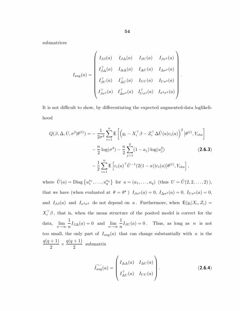
54

submatrices

Iaug(a) =

Iββ(a) Iβ∆(a) IβU (a) Iβσ2(a)

I⊤β∆(a) I∆∆(a) I∆U (a) I∆σ2(a)

I⊤βU (a) I⊤∆U (a) IUU (a) IUσ2(a)

I⊤βσ2(a) I⊤∆σ2(a) I⊤Uσ2(a) Iσ2σ2(a)

.

It is not difficult to show, by differentiating the expected augmented-data loglikeli-

hood

Q(β,∆, U, σ2|θ(t)) = − 1

2σ2

n∑

i=1

E

[(yi −X⊤

i β − Z⊤i ∆U(a)ci(a)

)2 ∣∣θ(t), Yobs

]

− n

2log(σ2) − n

2

q∑

j=1

(1 − aj) log(u2j) (2.6.3)

− 1

2

n∑

i=1

E

[ci(a)

⊤U−1(2(1 − a))ci(a)∣∣θ(t), Yobs

],

where U(a) = Diag{ua1

1 , . . . , uaqq

}for a = (a1, . . . , aq) (thus U = U(2, 2, . . . , 2) ),

that we have (when evaluated at θ = θ⋆ ) Iβσ2(a) = 0, I∆σ2(a) = 0, IUσ2(a) = 0,

and Iββ(a) and Iσ2σ2 do not depend on a . Furthermore, when E(yi|Xi, Zi) =

X⊤i β , that is, when the mean structure of the posited model is correct for the

data, limn→∞

1

nIβ∆(a) = 0 and lim

n→∞

1

nIβU (a) = 0 . Thus, as long as n is not

too small, the only part of Iaug(a) that can change substantially with a is the

q(q + 1)

2× q(q + 1)

2submatrix

Iaug(a) =

I∆∆(a) I∆U (a)

I⊤∆U (a) IUU (a)

. (2.6.4)

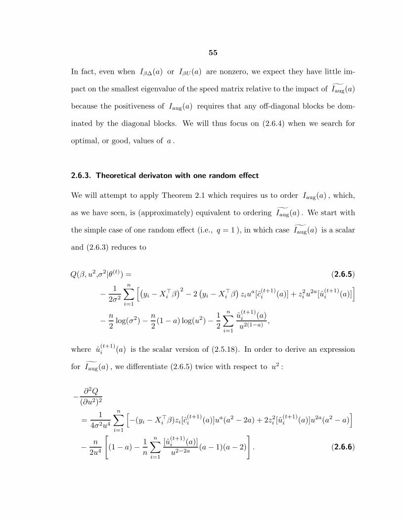
55

In fact, even when Iβ∆(a) or IβU (a) are nonzero, we expect they have little im-

pact on the smallest eigenvalue of the speed matrix relative to the impact of Iaug(a)

because the positiveness of Iaug(a) requires that any off-diagonal blocks be dom-

inated by the diagonal blocks. We will thus focus on (2.6.4) when we search for

optimal, or good, values of a .

2.6.3. Theoretical derivaton with one random effect

We will attempt to apply Theorem 2.1 which requires us to order Iaug(a) , which,

as we have seen, is (approximately) equivalent to ordering Iaug(a) . We start with

the simple case of one random effect (i.e., q = 1 ), in which case Iaug(a) is a scalar

and (2.6.3) reduces to

Q(β, u2,σ2|θ(t)) = (2.6.5)

− 1

2σ2

n∑

i=1

[(yi −X⊤

i β)2 − 2

(yi −X⊤

i β)ziu

a[c(t+1)i (a)] + z2

i u2a[u

(t+1)i (a)]

]

− n

2log(σ2) − n

2(1 − a) log(u2) − 1

2

n∑

i=1

u(t+1)i (a)

u2(1−a),

where u(t+1)i (a) is the scalar version of (2.5.18). In order to derive an expression

for Iaug(a) , we differentiate (2.6.5) twice with respect to u2 :

− ∂2Q

(∂u2)2

=1

4σ2u4

n∑

i=1

[−(yi −X⊤

i β)zi[c(t+1)i (a)]ua(a2 − 2a) + 2z2

i [u(t+1)i (a)]u2a(a2 − a)

]

− n

2u4

[(1 − a) − 1

n

n∑

i=1

[u(t+1)i (a)]

u2−2a(a− 1)(a− 2)

]. (2.6.6)

56

Iaug(a) is equal to (2.6.6) evaluated at θ = θ⋆ , in which case

c(t+1)i (a)ua

∣∣θ=θ⋆ = E[bi|Yobs, θ

⋆] ≡ b⋆i ,

u(t+1)i (a)u2a

∣∣θ=θ⋆ = E[b2i |Yobs, θ

⋆] ≡ τ2⋆i

and1

n

n∑

i=1

τ2⋆i = τ2⋆ , so we may write,

Iaug(a) = (2.6.7)

1

4σ2⋆u4⋆

n∑

i=1

[−(yi −X⊤

i β)zib⋆i (a

2 − 2a) + 2z2i τ

2⋆(a2 − a)]− n

2u4⋆(1 − a)2.

Noting that all the augmented-data normal equations are satisfied for all values of

a at θ = θ⋆ , we evaluate the augmented-data normal equation for u2 with a = 1

at θ⋆ to obtain †

n∑

i=1

z2i τ

2⋆i =

n∑

i=1

zib⋆i (yi −X⊤

i β⋆). (2.6.8)

Substituting (2.6.8) into (2.6.7) yields

Iaug(a) =1

2u4⋆

(a2 1

2σ2⋆

n∑

i=1

z2i τ

2i + (1 − a)2n

). (2.6.9)

Since E[τ2i ] = u2 , we can easily write (2.6.9) in terms of the observed quantities

{(yi, Xi, zi), i = 1, . . . , n} and the maximum likelihood estimate θ⋆ ≡ (β⋆, σ2⋆, u2⋆)

for large n . An even more satisfying result, however, is to rewrite (2.6.9) with-

out appealing to the asymptotic behavior of τ2i . In order to do this we observe

† With q random effects and ∆ assumed to be the identity in model (2.5.13),

this expression can be generalized ton∑

i=1

Z⊤i T

⋆i Zi =

n∑

i=1

Z⊤i b

⋆i (yi −X⊤

i β⋆) , where

T ⋆i is (2.5.3) evaluated at θ(t) = θ⋆ .

57

1

2σ2⋆

n∑

i=1

z2i τ

2⋆i =

1

2σ2⋆

n∑

i=1

zib⋆i (yi −X⊤

i β⋆)

=1

2σ2⋆

n∑

i=1

z2i u

2⋆(yi −X⊤i β

⋆)2

σ2⋆ + z2i u

2⋆

=1

2σ2⋆

[n∑

i=1

(yi −X⊤i β

⋆)2 −n∑

i=1

σ2⋆(yi −X⊤i β

⋆)2

σ2⋆ + z2i u

2⋆

],(2.6.10)

where the first equality is (2.6.8); the second equality follows from the first equation

in (2.5.2) with θ(t) = θ⋆ and q = 1 (in which case T = u and Zi = zi ); and the

third equation follows from substituting (z2i u

2⋆ + σ2⋆ − σ2⋆) for z2i u

2⋆ . To sim-

plify (2.6.10), we use two of the observed-data normal equations∂

∂θ · ∂θ⊤L(θ|Yobs) ,

differentiating first with respect to σ2

∑

i

1

z2i τ

2⋆ + σ2⋆=∑

i

(yi −X⊤

i β⋆

z2i τ

2⋆ + σ2⋆

)2

, (2.6.11)

and then with respect to τ2

∑

i

z2i

z2i τ

2⋆ + σ2⋆=∑

i

(zi(yi −X⊤

i β⋆)

z2i τ

2⋆ + σ2⋆

)2

. (2.6.12)

Adding σ2⋆× (2.6.11) with τ2⋆× (2.6.12) yields ‡

n =∑

i

(yi −X⊤i β

⋆)2

z2i τ

2⋆ + σ2⋆. (2.6.13)

Substituting (2.6.13) into (2.6.10), we may conclude that the augmented information

for u2 given in (2.6.9) is

1

2u4⋆

[a2

(1

2σ2⋆

n∑

i=1

(yi −X⊤i β

⋆)2 − n

2

)+ (1 − a)2n

], (2.6.14)

‡ With q random effects, a similar derivation yields n =

n∑

i=1

(yi −X⊤i β

⋆)2

σ2⋆ + Z⊤i T

⋆Zi,

where T need not be diagonal.

58

which is minimized as a function of a for

aopt =

[∑ni=1(yi −X⊤

i β⋆)2/n

2σ2⋆+

1

2

]−1

.

Unfortunately, implementing the EM algorithm with augmented data Yaug(aopt)

does not result in a simple closed-form M-step unless a ∈ {0, 1} . Thus, although

such an algorithm may converge faster, it does not satisfy our objective of using

algorithms that are simple and stable as well as fast. In what follows, we will

therefore confine our attention to algorithms that result from a ∈ {0, 1} (or, more

generally, for q random effects a ∈ {0, 1}q ). In this class of algorithms, (2.6.14) is

minimized by

aopt =

0 if1

n

n∑

i=1

(yi −X⊤i β

⋆)2 ≥ 3σ2⋆,

1 otherwise.

(2.6.15)

That is, the (small sample) augmented information Iaug(a) is smaller for the new

algorithm (i.e., a = 1 ) than for the standard algorithm (i.e., a = 0 ) if and only if

the total variance is less than three times the residual variance.

2.6.4. Theoretical derivations with q random effects

We now return to the general case of q random effects and will explore how Iaug(a)

depends on a for a ∈ {0, 1}q . We start out by generalizing Iaug(a) (e.g., (2.6.9))

to the case of q random effects. In order to derive I∆∆(a) , we differentiate (2.6.3)

twice with respect to ∆ :

−∂2Q(θ|θ⋆)

∂δlm∂δpr

∣∣∣∣∣θ=θ⋆

=1

σ2⋆

n∑

i=1

zilzip

[U⋆

i

]rm

, (2.6.16)

59

where[U⋆

i

]jk

is the jk th element of E[cic⊤i |Yobs, θ

⋆] , with ci = ∆−1bi . Likewise

we can derive the components of I∆U (a) as

−∂2Q(θ|θ⋆)

∂δlm∂u2p

∣∣∣∣∣θ=θ⋆

=ap

2σ2⋆u2⋆p

n∑

i=1

zil [∆⋆Zi]p

[U⋆

i

]pm

, (2.6.17)

where [∆⋆Zi]j is the j th component of the vector ∆⋆Zi . Finally we derive the

matrix IUU (a) as

−∂2Q(θ|θ⋆)

∂U · ∂U

∣∣∣∣∣θ=θ⋆

= Diag

{(1 − a1)

2 n

2u4⋆1

, . . . , (1 − aq)2 n

2u4⋆q

}

+1

4σ2⋆

n∑

i=1

DiU⋆i Di, (2.6.18)

where Di = Diag

{a1 [∆⋆Zi]1

u2⋆1

, . . . ,aq [∆⋆Zi]q

u2⋆q

}. The task of computing the opti-

mal a is clearly more complicated here than when q = 1 . In fact, we will show

that, in general, we cannot order the information matrices as Theorem 2.1 requires,

even for large n . The problem is somewhat simpler when T is assumed to be

diagonal (i.e., we fit model (2.5.13) with ∆ fixed at the identity). In this case

Iaug(a) reduces to (2.6.18) which can be simplified for large n by re-expressing U⋆i

using (2.5.3) evaluated at θ(t) = θ⋆ (noting that T = U when ∆ = I )

U⋆i = U⋆ +

U⋆ZiZ⊤i U

⋆

σ2⋆ + Z⊤i U

⋆Zi

[(yi −X⊤

i β⋆)2

σ2⋆ + Z⊤i U

⋆Zi− 1

]. (2.6.19)

Thus, if E((yi −X⊤i β)2) = σ2 +Z⊤

i UZi , which is certainly true if the model holds,

limn→∞

1

nIaug(a) =

Diag

{(1 − a1)

2 1

2u41

+ a21

∑ni=1 zi1

4nσ2u21

, . . . , (1− aq)2 1

2u4q

+ a2q

∑ni=1 ziq

4nσ2u2q

}.

Using Theorem 2.1, when T is diagonal, the asymptotic optimal value of a ∈ {0, 1}q

is a such that aj = 0 if and only if

2σ2 ≤u2

j

n

n∑

i=1

[∆Zi]2j . (2.6.20)

60

(We use [∆Zi]j = zij here to make the (2.6.20) easier to generalize to non-diagonal

T .) Condition (2.6.20) says that the standard augmentation should be used on the

j th diagonal component of T if and only if the j th random effect dominates 2σ2 .

Clearly, this result relies heavily on limt→∞ Iaug(a) being diagonal to show

the augmented-data sets are nested. When T is not diagonal, the situation is more

difficult since (2.6.17) involves 1n

∑i[U

⋆i ]jj which remains positive even asymptot-

ically. Suppose, for example, q = 2 , δ⋆21 6= 0 and we choose a′ = (0, 1) and

a = (0, 0) . It can easily be shown that M = limn→∞

[Iaug(a

′) − Iaug(a)]

then

has exactly one positive and one negative eigenvalue, and thus, the augmented-

data sets are not nested. Suppose further that (2.6.20) holds for j = 2 , in which

case we would expect Iaug(a) to be “smaller” than Iaug(a′) and the standard

EM algorithm to be faster. It turns out that whenever a and a′ are of the form

(0, . . . , 0, 1, . . . , 1) , a′ having exactly one less zero than a , the dominate eigenvalue

of M is positive if and only if condition (2.6.20) holds (see Section 2.6.5 for details).

Thus, although (2.6.20) does not assure M will be positive definite, it does indicate

that it will be “more positive than negative”.

We now turn our attention to the relative augmented information R(a′, a =

(0, . . . , 0)) for a′ ∈ {0, 1}q defined in (2.2.2). That is, we will compare each of the

possible algorithms to one that uses Yaug((0, . . . , 0)) , the data augmentation that

most closely approximates the standard algorithm. It is not difficult to show that

61

the diagonal terms of R(a′, a) are

{1, . . . , 1, (1 − a1)

2 + a21

∑ni=1 [∆⋆Zi]

21

[U⋆

i

]11

2nσ2⋆, . . . ,

(1 − aq)2 + a2

q

∑ni=1 [∆⋆Zi]

2q

[U⋆

i

]qq

2nσ2⋆

}

where the ones correspond to the elements of ∆ . Since SEM (a) is fixed, (2.2.2)

indicates that we need to minimize R(a′, a) in order to maximize SEM (a′) . This

suggests that a good choice of data augmentation is Yaug(a′) with

a′j =

0 if 2σ2⋆ ≤ 1

n

n∑

i=1

[∆⋆Zi]2j

[U⋆

i

]jj

,

1 otherwise.(2.6.21)

Notice that asymptotically, this condition corresponds exactly to the optimal value

of a for the diagonal case given in (2.6.20).

The obvious difficulty with the conditions in (2.6.20) and (2.6.21) is that

they depend on the parameter values (unlike the t -model in which the optimal

algorithm is unique). Happily, however, the empirical studies showed that the

standard algorithm is only slightly more efficient when σ2⋆ is small and that using

the new algorithm always will generally lead to great computational advantage and

sometimes will lead to only a slight disadvantage. Moreover, if the optimal algorithm

is desired, a rough approximation of θ⋆ can be used to choose an algorithm as we

discussed in Section 2.6.1.

62

2.6.5. A dominant eigenvalue criterion for choosing an augmented-data set

Given two possible data-augmentation schemes Yaug(a) and Yaug(a′) with

augmented information matrices that have a positive semi-definite ordering (i.e.,

M = Iaug(a′) − Iaug(a) is either positive of negative semi-definite), Theorem 2.1

determines which will result in an EM algorithm with a faster global rate of con-

vergence. Unfortunately, in many cases M is neither positive nor negative semi-

definite. That is M will have both positive and negative eigenvalues. In such cases,

we can define a dominate eigenvalue comparison of two augmented information ma-

trices. In particular, we will say Iaug(a′) ≥eigen Iaug(a) if the dominant eigenvalue

(i.e., largest in absolute value) of M is positive. It is hoped that using this com-

parison in place of the positive semi-definite ordering will give a comparison that

approximates the latter. As we shall see, what this comparison suggests aligns very

well with the simulations presented in Section 2.6.1.

In this section we will consider the augmentations Yaug(a) and Yaug(a′) ,

where a and a′ are such that aj = 0 if j ≤ j0 and 1 otherwise; and a′j = 0

for j ≤ j0 − 1 and 1 otherwise (for some j0 ≤ q ). For example, with q = 3

and j0 = 2 , we would compare a = (0, 0, 1) with a′ = (0, 1, 1) . In this setting

we will show that M = limn→∞1n

[Iaug(a

′) − Iaug(a)]

has exactly one positive

and one negative eigenvalue and that the dominant eigenvalue has the same sign

as∑

i

[∆⋆Zi]2j0

2nσ2⋆− 1

u2⋆j0

. Thus, the asymptotic augmented information matrices do

not have a positive semi-definite ordering, but they may be ordered using the dom-

inant eigenvalue comparison. In particular, we should choose aj = 0 if and only

if 2nσ2⋆ ≤ u⋆j0

∑i [∆⋆Zi]

2j0

, which is identical to condition (2.6.20). Since the or-

63

der of the uj in the information matrix is arbitrary, we may order them so that

u2⋆j

∑i [∆⋆Zi]

2j0

is decreasing in j . In this case, after the q − 1 pairwise compar-

isons resulting from taking j0 = q, q − 1, . . . , 2 , a will be chosen so that aj = 0 if

and only if 2nσ2⋆ ≤ u2⋆j

∑i [∆⋆Zi]

2j for each j , again corresponding to the results

in Section 2.6.4.

It remains to be shown that M has one positive and one negative eigenvalue

with the aforementioned condition on the sign of the dominant eigenvalue, for which

we will need the following lemma.

Lemma : Suppose the (j + k + 1) × (j + k + 1) real matrix M is of the form

M =

0 . . . 0 a1 0 . . . 0...

. . ....

......

. . ....

0 . . . 0 aj 0 . . . 0a1 . . . aj b c1 . . . ck0 . . . 0 c1 0 . . . 0...

. . ....

......

. . ....

0 . . . 0 ck 0 . . . 0

,

then M has one positive and one negative eigenvalue with dominant eigenvalue

having the same sign as b .

Proof: It is easy to show that the characteristic function of M is

λj+k−1

(λ2 − bλ−

j∑

i=1

a2i −

k∑

i=1

c2i

)

and thus M has eigenvalues 0 (with multiplicity j + k − 1 ) and

b±√b2 + 4(

∑ji=1 a

2i +

∑ki=1 b

2i )

2.

Since M is a real symmetric matrix, it has real eigenvalues and the result is clear.

64

From (2.6.16)–(2.6.18) it is clear that M = limn→∞1n

[Iaug(a

′) − Iaug(a)]

has

the form specified by the lemma, so we have proven that if a and a′ are as is

described above, Iaug(a) and Iaug(a′) cannot be ordered in the positive semi-

definite ordering sense but the dominant eigenvalue of M is positive if and only if

u2⋆j0

n∑

i=1

[∆⋆Zi]2j0

≥ 2nσ2⋆ .

Chapter 3

The AECM Algorithm:

Model Reduction and Data Augmentation

3.1. Introduction

With the myriad of models and data structures in modern statistical analysis, max-

imum likelihood estimates and posterior modes are often impossible to ascertain

analytically. Today’s computers, however, offer enough power for many numerical

optimization methods to gain popularity. In this chapter, we will examine two of

these methods, data augmentation in the EM algorithm and model reduction in the

CM algorithm and will show how they can be combined to produce simple, stable

and efficient algorithms.

As we recall, the EM algorithm augments the observed data, Yobs , to the

larger augmented-data set Yaug . It then computes the maximum likelihood esti-

mate θ⋆ as the convergent value of the iteration which sets θ(t+1) to the maximizer

of Q(θ|θ(t)) = E[L(θ|Yaug)|Yobs, θ

(t)]. The idea is to select Yaug so that θ(t+1) is

easy to compute, thereby providing a simple, stable, although sometimes slow algo-

65

66

rithm. The CM algorithm, on the other hand, starts with a set of S ≥ 1 (vector)

constraint functions G = {gs(θ), s = 1, . . . , S} that are “space filling” (Meng and

Rubin, 1993) in the sense of allowing maximization over the entire parameter space.

The algorithm then sets θ(t+ sS

) to the maximizer of L(θ|Yobs) , subject to the con-

straint θ ∈ Θs ≡ {θ ∈ Θ : gs(θ) = gs(θ(t+ s−1

S))} for s = 1, . . . , S . This is repeated

until the algorithm converges to θ⋆ . The idea is to choose G so that each of the

constrained maximizations is easy to implement so as to again produce a simple

algorithm. One common choice of G is the partition {gs(θ) = ϑ2s, s = 1, . . . , S} ,

where ϑ2s is a subvector of θ = (ϑ1s, ϑ2s), s = 1, . . . , S .

Both the ECM (Section 1.3) and SAGE (Section 1.5) algorithms combine

data augmentation and model reduction. ECM starts with EM and adds model

reduction and SAGE starts with CM and adds data augmentation. In particular,

the ECM algorithm starts with EM in cases where although the M-step is not in

closed form, there is a space-filling set of constraints G , such that Q(θ|θ(t)) is

simple to maximize subject to each of the constraints. In such cases, ECM replaces

the M-step of EM with the CM-steps defined by G , that is, one iteration of the

CM algorithm.

The SAGE algorithm, on the other hand, starts with a CM algorithm in

which each of the constraints in G form a partition of θ , but even the constrained

maximizations are not all in closed form. In this case, SAGE uses data augmentation

(i.e., EM) to optimize L(θ|Yobs) over Θs . That is, if a CM-step is not in closed

form, SAGE replaces it with one EM iteration of an algorithm that is designed to

iteratively calculate the maximizer of L(θ|Yobs) over Θs . We interpret SAGE in

67

this way to highlight the fact that since each EM algorithm maximizes L(θ|Yobs)

over a different subspace of Θ , it is natural to adopt a different data-augmentation

scheme for each.

The SAGE algorithm allows for more general data augmentation then does

ECM in that a different data augmentation can be used at each CM-step. On the

other hand, the ECM algorithm is more general than SAGE in that the constraint

functions need not partition θ . Moreover, the MCECM algorithm (a slight gen-

eralization of ECM discussed in Section 1.3) allows additional E-steps to be added

to each ECM iteration, which consists of an E-step followed by S CM-steps, while

the SAGE algorithm must have an E-step preceding each of S CM-step. Thus,

ECM and SAGE generalize EM and CM in different directions. In what follows, we

will develop an algorithm that combines data augmentation and model reduction

in a way that is more general than either ECM or SAGE. The Alternating Expec-

tation/Conditional Maximization or AECM algorithm is built on the intuition of

Dempster, Laird, and Rubin (1977) but, as with ECM, incorporates model reduc-

tion to simplify the M-step; takes advantage of more flexible data augmentation as

in SAGE; and allows some permutation of the component steps within each itera-

tion. In Section 3.2 we will present the details of the AECM algorithm followed by

several convergence results in Section 3.3. Section 3.4 presents an example which

demonstrates how the combination of data augmentation and model reduction in

AECM can be used to develop algorithms that are not only simple and stable, but

also fast.

68

3.2. The AECM Algorithm

To present our algorithm in its most general form, we need to extend and standardize

the indexing system that has been commonly used in the EM literature. Specifically,

we need to develop the concept of a “cycle” in-between a “step” and an “iteration.”

Definition 3.1: A cycle consists of an E-step followed by a ordered set of CM-steps,

the last of which will be followed immediately by a new E-step (which is itself the

beginning of the next cycle). An iteration consists of one or more cycles.

For example, in the ECM algorithm, an iteration is the same as a cycle, but for

MCECM, an iteration consists of multiple cycles (hence its name). In what fol-

lows, we will use t , c , and s to index iteration, cycle, and step, respectively, as

illustrated in the following diagram.

E − step, {CMs step, s = 1, . . . , Sc1}︸ ︷︷ ︸, . . . ,E − step, {CMs step, s = 1, . . . , Sc2

}︸ ︷︷ ︸[ct + 1]th cycle [ct+1]th cycle︸ ︷︷ ︸

tth iteration

The flexibility of our general algorithm comes from allowing the data-augmentation

scheme, as well as the set of constraint functions, to depend on the cycle index.

Because of the alternating nature of the E-step as a consequence of the chang-

ing data-augmentation scheme, we call our algorithm the Alternating Expecta-

tion/Conditional Maximization or AECM algorithm. In the general framework, for

69

cycle c we write Y[c]aug = (Yobs, Y

[c]mis) , where Y

[c]mis is the unobserved part of Y

[c]aug .

For a given c , we select a set of Sc (vector) functions of θ, Gc = {g[c]s (θ), s =

1, . . . , Sc} which induces a sequence of subspaces {Θ[c]s , s = 1, . . . , Sc} of the pa-

rameter space Θ , where Θ[c]s = {θ ∈ Θ : g

[c]s (θ) = g

[c]s (θ[c+

s−1Sc

])} . The [c + 1]st

cycle then consists of

E-step: Compute Qc+1(θ|θ[c]) =

∫L(θ|Y [c+1]

aug )f(Y[c+1]mis |Yobs, θ

[c+1])dY[c+1]mis

and Sc+1 CM-steps

s th CM-step: Calculate θ

[c+ s

Sc+1

]such that

Qc+1(θ

[c+ s

Sc+1

]|θ[c]) ≥ Qc+1(θ|θ[c]) for all θ ∈ Θ[c+1]

s , s = 1, . . . Sc+1. (3.2.1)

The input of the next cycle is taken as θ

[c+

Sc+1Sc+1

]= θ[c+1] .

It is clear that without proper restrictions on the constraint functions,

G[c] = {g[c]s , s = 1, . . . , Sc} , there is no reason to hope that the AECM algorithm

will converge properly. The needed condition here is the space-filling condition

which Meng and Rubin (1993) used for the ECM algorithm. Intuitively, this condi-

tion requires that, after a set of constrained maximizations, we will have searched

in all directions (radiating from a particular origin) of the parameter space. Op-

erationally, the space-filling condition holds for G[c] = {g[c]s , s = 1, . . . , Sc} at a

particular θ′ ∈ Θ if and only if (see Meng and Rubin, 1993)

Sc⋂

s=1

J [c]s (θ′) = {0}, (3.2.2)

where

J [c]s (θ) =

{∇g[c]

s (θ′)λ : λ ∈ Rd[c]

s

}

70

is the column space of the gradient of the d[c]s -dimensional vector g

[c]s (θ) . (We

always assume g[c]s (θ) is differentiable and ∇g[c]

s (θ) is of full rank at each interior

point of Θ to avoid unnecessary technical complications.) For the ECM algorithm,

each iteration consists of one cycle, and G[c] does not depend on the cycle index.

Thus, it was sufficient in Meng and Rubin (1993) to only consider (3.2.2) for one

cycle. With AECM, however, it is possible that the space-filling condition will not

hold for every cycle, that is, it may be useful (for the efficiency of the algorithm)

to allow the space-filling condition to be satisfied only after several cycles. More

precisely, in contrast with (3.2.2), we now only require

c2⋂

c=c1

Sc⋂

s=1

J [c]s (θ′) = {0}. (3.2.3)

For theoretical as well as practical reasons, we will define an iteration of the AECM

algorithm as the smallest set of consecutive cycles such that (3.2.3) holds. More

precisely, we define an AECM iteration sequence {θ(t), t ≥ 0} † as a subsequence

of the sequence generated by the output of each cycle {θ[c], c ≥ 0} such that

θ(t+1) = θ[ct+1] if

ct+1⋂

c=ct+1

Sc⋂

s=1

J [c]s (θ[ct]) = {0}, but

ct+1−1⋂

c=ct+1

Sc⋂

s=1

J [c]s (θ[ct]) 6= {0}. (3.2.4)

In other words, we consider a set of consecutive cycles to form an iteration of the

AECM algorithm if and only if the last cycle of the set has completed the search of

the parameter space, starting from the previous iteration (not cycle) output, in the

sense of completing the space-filling requirement. Since the cycles are time-ordered,

† For clarity, we use parenthesis in the superscript indexing iteration numberand square brackets in the superscript indexing cycle number.

71

there is a unique sequence {ct; t ≥ 0} that defines the iteration sequence. To avoid

the pathological theoretical possibility that there may be only a finite number of ct

which satisfy (3.2.4), we assume the sequence {ct; t ≥ 0} contains infinitely many

distinct numbers.

There are three reasons that call for this definition of an iteration rather

than defining iterations as cycles (e.g., as in Hero and Fessler, 1994). First, the

common notion of an iteration completely updates θ , and thus it is natural to re-

quire that the whole space be searched at each iteration. (Note that even if a cycle

changes the values of all the components of θ , it may not completely update θ ,

as a reparameterization of θ will reveal if the space-filling condition is not satis-

fied.) Second, it is theoretically easier and more satisfactory to study an iteration

mapping from θ(t) to θ(t+1) when the mapping does not depend on t , which for

algorithms that satisfy the space-filling condition, is only possible (in addition to

other requirements) when each of the iterations searches the whole parameter space.

Finally, when monitoring convergence, which is of paramount concern in practice,

the iterates must be comparable. In particular, it is only meaningful to monitor

the difference of consecutive iterates (or functions thereof) when the iterates each

represent a complete update of the parameter rather than just part of it (in which

case one can easily be misled and declare convergence when a small difference is

caused by a small partial update of the parameter).

Table 3.1 provides an overview of how AECM generalizes several existing

algorithms including EM, ECM, SAGE, and ECME (which is given special attention

in Section 3.3.2). In addition to these, there are useful implementations of the

72

AECM Y[c]aug Ct Sc Gc

EM Yaug 1 1 none

ECM Yaug 1 S G

PECM Yaug 1 S {g[c]s (θ) = ϑs}

MCECM Yaug C 1 Gc = Gc mod C

ECME

{Yaug c oddYobs c even

2

{S1 c oddS2 c even

{G1 c oddG2 c even

SAGE Y[c]aug Ct 1 {g[c]

s (θ) = ϑs}

Table 3.1. The special cases of the AECM algorithm. The table records

the data-augmentation scheme (Y[c]aug) , number of cycles per iteration (Ct) ,

number of CM-steps per cycle (Sc) , and constraint functions (Gc) . When

the index c (or t ) is suppressed in the table, the quantity is fixed between

cycles (or iterations). The ECM algorithm introduced model reduction to

EM via the S constraint functions in G . In PECM these constraints have

a special form which partitions θ , that is ϑs is a sub-vector of θ . The

multi-cycle ECM (MCECM) algorithm adds an E-step before each of the

CM-steps. (All of these E-steps need not be added, but then the notation is

more cumbersome.) The ECME algorithm is actually more general than is

presented here in that the S1+S2 CM-steps need not be separated into two

cycles but can be performed in any order. The SAGE algorithm introduced

variable data-augmentation, but updated only one sub-vector of θ at a time.

In Fessler and Hero (1994) an iteration is equivalent to our cycle.

AECM algorithm which are not instances of any of the special cases in Table 3.1.

These include a generalized version of the optimal algorithm of Section 2.3 for

fitting multivariate t -distributions with unknown degrees of freedom, which will be

discussed in Section 3.4.

73

3.3. Convergence Theorems

3.3.1. Convergence of AECM

We now proceed to show that a sequence {θ(t)} of iterates from an AECM algorithm

increases L(θ|Yobs) at each iteration and that under standard regularity conditions,

AECM algorithms converge to a stationary point of L(θ|Yobs) . These results are

the counterparts of the results for EM (Dempster, Laird, and Rubin, 1977; Wu,

1983) and for ECM (Meng and Rubin, 1993), and provide more complete results

for ECME and SAGE.

Our first result, which is most fundamental, states that AECM, like all of its

predecessors, maintains monotonic convergence of the likelihood values. Note that

this result dose not require the space-filling condition.

Theorem 3.1: Any AECM sequence increases (or maintains) L(θ|Yobs) at every

cycle and thus increases (or maintains) L(θ|Yobs) at every iteration.

Proof: The result follows trivially from

Qc+1(θ

[c+ s

Sc+1

]|θ[c]) ≥ Qc+1(θ

[c+ s−1

Sc+1

]|θ[c]), for s = 1, . . . , Sc+1

(as a consequence of (3.2.1)) and the Jensen inequality as used in Dempster, Laird

and Rubin (1977).

In order to prove the algorithm converges to θ⋆ ∈ L = {θ ∈ Θ0 :∂L(θ|Yobs)

∂θ

= 0} where Θ0 is the interior of Θ (i.e., θ⋆ is an interior stationary point), several

regularity conditions similar to the standard ones used by Wu (1983) and Meng

74

and Rubin (1993) for EM and ECM respectively will be required, in particular,

we assume Wu’s (1983) conditions (6) – (10). This is formalized by the global

convergence theorem (c.f., Wu, 1983, Zangwill, 1969) which states that it suffices

to show

(i) The points {θ(t)} are contained in a compact set of Θ ;

(ii) The AECM mapping, θ(t+1) = MAECM (θ(t)) , is closed;

(iii) L(θ(t+1)|Yobs) ≥ L(θ(t)|Yobs) with equality only if θ(t) ∈ L .

The weak inequality in (iii) is an immediate consequence of Theorem 3.1. This,

along with the assumption that the set Θθ(0) = {θ ∈ Θ : L(θ|Yobs) ≥ L(θ(0)|Yobs)}

is compact for any L(θ(0)|Yobs) > −∞ (i.e., Wu’s condition (6)), gives (i). Thus,

it remains only to show (ii) and the equality statement of (iii) hold.

Under Wu’s compactness condition (6) and continuity condition (10), the

same argument used in Meng and Rubin (1993) to show that the ECM mapping,

MECM , is closed can be applied to establish that the mapping determined by each

AECM cycle (i.e., θ[c+1] = MAECM[c] (θ[c]) ) is closed. Since the iteration mapping

θ(t+1) = MAECM(t) (θ(t)) is a composition of several cycle mappings, it is also closed.

Unlike the ECM algorithm where MECM does not change with iteration, however,

an AECM mapping can vary with iteration, and thus, Zangwill’s (1969) global

convergence theorem does not apply directly. Although it is possible to extend

Zangwill’s global convergence theorem to iterate-dependent mappings by imposing

additional regularity conditions, we take a simpler approach by directly requiring

MAECM(t) (θ) not depend on t for t ≥ t0 (typically t0 = 1 ), and hence the simplified

notation given in (ii). The reason we choose to restrict MAECM(t) (θ) in this way

75

is that, although the data-augmentation scheme in AECM varies with cycle and

thus with iteration, the resulting iteration mapping typically remains the same at

each iteration in real applications, as shall be illustrated by our t -model example

in Section 3.4. If useful applications of AECM arise in which MAECM(t) depends on

t , we will develop the more general theory accordingly.

Finally, the equality statement of (iii) can be established using the space-

filling condition in the same way as in the proof of Theorem 2 of Meng and Rubin

(1993) because each AECM iteration contains a complete search of the parameter

space. The only modification needed is to extend (4.5) of Meng and Rubin (1993)

to cover all the cycles contained in one AECM iteration (since ECM contains only

one cycle per iteration) and to note that their (4.3) holds for any Qc(θ|θ[c]), c ≥ 1 .

This completes the proof of the following main result on the convergence of an

AECM iteration sequence {θ(t), t ≥ 0} .

Theorem 3.2: Suppose (a) all the conditional maximizations in (3.2.1) are unique

and (b) the AECM iteration mapping, MAECM(t) : θ(t) → θ(t+1) does not depend

on t , then all the limit points of a AECM iteration sequence {θ(t), t ≥ 0} are

stationary points of L(θ|Yobs).

As discussed in Meng and Rubin (1993), the uniqueness condition (a) is

often satisfied in practice (e.g., when the conditional maximizations are in closed

form), but even this condition can be eliminated if we force θ[c+s

Sc+1 ] = θ[c+s−1

Sc+1 ]

whenever there is no increase in Qc+1(θ|θ[c]) at the s th CM-step within the (c+

1) st cycle. Other conditions are also possible to ensure the result as discussed in

Meng and Rubin (1993). Corollary 1 of Meng and Rubin (1993) also holds here,

76

that is, if L(θ|Yobs) is unimodal with θ⋆ being the only stationary point then under

the conditions of Theorem 3.2, any AECM iteration sequence will converge to the

global maximizer starting from any θ(0) ∈ Θ0 .

Finally, if in addition to assuming that MAECM(t) does not depend on t , we

assume each iteration has the same set of cycles, say {c1, . . . , cC} , we have the

following result regarding the rate of convergence of AECM, the proof of which

is essentially the same as Meng’s (1994) proof of the rate of convergence for the

multi-cycle ECM algorithm.

Theorem 3.3: Suppose the AECM iteration mapping is a composition of C fixed-

cycle mappings, all the conditional maximizations in (3.2.1) satisfy the Lagrange

Multiplier equations, and θ

[c+ s

Sc+1

]→ θ⋆ as c → ∞ . Then the (matrix) rate of

convergence of the AECM iteration is

DMAECM =

C∏

c=1

{I[c]mis

[I [c]aug

]−1

+

(Iobs

[I [c]aug

]−1) Sc∏

s=1

P [c]s

}(3.3.1)

where

I[c]mis =

∫−∂

2 log f(Y[c]mis|Yobs, θ)

∂θ · ∂θ⊤ f(Y[c]mis|Yobs, θ)dY

[c]mis

∣∣∣∣θ=θ⋆

,

I [c]aug =

∫−∂

2 log f(Y[c]aug|θ)

∂θ · ∂θ⊤ f(Y[c]mis|Yobs, θ)dY

[c]mis

∣∣∣∣θ=θ⋆

,

Iobs is given in (1.6.5), and P[c]s = ∇[c]

s

[[∇[c]

s ]⊤[I[c]aug

]−1

∇[c]s

]−1

[∇[c]s ]⊤

[I[c]aug

]−1

with ∇[c]s = ∇g[c]

s (θ⋆) ,∏Sc

s=1 P[c]s = P

[c]1 P

[c]2 · · ·P [c]

Sc, Gc = {g[c]

s (θ), s = 1, . . . , Sc} ,

and Y[c]aug being determined by the c th cycle, c = 1, . . . , C . The global rate of

convergence is governed by the spectral radius of DMAECM .

When C = 1 , the supplemented ECM algorithm (developed in Chapter 4)

uses (3.3.1) to calculate the asymptotic variance-covariance matrix of θ⋆ , I−1obs

77

as a function of DMECM ,∏Sk

s=1 Ps and Iaug . When C > 1 , there is often

a corresponding algorithm with C = 1 which may be less efficient (e.g., SAGE)

for estimating θ⋆ but can be used in conjunction with SECM to calculate I−1obs ,

once θ⋆ has been obtained. This will be further discussed in Section 4.5.2. The

relationship between the spectral radius of DM , the largest eigenvalue of DM ,

and the global rate of convergence will be taken up in Section 5.2.

Theorem 3.3 assumes θ

[c+ s

St+1

]→ θ⋆ , whereas Theorem 3.2 only assures

that θ(t) → θ⋆ . In order to help bridge this theoretical gap we can show that

{θ[c], c ≥ 0} converges to θ⋆ along with its subsequence {θ(t), t ≥ 0} if, in addition

to the assumptions of Theorem 3.2, we assume that for c ≥ c′ , θ[c] ∈ Θ′ , a compact

subset of Θ such that L(θ⋆|Yobs) ≥ L(θ′|Yobs) for all θ′ ∈ Θ′ . This result follows

directly from the following lemma.

Lemma S: Suppose that U is a compact set and f : U →R is a continuous

function with a unique global maximum at x⋆ , so that f(x) < f(x⋆) for any

x ∈ U, x 6= x⋆ . Furthermore, let {xi}∞i=1 be a sequence of points in U such that

the sequence {f(xi)}∞i=1 is nondecreasing and such that there exists a convergent

subsequence {xni}∞i=1 having x⋆ as its limit. Then the entire sequence {xi}∞i=1

converges to x⋆ .

Proof: We first prove that given any ǫ > 0 there exists δ > 0 such that |f(x) −

f(x⋆)| < δ implies |x− x⋆| < ǫ . Suppose otherwise, then, for any natural number

N we could find an xN ∈ U satisfying |f(xN)− f(x⋆)| < 1N while |xN − x⋆| ≥ ǫ .

In this way we obtain a sequence {xN}∞N=1 with each xN ∈ U − Bǫ(x⋆) , which

is also a compact set (where Bǫ(x⋆) is the open ball of radius ǫ and center x⋆ ).

78

Therefore, there exists a convergent subsequence {xNj}∞j=1 whose limit we shall

denote x . Therefore

f(x) = f( limj→∞

xNj) = lim

j→∞f(xNj

) = f(x⋆),

where we have used the continuity of f in the middle step. However, x 6= x⋆ since

|x − x⋆| ≥ ǫ by construction, which contradicts the hypothesis that x⋆ was the

unique point at which f was maximized on U .

So suppose that ǫ > 0 is given. By the above argument we can find δ >

0 such that |f(x) − f(x⋆)| < δ implies |x − x⋆| < ǫ . Since the subsequence

{xni}∞i=1 converges to x⋆ , the sequence {f(xni

)}∞i=1 converges to f(x⋆) since

f is continuous. In particular, we can choose M large enough so that i ≥ M

implies |f(xni)−f(x⋆)| < δ. As f(x⋆) is a maximum this means that f(x⋆)− δ <

f(xni) ≤ f(x⋆) . But by assumption, the entire sequence {f(xi)}∞i=1 is increasing,

so once one of the terms is within δ of f(x⋆) , they all must be. In other words,

|f(xi) − f(x⋆)| < δ for all i ≥ nM , which means that |xn − x⋆| < ǫ , using our

result from the previous paragraph. Since ǫ can be chosen arbitrarily small, we

have proven that

limi→∞

xi = x⋆.

3.3.2. A note on step ordering within ECME

The ECME algorithm takes advantage of a simple idea in order to increase the rate

of convergence of the ECM algorithm. The CM-steps of ECM maximize Q(θ|θ(t))

79

under each of the constraints in G in turn. When it is computationally attractive,

Liu and Rubin (1995a) replace several of these CM-steps with conditional max-

imizations of L(θ|Yobs) (using the same constraint functions) and accomplish a

remarkable increase in the rate of convergence. Unfortunately, there is a technical

error in their proof that an ECME algorithm monotonically increases the likelihood,

which relies on the assertion that the likelihood is increased at each CM-step. This

clearly does not always hold. For an extreme example, consider an ECME algorithm

that, after calculating Q(θ|θ(t)) in the E-step performs one unconstrained maxi-

mization of L(θ|Yobs) followed by one unconstrained maximization of Q(θ|θ(t)) .

Clearly, the output from the second CM-step can decrease L(θ|Yobs) . The prob-

lem stems from the statement in their proof that if Q(θ|θ(t)) increases, so does

L(θ|Yobs) (by Jensen’s inequality), that is

Q(θ|θ(t)) ≥ Q(θ|θ(t)) =⇒ L(θ|Yobs) ≥ L(θ|Yobs), (3.3.2)

which is, in fact, only guaranteed when θ = θ(t).

The AECM algorithm avoids this problem by always calculating θ[c+1] such

that Qc+1(θ[c+1]|θ[c]) ≥ Qc+1(θ

[c]|θ[c]) via a series of CM-steps, each of which

increase Qc+1(θ|θ[c]) . If it is computationally advantageous, L(θ|Yobs) can then

be increased directly via a set of CM-steps in a separate cycle. Put another way,

we always perform an E-step whenever we introduce a different data augmentation.

It should be noted that, although it is easy to find examples of ECME algo-

rithms that do not increase L(θ|Yobs) at each CM-step, we have not yet found an

example of an ECME algorithm that does not increase L(θ|Yobs) at each iteration.

80

It is a proof that ECME (with arbitrary CM-step order) increases the likelihood at

each iteration that we are without.

3.4. Example: Fitting the t-Model with Unknown df

In Section 2.3 we presented an algorithm for fitting the multivariate t -distribution

which is more efficient than the standard iteratively reweighted least squares al-

gorithm when the degrees of freedom are known. Here, we will consider the same

model but with unknown degrees of freedom, a problem that is also of practical

interest (e.g., Lange, Little, and Taylor, 1989). The standard EM algorithm (i.e.,

using the augmentation Yaug = {(yi, qi), i = 1, . . . , n} as described in (2.3.1)) can

be very slow to converge, as Liu and Rubin (1995b) illustrated in their presentation

of the ECME algorithm, which offers great computational gain in this problem. In

this section, we will both extend the optimal algorithm of Section 2.3 to estimate

ν and combine it with the ECME algorithm. We will investigate the performance

of the resulting algorithms empirically and show that the extension of the optimal

algorithm can outperform both the standard algorithm and ECME.

In order to construct the algorithm, we first reduce the model by breaking

the parameter space into two parts in order to use a two cycle algorithm. In the

first cycle, we will update (µ,Σ) given ν , and in the second cycle, we will update

ν given (µ,Σ) . In other words, we choose Θ[c] = {θ ≡ (µ,Σ, ν) ∈ Θ : ν = ν[c−1]}

81

for c odd and Θ[c] = {θ ∈ Θ : (µ,Σ) = (µ[c−1],Σ[c−1])} for c even. The resulting

AECM algorithm has two cycles in each iteration and one CM-step in each cycle

as illustrated below. (We postpone an explicit formulation of Qc+1(θ|θ[c]) and

Qc+2(θ|θ[c+1]) for the moment.) The generic cycle index c here is assumed to be

even.

Odd numbered cycles:

E-step: Compute Qc+1(θ|θ[c])

CM-step: Calculate µ[c+1] and Σ[c+1] such that

Qc+1(θ[c+1] ≡ (µ[c+1],Σ[c+1], ν[c])|θ[c]) ≥ Qc+1(θ|θ[c])

for all θ such that ν = ν[c] .

Even numbered cycles:

E-step: Compute Qc+2(θ|θ[c+1])

CM-step: Calculate ν[c+2] such that

Qc+2(θ[c+2] ≡ (µ[c+1],Σ[c+1], ν[c+2])|θ[c+1]) ≥ Qc+2(θ|θ[c+1])

for all θ such that µ = µ[c+1] and Σ = Σ[c+1] .

The iterations are defined by θ(t) = θ[2t] , and the space-filling condition is easily

satisfied by this algorithm because G1∪G2 partition Θ as in the PECM algorithm

and each iteration uses the same partition G1 ∪G2 .

As was discussed in Section 2.3, there are two choices for the data

augmentation when ν is known (i.e., with the odd numbered cycles) which re-

sult in CM-steps that are simple to compute. The first is the standard aug-

82

mentation {(yi, qi), i = 1, . . . , n} , and the second is the optimal augmentation

{(yi, qi(a[c]opt)), i = 1, . . . , n} , where (yi, qi) is as in model (2.3.1), qi(a) = |Σ|−aqi ,

and a[c]opt = 1/(ν[c] + p) . We see here that since ν[c] changes with c , the op-

timal data augmentation is a function of the cycle, and thus, the resulting algo-

rithm does not fit into the standard EM (or ECM) paradigm. There are also two

data-augmentation schemes when we condition on µ and Σ (i.e., with the even

numbered cycles): the standard augmentation, {(yi, qi), i = 1, . . . , n} , and no aug-

mentation, {yi, i = 1, . . . , n} . The latter was used by Liu and Rubin (1995a) in

their ECME implementation. Since the working parameter a does not affect the

cycle for updating ν[c] , the optimal and standard augmentation are equivalent

when c is even. There are no known data-augmentation schemes that result in

a closed-form update of ν , and both of these data augmentations require similar

computations via a univariate optimization routine.

In conjunction with the standard data augmentation in the odd cycles the

two augmentation schemes in the even cycles result in the MCECM and ECME

algorithms, respectively, and were compared by Liu and Rubin (1995a and 1995b).

Here we compare MCECM and ECME with two new algorithms (AECM 1 and

AECM 2, respectively) which result from replacing the standard augmentation with

the optimal augmentation when updating (µ,Σ) (see Table 3.2). As we shall see,

our simulations indicate that in order to achieve fast algorithms, the choice of data

augmentation when updating (µ,Σ) is more critical than when updating ν .

Implementation of all four algorithms is straightforward. The odd-numbered

cycles are conditional on the current iterate ν[c] and are implemented exactly as

83

Model Reduction (CM-steps): update µ and Σ update ν

Data-Augmentation (E-step): {(yi, qi)} {(yi, qi(a(t)opt)} {(yi, qi)} {(yi)}

MCECM × ×ECME × ×

AECM 1 × ×AECM 2 × ×

Table 3.2. AECM algorithms used to fit the multivariate t with unknown

degrees of freedom. When the degrees of freedom are unknown, it is conve-

nient to first update (µ,Σ) conditional on ν and then update ν condi-

tional on (µ,Σ) . The MCECM algorithm computes the conditional expec-

tation of the augmented-data set {(yi, qi), i = 1, . . . , n} in an E-step before

each of the CM-steps. The ECME algorithm uses only the observed data

to update ν , and the extension of the optimal EM algorithm of Section 2.3

(AECM 1) uses the optimal data-augmentation {(yi, qi(a(t)opt), i = 1, . . . , n}

when updating (µ,Σ) . Using both of these replacements simultaneously re-

sults in the algorithm referred to as AECM 2.

described in Section 2.3 with ν replaced by ν[c] . With the change of notation from

(t+1) to [c+1] , the E-step is given in (2.3.2), and for the standard augmentation,

the CM-step is given in (2.3.3) and (2.3.4). For the optimal augmentation we

replace (2.3.4) with (2.3.6). Regardless of the data augmentation, the even cycles

require numerical optimization of Qc+2(θ|θ[c+1]) , where c is even. Specifically,

when using Yaug = {(yi, qi), i = 1, . . . , n} , we first execute an E-step which sets

w[c+2]i = (ν[c] + p)/(ν[c] + d

[c+1]i ) for each i , and then set ν[c+2] equal to the

solution of the equation:

84

−φ(ν

2

)+ log

(ν2

)+φ

(ν[c] + p

2

)− log

(ν[c] + p

2

)

+1

n

∑

i

[logw

[c+2]i − w

[c+2]i

]+ 1 = 0, (3.4.1)

where φ(·) is the digamma function. Likewise, when using Yaug = {yi, i =

1, . . . , n} , ν is updated by setting ν[c+2] equal to the solution of the equation

−φ(ν

2

)+ log

(ν2

)+φ

(ν + p

2

)− log

(ν + p

2

)

+1

n

∑

i

[log w

[c+2]i − w

[c+2]i

]+ 1 = 0, (3.4.2)

where w[c+2]i = (ν+ p)/(ν+ d

[c+1]i ) . Equations (3.4.1) and (3.4.2) are special cases

of equations (27) and (30) given in Liu and Rubin (1995b).

Although using Yaug = {yi, i = 1, . . . , n} does not require an E-step (since

Yaug is fully observed), it results in a much more costly iteration for updating ν then

Yaug = {(yi, qi), i = 1, . . . , n} since every time (3.4.2) is evaluated during numerical

optimization, the weights w[c+2]i , which depend on ν , must be recomputed and the

function φ(·) must be evaluated twice. Liu and Rubin’s (1995b) simulation shows

that, in their implementation, solving (3.4.2) for ν actually took about seven times

longer than solving (3.4.1) for ν . The hope is that augmenting less will result in

an algorithm that requires fewer iterations for convergence, which will make up for

the extra computational burden per iteration. This was certainly the case in the

examples presented in Liu and Rubin (1995a and 1995b), but as we shall see shortly,

is not the case in our simulations.

In order to compare the performance of the four algorithms described in

85

Table 3.2, we fit a ten-dimensional t -model to 100 observations generated from

t10(0, V, ν = 1) , where V was randomly selected at the outset of the simulation as

a positive definite, non-diagonal matrix. The half-interval method (e.g., Carnahan,

Luther, and Wilkes, 1969) was used to numerically update ν . Using the same

convergence criterion and starting values for (µ,Σ) as described in the simulation

of Section 2.3 and the starting value ν(0) = 10 , the number of iterations required

for convergence was recorded for each of the four algorithms. Figure 3.1 contains

scatter plots which compare AECM 1 to each of the other three algorithms. As we

see, AECM 1 was 8 – 12 times faster than either MCECM or ECME. Remember that

the cost per iteration is less for AECM 1 and MCECM than for ECME. Moreover,

AECM 2 (the combination of the optimal EM algorithm and ECME) was only

slightly more efficient than AECM 1 in terms of the number of iterations required,

and less efficient in terms of actual computer time.

In our simulation the choice of data augmentation when updating ν made

little difference in terms of the number of iterations required for convergence. Yet

Liu and Rubin (1995a and 1995b) have shown that ECME can be much more

efficient than MCECM. There are two principal differences between our simulations

and their examples. Specifically, both of their examples (example 3.1 of Liu and

Rubin 1995a and “artificial example” of Liu and Rubin, 1995b) are two dimensional

(as opposed to ten dimensional in our simulation) and contain much missing data

among the yi , whereas yi was completely observed in our simulations. Figure 3.2

contains the results of a replication of our simulations on two-dimensional data

and again indicates that ECME offers little advantage over MCECM (although the

86

.

.

.

...

..

.

.. .

..

.

.

.

.

. ...

.

. .

.

..

. .

.

..

.

.

.

..

.

.

.

.

.

.

.

.

..

.

.

.

.

.

.

...

.

.

.

.

.

.

.

..

.

.

.

..

.

.

.

.

.

.

.

.

.

.

.

..

.

.

..

..

.

...

.

.

.

.

.

. .

.

.

.

.

.

.

..

.

.

.

..

.

.

..

..

.

.

. .

.

.

.

.

. .

.

.

.

.

..

.

..

.

.

.

.

.

.

..

.

.

.

.

.

.

.

.. .

..

.

.

.

.

. ..

.

..

.

.

.

..

..

.

.

..

...

.

.

..

.

.

.

.

.

.

... .

.

.

.

.

.

. ..

.

.

.

.

.

.

.

.

.

...

..

.

.

..

.

.

.

..

.

.

.

.

.

..

.

. .

.

.

.

.

.

..

.

.

.

.

. .

.

.

.

.

.

...

.

.

.

.

.

.

.

.

.

.

.

.

.

.

.

..

. .

.

...

.

.

.

.

.

. . ..

..

.

.

.

..

.

.

.

.

.

.

..

.

.

.

.

.

.

.

..

.

. .

.

.

.

.

.

.

.

.

.

.

.

.

..

..

.

.

.

..

.

.

.

.

.

. . .

..

.

.

.

.

.. .

.

.

.

.

. ...

.

.

.

..

.

.

.

.

.

.

.

. ..

.

....

.

.

.

.

.

..

. .

. .

.

.

.

.

.

.

.

.

..

.

.

.

....

.

. .

.

.

.

..

..

.

.. .

..

.

.

. ..

.

.

.

.

..

.

.

.

. .

.

.

..

..

.

.

.

.

.

.

...

.

.

.

.

..

. .

.

.

.

.

.

.

.

.

..

.

.

.

.

.

.

..

.

.

.

.

..

.

..

..

.

..

.

.

. .

.

...

.

. .

.

.

..

.

.

.

.

.

.

. .

.

.

..

.

.

.

.

.

.

.

..

...

.

.

.

.

.

.

.

.

.

. ..

..

..

.

.

.

.

.

.

.

.

.

..

...

.

..

.

.

.

. ..

.

.

.

.

.

.

.

.

..

.

.

.

.

..

.

..

..

.

..

.

.

.

..

..

.

.

.

...

..

.

.

.

.

.

.

.

..

.

.

. .

.

.

.

..

.

..

.

..

..

.

.

.

..

.

.

.

.

.

.

.

.

.

.

.

.

.

..

.

.

.

.

.

...

.

.

.

.

.

.

.

.

..

.

. .

.

.

.

.

.

.

.

.

.

.

.

.

.

..

.

.

...

.

.

.

.

.

.

.

.

.

.

.

.

.

. .

.

.

.

.

.

. .

. .

. ...

..

.

..

.

.

.

.

.

.

.

.

.

.

.

.

.

.

.

.

.

.

.

.

.

..

.

.

.

.

.

.

.

..

.

.

.

.

.

...

.

..

.

.

.

.

.

. .

..

..

.

.

..

.

.

...

.

.

.

.

.

.

.

.

.

.

..

.

.

.

.

.

.

.

.

.

.

.

.

.

.

.

.

.

.

.

.

.

.

.

.

.

.

.

.

.

.

.

.

..

.

..

.

.

..

.

.

.

.

. ..

..

..

.

.

.

.

.

.

.

..

.

.

.

.

..

..

.

.

. ..

.

.

.

.

. .

.

.

.

.

.

.

.

.

.

.

..

.

..

.

.

.

.

.

.

.

. ..

.

..

.

.

.

...

.

.

.

.

.

..

.

.

. ..

.

.

.

.

.

.

.

.

.

..

.

.

.

.

..

.

.

.

.

.

.

.

. .

.

.

.

.

.

.

.

.

. .

..

.

.

..

.

.

.

.

.

.

..

. .

.

. .

.

.

.

.

..

.

.

12 14 16 18

100

120

140

160

180

iterations required by AECM 1

itera

tions

req

uire

d by

MC

EC

M

6 times

8 times

10 times

12 times14 times

.

.

.

...

..

.

..

.

..

.

.

.

.

... .

.

..

.

..

. .

.

..

.

.

.

...

.

.

.

.

.

.

.

..

.

.

.

.

.

.

..

.

.

.

.

.

.

.

.

..

.

.

.

..

.

.

.

.

.

.

.

.

.

.

.

..

.

.

..

..

.

. ..

.

.

.

.

.

..

.

.

.

.

.

.

..

.

.

.

..

.

.

..

..

.

.

. .

.

.

.

.

. .

.

.

.

.

..

.

..

.

.

.

.

.

.

..

.

.

.

.

.

.

.

.. .

..

.

.

.

.

. ..

.

..

.

.

.

..

..

.

.

..

...

.

.

..

.

.

.

.

.

.

.

.. .

.

.

.

.

.

. ..

.

.

.

.

.

.

.

.

.

..

...

.

.

..

.

.

.

..

.

..

.

.

..

.

. .

.

.

.

.

.

..

.

.

.

.

. .

.

.

.

.

.

...

.

.

.

.

.

.

.

.

.

.

.

.

.

.

.

..

. .

.

...

.

.

.

.

.

. ...

..

.

.

.

.

.

.

.

.

.

.

.

..

.

.

.

.

.

.

.

..

.

..

.

.

.

.

.

.

.

.

.

.

.

.

..

..

.

.

.

..

.

.

.

.

.

. ..

..

.

.

.

.

.. .

.

.

.

.

. ..

.

.

.

.

..

.

.

.

.

.

.

.

. ..

.

....

.

.

.

.

.

..

..

. .

.

.

.

.

.

.

.

.

..

.

.

.

..

..

.

. .

.

.

.

..

..

.

.. .

..

.

.

. ..

.

.

.

.

..

.

.

.

. .

.

.

..

..

.

.

.

.

.

.

.. ..

.

.

.

..

..

.

.

.

.

.

.

.

.

..

.

.

.

.

.

.

..

.

.

.

.

..

.

..

..

.

..

.

.

. .

.

...

.

. .

.

.

..

.

.

.

.

.

.

. .

.

.

..

.

.

.

.

.

..

..

...

.

.

.

.

.

.

.

.

.

...

..

..

.

.

.

.

.

.

.

.

.

.

.

..

.

.

.

.

.

.

.

. ..

.

.

.

.

.

.

.

.

..

.

.

.

.

..

.

..

..

.

..

.

.

.

..

..

.

.

.

.. ..

.

.

.

.

.

.

.

.

..

.

.

. .

.

.

.

..

.

..

.

..

..

.

.

.

..

.

.

.

.

.

.

.

.

.

.

.

.

.

..

.

.

.

.

.

...

.

.

.

.

.

.

.

.

..

.

..

.

..

.

.

.

.

.

.

.

.

.

.

..

.

.

...

.

.

.

.

.

.

.

.

.

.

.

.

.

. .

.

.

.

.

.

. .

. .

. ...

..

.

..

.

.

.

.

.

.

.

.

.

.

.

.

.

.

.

.

.

.

.

.

.

..

.

.

.

.

.

.

.

..

.

.

.

.

.

...

.

..

.

.

.

.

.

. .

..

..

.

.

. .

.

.

..

.

.

.

.

.

.

.

.

.

.

.

..

.

.

.

..

.

.

.

.

.

.

.

.

.

.

.

.

.

.

.

.

.

.

.

.

.

.

.

.

.

.

.

..

.

..

.

.

..

.

.

.

.

. ..

..

.

.

.

.

.

.

.

.

.

..

.

.

.

.

.

.

..

.

.

. ..

.

.

.

.

. .

.

.

.

.

.

.

.

.

.

.

..

.

..

.

.

.

.

.

.

.

. ..

.

..

.

.

.

..

.

.

.

.

.

.

..

.

.

. ..

.

.

.

.

.

.

.

.

.

..

.

.

.

.

..

.

.

.

.

.

.

.

. .

.

.

.

.

.

.

.

.

. .

..

.

.

..

.

.

.

.

.

.

..

. .

.

. .

.

.

.

.

..

.

.

12 14 16 18

100

120

140

160

180

200

iterations required by AECM 1

itera

tions

req

uire

d by

EC

ME

6 times

8 times

10 times

12 times14 times

..

.

...

...

.

.

.

.

.. ..

.

.

..

.

.

.

.

.

.

.

.

. ..

.

.

. .

.

.. ..

.

.

.

.

.

..

.

.

.

.

.

.

. ..

.

.

.

.

.

...

.

.

.

.

.

..

.

.

.

.

.

..

.

.

.

.

.

.

.

.

.

. ..

.

.

.

.

. ..

.

. .

..

.

.

..

.

.

.

.

.

.

.

.

.

..

.

.

. .

.

. .

.

.

.

.

.

.

.

. .. .

.

.

.

.

.

..

.

.

.

.

.

..

.. .

.

..

.

.. ...

.

.

.

..

.

..

.

..

.

.

..

.

.

..

..

..

..

.

.

.

.

.

..

.

.

.

.

.

.

.

.

.

..

.

.

.

.

.

.

.

.

.

..

.

.

.. .

.

..

.

.

..

.

..

.

.

.

.

.. . ...

.

.

.

.

.

.

.

.

.

.

.

.

.

.

.

.

.

..

.

.

..

..

.

.

.

.

.

.

.

..

.

.

.

.

.

.

.

.

...

..

.

.

... . .

..

. ..

.

.

. .

..

.

.

.

.

.

..

. .

.

.

.

.

.

.

.

.

.

.

..

.

..

.

.

. .

.

.

.

.

.

.

.

.

.

.

.

.

.

... .

.

.

.

. .

.

.

.

.

.

.. .

..

..

.

.

.

.

.

.

.

.

. .

.

.

.

..

.

.

....

... .

. .

..

.

.

.

.

.

.

.

.

.

.

.

.

.

.

. .

.

.. .

.

..

..

.

.

. .

..

.

.

. .

.

.

..

.

.

.

.

.

.

. .

.

.

. .

..

..

..

.

.

.

.

... ..

.

.

.

.

.

.

.

.

.

.

.

..

.

.

. .

.

. .

.

..

. .

.

.

....

.

.

.

.

.

. .

.

.

..

.

.

.

.

.. .

..

.

.

.

.

.

.

.

..

. .

.

. .

.

.

.

.

.

.

.

.

.

.

.

.

.. .

..

.

.

.

..

.

..

.

..

.

.

.. .

.

.

.

.

..

...

.

..

..

.

.

.

.

. . .

.

.

..

.

..

.

.

.

.

.

.

.

.. ..

.

.

.

. ..

.

.

.

.

.

.

. .

.

.

.

.

..

.

.

.

.

.

. ..

..

.

..

.

. .

.

.

.

.

.

.

.

. .

..

.

.

.

.

.

.

.

.

.

.

.

. .

.

.

.

. .

.

.

..

.. .

.

.

. .

.

. . .

.

.

.

.

..

.

.

.

.

.

.

..

.

.

.

.

.

.

.

..

.

.

.

.

. .

.

.

.

.

.

. ..

.

.

..

. .

.

..

. . ..

..

. .

.

. ..

.

.

.

.

.

.

.

.

.

.

.

.

.

. .

.

.

.

..

.

.

..

. .

.

.

..

..

..

.

.

.

. .

.

.

.

..

.

.

.

.

..

... .

..

.

.

.

.

. ..

.

. ..

.

.

..

.

.

.

.

..

.. .

..

.

.

.

..

. .

.

.

.

.

.

.

.

.

.

.

.

.. .

.

...

.

.

.

.

..

.

.

. .

.

.

.

.

..

.

.

.

.

.

.

. .

.

.

. .

.

. .

.

.

..

.

.

.

. ..

. .

..

.

.

.

.

..

.

. .

.

.

.

.

.. .

.

.

.

.

.

.

.

.

.

..

.

.

.

...

.

.

.

.

.

..

.

.

.

.

. . .

. ..

.

.

.

...

.

..

.

.

.

.

.

..

.. ..

.

.

.. .

.

.

.

.

.

.

.

.

. .

.

..

.

.

.

.

.

.

.

...

.

.

.

.

.

.

.

.

.

.

.

.

12 14 16 18

1214

1618

iterations required by AECM 1

itera

tions

req

uire

d by

AE

CM

2

equal

Figure 3.1. Comparing AECM algorithms for fitting the multivariate twith unknown degrees of freedom. The scatter plots compare the num-

ber of iterations required for convergence by each of MCECM, ECME, and

AECM 2 with AECM 1 respectively. AECM 1 and 2 use the optimal data-

augmentation of Section 2.3 for (µ,Σ) and perform very well. ECME and

AECM 2 use Yobs in place of Yaug when updating ν and show only a small

improvement over MCECM and AECM 1 respectively. This improvement

is washed out by the increased computation time required per iteration by

AECM 2

87

.

.

.

.

.. .

.

.

.

.

.

..

.

..

.

.

.

.

.

..

.

.

.

.

.

.

.

.

.

..

..

.

.

..

.

.

.

.

.

.

.

.

.

.

..

.

..

.

.

. .

.

.

.

.

.

.

.

..

.

...

.

.

.

.

.

.

...

.

.

.

..

..

.

.

.

.

.

. .

.

.

... ..

.

..

.

.

.

.

.

.

.

.

..

.

.

...

.

..

.

.

.

.

.

..

.

.

..

.

..

.

. .

.

.

.

.

.

.

..

..

.

..

.. ..

..

.

.

.

...

. ..

.

.

.

. .

... ..

.

..

.

.

.

.

.

.

.

.

.

.

. .

.

.

..

.

.

.

.

.

.

.

.

.

. ..

.

.

.

.

.

.

..

.

.

.

.

. ..

.

.

.

.

.

.

.

.

.

.

.

..

.

.

.

..

. .

.

.

..

.

.

. ..

.

.

.

.

..

.

.

.

.

.

.

.

.

.

...

.

.

.

.

.

.

.

.

.

.

.

. .

.

.

.

.

.

.

.

.

.

..

.

.

.

..

.

. . ..

.

.

.

.

.

.

.

.

.

.

..

.

.

.

.

.

.

.

.

.

.

.

.

.

.

.

.

.

.

.

.

. ...

.

..

.

.

.

.

..

..

.

.

.

..

.

.

.

.

..

.

.

..

.

.

..

...

. .

..

..

..

.

.

.

.

.

..

.

.

.

..

.

.

.

.

.

.

.

.

...

.

.

.

.

.

..

.

. ..

..

..

.

.

.

..

.. .

.

.

.

.

.

.

. .

.

..

.

.

.

.. ..

.

.

.

..

.

.

. .

.

.

.

.

.

.

..

.

.

.

.

.

..

.

. . .

..

.

.

.

.

.

.

.

..

.

.

.

.

.

. .

.

.

.

.

..

.

..

.. .

.

. ..

.

.

.

.

...

.

..

.

.

.

..

.

.

.

. .

.

..

.

..

...

.

.

..

.

.

..

.

.

.

.

. ..

.

.

.

.

.

. ..

..

. .

.

.

.

.

.

.

.

.

.

.

.

.

.

.

.. ..

.

.

. .

.

. .

.

.

.

.

.

.

.

.

.

..

.

..

.

.

.

.

.

....

.

..

.

.

.

.

.

.

..

.

.

.

..

.

.

.

..

.

.

..

.

..

..

.

.

.

.

.

.

..

.

.

.

.

.

.

. .

..

.

.

..

.

.

. .

.

.

..

.

.

.

.

.

.

.

.

.

..

.

.

. .

..

.

.

.

.

.

.

..

.

.

.

.

.

. ...

.

.

..

...

.

.

.

.

.

.

..

.

.

.

.

..

.

.

..

.

.

...

.

.

.

.

.

.

.

.

.

..

. .

.

.

.

.

.

.

.

...

.

.

.

.

.

.

. .

.

.

.

.

.

.

.

.

.

..

.

.

.

.

.

.

..

.

.

.

. .

.

.

.

. .

.

....

.

.

.

.

.

..

..

.. .

..

.

.

..

.

.

..

.

.

.

.

.

.

.

.

.

..

.

.

..

..

.

.

.

...

.

.

..

.

.

.

.. .

.

.

.. .

. .

.

.

.

.

.

.

.

.

. .

.

. .

.

.

.

..

..

.

..

..

.

.

..

.

..

.

..

.

.

.

.

. .

..

.

.

.

.

.

.

.

.

... .

.

.

. .

.

.

.

.

.

. .

.

.

.

.

.

.

. ..

.

.

.

.

.

.

.

.

.

..

.

.

.

.

.

. .

..

.

.

.

.

.

.

.

..

..

..

.

. ..

.

..

.

.

.

.

.

.

.

.

.

. ..

.

.

.

..

.

.

.

.

20 25 30 35 40

5060

7080

9010

0

iterations required by AECM 1

itera

tions

req

uire

d by

MC

EM

C

2 times

3 times4 times

.

.

.

.

.. .

.

.

.

.

.

..

.

..

.

.

.

.

.. .

.

.

.

.

.

.

.

.

.

..

.

..

.

. .

.

.

.

.

.

.

.

.

.

.

..

.

..

.

.

. .

. .

.

.

.

.

.

.

.

.

... .

.

.

.

.

.

.

..

.

.

.

..

....

.

.

.

. .

.

.

. .. ..

..

..

.

.

.

.

.

.

.

..

.

.

..

.

.

..

.

.

.

.

.

..

.

.

.

.

.

..

.

. .

.

.

.

.

.

.

..

.

.

.

..

...

.

..

.

.

.

... .

..

.

..

. .

...

.

.

.

..

.

.

.

.

.

.

.

.

.

.

. .

.

.

..

.

.

.

..

.

.

.

.

. ..

.

.

.

.

.

.

..

.

.

.

.

..

.

. .

.

.

.

.

.

.

.

.

.

..

.

.

.

... .

.

.

..

.

.

. ..

.

.

.

.

..

.

.

.

.

.

.

.

.

.

...

.

.

.

.

.

.

.

.

.

.

.

. .

.

.

.

.

.

.

.

.

.

..

.

.

.

..

.

. . ..

.

.

.

.

.

.

.

.

.

.

..

.

.

.

.

.

..

.

.

.

.

.

.

.

.

.

.

.

.

.

..

..

.

..

.

.

.

.

..

. .

.

.

.

..

.

.

.

.

. .

.

.

. .

.

.

.

.

....

.

.

..

.

...

.

.

.

.

..

.

.

.

..

.

.

.

.

.

.

.

.

...

.

.

.

.

.

..

.

..

.

..

. .

.

.

.

..

. .

.

.

.

.

.

.

.

. .

.

.

.

.

.

.

.

...

.

.

.

..

.

.

. .

.

.

..

.

.

..

.

..

.

.

.

.

.

. . .

..

.

.

.

.

..

.

.

..

.

..

.

. .

.

.

.

.

.

.

.

.

... .

.

. .

.

.

.

.

.

...

.

..

.

.

.

.

.

.

.

.

. .

.

.

.

.

..

..

.

.

.

..

.

.

..

..

.

.

...

.

.

..

.

. ..

.

.

..

.

.

.

.

.

.

.

.

.

.

.

.

.

.

.. .

.

.

.

. .

.

. .

.

.

.

.

.

.

.

.

.

..

.

..

.

.

.

.

.

....

.

.. .

.

.

.

.

.

..

.

.

.

.

.

.

.

.

..

.

.

.

.

.

..

.

.

.

.

.

.

.

.

..

.

.

.

..

.

. .

..

.

.

.

..

.

. .

.

.

..

.

.

.

.

.

..

.

.

.

.

.

.

. .

..

.

.

.

.

.

.

..

.

.

.

.

.

. ...

.

..

.

...

.

.

.

.

.

.

. ..

..

.

..

.

..

.

.

.

...

.

.

.

.

.

.

.

.

.

.

.

. .

.

.

.

.

.

.

.

...

.

.

.

.

.

.

. .

.

.

.

.

.

.

.

.

.

..

.

.

.

.

.

.

..

.

.

.

. .

.

.

.

.

.

.

....

.

..

.

.

.

.

..

..

.

..

.

.

..

.

.

..

.

.

.

.

.

.

.

.

.

.

.

.

.

..

..

.

.

.

.. .

.

.

..

.

.

... .

.

.

.. .

..

.

.

.

.

.

.

.

.

.

.

.

. .

..

.

..

..

.

..

.

.

.

.

. .

.

.

.

.

. .

.

.

.

.

..

..

.

.

.

.

.

.

.

.

.

.. .

.

.

. .

.

.

.

.

.

. ..

.

.

.

.

.. .

..

.

.

.

.

.

.

.

.

..

.

.

.

.

.

..

.

.

.

.

.

.

.

.

.

..

..

..

.

. ..

.

..

.

.

.

.

..

.

.

.

. ..

.

.

.

.

. ..

.

.

20 25 30 35 40

4050

6070

8090

100

iterations required by AECM 1

itera

tions

req

uire

d by

EC

ME

2 times

3 times4 times

.

.

.

.

..

.

.

. ..

.

.. .

.

.

.

.

..

.

.

..

.

....

.

.

.

.

.

.

...

.

..

.

.

.

.

.

.

.

.

.

... .

.

.

.

.

.

.

.

.

.

.

.

..

.

.

.

.. .

.

..

.

.

.

..

.

.

..

.

.

.

.

..

.

.

..

..

.

.. .

. .

.

.

.

.

.

.

..

..

.

.

.

.

...

.

...

.

.

.

.

..

.

.

.

.

.

. ..

.

..

.

.

.

.

.

.

.

.

. .

...

.

.

.. .

.

.

. ..

.

.

.

. .

.

.

. .

.

.

.

. .

. .

.

.

.

.

..

..

.

..

.

..

..

..

.

.

.

.

.

.

.

. ..

.

.

.

.

.

.

.

.

.

.

.

.

.

. .

. .

.

.

.

..

.

.

.

.

.

..

..

..

..

.

.

.

.

.

.

.

.

.

. ..

.

.

..

.

.

.

..

..

.

....

. .

. .

.

.

.

.

.

.

..

.

.

.

.. .

.

.

.

.

. .

.

.

.

..

.

.

.

.

. ...

. ..

.

.

.

.

.

.

.

.

.

.

.

.

.

.

.

.

..

.

..

.

.

..

..

.

..

.

..

.

.

..

..

. .

.

.

.

.

.

..

.

.

.

.

.

.

.

.

.

.

..

..

.

.

.

.

.

.

.

..

.

....

..

.

..

.

.

. .

..

.

.

.

.

.

.

.

..

..

.

...

.

..

.

..

.

..

.

.

..

..

.

.

.

.

.. .

. .

..

.

.

.

..

.

..

. .

..

...

. ..

.

.

.

.

..

.

.

.

.

.

.

.

.

..

.

.

..

..

.

.

.

.

. .

.. ..

.

. .

.

.

.

.

..

.

...

.

.

.

.

.

.

.

.

.

.

.

.

.

....

.. .

.

.

.

.

. .

.

.

.

.

. ...

.

.

..

.

.

.

..

.

.

.

.

.

..

..

.

.

. ..

.

.

.

.

.. .

.

.

.

.

.

..

.

. ... .

.

.

.

..

. .

..

. .

.

.

.

.

.

.

.

.

.

.

.

.

...

.

...

.

..

..

.

.

.

.

.

..

.

.

.

.

.

. ...

.

..

.

.

.

.

. .

.

. .. .

.

.

.

.

..

.

.

.

.

.

...

..

..

..

..

.

.

.

.

..

.

.

...

.

.

.

.

.

...

.

.

. . .

.

.

.

.

.

.

. .

.

...

.

...

.

.

.

...

..

.

.

.

...

.

.

....

.

.

.

.

.

. .

.

..

.

.

..

.

.

. ... ..

..

..

.

.

. .

.

..

.

..

.

.

.

.

.

..

.

.

..

.

.

.

.

.

.

. ..

.

. ..

.

.

.

.

.

.

.

.

.

.

.

.

...

.

.

.

.

.

.

.

..

.

.

.

.

.

.

.

.

.

..

..

.

..

.

.

..

.

.

.

..

.

.

.

. .

.

.

.

..

.

.

.

.

.

.

. .

.

.

.

.

.

.. .

.

.

.

.

.

.

..

.

.

.

..

.

.

.

. .

.

. ..

.

..

.

.

. .

. .

.

.

.

.

..

. .

.

.

.

.

..

.

.

.

.

.

.

.

.

.

..

..

..

..

.

.

.

.

. .

.

.

.

.

.

.

.

.

.

.

.. .

. .

..

.

.

.

..

.

...

.

.

.

.

.

.

.

.

.

.

..

.. ...

.

.

.

.

.

.

.

.

..

.

.

..

.

..

.

.

.

. ..

..

. .

20 25 30 35 40

2025

30

iterations required by AECM 1

itera

tions

req

uire

d by

AE

CM

2

equal

half

Figure 3.2. Comparing AECM algorithms for fitting the bivariate t with

unknown degrees of freedom. The scatter plots compare the number of iter-

ations required for convergence by each of MCECM, ECME, and AECM 2

with AECM 1 respectively. The computational gain of not augmenting when

updating ν is again dwarfed by the gain of using the optimal augmentation

for (µ,Σ) .

88

improvement is somewhat greater than in the 10 dimensional case). Thus, it seems

that when fitting t -models, ECME is most useful when there is much missing data

among the yi . How this interacts with the optimal augmentation for (µ,Σ) has

yet to be investigated.

Chapter 4

The SECM Algorithm:

Computing the Asymptotic Variance

4.1. Introduction

In the previous chapter we discussed how the AECM algorithm can be used to

compute maximum likelihood estimates in the presence of missing data. Generally,

statistical inference requires not only point estimates but also measures of uncer-

tainty, for example (asymptotic) variance-covariance matrix of the estimates. The

Supplemented EM (SEM) algorithm (Meng and Rubin, 1991a) computes such ma-

trices using a sequence of EM iterates to obtain the matrix rate of convergence

of EM. This rate is then used to inflate the augmented-data asymptotic variance-

covariance matrix to obtain the asymptotic variance matrix for the observed-data

MLEs. A key feature of SEM is that it requires only the code for EM and the code

for computing the augmented-data asymptotic variance-covariance matrix.

In this chapter we develop and illustrate an analogous supplemented algo-

rithm for ECM, SECM, which computes the asymptotic variance-covariance matrix

89

90

of the MLEs. In addition to requiring the computation of both the rate of con-

vergence of ECM and the augmented-data variance-covariance matrix, it requires

the computation of the rate of convergence of the CM algorithm. The computa-

tions of SECM, however, remain as simple as SEM in the sense that they only

require the ECM code along with the code for computing the augmented-data

variance-covariance matrix. Although our presentation is focused on the asymp-

totic variance-covariance matrix of the MLEs, the SECM algorithm can just as

easily be applied to compute the asymptotic posterior variance-covariance matrix

when ECM is used to find a posterior mode, which includes penalized likelihood

models as a special case (e.g., Segal, Bacchetti, and Jewell, 1994).

After reviewing the SEM algorithm and other necessary theoretical develop-

ment in Section 4.2, in Section 4.3 we detail the computational steps of SECM.

Section 4.4 presents four examples to illustrate a variety of applications of the

SECM algorithm. Section 4.5 offers discussion on some practical issues involved in

implementing SECM, in particular, we will discuss the computation of asymptotic

variance-covariance matrix when other EM-type algorithms are implemented.

4.2. Methodological Development

4.2.1. The SEM algorithm

The EM algorithm, as described in Section 1.2 is designed to calculate θ⋆ the maxi-

mizer of the observed-data loglikelihood L(θ|Yobs) = log f(Yobs|θ) . The SEM algo-

91

rithm supplements the EM algorithm in order to calculate the asymptotic variance-

covariance matrix of (θ − θ⋆) , that is, I−1obs , which is defined in (1.6.5). The

algorithm is based on the fundamental identity, DMEM = ImisI−1aug , as presented

in (1.6.2). This identity underlies the SEM computations because the desired infor-

mation matrix, Iobs , can be written as the difference between the augmented and

missing information (e.g., Orchard and Woodbury, 1972; Meng and Rubin, 1991a)

Iobs = Iaug − Imis = [Id − ImisI−1aug]Iaug = [Id −DMEM ]Iaug, (4.2.1)

where Id is the d× d identity matrix. In other words, to compute Iobs , we need

only compute DMEM and Iaug . When the augmented-data model, f(Yaug|θ)

is from the exponential family, as is typically the case when the E-step is com-

putable, Iaug = Io(θ⋆|S⋆(Yobs)), where S⋆(Yobs) = E(S(Yaug)|Yobs, θ

⋆) , as found

at the last E-step; we thus can compute Iaug using standard augmented-data pro-

cedures. Computing DMEM can be accomplished by numerical differentiation of

the EM mapping. Details of these SEM calculations are provided in Meng and

Rubin (1991a) and will be reviewed in Section 4.3 .

4.2.2. The matrix rate of convergence of CM and ECM

To apply the logic of the SEM procedure to ECM, we need to relate the matrix

rate of convergence of ECM to the fraction of missing information. Meng (1994)

extended (1.6.2) to the ECM case with the following result:

[Id −DMECM ] = [Id −DMEM ][Id −DMCM ], (4.2.2)

where DMECM is the rate of convergence of ECM at θ = θ⋆ , and DMCM is

92

the rate of convergence of CM at θ = θ⋆ . If we knew DMECM and DMCM , we

could use (4.2.2) and (4.2.1) to calculate the asymptotic variance, Vobs ≡ I−1obs .

As will be detailed in Section 4.3, DMECM can be computed by numerical

differentiation just like DMEM . The rate of CM, DMCM , can be computed in

two ways. Meng (1994) shows that it can be calculated analytically as given in

(1.6.7) and (1.6.8). All the quantities in (1.6.7) involve only the augmented-data

information matrix and the g functions, and thus, they can be computed once θ⋆

is obtained.

Alternatively, when the augmented-data model f(Yaug|θ) is from an expo-

nential family, DMCM can be obtained numerically from the output of ECM at

convergence, (θ⋆, S⋆(Yobs)), and an additional run of the code for the CM-steps. If

we take S⋆(Yobs) to be the fixed augmented-data sufficient statistics, we can obtain

θ(S⋆(Yobs)) , the MLE of θ given S⋆(Yobs) , using the CM algorithm starting from

θ(0) 6= θ⋆ ; DMCM is the rate of convergence of this CM algorithm. This can be

proved by examining (1.6.8) and noting that if f(Yaug|θ) is from an exponential

family, Iaug = Io(θ⋆|S⋆(Yobs)) and that θ⋆ = θ(S⋆(Yobs)) . Thus, we can derive

DMCM by calculating the rate of convergence of the CM algorithm applied to

L(θ|S⋆(Yobs)) . This avoids the matrix inversions and computation of the ∇s in

(1.6.7) and (1.6.8), which are necessary when performing analytical calculations.

With the PECM algorithm described in Section 1.3, the computation of

DMCM is particularly easy. Let Υ be the block diagonal matrix of Iaug with S

blocks corresponding to the S subvectors of θ defined by the partition. Let Γ be

the corresponding lower block triangular matrix of Iaug , that is, Iaug = Υ+Γ+Γ⊤.

93

Meng (1990) established that in this case (1.6.7) reduces to

DMCM = −Γ[Υ + Γ⊤]−1, (4.2.3)

which makes analytical calculation of DMCM very simple, as illustrated in Sec-

tion 4.4.2.

4.2.3. The basic identity for the SECM algorithm

Having obtained DMECM , DMCM , and Iaug , we can combine (4.2.1) and (4.2.2)

to obtain

Iobs = Io(θ⋆|Yobs) = [Id −DMECM ][Id −DMCM ]−1Iaug. (4.2.4)

Equivalently, in terms of the variance,

Vobs ≡ I−1obs = Vaug + ∆V, (4.2.5)

where Vaug = I−1aug can be viewed as the variance-covariance matrix of the MLE

given the augmented data, and

∆V = Vaug[DMECM −DMCM ][Id −DMECM ]−1 (4.2.6)

is the increase in variance due to the missing data.

Identity (4.2.6) is the basis for the SECM algorithm, and it reduces to (2.3.6)

of Meng and Rubin (1991a) when DMCM = 0 , which corresponds to EM. An

interesting property of SECM (and SEM) is that, although ∆V is mathematically

symmetric, the right side of (4.2.6) is not numerically constrained to be symmetric

because Vaug , DMCM , and DMECM are computed separately as described in

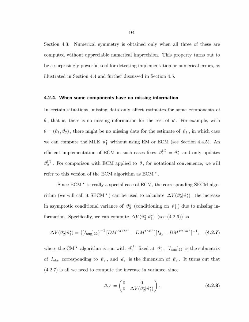
94

Section 4.3. Numerical symmetry is obtained only when all three of these are

computed without appreciable numerical imprecision. This property turns out to

be a surprisingly powerful tool for detecting implementation or numerical errors, as

illustrated in Section 4.4 and further discussed in Section 4.5.

4.2.4. When some components have no missing information

In certain situations, missing data only affect estimates for some components of

θ , that is, there is no missing information for the rest of θ . For example, with

θ = (ϑ1, ϑ2) , there might be no missing data for the estimate of ϑ1 , in which case

we can compute the MLE ϑ⋆1 without using EM or ECM (see Section 4.4.5). An

efficient implementation of ECM in such cases fixes ϑ(t)1 = ϑ⋆

1 and only updates

ϑ(t)2 . For comparison with ECM applied to θ , for notational convenience, we will

refer to this version of the ECM algorithm as ECM ⋆ .

Since ECM ⋆ is really a special case of ECM, the corresponding SECM algo-

rithm (we will call it SECM ⋆ ) can be used to calculate ∆V (ϑ⋆2|ϑ⋆

1) , the increase

in asymptotic conditional variance of ϑ⋆2 (conditioning on ϑ⋆

1 ) due to missing in-

formation. Specifically, we can compute ∆V (ϑ⋆2|ϑ⋆

1) (see (4.2.6)) as

∆V (ϑ⋆2|ϑ⋆

1) = {[Iaug]22}−1[DMECM⋆ −DMCM⋆

][Id2−DMECM⋆

]−1, (4.2.7)

where the CM ⋆ algorithm is run with ϑ(t)1 fixed at ϑ⋆

1 , [Iaug]22 is the submatrix

of Iobs corresponding to ϑ2 , and d2 is the dimension of ϑ2 . It turns out that

(4.2.7) is all we need to compute the increase in variance, since

∆V =

(0 00 ∆V (ϑ⋆

2|ϑ⋆1)

). (4.2.8)

95

This identity holds because (i) there is no increase in variance or covariance of ϑ⋆1

and (ii) there is no increase in the part of the variance of ϑ⋆2 that can be explained

by ϑ⋆1 (see Meng and Rubin, 1991a). When there is no missing information for ϑ1 ,

we can therefore calculate ∆V using (4.2.8) and then calculate Vobs using (4.2.5).

It is, however, worth remarking that fixing ϑ(t)1 at ϑ⋆

1 increases the efficiency of

ECM and SECM but is not a required step since the standard ECM and SECM

algorithms will produce the desired estimates. This is in contrast to the standard

SEM algorithm, which fails in this situation and a special version of SEM must be

implemented. An example illustrating these points is given in Section 4.4.5.

4.3. Implementing the SECM Algorithm

4.3.1. A schematic

This section is designed to explain how to implement SECM in a step-by-step man-

ner. Readers not interested in details of implementation may wish to skip to the

examples in Section 4.4. We will describe in simple terms exactly how one can

compute θ⋆ and Vobs . The schematic in Figure 4.1 describes the necessary steps

in broad terms. The user must provide routines that perform the E- and CM-

steps, as well as one that computes Iaug . These are described in Section 4.3.2. The

schematic also references Algorithms 1, 2, and 3, which compute θ⋆ , DMECM ,

and DMCM respectively and are described in Section 4.3.3. The mathematical

background for the routines that follow is given in Section 4.2 of this paper and

96

............................................................................................................................................................................................................................................................

............................

............................

.............................

............................

............................

............................

...........................

............................................................................................................................................................................................................................................................

............................

............................

.............................

............................

............................

............................

...........................

................

...............................

.........................................................................................................................................................................................................................................................................................................................................................

....................................................

................

................................

........................................................................................................................................................................................................................................................................................................................................................

..................................

..................

.......

.......

......................................................

.......................

.............................................................................................................................................................................................................................................................................................................................

.............................................................................................

........................................

.......................

..........................................

.......................

..........................................

.......................

..........................................

.......................

..................................................

.......................

..........................................

.......................

......................................................................................................... .......................................................................................... ...............

..................................................................................................................................................................... ............... ....................................................................................................................................................................................

........................................

.......................

......................................................................................................... .......................................................................................... ...............

START

1. Set ξECM ,ξSECM , and ξSCM .

2. Calculate θ∗ ,S∗(Yobs) usingAlgorithm 1 (ECM)

3. Evaluate Iaug

and Vaug = I−1aug

using ICOM.

4. CalculateDMECM us-ing Algorithm2 (SECM).

5. Calculate DMCM

using Algorithm3 (SCM); or use(2.4.2) and (2.4.3).

PECM?6. Evaluate DMCM

using (2.4.4).

7. Evaluate ∆Vusing (2.5.3).

8. Adjust ξECM ,ξSECM , ξSCM orfind programmingerror.

symmetric?Is ∆V

OUTPUT:θ∗ andVaug + ∆V .

Go to START.

no yes

no yes

Figure 4.1. Schematic of the SECM algorithm.

97

in Meng and Rubin’s (1991a) presentation of the SEM algorithm. Since SEM is a

special case of SECM, the algorithms presented here can also be used to implement

SEM. The only modification when running SEM is that the CMSTEPS routine should

compute the global maximum of Q(θ|θ(t)) , that is, use only one CM-step, and the

DMCM matrix should be set to 0 .

4.3.2. User provided specific subroutines

The computations in the following three subroutines are problem specific; the first

two routines are used in the Algorithms in Section 4.3.3 and the third is used in Box 3

of Figure 4.1. These subroutines are developed assuming that f(Yaug|θ) is from an

exponential family, beyond which the simplicity of EM-type algorithms is typically

lost because the E-step typically requires numerical integration or simulations (c.f.

Wei and Tanner, 1990).

Subroutine 1. ESTEP:

INPUT: θ(t) , Yobs

Compute S(t)(Yobs) = E[S(Yaug)|θ(t), Yobs] , where S(Yaug) is

the augmented-data sufficient statistic.

OUTPUT: S(t)(Yobs)

Subroutine 2. CMSTEPS:

INPUT: S(t)(Yobs) , θ(t)

Compute θ(t+1) with a sequence of constrained maximization

steps, as described in Section 1.3.

OUTPUT: θ(t+1)

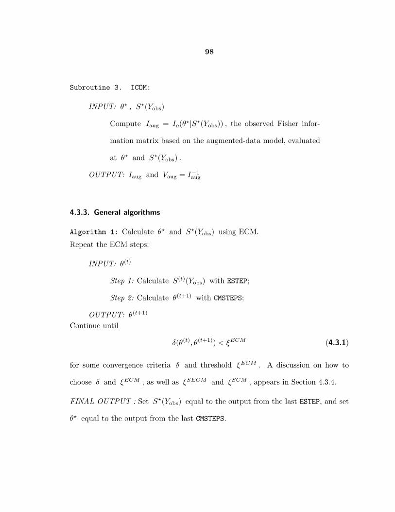
98

Subroutine 3. ICOM:

INPUT: θ⋆ , S⋆(Yobs)

Compute Iaug = Io(θ⋆|S⋆(Yobs)) , the observed Fisher infor-

mation matrix based on the augmented-data model, evaluated

at θ⋆ and S⋆(Yobs) .

OUTPUT: Iaug and Vaug = I−1aug

4.3.3. General algorithms

Algorithm 1: Calculate θ⋆ and S⋆(Yobs) using ECM.

Repeat the ECM steps:

INPUT: θ(t)

Step 1: Calculate S(t)(Yobs) with ESTEP;

Step 2: Calculate θ(t+1) with CMSTEPS;

OUTPUT: θ(t+1)

Continue until

δ(θ(t), θ(t+1)) < ξECM (4.3.1)

for some convergence criteria δ and threshold ξECM . A discussion on how to

choose δ and ξECM , as well as ξSECM and ξSCM , appears in Section 4.3.4.

FINAL OUTPUT : Set S⋆(Yobs) equal to the output from the last ESTEP, and set

θ⋆ equal to the output from the last CMSTEPS.

99

Algorithm 2: Calculate DMECM using SECM.

Let rij be the (i, j) th element of the d × d matrix DMECM and define θ(t)(i)

as

θ(t)(i) = (θ⋆1 , . . . , θ

⋆i−1, θ

(t)i , θ⋆

i+1, . . . , θ⋆d), i = 1, . . . , d. (4.3.2)

That is, θ(t)(i) is θ⋆ with the i th component active, i.e. replaced by the i th

component of θ(t) .

Repeat the SECM steps:

INPUT: θ⋆ and θ(t)

Repeat steps 1 and 2 for each i

Step 1: Calculate θ(t)(i) from (4.3.2), treat it as input for

Algorithm 1, and run one iteration of Algorithm 1 (that is,

one ESTEP and one CMSTEPS) to obtain θ(t+1)(i) ;

Step 2: Obtain the ratio

r(t)ij =

θ(t+1)j (i) − θ⋆

j

θ(t)i − θ⋆

i

for j = 1, . . . , d; (4.3.3)

OUTPUT: {r(t)ij , i, j = 1, . . . , d} .

FINAL OUTPUT: DMECM = {r⋆ij} , where r⋆

ij = r(tij)ij is such that

δ(r(tij)ij , r

(tij+1)ij ) < ξSECM (4.3.4)

for some suitable convergence threshold ξSECM .

100

Algorithm 3: Calculate DMCM using SCM.

For notational simplicity, the same notation is used for the elements of DMCM as

was used for those of DMECM .

Repeat the SCM (e.g. supplemented CM) steps:

INPUT: θ⋆, θ(t) , and S⋆(Yobs)

Repeat steps 1 and 2 for each i

Step 1: Calculate θ(t)(i) from (4.3.2) and run CMSTEPS once

using S⋆(Yobs) and θ(t)(i) as input to obtain θ(t+1)(i) ;

Step 2: Obtain the ratio r(t)ij as in (4.3.3);

OUTPUT: {r(t)ij , i, j = 1, . . . , d} .

FINAL OUTPUT: DMCM = {r⋆ij} where all the r⋆

ij = rtij

ij are such that (4.3.4)

is satisfied for some convergence threshold for SCM, ξSCM .

When implementing the PECM algorithm, Algorithm 3 can be replaced by

a simple evaluation of (4.2.3). For the more general ECM algorithm, it can be com-

putationally advantageous to replace Algorithm 3 with the analytical calculations

described in (1.6.7) and (1.6.8). Finally, the outputs of ICOM and Algorithms 2

and 3 (i.e. Vaug , DMECM , DMCM ) are put together to calculate ∆V using

(4.2.6), and then (4.2.5) is used to obtain the desired variance-covariance matrix

Vobs .

4.3.4. Notes on implementation

The convergence criterion δ(a, b) is a discrepancy measure between a and b .

Common choices are (i) δ(a, b) = maxi |ai − bi|, (ii) δ(a, b) = maxi |(ai − bi)/ai|

101

or maxi |(ai − bi)/(ai + bi)| , and (iii) δ(a, b) = ||a − b||, where || · || denotes the

standard Euclidean norm, and ai and bi are the components of a and b . The

first of these, (i), was used in the examples in Section 4.4 and is generally fine unless

the magnitudes of the components vary greatly, in which case (ii) is preferred. The

same holds for SECM and SCM except that a and b are scalars, in which case (i)

and (iii) are the same.

When ECM is run alone, the convergence threshold ξECM can be set to

obtain whatever level of precision is desired for θ⋆ . When SECM is used, how-

ever, ξECM must be quite small (compared to the magnitude of θ⋆ ) to insure

convergence of θ(t) as well as r(t)ij and thereby to insure satisfactory symmetry

in ∆V . Generally, ξSECM and ξSCM should be about equal to the square root

of ξECM , as discussed further in Section 4.5.1. Finally, note that Algorithms 2

and 3 assume that the ECM iterates were saved when Algorithm 1 was run. This

saves computational time, but requires extra storage. For some users, it may be

better to recompute the iterates than to save them. To do this, change the in-

put in Algorithms 2 and 3 to “INPUT: θ⋆ and θ(t−1) ” and add “Step 0: Run

one ECM iteration on θ(t−1) to obtain θ(t) .” Generally, it is not necessary to

start the SECM or SCM algorithms at θ(0) or to run them for as many steps as

ECM was run. Thus, saving all the iterates may not be economical, and it may be

computationally more efficient to recompute only the iterates that are needed.

102

4.4. Examples Illustrating the SECM Algorithm

4.4.1. Introduction to examples

In this section we present several examples that illustrate different aspects of SECM.

The first example is a simple bivariate normal used in Meng (1994) to illustrate

several surprising phenomena concerning the rates of convergence of EM, ECM, and

their variations. It shows how the basic building blocks of ECM are put together.

We also compare our simulation results to the theoretical results presented in Meng

(1994).

Our second example is a bivariate normal with stochastic censoring, often

applied in economics and known as the Type II Tobit model (e.g. Amemiya, 1984).

We demonstrate the easy implementation of SECM for this class of practically

useful models. We also show how inspecting the symmetry of the resulting variance-

covariance matrix led to the discovery of an error in the literature for computing

the E-step.

The third example illustrates a class of important applications of SECM –

computing the asymptotic variance-covariance matrix of maximum likelihood es-

timates fit to contingency tables in the presence of incomplete observations. The

algorithm essentially uses only the standard Iterative Proportional Fitting, or IPF

algorithm (e.g., Bishop, Feinberg and Holland, 1975) and a simple E-step that al-

locates the counts according to the estimated conditional cell probabilities.

Our last example is presented for numerical comparison with SEM results.

Meng and Rubin (1991a) uses this example to illustrate a variety of issues involved

103

in implementing EM and SEM. We repeat these for ECM and SECM, which allows

us to make direct comparisons with the results in Meng and Rubin (1991a).

4.4.2. A simple theoretical example

Suppose the augmented data consist of two observations from a bivariate normal

distribution

Yi =

(yi1

yi2

)iid∼ N

[(θ1θ2

),

(1 ρρ 1

)], i = 1, 2,

but we only observe z1 = y11 and z2 = y22 − y21 . Here ρ is known and we

are interested in the MLE θ⋆ of θ = (θ1, θ2) based on z1 ∼ N(θ, 1) and z2 ∼

N(θ2−θ1, 2(1−ρ)) . In this case the MLE is in closed form, θ⋆ = (z1, z1+z2) , with

variance-covariance matrix

(1 11 3 − 2ρ

)since z1 and z2 are independent. Thus,

this example allows us to compare empirical results with the theoretical values.

The E- and CM-steps follow simply from properties of the bivariate normal

distribution. Since ρ is known, the augmented-data sufficient statistics are simply

(y1, y2) , where yj = 12 (y1j + y2j) . Thus,

E :

{y(t)1 = E(y1|z1, z2, θ(t)) = z1

2+ 1

4(θ

(t)1 + θ

(t)2 − z2)

y(t)2 = E(y2|z1, z2, θ(t)) = 1

2 (θ(t)2 + ρ(z1 − θ

(t)1 )) + 1

4 (θ(t)1 + θ

(t)2 + z2),

CM1 : θ(t+ 1

2 )1 = y

(t)1 + ρ(θ

(t)2 − y

(t)2 ),

CM2 : θ(t+ 2

2 )2 = y

(t)2 + ρ(θ

(t+ 12 )

1 − y(t)1 ),

Notice that the E-step can easily be derived using the fact that y21 + y22 is inde-

pendent of y22 − y21 and that the latter is observed. Iterating these three steps

as in Algorithm 1 leads to θ⋆ . To implement SECM, we first run Algorithm 2 of

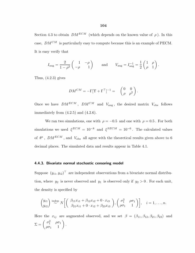
104

Section 4.3 to obtain DMECM (which depends on the known value of ρ ). In this

case, DMCM is particularly easy to compute because this is an example of PECM.

It is easy verify that

Iaug =2

1 − ρ2

(1 −ρ

−ρ 1

)and Vaug = I−1

aug =1

2

(1 ρρ 1

).

Thus, (4.2.3) gives

DMCM = −Γ[Υ + Γ⊤]−1 =

(0 0ρ ρ2

).

Once we have DMECM , DMCM and Vaug , the desired matrix Vobs follows

immediately from (4.2.5) and (4.2.6).

We ran two simulations, one with ρ = −0.5 and one with ρ = 0.5 . For both

simulations we used ξECM = 10−8 and ξSECM = 10−6 . The calculated values

of θ⋆ , DMECM , and Vobs all agree with the theoretical results given above to 6

decimal places. The simulated data and results appear in Table 4.1.

4.4.3. Bivariate normal stochastic censoring model

Suppose (yi1, yi2)⊤ are independent observations from a bivariate normal distribu-

tion, where y2 is never observed and y1 is observed only if y2 > 0 . For each unit,

the density is specified by

(yi1

yi2

)indep∼ N

[(β11xi1 + β12xi2 + 0 · xi3

β21xi1 + 0 · xi2 + β23xi3

),

(σ2

1 ρσ1

ρσ1 1

)], i = 1, . . . , n.

Here the xij are augmented observed, and we set β = (β11, β12, β21, β23) and

Σ =

(σ2

1 ρσ1

ρσ1 1

).

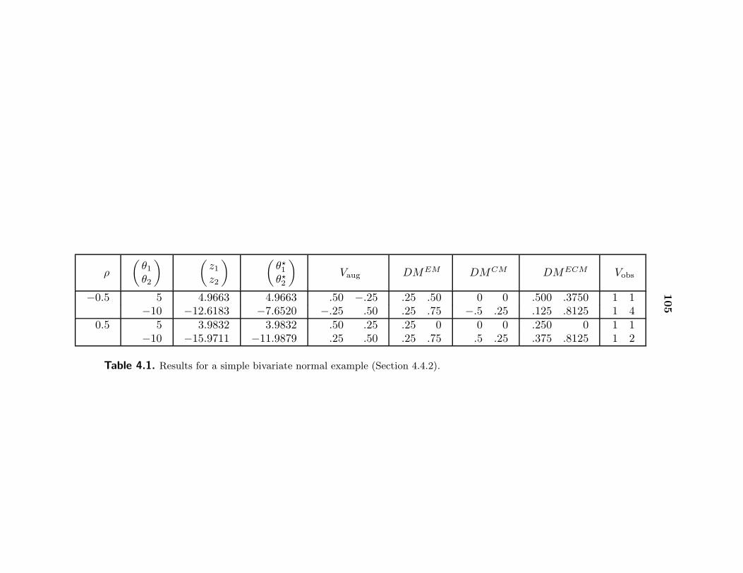
105

ρ

(θ1θ2

) (z1z2

) (θ⋆1

θ⋆2

)Vaug DMEM DMCM DMECM Vobs

−0.5 5 4.9663 4.9663 .50 −.25 .25 .50 0 0 .500 .3750 1 1−10 −12.6183 −7.6520 −.25 .50 .25 .75 −.5 .25 .125 .8125 1 4

0.5 5 3.9832 3.9832 .50 .25 .25 0 0 0 .250 0 1 1−10 −15.9711 −11.9879 .25 .50 .25 .75 .5 .25 .375 .8125 1 2

Table 4.1. Results for a simple bivariate normal example (Section 4.4.2).

106

This is an example of the so-called seemingly unrelated regression model

(Zellner, 1962), also known in economics as the Type II Tobit model (e.g., Amemiya,

1984). When the active covariates for yi1 and yi2 overlap but are not identical (in

our example, β13 = β22 = 0 ), even if all the y ’s are observed, the MLEs of β and

Σ are not in closed form. Consequently, implementing EM would require nested

iterations within the M-step. However, given β , the conditional MLE of Σ is

simply the sum of squares of the residuals divided by n . On the other hand, given

Σ , the conditional MLE for β can be easily obtained by weighted least squares.

ECM replaces the iterative M-step with these two CM-steps (detailed formulas are

given in Meng and Rubin, 1994b).

To compute the E-step, we need to find the conditional expectation of

(yi1, y2i1, yi2, y

2i2, yi1yi2) for i = 1, 2, . . . , n , given the observed data and the pa-

rameters. These calculations follow from the properties of the bivariate normal

distribution and are given explicitly in Little and Rubin (1987, p. 225). There is,

however, an error in that presentation. When yi2 > 0 , we also observe yi1 , and

must thus find E(yi2|yi1, yi2 > 0) and E(y2i2|yi1, yi2 > 0) , not E(yi2|yi2 > 0) and

E(y2i2|yi2 > 0) as presented there. This error will lead to incorrect results; in partic-

ular, it tends to underestimate the magnitude of ρ . For the data described below,

the true ρ = 0.5 , the MLE ρ⋆ = 0.482 , but the incorrect procedure gives 0.200. We

discovered this error only after we found that the resulting variance-covariance ma-

trix from SECM was clearly asymmetric, which demonstrates the power of SECM

as a tool for detecting errors in implementing ECM. To correct the E-step, we need

to substitute the following two expectations for the second and fifth equations given

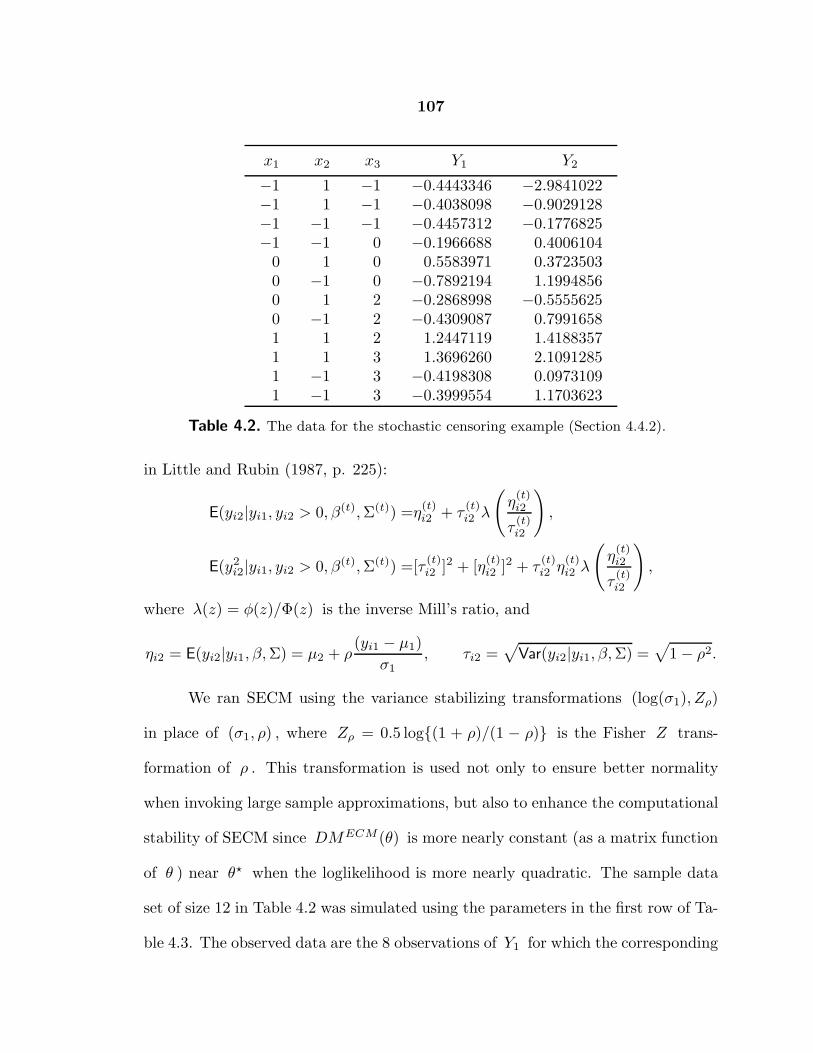
107

x1 x2 x3 Y1 Y2

−1 1 −1 −0.4443346 −2.9841022−1 1 −1 −0.4038098 −0.9029128−1 −1 −1 −0.4457312 −0.1776825−1 −1 0 −0.1966688 0.4006104

0 1 0 0.5583971 0.37235030 −1 0 −0.7892194 1.19948560 1 2 −0.2868998 −0.55556250 −1 2 −0.4309087 0.79916581 1 2 1.2447119 1.41883571 1 3 1.3696260 2.10912851 −1 3 −0.4198308 0.09731091 −1 3 −0.3999554 1.1703623

Table 4.2. The data for the stochastic censoring example (Section 4.4.2).

in Little and Rubin (1987, p. 225):

E(yi2|yi1, yi2 > 0, β(t),Σ(t)) =η(t)i2 + τ

(t)i2 λ

(η(t)i2

τ(t)i2

),

E(y2i2|yi1, yi2 > 0, β(t),Σ(t)) =[τ

(t)i2 ]2 + [η

(t)i2 ]2 + τ

(t)i2 η

(t)i2 λ

(η(t)i2

τ(t)i2

),

where λ(z) = φ(z)/Φ(z) is the inverse Mill’s ratio, and

ηi2 = E(yi2|yi1, β,Σ) = µ2 + ρ(yi1 − µ1)

σ1, τi2 =

√Var(yi2|yi1, β,Σ) =

√1 − ρ2.

We ran SECM using the variance stabilizing transformations (log(σ1), Zρ)

in place of (σ1, ρ) , where Zρ = 0.5 log{(1 + ρ)/(1 − ρ)} is the Fisher Z trans-

formation of ρ . This transformation is used not only to ensure better normality

when invoking large sample approximations, but also to enhance the computational

stability of SECM since DMECM (θ) is more nearly constant (as a matrix function

of θ ) near θ⋆ when the loglikelihood is more nearly quadratic. The sample data

set of size 12 in Table 4.2 was simulated using the parameters in the first row of Ta-

ble 4.3. The observed data are the 8 observations of Y1 for which the corresponding

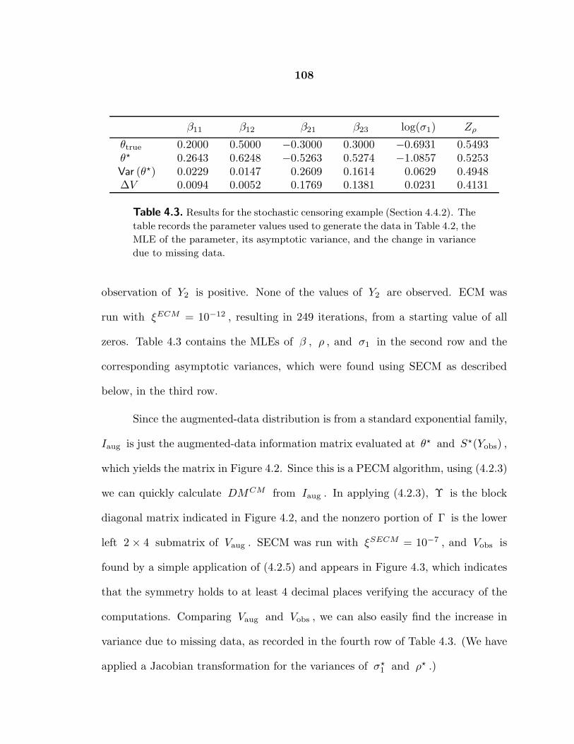
108

β11 β12 β21 β23 log(σ1) Zρ

θtrue 0.2000 0.5000 −0.3000 0.3000 −0.6931 0.5493θ⋆ 0.2643 0.6248 −0.5263 0.5274 −1.0857 0.5253Var (θ⋆) 0.0229 0.0147 0.2609 0.1614 0.0629 0.4948∆V 0.0094 0.0052 0.1769 0.1381 0.0231 0.4131

Table 4.3. Results for the stochastic censoring example (Section 4.4.2). The

table records the parameter values used to generate the data in Table 4.2, the

MLE of the parameter, its asymptotic variance, and the change in variance

due to missing data.

observation of Y2 is positive. None of the values of Y2 are observed. ECM was

run with ξECM = 10−12 , resulting in 249 iterations, from a starting value of all

zeros. Table 4.3 contains the MLEs of β , ρ , and σ1 in the second row and the

corresponding asymptotic variances, which were found using SECM as described

below, in the third row.

Since the augmented-data distribution is from a standard exponential family,

Iaug is just the augmented-data information matrix evaluated at θ⋆ and S⋆(Yobs) ,

which yields the matrix in Figure 4.2. Since this is a PECM algorithm, using (4.2.3)

we can quickly calculate DMCM from Iaug . In applying (4.2.3), Υ is the block

diagonal matrix indicated in Figure 4.2, and the nonzero portion of Γ is the lower

left 2 × 4 submatrix of Vaug . SECM was run with ξSECM = 10−7 , and Vobs is

found by a simple application of (4.2.5) and appears in Figure 4.3, which indicates

that the symmetry holds to at least 4 decimal places verifying the accuracy of the

computations. Comparing Vaug and Vobs , we can also easily find the increase in

variance due to missing data, as recorded in the fourth row of Table 4.3. (We have

applied a Jacobian transformation for the variances of σ⋆1 and ρ⋆ .)

109

Vaug =

β11 β12 β21 β23 log(σ1) Zρ

β11 0.013512 0.000000 0.001210 0.007259... −0.002169 −0.008234

β12 0.000000 0.009502 0.013557 0.000000... 0.000000 0.000000

β21 0.001210 0.013557 0.083980 0.003880... −0.000009 −0.002012

β23 0.007259 0.000000 0.003880 0.023278... −0.000051 −0.012073

· · · · · · · · · · · · · · · · · · · · ·

log(σ1) −0.002169 0.000000 −0.000009 −0.000051... 0.039834 0.016296

Zρ −0.008234 0.000000 −0.002012 −0.012073... 0.016296 0.081700

Figure 4.2. The augmented-data variance-covariance matrix for the stochastic censoring example (Sec-

tion 4.4.3). When implementing PECM, the block structure can be used to easily calculate DMCM .

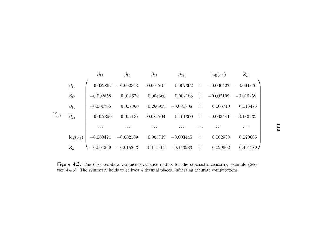
110

Vobs =

β11 β12 β21 β23 log(σ1) Zρ

β11 0.022862 −0.002858 −0.001767 0.007392... −0.000422 −0.004376

β12 −0.002858 0.014679 0.008360 0.002188... −0.002109 −0.015259

β21 −0.001765 0.008360 0.260939 −0.081708... 0.005719 0.115485

β23 0.007390 0.002187 −0.081704 0.161360... −0.003444 −0.143232

· · · · · · · · · · · · · · · · · · · · ·

log(σ1) −0.000421 −0.002109 0.005719 −0.003445... 0.062933 0.029605

Zρ −0.004369 −0.015253 0.115469 −0.143233... 0.029602 0.494789

Figure 4.3. The observed-data variance-covariance matrix for the stochastic censoring example (Sec-

tion 4.4.3). The symmetry holds to at least 4 decimal places, indicating accurate computations.

111

Survival (S)Clinic (C) Prenatal Care (P) Died Survived

(a) Completely Classified CasesA Less 3 176

More 4 293

B Less 17 197More 2 23 N (a) = 715 cases

(b) Partially Classified Cases? Less 10 150

More 5 90 N (b) = 255 cases

Table 4.4. A 2 × 2 × 2 contingency table with partially classified obser-

vations.

4.4.4. A 2× 2× 2 contingency table

Table 4.4(a) presents a 2 × 2 × 2 contingency table on infant survival (Bishop,

Feinberg, and Holland, 1975, Table 2.4-2). The supplementary data in Table 4.4(b)

was added by Little and Rubin (1987, p. 187) to form a partially classified table.

Suppose we wish to fit a log-linear model with no three-way interaction:

log(θijk) = u0 + (−1)i−1uP + (−1)j−1uC + (−1)k−1uS

+ (−1)i+juPC + (−1)j+kuCS + (−1)i+kuPS, (4.4.1)

where θijk is the cell probability for cell (i, j, k) for i, j, k = 1, 2 , with i cor-

responding to P , j to C and k to S . We will derive the MLE of U =

(u0, uP , . . . , uPS)⊤ and Vobs , the asymptotic variance-covariance matrix of U⋆ .

Meng and Rubin (1991b, 1993) describe an ECM algorithm with three CM-

steps for this problem. Specifically, since the loglikelihood is linear in the cell counts,

112

Y = {yijk} , the E-step simply involves imputing the missing data,

E : y(t)ijk = y

(a)ijk + y

(b)ik

θ(t)ijk∑

j θ(t)ijk

, (4.4.2)

where y(a)ijk are the cell counts in Table 4.4(a), and y

(b)ik are the marginal counts

classified only according to parental care and survival (see Table 3(b)). The CM-

steps make use of IPF. Given the current estimated cell probabilities {θ(t)ijk} , the

three CM-steps are

CM1 : θ(t+ 1

3 )

ijk = θ(t)ij(k)

yij+

N

CM2 : θ(t+ 2

3 )

ijk = θ(t+ 1

3 )

i(j)k

yi+k

N

CM3 : θ(t+ 3

3 )

ijk = θ(t+ 2

3 )

(i)jk

y+jk

N

where N is the total count, θij(k) = θijk/∑

k θijk is the conditional probability

of the third factor given the first two, and yij+ =∑

k yijk , etc. It is easy to

see that CM 1 maximizes L(θ|Y ) subject to θij(1) = θ(t)ij(1) for each i and j ,

so that the constraint function g1(θ) = {θij(1)} . Likewise g2(θ) = {θi(1)k} and

g3(θ) = {θ(1)jk} . It is clear that this is not a PECM algorithm.

We start ECM with θijk = 18 for each i , j , and k , which satisfies the

constraint of no three-way interaction, and cycle according to ECM : E → CM1 →

CM2 → CM3. At each iteration, U (t) can then be calculated by regression

U (t) = (X⊤X)−1X⊤ log θ(t), t = 1, 2, 3, . . . (4.4.3)

where the design matrix X is derived from (4.4.1) with elements either +1 or

−1 . Notice that we are defining two mappings, Mθ : θ(t) → θ(t+1) and MU :

U (t) → U (t+1) . The θ parameterization is more natural in the context of the E

113

and CM-steps. The U parameterization is more convenient in the context of the

log-linear model, and is a stable parameterization for the SECM calculations.

To compute Vobs on the U scale we need to derive DMECM , DMCM ,

and Vaug ≡ Var(U⋆|Y ⋆) , where Y ⋆ = E(Y |θ⋆, Yobs) . Implementing Algorithm 2

on the mapping induced by MU will yield DMECM . Since this is not a PECM

algorithm, we cannot use (4.2.3) to derive DMCM . Instead, SCM in Algorithm

3 is used. Replace Y (t) = {Y (t)ijk , i, j, k = 1, 2} with Y ⋆ in each CM-step and

use the CM algorithm iteration, CM1 → CM2 → CM3 in CMSTEPS; Algorithm 3

differentiates this mapping and produces DMCM . Finally, we compute Vaug via a

log-linear models package. Since all standard programs use the sufficient statistics

as their input, and Iaug is linear in the augmented-data sufficient statistics, fitting

(4.4.1) using Y ⋆ as the data will yield Vaug . For example, in ‘S’ (AT&T Bell

Laboratories) Vaug can be computed with

> model<-glm(formula= Y ⋆ ~ P + C + S + PC + PS + CS,

family = poisson(link = log))

> summary(model)$cov.unscaled

where P, C, S, etc. are vectors of +1 and −1 determined by (4.4.1) and are the

columns of the design matrix X . The parameter u0 in (4.4.1) is just a scale

parameter that insures that∑θijk = 1 and it should be ignored in the calculation

of Vobs as there are only six free parameters. Replace DMECM , DMCM , and

Vaug with the 6× 6 submatrices corresponding to the other six parameters before

computing Vobs using (4.2.5).

The results are presented in Table 4.5. The calculated matrix Vobs was

symmetric to nine places beyond the decimal, which is more accurate than expected

114

uP uS uC uPS uCS uPC

U⋆ † 0.406944871 −1.565681190 0.181533221 −0.044421642 −0.424777146 −0.661665499sd(U⋆) 0.117611832 0.092744286 0.135159680 0.117485008 0.132665503 0.058468375

0.013832543 −0.001820669 0.010260487 0.012248728 0.009021917 −0.001188741−0.001820668 0.008601503 0.003117087 −0.002317203 0.002471191 −0.000336477

Vobs 0.010260487 0.003117086 0.018268139 0.008670460 0.016175245 −0.0016023120.012248728 −0.002317204 0.008670459 0.013802727 0.009881752 0.0011450660.009021918 0.002471190 0.016175245 0.009881753 0.017600136 0.000532728

−0.001188741 −0.000336477 −0.001602312 0.001145066 0.000532728 0.003418551

† u⋆0 = −3.329440804

Table 4.5. The MLE U⋆ and Vobs for model (4.4.1) with data given in Table 4.4

.

115

Survival (S)Clinic (C) Prenatal Care (P) Died Survived

A Less [0.0016, 0.0115] [0.2244, 0.2876]More [0.0040, 0.0156] [0.3566, 0.4200]

B Less [0.0180, 0.0391] [0.2531, 0.3181]More [0.0013, 0.0090] [0.0205, 0.0457]

Table 4.6. 95% marginal confidence intervals for θ⋆ in model (4.4.1).

since the algorithm was run with ξECM = 10−16 , ξSECM = 10−8 , and ξSCM =

10−7 . The ECM algorithm required 70 iterations to converge.

The information in Table 4.5 can be used to construct confidence inter-

vals. For example, we can derive the Jacobian J of the transformation from

logit(θ) to U in order to calculate the observed Fisher information matrix for

logit(θ⋆) : Io(logit(θ⋆)|Yobs) = J⊤Io(U⋆|Yobs)J. Assuming approximate normality

on the logit(θ) scale, we can construct confidence intervals for each of logit(θijk) ,

and then transform to the θ scale. Table 4.6 is an illustration.

The calculations presented in the context of this example are in fact quite

general. Bishop, Feinberg, and Holland (1975) describes how either IPF or closed

form solutions can be used to fit any hierarchical log-linear model to contingency

tables with augmented data. This means that the CM-steps can easily be identified

for any such model. Since the E-step in (4.4.2) can easily be generalized to any

table with incomplete data, the SECM algorithm for fitting a log-linear model to

any table can easily be formulated. These calculations are described more fully by

van Dyk (1993).

116

Y1 8 6 11 22 14 17 18 24 19

Y2 59 58 56 53 50 45 43 42 39

Y1 23 26 40 4 4 5 6 8 10

Y2 38 30 27 - - - - - -

Table 4.7. The data used in the monotone missing-data example (Sec-

tion 4.4.5.

4.4.5. A bivariate normal example

The data given in Table 4.7 are assumed to follow a bivariate normal distribution

with parameters (µ1, µ2, σ1, σ2, ρ) . As in Meng and Rubin (1991a), we will use the

parameterization θ = (µ1, µ2, log σ1, log σ2, Zρ) . Notice that because of the mono-

tone pattern of missing values, there is no missing information for ϑ1 = (µ1, σ1) ,

and hence we can use either the standard ECM algorithm, or first estimate ϑ1

to get ϑ⋆1 using standard augmented-data estimates and then use ECM ∗ of Sec-

tion 4.2.4 to find ϑ⋆2 . To implement the standard ECM algorithm, we will use the

the two CM-steps

CM1 : ϑ(t+ 1

2 )1 = CM(ϑ1

∣∣ϑ(t)2 )

CM2 : ϑ(t+ 2

2 )2 = CM(ϑ2

∣∣ϑ(t+ 12 )

1 ), (4.4.4)

where ϑ2 = (µ1, log σ1, Zρ) , and the function CM(ξ|φ) takes on the value of ξ that

maximizes Q(θ|θ(t)) conditional on φ . To implement ECM ∗ , we will fix ϑ1 = ϑ⋆1

and use the algorithms in Section 4.3. We need only note that the input for ESTEP

is θ(t) = (ϑ⋆1, ϑ

(t)2 ) and CMSTEPS consists of the CM 2 -step given in (4.4.4). The

increase in variance due to the missing data, ∆V , can be calculated with (4.2.8)

117

where ∆V (ϑ⋆2|ϑ⋆

1) is given by (4.2.7). DMECM∗

and ∆V (ϑ⋆2|ϑ⋆

1) are given in

Table 4.8 for several values of ξECM and ξSECM .

It is interesting to compare ECM ∗ with EM. Since there is no missing in-

formation for ϑ1 , in this example EM produces ϑ⋆1 in one step. Consequently, the

E-steps from EM after one iteration and form ECM ∗ both condition on ϑ1 = ϑ⋆1

and will produce the same sufficient statistics, S(t)(Yobs) for the same value of ϑ(t)2 .

It is a simple fact of calculus in this example that CM(ϑ2|ϑ1 = ϑ∗1) = CM(ϑ2) .

The maximization step from EM and ECM ∗ will produce the same value of ϑ(t+1)2

for the same value of S(t)(Yobs) after one iteration. Therefore, the mapping induced

on ϑ2 by running ECM ∗ will be the same as the mapping induced on ϑ2 by run-

ning EM. Comparing DMECM∗

given in Table 4.8 with DM⋆ given in Meng

and Rubin (1991a) verifies this. There is a slight difference between the number of

iterations required because we used the convergence criterion (i) of Section 4.3.4

whereas they used (iii) .

Since EM and ECM ∗ induce the same mappings in this situation, SEM and

SECM ∗ are identical. SECM has a distinct advantage over SEM, however. When

there is no missing information for ϑ1 , the standard SEM algorithm fails because

some of the denominators of (4.3.3) are zero and therefore a special version similar

to SECM ∗ must be implemented (Meng and Rubin, 1991a). Since the CM algo-

rithm does not converge in one iteration even when there is no missing information,

the denominators are never zero, and thus the situation is less critical for SECM

and we may proceed with the standard algorithm. Table 4.9 records the results of

applying the standard SECM algorithm given in (4.4.4). As is evident from Ta-

118

Stopping ECM SECMCriteria Iterations Iterations for DMECM∗

∆V (ϑ⋆2|ϑ⋆

1)ECM;SECM for ϑ⋆

2 DMECM∗

2 3 2 0.333 0.042 −0.052 1.151285 0.138119 −0.23252110−4; 10−2 25 7 6 6 1.407 0.289 0.010 0.170981 0.025525 −0.024140

11 5 3 −0.648 0.017 0.470 −0.110795 −0.008875 0.0399722 11 14 0.333 0.040 −0.028 1.085282 0.166673 −0.093734

10−8; 10−4 44 19 17 16 1.444 0.299 0.019 0.167022 0.028514 −0.00982020 12 17 −0.642 0.015 0.325 −0.093318 −0.009753 0.0193792 20 23 0.333 0.050 −0.028 1.085838 0.167083 −0.093349

10−12; 10−6 63 29 26 26 1.444 0.299 0.019 0.167087 0.028555 −0.00977829 20 26 −0.642 0.015 0.325 −0.093344 −0.009777 0.019352

Table 4.8. Number of ECM ∗ and SECM ∗ iterations and convergent values of DMECM∗

and ∆V (ϑ⋆2|ϑ⋆

1)under three different convergence threshold in the monotone missing-data example (Section 4.4.5).

119

Stopping ECM SECMCriteria Iterations Iterations ∆V

ECM; SECM for θ⋆ for DMECM

3 2 3 2 2 -0.216878 -0.026844 0.509994 0.034717 0.18348610−4; 4 3 3 3 3 0.008955 0.008688 -0.006716 0.004098 -0.014324

47 6 2 5 2 2 0.343573 0.060970 0.331937 0.125992 -0.41075110−2 5 6 7 5 6 0.023331 0.012508 0.135287 0.032239 -0.035117

10 7 11 7 5 -0.009776 -0.011889 -0.088636 -0.015762 0.0434228 6 8 7 8 0.022126 -0.001376 -0.116788 -0.003779 0.031776

10−8; 23 19 8 18 20 0.000889 -0.001061 -0.003298 -0.001884 0.00052488 26 9 23 13 20 -0.019489 -0.002430 1.196050 0.165772 -0.125586

10−4 7 21 23 7 22 0.001040 -0.001843 0.162477 0.025473 -0.00901023 19 23 9 22 -0.000522 0.000661 -0.091476 -0.008647 0.019110

44 31 41 34 41 -0.000001 0.000076 -0.000046 0.000073 0.00004410−12; 35 32 29 31 32 0.000001 0.000000 -0.000003 -0.000001 0.000000

130 47 31 44 34 41 0.000027 -0.000094 1.085844 0.166995 -0.09339910−6 28 33 35 31 34 0.000003 -0.000001 0.167081 0.028554 -0.009779

35 31 35 28 34 -0.000002 0.000000 -0.093342 -0.009777 0.019352

Table 4.9. Number of ECM and SECM iterations and convergent values of ∆V under three different conver-

gence thresholds in the monotone missing-data example (Section 4.4.5).

120

ble 4.8, however, the standard SECM algorithm requires approximating the zero

elements in the rate matrix and is therefore less efficient and less stable. In partic-

ular, SECM is slower to converge, requires smaller values of ξECM and ξSECM to

obtain satisfactory symmetry, and requires the calculation of the DMECM matrix,

which can be of a much larger dimension than the DMECM∗

matrix. Nevertheless,

it is noteworthy that standard SECM does produce Vobs , whereas SEM must be

modified in this situation.

4.5. Diagnostics and Variations

4.5.1. Checking the symmetry of Vobs

One of the most valuable properties of SECM is that, like SEM, it has a built-in

diagnostic. Section 4.3 describes all the steps required by SECM. It is the last

step, the computation of ∆V , that helps us know if mistakes have been made

in any of these steps. The variance-covariance matrix, Vobs = Vaug + ∆V, and

thus ∆V , must be symmetric, but if any of θ⋆ , DMECM , DMCM , or Iaug

are not calculated correctly, it is practically certain that the resulting ∆V and

hence Vobs will be asymmetric. The example in Section 4.4.1 documents that

this diagnostic not only checks the computation of Vobs but also detects errors

in implementing the E and CM-steps. Convergence of the θ(t) sequence does not

insure that the convergent value is the MLE, θ⋆ . Many erroneous algorithms

converge. In fact, we had an instance in which our algorithm increased the likelihood

121

at each step and converged, but the resulting Vobs was asymmetric. In this case,

careful checking led to the discovery of some subtle errors in implementation. There

is no other diagnostic known to us that can automatically detect these errors, and

one perhaps would never find them without the detection power of this tool. If

Vobs is symmetric, however, we are virtually assured that both θ⋆ and Vobs are

correct because it seems practically impossible to make separate errors in SECM

that cancel appropriately.

Even when SECM is implemented correctly, the convergence threshold ξECM

needs to be quite small in order to obtain a Vobs matrix with satisfactory symmetry;

this implies an increase in the number of iterations required, especially when θ is

of high dimension. The more precisely we calculate θ⋆ , the more accurately we are

able to compute Vobs , because we are able to compute DMECM and DMCM more

accurately, as demonstrated by the example in Section 4.4.5. In general ξSECM

and ξSCM are chosen to be about equal to the square root of ξECM . They should

be chosen as small as possible, however, so that (4.3.4) is satisfied for some tij

for each i and j . In order to increase the accuracy of DMECM and DMCM ,

ξSECM and ξSCM may even be different for different components. When deciding

on convergence thresholds, a good rule of thumb is that Vobs will be symmetric to

about half as many digits as θ⋆ is precise; for example, roughly, when ξECM is

10−8 , we can expect 3 or 4 digits of accuracy in Vobs . The accuracy of Vobs can

always be judged by its symmetry, however, and gross asymmetry always indicates

either errors in implementation or numerical imprecision; also see Section 5 of Meng

and Rubin (1991a).

122

4.5.2. Computing Vobs when implementing AECM

The AECM algorithm described in Chapter 3 is a generalization of ECM in which

the data-augmentation and model-reduction schemes are allowed to vary from it-

eration to iteration. Although this can lead to much faster algorithms, the mathe-

matical formulation of the rate matrix is much more complicated than that of ECM

(see Section 3.3). Consequently, direct implementation of the supplemented AECM

algorithm would be quite involved. Sometimes, however, there is an easy solution.

In Algorithms 2 and 3, we evaluate the ratio rij using the ECM iterates in order

to calculate DMECM and DMCM . But there is nothing that requires the use of

the ECM iterates in these algorithms, just the ECM code, and we can actually use

any sequence θ(t) converging to θ⋆ . For the AECM algorithm there is generally

a corresponding ECM mapping (i.e., from the first cycle of each AECM iteration).

Such an ECM mapping may not be useful for computing θ⋆ because it may not

be space filling, but it can be used for the SECM algorithm which does not re-

quire the space-filling condition once θ⋆ is obtained. In the case of MCECM, we

can also obtain the ECM code by simply dropping all but the first E-step for each

space-filling sequence of CM-steps. With the ECM code in hand, we can use the

AECM iterates as input for the algorithms and compute Vobs just as described in

Section 4.3. That is, AECM can be used when we calculate θ⋆ in Algorithm 1,

but the ECM algorithm should be used in Algorithms 2 and 3 in which ESTEP will

consist of one E-step, and CMSTEPS will consists of a space-filling set of CM-steps. If

the AECM iterations were not saved, we can simply run the ECM algorithm when

123

implementing the supplemented algorithm to calculate Vobs . Generally, running

ECM in this round will not slow the convergence, since we only need to start at

initial values that are close to θ⋆ .

Chapter 5

Efficient Model Reduction:

Permuting CM Steps

5.1. Introduction

The AECM algorithm developed in Chapter 3 can increase the efficiency of the EM

algorithm via a more flexible data-augmentation scheme and simplifies its imple-

mentation by reducing the augmented-data model. Chapter 2 developed a method

of selecting an efficient data-augmentation scheme. In the current chapter, we will

examine the possibility of building more efficient algorithms by looking at a key

aspect of model reduction in the context of the ECM algorithm. Specifically, with

ECM, model reduction extends the EM algorithm by replacing the M-step with sev-

eral CM-steps. Because each of the CM-steps maximizes Q(θ|θ(t)) over a different

subspace of Θ , the “space-filling” condition is required to guarantee that the whole

parameter space Θ will be searched after we perform a set of CM-steps, but there

is no restriction on the order in which we choose to perform them. Moreover, the

order of the CM-steps can significantly affect the number of iterations required for

124

125

convergence. Taking an extreme example, when the ECM algorithm was used to

fit a log-linear model to a certain sparse contingency table with partially classified

counts, the ECM algorithm with one order of CM-steps required 27 times as many

iterations (i.e., CPU time) as another order. It is therefore of practical interest

to conduct an investigation of the impact of ordering on the computation time re-

quired by ECM, especially since the same computations are required to implement

one iteration of ECM regardless of ordering.

The purpose of this chapter is twofold. First, using the common contingency

table problem, we illustrate the impact of changing orderings on the actual number

of steps required for convergence. Second, we bring to light several remarkable and

sometimes troubling phenomena that arose in our investigation. We will see how

the standard theory for studying such algorithms and the seemingly related theory

of stochastic iterative algorithms lead to conclusions that are quite different from

what we see in practice. At a very practical level, we will show that the missing-

data structure seems to be ancillary to the relative efficiency of CM-step orderings

and that in some situations one of the standard convergence criteria can be very

misleading. These findings reinforce a lesson that is often forgotten — empirical

study is an irreplaceable criterion for realistic evaluation. It is somewhat remarkable

that this lesson repeats itself again and again in one study, where theory, intuition

and common wisdom all fail the empirical evaluation.

In order to evaluate the effect of permuting CM-steps, the global rate of

convergence for ECM is introduced and developed in Section 5.2. The difference

between theory and empirical findings is reported in Section 5.3, which discusses

126

reversing the order of CM-steps, and an investigation of general permutations is

presented in Section 5.4. Section 5.5 explores the sources of variation in iterations

required for convergence. In light of the theory of stochastic relaxation, Section 5.6

studies the question of whether it is a good strategy in practice to cycle through the

different permutations of CM-steps or to randomly select an order at each iteration.

Section 5.7 provides concluding remarks including several interesting practical issues

in selecting a convergence criterion.

5.2. The Rate of Convergence of ECM

5.2.1. The matrix rate

In Section 1.6 we presented the matrix and global rates of convergence for EM. In

the development of the SECM algorithm, the matrix rate was extended to ECM in

Section 4.2.2. In this section, we will extend the global rate to ECM. Like EM, the

ECM algorithm implicitly defines a mapping MECM : θ(t) → θ(t+1) = MECM (θ(t))

from the parameter space Θ to itself. Let θ⋆ be the limit of {θ(t) : t ≥ 0} . Suppose

that MECM (θ) is differentiable in a neighborhood of θ⋆ . Then a Taylor’s series

approximation yields

(θ(t+1) − θ⋆) ≈ (θ(t) − θ⋆)DMECM (θ⋆)

where

DMECM (θ) =

(∂MECM

j (θ)

∂θi

),

127

and DMECM (θ⋆) is nonzero when there is missing information (Dempster, Laird,

and Rubin, 1977; Meng and Rubin, 1991a, 1994a) or when there is more than one

CM-step. Thus, the ECM mapping is linear if we ignore the higher order terms in

the Taylor’s series expansion. This approximation becomes exact at convergence of

ECM, and thus DMECM (θ⋆) is called the (matrix) rate of convergence of ECM

(e.g., Meng, 1994). Since DMECM (θ) will always be evaluated at θ = θ⋆ , we will

suppress the dependency on θ when referring to the matrix rate of convergence.

5.2.2. The global rate

As with EM, in order to assess convergence, consider the ratio

rt =||θ(t) − θ⋆||

||θ(t−1) − θ⋆|| , t = 1, 2, . . . (5.2.1)

where || · || is the Euclidean norm. Algorithms which have smaller values of rt

tend to converge more quickly. It is trivial to show that

limt→∞

∣∣∣∣∣∣t

√||θ(t) − θ⋆|| −

[t∏

i=1

ri

] 1t

∣∣∣∣∣∣= 0. (5.2.2)

The lim sup of the term ρt = t√

||θ(t) − θ⋆|| is known as the root convergence

factor (denoted ρ ) and is equal to the spectral radius of DMECM (i.e., the largest

norm of the eigenvalues; Ortega and Rheinboldt, 1970, 10.1.4). Equation (5.2.2)

says that the geometric mean of the rt tends to the spectral radius of DMECM .

Thus, the spectral radius of DMECM controls the rate of convergence of the ECM

algorithm, and, in theory, algorithms with smaller spectral radii are preferred. For

computational purposes, we will use the empirical root convergence factor ρt =

[∏t

i=2 ri]1/(t−1) , where ri = ||θ(i) − θ(i−1)||/||θ(i−1) − θ(i−2)|| , i ≥ 2 .

128

It is worth noting that if DMECM has a spectral decomposition under sim-

ilarity transformations (as is always the case with the EM mapping; see Meng

and Rubin, 1994a), r = limt→∞ rt exists and is equal to the spectral radius of

DMECM . Thus, in the EM literature (as in Section 1.6) the convergent value of

(5.2.1) is used to assess the rate of convergence of the algorithm. This will not suffice

in the ECM case as limt→∞ rt may not exist and lim supt→∞ rt can be greater than

the spectral radius. This is illustrated in Figures 5.1 and 5.2 with a pure linear iter-

ation of a particular DMECM matrix. In the figures, θ is three dimensional and

the componentwise rate of convergence is defined as rt,i = (θ(t)i −θ⋆

i )/(θ(t−1)i −θ⋆

i ) ,

i = 1, 2, 3 (i.e., (5.2.1) applied to each component).

In practice, the quantity of real interest is the actual number of iterations

an algorithm requires for convergence. If ρt can be well approximated by ρ , the

spectral radius of DMECM , then the number of iterations required for convergence,

N, is related to ρ via

N ∝ −1

log(ρ), (5.2.3)

where the constant of proportionality depends only on the starting value and the

convergence criterion.

5.2.3. Factors effecting the global rate

In order to study ρ under different orderings of CM-steps, we need to investigate

how DMECM varies with these orderings. As discussed in Chapter 1, Meng (1994)

showed that

[I −DMECM ] = [I −DMEM ][I −DMCM ], (5.2.4)

129

Estimating the Rates of convergence

iteration

com

pone

ntw

ise

rate

0 20 40 60 80 100

-4-2

02

4

Overall Rate

iteration

over

all r

ate

0 200 400 600 800 10000.

500.

550.

600.

650.

700.

750.

80

Figure 5.1. Rates of convergence with a com-

plex dominant eigenvalue. The plot shows the

overall rate of convergence (5.2.1) as a func-

tion of the iteration (solid line). The dashed

lines are (5.2.1) applied to components of θ .

Figure 5.2. The empirical root convergence

factor for large t . The plot shows that the os-

cillation of (5.2.1) around ρ (the straight line)

does not dampen. Note that lim sup rt >ρ = 0.692 .

ρ =0.692

ρ =0.692

130

where I is the identity matrix, DMEM = I − IobsI−1aug, and

DMCM = P1 · · ·PS, with Ps = ∇s[∇⊤s I

−1aug∇s]

−1∇⊤s I

−1aug and ∇s = ∇gs(θ

⋆).

(5.2.5)

In the above expressions, DMEM and DMCM denote the matrix rate of conver-

gence of the EM and CM algorithms respectively. From (5.2.4) – (5.2.5), we see that

DMECM depends on the data augmentation through DMEM and on the model

reduction scheme (in particular, the order of CM-steps) through DMCM where

the product of Ps ’s is calculated in the order that the CM-steps are performed.

There is another way of expressing DMCM that turns out to be theoretically

convenient:

DMCM = I12aug {A1 · · ·AS} I−

12

aug , (5.2.6)

where

As = ξs[ξ⊤s ξs]

−1ξ⊤s with ξs = I− 1

2aug∇s.

In other words, DMCM can be written as the product of symmetric (projection)

matrices.

5.3. Reversing the Order of CM-Steps

5.3.1. Theoretical results

Consider the two ECM algorithms, ECM (1,...,S) with steps ordered

E → CM1 → · · · → CMS ,

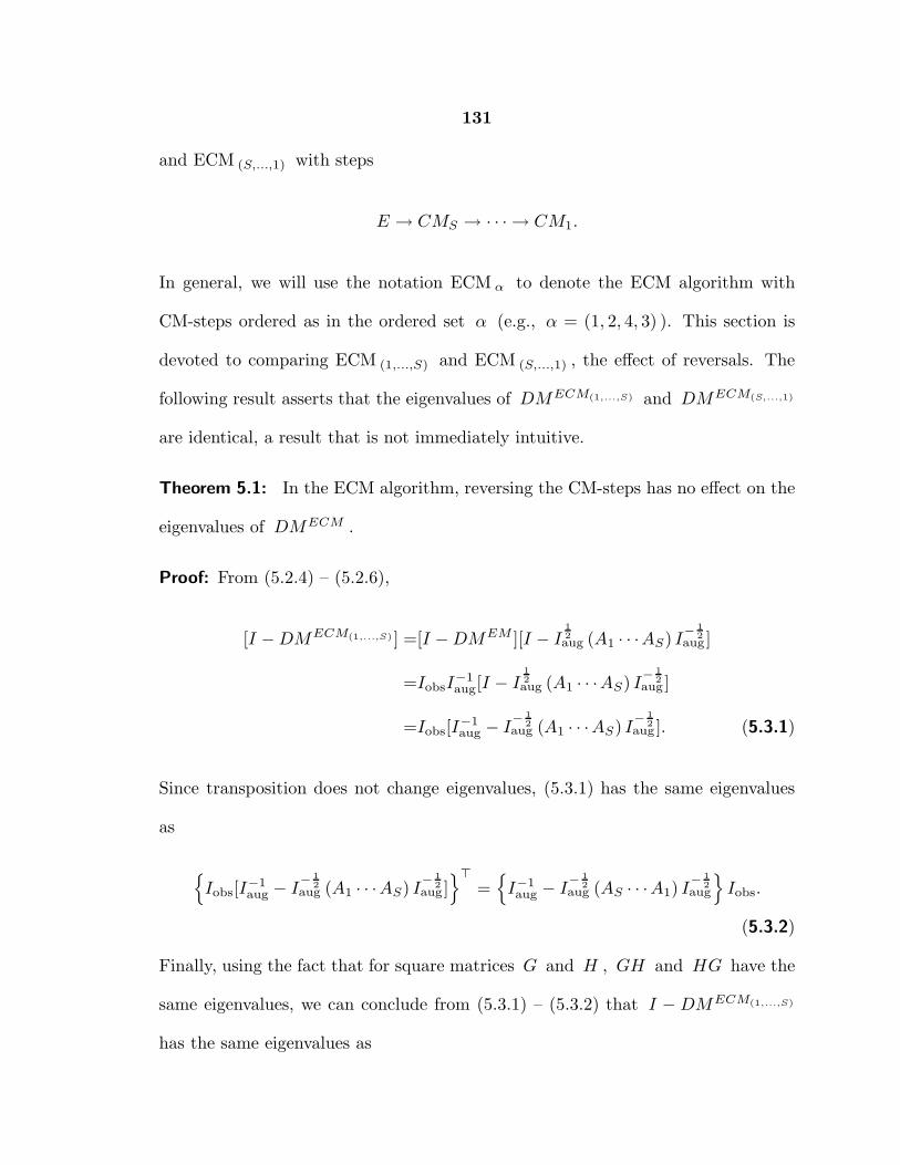
131

and ECM (S,...,1) with steps

E → CMS → · · · → CM1.

In general, we will use the notation ECM α to denote the ECM algorithm with

CM-steps ordered as in the ordered set α (e.g., α = (1, 2, 4, 3) ). This section is

devoted to comparing ECM (1,...,S) and ECM (S,...,1) , the effect of reversals. The

following result asserts that the eigenvalues of DMECM(1,...,S) and DMECM(S,...,1)

are identical, a result that is not immediately intuitive.

Theorem 5.1: In the ECM algorithm, reversing the CM-steps has no effect on the

eigenvalues of DMECM .

Proof: From (5.2.4) – (5.2.6),

[I −DMECM(1,...,S) ] =[I −DMEM ][I − I12aug (A1 · · ·AS) I

− 12

aug ]

=IobsI−1aug[I − I

12aug (A1 · · ·AS) I

− 12

aug ]

=Iobs[I−1aug − I

− 12

aug (A1 · · ·AS) I− 1

2aug ]. (5.3.1)

Since transposition does not change eigenvalues, (5.3.1) has the same eigenvalues

as

{Iobs[I

−1aug − I

− 12

aug (A1 · · ·AS) I− 1

2aug ]

}⊤

={I−1aug − I

− 12

aug (AS · · ·A1) I− 1

2aug

}Iobs.

(5.3.2)

Finally, using the fact that for square matrices G and H , GH and HG have the

same eigenvalues, we can conclude from (5.3.1) – (5.3.2) that I − DMECM(1,...,S)

has the same eigenvalues as

132

Iobs[I−1aug − I

− 12

aug (AS · · ·A1) I− 1

2aug ] = [I −DMEM ][I −DMCM(S,...,1) ]

= I −DMECM(S,...,1) .

From the discussion in Section 5.2, Theorem 5.1 tells us that reversing CM-

steps within the ECM algorithm does not effect the root convergence factor of the

algorithm. We must recall, however, that although ECM tends to be linear near

θ⋆ , little is known about its behavior away from θ⋆ . Moreover, the empirical root

convergence factor, ρt , is only asymptotically (with respect to t ) equal to the

spectral radius of DMECM . So even if the algorithm is linear, it may take many

iterations before ρt converges to the spectral radius.

5.3.2. Empirical results

To judge the applicability of Theorem 5.1, a simulation was performed. The ECM

algorithm was used to fit a log-linear model to data from a partially classified

2×2×2 contingency table (see Sections 3.5.2 and 4.4.4). This ECM algorithm has

three CM-steps, which correspond to the three steps of iterative proportional fitting

(IPF, Bishop, Feinberg, and Holland, 1975); the details are given in Section 4.4.4.

For each simulation 2000 data sets of size n were generated, of which nc were

completely classified and ni were classified only according to margin i ( i = 1, 2, 3 ).

Three simulations were run and the sample sizes for each appear in Table 5.1. Each

data set was generated from the no three-way interaction model

133

Sim. n nc n1 n2 n3

1 100 25 25 25 252 1000 100 300 300 3003 100 40 20 20 20

Table 5.1. Sample sizes for simulations 1-3. This table records the total

number of observations n , the number of observations that are completely

classified nc , and the number ni which were classified only according to

margin i .

Cyclic Permutations

Reversals of ECM (123) ECM (231) ECM (312)

CM Steps ECM (321) ECM (132) ECM (213)

Table 5.2. The ECM algorithms run in the simulations.

log(θijk) = u0 + (−1)i−1u1 + (−1)j−1u2 + (−1)k−1u3

+ (−1)i+ju12 + (−1)j+ku23 + (−1)i+ku13, (5.3.3)

where θijk is the cell probability for cell (i, j, k) . As an attempt to mimic the

variability in parameters governing real data sets, the log-linear parameters were

randomly selected for each data set from ul ∼ N(0, 1) , and ulm ∼ N(0, 0.25) , in-

dependently for l,m = 1, 2, 3 , and u0 was then chosen so that the cell probabilities

sum to one.

For each data set the model in (5.3.3) was fit using a starting value of

θ(0)ijk = 1

8 , which is frequently used in practice, with each of the six ECM algo-

rithms resulting from the six possible orderings of the CM-steps. Suppose Nij (i =

1, 2; j = 1, 2, 3) are the number of steps required for convergence of the six algo-

134

rithms where N1j correspond to three algorithms with different asymptotic rates

of convergence (c.f., columns of Table 5.2), and Ni1 correspond to the algorithms

with the CM-steps reversed (c.f., rows of Table 5.2). Consider the quantity,

R2 =12

∑i(N1j −N2j)

2

∑ij(Nij − N··)2

, (5.3.4)

which is the proportion of the total variation among the Nij that can be accounted

for by reversing the CM-steps. If Theorem 5.1 also implies that reversing the order

of CM-steps does not effect the actual number of steps required for convergence, R2

should be near zero. Figure 5.3 shows that simulated values of R2 from the three

simulations are actually skewed towards one (computed when the denominator of

(5.3.4) was greater than zero). Thus, step reversals seem to be more important than

Theorem 5.1 implies.

To explore this further, Figure 5.4 shows estimated densities for the possible

percent increase in efficiency due to (a) step reversals (dotted line:

1 − min(N1j, N2j)/max(N1j, N2j) ) and (b) general permutations (solid line: 1 −

mini,j(Nij)/maxi,j(Nij) ). Notice that although the effect of general step permuta-

tions is slightly greater than that of simple step reversals, the step reversals account

for the majority of the variation. This implies that when we consider the effect of

permutation of CM-steps on CPU time, we must consider all S! possible orderings

(as will be discussed in the following section). More than this, however, we must

be somewhat skeptical of analysis of convergence properties of EM-type algorithms

based solely on the spectral radius of the mapping matrix. Such analysis is much

better defined mathematically and more widespread in the literature than attempts

to look at the actual CPU time required for convergence, but may not answer

135

0.0 0.2 0.4 0.6 0.8 1.0

01

23

45

6Histogram of R squared

R2

% ti

mes

10

Maximum effect of Steps Reversals and Permutations

0.0 0.2 0.4 0.6 0.8 1.0

02

46

810

1214

percent increase in efficiency

Figure 5.3. A histogram of the 6000

values of R2 observed in the three sim-

ulations described in Table 5.1. Notice

that R2 tends to be large which sheds

doubt on the applicability of Theorem 1

to the number of steps required for con-

vergence.

Figure 5.4. The figure shows the den-

sity of percent decrease in iterations re-

quired due to (a) step reversals: [ 1 −min(N1j , N2j)/max(N1j , N2j) ] (dot-

ted line); and (b) general permutation:

[ 1−min(Nij)/max(Nij) ] (solid line).

questions that users actually face. (An even more relevant comparison in practice

should take into account the users’ effort for implementing different algorithms, an

issue that fortunately need not be considered here because implementing a different

ordering does not increase users’ effort). For completeness, in the next section, we

will present several results which bound the effect of permuting CM-steps on the

spectral radius, but the rest of the chapter will focus on on the actual CPU time,

or equivalently when making comparisons, the actual number of iterations.

136

5.4. General Permutations of CM-steps

5.4.1. Theoretical results

For an ECM algorithm with S CM-steps, there are S! possible orders. In this

section we will explore how much difference there is between these S! algorithms

with regard to CPU time. Again, we will begin our discussion with a look at the

root convergence factor and compare this with results from the simulation presented

in Section 5.3.

Theorem 5.2 will help us to put a bound on the effect of permuting CM-steps

on the spectral radius of DMECM in the three CM-step problem.

Theorem 5.2: For the general three CM-step ECM algorithm, the determinant of

I −DMECM is invariant under permutations of CM-steps.

Proof: First we observe that in the three step CM algorithm, the eigenvalues of

DMCM do not depend on the order of CM-steps. To see this, note (i) CM is

a special case of ECM with Iobs = Iaug , so the observation holds under CM-

step reversals (Theorem 5.1); (ii) it is clear from (5.2.6) that the observation holds

under cyclic permutations (for ECM the eigenvalues will generally change with

cyclic permutations of CM-steps because of the E-step). Together (i) and (ii) give

all possible permutations in the three step algorithm. From this observation it is

clear that |I −DMCM | is constant over permutations of CM-steps. Finally, note

137

that from (5.2.4), we have

|I −DMECM | = |Iobs| |I−1aug| |I −DMCM | (5.4.1)

The result is now clear since none of the quantities on the right are effected by

permutation of CM-steps.

For the general ECM algorithm, Theorem 5.2 holds only when S = 3 . For

the important special case of PECM, however, the result holds for any S .

Theorem 5.3: For the PECM algorithm (see for example Section 1.3),

|I −DMCM | =|Iaug|∏Si=1 |Υi|

and |I −DMECM | =|Iobs|∏Si=1 |Υi|

,

where Υi are the submatrices of the block diagonal matrix Υ (4.2.3). Both are

invariant under permutations of CM-steps.

Proof: From (4.2.3), we can write

[I −DMCM ] = [Υ + Γ⊤ + Γ][Υ + Γ⊤]−1 = Iaug[Υ + Γ⊤]−1.

Since [Υ + Γ⊤] is a block triangular matrix, with diagonal submatrices Υi , its

determinant is∏S

i=1 |Υi| , which gives the result for |I −DMCM | . Again, (5.4.1)

easily extends this to |I −DMECM | .

The following corollary relates Theorems 5.2 and 5.3 to the spectral radius of

DMECM .

Corollary: Let ρα ≤ ρβ be the spectral radii of DMECMα and DMECMβ respec-

tively, where ECM α and ECM β are either both PECM or both three step ECM

138

algorithms, and in either case, both algorithms are identical except for the order of

the CM-steps. Suppose

|I −DMECMβ | ≤ 1 − ρβ, (5.4.2)

then

ρβ ≥ ρα ≥ 1 − d√

1 − ρβ, (5.4.3)

where d is the dimensionality of θ .

Proof: Let 0 ≤ ||λα1|| ≤ · · · ≤ ||λαd|| ≡ ρα ≤ 1 be the ordered eigenvalue norms

(in complex space) of DMECMα ( ρα ≤ 1 whenever ECM α converges). Using the

fact that the determinant is the product of the eigenvalues, we have

(1 − ρα)d ≤d∏

i=1

||1 − λαi|| = |I −DMECMα | = |I −DMECMβ | ≤ 1 − ρβ,

where the first inequality follows from (1 − ρα) ≤ ||1 − λαi|| for i ≤ d .

Condition (5.4.2) is satisfied whenever all the eigenvalues of DMECMβ are

real and positive, a condition that holds for any EM algorithm. Unlike DMEM ,

however, it is possible for DMECM to have imaginary or negative eigenvalues.

But when this happens, our simulations show that the imaginary part of complex

eigenvalues or negative eigenvalues tends to be small in magnitude. We thus expect

that condition (5.4.2) can eventually be removed or proved to be true under simpler

conditions.

Although the bound in the corollary is very crude, it is nontrivial even for

quite large values of d (e.g., d ≥ 20 ). To see this we use (5.2.3) to put the corollary

in terms of the number of iterations required by the fastest and slowest algorithms

139

that result form permuting CM-steps. Specifically, suppose Nmax and Nmin are

the number of iterations required by the slowest and fastest algorithms respectively,

then

Nmin

Nmax≥ log(ρmax)

log(1 − d√

1 − ρmax), (5.4.4)

where ρmax is the root convergence factor of the slowest algorithm. A plot of the

right side of (5.4.4) for several values of d appears in Figure 5.5. This represents

the maximum improvement that we could see by permuting CM-steps as a function

of the slowest rate of convergence. Notice that the slower the algorithm (large ρ )

the more improvement we can hope for, which is consistent with our intuition. We

see that the crude bound provided by the corollary eliminates a nontrivial part of

the impossible values of Nmin/Nmax (i.e, the area below the curves in Figure 5.5).

5.4.2. Empirical Results

Recalling that (5.4.4) is based on the theoretical approximation (5.2.3), we again

turn our attention to the simulations described in Section 5.3 regarding the actual

number of steps required. The simulations use a three CM-step ECM algorithm and

falls under Theorem 5.2. The six possible ECM algorithms were run on each of the

data sets. The quantity Nmin/Nmax was calculated along with the empirical root

convergence factor at convergence of the slowest algorithm, ρt . Figure 5.6 shows a

plot of these for the three simulations along with results from a fourth simulation

run with n = 200 , nc = 140 , and ni = 20 for each i , which was added to include

smaller values of ρ (less missing information). The solid line is the right side of

(5.4.4) with d = 6 . Given that we have seen substantial discrepancy between

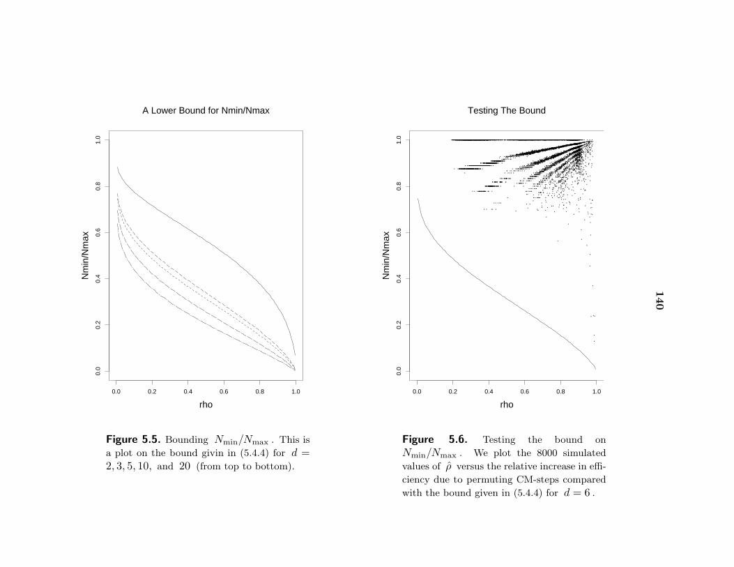
140

A Lower Bound for Nmin/Nmax

0.0 0.2 0.4 0.6 0.8 1.0

0.0

0.2

0.4

0.6

0.8

1.0

rho

Nm

in/N

max

Testing The Bound

0.0 0.2 0.4 0.6 0.8 1.00.

00.

20.

40.

60.

81.

0rho

Nm

in/N

max

.

.

.

.

.

.

.

.

.

.

.

.

..

.

.

.

..

.

.

. ..

..

.

. .

..

.

..

.

.

.

.

..

.

.

.

..

.

.. . .

. .

.. ..

.

. .

.

.

.

.

.

..

.

.

.

..

.

.. . .

.

.

.

.

.

..

.

.

..

. .

..

.

. .

.

..

..

..

.

. .. .

.

.

.

..

.

..

.

.

.

..

.

..

..

.. .

.

.

.

. .

..

.. .

.

.

...

.

. ..

.

.

.

.

.

.

..

...

..

.

.

.

. .

... ..

.

..

.

.

. ...

.

.

.

. . .

.

.

.

.

.

.

.

..

.

..

.

..

.

.

..

. .

.

.

.

.

.

.

.

..

..

..

.

.

...

.

.

..

.

.

...

..

..

..

. ..

...

..

.

.

..

.

.

.

..

..

..

.

.

.

.

.

..

.

. .

.

.

..

.

..

.

...

.

.

.

.

.

..

.

.

.

.

. .

..

.

. ..

.

.

...

.

.

..

..

.

. .

..

.

.

. .

.

.

..

.

.

.

.

.

.

.

.

.

.. ..

.

.

..

..

.

..

..

.

..

. ..

.

.

.

.

.

.

..

.

...

.

..

.

.

.. .

.

.

..

.

.

.

.

.

.

.

.. .

.

.

..

.

.

.

....

...

.

..

.

.

..

.

.

.

.

...

.

..

.

..

..

.

.

....

.

.

.

.

.

.

...

.

...

.

.

. .

.

...

..

.

.

.. .

.

.

.

.

.

.

.

..

.

.. ..

.

.

.

....

.

..

..

.

.

...

.

.. .

.

.

.

.

. .

.

.

.

.

.

.

.

.

.. ..

..

.

.

.

.

...

..

.

.

.

.

.

...

.

.

.

..

.

.

.

.

.

..

.

..

.

..

.....

...

.

.

..

..

.

.

..

.

..

.

. ...

.

.

.

.

.

.

.

.

.

.

.

.

.. .

.

..

..

... ..

.

.

.

.

.

..

.

.

. .

..

.

.

.

.

.

.

.

..

..

..

..

.

.

.

.

..

. ..

.

..

...

.

..

.

. .. ...

.

....

.

..

.

..

.

.

.

.

.

.

..

.

..

.

.

..

..

.

.

.

..

..

.

..

.

.

.

..

...

.

.

..

.. .

.

.

.

.

.

. .

..

..

. ..

.

. ..

.

.

.

.

.

.. .

.

.

.

.

...

.

.

.

.

..

.

.

..

. .

.

. .

... .

.

.

.

..

.

.

.

.

.

.

.

.

.

...

.

.

.

..

.

..

.

..

.

.

.

.

..

.

.

..

..

.

.

.

. .

.

. ..

.

.

.

.

.

.

.

.

.

.

..

.

.

.

. . .

.

..

.

.

..

.

..

.

.

. .

.

. .

.

.. .

.

. .

...

.

..

..

.

.

.

..

.

.

.

.

.

..

.

. .

.

..

. ..

.

.

.

.

.

.. .

.

.

.

.

..

.

.

.

....

.

. ..

.

.

..

.

..

..

.

.

.

.

.

..

. ..

.

.

.

.

. . .

...

.

.

.

.

.

..

.

.

.

..

.

..

.

.

..

..

...

.

.

.

...

..

.. .

.

.

..

. .

...

.

.

... .

...

....

.

..

..

.

.

..

.

..

..

.

..

..

..

..

..

.. ..

...

.

.

..

.

.

..

..

.

...

.

.

..

.

. ..

.

.

.

..

..

...

.

. .

.

.

.

.

..

.

.

.

.

.

..

..

.

..

.

..

.

. ..

.

.

. ..

...

.

. ..

.

.

.

.

..

.

.

.

.

..

.

. .

. .

.

.

.

.

.

.

..

.

..

..

..

.

.

.

..

.

.

.

. .

.

..

...

.

.

.

.

.

..

.

.

...

.

..

..

..

.

.. ..

.

..

..

.

.

.

.

.

...

.

.

.

..

.

..

.

.

.

.

..

..

.

.

..

..

.

..

.

..

..

.

.

.

.

.

.

.

.

.

.

.

.

.

.

. .

..

.

.

.. . .

..

.

...

.

..

..

..

..

.

.

..

..

.

.

...

.

.

...

.

.

.

.

.

..

.

.

..

.

..

.

...

. ..

. .. ...

...

.

.

..

.

.

.

.

..

.

.

.

.. .. .. .

.

.

.

... .

.

.

.

..

. ..

.

..

..

.

.

.

.

..

..

.

.

.

.

.

.

.

.

..

. .

.

.

. .

...

..

.

.. ..

.

.

.

.. .

.

.

.

.

..

.

. .

.

.

.

.

.

.

..

.

.

.

..

.

. ..

.

..

..

.

.

. .

.

.

.

....

.

.

....

..

.

..

. ....

.

.

.

.

. .

.

. .

.

.

.

.

.

. .

.

.

.

.

. . .

..

.

.

..

..

..

.

.

.

.

.

.

... . .

.... .

.

...

.

.

.

.

.

.

.

.

..

..

.

.

.

. .

..

. ..

. .

..

.

.

..

.

..

.

..

..

. ..

.

.

..

.

.

.

.

.

.

.

.

.

. . .

..

..

...

.

.

... ..

.. .

.

.

..

.

.

.

.

..

.

.

.

. ..

.

..

.

.

.

.

.

.

..

.

..

.

.

.

.

...

..

.

..

..

.

.

.

.

.

.

.

.

..

.

.

.

.

.

.

..

.

.

.

. .

..

..

..

.

.

.. .

.

.

..

.

..

. ...

..

.

..

. .

.

.

.

.

.

.

....

.

. .

.

.

.

..

.

..

.. ..

.

.

.

.

. ..

.

..

.

.

..

..

.

.

.

..

..

.

.

.

.

.

..

..

.

.

.. .

.

... ..

.

.

..

.

..

.. ...

.

.

..

.

.

.

.

.

.

..

.

...

.

.

.

.

.

. ..

.

.

.

.

.

..

..

.

...

..

.. .

.

..

.

.

..

..

.

. .

..

. .. .

.. .

.

. .

.

.

....

..

.

.

...

.

..

.

.

.

.

.

.

.

.

.

.

.

.

..

.

.

.

....

.

.

..

.

...

.

.

.

.

.

. .

...

.

.

...

.. .

.

.

.

..

.

.

.

.

..

..

..

..

.

.

.

..

.

.

..

.

.

.

.

.

.

..

..

.

.

..

.

.

.

.. .

.

.

...

.

..

.

.

.

. .

....

.

.

..

.

.

.

. .

...

.

.

.

.

.

.. .

.

.

. .

.

.

. .

.

.

. . .

.

..

..

.

..

..

..

.

.

.

..

.

...

.

.

..

.

.

. ..

.

..

.

.. .

.

.

..

..

..

...

.

.

..

.

.

.

.

..

..

.. .... .

.......

.

.

.

...

....

. ..

.

.....

..

.

......

.

.

.

. ..

....

...

...

. ...

..

.

..

. ...

.

.

..

.

....

.

. .

.

.....

.

.

.....

..

.

..

.....

.

.

..

.

.

. .

.

..

.

. ..

. .

.

.... ..

.

...

..

.

.

. ....

.

.

.

....

..... ..

..

.

.

.

. ..

...

..

....

..

.

.

.. ....

...

...

.

...

...

.

.

... ..

...... ...

.

.

.....

.

..

.

.

.

.

..

. ....

.

....

.. .

.

.

....

..

.

. ..

..

......

.

.

..

... ...

......

.. .

.

..

..

.

.

..

.....

.

. .

.

...

... .

.

. ...

...

.

.

.

...

....

..

.. ...

.

..

...

..

.

.

.

...

.

.

..

...

....

.. ...

.

..

.. ..

....

...

..

.

.

.

.

. ... ... ..

.

..

..

. ..

.

.

..

... .

...

. ... .....

..

.

. ..

.. ....

..

.

.

..

.

...

.. ..

..

...

.

.. .

..

.

.

..

.... ......

.

..

.. ....

.

...

.. .

. ... ..

.

.

.

....

.

.

... .

.

..

..

.

..

..

.

.

....

.

. ...

.

.

.

...

......

.... ..

.

.

..

.

. ....

.

..

.

.. ...

.

. .

...

...

..

..

. .

.. .

...

.. . ..

.. . .

.

.

........

..

...... .. ..

.

.

.

.

..

..

.

..

..

.

.....

.

.. .

.

.

...

...

....

..

..

.

... .

.

.

.

... .

..

. ..

..

.

.

.

.

.

.

..

.

...

.

.. ..

.. ..

..

.

..

... ......

.

.

......

. . ...

.

.

.

......

....

...

.....

... ... ...

.

..

..

.. .

.

. ..

.

.

.

. .......

. ....

.

.

...

..

.

.

..

. .

.

..

.

.

. .

.

.. .

.

.

.. .. .

...

.

..

.

..

.

.. ..

.. . ..... .

...

.

.

.

..

.

...

.

.

...

. ..

..

.

.

..

. ...

.

.

...

.

.

..

.

.

..

... .

......

.

.

.

..

..

.

.

. ..

.

.

.... .

.

... .

..

..

.

.

. .

..

.

.

.

.

.

..

.....

...

.

.

. . ...

.

..

.... .

.

..

...

.

.

. ..

...

.

...

.

..

...

....

.

.

.. .

.

..

.

.

. ....

.. .

.....

..

...

.

..

. .

.

...

..

.......

.

..

.

.

. .

. ..

.

.

.

..

..

.... .

. .. .

..

.

.

..

.

..

...

.

.

...

..

.

...

......... . .

.....

..

...

..

.

..

...

... .

.

.. ..

.

...

.....

..

....

. .. ...

.

.

..

.

.

.

.

..

.

.

.

...

.

...

..

.

. .. .

...

..

. .

.

.. ...

.. .

.....

.

. ..

...

..

.

..

.

... .. .

...

.

. ..

.

.

.. .... . ..

.. ..

..

....... ..

..

. ..

.

.

...

..

..

.

. ..

.

...

.

..

.....

..

..

... .

..

.

.......

.

...

.

.. .

....

..

. ... .

. ..

.

...

.

..

.

..

. ..

....

.

. ...

...

..

...

.

. .. ..

.

.

.

.. .....

. .

.

....

.

...

.

.

.

.

.

..

...

...

.

. .

..

.

..

. .

..

..

..

.

....

...

.

. .

.

...

.

.

.

.

...

.

..

...

.

...

..

... ..

. .

.. .

.. .

....

.

. .....

.

.

...

....

. ...

..

.. ..

.

.

. ..

.

.....

.

...

. ....

. ..

.

.

..

..

..

...

.

.

.

. ..

.

. ....

...

.

. .

.

.

...

...

.

.

.

...

....

.

..

..

.. ...

.

..

..

.

.

.

...

.

.. ..

....

.

.

..

.. .. ... ..

.

..

.

....

.

...

..

.

.....

.

. .

.

...

.... .... .

. ..

..

.

..

.. .

...

.

.

.

.

...

..

.

.

..

.

..

.

.

.

.....

... ....

.

... ..

.

....

.

.

.

...

.

.

... ..

...

. ....

...

.

.

.

.

..

...

..

.

...

..

..

.

...

.

..

.

.

.....

.

..

...

...

.

.......

...

. ..

...

.

...

. ..

...

...

..

.

....

...

...

.

...

. ...

.

.

.

.

......

.

.

...

.

.. ..

.

.

.

....

..

.

..

....

.

.

.

..

.

.

..

.

.... ..

.

..

......

.

.

.

.

.

...

....

. .

.

.

.

.

..

.

. .

...

.....

.... ..

....

.....

.

...

.

. .

.

...

...

.

.

..

. .. .

.. .

..

..

.

. .

.

..

.

. .... .

.

.

.. .

. ..

....

. . .

.

....

.

.

.

. .. ...

.

..

.

.

... ...

...

.

...

..

.

.

. ... ..

.

.

.

.

.

.

.

.

..

.

.

.

...

.

...

.

.

.

.

.

.

. .

.

...

..

. .

.

.

..

.

.

..

.

..

.

.

.

.

.

.

.

.

.

..

.

.

..

.

.

.

.

..

.

..

.

..

.

.

..

.

..

.

.

. ...

.

.

.

... .

.

..

.

...

.

.

.

..

.. ..

. ..

.

.. .. .

.

..

.

.

.

.

. . .

.

.

.

.

...

.

...

.

.

.

. .

..

.

..

.

. .

.

..

..

. .

...

.

.

.

.

. .

.

.

.

.

. .

.

..

.. .

.

. .

.

.

.

.

.

.

.

.

..

..

..

.

.

..

.

..

.

.

.

.

.

.

.

.

.

.

..

.

.

.

.

.

. ..

.

.

.

.

.

.. .

.

..

.

.

.

. .

.

..

.

.

.

..

.

.

.

.

..

...

..

....

.

..

...

.

.

. .

.

.

.. .. .. .

..

.

.

.

.

.. ..

.

.

.

.

.

..

.

...

..

.

. ..

.

.

.

.

.

..

.

.

.

..

.

.

.

..

.

.

.

..

. .

.

.

.

.

...

. ..

.

..

.

.

.

.

.

.

.

.

.

. .

..

.

.

..

..

.

.

. .

..

.

.. .

.

.. .

..

...

..

.

.

.

.

.

..

. ..

.

..

.

.

.. ..

. .

.

.

..

.

..

.

..

.

.

.

.

.

.

.

.

.

..

..

.

..

.

.

...

. .

.

..

. ..

.

. .

.

.

.

.

.

.

..

.

.

.

.

.

.

.

.

.

.. .

.

..

.

..

.

.

.

.

..

.

..

.

.

...

.

.

.

.

.

.

.

. .

.

. ...

.

..

..

.

.

.

. ..

.

.

..

.

.

.

.

. .

.

.. .

..

..

.

.

. .

.

..

.

.

.

. .

.

.

. ...

.

..

..

.

.

.

.

.

.

.

.

.

.

..

.

.

..

.

.

.

. ..

.

.

..

.

.

.

.

.

.

..

.

.

.

.

.

.

.

.

. . .

.

.

...

.

.

...

.

.

.

.

.

.

.

.

.

..

..

.

..

.

.

.

.

. ..

.

.

. .

.

.

.

.

.

.

.

.

.

..

. .

....

. ..

.

. .

.

.

.

.

.

.

.

. .

.

.. .

.

.

.

.

.. .

.

.

.

..

.

.

.

.

.

...

.

.

.

.

. .

.

..

.

..

..

.

.

.

.

..

.

.

.

.

..

..

.

.

.

.

.

.

.

...

..

. ..

.

.

.

.

.

.

. .. . ..

.

. .

.

.

..

.

.

.

. .

...

.

.

.

.

..

...

.

.

.

.

.

.

.

.

.

.

.

.

.

.. .

.

.

.

.

..

.

. ..

.

.

.

.

.

.

...

.

...

..

..

.

.

..

.

..

.

.

.

.

.

.

..

. .

. .

..

.

.

.

.

.

..

...

.

.

. ..

.

..

..

....

.

.

.

.

.

. .

. .

.

.

..

.

.

.

.

.

.

.

.

.

.

..

.

.

.

.

.

..

.

..

. ...

.

... ..

.

..

.

.

. .

..

.

..

.

... .. . ..

.

..

.

.

..

.

.

...

.

...

...

.

.

.

.

.

.

.

...

.

.. .

.

..

..

..

.

.

..

.

.

.

..

.

..

.

.

..

.

..

.

.

.

.

.

.

.

. .

.

.. .

..

.

.

.. .

.

.

..

. ..

.

.

....

.

.. .

.

. .

.

.

...

.

..

..

.

.

.

.

.

.

..

.

.

..

..

.

..

.

..

.

..

.

.

....

..

.

..

.

.

.

.

.

..

.

..

...

..

.

. ..

.

.

.. . .

.

.

.

..

.

.

.

. . .

.

.

.

.

.

.

.

. .

.

.

..

. .. .

.

. .

.

.

.

..

.

..

.

.

..

.

..

..

.. .

.

..

.

.

..

..

. .

.

.

..

.

.

. .

.

.

.

.

. .

.

...

.

. . .

.

.

.

..

.

.

.

.

.

..

..

.

.

.

....

.

.

.

.

.

.

.

..

.

.

.

..

.

.

. .

.

.

..

.

.

.

. ..

.

.

. ..

.

.

..

..

.

.

.

.

.

.

.

.

.

.

.

.

.

. ..

...

.

.

.

..

..

.

.

.

.

.

.

.

..

.

.

..

.

.

.

.

.

. .

.

.

.

..

. .

.

.

.

..

.

.

.. .

.

.

..

.

.

..

...

.. .

.

.. .

..

..

.

.

..

..

.

.

.

.

.

.

..

. ..

...

.

.

.

.

.

..

.

. . ....

.

..

.

.

.

.. .

.

.

..

.

.

..

.

.

.

.

.

.

.

...

.

.

.

.

.

..

.

.

.

.

..

.

.

.

.

.

.

..

..

.

.

.

.

.

. .

. .

. .

. .

.

.

.

.

.

.

.

.

.

.

.

.

...

.

..

.

.

..

.

.

..

..

.

.

.

.

.

.

.

.

...

.

.

.

. .

.

. .

.

.

. .

.

.

.

.

..

.

.

..

.

.

.

.

...

.

.

..

..

..

.

.

.

.

.

.

..

.

..

.

..

.

.

...

.

.

.

.

.

..

.

. .

.

.

.

.

..

..

.

..

.

.

.

.

.

.. ..

.

.

.

.

. .

..

..

. .

..

..

.

. ..

.

.

..

. .

..

.

.

. ..

. ..

.

.

...

. .

....

.

.

.

.

..

.. .

..

.

..

.

.

..

. .

.

..

.

. ..

.

.

.

.

.

.

.

.

.

. .

.

.

..

..

.

...

.

..

.

.

.

.

.

...

.

.

.

.

.

.

..

.

.

.. .

.

..

.

...

.

.

.

.

.

.

.

..

.

.

..

.

.

.

.

.

.

....

..

..

.

.

.

.

..

.

.

.

.

.

.

.

.

.

.

.

.

.

..

.

.

.

..

.

.. ...

.

.

..

.

.

...

. .

..

.

..

.

..

.

.

..

.

...

.

.

.

.

.

.

. .. .

.

.

..

.

..

.

.

. .

.

.

.

. ..

.

.

. ..

.

.

.

.

. ..

..

...

.

..

.

.

.

..

.

..

.

..

.

.

.

.

.

.

.

.

.

... .

.

..

.. ..

.

.

. .

.

.

. . .

..

..

...

.

..

.

.

.

.

.

. .

.

.

.

.

.

..

.

.. ..

.

.

.

..

.

. .

..

.

.

..

.

.

.

.

.

.

.

.

.

.

.

. ..

.

.

.

.

..

..

..

.

..

.

..

.

. .

.

. .

.

..

.

.

.... ...

.

. ..

. .

.

..

.

.

.

.

..

.

.

.

.

. ..

....

.

.

.

.

..

. .

.

.

.. .

.

..

.

.

..

.

.

.

.

..

.

.

..

.

.

..

.

.

. . .

. .

. .

.

.

.

..

.

.

.

..

..

.

.

.

.

.

.

....

.

..

.

. .

.

.

. .

..

.

.

. .

.

.

.

.

.

.

... ..

.

.

.. .. . .

.

. .

.

...

.

.

.

.

...

.

..

. .

..

.

.

. ..

.

.

...

. ..

. .

.

.

. .

. .

... .

..

...

...

.

....

.

.. ..

.

.

.

.

..

. .

.

.

...

..

.

.

..

.

.

.

.

.

. .

.

.

.

.

.

.

..

.

.

.

.

.

.

. .

.

.

..

.

.

.

.

.

.

...

.

.

.

.

.

.....

... .

...

.

.

. ..

.

..

..

.

.. .

.

.

.

.

.

.

....

.

.

..

.

..

.

.

.

.

.

. .. .. .

.

.

.

.

.

. . .

.

....

.

...

. .

..

.. . . .

.. . .

..

. . . ..

. .

....

.

.

.

. .

. .

.

.

.

.

.

.

..

. ..

.

.

.

.

.

.

. .

.

.. ..

.

. .

.

.

..

.. ..

.

.

.

..

.

.

.

.

.

.

. .

..

. .

..

.

.

.

.

..

.

.

.

. ..

..

. .

. .

.

.

..

.

.

..

.

..

. . ..

..

..

.

.

.

..

.

. .

. . ...

..

.

.

.

.

.

.

.

. ..

.

.

..

.

..

.

.

. .

.

.

.

..

.

...

.

.

..

.

. .

. .

..

.

.

.

..

...

.

. .

. .

..

. ..

.

...

. .

.

.

.... ..

.

.

.

.

.

. .

.

..

.

..

.. .

... . .

... .

.

.

.

.

.

.

. ..

.

.

.

.

.

..

...

.

..

. ...

... ..

. . .. . .

.

.

.

.

.

.

.

. .

.

. .. .

.

.

. .

.

...

..

..

.

.

.

.

...

.

.

..

..

.

. ..

.

..

.

. ..

.

...

.

...

.

. ...

.

..

.. .

. ...

..

.

. .

.

. . . .. .

.

.

. ..

.

.

.

.

.

.

.

..

.

.

.

.

.

.

.

..

.

.

.

.....

. .

.

.

..

.

..

. .

..

.

..

..

..... .. .

. .

. .

. .. .

...

..

. ..

.

. ..

.

.

.

.

.

.

.

.

. .

.. .

. .

.

....

. . ..

.

.

...

..

.

.

.

.

. ..

.

. .

.

.

.

.

.

.

. .

.

.

..

.

..

...

.

.

.. .

.

.

.

.

.

.

..

.

.

..

.

.

..

.

.

....

. .

.

.

. . . .

.... ...

.

. ..

.

.

.

. .. .

.

.

.

. .

.

.

. .

.

..

.

.

.

..

.

..

.

.

. ..

..

.

. .

...

..

...

.

.

.

...

.

.

.

.

.

..

. .. .

.

...

.

. .

. .

... .

.

..

.

. .

...

.

.

.

. .

.. .

.

..

.

.

.

. ..

.

.

.

.

.

.

.

.

..

..

.

.

..

.

.

.

.

.

.

.

..

.

.

.

..

.

... .

.

.. ..

.

.

.

.

.

.

.

... ... . ..

...

. .

..

.

.

.

.

. .

.

...

.

. . .

.

.

. .

.

. .

.

.

.

..

..

.

....

. .

...

.

.

.. ..

..

.

..

... .. ..

.

..

.

.

.

.

. . .

.

. .

.

. .

. ..

.

.

.. .

.

.

... .

.

.

.

.

. . .

. .

.

.. .

.

.

..

.

..

.

.

..

.

.

. .

.

.

. ..

.... .

...

.

. .

.

.. ..

.

.

.

.

.

.

.. .. .

...

.

.. ...

. .

...

.

.

. . .

...

.

.

.

..

.

.. . ..

. ..

. .

.

. ..

. ..

.

.

.

. .

.. .. .

. .

. .

.

.

.

.

.

.

.

. .

..

.

.

.

..

.

.

..

.

..

.

..

.

. ..

.

.

.

.

...

.

. ..

.

.

.

. .

.

. ..

..

.. .. .

.

.

. .

.. . ...

.

.

.

..

.

.

.

.. .. .

... ...

.

..

.

.

. .

. .

..

.. .

.. ..

.

.

. ..

..

.

.

.

.

.

..

. .

.

..

..

..

.

.

.. .

.

.

.

..

. ..

...

.

.

.. .

. ..

.

.

.

.

.

..

.

.

..

.

.

. .

.. .

.. .

..

.

.

.

.

. . .

. . ..

.

. .. ..

.

. .

.

...

...

.

.

.

.

.. .

.

.. .

..

.

..

.

.

.

.

..

. ...

. ..

.

.

... ..

.

.

...

.

.. . ... .

. .

. .

.

.

.

.

.

..

.

. ..

.

.

.

. .

.

.

.

. ..

.

. .... .

.

.

.

..

.

.

..

. ...

..

.

.

.

.. .

.

.

. ..

.

..

.

...

. .

. . .

. .

.

.

.

..

.. .

.. .

. .

.

.

.

.

... ...

.

...

..

.

.

.

.

.

.

.

.

.

.. .

.

.

...

.

..

..

..

.

..

..

...

. ... ..

.. .. .

..

.

.

.

.

...

.

.

. .

.

.. ..

..

.

.

..

.

..

.. .

.

. .

.

.

.

.. . .

..

.

.

.

.

. .

..

..

.

.

..

. . ..

.

...

..

.

...

.

.

..

.

..

.

..

.

.

. .

.

.

.

..

..

.

.

.

..

..

.

.

.

.

. .

.

..

. .

..

.

..

.

.

.. .

.. ..

.

.

.

.

.

.

.

.

....

.

.

. ..

.... ...

. . .

.

.

.

..

.

.

..

. ..

..

. .

.

.

.

.. .

.

..

.

.

.

.

. .

.

.

.

.

..... .

.

..

.

. . .

..

.. .. .

..

. .

...

.

.

.

. .

.. ..

.

.

.

.

.

.

.

.

.

. .

.

.

.

.

.

. .

..

.. .

.

.

..

.

..

.

.

.

.

.

.

.

.. ..

..

..

.

.

..

.

.

.

.

..

.

.

...

....

.. .. ... .

..

..

..

. .. . .

.

.

.

.. .

. .. .

.. ..

..

.

..

.

.. .

.

. .. .

.

...

. ..

..

. ...

.. .

. .

.

..

.. .

..

. ..

. .

.

.

.....

. ..

.

..

.

.

.

.

.

.

.. ..

....

.

..

.

.

.

.

.

.

.

.. .

..

.

..

.

.

. .

..

.

...

.

.

. ..

.

.

.

.

..

Figure 5.5. Bounding Nmin/Nmax . This is

a plot on the bound givin in (5.4.4) for d =2, 3, 5, 10, and 20 (from top to bottom).

Figure 5.6. Testing the bound on

Nmin/Nmax . We plot the 8000 simulated

values of ρ versus the relative increase in effi-

ciency due to permuting CM-steps compared

with the bound given in (5.4.4) for d = 6 .

141

theoretical approximations and simulation studies, it is somewhat remarkable that

(5.4.4) holds for all the simulated data sets. This probably is because the bound is

crude and therefore conservative, but the plot also indicates that it is approachable

by a few actual cases. We also notice that except for a few extreme cases which

converge very slowly, there seems to be little empirical evidence for substantial

increased relative improvement with ρ .

5.5. Factors Affecting Relative Gain

In Figure 5.4, we see that the relative reduction in the number of steps required

by choosing the optimal order is typically within 20%. But there is a non-trivial

portion of cases where the relative gain is more substantial. In practice, we would

like to know what factors in the data and of the model will make large improvements

likely. In this section we will discuss three possibilities: the number of CM-steps,

the relative amount of incomplete data, and the sparseness of the data relative to

the number of model parameters.

5.5.1. The effect of the number of CM-steps

In order to evaluate the impact of the number of CM-steps, we ran a simulation on a

2×2×2×2 table. This simulation was designed to be comparable with simulation

1 (see Table 5.1) and is described in the second row of Table 5.3 as simulation 5. As

in simulation 1 there were n1 , n2 and n3 observations which were not classified

142

Sim. n nc n1 n2 n3 100 × ιs ιi

1 100 25 25 25 25 6.00 0.755 † 233 59 58 58 58 6.00 0.756 40 16 8 8 8 15.00 0.607 75 30 15 15 15 8.00 0.608 150 60 30 30 30 4.00 0.609 500 200 100 100 100 1.20 0.6010 10000 4000 2000 2000 2000 0.06 0.6011 100 16 28 28 28 6.00 0.8412 100 31 23 23 23 6.00 0.6913 100 46 18 18 18 6.00 0.5414 100 61 13 13 13 6.00 0.3915 100 76 8 8 8 6.00 0.2416 50 10 30 10 0 12.00 0.80

† Four CM step algorithm for a 2 × 2 × 2 × 2 contingency table

Table 5.3. Simulation sample sizes for simulations 5 – 16. This table records

the total number of observations n , the number of observations that are

completely classified nc , the number ni which were classified only accord-

ing to margin i , the index of sparseness ιs , and the index of the amount

of incomplete data ιi .

by two of the categorical variables, this time resulting in three 2 × 2 marginal

tables. In order to keep simulation 5 comparable with simulation 1, the index of

the amount of incomplete data (i.e. ιi ≡ 1−nc/n ) and the index of sparseness (i.e.

ιs = (number of parameters)/n ) were held constant as described in the first

two rows of Table 5.3. The data was simulated by the method analogous to that

described in Section 5.3, and we fit the model with only main effects and two-way

interactions. This model requires six CM-steps and resulted in 6! = 720 possible

algorithms, all of which were run for 1000 simulated data sets. Again, for each

data set the number of iterations required by the fastest and the slowest algorithms

were recorded, Nmin and Nmax respectively. The quantity Nmin/Nmax is the

143

CD

F o

f min

(N)/

max

(N)

effect of permutation

Effect of the Number of CM-Steps

0.0

0.2

0.4

0.6

0.8

1.0

0.80 0.85 0.90 0.95 1.00

CD

F o

f min

(N)/

max

(N)

Effect of Sparseness of the Data

0.80 0.85 0.90 0.95 1.00

0.0

0.2

0.4

0.6

0.8

1.0

CD

F o

f min

(N)/

max

(N)

effect of permutation

Effect of Amount of Incomplete Data

0.80 0.85 0.90 0.95 1.00

0.0

0.2

0.4

0.6

0.8

1.0

six stepsthree steps

ιs =0.1500ιs =0.0800

ιs =0.0400

ιs =0.0120

ιs =0.0006

ιi =0.84

ιi =0.69ιi =0.54ιi =0.39ιi =0.24

Figure 5.7. CDFs of the number of iterations required for convergence for

the simulations described in Table 5.3. The CDFs demonstrate the effect of

the number of CM steps and sparseness of the table; and the lack of effect

of the missing data structure.

144

complement of the maximum percent increase in efficiency due to permutation of

CM-steps and its cumulative density function (CDF) appears as the top line in the

top panel of Figure 5.7. This can be compared with the bottom line which is the

CDF for the same statistic from simulation 1. Since the CDF of simulation 1 is

lower than that of simulation 5 we see that the six step algorithm tends to produce

lower values of Nmin/Nmax , and thus permutations are more important in the six

step algorithm. This, of course, confirms our intuition that the more CM-steps we

have, the more possible orders there are, and thus the more discrepant the minimum

and maximum number of steps required should be.

5.5.2. The effect of sparseness

To evaluate the effect of the amount of incomplete data and sparseness, we return

to the 2×2×2 table described in Section 5.3. Ten additional simulations were run

and are described in Table 5.3. Simulations 6 – 10 are designed to look at the effect

of sparseness and thus the amount of incomplete data were fixed at ιi = 60% for

each of them. The CDF of Nmin/Nmax for each of these simulations appears in the

second panel of Figure 5.7; simulation 6 is on the top and simulation 10 is on the

bottom. The effect of sparseness is clear – permutations make more difference in

tables with less data. In particular, in tables with several zero cells permutations

are especially important. In addition to the 2× 2× 2 tables, in simulation 5 which

used a six CM-step algorithm, in 0.8% of the 2 × 2 × 2 × 2 tables generated, a

relative improvement in efficiency of over 90% was observed (e.g. optimal order is

more than 10 times faster than the slowest order). All of these tables had several

145

zero cells. This finding suggests that it is more important to study the issue of

ordering with sparse tables, where the gain (or loss) can be very substantial. The

reason that sparseness is important is somewhat elusive. One possible explanation,

however, stems from the fact that each CM-step computes MLEs conditional on

a function of the parameters and the data. When there are more data relative

to the number of parameters, the data become relatively more important in this

computation. The function of the parameters becomes less important and thus the

order in which we condition on different functions of the parameters matters less.

5.5.3. The effect of the amount of incomplete data

Simulations 11 – 15 investigate the effect of the amount of incomplete data and

the sparseness was fixed at ιs = 0.06. The corresponding CDFs of Nmin/Nmax

appear in the final panel of Figure 5.7. When there are more incomplete data, the

CDFs tend to be smoother since they require more steps to converge and thus the

integer division in Nmin/Nmax results in less of a step function. On the other hand,

the relative decrease in steps required does not seem to change as ιi increases. It

should be noted, however, that when there is more missing information the ECM

algorithm is slower so that even with the same relative increase in efficiency, the

absolute increase in efficiency (i.e. absolute time saved) will increase with ιi .

Another way to look at the effect of incomplete data is to look for a relation-

ship between the missing-data structure and the specific order of CM-steps. For

example, in a 2×2×2 table, when the no three-way interaction model is fit, each of

the three CM-steps estimates the main effects and the two-way interaction in one of

146

the three 2×2 marginal tables. Depending on the incomplete-data structure, these

marginal tables may have more or less incomplete data. To be specific, consider

simulation 16 of Table 5.3, where 60% of the data are classified only according to the

first margin. Thus, when we add across this margin these data will be completely

unclassified. Since n3 = 0 , however, when we add across the third margin all of

the data will be at least partially classified. It therefore may be efficient in this

simulation to first run the CM-step that operates on the marginal table which sums

over the third margin, that is, the first CM-step is to fit the 2×2 table correspond-

ing to the first two factors. This strategy has been a rule of thumb in practice,

and seems to be inspired by the common technique of factoring the likelihood when

some marginal densities have no missing data. For example, an application of ECM

to bivariate normal data (Section 4.4.5) illustrates the computational advantage of

estimating first those parameters with no missing information. In the context of

simulation 16, however, there seems to be little benefit in first running the CM-step

with the most data (i.e., the step corresponding to summing over the third factor).

Figure 5.8 compares the log of the number of iterations required for each of the

six possible orderings. Each of the smaller plots compares two orderings and each

point represents one of the 1000 data sets. There is no indication that any one or-

dering tends to be more efficient. This was confirmed by several other simulations.

The missing-data structure does not seem to help us identify the optimal order of

CM-steps, at least not as much as conventional wisdom would have predicted.

147

Effect of Missing Data Structure

order1

2 3 4 5 6

.....

......

.

....

.

.

...

.

..

.

....

.

.....

.

...

.

.

.

.

.

.

..

.

.

.

.

.

..

......

.

..

.

..

.

...

...

.

....

.

..

..

.

.

.

..

.

... .

..

...

..

...

.

..

..

.

.

..

.....

.

.

....

.

.

......

.

.

....

.

.

..

...

..

.

...

.

..

..

.

...

...

.

.. ...

..

.

.

.

..

.

..

.

....

...

.

.

..

.

.

.

.

.

.

.

.

...

.

..

.

.......

.

.

.

.

..

..

.

...

.

.

..... .

..

..

. ...

.

.....

.

.

....

.

....

.

..

....

.

.

...

.

...

.

.

..

.

.

.. ..

.

.

....

...

.

..

..

.... .

.

.

..

.

.

...

.

.

.

......

..

..

.

....

.

.

.

.

..

.

.....

.

.

..

..

.

..

.

.

.

...

..

..

. ..

......

.

...

.

..

..

. ...

.

.

.

....

.

.

.

.

...

.

.

..

.

.

.

..... .

.

.

. .

.

.

.

.

.

..

.....

.

.

.. .

.

.

..

..

.

.

.....

......

...

.

...

. .

.

....

.

..

..

..

.

...

....

....

...

..

...

.

.

...

.

..

.

..

.

.....

.

.

.

...

.

..

..

.

....

.

..

..

.

...

.

...

.

.

.

.

...

.

.

.

..

.

....

..

.

.....

.

.

..

. ..

..

.

..

..

.

.

.

.......

.

.

..

.

.

..

..

..

.

..

.

.....

.

..

...

..

.

..

.

.

..

....

......

.

... .

..

.

....

.

.

.

.

..

.

.....

.

....

.

.. .........

........

.. ..

.

..

..

.

.

.

..

.

..... .

.

..

.

..

...

.

..

......

..

.

..

..

......

.. .

..

..

.

..

....

...

.

.

....

.

.

..

.

.

.

..

.

.

..

.

.

.

...

...

.

..

.

.

.

...

....

.

.

.

...

.

.

..

.

..

.. .

....

.

.

.

...

.

..

.

.... .

..

..

...

.

..

........

..

.

.

.... ..

...

.

.

..

.

.

..

..

...

..

.

.

.

..

.

....

.......

...

.

.

.........

.. .

.

...

.

.

..

..

.

. .

.

..

.

.

.

..

.......

.

.

.

.

.

.

..

.

..

..

.

.. .

.

... .

.

.. ..

..

.

.

..

..

....

..

.

.

...

.

..

... .

..

..

.....

.. ..

..

.

.

.

. .

.

.

...

.....

..

.

..

.

.

.

..

.

.....

.

.

.

. ..

. ..

.

...

.

.

... ..

. ....

..

...

..

.

.

...

..

.

........

.

.

...

..

..

..

.

..

....

. ...

.

..

. ....

.

.

.

....

.....

...

...

....

.

.

.

..

.

..

........

.

.....

.

.

.......

.

... ......... ...

.

...

.

. ..

... .......

.

......

.

.

.

.

.

..

.

....

.

..

.

..

.

............

.

..

.

...

...

..

.. .

..

..

.

...

.

.

...

..

.

.

..

.

.

....

..

.

.

..

.

.

.

.

..

.

..

..

.

...

.

..

..

....

.

..

.. ..

.

.... ..

..

...

.. .

....

.

.

...

.......

.

. ..

.

.

.

.. ...

.

...

...

.

...

.

..

.

..

..

..

..

...

...

..

..

.

.

..

..

.

...

.

.

..

.

.... .

.

........

.

..

.

.

.

. ..

.

.

.

.

..

.....

.

.

.....

...

...

..

.

.

.

..

.

..

.......

.

..

...

..

.

.....

.

.

...

...

.

.

.

.

.

.

.

..

.....

.

.

..

.

..

...

..

.

..

...

....

..

..

.

...

. ...

.

....

.

.

.

........

.. .

.

....

.

...

.

.

..

.

...

...

.....

.

.

.

..

.. .........

.

. ..

.

.

..

......

.

..

.

..

...

.

.

.

.....

.

.

.

..

..

.

...

...

....

.

. ...

..

.

.

..

....

.

... ...

.

..

.

.

..

..

.....

.

.....

.....

.

.

.....

...

..

.

.

.

.

.

.

.

.

. ..

.. ..

..

.... ..

...

.

.

.

.

..

..

....

.

.

.

..

....

...

..

. .....

.

.

..

.....

...

.

.

..

.

.....

...

.

......

.

...

..

..

..

...

....

...

..

...

.

..

....

....

...

.

.....

..

..

.

.

.

......

..

...

.

....

.

.....

...

.

..

.

.

.

....

.

.

.

...

.

..

.

..

.... ..

....

.

..

.

.

.

.

.

..

..

.

...

.

....

.

...

.

. ..

....

.

.

.

.. .......

..

..

......

.

. ...

......

.

.

....

.

.

...

.

..

.

....

.

.....

.

...

.

.

.

.

.

.

..

.

.

.

.

.

...

.....

.

..

.

..

.

..

..

..

.

....

.

..

..

.

.

.

..

.

....

..

...

..

...

.

..

..

.

..

......

.

.

....

.

.

.......

.

....

.

.

..

...

..

.

...

.

..

..

.

...

...

.

.....

..

.

.

.

..

.

..

.

....

...

.

.

..

.

.

.

.

.

.

.

.

..

.

.

..

.

......

.

.

.

.

.

..

..

.

....

.

......

...

.

....

.

.....

.

.

....

.

....

.

..

.. ..

.

.

...

.

...

.

.

..

.

.

....

.

.

....

...

.

..

..

.....

.

.

..

.

.

...

.

.

.

......

..

..

.

....

.

.

.

.

..

.

.....

.

.

..

..

.

..

.

.

.

...

..

..

. ..

.....

.

.

...

.

..

..

. ...

.

.

.

....

.

.

.

.

...

.

.

..

.

..

......

.

.

. .

.

.

.

.

.

..

.....

.

.

...

.

.

..

..

.

.

.....

.... .

....

.

...

. .

.

....

.

..

..

..

.

...

....

... .

...

..

..

.

.

.

...

.

..

.

..

.

. ...

.

.

.

.

...

.

..

..

.

.....

..

..

.

...

.

...

.

.

.

.

...

.

.

..

.

.

....

..

.

.....

.

.

..

...

..

.

..

..

.

.

.

.......

.

.

..

.

.

..

..

..

.

..

.

.....

.

..

...

..

.

..

.

.

..

....

......

.

... .

..

.

....

.

.

.

.

..

.

.....

.

....

.

.. .........

........

....

.

..

..

.

.

.

..

.

......

.

..

.

..

...

.

..

......

..

.

..

..

......

...

..

..

.

..

. ...

...

.

.

....

.

.

..

.

.

.

..

.

.

..

.

.

.

...

...

.

..

.

.

.

. ..

....

.

.

.

...

.

.

..

.

..

.. .

....

.

.

.

...

.

..

.

.....

..

..

...

.

...

......

...

.

.

..

....

...

.

.

..

.

.

..

..

.. .

..

.

.

.

..

.

....

... ..

....

.

.

.

.........

...

.

...

.

.

..

..

.

..

.

..

.

.

.

..

......

..

.

.

.

.

.

..

.

..

..

.

...

.

....

.

....

..

.

.

..

..

....

..

.

.

...

.

..

....

..

..

.....

....

..

.

.

.

. .

.

.

...

.....

..

..

.

.

.

.

..

.

.....

.

.

.

. ..

...

.

...

.

.

..

.... .

...

..

...

..

.

.

...

..

.

........

.

.

. ..

..

..

..

.

..

. .

..

.. ..

.

..

.....

.

.

.

....

.....

...

..

.

. ...

.

.

.

..

.

..

........

.

.....

.

.

.......

.

...............

.

...

.

...

..........

.

......

.

.

.

.

.

..

.

....

.

..

.

..

.

.............

..

.

...

...

..

...

..

..

.

...

.

.

...

..

.

.

..

.

.

....

..

.

.

..

.

.

.

.

..

.

..

..

.

...

.

..

..

....

.

..

.. ..

.

......

..

...

...

....

.

.

...

.......

.

. ..

.

.

.

.....

.

....

..

.

...

.

..

.

..

..

..

..

...

...

..

..

.

.

..

..

.

...

.

.

..

.

.....

.

..

......

.

..

.

.

.

. ..

.

.

.

.

..

.....

.

.

.....

. ..

...

..

.

.

.

..

.

..

.......

.

..

...

..

.

.....

..

...

...

.

.

.

.

.

.

.

..

.....

.

.

..

.

..

...

..

.

..

...

....

..

..

.

...

. ...

.

....

.

.

.

........

...

.

....

.

...

.

.

..

.

...

.. .

.....

.

.

.

..

....

.......

.

. ..

.

.

..

......

.

..

..

..

..

.

.

.

.....

.

.

.

..

..

.

...

. ......

.

....

..

.

.

..

....

.

......

.

..

.

.

..

..

.....

.

. ....

.....

.

.

.....

...

..

.

.

.

.

.

.

.

.

...

....

..

. .....

...

.

.

.

.

..

..

....

.

.

.

..

....

...

..

......

.

.

..

.....

. ..

.

.

..

.

.....

...

.

......

.

...

..

..

..

...

....

...

..

...

.

..

....

....

..

..

....

.

..

..

.

.

.

......

..

...

.

.....

.....

. ..

.

..

.

.

.

....

.

.

.

...

.

..

.

..

......

....

.

..

.

.

.

.

.

..

..

.

...

.

....

.

...

.

. ......

.

.

.

.. .......

..

..

......

.

2 3 4 5 6

.....

......

.

....

.

.

...

.

..

.

....

.

.....

.

...

.

.

.

.

.

.

..

.

.

.

.

.

..

......

.

..

.

..

.

...

...

.

....

.

..

..

.

.

.

..

.

... .

..

...

..

...

.

..

..

.

..

......

.

.

....

.

.

......

.

.

....

.

.

..

...

..

.

...

.

..

..

.

...

...

.

.. ...

..

.

.

.

..

.

..

.

....

...

.

.

. .

.

.

.

.

.

.

.

.

...

.

..

.

.......

.

.

.

.

..

..

.

...

.

.

......

..

..

. ...

.

.....

.

.

....

.

....

.

..

....

.

.

...

.

...

.

.

..

.

.

.. ..

.

.

....

...

.

..

..

.... .

.

.

..

.

.

...

.

.

.

......

..

..

.

....

.

.

.

.

..

.

.....

.

.

..

..

.

..

.

.

.

...

..

..

. ..

.....

.

.

...

.

..

..

. ...

.

.

.

....

.

.

.

.

...

.

.

..

.

.

.

......

.

.

. .

.

.

.

.

.

..

.....

.

.

.. .

.

.

..

..

.

.

.....

.....

....

.

...

. .

.

....

.

..

..

..

.

...

....

....

...

..

..

.

.

.

...

.

..

.

..

.

.....

.

.

.

...

.

..

..

.

.....

..

..

.

...

.

...

.

.

.

.

...

.

.

.

..

.

....

..

.

.....

.

.

..

. ..

..

.

..

..

.

.

.

.......

.

.

..

.

.

..

..

..

.

..

.

.....

.

..

...

..

.

..

.

.

..

....

......

.

... .

..

.

....

.

.

.

.

..

.

.....

.

....

.

.. .........

........

.. ..

.

..

..

.

.

.

..

.

..... .

.

..

.

..

...

.

..

......

..

.

..

..

......

.. .

..

..

.

..

....

...

.

.

....

.

.

..

.

.

.

..

.

.

..

.

.

.

...

...

.

..

.

.

.

...

....

.

.

.

...

.

.

..

.

..

.. .

....

.

.

.

...

.

..

.

.....

..

..

...

.

..

..... ...

..

.

.

..

.. ..

...

.

.

..

.

.

..

..

.

...

.

.

.

.

..

.

....

... ....

...

.

.

.........

...

.

...

.

.

..

..

.

. .

.

..

.

.

.

..

.......

.

.

.

.

.

.

..

.

..

..

.

.. .

.

... .

.

.. ..

..

.

.

..

..

....

..

.

.

...

.

..

... .

..

..

.....

.. ..

..

.

.

.

. .

.

.

...

.....

..

.

..

.

.

.

..

.

.....

.

.

.

...

. ..

.

...

.

.

... ..

. ....

..

...

..

.

.

...

..

.

........

.

.

. ..

..

..

..

.

..

....

....

.

..

. ....

.

.

.

....

....

..

..

...

....

.

.

.

..

.

..

........

.

.....

.

.

... ....

.

... ......... ...

.

...

.

. ..

..........

.

....

...

.

.

.

.

..

.

....

.

..

.

..

.

............

.

..

.

...

. ..

..

.. .

..

..

.

...

.

.

...

..

.

.

..

.

.

....

..

.

.

..

.

.

.

.

..

.

..

..

.

...

.

..

..

....

.

..

.. ..

.

.... ..

..

...

...

....

.

.

...

.......

.

. ..

.

.

.

.. ...

.

...

...

.

...

.

..

.

..

..

..

..

...

...

..

..

.

.

...

.

.

...

.

.

..

.

.... .

.

........

.

..

.

.

.

. ..

.

.

.

.

..

.....

.

.

.....

...

...

..

.

.

.

..

.

..

.......

.

..

...

..

.

.....

.

.

...

...

.

.

.

.

.

.

.

..

.....

.

.

..

.

..

...

..

.

..

...

....

..

..

.

...

. ...

.

....

.

.

.

........

.. .

.

....

.

...

.

.

..

.

...

......

...

.

.

..

.. .........

.

. ..

.

.

..

......

.

..

.

..

...

.

.

.

.....

.

.

.

..

..

.

...

...

....

.

. ...

.

.

.

.

..

....

.

... ...

.

..

.

.

..

..

.....

.

.....

.....

.

.

.. .....

..

.

.

.

.

.

.

.

.

.

. ..

.. ..

..

.... ..

...

.

.

.

.

..

..

....

.

.

.

..

....

...

..

. .....

.

.

..

.....

...

.

.

..

.

.....

...

.

......

.

...

..

..

..

...

....

...

..

...

.

..

....

....

...

.

.....

..

..

.

.

.

......

..

...

.

.....

.....

...

.

..

.

.

.

....

.

.

.

...

.

..

.

..

.... ..

....

.

..

.

.

.

.

.

..

..

.

...

.

....

.

...

.

. ..

....

.

.

.

.. .

......

..

..

......

.

. ...

......

.

.

....

.

.

...

.

..

.

....

.

.....

.

...

.

.

.

.

.

.

..

.

.

.

.

.

...

.....

.

..

.

..

.

...

...

.

....

.

..

..

.

.

.

..

.

....

..

...

..

...

.

..

..

.

..

......

.

.

....

.

.

.......

.

....

.

.

..

...

..

.

...

.

..

..

.

...

...

.

.....

..

.

.

.

..

.

..

.

....

...

.

.

..

.

.

.

.

.

.

.

.

..

.

.

..

.

.......

.

.

.

.

..

..

.

....

.

......

...

.

....

.

.....

.

.

....

.

....

.

..

....

.

.

...

.

...

.

.

..

.

.

....

.

.

....

...

.

..

..

.....

.

.

..

.

.

...

.

.

.

......

..

..

.

....

.

.

.

.

..

.

.....

.

.

..

..

.

..

.

.

.

...

..

..

. ..

.....

.

.

...

.

..

..

. ...

.

.

.

....

.

.

.

.

...

.

.

..

.

..

......

.

.

. .

.

.

.

.

.

..

.....

.

.

...

.

.

..

..

.

.

.....

.... .

....

.

. ..

. .

.

....

.

..

..

..

.

...

....

... .

...

..

..

.

.

.

...

.

..

.

. .

.

. ...

.

.

.

.

...

.

..

..

.

....

.

..

..

.

...

.

...

.

.

.

.

...

.

.

..

.

.

.. ..

..

.

.....

.

.

..

...

..

.

..

..

.

.

.

.......

.

.

..

.

.

..

..

..

.

..

.

.....

.

..

...

..

.

..

.

.

..

....

......

.

... .

..

.

....

.

.

.

.

..

.

.....

.

....

.

.. .........

........

....

.

..

..

.

.

.

..

.

......

.

..

.

..

...

.

..

... ...

..

.

..

..

.....

....

..

..

.

..

....

...

.

.

....

.

.

..

.

.

.

..

.

.

..

.

.

.

...

. ..

.

..

.

.

.

. ......

.

.

.

...

.

.

..

.

..

.. .

....

.

.

.

...

.

..

.

.....

..

..

...

.

..

....

....

..

.

.

..

....

...

.

.

..

.

.

..

. .

...

..

.

.

.

..

.

....

... ..

....

.

.

.

.........

...

.

...

.

.

..

..

.

..

.

..

.

.

.

..

......

..

.

.

.

.

.

..

.

..

.

.

.

...

.

....

.

....

..

.

.

..

..

....

..

.

.

...

.

..

....

..

..

.....

.. ..

..

.

.

.

..

.

.

...

.....

..

..

.

.

.

.

..

.

.....

.

.

.

. ..

...

.

...

.

.

..

.....

...

..

...

..

.

.

...

..

.

........

.

.

. ..

..

..

..

.

..

. .

..

.. ..

.

..

.....

.

.

.

....

.....

..

..

..

. ...

.

.

.

..

.

..

........

.

.....

.

.

.......

.

............ ...

.

...

.

...

........ ..

.

......

.

.

.

.

.

..

.

....

.

..

.

..

.

.............

..

.

...

...

..

...

..

..

.

...

.

.

...

..

.

.

..

.

.

....

..

.

.

..

.

.

.

.

..

.

..

. .

.

...

.

..

..

....

.

..

.. ..

.

......

..

...

...

....

.

.

...

.......

.

. ..

.

.

.

.....

.

....

..

.

...

.

..

.

..

..

..

..

...

...

..

..

.

.

...

.

.

...

.

.

..

.

.....

.

..

......

.

..

.

.

.

. ..

.

.

.

.

..

.....

.

.

.....

...

...

..

.

.

.

..

.

..

.......

.

..

...

..

.

.....

..

...

...

.

.

.

.

.

.

.

..

.....

.

.

..

.

..

...

..

.

..

...

....

..

..

.

...

. ...

.

. ...

.

.

.

........

...

.

....

.

...

.

.

..

.

...

.. .

.....

.

.

.

..

....

.......

.

. ..

.

.

..

......

.

..

..

..

..

.

.

.

.....

.

.

.

..

..

.

...

. ......

.

....

..

.

.

..

....

.

......

.

..

.

.

..

. .

.....

.

. ...

.

..

...

.

.

.. .....

..

.

.

.

.

.

.

.

.

.

...

....

..

. .....

...

.

.

.

.

..

..

....

.

.

.

..

....

...

..

......

.

.

..

.....

. ..

.

.

..

.

.....

...

.

......

.

...

..

..

..

...

....

...

..

...

.

..

....

....

...

.

....

.

..

..

.

.

.

......

..

...

.

.....

.....

...

.

..

.

.

.

....

.

.

.

...

.

..

.

..

......

....

.

..

.

.

.

.

.

..

..

.

..

.

.

....

.

...

.

.... ...

.

.

.

.. .......

..

..

......

.

2 3 4 5 6

23

45

6

.....

......

.

....

.

.

...

.

..

.

....

.

.....

.

...

.

.

.

.

.

.

..

.

.

.

.

.

..

......

.

..

.

..

.

...

...

.

....

.

..

..

.

.

.

..

.

... .

..

...

..

...

.

..

..

.

..

......

.

.

....

.

.

.......

.

....

.

.

..

...

..

.

...

.

. .

..

.

...

...

.

.. ...

..

.

.

.

..

.

..

.

....

...

.

.

. .

.

.

.

.

.

.

.

.

..

.

.

..

.

.......

.

.

.

.

..

..

.

...

.

.

......

..

..

. ...

.

.....

.

.

....

.

....

.

..

....

.

.

...

.

...

.

.

..

.

.

.. ..

.

.

....

...

.

..

..

.... .

.

.

..

.

.

...

.

.

.

......

..

..

.

....

.

.

.

.

..

.

.....

.

.

..

..

.

..

.

.

.

...

..

..

...

......

.

...

.

..

..

. ...

.

.

.

....

.

.

.

.

...

.

.

..

.

.

.

......

.

.

. .

.

.

.

.

.

..

.....

.

.

.. .

.

.

..

..

.

.

.....

.....

....

.

...

. .

.

....

.

..

..

..

.

...

....

....

...

..

..

.

.

.

...

.

..

.

..

.

.....

.

.

.

...

.

..

..

.

.....

..

..

.

...

.

...

.

.

.

.

...

.

.

.

..

.

....

..

.

.....

.

.

..

. ..

..

.

..

..

.

.

.

.......

.

.

..

.

.

..

..

..

.

..

.

.....

.

..

...

..

.

..

.

.

..

....

......

.

... .

..

.

....

.

.

.

.

..

.

.....

.

....

.

.. .........

........

.. ..

.

..

..

.

.

.

..

.

..... .

.

..

.

..

...

.

..

......

..

.

..

..

......

.. .

..

..

.

..

....

...

.

.

....

.

.

..

.

.

.

..

.

.

..

.

.

.

...

...

.

..

.

.

.

...

....

.

.

.

...

.

.

..

.

..

.. .

....

.

.

.

...

.

..

.

.....

..

..

...

.

..

..... ...

..

.

.

..

.. ..

...

.

.

..

.

.

..

..

.

...

.

.

.

.

..

.

....

... ..

....

.

.

.

.........

...

.

...

.

.

..

..

.

. .

.

..

.

.

.

..

.......

.

.

.

.

.

.

..

.

..

..

.

.. .

.

... .

.

.. ..

..

.

.

..

..

....

..

.

.

...

.

..

....

..

..

.....

.. ..

..

.

.

.

. .

.

.

...

.....

..

.

..

.

.

.

..

.

.....

.

.

.

...

...

.

...

.

.

... ..

. ....

..

...

..

.

.

...

..

.

........

.

.

...

..

..

..

.

..

....

. ...

.

..

. ....

.

.

.

....

.....

...

...

....

.

.

.

..

.

..

........

.

.....

.

.

... ....

.

............ ...

.

...

.

. ..

..........

.

....

...

.

.

.

.

..

.

....

.

..

.

..

.

............

.

..

.

...

. ..

..

...

..

..

.

...

.

.

...

..

.

.

..

.

.

....

..

.

.

..

.

.

.

.

..

.

..

..

.

...

.

..

..

....

.

..

.. ..

.

......

..

...

...

....

.

.

...

.......

.

. ..

.

.

.

.. ...

.

....

..

.

...

.

..

.

..

..

..

..

...

...

..

..

.

.

...

.

.

...

.

.

..

.

.... .

.

........

.

..

.

.

.

. ..

.

.

.

.

..

.....

.

.

.....

...

...

..

.

.

.

..

.

..

.......

.

..

...

..

.

.....

.

.

...

...

.

.

.

.

.

.

.

..

.....

.

.

..

.

..

...

..

.

..

...

....

..

..

.

...

. ...

.

....

.

.

.

........

.. .

.

....

.

...

.

.

..

.

...

...

.....

.

.

.

..

.. .........

.

. ..

.

.

..

......

.

..

..

..

..

.

.

.

.....

.

.

.

..

..

.

...

...

....

.

. ...

.

.

.

.

..

....

.

... ...

.

..

.

.

....

.....

.

.....

.....

.

.

.. .....

..

.

.

.

.

.

.

.

.

.

. ..

....

..

.... ..

...

.

.

.

.

..

..

....

.

.

.

..

....

...

..

. .....

.

.

..

.....

...

.

.

..

.

.....

...

.

......

.

...

..

..

..

...

....

...

..

...

.

..

....

....

...

.

.....

..

..

.

.

.

......

..

...

.

.....

.....

...

.

..

.

.

.

....

.

.

.

...

.

..

.

..

.... ..

....

.

..

.

.

.

.

.

..

..

.

...

.

....

.

...

.

. ..

....

.

.

.

.. .

......

..

..

......

.

23

45

6

. ...

.......

.

.. ..

.

.

...

.

..

.....

.

.....

.

...

.

.

.

.

.

.

..

.

.

.

.

.

...

.....

.

..

.

..

.

.. .

.

..

.

....

.

..

..

.

.

.

..

.

.. ..

..

..

...

..

.

.

...

..

..

.. ....

.

.

... ..

.

.......

.

....

.

.

..

...

..

.

...

.

..

..

.

...

...

.

.....

..

.

.

.

..

.

..

.

....

...

.

.

..

.

.

.

.

.

.

.

.

..

.

.

..

.

.......

..

.

.

..

..

.

....

.

......

... .

..

..

.

.....

.

.

....

.

....

.

..

....

.

.

...

.

....

.

..

.

.

....

.

.

.. .....

.

..

..

.....

.

.

..

.

.

.. .

.

.

.

......

..

..

.

. ....

.

.

.

. .

.

.....

.

.

..

..

.

..

.

.

.

...

.

.

..

. ..

......

.

...

.

...

.

. ...

.

..

...

.

.

.

.

.

...

.

.

..

.. .

......

.

.

..

.

.

.

.

.

..

....

.

.

.

...

.

.

.

.

..

.

.

.....

.....

....

...

.

..

.

....

.

..

...

.

.

...

....

... .

..

.

..

. ..

.

.

...

.

.

.

.

..

.

. ....

.

.

.

...

.

..

..

.

.....

..

..

.

...

.

...

.

.

..

...

..

. ..

.

....

..

.

.....

..

....

.

.

.

.

.

.

..

.

.

.

......

..

.

..

.

.

..

..

..

.

..

.

.....

.

..

...

. .

.

..

.

.

.

.

..

........

.

....

.

..

....

.

.

.

.

..

.

.....

.

....

.

.. .........

........

... .

.

..

..

.

.

.

...

..

....

.

..

.

..

...

.

........

..

.

..

..

......

... .

.

. .

.

..

. .. ...

.

.

.

....

.

..

..

.

.

..

.

...

.

.

.

.

.....

.

..

..

.

. ......

.

. .

.. .

.

.

..

.

..

...

....

.

.

.

...

.

..

.

.....

..

..

...

.

..

.... ..

..

..

.

.

...

.

. .

...

.

.

...

.

..

.

.

.....

.

.

.

..

.

....

... . .....

.

.

.

.........

...

.

...

.

.

..

..

.

.

.

.

..

.

.

.

..

......

..

.

.

.

.

.

..

.

..

. .

.

...

.

....

.

....

..

.

.

..

.

..

...

.

.

.

.

...

.

..

.

.....

..

...

..

. ..

.

..

.

.

.

..

.

.

...

.

....

..

...

.

.

.

..

.

.....

.

.

.

. ..

...

..

..

.

.

.

. .... .

...

. .

...

... ...

..

.

.

........

.

.

. ..

.

...

..

.

..

. ...

....

.

..

...

..

.

.

...

..

.....

...

. ..

. ...

.

.

.

..

.

..

.......

.

.

.....

.

.. ...

...

.

....

...........

.

...

.

..

.

....

......

.

....

...

.

.

.

.

..

. ....

.

..

.

..

.

.......

.

.....

..

.

..

...

.

.

.. .

.

....

.

...

.

.

...

..

.

.

..

.

.

....

..

.

.

..

..

.

.

..

.

.

...

.

...

.

.

.

..

....

.

..

...

.

.

...

..

...

...

. ..

.. ...

.

...

.......

.

...

.

.

.

.....

.

....

..

.

...

.

..

.

..

..

. .

..

...

...

..

..

.

.

..

.

.

.

...

.

.

..

.

.....

.

.. ......

.

..

.

.

.

..

.

.

.

.

.

.

.

.....

.

.

.... ....

...

..

..

.

. ..

..

.......

.

..

...

..

.

.....

. .

.......

.

.

.

.

.

.

..

....

..

.

..

.

..

...

..

.

..

...

...

..

.

.

.

.

.......

.

....

.

.

.

......

..

...

.

....

.

...

.

.

..

.

..

.........

.

.

.

..

.

....

......

.

..

.

..

..

...

...

.

..

...

.. .

.

.

.

.

...

..

.

.

.

.

..

.

...

. ..

....

.

...

.

. .

.

.

..

....

.

......

.

..

.

.

. .

.

.

.....

.

. ....

.....

.

.

....

...

..

.

.

.

.

.

.

.

.

.

..

.....

..

. ..

.. ...

..

.

.

.

..

..

....

..

.

..

....

...

..

......

.

.

..

... ..

...

.

.

..

.

.....

...

.

......

.

...

....

..

...

....

...

..

...

.

..

.......

.

...

.

.... .

..

.

.

.

.

.

......

.

.

...

.

.....

.....

...

.

..

.

.

.

....

.

.

.

...

.

...

..

......

....

.

..

.

.

.

.

.

..

..

.

...

.

....

.

...

.

..

.....

.

.

.

. ..

.... ..

..

..

....

..

.

order2 . ...

.......

.

.. ..

.

.

...

.

..

.....

.

.....

.

...

.

.

.

.

.

.

..

.

.

.

.

.

...

.....

.

..

.

..

.

.. .

.

..

.

....

.

..

..

.

.

.

..

.

.. ..

..

..

...

...

.

...

..

..

.. ....

.

.

... .

.

.

.......

.

....

.

.

..

...

..

.

...

.

..

..

.

...

...

.

.....

..

.

.

.

..

.

..

.

....

...

.

.

..

.

.

.

.

.

.

.

.

..

.

.

..

.

......

.

..

.

.

..

..

.

....

.

......

... .

..

..

.

.....

.

.

....

.

....

.

..

.. ..

.

.

...

.

....

.

..

.

.

....

.

.

.. .....

.

..

..

.....

.

.

..

.

.

.. .

.

.

.

......

..

..

.

. ....

.

.

.

. .

.

.....

.

.

..

..

.

..

.

.

.

...

.

.

..

. ..

......

.

...

.

...

.

. ...

.

..

...

.

.

.

.

.

...

.

.

..

.. .

......

.

.

..

.

.

.

.

.

..

....

.

.

.

...

.

.

.

.

..

.

.

.....

.... .

....

...

.

..

.

....

.

..

...

.

.

...

....

... .

..

.

..

. ..

.

.

...

.

.

.

.

..

.

. ....

.

.

.

...

.

..

..

.

.....

..

..

.

...

.

...

.

.

..

...

..

. ..

.

....

..

.

.....

..

....

.

.

.

.

.

.

..

.

.

.

......

..

.

..

.

.

..

..

..

.

..

.

.....

.

..

...

. .

.

..

.

.

.

.

..

........

.

....

.

..

....

.

.

.

.

..

.

.....

.

....

.

.. .........

........

... .

.

..

..

.

.

.

...

..

....

.

..

.

..

...

.

........

..

.

..

..

......

... .

.

. .

.

..

. .. ...

.

.

.

....

.

..

..

.

.

..

.

...

.

.

.

.

.....

.

..

..

.

. ......

.

. .

.. .

.

.

..

.

..

...

....

.

.

.

...

.

..

.

.....

..

..

...

.

...

... ...

...

.

.

...

.

. .

...

.

.

...

.

..

..

.. ...

.

.

.

..

.

....

... . .....

.

.

.

.........

...

.

...

.

.

..

..

.

.

.

.

..

.

.

.

..

......

..

.

.

.

.

.

..

.

..

. .

.

...

.

....

.

....

..

.

.

..

.

..

...

.

.

.

.

...

.

..

.

.....

..

...

..

. ..

.

..

.

.

.

..

.

.

...

.

...

..

...

.

.

.

.

..

.

.....

.

.

.

. ..

...

..

..

.

.

.

. .... .

...

. .

...

... ...

..

.

.

........

.

.

. ..

.

...

..

.

..

. ...

.. ..

.

..

...

..

.

.

...

..

.....

...

. ..

. ...

.

.

.

..

.

..

.......

.

.

.....

.

.. ...

...

.

....

...........

.

...

.

..

.

....

......

.

......

.

.

.

.

.

..

. ....

.

..

.

..

.

.......

.

.....

..

.

..

...

.

.

.. .

.

....

.

...

.

.

...

..

.

.

..

.

.

....

..

.

.

..

..

.

.

..

.

.

...

.

...

.

.

.

..

....

.

..

...

.

.

.....

...

...

. ..

.. ...

.

...

.......

.

...

.

.

.

.....

.

....

..

.

...

.

..

.

..

..

. .

..

...

...

..

..

.

.

..

.

.

.

...

.

.

..

.

.....

.

.. ......

.

..

.

.

.

..

.

.

.

.

.

.

.

.....

.

.

...... ..

...

..

..

.

. ..

..

.......

.

..

...

..

.

.....

. .

.......

.

.

.

.

.

.

..

....

..

.

..

.

..

...

..

.

..

...

...

..

.

.

.

.

.......

.

....

.

.

.

......

..

...

.

....

.

...

.

.

..

.

..

... ....

..

.

.

.

..

.

..........

.

..

.

..

..

...

...

.

..

...

.. .

.

.

.

.

...

..

.

.

.

.

..

.

...

. ..

....

.

...

.

. .

.

.

..

....

.

......

.

..

.

.

. .

.

.

.....

.

. ....

.....

.

.

....

...

..

.

.

.

.

.

.

.

.

.

..

.... .

..

. ..

.. ...

..

.

.

.

..

..

....

..

.

..

....

...

..

......

.

.

..

... ..

. ..

.

.

..

.

.....

...

.

......

.

...

....

..

...

....

...

..

...

.

..

.......

.

..

..

.... .

..

.

.

.

.

.

......

.

.

...

.

.....

.....

. ..

.

..

.

.

.

....

.

.

.

...

.

...

..

......

....

.

..

.

.

.

.

.

..

..

.

...

.

....

.

...

.

..

.....

.

.

.

. ..

.... ..

..

..

....

..

.

....

.......

.

....

.

.

...

.

..

.....

.

.....

.

...

.

.

.

.

.

.

..

.

.

.

.

.

..

......

.

..

.

..

.

.. .

.

..

.

....

.

..

..

.

.

.

..

.

....

..

..

...

..

.

.

...

..

..

......

.

.

.....

.

.......

.

....

.

.

..

...

..

.

...

.

..

..

.

...

...

.

.....

..

.

.

.

..

.

..

.

....

...

.

.

. .

.

.

.

.

.

.

.

.

...

.

..

.

.......

..

.

.

..

..

.

...

.

.

......

..

. .

..

..

.

.....

.

.

....

.

....

.

..

....

.

.

...

.

....

.

..

.

.

...

.

.

.

.......

.

..

..

....

..

.

..

.

.

.. .

.

.

.

......

..

..

.

. ....

.

.

.

. .

.

.....

.

.

..

..

.

..

.

.

.

...

.

.

..

. ..

......

.

...

.

...

.

. ...

.

..

...

.

.

.

.

.

...

.

.

..

...

......

.

.

..

.

.

.

.

.

..

....

.

.

.

...

.

.

.

.

..

.

.

.....

.....

....

...

.

..

.

....

.

..

...

.

.

...

.....

.....

.

..

...

.

.

...

.

.

.

.

..

.

.....

.

.

.

...

.

..

..

.

.....

..

..

.

...

.

...

.

.

..

...

..

...

.

....

..

.

.....

..

...

.

.

.

.

.

.

.

..

.

.

.

......

..

.

..

.

.

..

..

..

.

..

.

.....

.

..

...

. .

.

..

.

.

.

.

..

........

.

....

.

..

....

.

.

.

.

..

.

.....

.

....

.

.. .........

........

....

.

..

..

.

.

.

...

..

....

.

..

.

..

...

.

........

..

.

..

..

......

..

. .

.

. .

.

..

... ...

.

.

.

....

.

..

..

.

.

..

.

...

.

.

.

.

.....

.

..

..

.

.......

.

..

.. ..

.

..

.

..

...

....

.

.

.

...

.

..

.

.....

..

..

...

.

..

.......

...

.

.

...

.

..

...

.

.

...

.

..

..

.....

.

.

.

..

.

....

... ......

.

.

.

.........

..

.

.

...

.

.

..

..

.

..

.

..

.

.

.

..

.......

.

.

.

.

.

.

..

.

..

..

.

...

.

....

.

....

..

.

.

..

.

..

...

.

.

.

.

...

.

..

.

.. ...

..

...

..

. ..

.

..

.

.

.

..

.

.

...

.

....

..

...

.

.

.

..

.

.....

.

.

.

...

. ..

..

..

.

.

.

. ...

. ....

. .

...

......

..

.

.

........

.

.

. ..

.

...

..

.

..

....

....

.

..

...

..

.

.

...

..

....

..

..

...

....

.

.

.

..

.

..

........

.

.....

.

.... .

...

.

....

...........

.

...

.

..

.

...

.......

.

....

...

.

.

.

.

..

. ...

.

.

..

.

..

.

.......

.

.....

..

.

..

.. .

.

.

...

.

....

.

...

.

.

...

..

.

.

..

.

.

....

..

.

.

..

..

.

.

..

.

.

...

.

...

.

.

.

..

....

.

..

...

.

.

.....

...

...

. ..

.....

.

...

.......

.

...

.

.

.

.....

.

...

..

.

.

...

.

..

.

..

..

. .

..

...

...

..

..

.

.

...

.

.

...

.

.

..

.

.....

.

.. ......

.

..

.

.

.

..

.

.

.

.

.

.

.

.....

.

.

.......

.

...

..

..

.

. ..

..

.......

.

..

...

..

.

.....

..

.......

.

.

.

.

.

.

..

....

...

..

.

..

...

..

.

..

...

...

..

.

.

.

.

.......

.

....

.

.

.

......

..

.. .

.

....

.

...

.

.

..

.

..

.......

..

.

.

.

..

..

......

...

.

..

.

..

..

...

...

.

..

...

...

.

.

.

.

...

..

.

.

.

.

..

.

...

...

....

.

...

.

..

.

.

..

....

.

... .

..

.

..

.

.

. ..

.

.....

.

.....

.....

.

.

.. ..

...

..

.

.

.

.

.

.

.

.

.

..

... ..

..

....

. ...

..

.

.

.

..

..

....

..

.

..

....

...

..

. .....

.

.

..

.....

...

.

.

..

.

.....

...

.

......

.

...

....

..

...

....

...

..

...

.

..

.......

.

...

.

......

..

.

.

.

.

......

.

.

...

.

.....

.....

...

.

..

.

.

.

....

.

.

.

...

.

...

..

......

....

.

..

.

.

.

.

.

..

..

.

...

.

....

.

...

.

..

.....

.

.

.

. ..

......

..

..

....

..

.

. ...

.......

.

.. ..

.

.

...

.

..

.....

.

.....

.

...

.

.

.

.

.

.

..

.

.

.

.

.

...

.....

.

..

.

..

.

.. .

.

..

.

....

.

..

..

.

.

.

..

.

....

.

.

..

...

...

.

...

..

..

.. ....

.

.

... ..

.

.......

.

....

.

.

..

...

..

.

...

.

..

..

.

...

...

.

.....

..

.

.

.

..

.

..

.

....

...

.

.

..

.

.

.

.

.

.

.

.

..

.

.

..

.

.......

..

.

.

..

..

.

....

.

......

... .

..

..

.

.....

.

.

....

.

....

.

..

....

.

.

...

.

....

.

..

.

.

....

.

.

.. .....

.

..

..

.....

.

.

..

.

.

.. .

.

.

.

......

..

..

.

. ....

.

.

.

. .

.

.....

.

.

..

..

.

..

.

.

.

...

.

.

..

. ..

......

.

...

.

...

.

. ...

.

..

...

.

.

.

.

.

...

.

.

..

.. .

......

.

.

..

.

.

.

.

.

..

....

.

.

.

...

.

.

.

.

..

.

.

.....

.... .

....

.. .

.

..

.

....

.

..

...

.

.

...

....

... .

..

.

..

. ..

.

.

...

.

.

.

.

. .

.

. ....

.

.

.

...

.

..

..

.

....

.

..

..

.

...

.

...

.

.

..

...

..

. ..

.

.. ..

..

.

.....

..

..

..

.

.

.

.

.

.

..

.

.

.

......

..

.

..

.

.

..

..

..

.

..

.

.....

.

..

...

. .

.

..

.

.

.

.

..

........

.

....

.

..

....

.

.

.

.

..

.

.....

.

....

.

.. .........

........

... .

.

..

..

.

.

.

...

..

....

.

..

.

..

...

.

..... ...

..

.

..

..

......

... .

.

. .

.

..

... .

..

.

.

.

....

.

..

..

.

.

..

.

...

.

.

.

.

... ..

.

..

..

.

. ......

.

. .

.. .

.

.

..

.

..

...

....

.

.

.

...

.

..

.

.....

..

..

...

.

..

.... ..

..

..

.

.

...

.

. .

...

.

.

...

.

..

..

.....

.

.

.

..

.

....

... . .....

.

.

.

.........

...

.

...

.

.

..

..

.

.

.

.

..

.

.

.

..

......

..

.

.

.

.

.

..

.

..

..

.

...

.

....

.

....

..

.

.

..

.

..

...

.

.

.

.

...

.

..

.

.....

..

...

..

. ..

.

..

.

.

.

..

.

.

...

.

....

..

...

.

.

.

..

.

.....

.

.

.

. ..

...

..

..

.

.

.

. .....

...

. .

...

... .

...

..

.

........

.

.

. ..

.

...

..

.

..

. ...

.. ..

.

..

.....

.

.

...

..

.....

..

.. ..

. ...

.

.

.

..

.

..

.......

.

.

.....

.

.. ...

...

.

....

...........

.

...

.

..

.

....

.... ..

.

......

.

.

.

.

.

..

. ....

.

..

.

..

.

.......

.

.....

..

.

..

...

.

.

.. ..

....

.

...

.

.

...

..

.

.

..

.

.

....

..

.

.

..

..

.

.

..

.

.

.. .

.

...

.

.

.

..

....

.

..

...

.

.

...

..

...

...

...

.. ...

.

...

.......

.

...

.

.

.

.....

.

....

..

.

...

.

..

.

..

..

. .

..

...

...

..

..

.

.

...

.

.

...

.

.

..

.

.....

.

.. ......

.

..

.

.

.

..

.

.

.

.

.

.

.

.....

.

.

........

...

..

..

.

. ..

..

.......

.

..

...

..

.

.....

. .

.......

.

.

.

.

.

.

..

....

..

.

..

.

..

...

..

.

..

...

...

..

.

.

.

.

.......

.

. ...

.

.

.

........

...

.

....

.

...

.

.

..

.

..

... ......

.

.

.

..

.

..........

.

..

.

..

..

...

...

.

..

...

.. .

.

.

.

.

...

..

.

.

.

.

..

.

...

. ..

....

.

...

.

. .

.

.

..

....

.

......

.

..

.

.

. ..

.

.....

.

. ....

..

...

.

.

.. .....

..

.

.

.

.

.

.

.

.

.

..

.... .

..

. .... ...

..

.

.

.

..

..

....

..

.

..

....

...

..

......

.

.

..

... ..

. ..

.

.

..

.

.....

...

.

......

.

...

....

..

...

....

...

..

...

.

..

.......

.

...

.

.... .

..

.

.

.

.

.

......

.

.

...

.

.....

.....

...

.

..

.

.

.

....

.

.

.

...

.

...

..

......

....

.

..

.

.

.

.

.

..

..

.

..

.

.

....

.

...

.

..

.. ...

.

.

.

. ..

.... ..

..

..

....

..

.

....

.......

.

....

.

.

...

.

..

.....

.

.....

.

...

.

.

.

.

.

.

..

.

.

.

.

.

..

......

.

..

.

..

.

.. .

.

..

.

....

.

..

..

.

.

.

..

.

....

..

..

...

..

.

.

...

..

..

......

.

.

.....

.

.......

.

....

.

.

..

...

..

.

...

.

. .

..

.

...

...

.

.....

..

.

.

.

..

.

..

.

....

...

.

.

. .

.

.

.

.

.

.

.

.

..

.

.

..

.

.......

..

.

.

..

..

.

...

.

.

......

..

. .

..

..

.

.....

.

.

....

.

....

.

..

....

.

.

...

.

....

.

..

.

.

...

.

.

.

.......

.

..

..

.....

.

.

..

.

.

.. .

.

.

.

......

..

..

.

. ....

.

.

.

. .

.

.....

.

.

..

..

.

..

.

.

.

...

.

.

..

...

......

.

...

.

...

.

. ...

.

..

...

.

.

.

.

.

...

.

.

..

...

......

.

.

..

.

.

.

.

.

..

....

.

.

.

...

.

.

.

.

..

.

.

.....

.....

....

...

.

..

.

....

.

..

...

.

.

...

....

....

..

.

..

...

.

.

...

.

.

.

.

..

.

.....

.

.

.

...

.

..

..

.

.....

..

..

.

...

.

...

.

.

..

...

..

...

.

....

..

.

.....

..

...

.

.

.

.

.

.

.

..

.

.

.

......

..

.

..

.

.

..

..

..

.

..

.

.....

.

..

...

. .

.

..

.

.

.

.

..

........

.

....

.

..

....

.

.

.

.

..

.

.....

.

....

.

.. .........

........

... .

.

..

..

.

.

.

...

..

....

.

..

.

..

...

.

........

..

.

..

..

.....

..

.. .

.

. .

.

..

... ...

.

.

.

....

.

..

..

.

.

..

.

...

.

.

.

.

.....

.

..

..

.

.......

.

..

.. .

.

.

..

.

..

...

....

.

.

.

...

.

..

.

.....

..

..

...

.

..

.......

...

.

.

...

.

..

...

.

.

...

.

..

..

.....

.

.

.

..

.

....

... ......

.

.

.

.........

..

.

.

...

.

.

..

..

.

..

.

..

.

.

.

..

.......

.

.

.

.

.

.

..

.

..

..

.

...

.

....

.

....

..

.

.

..

.

..

...

.

.

.

.

...

.

..

.

.....

..

...

..

. ..

.

..

.

.

.

..

.

.

...

.

....

..

...

.

.

.

..

.

.....

.

.

.

...

...

..

..

.

.

.

. ...

. ....

..

...

... ...

..

.

.

........

.

.

...

.

...

..

.

..

....

. ...

.

..

...

..

.

.

...

..

.....

...

...

....

.

.

.

..

.

..

........

.

.....

.

.... .

...

.

....

...........

.

...

.

..

.

...

.......

.

....

...

.

.

.

.

..

. ...

.

.

..

.

..

.

.......

.

.....

..

.

..

.. .

.

.

.. .

.

....

.

...

.

.

...

..

.

.

..

.

.

....

..

.

.

..

..

.

.

..

.

.

...

.

...

.

.

.

..

....

.

..

...

.

.

.....

...

...

. ..

.....

.

...

.......

.

...

.

.

.

.....

.

....

..

.

...

.

..

.

..

..

. .

..

...

...

..

..

.

.

...

.

.

...

.

.

..

.

.....

.

.. ......

.

..

.

.

.

..

.

.

.

.

.

.

.

.....

.

.

.......

.

...

..

..

.

. ..

..

.......

.

..

...

..

.

.....

..

.......

.

.

.

.

.

.

..

....

...

..

.

..

...

..

.

..

...

...

..

.

.

.

.

.......

.

....

.

.

.

......

..

.. .

.

....

.

...

.

.

..

.

..

.........

.

.

.

..

..

......

...

.

..

.

..

..

...

...

.

..

...

...

.

.

.

.

...

..

.

.

.

.

..

.

...

...

....

.

...

.

..

.

.

..

....

.

... ...

.

..

.

.

. ..

.

.....

.

.....

.....

.

.

.. ..

...

..

.

.

.

.

.

.

.

.

.

..

.....

..

....

. ...

..

.

.

.

..

..

....

..

.

..

....

...

..

. .....

.

.

..

.....

...

.

.

..

.

.....

...

.

......

.

...

....

..

...

....

...

..

...

.

..

.......

.

...

.

......

..

.

.

.

.

......

.

.

...

.

.....

.....

...

.

..

.

.

.

....

.

.

.

...

.

...

..

......

....

.

..

.

.

.

.

.

..

..

.

...

.

....

.

...

.

..

.....

.

.

.

. ..

......

..

..

....

..

.

..

...

......

.

.. ..

.

.

...

.

..

.

....

.

.....

.

...

.

.

.

.

.

.

..

.

.

.

.

.

...

.....

.

..

.

..

.

...

...

.

....

.

..

..

.

.

.

..

.

....

..

.....

...

.

..

..

.

..

......

.

.

....

.

.

......

.

.

....

.

.

..

...

..

.

...

.

..

..

.

...

...

.

.....

..

.

.

.

..

.

..

.

....

...

.

.

..

.

.

.

.

.

.

.

.

..

.

...

.

.......

.

.

.

.

..

..

.

....

.

......

...

.

....

.

.....

.

.

....

.

....

.

...

...

.

.

...

.

....

.

..

.

.

.. ..

.

.

....

...

.

..

..

.....

.

.

..

.

.

...

.

.

.

......

..

..

.

....

.

.

.

.

..

.

.....

.

.

..

..

.

..

.

.

.

...

..

..

..

.

.....

.

.

...

.

..

..

. ...

.

.

.

...

.

.

.

.

.

...

.

.

..

.

..

......

.

.

. .

.

.

.

.

.

..

.....

.

.

...

.

.

....

.

.

.....

...

.

..

...

.

...

. .

.

....

.

..

..

..

.

...

....

... .

...

..

..

.

.

.

...

.

..

.

..

.

. ...

.

.

.

.

...

.

..

..

.

.....

..

..

.

...

.

...

.

.

.

.

...

.

.

..

.

.

....

..

.

.....

.

.

..

...

..

.

..

..

.

.

.

......

..

.

..

.

.

..

..

..

.

..

.

.....

.

..

...

..

.

..

.

.

..

..

........

.

... .

..

.

....

.

.

.

.

..

.

.....

.

....

.

.. .........

........

....

.

..

..

.

..

...

......

.

..

.

..

...

.

..

......

..

.

..

..

.....

....

..

..

.

..

. ...

...

.

.

....

.

.

..

.

.

.

..

.

.

..

.

.

.

...

...

.

..

.

.

.

. ..

....

.

.

.

...

.

.

..

.

..

.. .

....

.

.

.

...

.

..

.

.....

..

..

...

.

..

....

....

..

.

.

..

....

...

.

.

..

.

.

..

..

...

..

.

.

.

..

.

....

....

...

...

.

.

.........

...

.

...

..

..

..

.

..

.

..

.

.

.

..

......

..

.

.

.

.

.

..

.

..

..

.

...

.

....

.

....

..

.

.

..

..

....

..

.

.

...

.

..

......

..

...

..

....

..

.

.

.

..

.

.

...

.....

..

..

.

.

.

.

..

.

.....

.

.

.

. ..

...

.

...

.

.

..

.... .

...

..

...

..

.

.

...

..

.

........

.

.

...

..

..

..

.

..

. ...

... .

.

..

.....

.

.

....

...

...

...

..

.

....

.

.

.

..

.

.........

.

.

.....

.

.

.......

.

....

........ ...

.

...

.

...

..........

.

....

...

.

.

.

.

..

.

....

.

..

.

..

.

.............

..

.

...

...

..

. ..

..

..

.

...

.

.

...

..

.

.

..

.

.

....

..

.

.

..

.

.

.

.

..

.

..

..

.

...

.

..

..

....

.

..

.. ..

.

......

..

...

...

....

.

.

...

.......

.

...

.

.

.

.....

.

....

..

.

...

.

..

.

..

..

..

..

...

...

..

..

.

.

..

..

.

...

.

.

..

.

.....

.

..

......

.

..

.

.

.

. ..

.

.

.

.

..

.....

.

.

.... .

...

...

..

.

.

.

..

.

..

... ....

.

..

...

..

.

.....

..

...

...

.

.

.

.

.

.

.

..

.....

.

.

..

.

..

...

..

.

..

...

...

..

.

..

.

...

....

.

....

.

.

.

........

...

.

....

.

...

.

.

..

.

...

...

.....

.

.

.

..

....

....

...

.

. ..

.

.

..

...

...

.

..

..

..

..

.

.

.

.....

.

.

.

.

.

..

.

...

. ..

....

.

....

..

.

.

..

....

.

......

.

..

.

.

..

..

.....

.

..

...

.....

.

.

.....

...

..

.

.

.

.

.

.

.

.

...

...

...

......

...

.

.

.

.

..

..

....

.

.

.

.

...

...

..

..

......

.

.

..

.....

...

.

.

..

.

.....

...

.

......

.

...

..

..

..

...

....

...

..

...

.

..

....

....

...

.

....

.

..

..

.

.

.

......

..

...

.

.....

.....

...

.

..

.

.

.

....

.

.

.

...

.

..

.

..

..........

.

..

.

.

.

.

.

..

..

.

...

.

....

.

...

.

. ......

.

.

.

.. ......

.

..

..

......

.

..

...

.....

.

.

....

.

.

...

.

..

.

....

.

.....

.

...

.

.

.

.

.

.

..

.

.

.

.

.

..

......

.

..

.

..

.

...

...

.

....

.

..

..

.

.

.

..

.

... .

..

.....

...

.

..

..

.

.

..

.....

.

.

....

.

.

.....

.

.

.

....

.

.

..

...

..

.

...

.

..

..

.

...

...

.

.. ...

..

.

.

.

..

.

..

.

....

...

.

.

..

.

.

.

.

.

.

.

.

...

...

.

.......

.

.

.

.

..

..

.

...

.

.

..... .

..

..

. ...

.

.....

.

.

....

.

....

.

...

...

.

.

...

.

....

.

..

.

.

.. ..

.

.

....

...

.

..

..

.... .

.

.

..

.

.

...

.

.

.

......

..

..

.

....

.

.

.

.

..

.

... ..

.

.

..

..

.

..

.

.

.

...

..

..

..

.

......

.

...

.

..

..

. ...

.

.

.

...

.

.

.

.

.

...

.

.

..

.

.

.

..... .

.

.

. .

.

.

.

.

.

..

.....

.

.

.. .

.

.

...

.

.

.

.....

....

..

...

.

...

. .

.

....

.

..

..

..

.

...

....

....

...

..

...

.

.

...

.

..

.

..

.

....

.

.

.

.

...

.

..

..

.

....

.

..

..

.

...

.

...

.

.

.

.

...

.

.

.

..

.

....

..

.

.....

.

.

..

. ..

..

.

..

..

.

.

.

......

..

.

..

.

.

..

..

..

.

..

.

.....

.

..

...

..

.

..

.

.

..

..

........

.

... .

..

.

....

.

.

.

.

..

.

.....

.

....

.

.. .........

........

.. ..

.

..

..

.

..

...

..... .

.

..

.

..

...

.

..

......

..

.

..

..

......

.. .

..

..

.

..

....

...

.

.

....

.

.

..

.

.

.

..

.

.

..

.

.

.

...

...

.

..

.

.

.

...

....

.

.

.

...

.

.

..

.

..

.. .

....

.

.

.

...

.

..

.

.... .

..

..

...

.

..

........

..

.

.

.... ..

...

.

.

..

.

.

..

..

...

..

.

.

.

..

.

....

.......

...

.

.

.........

.. .

.

...

..

..

..

.

. .

.

..

.

.

.

..

.......

.

.

.

.

.

.

..

.

..

..

.

.. .

.

... .

.

.. ..

..

.

.

..

..

....

..

.

.

...

.

..

... ...

..

...

..

.. ..

..

.

.

.

. .

.

.

...

.....

..

.

..

.

.

.

..

.

.....

.

.

.

. ..

. ..

.

...

.

.

... ..

. ....

..

...

..

.

.

...

..

.

........

.

.

...

..

..

..

.

..

....

. .. .

.

..

. ....

.

.

....

...

...

...

...

....

.

.

.

..

.

.........

.

.

.....

.

.

.......

.

... ......... ...

.

...

.

. ..

... .......

.

......

.

.

.

.

.

..

.

....

.

..

.

..

.

............

.

..

.

...

...

..

...

..

..

.

...

.

.

...

..

.

.

..

.

.

....

..

.

.

..

.

.

.

.

..

.

..

..

.

...

.

..

..

....

.

..

.. ..

.

.... ..

..

...

.. .

....

.

.

...

.......

.

...

.

.

.

.. ...

.

...

...

.

...

.

..

.

..

..

..

..

...

...

..

..

.

.

..

..

.

...

.

.

..

.

.... .

.

........

.

..

.

.

.

. ..

.

.

.

.

..

.....

.

.

.....

...

...

..

.

.

.

..

.

..

... ....

.

..

...

..

.

.....

.

.

...

...

.

.

.

.

.

.

.

..

.....

.

.

..

.

..

...

..

.

..

...

...

..

.

..

.

...

. ...

.

....

.

.

.

........

.. .

.

....

.

...

.

.

..

.

...

...

.....

.

.

.

..

.. ......

...

.

. ..

.

.

..

...

...

.

..

.

..

...

.

.

.

.....

.

.

.

.

.

..

.

...

...

....

.

. ...

..

.

.

..

....

.

... ...

.

..

.

.

..

..

.....

.

..

...

.....

.

.

.....

...

..

.

.

.

.

.

.

.

.

. ..

...

...

.... ..

...

.

.

.

.

..

..

....

.

.

.

.

...

...

..

..

. .....

.

.

..

.....

...

.

.

..

.

.....

...

.

......

.

...

..

..

..

...

....

...

..

...

.

..

....

....

...

.

....

.

..

..

.

.

.

......

..

...

.

....

.

.....

...

.

..

.

.

.

....

.

.

.

...

.

..

.

..

.... ..

....

.

..

.

.

.

.

.

..

..

.

...

.

....

.

...

.

. ..

....

.

.

.

.. .......

..

..

......

.

order3 ..

...

.....

.

.

....

.

.

...

.

..

.

....

.

.....

.

...

.

.

.

.

.

.

..

.

.

.

.

.

..

......

.

..

.

..

.

...

...

.

....

.

..

..

.

.

.

..

.

... .

..

.....

...

.

..

..

.

..

......

.

.

....

.

.

.....

.

.

.

....

.

.

..

...

..

.

...

.

..

..

.

...

...

.

.. ...

..

.

.

.

..

.

..

.

....

...

.

.

. .

.

.

.

.

.

.

.

.

...

...

.

.......

.

.

.

.

..

..

.

...

.

.

......

..

..

. ...

.

.....

.

.

....

.

....

.

...

...

.

.

...

.

....

.

..

.

.

.. ..

.

.

....

...

.

..

..

.... .

.

.

..

.

.

...

.

.

.

......

..

..

.

....

.

.

.

.

..

.

.....

.

.

..

..

.

..

.

.

.

...

..

..

..

.

.....

.

.

...

.

..

..

. ...

.

.

.

...

.

.

.

.

.

...

.

.

..

.

.

.

......

.

.

. .

.

.

.

.

.

..

.....

.

.

.. .

.

.

....

.

.

.....

....

..

...

.

...

. .

.

....

.

..

..

..

.

...

....

....

...

..

..

.

.

.

...

.

..

.

..

.

....

.

.

.

.

...

.

..

..

.

.....

..

..

.

...

.

...

.

.

.

.

...

.

.

.

..

.

....

..

.

.....

.

.

..

. ..

..

.

..

..

.

.

.

......

..

.

..

.

.

..

..

..

.

..

.

.....

.

..

...

..

.

..

.

.

..

..

........

.

... .

..

.

....

.

.

.

.

..

.

.....

.

....

.

.. .........

........

.. ..

.

..

..

.

..

...

..... .

.

..

.

..

...

.

..

......

..

.

..

..

......

.. .

..

..

.

..

....

...

.

.

....

.

.

..

.

.

.

..

.

.

..

.

.

.

...

...

.

..

.

.

.

...

....

.

.

.

...

.

.

..

.

..

.. .

....

.

.

.

...

.

..

.

.....

..

..

...

.

..

..... ...

..

.

.

..

.. ..

...

.

.

..

.

.

..

..

.

...

.

.

.

.

..

.

....

....

...

...

.

.

.........

...

.

...

..

..

..

.

. .

.

..

.

.

.

..

.......

.

.

.

.

.

.

..

.

..

..

.

.. .

.

... .

.

.. ..

..

.

.

..

..

....

..

.

.

...

.

..

... ...

..

...

..

.. ..

..

.

.

.

. .

.

.

...

.....

..

.

..

.

.

.

..

.

.....

.

.

.

...

. ..

.

...

.

.

... ..

. ....

..

...

..

.

.

...

..

.

........

.

.

...

..

..

..

.

..

....

... .

.

..

. ....

.

.

....

...

...

...

...

....

.

.

.

..

.

.........

.

.

.....

.

.

... ....

.

... ......... ...

.

...

.

. ..

..........

.

....

...

.

.

.

.

..

.

....

.

..

.

..

.

............

.

..

.

...

. ..

..

...

..

..

.

...

.

.

...

..

.

.

..

.

.

....

..

.

.

..

.

.

.

.

..

.

..

..

.

...

.

..

..

....

.

..

.. ..

.

.... ..

..

...

...

....

.

.

...

.......

.

...

.

.

.

.. ...

.

...

...

.

...

.

..

.

..

..

..

..

...

...

..

..

.

.

...

.

.

...

.

.

..

.

.... .

.

........

.

..

.

.

.

. ..

.

.

.

.

..

.....

.

.

.....

...

...

..

.

.

.

..

.

..

... ....

.

..

...

..

.

.....

.

.

...

...

.

.

.

.

.

.

.

..

.....

.

.

..

.

..

...

..

.

..

...

...

..

.

..

.

...

. ...

.

....

.

.

.

........

.. .

.

....

.

...

.

.

..

.

...

......

..

.

.

.

..

.. ......

...

.

. ..

.

.

..

...

...

.

..

.

..

...

.

.

.

.....

.

.

.

.

.

..

.

...

...

....

.

. ...

.

.

.

.

..

....

.

... ...

.

..

.

.

..

..

.....

.

..

...

.....

.

.

.. .....

..

.

.

.

.

.

.

.

.

.

. ..

...

...

.... ..

...

.

.

.

.

..

..

....

.

.

.

.

...

...

..

..

. .....

.

.

..

.....

...

.

.

..

.

.....

...

.

......

.

...

..

..

..

...

....

...

..

...

.

..

....

....

...

.

....

.

..

..

.

.

.

......

..

...

.

.....

.....

...

.

..

.

.

.

....

.

.

.

...

.

..

.

..

.... ......

.

..

.

.

.

.

.

..

..

.

...

.

....

.

...

.

. ..

....

.

.

.

.. .

......

..

..

......

.

..

...

......

.

.. ..

.

.

...

.

..

.

....

.

.....

.

...

.

.

.

.

.

.

..

.

.

.

.

.

...

.....

.

..

.

..

.

...

...

.

....

.

..

..

.

.

.

..

.

....

..

.....

...

.

..

..

.

..

......

.

.

....

.

.

......

.

.

....

.

.

..

...

..

.

...

.

..

..

.

...

...

.

.....

..

.

.

.

..

.

..

.

....

...

.

.

..

.

.

.

.

.

.

.

.

..

.

...

.

.......

.

.

.

.

..

..

.

....

.

......

...

.

....

.

.....

.

.

....

.

....

.

...

...

.

.

...

.

....

.

..

.

.

....

.

.

....

...

.

..

..

.....

.

.

..

.

.

...

.

.

.

......

..

..

.

....

.

.

.

.

..

.

.....

.

.

..

..

.

..

.

.

.

...

..

..

...

.....

.

.

...

.

..

..

. ...

.

.

.

...

.

.

.

.

.

...

.

.

..

.

..

......

.

.

. .

.

.

.

.

.

..

.....

.

.

...

.

.

....

.

.

.....

...

.

..

...

.

. ..

. .

.

....

.

..

..

..

.

...

....

... .

...

..

..

.

.

.

...

.

..

.

. .

.

. ...

.

.

.

.

...

.

..

..

.

....

.

..

..

.

...

.

...

.

.

.

.

...

.

.

..

.

.

.. ..

..

.

.....

.

.

..

...

..

.

..

..

.

.

.

......

..

.

..

.

.

..

..

..

.

..

.

.....

.

..

...

..

.

..

.

.

..

..

........

.

... .

..

.

....

.

.

.

.

..

.

.....

.

....

.

.. .........

........

....

.

..

..

.

..

...

......

.

..

.

..

...

.

..

... ...

..

.

..

..

.....

....

..

..

.

..

....

...

.

.

....

.

.

..

.

.

.

..

.

.

..

.

.

.

...

. ..

.

..

.

.

.

. ......

.

.

.

...

.

.

..

.

..

.. .

....

.

.

.

...

.

..

.

.....

..

..

...

.

..

....

....

..

.

.

..

....

...

.

.

..

.

.

..

. .

...

..

.

.

.

..

.

....

....

...

...

.

.

.........

...

.

...

..

..

..

.

..

.

..

.

.

.

..

......

..

.

.

.

.

.

..

.

..

.

.

.

...

.

....

.

....

..

.

.

..

..

....

..

.

.

...

.

..

......

..

...

..

.. ..

..

.

.

.

..

.

.

...

.....

..

..

.

.

.

.

..

.

.....

.

.

.

. ..

...

.

...

.

.

..

.....

...

..

...

..

.

.

...

..

.

........

.

.

...

..

..

..

.

..

. .

..

... .

.

..

.....

.

.

....

...

...

..

..

..

....

.

.

.

..

.

.........

.

.

.....

.

.

.......

.

....

........ ...

.

...

.

...

........ ..

.

......

.

.

.

.

.

..

.

....

.

..

.

..

.

.............

..

.

...

...

..

. ..

..

..

.

...

.

.

...

..

.

.

..

.

.

....

..

.

.

..

.

.

.

.

..

.

..

. .

.

...

.

..

..

....

.

..

.. ..

.

......

..

...

...

....

.

.

...

.......

.

...

.

.

.

.....

.

....

..

.

...

.

..

.

..

..

..

..

...

...

..

..

.

.

...

.

.

...

.

.

..

.

.....

.

..

......

.

..

.

.

.

. ..

.

.

.

.

..

.....

.

.

.....

...

...

..

.

.

.

..

.

..

... ....

.

..

...

..

.

.....

..

...

...

.

.

.

.

.

.

.

..

.....

.

.

..

.

..

...

..

.

..

...

...

..

.

..

.

...

. ...

.

. ...

.

.

.

........

...

.

....

.

...

.

.

..

.

...

.. .

.....

.

.

.

..

....

....

...

.

. ..

.

.

..

...

...

.

..

..

..

..

.

.

.

.....

.

.

.

.

.

..

.

...

. ......

.

....

..

.

.

..

....

.

......

.

..

.

.

..

. .

.....

.

..

...

..

...

.

.

.. .....

..

.

.

.

.

.

.

.

.

.

...

...

...

......

...

.

.

.

.

..

..

....

.

.

.

.

...

...

..

..

......

.

.

..

.....

. ..

.

.

..

.

.....

...

.

......

.

...

..

..

..

...

....

...

..

...

.

..

....

....

...

.

....

.

..

..

.

.

.

......

..

...

.

.....

.....

...

.

..

.

.

.

....

.

.

.

...

.

..

.

..

..........

.

..

.

.

.

.

.

..

..

.

..

.

.

....

.

...

.

.... ...

.

.

.

.. ......

.

..

..

......

.

23

45

6

..

...

......

.

....

.

.

...

.

..

.

....

.

.....

.

...

.

.

.

.

.

.

..

.

.

.

.

.

..

......

.

..

.

..

.

...

...

.

....

.

..

..

.

.

.

..

.

... .

..

.....

...

.

..

..

.

..

......

.

.

....

.

.

.....

.

.

.

....

.

.

..

...

..

.

...

.

. .

..

.

...

...

.

.. ...

..

.

.

.

..

.

..

.

....

...

.

.

. .

.

.

.

.

.

.

.

.

..

.

...

.

.......

.

.

.

.

..

..

.

...

.

.

......

..

..

. ...

.

.....

.

.

....

.

....

.

...

...

.

.

...

.

....

.

..

.

.

.. ..

.

.

....

...

.

..

..

.... .

.

.

..

.

.

...

.

.

.

......

..

..

.

....

.

.

.

.

..

.

.....

.

.

..

..

.

..

.

.

.

...

..

..

..

.

......

.

...

.

..

..

. ...

.

.

.

...

.

.

.

.

.

...

.

.

..

.

.

.

......

.

.

. .

.

.

.

.

.

..

.....

.

.

.. .

.

.

....

.

.

.....

....

..

...

.

...

. .

.

....

.

..

..

..

.

...

....

....

...

..

..

.

.

.

...

.

..

.

..

.

....

.

.

.

.

...

.

..

..

.

.....

..

..

.

...

.

...

.

.

.

.

...

.

.

.

..

.

....

..

.

.....

.

.

..

. ..

..

.

..

..

.

.

.

......

..

.

..

.

.

..

..

..

.

..

.

.....

.

..

...

..

.

..

.

.

..

..

........

.

... .

..

.

....

.

.

.

.

..

.

.....

.

....

.

.. .........

........

.. ..

.

..

..

.

..

...

..... .

.

..

.

..

...

.

..

......

..

.

..

..

......

.. .

..

..

.

..

....

...

.

.

....

.

.

..

.

.

.

..

.

.

..

.

.

.

...

...

.

..

.

.

.

...

....

.

.

.

...

.

.

..

.

..

.. .

....

.

.

.

...

.

..

.

.....

..

..

...

.

..

..... ...

..

.

.

..

.. ..

...

.

.

..

.

.

..

..

.

...

.

.

.

.

..

.

....

.....

....

.

.

.

.........

...

.

...

..

..

..

.

. .

.

..

.

.

.

..

.......

.

.

.

.

.

.

..

.

..

..

.

.. .

.

... .

.

.. ..

..

.

.

..

..

....

..

.

.

...

.

..

......

..

...

..

.. ..

..

.

.

.

. .

.

.

...

.....

..

.

..

.

.

.

..

.

.....

.

.

.

...

...

.

...

.

.

... ..

. ....

..

...

..

.

.

...

..

.

........

.

.

...

..

..

..

.

..

....

. .. .

.

..

. ....

.

.

....

...

...

...

...

....

.

.

.

..

.

.........

.

.

.....

.

.

... ....

.

............ ...

.

...

.

. ..

..........

.

....

...

.

.

.

.

..

.

....

.

..

.

..

.

............

.

..

.

...

. ..

..

. ..

..

..

.

...

.

.

...

..

.

.

..

.

.

....

..

.

.

..

.

.

.

.

..

.

..

..

.

...

.

..

..

....

.

..

.. ..

.

......

..

...

...

....

.

.

...

.......

.

...

.

.

.

.. ...

.

....

..

.

...

.

..

.

..

..

..

..

...

...

..

..

.

.

...

.

.

...

.

.

..

.

.... .

.

........

.

..

.

.

.

. ..

.

.

.

.

..

.....

.

.

.....

...

...

..

.

.

.

..

.

..

... ....

.

..

...

..

.

.....

.

.

...

...

.

.

.

.

.

.

.

..

.....

.

.

..

.

..

...

..

.

..

...

...

..

.

..

.

...

. ...

.

....

.

.

.

........

.. .

.

....

.

...

.

.

..

.

...

...

.....

.

.

.

..

.. ......

...

.

. ..

.

.

..

...

...

.

..

..

..

..

.

.

.

.....

.

.

.

.

.

..

.

...

...

....

.

. ...

.

.

.

.

..

....

.

... ...

.

..

.

.

....

.....

.

..

...

.....

.

.

.. .....

..

.

.

.

.

.

.

.

.

.

. ..

...

...

.... ..

...

.

.

.

.

..

..

....

.

.

.

.

...

...

..

..

. .....

.

.

..

.....

...

.

.

..

.

.....

...

.

......

.

...

..

..

..

...

....

...

..

...

.

..

....

....

...

.

....

.

..

..

.

.

.

......

..

...

.

.....

.....

...

.

..

.

.

.

....

.

.

.

...

.

..

.

..

.... ......

.

..

.

.

.

.

.

..

..

.

...

.

....

.

...

.

. ..

....

.

.

.

.. .

......

..

..

......

.

23

45

6

. ...

.......

.

.. ..

.

.

...

.

..

.....

.

.....

.

...

.

.

.

.

.

.

..

.

.

.

.

.

...

.....

.

..

.

..

.

...

.

..

.

....

.

..

..

.

.

.

.

.

.

.. ..

..

..

...

...

.

...

..

..

.. ....

.

.

... .

.

.

.......

.

....

.

.

..

...

..

.

...

.

..

..

.

...

...

.

.....

..

.

.

.

..

.

..

.

....

...

.

.

.

.

.

.

.

.

.

.

.

.

..

.

...

.

......

.

..

.

.

..

..

.

....

.

......

...

.

..

.

.

.

.....

.

.

....

.

....

.

..

....

.

.

...

.

....

.

..

.

.

....

.

.

.. .....

.

..

..

.....

.

.

..

.

.

...

.

.

.

........

..

.

....

.

.

.

.

. .

.

.....

.

.

..

..

.

..

.

.

.

...

.

.

..

. ..

.....

..

...

.

..

..

. ...

.

..

...

.

.

.

.

.

...

.

.

..

.. .

......

.

.

..

.

.

.

.

.

..

....

.

.

.

...

.

.

.

.

..

.

.

.....

.....

....

...

.

..

.

....

.

..

..

..

.

...

....

... .

..

.

..

. ..

.

.

...

.

..

.

..

.

. ....

.

.

.

...

.

..

..

.

.....

..

..

.

...

.

...

.

.

.

...

.

..

. ..

.

....

..

.

.....

..

....

.

.

.

.

.

.

..

.

.

.

......

..

.

..

.

.

..

..

..

.

..

.

.....

.

..

...

..

.

..

.

.

..

..

........

.

....

.

..

....

.

.

.

.

..

.

.....

.

....

.

.. .........

........

... .

.

..

..

.

..

...

..

....

.

..

.

..

...

.

...

.....

..

.

..

..

......

...

..

..

.

..

. .. ...

..

.

....

.

.

..

.

.

.

..

.

...

.

.

.

...

...

.

..

..

.

. ..

....

.

. .

.. .

.

.

..

.

..

.. .

....

.

.

.

...

.

..

.

.....

..

..

...

.

..

.... ...

...

.

.

...

.

. .

...

.

.

...

.

..

.

.

.....

.

.

.

..

.

....

... . .....

.

.

.

.........

...

.

...

.

.

..

..

.

.

.

.

..

.

.

.

..

......

..

.

.

.

.

.

..

.

..

. .

.

...

.

....

.

....

..

.

.

..

.

..

...

.

.

.

.

...

.

..

.

.....

..

...

..

. ...

..

.

.

.

..

.

.

...

.

....

..

...

.

.

.

..

.

.....

.

.

.

. ..

...

..

..

.

.

.. ...

. ....

. .

...

... ...

..

.

.

........

.

.

. ..

.

...

..

.

..

. ...

...

.

.

..

...

..

.

.

....

...

...

...

. ..

. ...

.

.

.

..

.

..

.......

.

.

.....

.

.. ...

...

.

...............

.

...

.

...

....

......

.

....

...

.

.

.

.

..

.....

.

..

.

..

.

.......

......

..

.

...

...

.

.. .

.

....

.

...

.

.

...

..

.

.

..

.

.

....

..

.

.

..

.

.

.

.

..

.

.

...

.

....

..

..

....

.

..

.. ..

.

...

..

...

...

.

..

.. ...

.

...

.......

.

...

.

.

.

.....

.

....

..

.

...

.

..

.

..

..

. .

..

...

...

..

..

.

.

..

..

.

...

.

.

..

.

.....

.

.. ......

.

..

.

.

.

..

.

.

.

.

.

.

.

.....

.

.

.... ....

...

..

.

.

.

. ..

..

... ....

.

..

...

..

.

.....

. .

...

...

.

.

.

.

.

.

.

..

....

..

.

..

.

..

...

..

.

..

...

....

..

..

.

.......

.

....

.

.

.

........

...

.

....

.

...

.

.

..

.

..

.........

.

.

.

..

.

..........

.

..

.

.

..

.

...

...

.

..

...

.. .

.

.

.

.

...

..

.

.

.

.

..

.

...

. ..

....

.

..

..

. .

.

.

..

....

.

....

..

.

..

.

.

..

..

.....

.

. ...

.

.....

.

.

....

...

..

.

.

.

.

.

.

.

.

.

.......

..

. ..

..

...

..

.

.

.

..

..

....

.

.

.

..

....

...

..

......

.

.

..

... ..

...

.

.

..

.

.....

...

.

......

.

...

..

..

..

...

....

...

..

...

.

..

....

....

...

.

.... .

..

.

.

.

..

......

..

...

.

.....

.....

...

.

..

.

.

.

....

.

.

.

...

.

...

..

..........

.

..

.

.

.

.

.

..

..

.

...

.

....

.

...

.

..

.....

.

.

.

. ..

.... ..

..

..

....

..

.

....

.......

.

....

.

.

...

.

..

.....

.

.....

.

...

.

.

.

.

.

.

..

.

.

.

.

.

..

......

.

..

.

..

.

...

.

..

.

....

.

..

..

.

.

.

.

.

.

....

..

..

...

...

.

...

..

.

..

.....

.

.

....

.

.

.......

.

....

.

.

..

...

..

.

...

.

..

..

.

...

...

.

..

...

..

.

.

.

..

.

..

.

....

...

.

.

..

.

.

.

.

.

.

.

.

...

...

.

.....

.

.

..

.

.

..

..

.

...

.

.

..... .

..

..

..

.

.

.

.....

.

.

....

.

....

.

..

....

.

.

...

.

....

.

..

.

.

....

.

.

.......

.

..

..

....

..

.

..

.

.

...

.

.

.

........

..

.

....

.

.

.

.

..

.

.....

.

.

..

..

.

..

.

.

.

...

.

.

..

. ..

......

..

..

.

..

..

. ...

.

..

...

.

.

.

.

.

...

.

.

..

...

..... .

.

.

..

.

.

.

.

.

..

....

.

.

.

...

.

.

.

.

..

.

.

.....

......

...

...

.

..

.

....

.

..

..

..

.

...

.....

.....

.

..

...

.

.

...

.

..

.

..

.

.....

.

.

.

...

.

..

..

.

....

.

..

..

.

...

.

...

.

.

.

....

..

...

.

....

..

.

.....

..

....

.

.

.

.

.

.

..

.

.

.

......

..

.

..

.

.

..

..

..

.

..

.

.....

.

..

...

..

.

..

.

.

..

..

........

.

....

.

..

....

.

.

.

.

..

.

.....

.

....

.

.. .........

........

... .

.

..

..

.

..

...

..

....

.

..

.

..

...

.

...

.....

..

.

..

..

......

..

..

.

..

.

..

... ...

..

.

....

.

.

..

.

.

.

..

.

...

.

.

.

...

...

.

..

..

.

...

....

.

..

.. .

.

.

..

.

..

.. .

....

.

.

.

...

.

..

.

.... .

..

..

...

.

..

.......

...

.

.

...

.

..

...

.

.

...

.

..

..

.....

.

.

.

..

.

....

.........

.

.

.

.........

...

.

...

.

.

..

..

.

..

.

..

.

.

.

..

.......

.

.

.

.

.

.

..

.

..

..

.

...

.

....

.

.. ..

..

.

.

..

.

..

...

.

.

.

.

...

.

..

.

.. ...

..

...

..

...

.

..

.

.

.

..

.

.

...

.

....

..

...

.

.

.

..

.

.....

.

.

.

. ..

. ..

..

..

.

.

.. . ..

. ....

..

...

......

..

.

.

........

.

.

...

.

...

..

.

..

....

. ..

.

.

..

...

..

.

.

....

...

...

...

...

....

.

.

.

..

.

..

........

.

.....

.

.....

...

.

...............

.

...

.

. ..

...

.......

.

......

.

.

.

.

.

..

.....

.

..

.

..

.

.......

......

..

.

...

...

.

...

.

....

.

...

.

.

...

..

.

.

..

.

.

....

..

.

.

..

.

.

.

.

..

.

.

...

.

...

.

..

..

....

.

..

.. ..

.

.....

...

...

.

..

.....

.

...

.......

.

...

.

.

.

.....

.

...

..

.

.

...

.

..

.

..

..

. .

..

...

...

..

..

.

.

..

..

.

...

.

.

..

.

.....

.

.. ......

.

..

.

.

.

..

.

.

.

.

.

.

.

.....

.

.

.......

.

...

..

.

.

.

. ..

..

... ....

.

..

...

..

.

.....

..

...

...

.

.

.

.

.

.

.

..

....

..

.

..

.

..

...

..

.

..

...

....

..

..

.

.......

.

....

.

.

.

........

.. .

.

....

.

...

.

.

..

.

..

.........

.

.

.

..

..

.........

.

..

.

.

..

.

...

...

.

..

...

...

.

.

.

.

...

..

.

.

.

.

..

.

...

...

....

.

..

..

..

.

.

..

....

.

....

..

.

..

.

.

..

..

.....

.

.....

.....

.

.

....

...

..

.

.

.

.

.

.

.

.

.

. ..

.. ..

..

....

..

...

.

.

.

.

..

..

....

.

.

.

..

....

...

..

. .....

.

.

..

.....

...

.

.

..

.

.....

...

.

......

.

...

..

..

..

...

....

...

..

...

.

..

....

....

...

.

......

..

.

.

. .

......

..

...

.

....

.

.....

...

.

..

.

.

.

....

.

.

.

...

.

...

..

.... ..

....

.

..

.

.

.

.

.

..

..

.

...

.

....

.

...

.

..

....

.

.

.

.

...

......

..

..

....

..

.

. ...

.......

.

.. ..

.

.

...

.

..

.....

.

.....

.

...

.

.

.

.

.

.

..

.

.

.

.

.

...

.....

.

..

.

..

.

..

..

..

.

....

.

..

..

.

.

.

.

.

.

.. ..

..

..

...

...

.

...

..

..

.. ....

.

.

... .

.

.

.......

.

....

.

.

..

...

..

.

...

.

..

..

.

...

...

.

..

...

..

.

.

.

..

.

..

.

....

...

.

.

.

.

.

.

.

.

.

.

.

.

..

.

...

.

......

.

..

.

.

..

..

.

....

.

......

...

.

..

.

.

.

.....

.

.

....

.

....

.

..

.. ..

.

.

...

.

....

.

..

.

.

....

.

.

.. .....

.

..

..

.....

.

.

..

.

.

...

.

.

.

........

..

.

....

.

.

.

.

. .

.

.....

.

.

..

..

.

..

.

.

.

...

.

.

..

. ..

.....

..

...

.

..

..

. ...

.

..

...

.

.

.

.

.

...

.

.

..

.. .

......

.

.

..

.

.

.

.

.

..

....

.

.

.

...

.

.

.

.

..

.

.

.....

.... .

....

...

.

..

.

....

.

..

..

..

.

...

....

... .

..

.

..

. ..

.

.

...

.

..

.

..

.

. ....

.

.

.

...

.

..

..

.

.....

..

..

.

...

.

...

.

.

.

...

.

..

. ..

.

....

..

.

.....

..

....

.

.

.

.

.

.

..

.

.

.

......

..

.

..

.

.

..

..

..

.

..

.

.....

.

..

...

..

.

..

.

.

..

..

........

.

....

.

..

....

.

.

.

.

..

.

.....

.

....

.

.. .........

........

... .

.

..

..

.

..

...

..

....

.

..

.

..

...

.

...

.....

..

.

..

..

......

...

..

..

.

..

. .. ...

..

.

....

.

.

..

.

.

.

..

.

...

.

.

.

...

...

.

..

..

.

. ..

....

.

. .

.. .

.

.

..

.

..

.. .

....

.

.

.

...

.

..

.

.....

..

..

...

.

...

... ...

...

.

.

...

.

. .

...

.

.

...

.

..

..

.. ...

.

.

.

..

.

....

... . .....

.

.

.

.........

...

.

...

.

.

..

..

.

.

.

.

..

.

.

.

..

......

..

.

.

.

.

.

..

.

..

. .

.

...

.

....

.

....

..

.

.

..

.

..

...

.

.

.

.

...

.

..

.

.....

..

...

..

. ...

..

.

.

.

..

.

.

...

.

...

..

...

.

.

.

.

..

.

.....

.

.

.

. ..

...

..

..

.

.

.. ...

. ....

. .

...

... ...

..

.

.

........

.

.

. ..

.

...

..

.

..

. ...

.. .

.

.

..

...

..

.

.

....

...

...

...

. ..

. ...

.

.

.

..

.

..

.......

.

.

.....

.

.. ...

...

.

...............

.

...

.

...

....

......

.

......

.

.

.

.

.

..

.....

.

..

.

..

.

.......

......

..

.

...

...

.

.. .

.

....

.

...

.

.

...

..

.

.

..

.

.

....

..

.

.

..

.

.

.

.

..

.

.

...

.

....

..

..

....

.

..

.. ..

.

.....

...

...

.

..

.. ...

.

...

.......

.

...

.

.

.

.....

.

....

..

.

...

.

..

.

..

..

. .

..

...

...

..

..

.

.

..

..

.

...

.

.

..

.

.....

.

.. ......

.

..

.

.

.

..

.

.

.

.

.

.

.

.....

.

.

...... ..

...

..

.

.

.

. ..

..

... ....

.

..

...

..

.

.....

. .

...

...

.

.

.

.

.

.

.

..

....

..

.

..

.

..

...

..

.

..

...

....

..

..

.

.......

.

....

.

.

.

........

...

.

....

.

...

.

.

..

.

..

... ....

..

.

.

.

..

.

..........

.

..

.

.

..

.

...

...

.

..

...

.. .

.

.

.

.

...

..

.

.

.

.

..

.

...

. ..

....

.

..

..

. .

.

.

..

....

.

....

..

.

..

.

.

..

..

.....

.

. ....

.....

.

.

....

...

..

.

.

.

.

.

.

.

.

.

...... .

..

. ..

..

...

..

.

.

.

..

..

....

.

.

.

..

....

...

..

......

.

.

..

... ..

. ..

.

.

..

.

.....

...

.

......

.

...

..

..

..

...

....

...

..

...

.

..

....

....

..

..

.... .

..

.

.

.

..

......

..

...

.

.....

.....

. ..

.

..

.

.

.

....

.

.

.

...

.

...

..

..........

.

..

.

.

.

.

.

..

..

.

...

.

....

.

...

.

..

.....

.

.

.

. ..

.... ..

..

..

....

..

.

order4 . ...

.......

.

.. ..

.

.

...

.

..

.....

.

.....

.

...

.

.

.

.

.

.

..

.

.

.

.

.

...

.....

.

..

.

..

.

...

.

..

.

....

.

..

..

.

.

.

.

.

.

....

..

..

...

...

.

...

..

..

.. ....

.

.

... .

.

.

.......

.

....

.

.

..

...

..

.

...

.

..

..

.

...

...

.

.....

..

.

.

.

..

.

..

.

....

...

.

.

..

.

.

.

.

.

.

.

.

..

.

...

.

......

.

..

.

.

..

..

.

....

.

......

...

.

..

.

.

.

.....

.

.

....

.

....

.

..

....

.

.

...

.

....

.

..

.

.

....

.

.

.. .....

.

..

..

.....

.

.

..

.

.

...

.

.

.

........

..

.

....

.

.

.

.

. .

.

.....

.

.

..

..

.

..

.

.

.

...

.

.

..

. ..

.....

..

...

.

..

..

. ...

.

..

...

.

.

.

.

.

...

.

.

..

.. .

......

.

.

..

.

.

.

.

.

..

....

.

.

.

...

.

.

.

.

..

.

.

.....

.... .

....

.. .

.

..

.

....

.

..

..

..

.

...

....

... .

..

.

..

. ..

.

.

...

.

..

.

. .

.

. ....

.

.

.

...

.

..

..

.

....

.

..

..

.

...

.

...

.

.

.

....

..

. ..

.

.. ..

..

.

.....

..

..

..

.

.

.

.

.

.

..

.

.

.

......

..

.

..

.

.

..

..

..

.

..

.

.....

.

..

...

..

.

..

.

.

..

..

........

.

....

.

..

....

.

.

.

.

..

.

.....

.

....

.

.. .........

........

... .

.

..

..

.

..

...

..

....

.

..

.

..

...

.

...

.. ...

..

.

..

..

......

...

..

..

.

..

... .

...

.

.

....

.

.

..

.

.

.

..

.

...

.

.

.

...

. ..

.

..

..

.

. ......

.

. .

.. .

.

.

..

.

..

.. .

....

.

.

.

...

.

..

.

.....

..

..

...

.

..

.... ...

...

.

.

...

.

. .

...

.

.

...

.

..

..

.....

.

.

.

..

.

....

... . .....

.

.

.

.........

...

.

...

.

.

..

..

.

.

.

.

..

.

.

.

..

......

..

.

.

.

.

.

..

.

..

..

.

...

.

....

.

....

..

.

.

..

.

..

...

.

.

.

.

...

.

..

.

.....

..

...

..

. . ..

..

.

.

.

..

.

.

...

.

....

..

...

.

.

.

..

.

.....

.

.

.

. ..

...

..

..

.

.

.. ...

.....

. .

...

... ....

..

.

........

.

.

. ..

.

...

..

.

..

. ...

.. .

.

.

..

.....

.

.

....

...

...

..

.. ..

. ...

.

.

.

..

.

..

.......

.

.

.....

.

.. ...

...

.

...............

.

...

.

...

....

.... ..

.

......

.

.

.

.

.

..

.....

.

..

.

..

.

.......

......

..

.

...

...

.

.. ..

....

.

...

.

.

...

..

.

.

..

.

.

....

..

.

.

..

.

.

.

.

..

.

.

.. .

.

....

..

..

....

.

..

.. ..

.

...

..

...

...

.

..

.. ...

.

...

.......

.

...

.

.

.

.....

.

....

..

.

...

.

..

.

..

..

. .

..

...

...

..

..

.

.

...

.

.

...

.

.

..

.

.....

.

.. ......

.

..

.

.

.

..

.

.

.

.

.

.

.

.....

.

.

........

...

..

.

.

.

. ..

..

... ....

.

..

...

..

.

.....

. .

...

...

.

.

.

.

.

.

.

..

....

..

.

..

.

..

...

..

.

..

...

....

..

..

.

.......

.

. ...

.

.

.

........

...

.

....

.

...

.

.

..

.

..

... ......

.

.

.

..

.

..........

.

..

.

.

..

.

...

...

.

..

...

.. .

.

.

.

.

...

..

.

.

.

.

..

.

...

. ..

....

.

..

..

. .

.

.

..

....

.

....

..

.

..

.

.

..

..

.....

.

. ...

.

..

...

.

.

.. .....

..

.

.

.

.

.

.

.

.

.

...... .

..

. ....

...

..

.

.

.

..

..

....

.

.

.

..

....

...

..

......

.

.

..

... ..

. ..

.

.

..

.

.....

...

.

......

.

...

..

..

..

...

....

...

..

...

.

..

....

....

...

.

.... .

..

.

.

.

..

......

..

...

.

.....

.....

...

.

..

.

.

.

....

.

.

.

...

.

...

..

..........

.

..

.

.

.

.

.

..

..

.

..

.

.

....

.

...

.

..

.. ...

.

.

.

. ..

.... ..

..

..

....

..

.

....

.......

.

....

.

.

...

.

..

.....

.

.....

.

...

.

.

.

.

.

.

..

.

.

.

.

.

..

......

.

..

.

..

.

...

.

..

.

....

.

..

..

.

.

.

.

.

.

....

..

..

...

...

.

...

..

..

......

.

.

....

.

.

.......

.

....

.

.

..

...

..

.

...

.

. .

..

.

...

...

.

.....

..

.

.

.

..

.

..

.

....

...

.

.

..

.

.

.

.

.

.

.

.

..

.

...

.

.....

.

.

..

.

.

..

..

.

...

.

.

......

..

..

..

.

.

.

.....

.

.

....

.

....

.

..

....

.

.

...

.

....

.

..

.

.

....

.

.

.......

.

..

..

.....

.

.

..

.

.

...

.

.

.

........

..

.

....

.

.

.

.

. .

.

.....

.

.

..

..

.

..

.

.

.

...

.

.

..

...

......

..

..

.

..

..

. ...

.

..

...

.

.

.

.

.

...

.

.

..

...

......

.

.

..

.

.

.

.

.

..

....

.

.

.

...

.

.

.

.

..

.

.

.....

.....

....

...

.

..

.

....

.

..

..

..

.

...

....

....

..

.

..

...

.

.

...

.

..

.

..

.

.....

.

.

.

...

.

..

..

.

.....

..

..

.

...

.

...

.

.

.

...

.

..

...

.

....

..

.

.....

..

....

.

.

.

.

.

.

..

.

.

.

......

..

.

..

.

.

..

..

..

.

..

.

.....

.

..

...

..

.

..

.

.

..

..

........

.

....

.

..

....

.

.

.

.

..

.

.....

.

....

.

.. .........

........

... .

.

..

..

.

..

...

..

....

.

..

.

..

...

.

...

.....

..

.

..

..

.....

..

..

..

..

.

..

... ...

..

.

....

.

.

..

.

.

.

..

.

...

.

.

.

...

...

.

..

..

.

...

....

.

..

.. .

.

.

..

.

..

.. .

....

.

.

.

...

.

..

.

.....

..

..

...

.

..

.......

...

.

.

...

.

..

...

.

.

...

.

..

..

.....

.

.

.

..

.

....

... ......

.

.

.

.........

...

.

...

.

.

..

..

.

..

.

..

.

.

.

..

.......

.

.

.

.

.

.

..

.

..

..

.

...

.

....

.

.. ..

..

.

.

..

.

..

...

.

.

.

.

...

.

..

.

.....

..

...

..

. ..

.

..

.

.

.

..

.

.

...

.

....

..

...

.

.

.

..

.

.....

.

.

.

...

...

..

..

.

.

.. .

... .

...

..

...

... ...

..

.

.

........

.

.

...

.

...

..

.

..

....

. ..

.

.

..

...

..

.

.

....

...

...

...

...

....

.

.

.

..

.

..

........

.

.....

.

.... .

...

.

...............

.

...

.

. ..

...

.......

.

....

...

.

.

.

.

..

.....

.

..

.

..

.

.......

......

..

.

...

. ..

.

.. .

.

....

.

...

.

.

...

..

.

.

..

.

.

....

..

.

.

..

.

.

.

.

..

.

.

...

.

....

..

..

....

.

..

.. ..

.

.....

...

...

.

..

.....

.

...

.......

.

...

.

.

.

.....

.

....

..

.

...

.

..

.

..

..

. .

..

...

...

..

..

.

.

...

.

.

...

.

.

..

.

.....

.

.. ......

.

..

.

.

.

..

.

.

.

.

.

.

.

.....

.

.

.......

.

...

..

.

.

.

. ..

..

... ....

.

..

...

..

.

.....

..

...

...

.

.

.

.

.

.

.

..

....

...

..

.

..

...

..

.

..

...

....

..

..

.

.......

.

....

.

.

.

........

.. .

.

....

.

...

.

.

..

.

..

.........

.

.

.

..

..

.........

.

..

.

.

..

.

...

...

.

..

...

...

.

.

.

.

...

..

.

.

.

.

..

.

...

...

....

.

..

..

..

.

.

..

....

.

....

..

.

..

.

.

...

.

.....

.

.....

.....

.

.

.. ..

...

..

.

.

.

.

.

.

.

.

.

. ......

..

....

..

...

.

.

.

.

..

..

....

.

.

.

..

....

...

..

. .....

.

.

..

.....

...

.

.

..

.

.....

...

.

......

.

...

..

..

..

...

....

...

..

...

.

..

....

....

...

.

......

..

.

.

..

......

..

...

.

.....

.....

...

.

..

.

.

.

....

.

.

.

...

.

...

..

.... ......

.

..

.

.

.

.

.

..

..

.

...

.

....

.

...

.

..

....

.

.

.

.

. ..

......

..

..

....

..

.

..

...

......

.

.. ..

.

.

...

.

..

.

....

.

.....

.

...

.

.

.

.

.

.

..

.

.

.

.

.

...

.....

.

..

.

..

.

...

...

.

....

.

..

..

.

.

.

..

.

....

..

.....

...

.

..

..

.

..

......

.

.

....

.

.

......

.

.

....

.

.

..

...

..

.

...

.

..

..

.

...

...

.

.....

..

.

.

.

..

.

..

.

....

...

.

.

..

.

..

.

.

.

.

.

..

.

.

..

.

.......

.

.

.

.

..

..

.

....

.

......

...

.

....

.

.....

.

.

....

.

....

.

..

....

.

.

...

.

....

.

..

.

.

.. ..

.

.

....

...

.

..

..

.....

.

.

...

.

...

.

.

.

......

..

..

.

....

..

.

.

..

.

.....

.

.

..

..

.

..

.

.

.

...

..

..

..

.

.....

.

.

...

.

..

..

. ...

.

.

.

...

.

.

.

.

.

...

.

.

..

.

..

......

.

.

. .

.

.

.

.

.

..

.....

.

.

...

.

.

....

.

.

.....

...

..

....

.

...

. .

.

....

.

...

...

.

...

...

.

... .

...

..

..

.

.

.

...

.

.

..

..

.

. ...

.

.

.

.

...

.

..

..

.

.....

..

..

.

...

.

...

.

.

.

.

...

.

.

..

.

.

....

..

.

.....

.

.

..

...

..

.

.

..

..

.

.

......

..

.

..

.

.

..

..

..

.

..

.

.....

.

..

...

..

.

..

.

.

..

..

........

.

... .

..

.

....

.

.

.

.

..

.

.....

.

....

.

.. .........

........

....

.

..

..

.

.

.

..

.

......

.

..

.

..

...

.

..

......

..

.

..

..

.....

....

..

..

.

..

. ...

..

..

.

....

.

.

..

.

.

.

..

.

.

..

.

.

.

...

...

.

..

.

.

.

. ..

....

.

.

.

...

.

.

..

.

..

.. .

...

.

.

.

.

...

.

..

.

.....

..

..

...

.

..

....

....

..

.

.

..

....

...

.

.

..

.

.

..

.

.

...

..

.

.

.

..

.

....

... ..

....

.

.

.

.........

...

.

...

..

..

..

.

..

.

..

.

.

.

..

...

.....

.

.

.

.

.

..

.

..

. .

.

...

.

....

.

....

..

.

.

..

..

....

..

.

.

...

.

..

....

..

..

...

..

...

.

..

.

.

.

..

.

.

...

.....

..

..

.

.

.

.

..

.

.....

.

..

. ..

...

.

...

.

.

..

.... .

...

..

...

..

.

.

...

..

.

.... ....

.

.

. ..

..

..

..

.

..

..

..

... .

.

..

.....

.

.

.

...

...

...

...

..

.

....

.

.

.

..

.

.........

.

.

.....

.

.

.......

.

....

........ ...

.

...

.

...

....

......

.

....

...

.

.

.

.

..

.

....

.

..

.

..

.

.............

..

.

..

...

.

.

.

...

..

..

.

...

.

.

...

..

.

.

..

.

.

......

.

.

..

.

.

.

.

..

.

..

..

.

...

.

..

..

....

.

..

.. ..

.

......

..

...

. ..

....

.

.

...

.......

.

. ..

.

.

.

.....

.

....

..

.

...

.

..

.

..

..

..

..

...

...

..

..

.

.

..

..

.

...

.

.

..

.

.....

.

..

......

.

..

.

.

.

. ..

.

.

.

.

..

.....

.

.

.... ....

...

..

.

.

.

..

.

..

... ....

..

.

...

..

.

.....

..

...

....

.

.

.

.

.

.

..

.....

.

.

..

.

..

...

..

.

..

...

...

..

.

..

.

...

....

.

....

.

.

.

........

...

.

....

.

...

.

.

..

.

...

...

.....

.

.

.

..

....

.......

.

..

.

.

.

..

...

...

.

..

..

..

..

.

.

.

.....

.

.

.

..

..

.

...

...

....

.

....

.

.

.

.

..

...

.

.

......

.

..

.

.

..

..

.....

.

..

...

.....

.

.

.......

..

.

.

.

.

.

.

.

.

.

...

...

...

......

...

.

.

.

.

..

..

....

.

.

.

..

....

...

..

......

..

..

.....

...

.

.

..

.

.....

...

.

......

.

...

..

..

..

...

....

...

.

...

.

.

..

....

....

...

.

....

.

..

..

.

.

.

......

..

...

.

.....

.....

...

.

..

.

.

.

....

.

.

.

...

.

.

..

..

......

....

.

..

.

.

.

.

.

..

..

.

...

.

....

.

...

.

. ......

.

.

.

.. ......

.

..

..

......

.

..

...

.....

.

.

....

.

.

...

.

..

.

....

.

.....

.

...

.

.

.

.

.

.

..

.

.

.

.

.

..

......

.

..

.

..

.

...

...

.

....

.

..

..

.

.

.

..

.

... .

..

.....

...

.

..

..

.

.

..

.....

.

.

....

.

.

.....

.

.

.

....

.

.

..

...

..

.

...

.

..

..

.

...

...

.

.. ...

..

.

.

.

..

.

..

.

....

...

.

.

..

.

..

.

.

.

.

.

..

.

.

..

.

.......

.

.

.

.

..

..

.

...

.

.

..... .

..

..

. ...

.

.....

.

.

....

.

....

.

..

....

.

.

...

.

....

.

..

.

.

.. ..

.

.

....

...

.

..

..

.... .

.

.

...

.

...

.

.

.

......

..

..

.

....

..

.

.

..

.

... ..

.

.

..

..

.

..

.

.

.

...

..

..

..

.

......

.

...

.

..

..

. ...

.

.

.

...

.

.

.

.

.

...

.

.

..

.

.

.

..... .

.

.

. .

.

.

.

.

.

..

.....

.

.

.. .

.

.

...

.

.

.

.....

......

...

.

...

. .

.

....

.

...

...

.

...

...

.

....

...

..

...

.

.

...

.

.

..

..

.

....

.

.

.

.

...

.

..

..

.

....

.

..

..

.

...

.

...

.

.

.

.

...

.

.

.

..

.

....

..

.

.....

.

.

..

. ..

..

.

.

..

..

.

.

......

..

.

..

.

.

..

..

..

.

..

.

.....

.

..

...

..

.

..

.

.

..

..

........

.

... .

..

.

....

.

.

.

.

..

.

.....

.

....

.

.. .........

........

.. ..

.

..

..

.

.

.

..

.

..... .

.

..

.

..

...

.

..

......

..

.

..

..

......

.. .

..

..

.

..

....

..

..

.

....

.

.

..

.

.

.

..

.

.

..

.

.

.

...

...

.

..

.

.

.

...

....

.

.

.

...

.

.

..

.

..

.. .

...

.

.

.

.

...

.

..

.

.... .

..

..

...

.

..

........

..

.

.

.... ..

...

.

.

..

.

.

..

..

...

..

.

.

.

..

.

....

.......

...

.

.

.........

.. .

.

...

..

..

..

.

. .

.

..

.

.

.

..

...

....

.

.

.

.

.

.

..

.

..

..

.

.. .

.

... .

.

.. ..

..

.

.

..

..

....

..

.

.

...

.

..

... .

..

..

...

..

..

.

.

..

.

.

.

. .

.

.

...

.....

..

.

..

.

.

.

..

.

.....

.

..

. ..

. ..

.

...

.

.

... ..

. ....

..

...

..

.

.

...

..

.

.... ....

.

.

...

..

..

..

.

..

..

..

. .. .

.

..

. ....

.

.

.

...

...

...

...

...

....

.

.

.

..

.

.........

.

.

.....

.

.

.......

.

... ......... ...

.

...

.

. ..

... .

......

.

......

.

.

.

.

.

..

.

....

.

..

.

..

.

............

.

..

.

..

...

.

.

.

.. .

..

..

.

...

.

.

...

..

.

.

..

.

.

......

.

.

..

.

.

.

.

..

.

..

.

.

.

...

.

..

..

....

.

..

.. ..

.

.... ..

..

...

...

....

.

.

...

.......

.

. ..

.

.

.

.. ...

.

...

...

.

...

.

..

.

..

..

..

..

...

...

..

..

.

.

..

..

.

...

.

.

..

.

.... .

.

........

.

..

.

.

.

. ..

.

.

.

.

..

.....

.

.

........

...

..

.

.

.

..

.

..

... ....

..

.

...

..

.

.....

.

.

...

....

.

.

.

.

.

.

..

.....

.

.

..

.

..

...

..

.

..

...

...

..

.

..

.

...

. ...

.

....

.

.

.

........

.. .

.

....

.

...

.

.

..

.

...

...

.....

.

.

.

..

.. .........

.

..

.

.

.

..

...

...

.

..

.

..

...

.

.

.

.....

.

.

.

..

..

.

...

.. .

....

.

. ...

.

.

.

.

..

....

.

... ...

.

..

.

.

..

..

.....

.

..

...

.....

.

.

.......

..

.

.

.

.

.

.

.

.

.

. ..

...

...

.... ..

...

.

.

.

.

..

..

....

.

.

.

..

....

...

..

. .....

..

..

.....

...

.

.

..

.

.....

...

.

......

.

...

..

..

..

...

....

...

.

...

.

.

..

....

....

...

.

....

.

..

..

.

.

.

......

..

...

.

....

.

.....

...

.

..

.

.

.

....

.

.

.

...

.

.

..

..

.... ......

.

..

.

.

.

.

.

..

..

.

...

.

....

.

...

.

. ..

....

.

.

.

.. .......

..

..

......

.

..

...

......

.

.. ..

.

.

...

.

..

.

....

.

.....

.

...

.

.

.

.

.

.

..

.

.

.

.

.

...

.....

.

..

.

..

.

..

..

..

.

....

.

..

..

.

.

.

..

.

....

..

.....

...

.

..

..

.

..

......

.

.

....

.

.

......

.

.

....

.

.

..

...

..

.

...

.

..

..

.

...

...

.

.....

..

.

.

.

..

.

..

.

....

...

.

.

..

.

..

.

.

.

.

.

..

.

.

..

.

......

.

.

.

.

.

..

..

.

....

.

......

...

.

....

.

.....

.

.

....

.

....

.

..

.. ..

.

.

...

.

....

.

..

.

.

....

.

.

....

...

.

..

..

.....

.

.

...

.

...

.

.

.

......

..

..

.

....

..

.

.

..

.

.....

.

.

..

..

.

..

.

.

.

...

..

..

...

.....

.

.

...

.

..

..

. ...

.

.

.

...

.

.

.

.

.

...

.

.

..

.

..

......

.

.

. .

.

.

.

.

.

..

.....

.

.

...

.

.

....

.

.

.....

...

..

....

.

...

. .

.

....

.

...

...

.

...

...

.

... .

...

..

..

.

.

.

...

.

.

..

..

.

. ...

.

.

.

.

...

.

..

..

.

.....

..

..

.

...

.

...

.

.

.

.

...

.

.

..

.

.

....

..

.

.....

.

.

..

...

..

.

.

..

..

.

.

......

..

.

..

.

.

..

..

..

.

..

.

.....

.

..

...

..

.

..

.

.

..

..

........

.

... .

..

.

....

.

.

.

.

..

.

.....

.

....

.

.. .........

........

....

.

..

..

.

.

.

..

.

......

.

..

.

..

...

.

..

......

..

.

..

..

......

...

..

..

.

..

. ...

..

..

.

....

.

.

..

.

.

.

..

.

.

..

.

.

.

...

...

.

..

.

.

.

. ..

....

.

.

.

...

.

.

..

.

..

.. .

...

.

.

.

.

...

.

..

.

.....

..

..

...

.

...

......

..

.

.

.

..

....

...

.

.

..

.

.

..

..

.. .

..

.

.

.

..

.

....

... ..

....

.

.

.

.........

...

.

...

..

..

..

.

..

.

..

.

.

.

..

...

.....

.

.

.

.

.

..

.

..

. .

.

...

.

....

.

....

..

.

.

..

..

....

..

.

.

...

.

..

....

..

..

...

..

...

.

..

.

.

.

. .

.

.

...

.....

..

..

.

.

.

.

..

.

.....

.

..

. ..

...

.

...

.

.

..

.... .

...

..

...

..

.

.

...

..

.

.... ....

.

.

. ..

..

..

..

.

..

..

..

....

.

..

.....

.

.

.

...

...

...

...

..

.

....

.

.

.

..

.

.........

.

.

.....

.

.

.......

.

....

...........

.

...

.

...

....

......

.

......

.

.

.

.

.

..

.

....

.

..

.

..

.

.............

..

.

..

...

.

.

.

...

..

..

.

...

.

.

...

..

.

.

..

.

.

......

.

.

..

.

.

.

.

..

.

..

..

.

...

.

..

..

....

.

..

.. ..

.

......

..

...

. ..

....

.

.

...

.......

.

. ..

.

.

.

.....

.

....

..

.

...

.

..

.

..

..

..

..

...

...

..

..

.

.

..

..

.

...

.

.

..

.

.....

.

..

......

.

..

.

.

.

. ..

.

.

.

.

..

.....

.

.

...... ..

...

..

.

.

.

..

.

..

... ....

..

.

...

..

.

.....

..

...

....

.

.

.

.

.

.

..

.....

.

.

..

.

..

...

..

.

..

...

...

..

.

..

.

...

. ...

.

....

.

.

.

........

...

.

....

.

...

.

.

..

.

...

...

.....

.

.

.

..

....

.......

.

..

.

.

.

..

...

...

.

..

..

..

..

.

.

.

.....

.

.

.

..

..

.

...

...

....

.

....

.

.

.

.

..

...

.

.

......

.

..

.

.

..

..

.....

.

..

...

.....

.

.

.......

..

.

.

.

.

.

.

.

.

.

...

...

...

......

...

.

.

.

.

..

..

....

.

.

.

..

....

...

..

......

..

..

.....

. ..

.

.

..

.

.....

...

.

......

.

...

..

..

..

...

....

...

.

...

.

.

..

....

....

..

.

.

....

.

..

..

.

.

.

......

..

...

.

.....

.....

. ..

.

..

.

.

.

....

.

.

.

...

.

.

..

..

......

....

.

..

.

.

.

.

.

..

..

.

...

.

....

.

...

.

. ......

.

.

.

.. ......

.

..

..

......

.

..

...

.....

.

.

....

.

.

...

.

..

.

....

.

.....

.

...

.

.

.

.

.

.

..

.

.

.

.

.

..

......

.

..

.

..

.

...

...

.

....

.

..

..

.

.

.

..

.

... .

..

.....

...

.

..

..

.

..

......

.

.

....

.

.

.....

.

.

.

....

.

.

..

...

..

.

...

.

..

..

.

...

...

.

.. ...

..

.

.

.

..

.

..

.

....

...

.

.

. .

.

..

.

.

.

.

.

..

.

.

..

.

.......

.

.

.

.

..

..

.

...

.

.

......

..

..

. ...

.

.....

.

.

....

.

....

.

..

....

.

.

...

.

....

.

..

.

.

.. ..

.

.

....

...

.

..

..

.... .

.

.

...

.

...

.

.

.

......

..

..

.

....

..

.

.

..

.

.....

.

.

..

..

.

..

.

.

.

...

..

..

..

.

.....

.

.

...

.

..

..

. ...

.

.

.

...

.

.

.

.

.

...

.

.

..

.

.

.

......

.

.

. .

.

.

.

.

.

..

.....

.

.

.. .

.

.

....

.

.

.....

......

...

.

...

. .

.

....

.

...

...

.

...

....

....

...

..

..

.

.

.

...

.

.

..

..

.

....

.

.

.

.

...

.

..

..

.

.....

..

..

.

...

.

...

.

.

.

.

...

.

.

.

..

.

....

..

.

.....

.

.

..

. ..

..

.

.

..

..

.

.

......

..

.

..

.

.

..

..

..

.

..

.

.....

.

..

...

..

.

..

.

.

..

..

........

.

... .

..

.

....

.

.

.

.

..

.

.....

.

....

.

.. .........

........

.. ..

.

..

..

.

.

.

..

.

..... .

.

..

.

..

...

.

..

......

..

.

..

..

......

.. .

..

..

.

..

....

..

..

.

....

.

.

..

.

.

.

..

.

.

..

.

.

.

...

...

.

..

.

.

.

...

....

.

.

.

...

.

.

..

.

..

.. .

...

.

.

.

.

...

.

..

.

.....

..

..

...

.

..

..... ...

..

.

.

..

.. .

.

...

.

.

..

.

.

..

..

.

...

.

.

.

.

..

.

....

... ....

...

.

.

.........

.. .

.

...

..

..

..

.

. .

.

..

.

.

.

..

...

....

.

.

.

.

.

.

..

.

..

..

.

.. .

.

... .

.

.. ..

..

.

.

..

..

....

..

.

.

...

.

..

... .

..

..

...

..

...

.

..

.

.

.

. .

.

.

...

.....

..

.

..

.

.

.

..

.

.....

.

..

...

. ..

.

...

.

.

... ..

. ....

..

...

..

.

.

...

..

.

.... ....

.

.

. ..

..

..

..

.

..

..

..

... .

.

..

. ....

.

.

.

...

...

...

...

...

....

.

.

.

..

.

.........

.

.

.....

.

.

... ....

.

... ......... ...

.

...

.

. ..

....

......

.

....

...

.

.

.

.

..

.

....

.

..

.

..

.

............

.

..

.

..

.. .

.

.

.

.. .

..

..

.

...

.

.

...

..

.

.

..

.

.

......

.

.

..

.

.

.

.

..

.

..

..

.

...

.

..

..

....

.

..

.. ..

.

.... ..

..

...

. ..

....

.

.

...

.......

.

. ..

.

.

.

.. ...

.

...

...

.

...

.

..

.

..

..

..

..

...

...

..

..

.

.

...

.

.

...

.

.

..

.

.... .

.

........

.

..

.

.

.

. ..

.

.

.

.

..

.....

.

.

........

...

..

.

.

.

..

.

..

... ....

..

.

...

..

.

.....

.

.

...

....

.

.

.

.

.

.

..

.....

.

.

..

.

..

...

..

.

..

...

...

..

.

..

.

...

. ...

.

....

.

.

.

........

.. .

.

....

.

...

.

.

..

.

...

...

.....

.

.

.

..

.. .........

.

..

.

.

.

..

...

...

.

..

.

..

...

.

.

.

.....

.

.

.

..

..

.

...

.. .

....

.

. ...

.

.

.

.

..

...

.

.

... ...

.

..

.

.

..

..

.....

.

..

...

.....

.

.

.. .....

..

.

.

.

.

.

.

.

.

.

. ..

...

...

.... ..

...

.

.

.

.

..

..

....

.

.

.

..

....

...

..

. .....

..

..

.....

...

.

.

..

.

.....

...

.

......

.

...

..

..

..

...

....

...

.

...

.

.

..

....

....

...

.

....

.

..

..

.

.

.

......

..

...

.

.....

.....

...

.

..

.

.

.

....

.

.

.

...

.

.

..

..

.... ..

....

.

..

.

.

.

.

.

..

..

.

...

.

....

.

...

.

. ..

....

.

.

.

.. .

......

..

..

......

.

order52

34

56

..

...

......

.

....

.

.

...

.

..

.

....

.

.....

.

...

.

.

.

.

.

.

..

.

.

.

.

.

..

......

.

..

.

..

.

...

...

.

....

.

..

..

.

.

.

..

.

... .

..

.....

...

.

..

..

.

..

......

.

.

....

.

.

.....

.

.

.

....

.

.

..

...

..

.

...

.

. .

..

.

...

...

.

.. ...

..

.

.

.

..

.

..

.

....

...

.

.

. .

.

..

.

.

.

.

.

..

.

.

..

.

.......

.

.

.

.

..

..

.

...

.

.

......

..

..

. ...

.

.....

.

.

....

.

....

.

..

....

.

.

...

.

....

.

..

.

.

.. ..

.

.

....

...

.

..

..

.... .

.

.

...

.

...

.

.

.

......

..

..

.

....

..

.

.

..

.

.....

.

.

..

..

.

..

.

.

.

...

..

..

..

.

......

.

...

.

..

..

. ...

.

.

.

...

.

.

.

.

.

...

.

.

..

.

.

.

......

.

.

. .

.

.

.

.

.

..

.....

.

.

.. .

.

.

....

.

.

.....

......

...

.

...

. .

.

....

.

...

...

.

...

...

.

....

...

..

..

.

.

.

...

.

.

..

..

.

....

.

.

.

.

...

.

..

..

.

.....

..

..

.

...

.

...

.

.

.

.

...

.

.

.

..

.

....

..

.

.....

.

.

..

. ..

..

.

.

..

..

.

.

......

..

.

..

.

.

..

..

..

.

..

.

.....

.

..

...

..

.

..

.

.

..

..

........

.

... .

..

.

....

.

.

.

.

..

.

.....

.

....

.

.. .........

........

.. ..

.

..

..

.

.

.

..

.

..... .

.

..

.

..

...

.

..

......

..

.

..

..

......

.. .

..

..

.

..

....

..

..

.

....

.

.

..

.

.

.

..

.

.

..

.

.

.

...

...

.

..

.

.

.

...

....

.

.

.

...

.

.

..

.

..

.. .

...

.

.

.

.

...

.

..

.

.....

..

..

...

.

..

..... ...

..

.

.

..

.. .

.

...

.

.

..

.

.

..

..

.

...

.

.

.

.

..

.

....

... ..

....

.

.

.

.........

.. .

.

...

..

..

..

.

. .

.

..

.

.

.

..

...

....

.

.

.

.

.

.

..

.

..

..

.

.. .

.

... .

.

.. ..

..

.

.

..

..

....

..

.

.

...

.

..

....

..

..

...

..

...

.

..

.

.

.

. .

.

.

...

.....

..

.

..

.

.

.

..

.

.....

.

..

...

...

.

...

.

.

... ..

. ....

..

...

..

.

.

...

..

.

.... ....

.

.

...

..

..

..

.

..

..

..

. .

. .

.

..

. ....

.

.

.

...

...

...

...

...

....

.

.

.

..

.

.........

.

.

.....

.

.

... ....

.

............ ...

.

...

.

. ..

....

......

.

....

...

.

.

.

.

..

.

....

.

..

.

..

.

............

.

..

.

..

.. .

.

.

.

...

..

..

.

...

.

.

...

..

.

.

..

.

.

......

.

.

..

.

.

.

.

..

.

..

..

.

...

.

..

..

....

.

..

.. ..

.

......

..

...

. ..

....

.

.

...

.......

.

. ..

.

.

.

.. ...

.

....

..

.

...

.

..

.

..

..

..

..

...

...

..

..

.

.

...

.

.

...

.

.

..

.

.... .

.

........

.

..

.

.

.

. ..

.

.

.

.

..

.....

.

.

........

...

..

.

.

.

..

.

..

... ....

..

.

...

..

.

.....

.

.

...

....

.

.

.

.

.

.

..

.....

.

.

..

.

..

...

..

.

..

...

...

..

.

..

.

...

. ...

.

....

.

.

.

........

.. .

.

....

.

...

.

.

..

.

...

...

.....

.

.

.

..

.. .........

.

..

.

.

.

..

...

...

.

..

..

..

..

.

.

.

.....

.

.

.

..

..

.

...

.. .

....

.

. ...

.

.

.

.

..

...

.

.

... ...

.

..

.

.

...

.

.....

.

..

...

.....

.

.

.. .....

..

.

.

.

.

.

.

.

.

.

. ..

...

...

.... ..

...

.

.

.

.

..

..

....

.

.

.

..

....

...

..

. .....

..

..

.....

...

.

.

..

.

.....

...

.

......

.

...

..

..

..

...

....

...

.

...

.

.

..

....

....

...

.

....

.

..

..

.

.

.

......

..

...

.

.....

.....

...

.

..

.

.

.

....

.

.

.

...

.

.

..

..

.... ..

....

.

..

.

.

.

.

.

..

..

.

...

.

....

.

...

.

. ..

....

.

.

.

.. .

......

..

..

......

.

2 3 4 5 6

23

45

6

. ...

......

.

.

.. ..

.

.

...

.

..

.....

.

.....

.

...

.

.

.

.

.

.

..

.

.

.

.

.

...

.....

.

..

.

..

.

.. .

.

..

.

....

.

..

..

.

.

.

..

.

.. ..

..

..

...

..

.

.

..

...

..

.. ....

.

.

... .

.

.

.......

.

....

.

.

..

...

..

.

...

.

..

..

.

...

...

.

.....

..

.

.

.

..

.

..

.

....

...

.

.

..

.

.

.

.

.

.

.

.

..

.

.

..

.

.......

..

.

.

..

..

.

....

.

......

...

.

..

.

.

.

.....

.

.

....

.

....

.

..

....

.

.

...

.

....

.

..

.

.

....

.

.

.. .....

.

..

..

.....

.

.

..

.

.

...

.

.

.

........

..

.

....

.

.

.

.

. .

.

.....

.

.

..

..

.

..

.

.

.

...

.

.

..

. ..

......

..

..

.

...

.

. ...

.

..

...

.

.

.

.

.

...

.

.

..

.. .

......

.

.

..

.

.

.

.

.

..

....

.

.

.

...

.

.

..

..

.

.

.....

.....

....

...

.

..

.

....

.

..

..

..

.

...

....

... .

..

.

..

. ..

.

.

...

.

..

.

..

.

. ....

.

.

.

...

.

..

..

.

.....

..

..

.

...

.

...

.

.

.

...

.

..

. ..

.

....

..

.

.....

..

....

.

.

.

.

.

.

..

.

.

.

......

..

.

..

.

.

..

..

..

.

..

.

.....

.

..

...

..

.

..

.

.

.

.

..

........

.

....

.

..

....

.

.

.

.

..

.

.....

.

....

.

.. .........

........

... .

.

..

..

.

..

...

..

....

.

..

.

..

...

.

...

.....

..

.

..

..

......

...

..

..

.

..

. .. ...

..

.

....

.

.

..

.

.

.

..

.

...

.

.

.

...

...

.

..

..

.

. ..

....

.

. .

.. .

.

.

..

.

..

...

....

.

.

.

...

.

..

.

.....

..

..

...

.

..

.... ...

...

.

.

...

.

. .

...

.

.

..

.

.

..

.

.

.....

.

.

.

..

.

....

... ..

....

.

.

.

.........

...

.

...

.

.

..

..

.

.

.

.

..

.

.

.

..

......

..

.

.

.

.

.

..

.

..

. .

.

...

.

....

.

....

..

.

.

..

.

..

...

.

.

.

.

...

.

..

.

.....

.....

..

. ...

..

.

.

.

..

.

.

...

.....

..

...

.

.

.

..

.

.....

.

.

.

. ..

...

..

..

.

.

.. ...

. ....

. .

...

..

....

..

.

.

........

.

.

. ..

.

...

..

.

..

. ...

...

.

.

..

...

..

.

.

.

....

.....

...

. ..

. ...

.

.

.

..

.

..

.......

.

.

.....

.

.. ...

...

.

...............

.

...

.

...

....

......

.

....

...

.

.

.

.

..

.....

.

..

.

..

.

........

.....

..

.

...

...

.

.. .

.

..

..

.

...

.

.

...

..

.

.

..

.

.

....

..

.

.

..

.

.

.

.

..

.

..

..

.

...

.

..

..

....

.

..

...

.

.

......

..

...

...

.. ...

.

...

.......

.

...

.

.

.

.....

.

....

..

.

...

.

..

.

..

..

..

..

...

...

..

. .

.

.

..

..

.

...

.

.

..

.

.....

.

.. ......

.

..

.

.

.

..

.

.

.

.

.

.

.

.....

.

.

.... ....

...

..

.

.

.

. ..

..

... ....

.

.

.

...

..

.

.....

. .

...

...

.

.

.

.

.

.

.

..

....

..

.

..

.

..

...

..

.

..

...

....

..

.

.

.

.......

.

....

.

.

.

........

...

.

....

.

...

.

.

..

.

..

.........

.

.

.

..

.

..........

.

..

.

..

..

...

...

.

..

...

.. .

.

.

.

.

...

..

.

.

.

.

..

.

...

. ..

....

.

..

..

. .

.

.

..

....

.

......

.

..

.

.

..

..

.....

.

. ...

.

.....

.

.

....

...

..

.

.

.

.

.

.

.

.

.

.......

..

. ..

..

...

..

.

.

.

..

..

....

..

.

..

....

...

..

......

.

.

..

... ..

...

.

.

..

.

.....

...

.

......

.

...

..

..

..

...

....

...

..

...

.

..

....

....

...

.

.... .

..

.

.

.

..

......

..

...

.

.....

.....

...

.

..

.

.

.

....

.

.

.

...

.

...

..

..........

.

..

.

.

.

.

.

..

..

.

...

.

....

.

...

.

..

.....

.

.

.

. ..

.... ..

..

..

....

..

.

....

......

.

.

....

.

.

...

.

..

.....

.

.....

.

...

.

.

.

.

.

.

..

.

.

.

.

.

..

......

.

..

.

..

.

...

.

..

.

....

.

..

..

.

.

.

..

.

....

..

..

...

..

.

.

..

...

.

..

.....

.

.

....

.

.

.......

.

....

.

.

..

...

..

.

...

.

..

..

.

...

...

.

..

...

..

.

.

.

..

.

..

.

....

...

.

.

..

.

.

.

.

.

.

.

.

...

.

..

.

.....

..

..

.

.

..

..

.

...

.

.

..... .

..

..

..

.

.

.

.....

.

.

....

.

....

.

..

....

.

.

...

.

....

.

..

.

.

....

.

.

.......

.

..

..

....

..

.

..

.

.

...

.

.

.

........

..

.

....

.

.

.

.

..

.

.....

.

.

..

..

.

..

.

.

.

...

.

.

..

. ..

......

..

..

.

...

.

. ...

.

..

...

.

.

.

.

.

...

.

.

..

...

..... .

.

.

..

.

.

.

.

.

..

....

.

.

.

...

.

.

..

..

.

.

.....

......

...

...

.

..

.

....

.

..

..

..

.

...

.....

.....

.

..

...

.

.

...

.

..

.

..

.

.....

.

.

.

...

.

..

..

.

....

.

..

..

.

...

.

...

.

.

.

....

..

...

.

....

..

.

.....

..

...

.

.

.

.

.

.

.

..

.

.

.

......

..

.

..

.

.

..

..

..

.

..

.

.....

.

..

...

..

.

..

.

.

.

.

..

........

.

....

.

..

....

.

.

.

.

..

.

.....

.

....

.

.. .........

........

... .

.

..

..

.

..

...

..

....

.

..

.

..

...

.

...

.....

..

.

..

..

......

..

..

.

..

.

..

... ...

..

.

....

.

.

..

.

.

.

..

.

...

.

.

.

...

...

.

..

..

.

...

....

.

..

.. .

.

.

..

.

..

...

....

.

.

.

...

.

..

.

.... .

..

..

...

.

..

.......

...

.

.

...

.

..

...

.

.

..

.

.

..

..

.....

.

.

.

..

.

....

.......

...

.

.

.........

...

.

...

.

.

..

..

.

..

.

..

.

.

.

..

.......

.

.

.

.

.

.

..

.

..

..

.

...

.

....

.

.. ..

..

.

.

..

.

..

...

.

.

.

.

...

.

..

.

.. ...

.....

..

...

.

..

.

.

.

..

.

.

...

.....

..

...

.

.

.

..

.

.....

.

.

.

. ..

. ..

..

..

.

.

.. . ..

. ....

..

...

..

....

..

.

.

........

.

.

...

.

...

..

.

..

....

...

.

.

..

...

..

.

.

.

....

.....

...

...

....

.

.

.

..

.

..

........

.

.....

.

.....

...

.

...............

.

...

.

. ..

...

.......

.

......

.

.

.

.

.

..

.....

.

..

.

..

.

........

.....

..

.

...

...

.

...

.

..

..

.

...

.

.

...

..

.

.

..

.

.

....

..

.

.

..

.

.

.

.

..

.

..

..

.

....

..

..

....

.

..

...

.

.

.... ..

..

...

...

.....

.

...

.......

.

...

.

.

.

.....

.

...

..

.

.

...

.

..

.

..

..

..

..

...

...

..

. .

.

.

..

..

.

...

.

.

..

.

.... .

.

.. ......

.

..

.

.

.

..

.

.

.

.

.

.

.

.....

.

.

.......

.

...

..

.

.

.

. ..

..

... ....

.

.

.

...

..

.

.....

..

...

...

.

.

.

.

.

.

.

..

....

..

.

..

.

..

...

..

.

..

...

....

..

.

.

.

.......

.

....

.

.

.

........

.. .

.

....

.

...

.

.

..

.

..

.........

.

.

.

..

..

.........

.

..

.

..

..

...

...

.

..

...

...

.

.

.

.

...

..

.

.

.

.

..

.

...

...

....

.

..

..

..

.

.

..

....

.

... ...

.

..

.

.

..

..

.....

.

.....

.....

.

.

....

...

..

.

.

.

.

.

.

.

.

.

. ..

.. ..

..

....

..

...

.

.

.

.

..

..

....

..

.

..

....

...

..

. .....

.

.

..

.....

...

.

.

..

.

.....

...

.

......

.

...

..

..

..

...

....

...

..

...

.

..

....

....

...

.

......

..

.

.

. .

......

..

...

.

....

.

.....

...

.

..

.

.

.

....

.

.

.

...

.

...

..

.... ..

....

.

..

.

.

.

.

.

..

..

.

...

.

....

.

...

.

..

.....

.

.

.

...

......

..

..

....

..

.

2 3 4 5 6

. ...

......

.

.

.. ..

.

.

...

.

..

.....

.

.....

.

...

.

.

.

.

.

.

..

.

.

.

.

.

...

.....

.

..

.

..

.

.. .

.

..

.

....

.

..

..

.

.

.

..

.

.. ..

..

..

...

...

.

..

...

..

.. ....

.

.

... .

.

.

.......

.

....

.

.

..

...

..

.

...

.

..

..

.

...

...

.

..

...

..

.

.

.

..

.

..

.

....

...

.

.

..

.

.

.

.

.

.

.

.

..

.

.

..

.

......

.

..

.

.

..

..

.

....

.

......

...

.

..

.

.

.

.....

.

.

....

.

....

.

..

.. ..

.

.

...

.

....

.

..

.

.

....

.

.

.. .....

.

..

..

.....

.

.

..

.

.

...

.

.

.

........

..

.

....

.

.

.

.

. .

.

.....

.

.

..

..

.

..

.

.

.

...

.

.

..

. ..

......

..

..

.

...

.

. ...

.

..

...

.

.

.

.

.

...

.

.

..

.. .

......

.

.

..

.

.

.

.

.

..

....

.

.

.

...

.

.

..

..

.

.

.....

.... .

....

...

.

..

.

....

.

..

..

..

.

...

....

... .

..

.

..

. ..

.

.

...

.

..

.

..

.

. ....

.

.

.

...

.

..

..

.

.....

..

..

.

...

.

...

.

.

.

...

.

..

. ..

.

....

..

.

.....

..

....

.

.

.

.

.

.

..

.

.

.

......

..

.

..

.

.

..

..

..

.

..

.

.....

.

..

...

..

.

..

.

.

.

.

..

........

.

....

.

..

....

.

.

.

.

..

.

.....

.

....

.

.. .........

........

... .

.

..

..

.

..

...

..

....

.

..

.

..

...

.

...

.....

..

.

..

..

......

...

..

..

.

..

. .. ...

..

.

....

.

.

..

.

.

.

..

.

...

.

.

.

...

...

.

..

..

.

. ..

....

.

. .

.. .

.

.

..

.

..

...

....

.

.

.

...

.

..

.

.....

..

..

...

.

...

... ...

...

.

.

...

.

. .

...

.

.

..

.

.

..

..

.. ...

.

.

.

..

.

....

... . ...

...

.

.

.........

...

.

...

.

.

..

..

.

.

.

.

..

.

.

.

..

......

..

.

.

.

.

.

..

.

..

. .

.

...

.

....

.

....

..

.

.

..

.

..

...

.

.

.

.

...

.

..

.

.....

.....

..

. ...

..

.

.

.

..

.

.

...

.....

..

...

.

.

.

..

.

.....

.

.

.

. ..

...

..

..

.

.

.. ...

. ....

. .

...

..

....

..

.

.

........

.

.

. ..

.

...

..

.

..

. ...

...

.

.

..

...

..

.

.

.

....

.....

...

. ..

. ...

.

.

.

..

.

..

.......

.

.

.....

.

.. ...

...

.

...............

.

...

.

...

....

......

.

......

.

.

.

.

.

..

.....

.

..

.

..

.

........

.....

..

.

...

...

.

.. .

.

..

..

.

...

.

.

...

..

.

.

..

.

.

....

..

.

.

..

.

.

.

.

..

.

..

..

.

...

.

..

..

....

.

..

...

.

.

......

..

...

..

.

.. ...

.

...

.......

.

...

.

.

.

.....

.

....

..

.

...

.

..

.

..

..

..

..

...

...

..

. .

.

.

..

..

.

...

.

.

..

.

.....

.

.. ......

.

..

.

.

.

..

.

.

.

.

.

.

.

.....

.

.

...... ..

...

..

.

.

.

. ..

..

... ....

.

.

.

...

..

.

.....

. .

...

...

.

.

.

.

.

.

.

..

....

..

.

..

.

..

...

..

.

..

...

....

..

.

.

.

.......

.

....

.

.

.

........

...

.

....

.

...

.

.

..

.

..

... ....

..

.

.

.

..

.

..........

.

..

.

..

..

...

...

.

..

...

.. .

.

.

.

.

...

..

.

.

.

.

..

.

...

. ..

....

.

..

..

. .

.

.

..

....

.

......

.

..

.

.

..

..

.....

.

. ....

.....

.

.

....

...

..

.

.

.

.

.

.

.

.

.

...... .

..

. ..

..

...

..

.

.

.

..

..

....

..

.

..

....

...

..

......

.

.

..

... ..

. ..

.

.

..

.

.....

...

.

......

.

...

..

..

..

...

....

...

..

...

.

..

....

....

..

..

.... .

..

.

.

.

..

......

..

...

.

.....

.....

. ..

.

..

.

.

.

....

.

.

.

...

.

...

..

..........

.

..

.

.

.

.

.

..

..

.

...

.

....

.

...

.

..

.....

.

.

.

. ..

.... ..

..

..

....

..

.

....

......

.

.

....

.

.

...

.

..

.....

.

.....

.

...

.

.

.

.

.

.

..

.

.

.

.

.

..

......

.

..

.

..

.

.. .

.

..

.

....

.

..

..

.

.

.

..

.

....

..

..

...

..

.

.

..

...

..

......

.

.

....

.

.

.......

.

....

.

.

..

...

..

.

...

.

..

..

.

...

...

.

..

...

..

.

.

.

..

.

..

.

....

...

.

.

. .

.

.

.

.

.

.

.

.

...

.

..

.

.....

..

..

.

.

..

..

.

...

.

.

......

..

..

..

.

.

.

.....

.

.

....

.

....

.

..

....

.

.

...

.

....

.

..

.

.

....

.

.

.......

.

..

..

....

..

.

..

.

.

...

.

.

.

........

..

.

....

.

.

.

.

. .

.

.....

.

.

..

..

.

..

.

.

.

...

.

.

..

. ..

......

..

..

.

...

.

. ...

.

..

...

.

.

.

.

.

...

.

.

..

...

......

.

.

..

.

.

.

.

.

..

....

.

.

.

...

.

.

..

..

.

.

.....

.....

....

...

.

..

.

....

.

..

..

..

.

...

.....

.....

.

..

...

.

.

...

.

..

.

..

.

.....

.

.

.

...

.

..

..

.

.....

..

..

.

...

.

...

.

.

.

...

.

..

...

.

....

..

.

.....

..

...

.

.

.

.

.

.

.

..

.

.

.

......

..

.

..

.

.

..

..

..

.

..

.

.....

.

..

...

..

.

..

.

.

.

.

..

........

.

....

.

..

....

.

.

.

.

..

.

.....

.

....

.

.. .........

........

....

.

..

..

.

..

...

..

....

.

..

.

..

...

.

...

.....

..

.

..

..

......

..

..

.

..

.

..

... ...

..

.

....

.

.

..

.

.

.

..

.

...

.

.

.

...

...

.

..

..

.

...

....

.

..

.. ..

.

..

.

..

...

....

.

.

.

...

.

..

.

.....

..

..

...

.

..

.......

...

.

.

...

.

..

...

.

.

..

.

.

..

..

.....

.

.

.

..

.

....

... ....

...

.

.

.........

...

.

...

.

.

..

..

.

..

.

..

.

.

.

..

.......

.

.

.

.

.

.

..

.

..

..

.

...

.

....

.

.. ..

..

.

.

..

.

..

...

.

.

.

.

...

.

..

.

.. ...

.....

..

. ..

.

..

.

.

.

..

.

.

...

.....

..

...

.

.

.

..

.

.....

.

.

.

...

. ..

..

..

.

.

.. .

... .

...

. .

...

..

....

..

.

.

........

.

.

. ..

.

...

..

.

..

....

...

.

.

..

...

..

.

.

.

....

....

..

..

...

....

.

.

.

..

.

..

........

.

.....

.

.... .

...

.

...............

.

...

.

. ..

...

.......

.

....

...

.

.

.

.

..

.....

.

..

.

..

.

........

.....

..

.

...

. ..

.

...

.

..

..

.

...

.

.

...

..

.

.

..

.

.

....

..

.

.

..

.

.

.

.

..

.

..

..

.

...

.

..

..

....

.

..

...

.

.

.... ..

..

...

..

.

.....

.

...

.......

.

...

.

.

.

.....

.

...

..

.

.

...

.

..

.

..

..

..

..

...

...

..

. .

.

.

...

.

.

...

.

.

..

.

.... .

.

.. ......

.

..

.

.

.

..

.

.

.

.

.

.

.

.....

.

.

.......

.

...

..

.

.

.

. ..

..

... ....

.

.

.

...

..

.

.....

..

...

...

.

.

.

.

.

.

.

..

....

...

..

.

..

...

..

.

..

...

....

..

.

.

.

.......

.

....

.

.

.

........

.. .

.

....

.

...

.

.

..

.

..

.......

..

.

.

.

..

..

.........

.

..

.

..

..

...

...

.

..

...

...

.

.

.

.

...

..

.

.

.

.

..

.

...

...

....

.

..

..

..

.

.

..

....

.

... .

..

.

..

.

.

..

..

.....

.

.....

.....

.

.

.. ..

...

..

.

.

.

.

.

.

.

.

.

. .... ..

..

....

..

...

.

.

.

.

..

..

....

..

.

..

....

...

..

. .....

.

.

..

.....

...

.

.

..

.

.....

...

.

......

.

...

..

..

..

...

....

...

..

...

.

..

....

....

...

.

......

..

.

.

. .

......

..

...

.

.....

.....

...

.

..

.

.

.

....

.

.

.

...

.

...

..

.... ......

.

..

.

.

.

.

.

..

..

.

...

.

....

.

...

.

..

.....

.

.

.

. ..

......

..

..

....

..

.

2 3 4 5 6

. ...

......

.

.

.. ..

.

.

...

.

..

.....

.

.....

.

...

.

.

.

.

.

.

..

.

.

.

.

.

...

.....

.

..

.

..

.

.. .

.

..

.

....

.

..

..

.

.

.

..

.

....

..

..

...

...

.

..

...

..

.. ....

.

.

... .

.

.

.......

.

....

.

.

..

...

..

.

...

.

..

..

.

...

...

.

.....

..

.

.

.

..

.

..

.

....

...

.

.

..

.

.

.

.

.

.

.

.

..

.

.

..

.

......

.

..

.

.

..

..

.

....

.

......

...

.

..

.

.

.

.....

.

.

....

.

....

.

..

....

.

.

...

.

....

.

..

.

.

....

.

.

.. .....

.

..

..

.....

.

.

..

.

.

...

.

.

.

........

..

.

....

.

.

.

.

. .

.

.....

.

.

..

..

.

..

.

.

.

...

.

.

..

. ..

......

..

..

.

...

.

. ...

.

..

...

.

.

.

.

.

...

.

.

..

.. .

......

.

.

..

.

.

.

.

.

..

....

.

.

.

...

.

.

..

..

.

.

.....

.... .

....

.. .

.

..

.

....

.

..

..

..

.

...

....

... .

..

.

..

. ..

.

.

...

.

..

.

. .

.

. ....

.

.

.

...

.

..

..

.

....

.

..

..

.

...

.

...

.

.

.

....

..

. ..

.

.. ..

..

.

.....

..

..

..

.

.

.

.

.

.

..

.

.

.

......

..

.

..

.

.

..

..

..

.

..

.

.....

.

..

...

..

.

..

.

.

.

.

..

........

.

....

.

..

....

.

.

.

.

..

.

.....

.

....

.

.. .........

........

... .

.

..

..

.

..

...

..

....

.

..

.

..

...

.

...

.. ...

..

.

..

..

......

...

..

..

.

..

... .

...

.

.

....

.

.

..

.

.

.

..

.

...

.

.

.

...

. ..

.

..

..

.

. ......

.

. .

.. .

.

.

..

.

..

...

....

.

.

.

...

.

..

.

.....

..

..

...

.

..

.... ...

...

.

.

...

.

. .

...

.

.

..

.

.

..

..

.....

.

.

.

..

.

....

... . ...

...

.

.

.........

...

.

...

.

.

..

..

.

.

.

.

..

.

.

.

..

......

..

.

.

.

.

.

..

.

..

..

.

...

.

....

.

....

..

.

.

..

.

..

...

.

.

.

.

...

.

..

.

.....

.....

..

. . ..

..

.

.

.

..

.

.

...

.....

..

...

.

.

.

..

.

.....

.

.

.

. ..

...

..

..

.

.

.. ...

.....

. .

...

..

....

..

.

.

........

.

.

. ..

.

...

..

.

..

. ...

...

.

.

..

.....

.

.

.

....

.....

..

.. ..

. ...

.

.

.

..

.

..

.......

.

.

.....

.

.. ...

...

.

...............

.

...

.

...

....

.... ..

.

......

.

.

.

.

.

..

.....

.

..

.

..

.

........

.....

..

.

...

...

.

.. ..

..

..

.

...

.

.

...

..

.

.

..

.

.

....

..

.

.

..

.

.

.

.

..

.

..

. .

.

...

.

..

..

....

.

..

...

.

.

......

..

...

...

.. ...

.

...

.......

.

...

.

.

.

.....

.

....

..

.

...

.

..

.

..

..

..

..

...

...

..

. .

.

.

...

.

.

...

.

.

..

.

.....

.

.. ......

.

..

.

.

.

..

.

.

.

.

.

.

.

.....

.

.

........

...

..

.

.

.

. ..

..

... ....

.

.

.

...

..

.

.....

. .

...

...

.

.

.

.

.

.

.

..

....

..

.

..

.

..

...

..

.

..

...

....

..

.

.

.

.......

.

. ...

.

.

.

........

...

.

....

.

...

.

.

..

.

..

... ......

.

.

.

..

.

..........

.

..

.

..

..

...

...

.

..

...

.. .

.

.

.

.

...

..

.

.

.

.

..

.

...

. ..

....

.

..

..

. .

.

.

..

....

.

......

.

..

.

.

..

..

.....

.

. ...

.

..

...

.

.

.. .....

..

.

.

.

.

.

.

.

.

.

...... .

..

. ....

...

..

.

.

.

..

..

....

..

.

..

....

...

..

......

.

.

..

... ..

. ..

.

.

..

.

.....

...

.

......

.

...

..

..

..

...

....

...

..

...

.

..

....

....

...

.

.... .

..

.

.

.

..

......

..

...

.

.....

.....

...

.

..

.

.

.

....

.

.

.

...

.

...

..

..........

.

..

.

.

.

.

.

..

..

.

..

.

.

....

.

...

.

..

.. ...

.

.

.

. ..

.... ..

..

..

....

..

.

order6

log of number of steps required

Figure 5.8. This plot compares the log of the number of steps required

for each pair of the six possible ordering of CM steps. Notice how closely

orderings 1 and 3 and orderings 4 and 6 coincide.

148

5.5.4. Summary of factors affecting relative gain

To summarize the results we can look at the ECM algorithm as a composite of

the EM algorithm which works on the missing data and the CM algorithm which

introduces model reduction via conditional maximization. More missing data slow

down the EM or ECM algorithms, as is evident by the relative smoothness of the

CDFs in the bottom plot in Figure 5.7, but has little effect on how the CM-steps

interact. Whether or not there are missing data it is the sparseness of the data

defined by ιs , and the number of CM-steps that are important in gains due to CM-

step permutation. Since neither of these are characteristics of the missing data,

it may suffice to look only at the characteristics of the CM algorithm in order

to understand how to improve ECM through CM-step permutation. In the next

section we will look at a strategy that has been suggested in a stochastic version of

the CM algorithm known as stochastic relaxation.

5.6. The Cycled and Random ECM Algorithms

5.6.1. The cycled ECM algorithm

If changing the order of CM-steps greatly affects the rate of convergence of ECM,

we could lose efficiency by making the wrong choice of how to order the CM-steps.

Lacking a method for choosing a good order, we might hope to decrease the risk of

a badly inefficient algorithm by somehow averaging the orderings. One strategy a

practitioner might employ is the “cycled” ECM algorithm described below.

149

Given an ECM algorithm with S CM-steps, let ECM αi( i = 1, . . . , S! ) be

the algorithms resulting from all the possible permutations of the CM-steps. The

cycled ECM algorithm runs one iteration from each of these algorithms in an arbi-

trary order, and then continues to cycle through them until convergence. As will be

described in Section 5.7, this can create instability in the step size ||θ(t) − θ(t−1)|| ,

and care must be taken when evaluating convergence of the algorithm. In the simu-

lation, we ran the algorithms until the difference between consecutive loglikelihood

values, L(θ(t+1)|Yobs) − L(θ(t)|Yobs) , was within a pre-specified threshold. Since

this requires the evaluation of the actual likelihood, it may not always be feasible in

practice, although it is always desirable, since it allows us to be sure the likelihood

is increasing at each iteration, a feature of ECM when it is implemented correctly.

5.6.2. Empirical evaluation of cycled ECM

The rationale behind the cycled ECM algorithm is the hope that although it will

not be as fast as the fastest ordering of CM-steps, it also should not be as slow as

the slowest. It turns out that neither of these is true. In the simulations described in

Table 5.1, in addition to the six ECM algorithms, we ran the cycled ECM algorithm

that incorporated the six ECMs. There were cases where cycled ECM was the

fastest, but also cases where cycled ECM was the slowest. A useful comparison

is to compare cycled ECM with a randomly selected ECM algorithm. That is, on

the outset of running the ECM algorithm, an order for the CM-steps is chosen

at random and fixed until convergence. Let the number of iterations required for

convergence of the resulting ECM be Nf . This is compared with Nc , the number

150

Sim. Nf > Nc Nf = Nc Nf < Nc

1 0.340 0.141 0.5122 0.447 0.095 0.4593 0.325 0.207 0.468

Table 5.4. Nc versus Nf . The number of iterations required for con-

vergence for the cycled ECM algorithm (Nc) and ECM with CM-steps in

a randomly chosen fixed order (Nf ) for the 6000 simulated data sets de-

scribed in Table 5.1.

of iterations required for cycled ECM. For a fair comparison, we define an iteration

to be one E-step followed by three CM-steps for both algorithms (regardless of the

order of CM-steps). The results for the three simulations in Table 5.1 appear in

Table 5.4, and make it clear that on average cycled ECM offers no advantage over

haphazard selection of a fixed order of CM-steps, at least in this example.

5.6.3. The random ECM algorithm

In what has been described above, the order in which we cycle through the ECM

algorithms is chosen in advance. Instead of doing this, however, we could randomly

select an order at each iteration. The rational for this strategy stems from Amit

and Grenader’s (1991) recommendation in the context of stochastic relaxation (or

Gibbs Sampler), a procedure useful when it is difficult or impossible to draw from

the joint density L(θ1, . . . , θS) , but it is relatively easy to draw from all conditional

densities L(θs|θs′ ; s′ 6= s) (s = 1, . . . S) . This situation is very similar to situa-

tions where ECM is useful: the augmented-data joint MLE for (θ1, . . . θS) is hard

to calculate, but the augmented-data conditional MLE of θs given {θs′ ; s′ 6= s}

is easy to obtain for all s . With stochastic relaxation, given the current draws

(θ(t)1 , . . . , θ

(t)S ), θ

(t+1)1 is drawn from L(θ1|θ(t)

2 , . . . , θ(t)S ) , and so on until θ

(t+1)S is

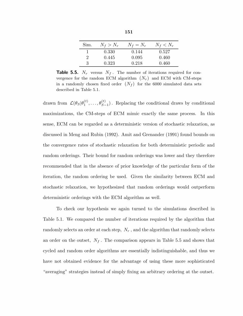
151

Sim. Nf > Nr Nf = Nr Nf < Nr

1 0.330 0.144 0.5272 0.445 0.095 0.4603 0.323 0.218 0.460

Table 5.5. Nr versus Nf . The number of iterations required for con-

vergence for the random ECM algorithm (Nr) and ECM with CM-steps

in a randomly chosen fixed order (Nf ) for the 6000 simulated data sets

described in Table 5.1.

drawn from L(θS|θ(t)1 , . . . , θ

(t)S−1) . Replacing the conditional draws by conditional

maximizations, the CM-steps of ECM mimic exactly the same process. In this

sense, ECM can be regarded as a deterministic version of stochastic relaxation, as

discussed in Meng and Rubin (1992). Amit and Grenander (1991) found bounds on

the convergence rates of stochastic relaxation for both deterministic periodic and

random orderings. Their bound for random orderings was lower and they therefore

recommended that in the absence of prior knowledge of the particular form of the

iteration, the random ordering be used. Given the similarity between ECM and

stochastic relaxation, we hypothesized that random orderings would outperform

deterministic orderings with the ECM algorithm as well.

To check our hypothesis we again turned to the simulations described in

Table 5.1. We compared the number of iterations required by the algorithm that

randomly selects an order at each step, Nr , and the algorithm that randomly selects

an order on the outset, Nf . The comparison appears in Table 5.5 and shows that

cycled and random order algorithms are essentially indistinguishable, and thus we

have not obtained evidence for the advantage of using these more sophisticated

“averaging” strategies instead of simply fixing an arbitrary ordering at the outset.

152

5.7. Discussion

5.7.1. Convergence Criteria

In this section, we will show how the standard “step length” criterion can be quite

misleading and discuss the sensitivity of the results of the previous sections to the

convergence criterion. In all the simulations except those of Section 5.6, we used

the standard step length criterion: ||θ(t) − θ(t−1)|| ≤ ǫ , which was useful for our

purposes both because of its popularity and because it underlies (5.2.3) which relates

the number of steps required for convergence to the spectral radius. In the context

of cycled ECM, however, this criterion can lead to difficulties. If each iteration of

cycled ECM is defined as one E-step followed by S CM-steps, then the resulting

sequence {θ(t) : t ≥ 0} is not a simple linear iteration even at convergence since

the mapping that maps θ(t) to θ(t+1) changes with t . The difficulty with this

is demonstrated in Figure 5.9, which is a representation of the mapping induced

on a subspace of Θ by three ECM algorithms each with a fixed ordering (the

smooth curves) and by the cycled ECM algorithm that combines them (the jagged

curve). The three ECM algorithms are listed in the first row of Table 5.2. This

is again an example of fitting a log-linear model to a partially classified 2 × 2 × 2

contingency table. The asterisks represent the sequences and show that the cycled

ECM algorithm tends to have larger steps. In fact, using the standard convergence

criterion, ||θ(t+1) − θ(t)|| ≤ ǫ , this cycled ECM algorithm took 50 times longer to

converge than any of the three ECM algorithms. This is in spite of the fact that all

153

the algorithms increased the loglikelihood at about the same rate. (Cycled ECM is

the solid line in Figure 5.10.) Since the loglikelihood is increased at each iteration

an alternative convergence criterion is L(θ(t+1)|Yobs) − L(θ(t)|Yobs) < ǫ , which is

more desirable in the context of maximum likelihood estimation as described in

Section 5.6.

This brings up the question of how sensitive the results of the simulations

are to the convergence criterion. Figure 5.11 shows the values on Nmin/Nmax (as

defined in Section 5.4) for the simulations in Table 5.1 using the step length criterion

with ǫ = 10−10 and loglikelihood criterion with ǫ = 10−8 . The loglikelihood

criterion leads to more smaller values of Nmin/Nmax than does the standard length

criterion. Thus, CM-step permutations appear to be more important when the

loglikelihood criterion is used. (The comparisons here are not strictly “fair” because

of the choices of the threshold ǫ . However, it is difficult to decide what is fair here,

and the impact of ǫ on the relative value Nmin/Nmax should be small as long as

ǫ is not too big.)

Certainly, the convergence criterion plays an important role in both simula-

tion and practice and thus must be chosen carefully. The fact that the step length

criterion failed in cycled ECM shows that the practitioner must be careful when

evaluating convergence of algorithms that change even in subtle ways at each it-

eration. Whenever possible, we recommend the use of the likelihood criterion, in

addition to the step length criterion.

154

Comparing the Mappings

theta 1

thet

a 2

0.12 0.14 0.16 0.18 0.20 0.22

0.08

0.10

0.12

0.14

0.16

0.18

0.20

*

* *

*

*

*

*

*

*

*

*

*******************************************************************************************************************************************

*

** *

*

*

*

*

*

*

*

*

*

*****************************************************************************************************************************************

*

**

*

*

*

*

*

*

*

*

*

**

**

********

******************************************************************************************************************************

*

**

* *

*

* *

*

* *

*

* *

*

**

**

*

***

***

***

***

* **

* **

* *** *** ***************************

******************************************************************************

Tracking the Likelihood

iteration

Logl

ikel

ihoo

d

0 50 100 150 200

-40.

0-3

9.8

-39.

6-3

9.4

-39.

2-3

9.0

-38.

8

Figure 5.9. The mapping induced by the cycled ECM

algorithm. The mapping induced on the parameter space

(cell probabilities) by three ECM algorithms (dotted lines)

and the composite cycled algorithm (solid line). Notice the

jagged step pattern of the cycled ECM algorithm.

Figure 5.10. Tracking the likelihood with the cycled

ECM algorithm. The figure shows how the four algo-

rithms mapped in Figure 5.9 increase the loglikelihood.

The fixed order ECM algorithms (upper dashed lines) are

indistinguishable and increase the loglikelihood somewhat

faster than the cycled algorithm (lower solid line).

155

0.0 0.2 0.4 0.6 0.8 1.0

0.0

0.2

0.4

0.6

0.8

1.0

Nmin/Nmax using the Length Criterion

Nm

in/N

max

usi

ng th

e Li

kelih

ood

Crit

erio

n

Effect of Convergence Criteria

.

.

.

.

.. ..

..

..

..

.

..

.

..

...

.

.

..

.

..

.

.

.

.

.

.

.

.

.. .

.

.. .

..

... .

.

.

...

..

..

.

..

.

...

.

.

.

.

..

.

..

.

.

.

.

.

..

..

.

.

..

.

..

.

.

.

.

.. .

.

..

.

.

.

..

.

.

.

.

.

.

..

.

.

.

.

.

. .

..

...

..

.

.

.

...

.

.

.

.

..

.. .

.

.

.

.

.

.

.

..

.

....

.

..

.

..

.

.

.

.

.

...

.

..

.

..

.

. ...

.

.

.

.

.

.

..

.

.

.

.

..

.

.

.

.

.

.

.. .

.

..

.

..

... .

.

.

.

.

..

.

.

...

... ..

.

.

.

.

.

.

.

.

.

.

.

.

.

..

.. .

.

.

.

..

...

.

.

..

.

.

.

..

..

.

..

.

.

....

..

.

..

.

.. .

. ..

...

.

.

. ..

.

.

..

.

..

.

..

..

.

...

.

..

..

.

.

.

..

.

.

.

.

..

.

.

....

.

.. ..

.

.

.

.

..

..

.

.

. .

.

.

.

.

..

.

.

..

.

.

.

.

.

.

.

.

.

.

.

.

.

.

.

.

..

.

.

.

.

.

. .

..

..

.

.

.

.

.

.

.

.

..

..

.. .

.

.

.

.

.

...

.

.

.

.

.

...

.

.

...

.

.

..

.

.

. .

.

.

.

.

.

.

.

.

.

.

.

.

.

..

...

.

.

..

.

..

.

.

.

.

.

..

..

.

.

.

.

...

.

.

.

. ..

.

. ...

.

.

.

. ...

.

.

... .

.

.

.

...

..

..

. ..

.. .

.

.

. .

..

.

.

.

.

.

.

.

..

.

.

.

..

.

.

. ..

. .

.... ..

.

.

.

.. .

. .

.

..

. ..

.

.

.

.

. .

.

.

.

.

.

.

.

..

.

.

.

.

.

.

..

... .

.

.

.

.

..

.

.

.

. .

.

.

..

..

...

...

.

.

.

.

.

.

.

.

.

.

.

..

.

.

...

.

.

.

.

..

.

..

.

..

.

.

.

.

.. .

.

.

..

..

.

.

. ...

. .

.

..

.

.

.

.

.

.

..

..

...

.

.

...

.. . ..

..

..

.

.

.

..

.

.

.

.

..

.

.

.

.

. .

.

.

..

. .. .

. ..

.. .

..

.

.

.

.

..

.

. .

.

...

..

.

.

.

.

..

.

..

..

.

.

.

.

.

.

.

.

.

.

..

.

.

.

.

.

.

.

.

.

.

..

.

.

.

.

.

.

.

. .

. .

.

.

..

.

..

.

.

. .

..

.

.

.

.

.

.

.

..

.

.

.

.

.

.

.

.

. .

..

.

.

..

.

.

.

.

...

.

.

.

.

..

...

.

... .

.

.

.

. ....

.

..

.

.

.

.

.

.

. .

.

.

.

.

.

.

.

.

.

.

.

.

.

.

.

....

.

..

.

.

.

.

.

.

.

.

.

...

.

..

.

.

.

... .

. .

..

.

...

.

.

.

..

...

.

.

.

.

.

.

.

.

.

.

.

.

.

..

.

..

.

.

..

..

..

.

.

.

.

..

.

.

.

.

...

.

.

.

.

...

.

.

.

.

.

..

.

.

. .

..

.

. ..

. . ... .

..

.

...

.

..

..

.

.

..

. ..

.

.

.

... . ..

.

.

.

..

..

.. .

.

..

...

..

.

.

.

.

.

.

. .

..

.

. .

.

.

.

. ..

..

.

.

.

.

.

.

.

..

...

.

.

.

.

.

.

.

.

. .

.

... .

. .

.

.

.

.

. .

.

.

..

.

.

.

.

.

.

.

..

.

.

..

.

..

.

..

.

.

..

.

.

.

.

.

.

.

.

.

...

.

.

..

.

..

.

.

..

.

.

.

.

.

.

.

.

.

.

.

..

.

.

.

.

..

.

.

.

.

..

.

.

.

..

..

..

.

.

.

.

.

..

.

.

..

..

..

...

....

.

.

..

..

..

.

..

. ...

.

.

.

. .

.. .

.

...

..

.

.

. . ..

.

.

. . .

. .

.

..

.

. .

.

. ..

.

.

.

... .

.

.

... .

.

.

.

..

.

. ..

.. ..

.

.

.. .

.

.

. ..

.

.

.

..

.

..

.

..

.

.

..

.

.

. ..

.

.

.

.

..

.

.

.

.

..

..

..

.

.

.

.

.. ..

..

.

.

.

.

..

.

.

.

..

.

.

.

. .

.

. ...

.

.

. .

.

....

.

.

.

.

..

. .

.

.

.

.

.

.

. .

.

.

..

.

.

.

..

...

.

..

.

..

.

..

.

..

.

.

.

..

..

.

.

.

.

.

..

.

.

..

..

.

. .

..

.

...

...

.

.

.. .

..

..

.

...

.

.

.

.

..

.

. .

..

.

...

..

.

.

..

......

.

..

. .

. ..

.

.

.

.

.. .

.

.

.

.

.

.

.

.

..

..

. .

.

. .

.

.

.

..

.

.

.

.

..

.

.

.

.

. ..

.

.

.. .

. .

.

..

.

.

.

.

...

.

.

......

..

.

.

.

..

..

.

..

.

.

... .

.

.

..

.

.

.. .

..

.

.

..

.

.

..

.

.

.. ..

.

.

.

.

..

...

..

.

.

.

.

.

..

..

. .

.

.

.

.

.

.

.

.

..

.

.

.

.

.

.. .

...

.

...

.

.

..

.

..

..

.

.

..

.

.

.

.

..

.

.

.

.. ... .

.

...

.

.

.

..

.

.

.

.... .

.

. ..

.

..

.. . ..

.

.

.. . .

..

.

.

.

.

..

.

....

..

..

.

..

.

.

..

.

.

.

.

...

.

. ..

..

.

.

. .. .

..

.

.

.

.

..

. ..

..

...

. ..

..

...

..

.

..

. ..

..

.

..

.

.

..

.

...

.

.

.

.

.

.

.

.

.

.

.

.

..

.

.. .

.

.

.

.

.

...

..

.

...

..

..

.

.

..

.

.

.

.

.

.... .

.

.

.

.

..

.. .

..

.

..

.

.

.

.

..

.

. .

. ..

. ...

.

.

..

..

. .

..

.

. .

.

.

.

.

.

.

.

.

. .

. .

.

.

.

. ..

.

.

.

. .

..

.

..

.

.

.

.

.

.

..

.

.

.

..

.

.

.

.

.

.

..

..

..

. .

.

.

.

.

.

.

.

..

.

.

..

.

..

..

.

.

.

..

.

..

..

.

. ...

..

..

.. .

.

.

..

.

.

.

.

.

.

.. .. .

..

.

...

..

.

.

.

.

.

.

. .

..

...

. ....

.

.

.

.

.

.

..

..

.. ..

.

.

.

......

.

.

..

.. .

.

...

.

.

.

..

.

..

.

. .

.

.

. ...

.

.

.. .

.

.

.

.

.

..

..

...

. .

.

.

..

.

...

.. ...

.

..

.

..

.

.

.

..

..

. ...

.

.

..

.

.

.. . .

.

..

.

..

.

.

..

.

... .

.

. .

..

.

.

.

.

.

...

..

.

.

. .

.

..

..

. .

.

.

.

..

.

.

..

.

. ...

.

.

.

...

...... .

.

... .

..

..

.

. .

.

..

.

.

..

. .

.

..

..

.

.

..

.

...

.

.

.

.

.

..

.

.. ..

..

..

... ..

.

.

.

.

..

.. ..

... .

..

..

..

. . ...

.

...

.

.

.

. ...... ..

.

.

.

.

.

.

..

.

... .....

. .

.

.

..

...

...

..... .

.

.

..

...

.. . ...

.

....

.

. .

.

..

.

..

.

.

.

..

.

.

.

.

..

.

....

..

.

...

.

.

.

.

..

..

..

.

.

.

.

..

..

.

.

.

.

..

.

.

.

..

.

.

..

.

...

..

.

.

..... .

.

.

.

..

..

..

.

.

..

..

..

.

.

.

. .

.

.

. .

.

...

.

.

.

.

.

.

.

.

....

.

..

.

.

..

.

....

.

.

.

.

.

..

.... .

..

..

...

.

..

..

.

.

.

..

..

.

.

.

...

.

. .

...

.

.

.

.

. .

.

.

.

.. .

..

.

..

.

.

.

.

. ..

.

.

..

..

.

..

.

.

.

..

..

.

...

..

.

. .

.

.

.

..

.

.

.

.

.

.

.

.

..

...

. .

...

.

.

. .

..

..

.

.

..

..

.

.

..

...

.

. .

.

.

.

.

..

.

..

.

.

.

. ..

.

.

.

.

..

..

.

.

..

..

.

..

.

..

.

.

. .

.

.

. ....

....

.

...

.

..

. ...

.

.

.

.

.

.

.

.

.

..

.

.

. ...

..

...

.

..

..

..

.

.

..

.

.

.

.. .

..

..

..

.

.

.

.

.

.

..

.

...

... ..

. .

...

.

..

..

.

..

.

.

..

.

.

.

.

.

.

.

.

.

.

.

...

.

..

..

.

.

..

...

.. ..

. .

.. .

..

.

..

.

.

. .

.

.

.

. .

.

. .

.

.

.

.

.

.

. .

.

..

.

..

.

.

.

.

.

.

.. .

.

. .

.

....

....

..

.. .. ..

.

.

..

..

.

.

.

.

..

.

.

.

..

..

. ..

..

...

.

.

...

.

.. ..

.

.

.

... .

.. .

..

.

..

..

.

.

..

.

.

..

.

..

. .

..

.

..

.

.

.

.

..

..

..

.

.

.

.

.

.

.

.

..

.

..

.

..

. ...

..

. . .

.

.. .

.

.

.

... ...

...

. ....

.

.

..

..

.

.

.

. . .

..

.

.

.

..

...

.

. .

.

..

..

.

..

.

.

.

..

.

. .

.

.

...

.

.

...

..

.

...

..

. ..

.

. .

..

..

.

.

.

.

.

.

.

...

..

.

...

..

.

.

.

. ..

. .

.

.

..

.

. .

..

..

.

.

.

....

.

.

...

.

.

..

. . ..

.

.

..

.

.

.

..

.

.

.

.

.

. ..

.

..

.... .. ..

.

.

....

..

.

. ..

.

..

.

.. .

..

.

.

.

.

..

..

.

.. .

.

.. ....

.

.

.......

.

.

..

.

..

..

.

.

.

..

.

..

.

.

..

.

....

.

.

. ..

.

.

..

.

.

.

..

.

....

.

.

... .

.

.

.

..

.

.

.

....

.

.

.

. .

.

..

.. .

.

.

..

.. ..

.

.

..

.

.

..

.. .

.

.

.

.

.

.

.. ... .

.

.

.

.

.

.. ..

.

.

..

.

.

.

.

.

..

..

.

. .

.

. .

.

. .

.

... .

....

.

.

..

.

.

.

.

.. .

....

..

.

...

.

.

.

.

..

...

.

.

.

.

.

..

.

.

.

.

.

..

. ..

.....

...

...

.

.

..

.

.

..

.

..

.

..

.

.

.. .

.

..

.

..

.

.

..

.. .

.

..

..

.

.

. .

..

.

.

.

.

....

.

.

..

.

. . .. .

..

...

.

.. .

.

.

.... ..

...

..

.

..

. ..

.

.

.

..

..

.

..

..

.

.

.

.

...

.

...

.

..

.

.

.

.. ..

.

. ...

.

.

.

.

...

.

.

.

.. .

..

.

.

.

..

.

.

..

.. ..

. ...

..

.

.

..

.

.

..

..

..

.

.

.

.

. .

.

.

.

...

.

...

.

..

.

....

..

..

.

.

.

. ..

. .

.

.

.

..

.

. ..

.

.

.

.

.

..

.

.

.

. .

.

.

.

.

.

. ..

..

..

...

...

..

.

.

.

...

.

.

..

.

..

.

.... ..

..

.

.

...

.

.

.

..

.

.

..

..

.

..

..

. ..

.

.

..

..

.

..

.

..

.

.

...

... .. .

.

.

.

.

...

. .

. .

.

.

.

.

.

.

. .

..

.

..

.. .

..

.

.

. .

.

.

..

.

...

.

.

.

...

..

..

.

...

.. .

. ..

. .

.. .

..

.

.

.

.

.

.

.

.. ..

.

.

.

.

.

.

.

.

...

.

. .

.

.

...

.

.

.

. .

.

..

.

..

.

.

..

.

. .

.

.

...

.

.

.

.

...

.

.

..

.

...

.

.

..

..

..

.

. .

.

.

.

.

.

..

.

..

. .

.

.

.

. .

.

.

.

.

.

.

.

.

..

.

.

..

..

.

.

..

.

....

.

.. ..

...

..

.

...

.

. .

.

..

..

.

..

.

...

..

.

..

.

.

.

.

.

. ...

.. .

.

..

..

.

. ..

.

..

.

..

.

.

.

..

.

. ..

.

..

.

.

.

..

.

.

..

..

.

..

.

....

.

.

...

.

..

.

.

.

.

.

.

.

.

. .

.

..

.

.. .

.

..

. ..

. ..

.

.

. .

.

.

.

.

.. ..

.

.

..

.

...

.

..

.

..

.

..

.

..

.

..

..

.

.

.

. .

..

.

..

..

..

...

.

.

..

..

. .

.

.

.

.

.

.

.

.

.

.

...

.

..

.

.

.

.

.

.

.

.

.

..

.

..

....

.

.

.

..

.

..

..

.

. .. .

.

..

.

.

.

...

.

.

.

.

.

..

.

.. .

..

..

.

.

.

.

. .. ..

..

..

.

..

.

.

.

. .

.

.

.

. .

.

.

.

.

.

. .

..

..

. ..

..

.. .

.

..

.

.

.

..

.

.

.

..

..

..

.

.

.

.

..

.

.

.

.

.

.

.

.

. .. .

.

.

.

.

.

.

.

. .

.

.

..

...

.

.

..

.

.

..

.

.

..

.

.

..

..

..

.

.

..

.

.

.

.

.

.. .

.

.

.

..

.

.

.

.

...

..

..

.

..

.

..

.

.

.

.

..

.

..

.

.

.

...

.

..

.

. .

..

.

.

.

.

.

. .

.

.

.

.

.

. .

.

.

.

..

.

..

..

.

.

.

.

..

...

.

.

.

.. ..

.

.

.

.

.

.

.

. ..

.

.

.

..

.

.

.

.

.

.

.

.

.

.

..

..

.

.

..

.

..

.

.

.

.

..

...

.

.

..

.

.

.

..

.

.

..

.

.

.

. .

..

.

.

.

.

.

.

.

.

.

.

.

.

. .

.

.

.

..

.

.

..

..

..

.

..

...

..

.

.

.

...

..

..

.

. .

.

.

.

.

.

..

.

.

.

.

..

.

... ..

..

..

.

..

.

.

..

.

.

. .

.

.

.

.

.

.

.

.

.

.

..

.

..

..

.

.

.

..

..

.

.

.

.

.

. .

..

...

..

...

.

.

..

..

.

..

.

..

.

...

..

.

.

..

.

.

.

...

.. ..

..

.

...

.

.

..

. ..

.

....

.

..

.

..

.

.

.

.

.

..

.

. ..

.

.

.

.

.

.

.

..

.

..

.

..

.

.

.

.

.

.

.

.

.

..

.

.

.

..

...

.

.

...

.

.

.

.

. ..

...

.

..

.

..

.

.

.

.

.

.

..

.

.

....

.

..

.

..

.

..

. .

..

.

.

.

.

.

.

.

.

.

..

..

.

.

.

.

..

.

.

. ..

.

.

...

.

..

.

..

.

..

.

..

.

.

.

. .

..

.

...

.

.

.

...

.

.

.

..

.

.

.

..

..

..

.

.

.

.

..

..

.

.. .

....

..

..

. .

.

.

..

..

.

. .

.

...

.

.

.

.

.

.

.

.

..

.

.

.

..

.

.

.

..

.

.

..

...

.

.

.

.

.

.

.

.

..

.

.

.

.

.

.

.

...

.

.

.

.

...

.

..

.

.

.

.

.

.

.

.

.

.

.

..

.

. .

.

.

.

..

. ..

.

.

.

.

. .

.

.

.

.

.

.

.

.

.

.

.

.

.

.

.

.

...

.

..

.

..

.

...

...

.

..

.

.

.

..

.

..

.

.

..

...

.

.

.

..

.

.

.

.

.

.

..

.

.

.

.

.

..

.

..

..

.

.

.

.

.

.

.

.

.

.

.

.

.

..

.

..

.

.

...

.

.

.

.

..

.

. ..

.

.

..

. ..

.

.

..

.

.

.

.

.

.

.

.

.

.

.

.

.

. ..

.

.

.

.

.

.

.

.

.

..

.

..

.

..

.

.

.

.

..

. .

.

..

..

.

...

.

.

..

.

.

.

.

..

.

.

.

.

.

..

.

.

.

. ..

.

..

.

.

.

.

.

..

.

. .

.

..

.

...

.

. .

. .

. .

.

.

.

.

.

.

.

.

.

..

.

..

...

.

.

.

..

.

.

.

. .

.

.

..

..

..

.

.

.

.

.

.

..

.

..

.

..

.

.

.

.. .

.

.

.

.

..

.

.

.

..

.

.

.

...

..

.

.

..

.

..

...

. .

.

.

.

.

..

.

. ..

.

..

.

.

.

...

.

.

.

. ..

.

.

.

.

.

...

..

..

.

..

.

.

.

...

.. .

.

.

.

...

.

.

. .

.

..

.

.

..

.

.

..

.

.

.

.

.

..

..

.

.

.

.

..

.

.

.

.

.

..

.

.

..

.

.

.

.

..

.

.

.

.

.

.

.

..

.

.

. ..

.

...

.

..

...

.

.

.

.

.

.

. ..

.

.

.

.. ..

.. .

. ..

.

.

.

.

....

.

.

.

.

.

.

.

.

.

..

. . .

.

.

.

.

.

.

..

..

.

.

..

...

..

.

.

..

..

.

.

.

.

.

.

.

.

.

.

.

.

.

..

.

..

.

.

.

..

.

.

.

. .

.

. .

.

.

.

.

..

.

.

..

.

.

.

.

.

.

.

.

.

.

.

. .

..

..

. .

..

.

..

.

.

.

.

.

.

.

.

.

.

.

.

.. .

.

..

.

.

..

.

.

.

.

.

..

.

.

.

.

.

.

.

..

..

.

..

..

.

..

.

..

.

..

..

.

..

.

.. .

.

. .

.

.

..

....

.

.

.

.

.

.

.

.

...

..

.

..

..

. .

.

..

.

.

.

.

...

.

.

.

.

..

.

.

..

..

..

.

.

..

.

.

.

.

..

..

.

.

.

.

.

.

..

.... .. .

.

.

.

.

..

.

..

.

.

.

...

.

..

. ..

..

.

..

.

..

..

. ..

.

.

.

. .

.

.. ..

.

.

.

.

..

. ...

.

.

.. .

.

.

.

.

.

.

..

.

. .

.

.

.

.

.

.

.

.

....

.

.

.

..

.

.

.

..

.

.

..

.

.

.

.

.

. ..

.. .

.

.

.

.

.

.

.

..

..

.

.

.

.

.

.

.

. ..

.

.

.

.

..

.

.

..

.

.

...

.

.

.

.

..

.

.

.

.. .. .

.

.

..

.

.

..

.

.

.

.

.

.

.

.

..

..

.

..

.

.

.

.

.

.

..

..

.

.

.

.

..

.

..

.

.

.

..

.. .

.

.

. ..

.

.

.

.

.

.

.

..

.

..

.

.

.

.

.

..

.

. ..

.

.

.

.

.

..

..

..

.

.

. . .

.

.

.

. ...

.....

.

.

.

.

.

..

.

..

.

. ..

.

.

.

.

.

.

.

..

..

.

.

.

.

.

..

..

.

.

.

.

.

.

.

..

.

.

.

.

.

.

.

.

.

.

.

.

.

.

.

.

.

.

.

.

.....

.

.

.

..

.

.

.

.

.

.

.

.

.

... .

.

..

.

.

.

.

. .

.

.

.

.

.

.

.

.

.

.

.

.

..

.

.

.

..

.

.

.

.

.

.

.

.

.

Figure 5.11. Compareing the loglikelihood and step length convergence

criteria. This is a plot of Nmin/Nmax using both criteria for the 6000 simu-

lations described in Table 5.1. Notice that the effect of CM-step permutation

tends to be larger with the loglikelihood criterion.

5.7.2. Stratagies for ordering CM-steps

The simulations presented in Sections 5.3 and 5.4 show that the effect of permuting

CM-steps on the number of iterations required for convergence can be much more

substantial than the theoretical results predict. This finding is rather informative

since most studies of the convergence of EM type algorithms have been conducted

purely with regards to the asymptotic character of the iteration. The result, how-

ever, is somewhat discouraging in light of how evasive exact analysis of the iteration

can be.

When considering the problem of ordering, perhaps the question of most

interest is how large the effect of ordering can be. We have seen that an increase

156

in efficiency of 20% is not uncommon in the 2 × 2 × 2 table. Other simulations

suggest that in problems with more CM-steps the effect tends to be larger. In the

contingency table setting, the sparseness of the table is also important. In tables

with less data, the effect of CM-step permutation can be greater. Effective strategies

for maximizing efficiency continue to be elusive. Neither relative amounts of missing

data nor characteristics of the subspaces onto which the CM-steps project (i.e.,

Alternating Projection Algorithm, Kayalar and Weinert, 1988) have been found

to be useful in determining a general technique for choosing an efficient ordering.

Based on our limited simulations, a user who is faced with a sparse table with

many CM-steps is perhaps best off randomly selecting the order of CM-steps at the

outset of running the algorithm. In general, when one is unsure if more sophisticated

strategies will pay off, we recommend randomly fixing an order of CM-steps before

implementing the ECM algorithm.

Finally, we emphasize that our general philosophy behind investigating the

effect of permuting CM-steps is to see if there is a “free and better lunch,” not

a “better but costly lunch” in terms of human and computational effort. Given

the diversity of applications of EM-type algorithms, it seems impossible to find an

“optimal” order-choosing rule that will be universally applicable. Even if such a rule

could be found, it has no practical value unless the savings it provides outweighs

the cost of implementing it. On the other hand, a practitioner may be interested in

knowing about strategies that will lead to relatively efficient algorithms in common

implementations of EM-type algorithms (e.g, ECM applied to contingency tables)

especially when the algorithm is slow to converge, and in what situations the issue

157

of ordering is not worth consideration because it is unlikely to have an appreciable

impact on the problem at hand. In either case, the practitioner is informed by a

general investigation that helps to answer these questions.

Chapter 6

The Global Rate of EM as an Inferential Tool:

Finite Mixtures

6.1. Finite Mixture Distributions

Finite mixtures appear in many areas of the statistical literature. The density of

the general finite mixture distribution is the weighted average of the k densities

(subpopulations) fi(y|βi) and can be formulated as

f(y|θk) =

k∑

i=1

αifi(y|βi), (6.1.1)

where∑αi = 1 and θk = (α1, . . . , αk, β1, . . . , βk) . Attempts to estimate the

parameters in (6.1.1) date back at least to Pearson’s (1894) method of moments

solution to a mixture of two univariate normals with different means and variances.

The algebra was formidable indeed, the first step of the solution requiring a neg-

ative root of a “nonic” equation. Since then graphical, likelihood, Bayesian, and

minimum density distance solutions have been proposed (see Titterington, Smith,

and Markov, 1985 for a nice review). Even when k is known, likelihood estimation

has generally been hindered by the fact that the loglikelihood does not take the

158

159

familiar additive form. A simple yet general computational strategy, however, is

to apply the EM algorithm, treating the subpopulation memberships (i.e., mixture

indicator) as missing data.

The mixture problem is further complicated when the number of subpop-

ulations k is unknown, and thus needs to be estimated. The two facts that k

is discrete and that supθk∈Θk

f(y|θk) is nondecreasing in k make estimation of k

a nontrivial task. There is a diverse and creative literature of attempts to solve

this rather challenging estimation and the related testing problems. Noticing that

f(y|θk+1) is a just f(y|θk) with αk+1 = 0 (or fk+1(y|βk+1) = fk(y|βk) ), Wolfe

(1970) proposed using the likelihood ratio test with its standard asymptotic distri-

bution. It was pointed out later, however, that the fact that the constrained space

is on the boarder of the parameter space destroys the standard asymptotic result.

Others have suggested methods based on the chi-square distance from the empiri-

cal CDF (Henna, 1985), modified likelihood ratio tests (Aitkin and Rubin, 1985),

Monte Carlo estimation (Aitkin, Anderson and Hinde, 1981), graphical techniques

(c.f., Titterington, Smith and Makov , 1985), and order statistics (Maine, Boullion,

and Rizzuto, 1991).

One particularly interesting approach was proposed by Windham and Cutler

(1992), in which the rate of convergence of EM is used to estimate k . As we have

seen, the larger the augmented information (relative to the observed information),

the slower the EM algorithm converges. In the mixture problem, EM is run condi-

tional on an assumed k and the augmented data is {(yi, zi), i = 1, . . . n} , where zi

indicates the subpopulation membership of observation yi . Windham and Cutler

160

(1992) argued that if the assumed k is too large or too small compared to the

underlying true k , the subpopulation memberships are “ill-defined” making the

algorithm slow. Thus, after running several EM algorithms with different values of

k(≥ 2) , they propose to estimate k as the number of subpopulations that results

in the fastest EM algorithm. This idea suggests that the augmented-data loglike-

lihood contains information for the parameter k beyond what is contained in the

observed-data loglikelihood.

Windham and Cutler’s argument for this method was largely heuristic and

their evidence came from a single example. Nevertheless, the idea is not only novel

but also if successful has great potential in EM application outside of finite mixture

models. In this chapter, we will continue to explore the usefulness as well as the

limitations of this method. In Section 6.2, we introduce the necessary details of the

EM algorithm used to fit finite mixture models and its rate of convergence and in

Section 6.3 we briefly review the details of Windham and Cutler (1992). In Sec-

tion 6.4, we show that Windham and Cutler’s approach can be viewed as a minimax

estimator. We then discuss the large-sample behavior of the estimator, conducting

an empirical study (Section 6.5) and presenting a more theoretical argument (Sec-

tion 6.6), both of which indicate that the estimator can be inconsistent and tends to

underestimate the true k . Finally, Section 6.7 proves several propositions presented

in Section 6.6 and presents an outline of a more thorough theoretical investigation.

161

6.2. Using EM to Fit Finite Mixture Models

As described in Dempster, Laird, and Rubin (1977), to implement the EM algorithm

in the context of finite mixture analysis, we augment each of the observed-data

points, yi with its (unknown) subpopulation membership, zi , where zij is the

indicator function of whether yi belongs to subpopulation j . We will label the

observed values Yobs = {y1, . . . , yn} and the augmented data Yaug = {(yi, zi), i =

1, . . . , n} . Given a working model f(y|θk) we can write the expected augmented-

data loglikelihood

Q(θk|θ(t)k ) =

∫L(θk|Yaug)f(Ymis|Yobs, θ

(t)k )dYmis. (6.2.1)

Since this function is linear in {zij , i = 1, . . . , n} , the E-step amounts to computing

E[zij |Yobs, θ(t)k ] =

α(t)j fj(yi|β(t)

j )∑k

l=1 α(t)l fl(yi|β(t)

l ), j = 1, . . . , k, i = 1, . . . , n, (6.2.2)

which is simply P(zij = 1|θ(t)k , yi) . The M-step then maximizes Q(θk|θ(t)

k ) , a com-

putational task that is the same as maximizing the augmented-data loglikelihood

L(θk|Yaug) , with zij replaced by the probability found in (6.2.2).

In the context of the mixture problem, both the matrix rate DMEM and the

global rate r will depend on the working model f(y|θk) and thus on k , as well as

on the data and thus the true model f(y|θk0) , where k0 may be different from k

(here we assume that the true model is indeed a finite mixture). Since k and k0 are

of primary interest here, we will write the matrix rate DMEMn (k|k0) and the global

rate (i.e., the largest eigenvalue of DMEMn (k|k0) ) rn(k|k0)

† , where n indexes the

† The subscript on r will always be the sample size in this chapter and shouldnot be confused with the subscript on rt as defined in (1.6.9), which indicates theiteration number in the computational formula for r .

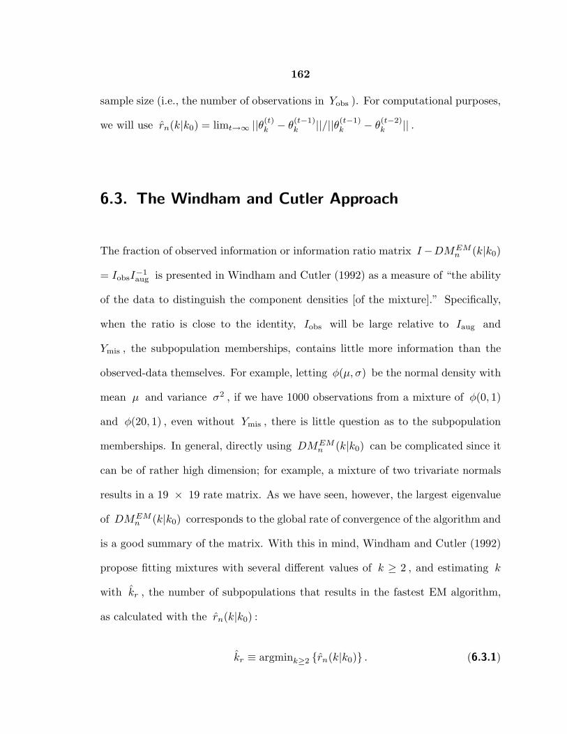
162

sample size (i.e., the number of observations in Yobs ). For computational purposes,

we will use rn(k|k0) = limt→∞ ||θ(t)k − θ

(t−1)k ||/||θ(t−1)

k − θ(t−2)k || .

6.3. The Windham and Cutler Approach

The fraction of observed information or information ratio matrix I−DMEMn (k|k0)

= IobsI−1aug is presented in Windham and Cutler (1992) as a measure of “the ability

of the data to distinguish the component densities [of the mixture].” Specifically,

when the ratio is close to the identity, Iobs will be large relative to Iaug and

Ymis , the subpopulation memberships, contains little more information than the

observed-data themselves. For example, letting φ(µ, σ) be the normal density with

mean µ and variance σ2 , if we have 1000 observations from a mixture of φ(0, 1)

and φ(20, 1) , even without Ymis , there is little question as to the subpopulation

memberships. In general, directly using DMEMn (k|k0) can be complicated since it

can be of rather high dimension; for example, a mixture of two trivariate normals

results in a 19 × 19 rate matrix. As we have seen, however, the largest eigenvalue

of DMEMn (k|k0) corresponds to the global rate of convergence of the algorithm and

is a good summary of the matrix. With this in mind, Windham and Cutler (1992)

propose fitting mixtures with several different values of k ≥ 2 , and estimating k

with kr , the number of subpopulations that results in the fastest EM algorithm,

as calculated with the rn(k|k0) :

kr ≡ argmink≥2 {rn(k|k0)} . (6.3.1)

163

The restriction k ≥ 2 is needed because when k = 1 , there is no missing data

and DMEM (1|k0) = 0 . Thus, we will only consider nontrivial mixtures. It should

also be mentioned that Windham and Cutler define kr as the k that maximizes

1 − rn(k|k0) , which they call the minimum information ratio (MIR).

Windham and Cutler’s basic justification for this procedure, in addition to

the heuristic argument presented above, was the application to a mixture of three

spherical bivariate normals with known and equal standard deviation. When the

standard deviation was small relative to difference in means, it is not surprising that

the method worked well (almost any method would work well). When the standard

deviation was relatively large, however, their tables reveal that kr picked the true

value of k only about half the time and underestimated almost every other time.

As we will see, this pattern continues in other examples.

To fully understand and explore this idea, we conducted both theoretical

and simulation studies, with a focus on constructing possibly better estimating

procedures.

6.4. The Rate Function and the Minimaxity of kr

It is clear from (1.6.2) – (1.6.5) that rn(k|k0) is attempting to measure differences

between the observed-data loglikelihood function, L(θk|Yobs) and the projection

of the augmented-data loglikelihood onto the observed-data space, i.e., the condi-

tional expectation of the augmented-data loglikelihood, Q(θk|θ⋆k) , where θ⋆

k is the

164

maximum likelihood estimate of θk . It remains unclear, however, what specific

properties it is measuring, or if what it is measuring is an appropriate basis for es-

timating k0 . In this section we introduce a more general and direct measure of the

difference between L(θk|Yobs) and Q(θk|θ⋆k) , inspired by rn(k|k0) . Specifically,

we define the rate function as

R(θ|Yobs) = 1 − L(θ⋆|Yobs) − L(θ|Yobs)

Q(θ⋆|θ⋆) −Q(θ|θ⋆), (6.4.1)

where θ⋆ is the limit of an EM sequence. (We have suppressed the subscript

k because the theory is general.) In order to gain an intuition for the numerical

properties of this function, we generated 10 000 observations from Yobs ∼ 12φ(0, 1)+

12φ(3, 1) , used EM to fit the model Yobs ∼ αφ(µ1, σ)+ (1−α)φ(µ2, σ) and plotted

(6.4.1) as a function of each of the four parameters fixing the other three at their

MLE (see Figure 6.1). The wild fluctuations of R(θ|Yobs) near the θk = θ⋆k are due

to numerical inaccuracy as the denominator in (6.4.1) approaches zero. The actual

plot near θ⋆ can be interpolated as a smooth function. We would like to compare

R(θ|Yobs) with the rate of convergence of EM, which is plotted as the horizontal

dashed line on each of the plots. From the plots, we see R(θ|Yobs) is always in the

unit interval, that the limθ→θ⋆ R(θ|Yobs) does not exist, and that each of the limits

along the axes of Θ are different but are less than the rate of convergence of EM.

Theorem 6.1 clarifies these properties.

Theorem 6.1: If θ⋆ is the global maximizer of L(θ|Yobs) then the function

R(θ|Yobs) defined in (6.4.1) has the following property

(1) 0 ≤ R(θ|Yobs) ≤ 1 for all θ ∈ Θ .

Furthermore, if ∇L(θ|Yobs)∣∣∣θ=θ⋆

= ∇Q(θ|θ⋆)∣∣∣θ=θ⋆

= 0 , then

165

0.0 0.2 0.4 0.6 0.8 1.0

0.0

0.2

0.4

0.6

0.8

1.0

MLE

0.6 0.8 1.0 1.2 1.4

0.0

0.2

0.4

0.6

0.8

1.0

MLE

-4 -2 0 2 4

0.0

0.2

0.4

0.6

0.8

1.0

MLE

-2 0 2 4 6 8

0.0

0.2

0.4

0.6

0.8

1.0

MLE

R(α

|Yobs)

α

R(σ

2|Y

obs)

σ2

R(µ

1|Y

obs)

µ1

R(µ

2|Y

obs)

µ2

Figure 6.1. Plotting R(θk|Yobs) as a function of θk . The solid lines

represent R(θk|Yobs) as a function of each of the components of θk with the

other components fixed at their MLEs. These are compared with the dashed

line which represents the rate of convergence of the EM algorithm. The limit

as θk approaches θ⋆k along each of the axes are rates of convergence of the

conditional EM algorithms and are different.

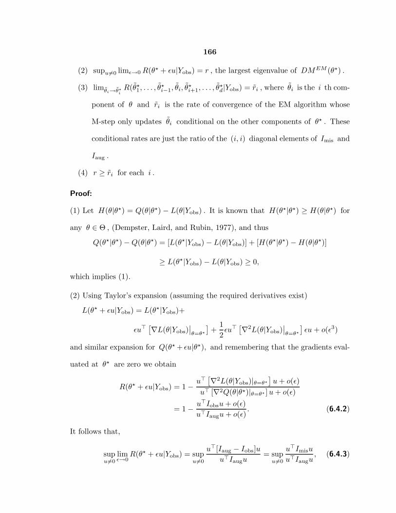
166

(2) supu6=0 limǫ→0R(θ⋆ + ǫu|Yobs) = r , the largest eigenvalue of DMEM (θ⋆) .

(3) limθi→θ⋆iR(θ⋆

1, . . . , θ⋆i−1, θi, θ

⋆i+1, . . . , θ

⋆d|Yobs) = ri , where θi is the i th com-

ponent of θ and ri is the rate of convergence of the EM algorithm whose

M-step only updates θi conditional on the other components of θ⋆ . These

conditional rates are just the ratio of the (i, i) diagonal elements of Imis and

Iaug .

(4) r ≥ ri for each i .

Proof:

(1) Let H(θ|θ⋆) = Q(θ|θ⋆) − L(θ|Yobs) . It is known that H(θ⋆|θ⋆) ≥ H(θ|θ⋆) for

any θ ∈ Θ , (Dempster, Laird, and Rubin, 1977), and thus

Q(θ⋆|θ⋆) −Q(θ|θ⋆) = [L(θ⋆|Yobs) − L(θ|Yobs)] + [H(θ⋆|θ⋆) −H(θ|θ⋆)]

≥ L(θ⋆|Yobs) − L(θ|Yobs) ≥ 0,

which implies (1).

(2) Using Taylor’s expansion (assuming the required derivatives exist)

L(θ⋆ + ǫu|Yobs) = L(θ⋆|Yobs)+

ǫu⊤[∇L(θ|Yobs)

∣∣θ=θ⋆

]+

1

2ǫu⊤

[∇2L(θ|Yobs)

∣∣θ=θ⋆

]ǫu+ o(ǫ3)

and similar expansion for Q(θ⋆ + ǫu|θ⋆), and remembering that the gradients eval-

uated at θ⋆ are zero we obtain

R(θ⋆ + ǫu|Yobs) = 1 − u⊤[∇2L(θ|Yobs)|θ=θ⋆

]u+ o(ǫ)

u⊤ [∇2Q(θ|θ⋆)|θ=θ⋆ ]u+ o(ǫ)

= 1 − u⊤Iobsu+ o(ǫ)

u⊤Iaugu+ o(ǫ). (6.4.2)

It follows that,

supu6=0

limǫ→0

R(θ⋆ + ǫu|Yobs) = supu6=0

u⊤[Iaug − Iobs]u

u⊤Iaugu= sup

u6=0

u⊤Imisu

u⊤Iaugu, (6.4.3)

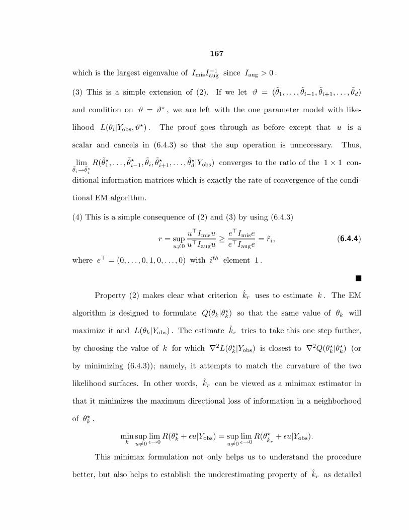
167

which is the largest eigenvalue of ImisI−1aug since Iaug > 0 .

(3) This is a simple extension of (2). If we let ϑ = (θ1, . . . , θi−1, θi+1, . . . , θd)

and condition on ϑ = ϑ⋆ , we are left with the one parameter model with like-

lihood L(θi|Yobs, ϑ⋆) . The proof goes through as before except that u is a

scalar and cancels in (6.4.3) so that the sup operation is unnecessary. Thus,

limθi→θ⋆

i

R(θ⋆1 , . . . , θ

⋆i−1, θi, θ

⋆i+1, . . . , θ

⋆d|Yobs) converges to the ratio of the 1 × 1 con-

ditional information matrices which is exactly the rate of convergence of the condi-

tional EM algorithm.

(4) This is a simple consequence of (2) and (3) by using (6.4.3)

r = supu6=0

u⊤Imisu

u⊤Iaugu≥ e⊤Imise

e⊤Iauge= ri, (6.4.4)

where e⊤ = (0, . . . , 0, 1, 0, . . . , 0) with ith element 1 .

Property (2) makes clear what criterion kr uses to estimate k . The EM

algorithm is designed to formulate Q(θk|θ⋆k) so that the same value of θk will

maximize it and L(θk|Yobs) . The estimate kr tries to take this one step further,

by choosing the value of k for which ∇2L(θ⋆k|Yobs) is closest to ∇2Q(θ⋆

k|θ⋆k) (or

by minimizing (6.4.3)); namely, it attempts to match the curvature of the two

likelihood surfaces. In other words, kr can be viewed as a minimax estimator in

that it minimizes the maximum directional loss of information in a neighborhood

of θ⋆k .

mink

supu6=0

limǫ→0

R(θ⋆k + ǫu|Yobs) = sup

u6=0limǫ→0

R(θ⋆kr

+ ǫu|Yobs).

This minimax formulation not only helps us to understand the procedure

better, but also helps to establish the underestimating property of kr as detailed

168

in the next sections. Although we could have discussed this minimax in terms

of DMEMn (k|k0) directly by using the first equality in (6.4.4), the formulation

of R(θ|Yobs) is interesting in its own right, lends insight into Windham and Cut-

ler’s approach and may lead to improved estimation procedures as discussed in

Section 6.6.

6.5. Large-Sample Behavior of kr – Empirical Results

Based on Windham and Cutler’s results, we suspect that kr may tend to underesti-

mate the actual number of subpopulations, k0 . In this section we will provide simu-

lation evidence that kr indeed underestimates k0 . In order to show this, our strat-

egy is to approximate r(k|k0) by rn(k|k0) when n is large enough so that we can

ignore the error in this approximation, and then to show that argmink≥2{rn(k|k0)}

is not necessarily k0 . To accomplish this we ran a simulation which drew n obser-

vations from Yobs ∼ 13φ(0, 1) + 1

3φ(δ, 1) + 1

3φ(2δ, 1) . The simulation was repeated

for 90 values of δ between 1 and 10 and for n = 1000, 10 000 and 100 000 . For

each data set EM was run to fit the model

Yobs ∼k∑

j=1

αjφ(µj , 1),∑

αj = 1, (6.5.1)

with k = 2 and rn(2|3) was calculated and is plotted for each n as a function of

δ in Figure 6.2 (the solid line corresponds to n = 100 000 ). The plot demonstrates

that rn(2|3) is converging as n increases and that r100 000(2|3) offers a reason-

able Monte Carlo approximation of r(2|3) (i.e., the following comparison can be

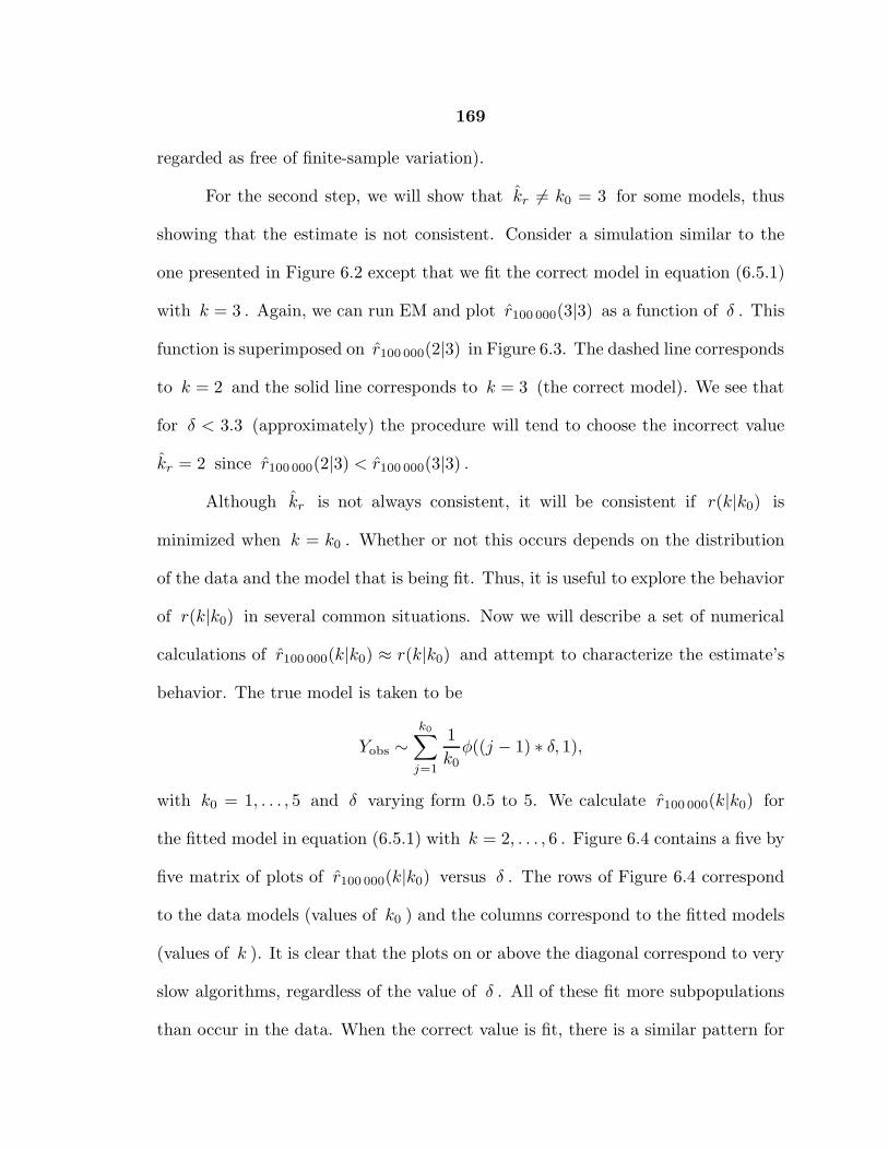
169

regarded as free of finite-sample variation).

For the second step, we will show that kr 6= k0 = 3 for some models, thus

showing that the estimate is not consistent. Consider a simulation similar to the

one presented in Figure 6.2 except that we fit the correct model in equation (6.5.1)

with k = 3 . Again, we can run EM and plot r100 000(3|3) as a function of δ . This

function is superimposed on r100 000(2|3) in Figure 6.3. The dashed line corresponds

to k = 2 and the solid line corresponds to k = 3 (the correct model). We see that

for δ < 3.3 (approximately) the procedure will tend to choose the incorrect value

kr = 2 since r100 000(2|3) < r100 000(3|3) .

Although kr is not always consistent, it will be consistent if r(k|k0) is

minimized when k = k0 . Whether or not this occurs depends on the distribution

of the data and the model that is being fit. Thus, it is useful to explore the behavior

of r(k|k0) in several common situations. Now we will describe a set of numerical

calculations of r100 000(k|k0) ≈ r(k|k0) and attempt to characterize the estimate’s

behavior. The true model is taken to be

Yobs ∼k0∑

j=1

1

k0φ((j − 1) ∗ δ, 1),

with k0 = 1, . . . , 5 and δ varying form 0.5 to 5. We calculate r100 000(k|k0) for

the fitted model in equation (6.5.1) with k = 2, . . . , 6 . Figure 6.4 contains a five by

five matrix of plots of r100 000(k|k0) versus δ . The rows of Figure 6.4 correspond

to the data models (values of k0 ) and the columns correspond to the fitted models

(values of k ). It is clear that the plots on or above the diagonal correspond to very

slow algorithms, regardless of the value of δ . All of these fit more subpopulations

than occur in the data. When the correct value is fit, there is a similar pattern for

170

0 2 4 6 8 10

0.0

0.4

0.8

0 2 4 6 8 10

0.0

0.4

0.8

Figure 6.3. The estimator kr is not consistent. The solid line approximates

r(3|3) and the dashed line r(2|3) . Since r(2|3) < r(3|3) for δ < 3.3 the

estimator kr is not consistent.

Figure 6.2. The convergence of rn(k|k0) . The three lines show rn(2|3)as a function of δ for several values of n (dotted: n = 1000 , dashed:

n = 10 000 , solid: n = 100 000 ). The convergence of rn(2|3) as nincreases is clear.

r n(2|3

)

δ

r n(k|3

)

δ

171

0.0

0.2

0.4

0.6

0.8

1.0

k=2

ko=1

number of subpopulations fit

true

num

ber

of s

ubpo

pula

tions

k=3 k=4 k=5 k=6

0.0

0.2

0.4

0.6

0.8

1.0

ko=2

0.0

0.2

0.4

0.6

0.8

1.0

ko=3

0.0

0.2

0.4

0.6

0.8

1.0

ko=4

0 1 2 3 4 5

0.0

0.2

0.4

0.6

0.8

1.0

ko=5

delta

0 1 2 3 4 5

delta

0 1 2 3 4 5

delta

0 1 2 3 4 5

delta

0 1 2 3 4 5

delta

Figure 6.4. ANOVA. The plots analyze the effect of the true number of

subpopulations ( k0 ), the fitted number of subpopulations ( k ), and δ on

r(k|k0) . Although kr tends not to overestimate k0 , it will often under-

estimate it when δ is small. The plots in the top row do not depend on δsince the model does not involve δ when there is only one subpopulation.

172

all of the values of k0 . The algorithm converges quite slowly if δ is less than about

2.5 and then begins to converge more quickly, converging rather fast at δ = 5 .

The situation is more complicated when we fit models that are too small. It is not

uncommon for these models to converge faster than the true model (especially for

k = 2 ). Figure 6.5 superimposes the plots with the same value of k0 , the actual

number of subpopulations. The solid lines correspond to fitting the correct model,

the dotted lines to models that are too big and the dashed lines to models that

are too small. It is evident from the plot that when δ is small, it is not at all

uncommon for one of the smaller models to converge faster than the true model

(this is especially clear when k0 = 4 ). Thus, kr will generally not pick the correct

value of k0 when there are several subpopulations and δ is small, no matter how

much data is observed.

One final aspect of the simulations warrants our attention. It seems reason-

able to expect the algorithms to converge more quickly as δ grows. This, however,

is not always the case when k < k0 . This is especially clear for k0 = 3 and k = 2

(see Figure 6.2), for which there are two critical points, at which the curve changes

its monotonicity. To understand what is happening, remember that the data fall

into three groups but the model is only fitting two. What is to be done with the

data in the third group? One of two things: either it is combined with one of the

other subpopulations, or it is split between both subpopulations. For small values

of δ , the subpopulations overlap very much and it works well to split the middle

group. As δ grows, however, this becomes more difficult and we observe the first

critical point ( δ ≈ 2.5 ). As δ continues to grows the subpopulations become more

173

0 1 2 3 4 5

0.0

0.2

0.4

0.6

0.8

1.0

delta

r(k|

2)

True Number of Subpopulations = 2

0 1 2 3 4 5

0.0

0.2

0.4

0.6

0.8

1.0

delta

r(k|

2)

True Number of Subpopulations = 3

0 1 2 3 4 5

0.0

0.2

0.4

0.6

0.8

1.0

delta

r(k|

2)

True Number of Subpopulations = 4

0 1 2 3 4 5

0.0

0.2

0.4

0.6

0.8

1.0

delta

r(k|

2)

True Number of Subpopulations = 5

Figure 6.5. Estimating k with kr . The plots show how well different

models fit for each of four values of k0 . The solid line represents the correct

model, dashed lines models that are too small, and the dotted lines models

that are too big. Minimizing r(k|k0) will often result in models that are

too small.

174

0 2 4 6 8 10

0.0

0.2

0.4

0.6

0.8

1.0

Figure 6.6. Splitting and combining subpopulations. When we fit a model

that has too few components some of the subpopulations will be either split

or combined. This plot shows how this is reflected in r(k|k0) . The dotted

line is r10 000(2|3) of Figure 6.2, the solid lines are α⋆ and 1 − α⋆ , and

the dashed lines are at 1/2 and 1/3 . For δ < 5 the middle subpopulation

is being split, for δ > 5 two subgroups are being combined.

αandr 1

0000(2|3

)

δ

distinct, the algorithm stops splitting the middle subpopulation and begins to com-

bine it with one of the others, and we observe the second critical point ( δ = 5 ).

This can be seen clearly by plotting the fitted value of α as a function of δ (Fig-

ure 6.6). Notice that for values of δ less than about 5, α⋆ is near one half because

the middle population is being split. For larger values of δ , α⋆ is near one third

because two subpopulations are being combined.

The empirical studies have illuminated an important characteristics of kr . It

tends to underestimate the true number of subpopulations because it is influenced

175

not so much by k0 as it is by the number of subpopulations salient in the observed

data. This characteristic will be the topic of the next section.

6.6. Large-Sample Behavior of kr – Discussion

In order to understand the Windham and Cutler method, we must carefully ana-

lyze the data-augmentation scheme. When the EM algorithm converges fast, the

subpopulation memberships are salient in the observed data. That is, when the

subpopulations have little overlap, the augmented data will contain little informa-

tion that is not contained in the observed data. On the other hand when there is a

lot of overlap among the subpopulations, the EM algorithm will require much data

augmentation, and will converge slowly. This will be formalized by two propositions.

The propositions consider what happens to the Fisher information matrices

that determine the rate of convergence of EM when the fitted number of subpopu-

lations results in a salient separation of the data (proposition 1) and a separation

that is not salient at all (proposition 2). In particular, we will consider the ex-

pected subpopulation memberships z⋆ = {z⋆ij , i = 1, . . . , n, j = 1, . . . , k} , where

z⋆ij = E[zij |Yobs, θ

⋆] , which can be represented by an n × k matrix with elements

on the unit interval such that∑k

j=1 z⋆ij = 1 for each i . (We denote such a ma-

trix space by Zn×k .) By a salient separation of the data, we mean z⋆ is close

to the boundary of Zn×k (i.e., matrices with only zero or one elements satisfying

the constraint∑

j zij = 1 for each i ). A set of subpopulations which result in

176

a separation of the data that is far from salient can be represented by z⋆ “deep

inside”Zn×k , for example z⋆ij = 1

k for each i and j . The two propositions look

at these two extremes for z⋆ in detail.

Proposition 1: Suppose f(y|θk) =∑k

j=1 αjg(y|βj) , where g(y|β) is twice differ-

entiable in the scalar parameter β , the normal equations are satisfied at the MLE

of θk , and z⋆ is on the boundary of Zn×k , then

Iobs = Iaug.

Proposition 2: Suppose f(y|θk) =∑k

j=1 αjg(y|βj) , where g(y|β) is twice differ-

entiable in the scalar parameter β , and z⋆ has two rows identical, then

|Iobs| = 0.

The proofs of the proposition will be presented in Section 6.7. The first proposi-

tion suggests that if the subpopulations are salient in the observed data, EM will

converge very quickly. The second suggests if there is no information to distinguish

between two subpopulations in the observed data, EM will converge very slowly.

Although both of the propositions assume the subpopulations densities differ only

in the value of a scalar parameter, a close look at the proofs suggests that they

could be generalized.

Several informal observations can be made based on these propositions. First,

kr does not estimate the true number of subpopulations but rather determines the

number of subpopulations that results in the most salient (per the above definition)

division of the data. We see this in action in Figure 6.6. Note that when δ is about

177

5, and the middle subpopulation is being split between the two subpopulations in

the model, EM converges very slowly since the observations in the middle population

could easily have come from either of the subpopulations. When δ grows a little,

however, we see EM converging much more quickly as a more salient division of the

data is possible – namely, combining two of the populations into one in the model. A

second observation is that even with large data sets kr will not be a good estimate

of the true number of subpopulations. If two or more of the subpopulations have

heavy overlap, more data will not help to separate them (i.e., the z⋆ij will not go

to zero or one as n increases).

Although kr may not be a good estimator of the number of subpopulations,

it is not without merit. As we have seen, rn(k|k0) is a good measure of how

well the data can be broken into k subgroups. Trying to minimize this quantity,

however, may not be the best strategy. After all, any data set falls nicely into one

population, and any well separated mixture with k0 = 4 will separate nicely into

two or three subpopulations. Thus, a large value of k that results in reasonable

convergence may be a good estimate of k0 , even if it does not result in the most

salient separation of the data (i.e., minimizing rn(k|k0) ). Reading across the rows

of Figure 6.4 indicates that taking k as large as possible such that EM does not

converge pathologically slow often results in a good estimate. To see why this is

true, suppose k > k0 , in which case we are fitting several parameters for which

there are really no observed Fisher information. Thus, L(θk|Yobs) will be very flat

along these parameters, and the rate function will be nearly 1 as θk approaches θ⋆k

in these directions. Thus, by (2) of Theorem 6.1, rn(k|k0) will be nearly 1 and EM

178

will be very slow to converge. For k ≤ k0 , on the other hand, the EM algorithm

generally converges reasonably well if k results in a reasonably salient separation

of the data. Thus, estimating k as the largest value which does not result in

pathologically slow convergence often leads to a good estimate of k0 . Of course,

this procedure may not be well defined in some cases since “pathologically slow”

may be a relative term. In our experience, however, fitting too many subpopulations

leads to very ill-behaved values of rn(k|k0) , which not only were large but also did

not converge well as t increased.

In summary, it seems likely that these procedures will tend to underestimate

the true k . Although this underestimation is less than ideal, it perhaps is the

best we can hope for and in fact may be a good reflection of the behavior of the

observed data. As is well known, when dealing with real data, all we can hope for

is to detect a few major mixture components, which fortunately is often enough for

the purpose of inference. In any case, mixture models for real data can only be

viewed as a useful approximation that help to identify some important underlying

heterogeneous groups.

One shortcoming in both our simulations and the example in Windham and

Cutler (1992) is that the variance structure was known, and not estimated from

the data. There are many difficulties in implementation that are avoided when

only location parameters are estimated. The likelihood for finite mixtures tends to

be very badly behaved with multi-modalities and unidentifiable parameters. These

difficulties tend to be more acute when scale parameters are estimated from the

data. In preliminary studies in this context, we have found that there are indeed

179

many modes of the likelihood function and that the rate of convergence can be

difficult to calculate (i.e., rt , as defined in (1.6.9), does not converge well) and

varies from mode to mode, especially when k > k0 . It is important, therefore, that

we are not quick to generalize our findings to the unknown scale problem before

more work is done.

Finally, it is important to note that the idea of using the rate of convergence

to help select a model is not limited to fitting finite mixture distributions. For

example, it could be used to estimate the number of factors in factor analysis. If

an approach can be shown to be effective in the context of mixtures, it is likely to

be useful in other applications involving estimating the number of latent variables.

6.7. Theoretical Development

6.7.1. Proof of propositions 1 and 2

Proof of Proposition 1: In this proof we will write the observed information in

terms of z⋆ij and α⋆

j using the relationship

z⋆ij

α⋆j

=g(yi|β⋆

j )

f(yi|θ⋆), j = 1, . . . , k, i = 1, . . . , n, (6.7.1)

which follows from evaluating (6.2.2) at θ(t) = θ⋆ . We will then evaluate the

observed information at z⋆ ∈ B(Zn×p) , the boundary of Zn×p to show that Iaug =

Iobs . In this and the next proof, we will suppress the subscript k on the parameter

θ to avoid confusion with the parameter subscripts which index the subpopulations.

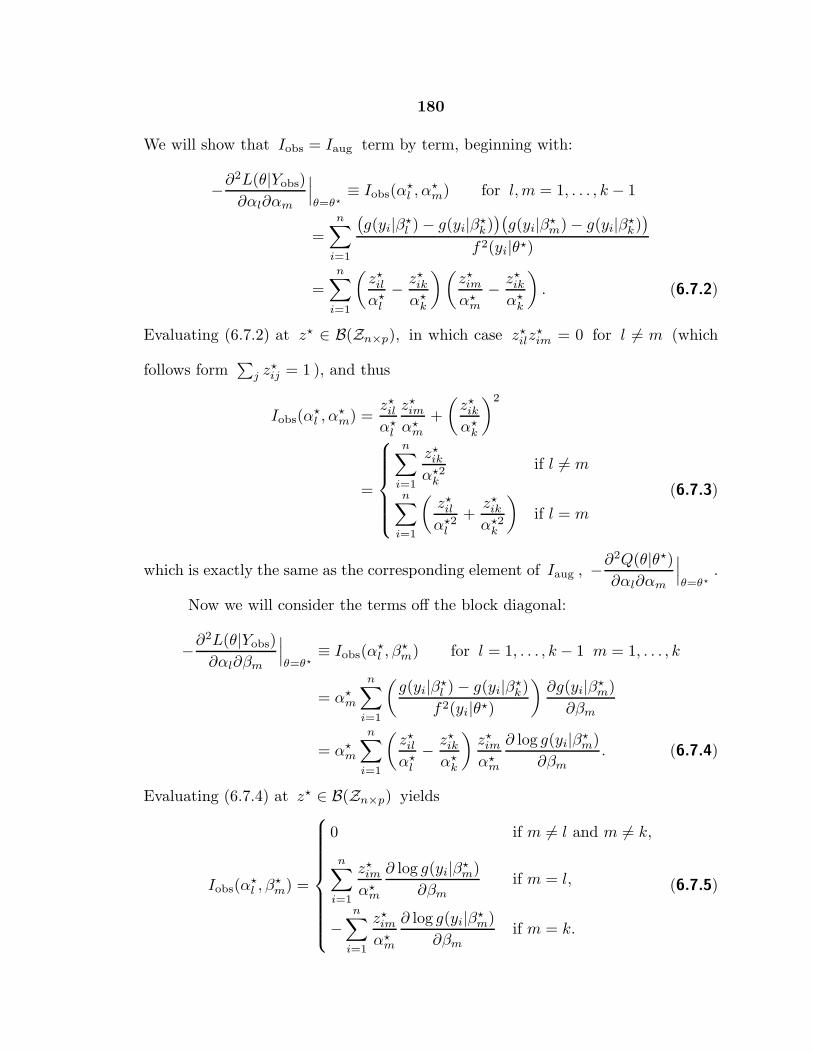
180

We will show that Iobs = Iaug term by term, beginning with:

−∂2L(θ|Yobs)

∂αl∂αm

∣∣∣θ=θ⋆

≡ Iobs(α⋆l , α

⋆m) for l,m = 1, . . . , k − 1

=

n∑

i=1

(g(yi|β⋆

l ) − g(yi|β⋆k))(g(yi|β⋆

m) − g(yi|β⋆k))

f2(yi|θ⋆)

=

n∑

i=1

(z⋆il

α⋆l

− z⋆ik

α⋆k

)(z⋆im

α⋆m

− z⋆ik

α⋆k

). (6.7.2)

Evaluating (6.7.2) at z⋆ ∈ B(Zn×p), in which case z⋆ilz

⋆im = 0 for l 6= m (which

follows form∑

j z⋆ij = 1 ), and thus

Iobs(α⋆l , α

⋆m) =

z⋆il

α⋆l

z⋆im

α⋆m

+

(z⋆ik

α⋆k

)2

=

n∑

i=1

z⋆ik

α⋆2k

if l 6= m

n∑

i=1

(z⋆il

α⋆2l

+z⋆ik

α⋆2k

)if l = m

(6.7.3)

which is exactly the same as the corresponding element of Iaug , −∂2Q(θ|θ⋆)

∂αl∂αm

∣∣∣θ=θ⋆

.

Now we will consider the terms off the block diagonal:

−∂2L(θ|Yobs)

∂αl∂βm

∣∣∣θ=θ⋆

≡ Iobs(α⋆l , β

⋆m) for l = 1, . . . , k − 1 m = 1, . . . , k

= α⋆m

n∑

i=1

(g(yi|β⋆

l ) − g(yi|β⋆k)

f2(yi|θ⋆)

)∂g(yi|β⋆

m)

∂βm

= α⋆m

n∑

i=1

(z⋆il

α⋆l

− z⋆ik

α⋆k

)z⋆im

α⋆m

∂ log g(yi|β⋆m)

∂βm. (6.7.4)

Evaluating (6.7.4) at z⋆ ∈ B(Zn×p) yields

Iobs(α⋆l , β

⋆m) =

0 if m 6= l and m 6= k,

n∑

i=1

z⋆im

α⋆m

∂ log g(yi|β⋆m)

∂βmif m = l,

−n∑

i=1

z⋆im

α⋆m

∂ log g(yi|β⋆m)

∂βmif m = k.

(6.7.5)

181

But Iobs(α⋆l , β

⋆m) = 0 when m = l or m = k as well since (6.7.5) is the observed

data normal equation for βm . Thus, again Iobs(α⋆l , β

⋆m) = 0 agrees with the the

corresponding Iaug(α⋆l , β

⋆m) , which is zero.

Next we turn to β and first consider l 6= m ,

−∂2L(θ|Yobs)

∂βl∂βm

∣∣∣θ=θ⋆

≡ Iobs(β⋆l , β

⋆m) for l,m = 1, . . . , k

=n∑

i=1

α⋆l α

⋆m

∂∂βl

g(yi|βl)∂

∂βmg(yi|βm)

f2(yi|θ⋆)

=

n∑

i=1

α⋆l α

⋆mz

⋆ilz

⋆im

∂ log g(yi|β⋆l )

∂βl

∂ log g(yi|β⋆m)

∂βm,

which is zero at z⋆ ∈ B(Zn×p) since l 6= m , again agreeing with Iaug(β⋆l , β

⋆m) .

Finally, we consider l = m ,

−∂2L(θ|Yobs)

∂βl∂βl

∣∣∣θ=θ⋆

≡ Iobs(β⋆l , β

⋆l )

=

n∑

i=1

α⋆2

l

(∂

∂βlg(yi|βl)

f(yi|θ⋆)

)2

− α⋆l

∂2

∂β2l

g(yi|β⋆l )

f(yi|θ⋆)

=

n∑

i=1

z⋆2

il

(∂ log g(yi|β⋆

l )

∂βl

)2

− z⋆il

∂2

∂β2l

g(yi|β⋆l )

g(yi|θ⋆l )

,

Once again, after noting that z⋆ij = z⋆2

ij , when z⋆ ∈ B(Zn×p) the expression agrees

with Iaug(β⋆l , β

⋆m) , which completes the proof.

Proof of Proposition 2: Without loss of generality, we assume the last row of

z⋆ is identical to the j th row of z⋆ , where j 6= k . Clearly α⋆j = α⋆

k , since

182

α⋆j =

∑i z

⋆ij/n . This fact along with (6.2.2) gives us

z⋆ij

α⋆j

=z⋆ik

α⋆k

for i = 1, . . . , n.

Thus, Iobs(α⋆j , ξ

⋆) = 0 , where ξ is any component of θ (see (6.7.2) and (6.7.4)).

6.7.2. Large-sample behavior of kr – preliminary theoretical results

Figure 6.2 gives evidence that rn(k|k0) → r(k|k0) . In this section we use this propo-

sition along with a second proposition to show that with probability one the limit

supremum of kr will be no larger than k0 , thus confirming the non-overestimation

that we observed in the previous sections. After we present Theorem 6.2, we will

discuss how the two new propositions, (P3) and (P4), might be proven.

Theorem 6.2: Suppose

(P3) limn→∞ rn(k|k0) = r(k|k0) , almost surely for any k ≥ k0

(P4) If k > k0 then r(k|k0) > r(k0|k0) .

Then if k0 ≥ 2 ,

lim supn→∞

kn ≤ k0, a.s.

Proof: For any k > k0 , from (P3) and (P4) we have,

P

[∞⋂

m=1

∞⋃

n=m

{rn(k|k0) ≤ rn(k0|k0)}]

= 0. (6.7.6)

Since k takes on only countably many values, (6.7.6) implies

P

[∞⋃

k=k0+1

∞⋂

m=1

∞⋃

n=m

{rn(k|k0) ≤ rn(k0|k0)}]

= 0. (6.7.7)

183

By the definition of kn , we have

{kn = k} ⊂ {rn(k|k0) ≤ rn(k0|k0)},

and thus (6.7.7) implies

P

[∞⋃

k=k0+1

∞⋂

m=1

∞⋃

n=m

{kn = k}]

= 0.

Now it remains to discuss propositions 3 and 4, the first of which is more of a

regularity condition.

Proposition 3: If Yobs = (y1, y2, . . . , yn) consists of independent observations from

(6.1.1) with k0 components, then

limn→∞

rn(k|k0) ≡ r(k|k0) exists almost surely.

In order to prove Proposition 3, by (6.4.3) of Theorem 6.3, it suffices to show that

with probability 1,

limn→∞

supu6=0

limǫ→0

R(θ⋆k + ǫu|Yobs) = lim

n→∞supu6=0

{u⊤Imis(n)u

u⊤Iaug(n)u

}= sup

u6=0lim

n→∞

{u⊤Imis(n)u

u⊤Iaug(n)u

}

exists. If θ⋆k is consistent, we should be able to prove this without too much

difficulty. The technical difficulty here involves dealing with the possibility that

Iaug may be ill-behaved when θ⋆k converges to a boundary value of Θk . This

problem will be the subject of future work. The next proposition will likely prove

to be even more challenging.

Proposition 4: If k > k0 , then r(k|k0) > r(k0|k0) .

184

This proposition is at the heart of Theorem 6.2 and its proof has many subtleties.

For the moment we will prove a related result that we hope will ultimately lead to

Proposition 4.

Proposition 4 ′ : Let k > k0 and θk = (θk0, ξ) , where ξ are the additional

parameters the model f(y|θk) has compared with f(y|θk0) . Then

rn(k|k0) ≥ r′n(k0|k0, ξ = ξ⋆),

where r′n(k0|k0, ξ = ξ⋆) is the rate of convergence of the EM algorithm that cal-

culates θ⋆k0

conditional on ξ = ξ⋆ , where θ⋆k = (θ⋆

k0, ξ⋆) is the MLE of θk from

fitting f(y|θk) .

Proof: This result can be seen from (6.4.3):

rn(k|k0) = supu6=0

{u⊤Imisu

u⊤Iaugu

}≥ sup

u6=0,u∈U

{u⊤Imisu

u⊤Iaugu

}= r′n(k0|k0, ξ = ξ⋆),

where U is a subspace of Rd with all elements corresponding to ξ equal to zero.

The relevance of Proposition 4 ′ to Proposition 4 lies in showing

limn→∞

r′n(k0|k0, ξ = ξ⋆) = r′(k0|k0, ξ = 0),

the final term of which is r(k0|k0) ( limn→∞ rn(k|k0) = r(k|k0) is guaranteed by

Proposition 3). The reason that we can expect this to be true is as follows. If

we fit a model with k ≥ k0 , the true model is contained in the subspace Θ0 of

Θk , where θk has αj = 0 for j ≥ k0 + 1 . If maximum likelihood estimates are

consistent, then θ⋆k will converge to a value in Θ0 . Thus, the conditional EM

185

algorithm with model f(Yobs|θk) should converge at the same rate, asymptotically

as the unconditional EM algorithm with model f(Yobs|θk0) . We must be cautious,

however, since Θ0 is contained in the boundary of Θk and thus the standard

consistency arguments need to be carefully checked. Even more important, (6.4.3)

assumes that ∇L(θk|Yobs) = 0 at θk = θ⋆k . However, the fact that θ⋆

k converges

to a boundary point of Θk implies that this condition might not hold, a possibility

that will complicate the theoretical derivation here.

References

Aitkin, M., Anderson, D. and Hinde, J. (1981). Statistical modeling of data on

teaching styles. J. R. Statist. Soc. A, 144, 419-461.

Aitkin, M., and Rubin, D. B. (1985). Estimation and hypothesis testing in finite

mixture models. J. R. Statist. Soc. B, 47 67-75.

Amemiya, T. (1984). Tobit models: a survey. J. Econometrics 24, 3-61.

Amit, Y. and Grenander, U. (1991). Comparing sweep strategies for stochastic

relaxation. J. of Multivariate Analysis. 37, 197-222.

Beaton, A. E. (1964). The use of special matrix operations in statistical calculus.

Education Testing Service Research Bulletin, RB-64-51.

Bishop, Y. M. M., Fienberg, S. E. and Holland, P. W. (1975). Discrete Multivariate

Analysis: Theory and Practice. MIT Press, Cambridge, Massachusetts.

Carnahan, B., Luther, H. A. and Wilkes, J. O. (1969). Applied Numerical Methods.

John Wiley & Sons, New York.

Dempster, A. P., Laird, N. M. and Rubin, D. B. (1977). Maximum likelihood

estimation from incomplete-data via the EM algorithm (with discussion).

J. R. Statist. Soc. B, 39, 1-38.

Dempster, A. P., Laird, N. M. and Rubin, D. B. (1980). Iteratively reweighted

least squares for linear regression when errors are normal/independent dis-

tributed. Multivariate Analysis V, 35-37.

Dyk, D. A. van (1993). Fitting log-linear models to contingency tables with incom-

plete data. Technical Report 381, Department of Statistics, University of

Chicago.

186

187

Dyk, D. A. van and Meng, X. L. (1994). Permuting CM steps within the ECM

algorithm: implementational strategies and cautions. Technical Report 397,

Department of Statistics, University of Chicago. Submitted to J. Computat.

Graph. Statist.

Dyk, D. A. van, Meng, X. L. and Rubin, D. B. (1994). Maximum likelihood estima-

tion via the ECM algorithm: computing the asymptotic variance. Technical

Report 380. Dept. of Statistics, University of Chicago.

Dyk, D. A. van, Meng, X. L. and Rubin, D. B. (1995). Maximum likelihood estima-

tion via the ECM algorithm: computing the asymptotic variance. Statistica

Sinica 5, 55-75.

Fessler, J. A. and Hero, A. O. (1994). Space-alternating generalized expectation-

maximization algorithm. IEEE Tran. on Signal Processing 42 2664-77.

Henna, J. (1985). On estimation of countable mixtures of continuous distributions.

J. of the Japan. Statist. Soc. 15, 75-82.

Horn, R. A. and Johnson, C. R. (1985). Matrix Analysis. Cambridge University

Press, New York.

Jamshidian, M. and Jennrich, R. I. (1993). Conjugate gradient acceleration of the

EM algorithm. J. Am. Statist. Assoc. 88, 221-228.

Kayalar, S. and Weinert, H. L. (1988). Error bounds for the method of alternating

projections. Math. Control Signals Systems 1, 43-59.

Kent, J. T. and Tyler, D. E. (1991). Redescending M-estimates of multivariate

location and scatter. Ann. Statist. 19, 2102-2119.

Kent, J. T., Tyler, D. E. and Vardi, Y. (1994). A curious likelihood identity for the

multivariate t-distribution. Commun. Statist. – Simula. 23, 441-453.

188

Laird, N., Lange, N. and Stram, D. (1987). Maximizing likelihood computations

with repeated measures: application of the EM algorithm. J. Am. Statist.

Assoc. 82, 97-105.

Laird, N. M. and Ware, J. H. (1982). Random effects models for longitudinal data.

Biometrics 38, 967-74.

Lange, K. (1995). A quasi-Newtonian acceleration of the EM algorithm. Statistica

Sinica 5, 1-18.

Lange K., Little, R. J. A. and Taylor, J. M. G. (1989). Robust statistical modeling

using the t-distribution. J. Am. Statist. Assoc. 84, 881-896.

Lansyk, D. and Casella, G. (1990). Improving the EM algorithm. Computing

Science and Statistics: Proceedings of the Symposium on the Interface, 420-

424.

Lindstrom, M. J. and Bates, D. M. (1988). Newton-Raphson and EM algorithms

for linear mixed-effects models for repeated-measure data. J. Am. Statist.

Assoc. 83, 1014-1022.

Little, R. J. A. (1988). Robust estimation of the mean and covariance matrix from

data with missing values. Applied Statistics, 37, 23-39.

Little, R. J. A. and Rubin, D. B. (1987). Statistical Analysis with Missing Data.

John Wiley & Sons, New York.

Liu, C. and Rubin, D. B. (1995a). The ECME algorithm: a simple extension of EM

and ECM with fast monotone convergence. Biometrika, 81, 633-48.

Liu, C. and Rubin, D. B. (1995b). ML estimation of the t-distribution using EM

and its extensions, ECM and ECME. Statistica Sinica, 5, 19-40.

Louis, T. A., (1982). Finding the observed information matrix when using the EM

algorithm. J. R. Statist. Soc. B, 44, 226-233.

189

Maine, M., Boullion, T. and Rizzuto, G. T. (1991). Detecting the number of com-

ponents in a finite mixture having normal components. Commun. Statist.

–Theory Meth. 20, 611-620.

Mardia, K. V., Kent, J. T. and Bibby, J. M. (1979). Multivariate Analysis. Aca-

demic Press, London.

Meng, X. L. (1990). Towards complete results for some incomplete-data Problems.

Ph.D. Thesis, Harvard University, Department of Statistics.

Meng, X. L. (1994). On the rate of convergence of the ECM algorithm. Ann.

Statist. 22, 326-339.

Meng, X. L. and Pedlow, S. (1992). EM: A bibliographic review with missing

articles. Proc. Statist. Comp. Sect., 24-27. Washington, D.C.: American

Statistical Association.

Meng, X. L. and Rubin, D. B. (1991a). Using EM to obtain asymptotic variance-

covariance matrices: the SEM algorithm. J. Am. Statist. Assoc. 86,

899-909.

Meng, X. L. and Rubin, D. B. (1991b). IPF for contingency tables with missing data

via the ECM algorithm. Proc. Statist. Comp. Sect., 244-247. Washington,

D.C.: American Statistical Association.

Meng, X. L. and Rubin, D. B. (1992). Recent extensions to the EM algorithm (with

discussion). In Bayesian Statistics 4, Ed. J. M. Bernardo, J. O. Berger, A.

P. Dawid and A. F. M. Smith, pp. 307-20. Oxford University Press.

Meng, X. L. and Rubin, D. B. (1993). Maximum likelihood estimation via the ECM

algorithm: a general framework. Biometrika 80, 267-78.

Meng, X. L. and Rubin, D. B. (1994a). On the global and componentwise rates

of convergence of the EM algorithm. Linear Algebra and its Applications

(Special issue honoring Ingram Olkin) 199, 413-425.

190

Meng, X. L. and Rubin, D. B. (1994b). Efficient methods for estimating and testing

with seemingly unrelated regressions in the presence of latent variables and

missing data. To appear in a special volume in honor of Arnold Zellner.

Orchard, T. and Woodbury, M. A. (1972). A missing information principle theory

and application. Proceedings of the 6th Berkeley Symposium on Mathemat-

ical Statistics and Probability 1, 697-715.

Ortega, J. M. and Rheinboldt, W. C. (1970). Iterative Solutions of Nonlinear

Equations in Several Variables. Academic Press, New York.

Pearson, K. (1894). Contribution to the mathematical theory of evolution. Phil.

Trans. Roy. Soc. A, 185, 71-110.

Rubin, D. B. (1976). Inference and missing data. Biometrika 63, 581-592.

Rubin, D. B. (1983). Iteratively reweighted least squares, Encyclopedia of the Sta-

tistical Sciences, Vol. 4. John Wiley & Sons, New York, pp. 272-275.

Segal, M. R., Bacchetti, P., and Jewell, N. P. (1994). Variances for maximum

penalized likelihood estimates obtained via the EM algorithm. J. R. Statist.

Soc. B, 56, 345-352.

Titterington, D. M., Smith A. F. M. and Markov U. E. (1985). Statistical Analysis

of Finite Mixture Distributions. John Wiley & Sons, New York.

Wei, C. G. and Tanner, M. A. (1990). A monte carlo implementation of the EM al-

gorithm and the poor man’s data augmentation algorithms. J. Am. Statist.

Assoc. 85, 699-704.

Windham, M. P. and Cutler, A. (1992). Information ratios for validating mixture

analyses. J. Am. Statist. Assoc. 87, 1188-1192.

Wolfe, J. H. (1970). Pattern clustering by multivariate mixture analysis. Multivar.

Behav. Res., 5, 329-350.

191

Wu, C. F. J. (1983). On the convergence properties of the EM algorithm. Ann.

Statist. 11, 95-103.

Zangwill, W. (1969). Nonlinear Programming – A Unified Approach. Prentice-Hall,

Englewood Cliffs, New Jersey.

Zellner, A. (1962). An efficient method of estimating seemingly unrelated regres-

sions and tests for aggregation bias. J. Am. Statist. Assoc. 57, 348-368.