The Uncertain Unit Root in Real GNP: Comment

By FRANCIS X. DIEBOLD AND ABDELHAK S. SENHADJI *

Fifteen years after the seminal work of Charles R. Nelson and Charles I. Plosser ( 1982), the question of deterministic vs. sto- chastic trend in U.S. GNP (and other key aggregates) remains open. The surrounding controversy certainly is not due to lack of pro- fessional interest-the literature on the ques- tion is huge. Instead, the low power of tests of stochastic trend (or "difference stationar- ity" in the parlance of John H. Cochrane [1988]) against nearby deterministic-trend ("trend-stationary") alternatives, together with the fact that such nearby alternatives are the relevant ones, explains the lack of consensus.

In an important paper, Glenn D. Rudebusch (1993) contributes to the "we don't know" literature initiated by Lawrence J. Christiano and Martin Eichenbaum (1990) by arguing that unit-root tests applied to U.S. quar- terly real GNP per capita lack power even against distant alternatives. First, Rudebusch shows that the best-fitting trend-stationary and difference-stationary models imply very different medium- and long-run dynamics. Then he shows with an innovative procedure that, regardless of which of the two models obtains, the exact finite-sample distributions of the Dickey-Fuller test statistics are very similar. Thus, Rudebusch concludes that unit-root tests are unlikely to be capable of discriminating between deterministic and stochastic trends.

The distinction between trend stationarity is not critical in some contexts. Often, for example, one wants a broad gauge of the persistence in aggregate output dynamics, in which case one may be better informed by an interval estimate of the dominant root in an autoregressive approximation. Hence the importance of James H. Stock's (1991) clever procedure for computing such intervals. But the distinction between trend stationarity and difference stationarity is potentially im- portant in other contexts, such as economic forecasting, because the trend- and difference- stationary models may imply very different dynamics and hence different point forecasts, as argued by Stock and Mark W. Watson (1988) and John Y. Campbell and Pierre Perron (1991) .

Motivated by the potential importance of unit roots for the forecasting of aggregate output, as well as other considerations that we discuss later, we extend Rudebusch's (1993) analysis to sev- eral long spans of annual U.S. real GNP data, and we examine the robustness of all results to variations in the sample period and the particular GNP measure employed. As we shall show, the outcome is both surprising and robust.

I. Construction of Annual U.S. Real GNP Series, 1869-1993

Three annual "raw" data series underlie the annual series used in this paper. We create the first two, which are real GNP series, by splic- ing the 1869-1929 real GNP series of Nathan S. Balke and Robert J. Gordon (1989) or Christina D. Romer (1989) to the 1929-1993 real GNP series reported in table 1.10 of the National Income and Product Accounts of the United States, measured in billions of 1987 dollars. The two historical real GNP series are measured in billions of 1982 dollars, which we convert to 1987 dollars by multi- plying by 1.166, which is the ratio of the 1987 dollar value to the 1982 dollar value in the overlap year 1929, at which time the

* Diebold: Department of Economics, University of Pennsylvania, 3718 Locust Walk, Philadelphia, PA 19104-6297, and NBER; Senhadji: Olin School of Business, Washington University, One Brookings Drive, St. Louis, MO 63130-4899. For constructive and insightful comments we thank Craig Hakkio, Andy Postlewaite, Glenn Rudebusch, Chuck Whiteman, and two referees, as well as numerous seminar participants, but all errors remain ours alone. We gratefully ac- knowledge support from the National Science Foun- dation, the Sloan Foundation, and the University of Pennsylvania Research Foundation.

1291

1292 THE AMERICAN ECONOMIC REVIEW DECEMBER 1996

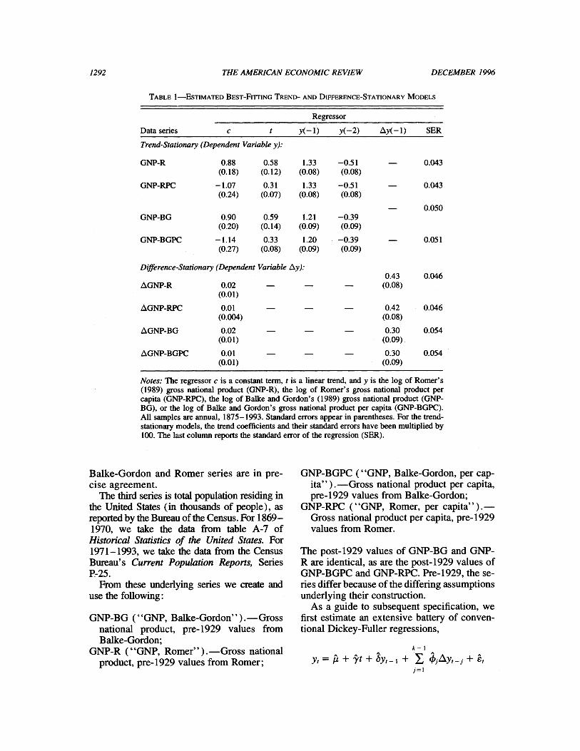
TABLE 1-ESTIMATED BEST-FITrING TREND- AND DIFFERENCE-STATIONARY MODELS

Regressor Data series c t y(-1) y(-2) Ay(-l) SER

Trend-Stationary (Dependent Variable y):

GNP-R 0.88 0.58 1.33 -0.51 - 0.043 (0.18) (0.12) (0.08) (0.08)

GNP-RPC -1.07 0.31 1.33 -0.51 - 0.043 (0.24) (0.07) (0.08) (0.08)

- 0.050 GNP-BG 0.90 0.59 1.21 -0.39

(0.20) (0.14) (0.09) (0.09) GNP-BGPC -1.14 0.33 1.20 -0.39 - 0.051

(0.27) (0.08) (0.09) (0.09)

Difference-Stationary (Dependent Variable Ay): 0.43 0.046

AGNP-R 0.02 - (0.08) (0.01)

AGNP-RPC 0.01 - 0.42 0.046 (0.004) (0.08)

AGNP-BG 0.02 0.30 0.054 (0.01) (0.09)

AGNP-BGPC 0.01 - 0.30 0.054 (0.01) (0.09)

Notes: The regressor c is a constant term, t is a linear trend, and y is the log of Romer's (1989) gross national product (GNP-R), the log of Romer's gross national product per capita (GNP-RPC), the log of Balke and Gordon's (1989) gross national product (GNP- BG), or the log of Balke and Gordon's gross national product per capita (GNP-BGPC). All samples are annual, 1875-1993. Standard errors appear in parentheses. For the trend- stationary models, the trend coefficients and their standard errors have been multiplied by 100. The last column reports the standard error of the regression (SER).

Balke-Gordon and Romer series are in pre- cise agreement.

The third series is total population residing in the United States (in thousands of people), as reported by the Bureau of the Census. For 1869- 1970, we take the data from table A-7 of Historical Statistics of the United States. For 1971-1993, we take the data from the Census Bureau's Current Population Reports, Series P-25.

From these underlying series we create and use the following:

GNP-BG ("GNP, Balke-Gordon").-Gross national product, pre-1929 values from Balke-Gordon;

GNP-R ("GNP, Romer" ).-Gross national product, pre-1929 values from Romer;

GNP-BGPC ("GNP, Balke-Gordon, per cap- ita" ) .-Gross national product per capita, pre-1929 values from Balke-Gordon;

GNP-RPC ("GNP, Romer, per capita" ). Gross national product per capita, pre-1929 values from Romer.

The post-1929 values of GNP-BG and GNP- R are identical, as are the post-1929 values of GNP-BGPC and GNP-RPC. Pre-1929, the se- ries differ because of the differing assumptions underlying their construction.

As a guide to subsequent specification, we first estimate an extensive battery of conven- tional Dickey-Fuller regressions,

k-I

YtA + et + sY, _M+ '

Ayi+ j=1

VOL. 86 NO. 5 DIEBOLD AND SENHADJI: UNCERTAIN ROOT IN GNP, COMMENT 1293

-3.5

4.0 Trend-Stationary -

Forecast

-45.0

sol0 Historical GNP sf X r Per'tCapia

GN ff-6werence-StatIonary -5.5 Per Capita - ' Forecast

-5.5.

-8.0.

-8.5. 1880 1900 1920 194 1980 198.

FIGURE 1. GNP PER CAPITA, HISTORICAL AND Two FORECASTS

Notes: We plot U.S. real GNP per capita, together with the optimal 1934-1993 forecasts (made in 1933) from the best-fitting trend-stationary model (short-dashed line) and from the best-fitting difference-stationary model (long-dashed line). Pre-1929 GNP data are from Romer (1989).

for each of the four real GNP variables discussed above and for k = 1 through k = 6.' A unit root corresponds to 6 = 1, and the Dickey-Fuller sta- tistic is Ir = ( - 1)/SE(s), where SE(S) is the standard error of the estimated coefficient, S. The common sample period for all variables and for all values of k is 1875-1993. The se- lected lag order in the Dickey-Fuller regression for all four variables is k = 2, regardless of whether we used the Schwarz criterion, the Akaike criterion, or conventional hypothesis- testing procedures to determine k. More pre- cisely, all diagnostics indicate that k = 1 is grossly inadequate and that k > 2 is unnecessary and therefore wasteful of degrees of freedom.

TABLE 2-EXACT p VALUES OF THE DICKEY-FULLER STATISTIC

p value

Dataseries k = 2 k = 3 k = 4 -

GNP-R Pr[U s rsample IfTs(,)] 0.625 0.690 0.592 PrU[ s isample IfDS(i')] 0.001 0.005 0.012

GNP-RPC PrU s sampe If TS()] 0.668 0.673 0.695 Pr[U s '..mpi. IfDS(')] 0.001 0.007 0.017

GNP-BG Pr[, ' .sampIe IfTS(f)] 0.651 0.616 0.657 PrU[ s .sampie IfDS(^)] 0.005 0.002 0.020

GNP-BGPC Pr[u s ,sampIe IfTS(7)] 0.692 0.656 0.711 Pr[ s .sapie IfDS(7)] 0.006 0.003 0.021

Notes: The Dickey-Fuller statistic is represented by 5r; fTs(5-) is the empirical distribution of 5- conditional on the trend-stationary model, fDs(5r) is the empirical dis- tribution of 5- conditional on the difference-stationary model, k is the augmentation lag order in the Dickey- Fuller regression, and Pr[5- s Tf.Lfms(f)] and Pr4 5 s -sarnpleIf D5(5)] are the probabilities of obtaining 5 s 5-smpI.

under the trend-stationary and the difference-stationary models. The variables are the log of Romer's (1989) gross national product (GNP-R), the log of Romer's gross national product per capita (GNP-RPC), the log of Balke and Gordon's (1989) gross national product (GNP-BG), or the log of Balke and Gordon's gross na- tional product per capita (GNP-BGPC). All samples are annual, 1875-1993.

Thus, in terms of a "reasonable range" in which to vary k, we focus throughout the paper on k = 2 through k = 4, and .our attention centers on k = 2.

II. Evidence From Rudebusch's Exact Finite-Sample Procedure

We use Rudebusch's ( 1993) procedure throughout. In Table 1 we display the full- sample estimates of the selected trend-stationary and difference-stationary models for each of the four GNP series. For each series, the two models fit equally well, but they imply very different dynamics. This can be seen by com- paring the forecasts shown in Figure 1, in which we show GNP per capita using Romer's ( 1989) pre-1929 values (GNP-RPC) for 1869-1933, followed by the forecasts from

'We gave particular care to the determnination of k, the augmentation lag order, because it is well known that the results of unit-root analyses may vary with k. A number of authors have recently addressed this important problem, ex- ploring the properties of various lag-order selection criteria. For example, Alastair Hall (1994) establishes conditions under which the Dickey-Fuller test statistic converges to the Dickey-Fuller distribution when data-based procedures are used to select k, and he verifies that the conditions are sat- isfied by the popular Schwarz information criterion. Serena Ng and Perron ( 1995), however, argue that t and F tests on the augmentation lag coefficients in the Dickey-Fuller re- gression are preferable, because they lead to less size dis- tortion and comparable power.

1294 THE AMERICAN ECONOMIC REVIEW DECEMBER 1996

0.15

0.12-

0.09 Trend- i Difference-

Stationary Stationary

0.06 -

0.03-

0.00 -7.85 -6.91 -5.97 -5.04 -4.10 -3.16 -2.22 -1.29 -0.35 0.59 1.52

Tsample T

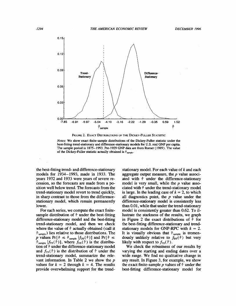
FIGURE 2. EXACT DISTRIBUTIONS OF THE DICKEY-FULLER STATISTIC

Notes: We show exact finite-sample distributions of the Dickey-Fuller statistic under the best-fitting trend-stationary and difference-stationary models for U.S. real GNP per capita. The sample period is 1875-1993. Pre-1929 GNP data are from Romer (1989). The value of the Dickey-Fuller statistic actually obtained is 'sampIe-

the best-fitting trend- and difference-stationary models for 1934-1993, made in 1933. The years 1932 and 1933 were years of severe re- cession, so the forecasts are made from a po- sition well below trend. The forecasts from the trend-stationary model revert to trend quickly, in sharp contrast to those from the difference- stationary model, which remain permanently lower.

For each series, we compute the exact finite- sample distribution of r under the best-fitting difference-stationary model and the best-fitting trend-stationary model, and then we check where the value of r actually obtained (call it Tsample) lies relative to those distributions. The p values Pr[I [ sample IfDs(')] and Pr[^ Tsample IfTs(')], where fDs(') is the distribu- tion of r under the difference-stationary model and fTs('r) is the distribution of r under the trend-stationary model, summarize the rele- vant information. In Table 2 we show the p values for k = 2 through k = 4. The results provide overwhelming support for the trend-

stationary model. For each value of k and each aggregate output measure, the p value associ- ated with r under the difference-stationary model is very small, while the p value asso- ciated with -r under the trend-stationary model is large. In the leading case of k = 2, to which all diagnostics point, the p value under the difference-stationary model is consistently less than 0.01, while that under the trend-stationary model is consistently greater than 0.62. To il- lustrate the starkness of the results, we graph in Figure 2 the exact distributions of r for the best-fitting difference-stationary and trend- stationary models for GNP-RPC with k = 2. It is visually obvious that Tsample is tremen- dously unlikely relative to fDs( 'r) but very likely with respect to fTs( ^).

We check the robustness of our results by varying the starting and ending dates over a wide range. We find no qualitative change in any result. In Figure 3, for example, we show the exact finite-sample p values of r under the best-fitting difference-stationary model for

VOL. 86 NO. 5 DIEBOLD AND SENHADJI: UNCERTAIN ROOT IN GNP, COMMENT 1295

LC)

o_ .

C)

~~~~~- -

Q0S

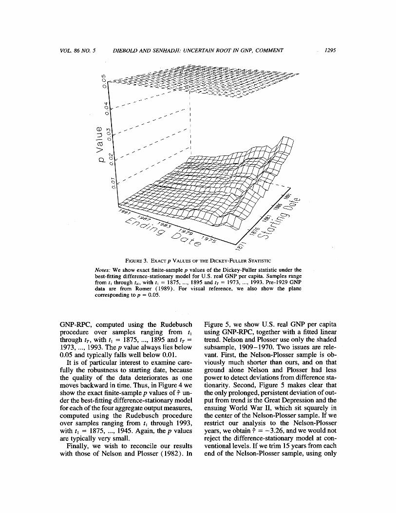
FIG{URE 3. EXACT p VALUES OF THE DICKEY-FULLER STATISTIC

Notes: We show exact finite-sample p values of the Dickey-Fuller statistic under the best-fitting difference-stationary model for U.S. real GNP per capita. Samples range from t, through tN, with t, = 1875, ..., 1895 and tT = 1973,..., 1993. Pre-1929 GNP data are from Romer (1989). For visual reference, we also show the plane corresponding to p = 0.05.

GNP-RPC, computed using the Rudebusch procedure over samples ranging from t1 through tT, with t1 = 1875, ..., 1895 and tT = 1973, ..., 1993. The p value always lies below 0.05 and typically falls well below 0.01.

It is of particular interest to examine care- fully the robustness to starting date, because the quality of the data deteriorates as one moves backward in time. Thus, in Figure 4 we show the exact finite-sample p values of r un- der the best-fitting difference-stationary model for each of the four aggregate output measures, computed using the Rudebusch procedure over samples ranging from t1 through 1993, with t1 = 1875, ..., 1945. Again, the p values are typically very small.

Finally, we wish to reconcile our results with those of Nelson and Plosser (1982). In

Figure 5, we show U.S. real GNP per capita using GNP-RPC, together with a fitted linear trend. Nelson and Plosser use only the shaded subsample, 1909-1970. Two issues are rele- vant. First, the Nelson-Plosser sample is ob-_ viously much shorter than ours, and on that ground alone Nelson and Plosser had less power to detect deviations from difference sta- tionarity. Second, Figure 5 makes clear that the only prolonged, persistent deviation of out- put from trend isi the Great Depression and the ensuing World War II, which sit squarely in the center of the Nelson-Plosser sample. If we restrict our analysis to the Nelson-Plosser years, we obtain r = -3.26, and we would not reject the difference-stationary model at con- ventional levels. If we trim 15 years from each end of the Nelson-Plosser sample, using only

1296 THE AMERICAN ECONOMIC REVIEW DECEMBER 1996

GNP-R 0.04

ai) :3

> 0.02 -

0.00 1870 1880 1890 1900 1910 1920 1930 1940 1950

GNP-RPC 0.04

> 0.02

0.00 1870 1880 1890 1900 1910 1920 1930 1940 1950

GNP-BG 0.04

>Q 0.02

0.00 1870 1880 1890 1900 1910 1920 1930 1940 1950

GNP-BGPC 0.04

> 0.02 -

0.00 1870 1880 1890 1900 1910 1920 1930 1940 1950

Starting Date

FIGURE 4. EXACT P VALUES OF THE DICKEY-FULLER STATISTIC

Notes: We show exact finite-sample p values of the Dickey-Fuller statistic under the best-fitting difference-stationary model for the log of Romer's (1989) gross national product (GNP-R), the log of Romer's gross national product per capita (GNP-RPC), the log of Balke and Gordon's (1989) gross national product (GNP-BG), and the log of Balke and Gordon's gross national product per capita (GNP-BGPC). Samples range from t, through 1993, with t, = 1875,..., 1945. To facilitate comparisons, each subplot is scaled to have a height of 0.05.

VOL. 86 NO. 5 DIEBOLD AND SENHADJI: UNCERTAIN ROOT IN GNP, COMMENT 1297

-3.5-

-4.0- ~ ~ ~ ~ "" 7

1880 1900 i12'0' 1940 190 98

FIGURE 5. GNP PER CAPITA, ACTUAL AND TREND

Notes: We show the log of U.S. real GNP per capita, together with a fitted linear trend. The Nelson and Plosser ( 1982) subsample, 1909- 1970, is shaded. Pre-1929 GNP data are from Romer ( 1989).

1924- 1955, we obtain "r =_ -2.71, corre- sponding to even less evidence against the difference-stationary model. Conversely, as we expand the sample to include years both earlier and later than those used by Nelson and Plosser, the evidence against difference- stationarity grows quickly, because the earlier and later years are highly informative about the question of interest, as output clings tightly to trend. By the time we use the full sample, 1875 - 1993, we obtain "r = -4.57, and we reject difference-stationarity at any reasonable level.

III. Concluding Remarks

There is no doubt that unit-root tests do suffer from low power in many situations of interest. Rudebusch's (1993) analysis of postwar U.S. quarterly GNP illustrates that point starkly. We have shown, however, that Rudebusch' s procedure produces evidence that distinctly favors trend-stationarity using long spans of annual data. Moreover, allow- ing for breaking trend in the spirit of Perron (1989) would only strengthen our results. Thus, the U.S. aggregate output data are not as uninformative as many believe. Interest- ingly, the same conclusion has been reached by very different methods in the Bayesian lit- erature (e.g., David N. DeJong and Charles H. Whiteman, 1991) and in out-of-sample

forecasting competitions (e.g., John Geweke and Richard A. Meese, 1984; DeJong and Whiteman, 1994).

We have already stressed the importance of our results for forecasting aggregate output. They are also important for macroeconometric modeling more generally. For example, recent important work by Graham Elliott ( 1995) points to the nonrobustness of cointegration methods to deviations of variables from difference-stationarity. More precisely, Elliott shows that even very small deviations from difference-stationarity can invalidate the infer- ential procedures associated with conventional cointegration analyses. Our results suggest that U.S. aggregate output is not likely to be difference-stationary: the dominant autoregres- sive root is likely close to, but less than, unity. This points to the desirability of additional work on inference in macroeconometric mod- els with dynamics that are long-memory but mean-reverting, as in Diebold and Rudebusch (1989), or short-memory with roots local to unity, as in Elliott et al. ( 1992).

Finally, let us summarize our contribution as we see it. We do not take issue with Rudebusch; we in fact study very different aggregate output series, and certainly we are not the first to notice that the use of longer GNP samples may produce sharper unit-root inference (see, e.g., Stock and Watson, 1986). Rather, we are skeptical of blanket generalizations of the Christiano- Eichenbaum-Rudebusch results, prevalent in the recent oral tradition. We have argued that, even for the famously recalcitrant aggregate output series, unit-root tests over long spans can be informative, and they may be important for point forecasting, among other things. Our results make clear that uncritical repetition of the "we don't know, and we don't care" man- tra is just as scientifically irresponsible as blind adoption of the view that "all macroeconomic series are difference-stationary," or the view that "all macroeconomic series are trend- stationary." There is simply no substitute for serious, case-by-case, analysis.

REFERENCES

Balke, Nathan S. and Gordon, Robert J. "The Estimation of Prewar Gross National Prod- uct: Methodology and New Evidence."

1298 THE AMERICAN ECONOMIC REVIEW DECEMBER 1996

Journal of Political Economy, February 1989, 97(1), pp. 38-92.

Bureau of the Census, U.S. Department of Com- merce. Historical statistics of the United States. Washington, DC: U.S. Government Printing Office, various years.

. Current population reports, Series P-25. Washington, DC: U.S. Government Printing Office, various years.

Campbell, John Y. and Perron, Pierre. "Pitfalls and Opportunities: What Macroeconomists Should Know About Unit Roots," in Olivier Blanchard and Stanley Fischer, eds., NBER macroeconomics annual, 1991. Cambridge, MA: MIT Press, 1991, pp. 141-201.

Christiano, Lawrence J. and Eichenbaum, Martin. "Unit Roots in Real GNP: Do We Know and Do We Care?" Carnegie-Rochester Conference Series on Public Policy, Spring 1990, 32, pp. 7-61.

Cochrane, John H. "How Big Is the Random Walk in GNP?" Journal of Political Econ- omy, October 1988, 96(5), pp. 893-920.

Dejong, David N. and Whiteman, Charles H. "The Case for Trend-Stationarity Is Stronger Than We Thought." Journal of Applied Econometrics, October-December 1991, 6(4), pp. 413-421.

.__ "The Forecasting Attributes of Trend- and Difference-Stationary Represen- tations for Macroeconomic Time Series." Journal of Forecasting, April 1994, 13, pp. 279-97.

Diebold, Francis X. and Rudebusch, Glenn D. "Long Memory and Persistence in Aggre- gate Output." Journal of Monetary Eco- nomics, September 1989, 24(2), pp. 189-209.

Elliott, Graham. "On the Robustness of Coin- tegration Methods When the Regressors Almost Have Unit Roots." Unpublished manuscript, Department of Economics, Uni-

- versity of California, San Diego, 1995. Elliott, Graham; Rothenberg, Thomas J. and

Stock, James H. "Efficient Tests for an Au- toregressive Unit Root." National Bureau of Economic Research (Cambridge, MA) Technical Working Paper No. 130, 1992.

Geweke, John and Meese, Richard A. "A Com- parison of Autoregressive Univariate Fore- casting Procedures for Macroeconomic Time Series." Journal of Business and Eco- nomic Statistics, July 1984, 2(3), pp. 191- 200.

Hall, Alastair. "Testing for a Unit Root in Time Series with Pretest Data-Based Model Se- lection." Journal of Business and Eco- nomic Statistics, October 1994, 12(4), pp. 461-70.

National income and product accounts of the United States. Washington, DC: U.S. De- partment of Commerce, various years.

Nelson, Charles R. and Plosser, Charles I. "Trends and Random Walks in Macro- economic Time Series: Some Evidence and Implications." Journal of Monetary Economics, September 1982, 10(2), pp. 139-62.

Ng, Serena and Perron, Pierre. "Unit Root Tests in ARMA Models with Data-Dependent Methods for the Selection of the Truncation Lag." Joumal of the American Statistical Association, March 1995, 90(429), pp. 268-81.

Perron, Pierre. "The Great Crash, the Oil Price Shock, and the Unit Root Hypothesis." Econometrica, November 1989, 57(6), pp. 1361- 1401.

Romer, Christina D. "The Prewar Business Cy- cle Reconsidered: New Estimates of Gross National Product, 1869-1908." Journal of Political Economy, February 1989, 97(1), pp. 1-37.

Rudebusch, Glenn D. "The Uncertain Unit Root in Real GNP." American Economic Re- view, March 1993, 83(1), pp. 264-72.

Stock, James H. "Confidence Intervals for the Largest Autoregressive Root in U.S. Mac- roeconomic Time Series." Journal of Mon- etary Economics, December 1991, 28(3), pp. 435-59.

Stock, James H. and Watson, Mark W. "Does GNP Have a Unit Root?" Economics Let- ters, March 1986, 22, pp. 147-51.

. _ "Variable Trends in Economic Time Series." Journal of Economic Perspectives, Summer 1988, 2(3), pp. 147-74.