The UN Global Policy Model (GPM): Technical...
53
The UN Global Policy Model ( GPM ): Technical Description ◊ Francis Cripps and Alex Izurieta * May 2014 ◊ This technical overview refers specifically to version 5.2c of the GPM. * Francis Cripps: Director of Alphametrics Alex Izurieta: Senior Economist, UNCTAD
Transcript of The UN Global Policy Model (GPM): Technical...
The UN Global Policy Model ( GPM ):
Technical Description ◊
Francis Cripps and Alex Izurieta *
May 2014
◊ This technical overview refers specifically to version 5.2c of the GPM.
* Francis Cripps: Director of Alphametrics
Alex Izurieta: Senior Economist, UNCTAD

TABLE OF CONTENTS GPM overview................................................................................................................................ 1 Model structure and specification .......................................................................................... 4 Domestic and global interactions ............................................................................................................................ 4 Finance and stock flow closures ...........................................................................................................................................5 Demographics, labour and income distribution............................................................................................................6
Behavioural equations................................................................................................................ 8 Income and expenditure .............................................................................................................................................. 8 The private sector .......................................................................................................................................................................8 The government sector.............................................................................................................................................................9
Trade and the external current account.............................................................................................................10 Trade in manufactured goods............................................................................................................................................. 10 Trade in services....................................................................................................................................................................... 12 Trade in primary commodities .......................................................................................................................................... 12 Energy trade and environmental considerations ...................................................................................................... 13 External income and transfers ........................................................................................................................................... 15
The financial sector: flow of funds, holding gains and balances .............................................................15 Government debt and asset transactions ...................................................................................................................... 17 The external position and exchange rates..................................................................................................................... 19 The domestic banking system ............................................................................................................................................ 21 Capital stock and private wealth ....................................................................................................................................... 22 Interest rates .............................................................................................................................................................................. 22
Inflation and employment.........................................................................................................................................23 Price formation.......................................................................................................................................................................... 23 Employment................................................................................................................................................................................ 24
Selected multiplier tables........................................................................................................25 Appendix: notation, deflators and model variables ........................................................35 1. Notation and measurement conventions .......................................................................35 Domestic income and expenditure .......................................................................................................................35 International trade and other external transactions....................................................................................35 Prices and rates..............................................................................................................................................................37 Assets and liabilities ....................................................................................................................................................37 Actual and simulated values.....................................................................................................................................39 Residuals and instruments .......................................................................................................................................39
2. Real values, volumes and price deflators......................................................................40 3. Variables and identities ......................................................................................................42 Model variables ..............................................................................................................................................................42 Additional variables for policy evaluation.........................................................................................................49

GPM technical description p. 1
GPM OVERVIEW
The Global Policy Model (GPM) is a tool for investigation of regional and global policy issues. 1 The model may be used to trace historical developments and simulate potential future impacts of trends, shocks and policy initiatives over medium‐term timescales up to 15 or 20 years into the future. The main purpose of the GPM is to provide empirical and rigorously structured insights into problems of policy design and international cooperation. The GPM is not a (short‐term) forecasting model.
In common with other macro‐models, the GPM comprises a databank of historical time series and a set of computer programs that organize the original data, estimate model parameters and generate scenarios. Both systems, the dataset and the model, are self‐contained and distributable. As far as data is concerned, the major challenge is to benefit from the considerable availability of annual data for all countries and compile the various sources in a rigorous manner across fields, countries and time. The GPM enforces strict national accounting consistency, extended into related domains such as trade and balance of payments, banking and government finance, population and employment, income distribution, energy and emissions, etc.
The GPM has been designed to facilitate alternative schemes of geographic disaggregation (flexible geometry) depending on the purposes for which the model is used. A standard decomposition in the current version of the model includes sixteen G20 members and a further nine country groups, amounting to a total of 25 countries and groups covering the world as a whole. Other decompositions have been used to study specific topics, like energy production, use and environmental impact; export diversification and trade agreements, etc.
Regarding the modelling framework, early global empirical investigations of policy issues attempted to ensure consistency by putting together country models provided independently by national governments or think‐tanks. This approach, like that formalised in the LINK project under the auspices of the UN, have known limitations
1 The first version of the GPM was created by the Department of Economic and Social Affairs of the United Nations in 2007. It drew heavily from the experience of more than 30 years of global modelling acquired by the Department of Applied Economics (DAE) of the University of Cambridge, UK. One of the main authors of DAE’s global modelling work, Francis Cripps, has been the principal investigator behind all versions of the UN GPM, including this one (5.c). Francis Cripps was joined by Alex Izurieta while at the University of Cambridge, then DESA and at present UNCTAD, and by Rob Vos, then Director of the Department of Policy Analysis of DESA, with whom earlier presentations of the GPM were co‐authored. Apart from DESA, other partners have collaborated in the development of the model, most notably UNDP’s International Policy Centre (IPC), Cambridge Endowment for Research on Finance (CERF, University of Cambridge), UNCTAD, ILO, and the Global Development and Environment Institute (GDAE) of Tufts University (MA, US). From December 2013 onwards, the responsibility for the maintenance and revisions of the model resides on UNCTAD. UNCTAD is committed to make the databank and model programmes available to a wider audience.

GPM technical description p. 2
due to the diversity of underlying models and the limits of linking outcomes with fixed trade matrices. The GPM breaks with this pattern as it relies on a fully integrated analytical structure where standardized models of countries or country groups are resolved endogenously through a dynamic trade and financial structure. This facilitates the investigation of global interactions and dynamics over time as well as the simultaneous evaluation of policies and outcomes for individual countries with different economic structures and at different levels of development.
Behavioural specification is homogenous across countries and structural differences are explained endogenously within the model rather than being imposed exogenously by the use of different specifications per country. It is not the only model to employ a common specification of behaviour aided by differentiated fixed effects and ‘state’ variables as denominators for correction of heteroskedasticity. In addition, continuing investigation is being undertaken to clarify reasons for differences and relate them to structural variables within the model. For example, if research shows that differences in a particular behaviour reflect different degrees of development, a typical variable to include in the specification is the relative or absolute level of income per capita which itself changes dynamically along the period of a model simulation. Likewise, if differences of behaviour across countries or sectors are attributable to some form of financial constraint, explanatory variables that could be included in the specification are the level of public or private debt, the current account position or the level of international reserves, etc. This ‘structural’ approach opens the door to panel estimation methods which are advantageous when, as in the case of global databanks, there is considerable variation in accuracy of observations for different groups of countries and in different time periods.2
Each variable in the model is specified either by an accounting identity or an econometric specification, while global closure rules and explicit dynamic behaviour ensure model convergence at each point in time. With very limited exceptions, the model is fully endogenous throughout both the historic period and the simulation period.
As in other models, residual terms in behavioural equations over the historical period serve to match 'known' values of the variable being explained.
A more complex task is to generate model values for the period between the last available historical data and the initial period for genuine simulations (typically the ‘next year’). Often such data are well known or can be inferred from partial information or short term forecasts but have not yet reached the international statistical sources used in the model. Thus the GPM ‘aligns’ data for the current year and very recent past
2 Additional information and more robust econometric estimates can be obtained using finer country disaggregations. Some work of this kind has been done for the GPM using 50‐60 countries to include countries with relatively complete historical data and up to 80 countries to include all countries with substantial population or GDP.

GPM technical description p. 3
with estimates obtained from short‐term forecasting models such as DESA’s World Economic Forecasting Model (WEFM), or ILO’s Global Employment Trends (GET), or other sets of assumptions about current developments. This alignment that can be extended one or two years into the future is achieved by target‐instrument algorithms that adjust residuals in behavioural equations to generate the required values of main indicators such as a world oil price index and GDP, inflation, the current account, employment and unemployment in each country.
A ‘plain’ projection further into the outlook period can be generated by assuming future residuals to be nil. Neither such a ‘plain’ projection nor the more informed scenarios explained below have predictive power or probabilities assigned to them. Longer‐term outcomes, being subject to unanticipated turning points, policy changes and shocks, are not knowable in a forecasting sense even though underlying trends in different parts of the world are often persistent. Global fluctuations in trade and investment, exchange rates, stock markets, commodity prices etc. continue to make the policy environment unpredictable and crises such as the 2008‐9 financial meltdown in the USA and Europe can still derail the world economy in unpredictable ways.
Scenarios for the projection period are thought to be conditional upon assumed patterns imputed by adjustment of residuals in the behavioural relations. In other words, they are ‘what if’ scenarios, not forecasts. The baseline is typically thought as a continuation of prevailing policies with slowly decaying residuals but it may also include assumptions about future changes that can be anticipated as probable or highly likely. Alternative projections are typically designed as ‘policy scenarios’ in the broad sense that they embody assumed changes of policy stance that influence behaviour of one equation or a set of equations in a particular manner.
Such policy assumptions can take the form of straightforward ‘add factors’ in say, the government expenditure equation, or the tax equations, or the interest rate equation, etc. Beyond the straightforward modality of constructing ‘what if’’ scenarios by ‘shocks’ in one or a set of variables, the main interest of GPM simulations lies in investigating alternative configurations of policy with different degrees of policy coordination. In the tradition of Jan Tinbergen, such policy schemes are defined using rules in which behaviour of an ‘instrument’ variable is adjusted to aim at achieving a policy ‘target’, often extended in a nuanced manner to examine the potential impact of behavioural changes at a regional or more global level. Complementary to the use of one instrument for each target, a set of additional instruments can be ‘linked’ to contribute together in achieving the targets. For example, it is possible to aim at achieving a target of a particular fiscal budget by taking, say direct taxation alone as an instrument, or by linking changes in direct taxation with a proportional effort made by changes in indirect taxes and government spending. Moreover the GPM allows for conditional activation of policies depending on whether outcomes exceed or fall short of a country's targets. This is important because although global trade and financial markets exert a common influence, the predicament facing individual countries at each point in time varies widely implying that priorities and requirements for policy adjustment that are

GPM technical description p. 4
appropriate for some countries will often be less appropriate or inappropriate for others.
To ensure that model simulations stay within limits of plausibility and have a resonance with historically observed experience, the model can restrict such ‘shocks’ in a way that outcomes of each behavioural variable do not deviate beyond a specified residual distribution. The modeller can explicitly determine the maximum deviation for each variable separately or for the entire model.
Beyond this the extent to which policies can or could have an effective influence on behaviour in each field is evidently a matter for assumption or judgement. This is true enough for government budgets and even more so for 'trade policies', 'industrial policies', 'environmental policies' etc. What the model can test is the potential consequences if targetted policies do have an influence.
MODEL STRUCTURE AND SPECIFICATION
Domestic and global interactions
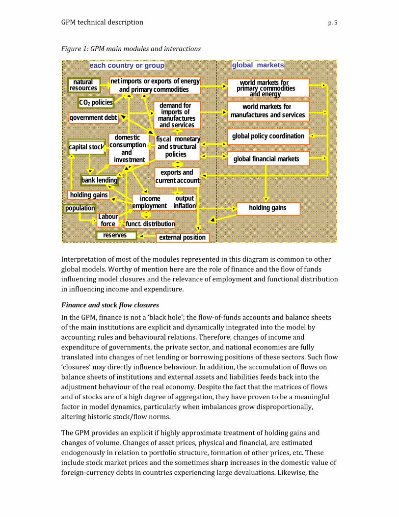
The GPM represents relationships between GDP, domestic demand, trade of various types of commodities and services and the balance of payments as feedbacks between flows of expenditure and income, mediated by policies and the financial conditions of main institutional sectors. These relationships are in turn affected endogenously by employment and distributional conditions. Meanwhile, global conditions in financial markets, as well as price formation in international markets tend to play a somewhat more independent role, wherein the influence of the specific country is more limited (see Figure 1).
GPM technical description p. 5
Figure 1: GPM main modules and interactions
Interpretation of most of the modules represented in this diagram is common to other global models. Worthy of mention here are the role of finance and the flow of funds influencing model closures and the relevance of employment and functional distribution in influencing income and expenditure.
Finance and stock flow closures
In the GPM, finance is not a ‘black hole’; the flow‐of‐funds accounts and balance sheets of the main institutions are explicit and dynamically integrated into the model by accounting rules and behavioural relations. Therefore, changes of income and expenditure of governments, the private sector, and national economies are fully translated into changes of net lending or borrowing positions of these sectors. Such flow ‘closures’ may directly influence behaviour. In addition, the accumulation of flows on balance sheets of institutions and external assets and liabilities feeds back into the adjustment behaviour of the real economy. Despite the fact that the matrices of flows and of stocks are of a high degree of aggregation, they have proven to be a meaningful factor in model dynamics, particularly when imbalances grow disproportionally, altering historic stock/flow norms.
The GPM provides an explicit if highly approximate treatment of holding gains and changes of volume. Changes of asset prices, physical and financial, are estimated endogenously in relation to portfolio structure, formation of other prices, etc. These include stock market prices and the sometimes sharp increases in the domestic value of foreign‐currency debts in countries experiencing large devaluations. Likewise, the
each country or group
exports andcurrent account
world markets for primary commodities
and energy
net imports or exports of energy and primary commodities
domestic consumption
andinvestment
income output,
employment inflation
global financial markets
fiscal, monetaryand structural
policies
global policy coordination
world markets for manufactures and services
demand forimports of
manufacturesand services
capital stock
bank lending
government debt
holding gains
holding gains
natural resources
population Labour force reserves
funct. distribution
CO2 policies
global markets
external position

GPM technical description p. 6
appreciation in value of external assets relative to liabilities of the USA, reflecting the declining international value of the dollar, are also considered. Other examples of such changes at balance sheet level include the impact of so‐called ‘inflation tax’ on the value of outstanding government debt, the effects of privatisations and bail‐outs, as well as haircuts that affect the growth of domestic and external debt
The relationship between the real economy (trade, production, income, spending etc.) and the financial system (deposits, debt, stocks and other types of financial asset and liability) in the GPM may be summarised as follows:
(i) real flows are necessarily matched by opposite financial flows and therefore in the short run may be said to constrain the latter on a net basis (so‐called financial balances)
(ii) gross flows of financial assets are largely determined by what may be described as 'financial' behaviour, subject to the constraints implied by (i) and recognizing that much financial behaviour has its roots in real economy opportunities and requirements
(iii) gross financial positions (accumulating flows and revaluations) feed back into real behaviour.3
The typical strength and speed of the various feed‐backs is largely an empirical matter requiring examination of the design and estimation of individual behavioural equations and checks on the realism of implied dynamics of the model at country level and for the world as a whole.
Although the logical structure of real and financial stocks, flows and holding gains is clear, behavioural feedbacks within the financial system and between the real economy and the financial system require ongoing research. The most critical aspect for international policy is the behaviour of external capital flows and their impacts on international positions and domestic financial markets that too often prejudice policies for the real economy.
Demographics, labour and income distribution
The GPM structure incorporates changing demographics, urbanisation and international migration, patterns of employment and GDP by broad sector and primary income distribution (the division of GDP between profits, mixed income and compensation of employees, and indirect taxation). These variables feed back into overall model dynamics and are important for policy evaluation.
Historical data demonstrate that increased urbanisation and a falling share of employment in agriculture in employment are universal trends that have reached very different stages in each part of the world but continue in all countries, the only
3 GPM equations for savings, investment, government revenue and spending and exchanges rates include balance‐sheet feedbacks but estimated coefficients are often too weak to exert any rapid effect and prevent accumulation of increasingly unbalanced positions.
GPM technical description p. 7
exceptions being short‐term reversals with returns to the countryside in times of extreme crisis.
The review of employment data also shows clear trends. Employment in services tends to increase as employment in agriculture falls and as the industrial labour force declines in countries where a large proportion of the labour force was formerly employed in manufacturing industries. Employment rates vary, depending on the level of participation of women and elderly people. Trend adult unemployment rates have remained below 10% in nearly all countries, with short‐term unemployment being more sensitive to the macro‐economic cycle in high income countries, particularly after the global financial crisis and ensuing deflationary policies. Youth unemployment has been high, rising recently in many countries despite widespread reductions in the number of young people coming into the labour force. Participation of young people in the labour force has fallen in most countries due to extension of secondary and tertiary education and training, facilitated by falling birth rates and reduced numbers of children as a percentage of population.
Differences and trends in primary income distribution in countries at different levels of development are less systematic, with particularly large gaps and some uncertainties about the interpretation of available data. The main generalisation that can be made is that the share of profits and mixed incomes in GDP is typically lower in developed countries and higher in developing countries where wages and salaries take a minor share. Long‐term declines in labour income shares (wages plus mixed incomes as proportion of GDP) can be observed over the last 20 to 30 years in many countries although the speed of the decline has somehow slowed‐down in recent years. It seems likely that higher monopoly power of corporate business, often linked to state de‐regulation, is an important factor for such a historic compression of labour income shares.
The inclusion of employment and primary income distribution makes it possible to model domestic inflation explicitly as an interaction between growth of earnings, aggregate productivity and profit mark‐ups and to trace the impact of changes in the share of profits on savings, portfolio and real expenditure. Employment levels, as well as changes in the distribution between profits and labour income may have significant impact on patterns of household consumption and investment spending. Increases in employment levels and economic activity, both in the short and long run, are stimulated by sustained growth of aggregate demand, which is the main trigger of productivity growth (à la Kaldor‐Verdoorn).
Patterns of functional income distribution have a strong path‐dependency but can adjust in response to various factors including fluctuations in activity and the terms of trade, public policy and incentives and longer‐run institutional changes. Changes in functional income distribution have a double effect. Higher profit mark‐ups tend to have a positive, albeit moderate and short‐term impact on investment. But such shifts also impact labour income, having a negative impact on consumer spending. The net impacts

GPM technical description p. 8
of increases in the mark‐up on growth of final demand and GDP are negative, with different degrees according to the context. Finally, the aggregation of these influences in a global model reveals large cross‐border spillovers and synchronised 'confidence' effects, which makes the call for global coordination of demand management particularly relevant.
BEHAVIOURAL EQUATIONS
Domestic macroeconomic and financial variables in equations discussed below are measured in real terms using a deflator for each country that compensates for inflation of the price of total domestic expenditure and for cross‐country differences in purchasing power. Meanwhile, international transactions and assets are measured in world‐average purchasing power. Volumes of GDP and traded goods and services are measured at constant prices while physical energy series (which can be solid, liquid, gas, electricity and other sources) are expressed in oil‐equivalent units. The GPM also models inflation of costs and final prices, nominal interest rates and exchange rate movements. Current dollar values of GDP, domestic income and expenditure, trade and the balance of payments and financial assets and liabilities are derived by multiplying real values by the appropriate deflator.
The GPM ensures global consistency of all external transactions, values of external assets and liabilities and real and nominal exchange rates. This is achieved by dynamic iteration of scaling adjustments on unadjusted values.4
Unless otherwise specified, variables in equations discussed below are specific of the country or group of countries, and measured by annual time series. World variables are denominated with the suffix W. Lagged variables are represented by subscripts ‐1, ‐2 etc.
Income and expenditure
Gross national income Y is distributed and spent by government on the one hand and the private sector (including households, corporations and state enterprises) on the other. The sources of gross national income are output (GDP), net receipts of external factor income and transfer payments and terms of trade effects.5
The private sector
Private disposable income is defined as national income not absorbed by the government (Yp = Y – Yg). Three main relations define private spending behaviour. Consumption (C = Yp – Sp) is determined by the savings function
4 Exceptionally physical energy is balanced for the world as a whole by the endogenous adjustment of the world price of oil. Other scaling adjustments are documented in the addendum, which provides definitions of unadjusted and adjusted versions of each variable. 5 Additions to or subtractions from the purchasing power of income generated by domestic output arising from changes in import and export prices
GPM technical description p. 9
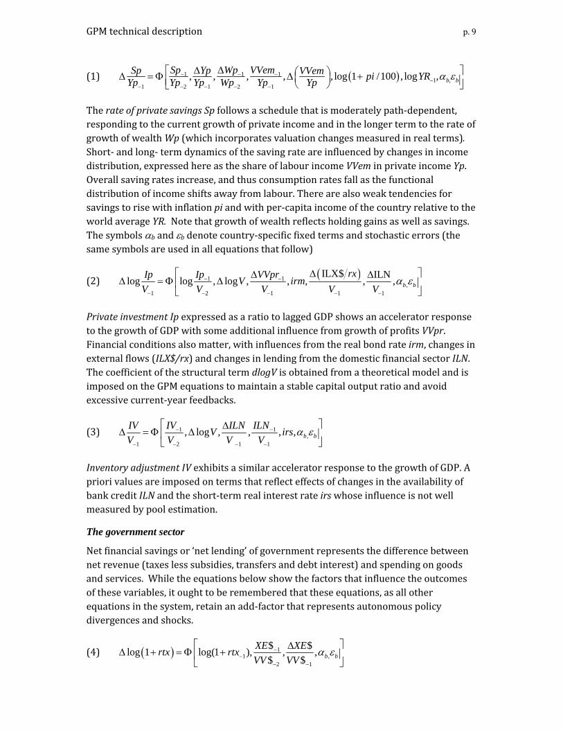
(1) ( )1 1 11 ,
1 2 1 2 1, , , , , log 1 /100 , log , b b
Sp Wp VVemSp Yp VVem pi YRYp Yp Yp Wp Yp Yp α ε− − −−
− − − − −
ΔΔ⎡ ⎤⎛ ⎞Δ = Φ Δ +⎜ ⎟⎢ ⎥⎝ ⎠⎣ ⎦
The rate of private savings Sp follows a schedule that is moderately path‐dependent, responding to the current growth of private income and in the longer term to the rate of growth of wealth Wp (which incorporates valuation changes measured in real terms). Short‐ and long‐ term dynamics of the saving rate are influenced by changes in income distribution, expressed here as the share of labour income VVem in private income Yp. Overall saving rates increase, and thus consumption rates fall as the functional distribution of income shifts away from labour. There are also weak tendencies for savings to rise with inflation pi and with per‐capita income of the country relative to the world average YR. Note that growth of wealth reflects holding gains as well as savings. The symbols αb and εb denote country‐specific fixed terms and stochastic errors (the same symbols are used in all equations that follow)
(2) ( )1 1,
1 2 1 1 1
ILX$ ILNlog log , log , , , , , b b
rxIp VVprIp V irmV V V V V
α ε− −
− − − − −
Δ⎡ ⎤Δ ΔΔ = Φ Δ⎢ ⎥
⎣ ⎦
Private investment Ip expressed as a ratio to lagged GDP shows an accelerator response to the growth of GDP with some additional influence from growth of profits VVpr. Financial conditions also matter, with influences from the real bond rate irm, changes in external flows (ILX$/rx) and changes in lending from the domestic financial sector ILN. The coefficient of the structural term dlogV is obtained from a theoretical model and is imposed on the GPM equations to maintain a stable capital output ratio and avoid excessive current‐year feedbacks.
(3) 1 1,
1 2 1 1
, log , , , , b bIV ILNIV ILNV irs
V V V Vα ε− −
− − − −
⎡ ⎤ΔΔ = Φ Δ⎢ ⎥
⎣ ⎦
Inventory adjustment IV exhibits a similar accelerator response to the growth of GDP. A priori values are imposed on terms that reflect effects of changes in the availability of bank credit ILN and the short‐term real interest rate irs whose influence is not well measured by pool estimation.
The government sector
Net financial savings or ‘net lending’ of government represents the difference between net revenue (taxes less subsidies, transfers and debt interest) and spending on goods and services. While the equations below show the factors that influence the outcomes of these variables, it ought to be remembered that these equations, as all other equations in the system, retain an add‐factor that represents autonomous policy divergences and shocks.
(4) ( ) 11 ,
2 1
$ $log 1 log(1 ), , ,$ $ b b
XE XErtx rtxVV VV
α ε−−
− −
⎡ ⎤ΔΔ + = Φ +⎢ ⎥
⎣ ⎦

GPM technical description p. 10
The share of indirect taxes less subsidies in GDP, rtx, is strongly path dependent and is significantly influenced by the level and increase in the value of energy exports.
(5) 1 1 11 ,
1 1 2 1
log log , log , log , log , log , b bYgd Lg VVtxYgd Y Y NUL
Y Y Y Yα ε− − −
−− − − −
⎡ ⎤Δ = Φ Δ Δ Δ Δ⎢ ⎥
⎣ ⎦
Direct revenue net of transfers and interest payments Ygd rises or falls with gross national income Y with a lag. A high public debt ratio Lg/Y usually calls for long‐term increases in direct tax collection, while increases in proceeds of indirect taxation VVtx reduce the pressure to make savings on transfers or increase direct tax rates. An opposite effect is caused by fluctuations in the unemployment rate NUL.
(6) 1 1 1 11 1 1 ,
2 1 1 1
$log log , , log , log , log , log , ,$ b b
Yg Lg AGF CAG G N YRY Y Y Y
α ε− − − −− − −
− − − −
⎡ ⎤Δ = Φ Δ Δ⎢ ⎥
⎣ ⎦
Government spending on goods and services G shows a strong path‐dependency and is further influenced by financial conditions as well as external sustainability. It mostly responds to the performance of government income Yg and the composition of the balance sheet (Lg, government debt, and AGF, government financial assets). State variables like population, N, and the degree of development captured by relative income per capita YR, also have some influence. Finally, government spending on goods and services tends to respond to external performance, measured by the current account CA$.
Trade and the external current account The GPM models the current account in some detail, distinguishing the value and volume of exports and imports in four categories of trade ‐food and raw materials, energy, manufactures and services‐, as well as receipts and payments of income and transfers. Trade in manufactures is the clearest short‐run driver, responding to prices, exchange rates, growth and fluctuations in expenditure in all countries.
Trade in manufactured goods
Markets for manufactures are modelled on a bilateral basis that reflect the evolving pattern of linkages and network production systems between countries. Imports respond to activity, prices, the real exchange rate, etc, with the price being calculated as a weighted average of export prices of suppliers. Exports are determined by market shares (i.e. shares of each supplier in imports of each importing country). Market shares and export prices respond to relative unit costs, calculated as a weighted average of domestic costs and costs of imports of primary commodities, energy and services as well as manufactures).
(7) 11 1 0 ,log $ log $ , log $, log $ , log , log , b bMM MM MH MH pmm rx α ε−− −⎡ ⎤Δ = Φ Δ Δ⎣ ⎦

GPM technical description p. 11
The value of imports of manufactures MM$ responds to a weighted sum of expenditures MH$ that attributes relatively high import intensity to investment IP, IV and exports X$, and relatively low import intensity to government spending on goods and services G:
( )( )$ $ $0.4 2 2MH rx C G IP IV X XM= ⋅ + ⋅ + ⋅ + + + ⋅
Finally, the value of manufacturing imports is affected by changes in the real exchange rate rx and supplier prices pmm0. This equation also includes a long‐run trend, representing the momentum of globalisation.
(8) ( ) ( )1
1 10 00 00log log
$ $, log , log , ,b b
pmm MMpmm MM pmm rxMM MM
α ε−
− −Δ Δ Δ
⎧ ⎫⋅⋅ ⎪ ⎪= Φ⎨ ⎬⎪ ⎪⎩ ⎭
Given the value of imports measured in world purchasing power terms, movement of the volume of imports of manufactures MM0 is a question of changes in price. The model assumes a unit long‐run elasticity with respect to the weighted‐average supplier price, pmm0, and estimates short‐run coefficients to capture delays in passing through changes in supplier prices and the real exchange rate rx.
Global consistency is enforced by scaling import volumes to match export volumes in the world as a whole.
(9) ( ) ( ) ( ) ( )1 1 1$ $log log , log , log , ,b bsxm sxm ucx ucx α ε− − −ΔΔ⎧ ⎫= Φ⎨ ⎬⎩ ⎭
The value of exports XM$ of each country is determined by summing the product of imports by value in each importing market and the country’s market share as a supplier. Market shares sxm exhibit slow adjustment to unit costs ucx. The estimated long‐run elasticity of market share by value with respect to relative unit costs is around 3.6 Fixed effects are in this instance bilateral and differ substantially depending on the size and proximity of suppliers and import markets. Estimates generated by the equation above are scaled to sum to unity in each market.7
(10) 1001 1 ,
1
log log , log , log ,$ $ b b
XMXM ucx YRXM XM
α ε−− −
−
⎡ ⎤Δ = Φ ⎢ ⎥
⎣ ⎦
Given the value of exports of manufactures the volume of exports XM0 is again determined by price movements. In the long run aggregate manufacturing export prices
6 Coefficients are estimated using a panel that excludes supplier‐importer pairs with very low levels of trade for which market shares may exhibit erratic year‐on‐year proportionate changes.
7 This adjustment transforms the country‐level equations into an Armington‐style system in which market shares depend on trade‐weighted relative unit costs of the different suppliers.

GPM technical description p. 12
rise with unit costs of exports ucx$, while such effects are relatively weaker in more advanced countries (hence the introduction of the variable YR, relative income per capita), presumably reflecting their established presence in world markets through production networks and institutional ties.
Trade in services
The international market for services trade is set up as pool. Net exports of each country measured in international purchasing power depends on the real exchange rate and service requirements of different branches of merchandise trade. Imports are determined as a function of net exports and the same variables, leaving exports (gross) to be calculated as the balancing item. Global service trade is balanced by scaling exports to ensure that the world total is equal to world imports. Export and import volumes at base year dollar prices depend on values and on changes in the real exchange rate.
(11) ( )1 1 1 1
$ $ $$ log , , , , ,b bBS BA BE BMrxV V V V
α ε− − − −
Δ Δ Δ ΔΔ⎧ ⎫⎪ ⎪= Φ⎨ ⎬⎪ ⎪⎩ ⎭
(12) ( ) { }( )
1 1 1 1 1
min $$ $ $ $0,log , , , , , ,b b
BSMS MA XE MMrxV V V V V
α ε+
− − − − −
ΔΔ Δ Δ ΔΔ
⎧ ⎫⎪ ⎪= Φ⎨ ⎬⎪ ⎪⎩ ⎭
(13) 1001 ,
1
log log , log , log ,$ $ b b
MSMS rx YRMS MS
α ε−−
−
⎡ ⎤Δ = Φ Δ⎢ ⎥
⎣ ⎦
(14) 1001 ,
1
log log , log , log ,$ $ b b
XSXS rx YRXS XS
α ε−−
−
⎡ ⎤Δ = Φ Δ⎢ ⎥
⎣ ⎦
Trade in primary commodities
World markets for primary commodities are modelled as a pool system with price and quantity adjustments. A country‐level equation determines the balance of net exports or imports as an implicit function of domestic supply and demand. Imports of each country are then scaled to match total world exports. The world price index for primary commodities responds to the rate of growth of world imports.
(15) ⎥⎥⎦
⎤
⎢⎢⎣
⎡Δ
ΔΦ=
Δ
−−
bblpaV
VVBA
εα ,0
0
0
0 ,log,11
Net exports of primary commodities at base year prices BA0 expressed as a ratio to GDP fluctuate with the changes in GDP and tend to increase with a rise in lagged world prices lpa converted into domestic purchasing power terms.

GPM technical description p. 13
(16) { }( )00
1 1
max ,0, ,b b
BAXAV V
α ε− −
ΔΔ⎧ ⎫⎪ ⎪= Φ⎨ ⎬⎪ ⎪⎩ ⎭
The volume of exports of primary commodities at base year prices XA0 depends primarily on the availability of a net export surplus. The volume of imports MA0 is initially derived as a balancing item for each country but is then scaled to balance total imports and exports in the world as a whole. Finally the volume of net exports is adjusted to reflect the adjustment of import volume.
(17) ⎥⎦
⎤⎢⎣
⎡ΔΔΦ=Δ bbpp
rxwpaMAMA εα ,
00
,log,_log$log
Given the volume of imports, the value of imports of primary commodities MA$ is once again a function of price changes. Import prices responds positively to world prices pa_w and the real exchange rate rx. The latter is scaled to have a larger impact in countries with lower base‐year parities.
(18) 1 ,0 0
$log log _ , log , log , b bXA rxpa w YRXA pp
α ε−
⎡ ⎤Δ = Φ Δ Δ⎢ ⎥
⎣ ⎦
The value of exports of primary commodities XA$ responds similarly with an additional term implying slightly lower export prices in high income countries. Finally the value of exports is scaled to match the value of imports for the world as a whole.
Energy trade and environmental considerations
Energy production, demand and trade flows are determined in physical terms with supply and demand cleared by movements of the world price of oil. A distinction is made between carbon sources of supply (oil, gas and coal) and non‐carbon sources (mainly hydro and nuclear electricity) which have radically different implications for global emissions.
(19) 1
1 10 1log log log log ,log log , log , , , , , , b b
ED V IVN N V
ED lped tt X YrN
α ε−
− −
−Δ Δ Δ Δ Δ⎧ ⎫⎪ ⎪= Φ⎨ ⎬⎪ ⎪⎩ ⎭
Primary energy demand ED relative to population N fluctuates in the short run in response to changes in GDP per capita V/N, the terms of trade tt, export volume X0 and inventory adjustment IV. In the longer term it responds to the level of per capita income
GPM technical description p. 14
relative to the world average Yr and lagged changes in the world oil price converted to domestic purchasing power terms lped.8
(20) ⎥⎦
⎤⎢⎣
⎡Δ⎟⎟
⎠
⎞⎜⎜⎝
⎛ΔΦ=Δ
−
−bblpep
EPED
EDEPc εα ,1
1 ,log,1,minloglog
Annual changes in production of carbon energy EPc are largely driven by growth of domestic demand ED9 and are influenced by another lagged oil price indicator lpep.10 Differences in resources and market access are reflected in country‐specific intercepts.
(21) ⎥⎦
⎤⎢⎣
⎡ΔΦ=Δ
−−
−
bbn lpepcED
EDmavEP
EDmavEPn εα ,
21
,,log,)(
log)(
log 1
Production of noncarbon energy EPn is assumed to adjust to the lagged moving‐average level of domestic energy demand as well as short‐term fluctuations and a modified lagged oil price indicator that can take account of ‘carbon‐taxes’ when applicable lpepc.11
(22)
( )( ) ( )( )[ ]bbwEPEPEDEMEPEDEM εα ,111 ,_log,0,maxlog0,maxlog Δ−−Φ=−−Δ −−−
Energy imports EM in excess of the amount required to fill the gap between domestic demand and supply are assumed to increase with growth of global supply EP_w. Exports are derived as the balancing item in energy supply and demand for each country.
(23) 12,
1 1
2log log , log , log 2, b b
COCO Yn lttcoED EPn ED EPn
α ε−
− −
⎡ ⎤Δ = Φ ⎢ ⎥− −⎣ ⎦
Carbon emissions CO2 are modelled as a function of carbon energy use (EDEPn) and imputed carbon taxes (tttco2), with trends also influenced by the level of income per‐capita Yn.
The world oil price pe_w is solved endogenously to find the value that equalizes total world supply and demand for energy expressed in tons of oil equivalent. Auxiliary
8 This term is a moving average of prior‐year values and incorporates a transform to introduce the notion of a real oil price ceiling with energy demand and supply becoming increasingly price‐elastic as the ceiling is approached. 9 In case of a country with very large non‐carbon sources, this equation is modified to suppress the linkage between carbon energy supply and domestic energy demand. 10 See the footnote for energy demand. 11 In simulations this variable may be loaded with a carbon tax to simulate penalties on use of fuels that generate high CO2 emissions.

GPM technical description p. 15
equations convert physical imports and exports into imports and exports measured at base‐year dollar prices ME0 and XE0 and the world oil price is used to estimate values of imports and exports ME$ and XE$ in international purchasing power terms.
External income and transfers
(24) 1 1
1 1 1 1
$ $$ $
$ $ $ $, , , ,US b bim
BIT NXBIT NXY Y Y Y
α ε− −
− − − −
Δ Δ⎧ ⎫⎪ ⎪= Φ ⋅⎨ ⎬⎪ ⎪⎩ ⎭
Net income and transfers, BIT$, is estimated as a balance to improve stability responding to the inherited net external position NX$ which when multiplied by the interest rate of US Treasuries, imUS, serves as a proxy for flows of factor revenue.
Movements of receipts XIT$ and payments MIT$ on the external income and transfers account, are estimated by generating a proxy NIT$, termed “covered” income and transfers, that represents the minimum of the two:
$ $ $$
$ $ $
XIT if XIT MITNIT
MIT if XIT MIT≤⎧
= ⎨ >⎩
The model can then impute receipts and payments separately using the figure for net income and transfers from the equation above. 12
(25) 1 1, 1 ,log $ log $ , log $ log $ _ , log , b bNIT NIT NXN X w YR α ε− − −⎡ ⎤Δ = Φ Δ⎣ ⎦
The “covered” flow so defined is moderately path‐dependent and is correlated with the level of net external assets and liabilities NXN$ (defined as a “covered” position in similar fashion) and global trade, X$_w. These relations depend on the degree of development, again captured by relative income per capita YR.
Specification of exports and imports in value and volume terms and flows of external income and transfers completes modelling of the trade balance and current account. Together with the modules covering government and non‐government income and expenditure and standard national accounting identities, these equations are sufficient to determine GDP (output), the terms of trade and gross national income.
The financial sector: flow of funds, holding gains and balances
Modelling of assets and liabilities, even if at very high degree of aggregation, provides a method for monitoring the plausibility of ongoing financial imbalances (flows) that may or may not result in acceptable accumulation of assets and liabilities (stocks) as time goes by. Also, it adds an anchor to the adjustments in the real economy by allowing balances of institutions to feed back into spending behaviour and policy reactions. The main difficulty, apart from paucity and unreliability of data, is that stocks may also be 12 XIT$ = NIT$ + max(BIT$,0) MIT$ = NIT$ + max(BIT$,0)

GPM technical description p. 16
strongly influenced by holding gains and losses. The GPM does not attempt a detailed asset pricing model or sophisticated analysis of portfolio behaviour of households, corporations, financial institutions etc. but the simplified price functions and balance sheet closures represented in the model serve to trace movements of the main financial variables on annual basis. Non‐government sectors including state enterprises are aggregated into a single group, the private sector, which excludes the domestic banking sector for which separate data are available for virtually all countries. External assets and liabilities are modelled on a gross basis. Together with government balances these balance sheets provide a consistent breakdown of national wealth for each country or country group.
The matrix below shows assets and liabilities considered from the perspective of a single country. The matrix format makes it evident that every asset has an issuer for which it is a liability as well as a holder. For consistency the model ensures that total external assets and liabilities shown in the row for the rest of the world, measured in international purchasing power, are equal when summed over all countries. Net worth of the banking system is assumed to be zero (capital of banks is included in assets held by government, AGF, and other sectors, DP).
Matrix of assets and liabilities
Assets (held by) Banks Government Non-government Rest of world
Net worth
Capital stock KP Liabilities of Banks Agf DP 0 Government Lgf Lgo (1) Non-government LN Lx$/rx WP Rest of world R$/rx Axo$/rx (1) -Nx$/rx
(1) A portion of Lgo and Lx$/rx represents government debt held by non‐residents and a portion of Axo$ represents external assets held by government. This does not invalidate the wealth identities (Nx$ = Lx$ R$ Axo$ and WP = DP + Lgo + Axo$/rx LN Lx$/rx).
For each asset identified in the matrix, the GPM tracks cash flows and holding gains or losses. The flow of funds matrix in the next table below shows the cash flows and savings by which they are financed. 13 Again, every asset transaction has a buyer and seller so that all cash is accounted for, at least on a net basis.
13 The table includes one cash flow, IAgo, for which there is no corresponding asset in the matrix above due to lack of data on the value of government‐owned equity and lending to state enterprises and the private sector. By necessity these items that represent liabilities of the non‐government sector are omitted from the calculation of private wealth, WP.

GPM technical description p. 17
Summary flowoffunds matrix
Uses of funds / net acquisition of assets Sources of funds
Banks Government Non-government Rest of world Net lending
Capital stock Ip + IV Issuers Banks IAgf IDP 0 Government ILgf ILgo (1) Yg - G Non-government ILN IAgo ILx$/rx Sp-Ip-IV Rest of world IR$/rx IAxo$/rx (1) -CA$/rx
(1) See the note to the preceding table.
The following sub‐sections show how the GPM models asset holdings, gains and losses and cash flows for each sector identified in these tables.
Government debt and asset transactions
The determination of changes in outstanding government debt Lg starts with net lending NLg which represents the difference between government income Yg and spending G discussed above.
The accumulation of government debt is affected by asset transactions, debt write‐offs and, in the case of foreign currency debt, exchange rate movements.14 Historical data often show large discrepancies between government net lending and changes in outstanding debt that cannot readily be explained by revaluation effects. The discrepancy is usually the result of asset transactions such as lending and capital transfers to state enterprises, the private sector and foreign governments and proceeds of privatisation. To track the accumulation of government debt it is necessary to model the aggregate of these transactions as well as any debt forgiveness or write‐offs.
The GPM divides government asset transactions between deposits and investment in the banking sector and transactions with the rest of the economy. Injections or accumulation of deposits with the banking sector IAgf are treated as consequence of balance sheet requirements of government and banks, discussed further below. Net asset transactions with the rest of the economy IAgo are modelled directly as a cash flow since data on corresponding assets are not available. Historical estimates of the cash flow are derived as a residual of government accounts after an approximate estimation of holding gains15 and the net figure is treated as a contribution to changes in private wealth Wp but not income.
14 Measured in real terms outstanding debt is also affected by inflation which reduces its value or deflation (a falling price level) which increases its value. 15 Since historical series on debt write‐offs are not available, write‐offs are implicitly included with asset transactions.
GPM technical description p. 18
(26) ( ) ( )
1
1 1 1
, , ,b bLgIAgo NLg
Y Y Yα ε
− +
−
− − −
⎧ ⎫⎪ ⎪= Φ⎨ ⎬⎪ ⎪⎩ ⎭
Government asset transactions with the rest of the economy IAgo are negatively correlated with outstanding debt Lg and positively correlated with government net lending NLg.
Given net lending, holding gains16 and asset transactions with the rest of the economy, there is an implied change in the government’s financial position Ngf defined as the value of deposits and investments in the domestic banking system less outstanding debt. This may be positive or negative depending on whether the government is a net creditor or debtor and the net figure is not sufficient by itself to determine each side of the balance sheet. Therefore the GPM sets a floor using a proxy variable termed covered government debt Ngi defined as the minimum of assets Agf and debt liabilities Lg. If sustained cash surpluses reduce outstanding debt to the minimum level further net cash receipts accumulate as deposits in the banking system. If on the other hand government is short of cash and deposits with the banking system are at a minimum level, further cash outlays must be financed by increases in outstanding debt.
(27) 11 1 ,
1
$log log , log , log , log , b bRNgi Ngi Y YRrx
α ε−− −
−
⎡ ⎤Δ = Φ Δ⎢ ⎥
⎣ ⎦
Covered government debt, so defined, is positively correlated with national income Y, the accumulated stock of foreign exchange reserves measured in domestic purchasing power R$/rx and the degree of development represented by the YR variable
Given the level of covered debt and the government's net financial position, the derivation of assets Agf and liabilities Lg follows. Calculation of the net cash flow IAgf required to maintain government’s investment and deposits with the banking system Agf requires estimation of capital gains or losses. The GPM makes the somewhat heroic assumption that government ultimately absorbs 70% of losses arising from abnormal debt write‐offs by banks as well as gains or losses on exchange reserves held by the central bank which from an accounting perspective is part of the domestic banking system.
The remaining task to complete the government’s balance sheet is estimation of the split between government debt held by the domestic banking system and other holders.
(28) 11
1
log log , log , , bDPLgo YR
Lg Yα ε−
−−
⎡ ⎤Δ = Φ Δ⎢ ⎥
⎣ ⎦
16 Holding gains or losses in government accounts depend on changes in the real value of deposits and investments in the banking system as well as changes in the real value of outstanding debt.
GPM technical description p. 19
Nonbank holdings of government debt Lg0 as a share of total debt outstanding Lg 17 respond weakly to prior‐year growth of bank deposits DP and are also influenced by the degree of development again represented by relative income per capita YR.
Cash flows ILgo and ILgf follow from changes in values of outstanding debt after allowing for holding gains or losses.18
The external position and exchange rates
The external position may be understood as representing the accumulation of current account surpluses and deficits and holding gains or losses on external assets and liabilities. Changes in market positions are also influenced by acquisition or sale of exchange reserves by the monetary authority.
(29) ( ) 1
1 1 1
$$ $$
$ $log log , , , ,b b
CAR CArprrx Y Y Y
α ε−
− − −
Δ⎧ ⎫⎪ ⎪= Φ⎨ ⎬⋅ ⎪ ⎪⎩ ⎭
Exchange reserves, denominated in domestic purchasing power dollars, R$/rx , are modelled as a ratio to national income. 19 The reserve ratio responds to valuation changes rpr$ and is positively correlated with the current account outturn CA$. The equation has large residuals reflecting changes in central bank policy.
Given the movement of exchange reserves, changes in the net market position Nxf$ are fully determined by the balance on current account, together with holding gains and losses. The covered market position Nxi$ defined as the minimum of non‐reserve assets and liabilities, is modelled as follows.
(30) [ ]bYRYrxYNxi εα ,,log,$log,loglog 111
1−−−
−
ΔΔΦ=Δ
The covered position which may also be viewed as an indicator of 'openness' of the external capital account has historically increased in an uneven and highly path‐dependent manner. Countries with major global financial centres such as the US and the UK have far higher levels of external assets and liabilities relative to the size of their domestic economies than others and countries with managed exchange regimes may have very low levels of recorded non‐reserve assets. Beyond these country‐specific factors the covered position typically responds to the level and growth of national income Y and reserves R$. Together with the net market position Nxf representing the
17 A slightly more complex transform is used in the model to keep the share below unity. 18 When historical time series are lacking or incomplete, the GPM assumes that government debt denominated in foreign currency diminishes with a rising level of per capita GDP. Erosion of the value of domestic currency debt is determined by domestic price inflation. 19 Once again the model uses a slightly more complex function to impose a ceiling on exchange reserves relative to annual income.

GPM technical description p. 20
accumulation of current account and reserve transactions and revaluations, the degree of openness determines total external assets Axo$ and liabilities Lx$.
Exchange rates
The real exchange rate represents the combined effect of changes in domestic and external price levels and changes in nominal exchange rates. The real exchange rate that results is critical for the determination of relative prices of domestic and external goods and services and unit costs in each country relative to competitors. Since participants in exchange markets can be assumed to be well aware of the need for nominal exchange rate movements to compensate for differences in inflation, the GPM models the real exchange rate directly, leaving nominal exchange rate movements to be inferred as the consequence of changes in the real exchange rate and differential rates of inflation.
(31) ( ) 21 1
5
log log , log 1 , log _ , log , log , , bVrx rx rxna ph w YR
Vα ε− −
−
⎡ ⎤Δ = Φ Δ + Δ Δ⎢ ⎥
⎣ ⎦
The real exchange rx rises in the long run with sustained GDP growth and increases in relative income per capita YR. In the short run it fluctuates in response to nominal exchange rate changes rxna and changes in global inflation ph_w. Inevitably there are significant fixed effects and large residuals reflecting differences in financial systems and exchange regimes as well as changing market expectations about future economic growth and trade prospects of individual countries. 20
Revaluation of external assets and liabilities
(32) ( ) [ ]bbwphrpr εα ,,_log$1log ΔΦ=+
(33) [ ]1log $ log _ , log , ,b brpaxo ph w YR α ε−= Φ Δ
(34) [ ]bbpkpwphrplx εα ,,log,_log$log ΔΔΦ=
The real value of external assets in international purchasing power (reserves rpr$, other assets rpaxo$ and liabilities rplx$) is eroded by world inflation Δlog(ph_w). Liabilities appreciate with a rise in the real price of capital assets pkp in each country while gains in the real value of other assets tends to be lower in countries with higher relative income YR.
Real values in domestic terms are further affected by movements in the real exchange rate giving rise to additional holding gains or losses in the balance sheets of domestic residents.
20 Exchange rates whether nominal or real have one less degree of freedom than the number of countries since they represent relative rather than absolute prices. The GPM determines the real exchange rate for each country independently in the first instance and makes a scaling correction for all countries to maintain consistency for the world as a whole.
GPM technical description p. 21
An important issue for open economies with large financial sectors is the movement of asset prices relative to liabilities which may, as in the case of the USA when the dollar experiences a significant depreciation, generating net holding gains as foreign‐currency assets appreciate relative to dollar liabilities on a scale sufficient to compensate substantial current account deficits. By implication other countries experience holding losses as their dollar assets depreciate relative to non‐dollar liabilities. These effects which make the relationship between international positions and current accounts highly uncertain in the longer run are another subject of continuing research.
The domestic banking system
The final component of domestic balance sheets is assets and liabilities of the banking system. Exchange reserves R$/rx, government investment in banks Agf and liabilities to banks Lgf have already been discussed. The remaining components of the balance sheet of the domestic banking system are domestic lending LN and, as a balancing item, other liabilities DP including capital and net external liabilities as well as domestic deposits. The two items LN and DP are again modelled by considering the net position, Nff, which may in principal be positive or negative, and the covered position, Nfi, formally defined as the minimum of lending to the private sector LN and liabilities DP. In practice Nfi nearly always represents lending as the banking system's net position with the private sector Nff is positive and deposits are the larger of the two. In periods of credit expansion loans and deposits rise together, represented by increasing Nfi .
The net position of the domestic banking system with the private sector Nff is given by the three factors mentioned earlier ‐ reserves R, government assets Agf and government debt held by banks Lgf.
Expansion or contraction of the covered position Nfi representing lending to the private sector is modelled as follows:
(35)
( )
1 1 11
1 1 1 1 1 1 1
$$$
log log , log , log , , , , , , ,b bNff Nff LgfNfi Nfi LN
Nfi R NxiNfi WLNAY YY Y Y Y
α ε−
− − −−
− − − − − − −
Δ ΔΔ Δ
⎧ ⎫⎪ ⎪+
= Φ⎨ ⎬⎪ ⎪⎩ ⎭
Thus, the ratio of covered bank lending to income Nfi/Y(1)21 responds positively to income Y, excess deposits Nff, liquidity in the form of government debt LGF, and the size of the external position R$ + Nxi$. Past debt write‐offs WLNA are included as an
21 This ratio is written in a form that imposes a ceiling equal to 2.5 times annual income.

GPM technical description p. 22
exogenous variable whose value can be specified in scenarios to simulate the impact of a financial crisis.22
The net position and covered lending determine loans LN and liabilities DP. Cash flows are again derived by subtracting estimated holding gains from balance sheet changes. 23
Capital stock and private wealth
Financial components of private wealth have now been fully accounted for. It remains to consider the value of the capital stock which includes land, produced capital goods and IPR. Like many other macro‐models the GPM calculates the stock of produced capital goods KI by the perpetual inventory method, accumulating investment in capital goods and inventory, IP + IV, in each period and deducting an estimate for capital consumption.
(36) ( ) ( ) ( )1 1log log log log, , , ,b bpkpVpkp pkp
VTα ε− −Δ Δ
⎧ ⎫⎪ ⎪= Φ⎨ ⎬⎪ ⎪⎩ ⎭
The real price of capital pkp is modelled as a path‐dependent variable with momentum represented by the lagged dlog(pkp) term, responding to the level of capacity utilization V/VT. The value of the capital stock is then calculated as the product of the stock of produced capital goods KI and the real price of capital.
Private wealth Wp is defined as the sum of the real value of capital and net financial assets of the private sector. Changes in private wealth are identically equal to the sum of savings, net receipts from government asset transactions and holding gains and losses less capital consumption.
Interest rates24
The GPM models two interest rates for each country a short‐term ‘policy’ rate is and a longer‐term bond rate im.
22 In this case again the lack of historical time series means that modelling has to be based on a priori assumptions that cannot be tested systematically. 23 This time holding gains or losses exclude items such as gains on exchange reserves and 70% of losses on abnormal debt write‐offs that are absorbed by government.
24 A comment is necessary on the measurement procedure and significance of series for interest rates and inflation for countries that comprise countries using different currencies. The GPM measures nominal interest rates and inflation as weighted averages using ppp expenditure in each country as the weighting factor. This procedure has some drawbacks when very different rates of inflation are experienced in countries belonging to a group of countries in the GPM. These are familiar problems affecting regional currency agreements as well.

GPM technical description p. 23
(37) ( ) ( ) ( ) ( )( )
( ) ( ) ( )
1 1log log , log , log , log , ,b bVis is pi pi
VTα ε
+− + +
− −Δ Δ⎧ ⎫⎪ ⎪= Φ⎨ ⎬⎪ ⎪⎩ ⎭
Changes in the policy rate is25 follow a Taylor rule determined by domestic inflation pi and capacity utilization, V/VT.
(38) 11 1
1
log log , log , log , log , log , ,b bVVim is is pvi pviN
α ε−− −
−
⎡ ⎤= Φ Δ Δ⎢ ⎥
⎣ ⎦
The bond rate im responds to the level and rate of change of the policy rate is and cost inflation pvi with a tendency to be lower in countries with higher GDP per capita VV/N.
Inflation and employment
Price formation
Domestic cost inflation pvi is modelled as the outcome of increases in unit labour cost, determined by changes in average money earnings ei and output per person employed V/NE with a variable profit markup mu and a further markup for indirect taxes less subsidies rtx discussed in the section of government income and expenditure. Thus
( ) 1 1
1 1
/ 1 11 1/ 1 1
V NE mu rtxpvi eiV NE mu rtx− −
− −
⎡ ⎤+ ++ = + ⎢ ⎥+ +⎣ ⎦
(39) 1 1 1 1log log , log , log , log , log , ,b bVei ei pi rx YRNE
α ε− − − −⎡ ⎤Δ = Φ Δ⎢ ⎥⎣ ⎦
Average earnings per person employed ei26 respond to increases in output per person employed V/NE and, with some lag, to price inflation pi, with negative pressure exerted by a higher real exchange rate rx, influenced by the relative income per capita YR
(40)
( ) ( ) ( )11 1
$log 1 log 1 , log 1 , log , log , , log , , ,b bV LN G XEmu mu ei ttNE VV VV rxVV
α ε−− −
⎡ ⎤Δ + = Φ + + Δ Δ Δ Δ Δ⎢ ⎥
⎣ ⎦
The profit markup on average unit labour cost mu is strongly path dependent and in the short run responds to the interaction between forces driving wage costs, ei on the one hand and productivity growth V/NE, on the other. The mark‐up is also affected by credit
25 The GPM uses a modified transform that allows negative interest rates as these are sometimes found in estimated historical data. This problem should be eliminated by data improvements. 26 The model includes a constant that allows for reductions in average earnings per person in case of deflation or economic crisis.

GPM technical description p. 24
conditions LN/VV, government policies including social protection and government employment G/VV, movements of the terms of trade tt and energy exports XE$.
The distribution of GDP between labour income VVEM and profits VVPR27 is largely determined by the profit markup.
Domestic price inflation, pi, measured as annual changes in the domestic expenditure deflator, is the outcome of cost inflation and movements of the terms of trade and is derived by an identity which is a consequence of national accounting definitions. If the terms of trade move in a country’s favour, a greater proportion of domestic costs are passed through to exports and/or import prices fall to the benefit of the domestic market. However higher export prices do not by themselves reduce domestic inflation. Indeed an increase in export prices usually implies higher costs or profits of producers which may result in higher domestic prices. The terms of trade benefit to domestic price inflation only takes effect if and when import prices fall or rise less than export prices while domestic costs (including profit) fall or remain unchanged.
Employment
Employment is analyzed separately for male and female members of the labour force, distinguishing young persons aged 15‐24 and adults aged 25 and over. The starting point is participation in the labour force, generally represented as a percentage of the relevant population. Unemployment rates are modelled explicitly as functions of economic activity and employment is derived by identity as the number of persons in the labour force less those unemployed.
(41) [ ]1 1log log , , , , log , ,b bNLNga NLNga NONga NCNga NURN YR α ε− −Δ = Φ
Labour force participation for each gender “g” and age‐group “a” NLNga tends to reduce with urbanisation NURN but may increase slightly with GDP per capita. Adult participation defined relative to the entire population aged 25 or over falls with ageing NONga while participation of young persons is higher in countries with larger numbers of children NCNga. Adult male participation rates tend to be slightly higher, and adult female rates lower, in countries with higher income YR.
In the GPM panel labour force participation does not show a significant cyclical component. The clearest longer‐term trend is a reduction in participation of young persons as the number of children declines and secondary and tertiary education are extended.
27 In the GPM labour income includes the national accounting categories ‘compensation of employees’ and ‘mixed income’ and profits are represented by the ‘operating surplus’. Employment includes employees, self‐employed and family workers.

GPM technical description p. 25
(42)
1 1log log , log , log , log , log , , , ,b bIVwNULga NULga Nga V V IP NURNVw
β β β α ε− −⎡ ⎤Δ = Φ Δ Δ Δ Δ⎢ ⎥⎣ ⎦
The unemployment rate for each gender ‘g’ and age group ‘a’ NULga increases with faster growth of population Nga and fluctuates in response to growth of activity V and investment IP with a significant impact of the global cycle represented by world inventory changes IVw. Unemployment rates also tend to rise with urbanisation. The coefficient β multiplying activity and investment terms in the equation above represents a response that increases with the relative income level YR.
Aggregate employment NEga for each gender ‘g’ and age group ‘a’ is obtained by multiplying population by the participation rate and subtracting the number of unemployed. Total employment NE is the sum of employment for each gender and age group.
(43) ( )[ ]bbVVVVNURN εα ,,3//loglog 3−Φ=Δ
Urbanization NURN is a long‐term ongoing process that shows some response to GDP growth. 28
(44) 11
1 2
log 1 log 1 , , log , ,b bNIMNIM YR NE
NE NEα ε−
−− −
⎡ ⎤⎛ ⎞ ⎛ ⎞Δ + = Φ + Δ⎢ ⎥⎜ ⎟ ⎜ ⎟
⎝ ⎠ ⎝ ⎠⎣ ⎦
Growth of population of working age is affected by net migration NIM responding to the relative income level and growth of employment in the country. 29
The GPM includes a provisional analysis of employment by gender and broad sector with estimates of GDP by broad sector for comparison. Another preliminary development is a breakdown of total employment between employees and other categories of worker (self‐employed and family workers) with a matching breakdown of labour income between compensation of employees and mixed income.
SELECTED MULTIPLIER TABLES
Apart from econometric properties of the equations specified above, which are captured by the usual tests, an important quality of a complex model is its ability to generate plausible results when shocks to behavioural equations play out through the model as a whole. This is the essence of ‘multiplier analysis’, which highlights the model's ability to capture not only feedbacks internal to a particular economy but also those which result
28 The LHS is formulated to constrain the share of urban population to the range zero to 1. 29 The increase in population in each age group is exogenous (based on UN projections).
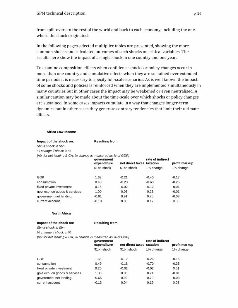
GPM technical description p. 26
from spill‐overs to the rest of the world and back to each economy, including the one where the shock originated.
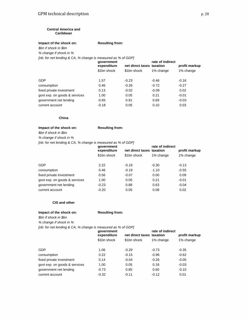
In the following pages selected multiplier tables are presented, showing the more common shocks and calculated outcomes of such shocks on critical variables. The results here show the impact of a single shock in one country and one year.
To examine composition effects when confidence shocks or policy changes occur in more than one country and cumulative effects when they are sustained over extended time periods it is necessary to specify full‐scale scenarios. As is well known the impact of some shocks and policies is reinforced when they are implemented simultaneously in many countries but in other cases the impact may be weakened or even neutralised. A similar caution may be made about the time‐scale over which shocks or policy changes are sustained. In some cases impacts cumulate in a way that changes longer‐term dynamics but in other cases they generate contrary tendencies that limit their ultimate effects.
Africa Low Income Impact of the shock on: Resulting from: $bn if shock in $bn % change if shock in % [nb: for net lending & CA, % change is measured as % of GDP]
government expenditure net direct taxes
rate of indirect taxation profit markup
$1bn shock $1bn shock 1% change 1% change GDP 1.68 -0.21 -0.40 -0.17 consumption 0.48 -0.23 -0.60 -0.26 fixed private investment 0.16 -0.02 -0.12 -0.01 govt exp. on goods & services 1.00 0.05 0.23 -0.01 government net lending -0.61 0.91 0.75 -0.03 current account -0.10 0.05 0.17 0.03
North Africa Impact of the shock on: Resulting from: $bn if shock in $bn % change if shock in % [nb: for net lending & CA, % change is measured as % of GDP]
government expenditure net direct taxes
rate of indirect taxation profit markup
$1bn shock $1bn shock 1% change 1% change GDP 1.66 -0.12 -0.26 -0.16 consumption 0.49 -0.18 -0.70 -0.35 fixed private investment 0.20 -0.02 -0.02 0.01 govt exp. on goods & services 1.00 0.06 0.24 -0.01 government net lending -0.65 0.92 0.79 -0.03 current account -0.13 0.04 0.19 0.03

GPM technical description p. 27
Argentina Impact of the shock on: Resulting from: $bn if shock in $bn % change if shock in % [nb: for net lending & CA, % change is measured as % of GDP]
government expenditure net direct taxes
rate of indirect taxation profit markup
$1bn shock $1bn shock 1% change 1% change GDP 1.67 -0.11 -0.44 -0.31 consumption 0.43 -0.16 -0.76 -0.49 fixed private investment 0.20 -0.02 -0.15 -0.08 govt exp. on goods & services 1.00 0.05 0.21 -0.02 government net lending -0.61 0.92 0.69 -0.07 current account -0.11 0.01 0.05 0.03
Brazil Impact of the shock on: Resulting from: $bn if shock in $bn % change if shock in % [nb: for net lending & CA, % change is measured as % of GDP]
government expenditure net direct taxes
rate of indirect taxation profit markup
$1bn shock $1bn shock 1% change 1% change GDP 1.62 -0.12 -0.73 -0.37 consumption 0.39 -0.12 -0.79 -0.52 fixed private investment 0.14 -0.01 -0.28 -0.06 govt exp. on goods & services 1.00 0.02 -0.65 -0.14 government net lending -0.56 0.94 0.79 -0.07 current account -0.13 0.02 0.09 0.04
Canada Impact of the shock on: Resulting from: $bn if shock in $bn % change if shock in % [nb: for net lending & CA, % change is measured as % of GDP]
government expenditure net direct taxes
rate of indirect taxation profit markup
$1bn shock $1bn shock 1% change 1% change GDP 1.53 -0.02 -0.25 -0.18 consumption 0.41 -0.09 -0.67 -0.43 fixed private investment 0.16 -0.00 0.15 0.13 govt exp. on goods & services 1.00 0.08 0.23 -0.01 government net lending -0.64 0.93 0.74 -0.03 current account -0.25 0.05 0.14 0.06
GPM technical description p. 28
Central America and Caribbean
Impact of the shock on: Resulting from: $bn if shock in $bn % change if shock in % [nb: for net lending & CA, % change is measured as % of GDP]
government expenditure net direct taxes
rate of indirect taxation profit markup
$1bn shock $1bn shock 1% change 1% change GDP 1.57 -0.23 -0.46 -0.16 consumption 0.46 -0.26 -0.72 -0.27 fixed private investment 0.13 -0.02 -0.09 0.02 govt exp. on goods & services 1.00 0.05 0.21 -0.01 government net lending -0.65 0.91 0.69 -0.03 current account -0.18 0.05 0.10 0.03
China Impact of the shock on: Resulting from: $bn if shock in $bn % change if shock in % [nb: for net lending & CA, % change is measured as % of GDP]
government expenditure net direct taxes
rate of indirect taxation profit markup
$1bn shock $1bn shock 1% change 1% change GDP 2.22 -0.19 -0.30 -0.13 consumption 0.46 -0.19 -1.10 -0.55 fixed private investment 0.56 -0.07 0.00 0.09 govt exp. on goods & services 1.00 0.05 0.21 -0.01 government net lending -0.23 0.88 0.63 -0.04 current account -0.20 0.05 0.08 0.02
CIS and other Impact of the shock on: Resulting from: $bn if shock in $bn % change if shock in % [nb: for net lending & CA, % change is measured as % of GDP]
government expenditure net direct taxes
rate of indirect taxation profit markup
$1bn shock $1bn shock 1% change 1% change GDP 1.06 -0.29 -0.73 -0.35 consumption 0.22 -0.15 -0.96 -0.62 fixed private investment 0.14 -0.04 -0.26 -0.05 govt exp. on goods & services 1.00 0.05 0.18 -0.03 government net lending -0.73 0.85 0.60 -0.10 current account -0.32 -0.11 -0.12 0.01

GPM technical description p. 29
France Impact of the shock on: Resulting from: $bn if shock in $bn % change if shock in % [nb: for net lending & CA, % change is measured as % of GDP]
government expenditure net direct taxes
rate of indirect taxation profit markup
$1bn shock $1bn shock 1% change 1% change GDP 1.61 0.09 -0.27 -0.38 Consumption 0.38 -0.02 -0.66 -0.66 fixed private investment 0.13 0.01 0.08 0.04 govt exp. on goods & services 1.00 0.08 0.21 -0.03 government net lending -0.59 0.94 0.67 -0.09 current account -0.20 0.04 0.08 0.01
Germany Impact of the shock on: Resulting from: $bn if shock in $bn % change if shock in % [nb: for net lending & CA, % change is measured as % of GDP]
government expenditure net direct taxes
rate of indirect taxation profit markup
$1bn shock $1bn shock 1% change 1% change GDP 1.64 0.02 -0.16 -0.31 consumption 0.40 -0.05 -0.60 -0.59 fixed private investment 0.13 -0.00 0.12 0.05 govt exp. on goods & services 1.00 0.06 0.24 -0.02 government net lending -0.61 0.95 0.77 -0.06 current account -0.19 0.03 0.22 0.06
India Impact of the shock on: Resulting from: $bn if shock in $bn % change if shock in % [nb: for net lending & CA, % change is measured as % of GDP]
government expenditure net direct taxes
rate of indirect taxation profit markup
$1bn shock $1bn shock 1% change 1% change GDP 1.92 0.33 1.41 0.05 consumption 0.51 -0.15 -0.17 -0.17 fixed private investment 0.29 0.05 0.97 0.11 govt exp. on goods & services 1.00 0.39 6.41 0.58 government net lending -0.54 0.78 0.39 -0.06 current account -0.10 -0.00 -0.04 0.00

GPM technical description p. 30
Indonesia Impact of the shock on: Resulting from: $bn if shock in $bn % change if shock in % [nb: for net lending & CA, % change is measured as % of GDP]
government expenditure net direct taxes
rate of indirect taxation profit markup
$1bn shock $1bn shock 1% change 1% change GDP 1.87 -0.25 -0.43 -0.17 consumption 0.56 -0.26 -0.87 -0.34 fixed private investment 0.28 -0.04 -0.10 0.01 govt exp. on goods & services 1.00 0.04 0.24 -0.01 government net lending -0.60 0.91 0.68 -0.03 current account -0.13 0.04 0.09 0.02
Italy Impact of the shock on: Resulting from: $bn if shock in $bn % change if shock in % [nb: for net lending & CA, % change is measured as % of GDP]
government expenditure net direct taxes
rate of indirect taxation profit markup
$1bn shock $1bn shock 1% change 1% change GDP 1.72 -0.03 -0.36 -0.32 Consumption 0.45 -0.11 -0.72 -0.54 fixed private investment 0.13 -0.01 0.02 0.04 govt exp. on goods & services 1.00 0.06 0.19 -0.03 government net lending -0.57 0.93 0.63 -0.08 current account -0.19 0.04 0.04 0.00
Japan Impact of the shock on: Resulting from: $bn if shock in $bn % change if shock in % [nb: for net lending & CA, % change is measured as % of GDP]
government expenditure net direct taxes
rate of indirect taxation profit markup
$1bn shock $1bn shock 1% change 1% change GDP 1.82 -0.13 -0.43 -0.26 Consumption 0.44 -0.16 -0.83 -0.47 fixed private investment 0.17 -0.02 0.00 0.06 govt exp. on goods & services 1.00 0.07 0.22 -0.01 government net lending -0.65 0.91 0.71 -0.05 current account -0.26 0.03 0.08 0.05

GPM technical description p. 31
Other East Asia Impact of the shock on: Resulting from: $bn if shock in $bn % change if shock in % [nb: for net lending & CA, % change is measured as % of GDP]
government expenditure net direct taxes
rate of indirect taxation profit markup
$1bn shock $1bn shock 1% change 1% change GDP 1.08 -0.35 -0.89 -0.14 consumption -0.14 -0.43 -1.87 -0.29 fixed private investment 0.22 -0.02 0.16 0.05 govt exp. on goods & services 1.00 0.05 0.21 -0.01 government net lending -0.74 0.89 0.66 -0.02 current account -0.06 0.07 0.18 0.02
Other East Asia High Income Impact of the shock on: Resulting from: $bn if shock in $bn % change if shock in % [nb: for net lending & CA, % change is measured as % of GDP]
government expenditure net direct taxes
rate of indirect taxation profit markup
$1bn shock $1bn shock 1% change 1% change GDP 1.58 -0.07 -0.32 -0.20 consumption 0.41 -0.11 -0.64 -0.45 fixed private investment 0.19 -0.01 0.03 0.07 govt exp. on goods & services 1.00 0.06 0.26 -0.01 government net lending -0.68 0.93 0.79 -0.03 current account -0.26 0.05 0.20 0.05
Other North & West Europe Impact of the shock on: Resulting from: $bn if shock in $bn % change if shock in % [nb: for net lending & CA, % change is measured as % of GDP]
government expenditure net direct taxes
rate of indirect taxation profit markup
$1bn shock $1bn shock 1% change 1% change GDP 1.64 0.09 -0.14 -0.34 consumption 0.41 -0.01 -0.60 -0.73 fixed private investment 0.16 0.01 0.17 0.07 govt exp. on goods & services 1.00 0.08 0.24 -0.03 government net lending -0.58 0.96 0.78 -0.08 current account -0.13 0.07 0.28 0.01

GPM technical description p. 32
Other South Asia Impact of the shock on: Resulting from: $bn if shock in $bn % change if shock in % [nb: for net lending & CA, % change is measured as % of GDP]
government expenditure net direct taxes
rate of indirect taxation profit markup
$1bn shock $1bn shock 1% change 1% change GDP 1.86 -0.35 -0.53 -0.16 consumption 0.58 -0.37 -0.76 -0.23 fixed private investment 0.17 -0.03 -0.15 0.01 govt exp. on goods & services 1.00 0.03 0.20 -0.01 government net lending -0.66 0.90 0.70 -0.03 current account -0.10 0.04 0.06 0.02
Other South America Impact of the shock on: Resulting from: $bn if shock in $bn % change if shock in % [nb: for net lending & CA, % change is measured as % of GDP]
government expenditure net direct taxes
rate of indirect taxation profit markup
$1bn shock $1bn shock 1% change 1% change GDP 1.40 -0.33 -1.00 -0.22 consumption 0.15 -0.38 -1.64 -0.35 fixed private investment 0.21 -0.03 -0.18 -0.02 govt exp. on goods & services 1.00 0.04 0.19 -0.01 government net lending -0.67 0.88 0.64 -0.05 current account -0.08 0.06 0.20 0.04
Other South & East Europe Impact of the shock on: Resulting from: $bn if shock in $bn % change if shock in % [nb: for net lending & CA, % change is measured as % of GDP]
government expenditure net direct taxes
rate of indirect taxation profit markup
$1bn shock $1bn shock 1% change 1% change GDP 1.66 -0.02 -0.28 -0.26 consumption 0.43 -0.12 -0.70 -0.48 fixed private investment 0.13 -0.01 0.08 0.06 govt exp. on goods & services 1.00 0.07 0.22 -0.02 government net lending -0.57 0.93 0.68 -0.07 current account -0.17 0.05 0.08 0.00

GPM technical description p. 33
Other West Asia Impact of the shock on: Resulting from: $bn if shock in $bn % change if shock in % [nb: for net lending & CA, % change is measured as % of GDP]
government expenditure net direct taxes
rate of indirect taxation profit markup
$1bn shock $1bn shock 1% change 1% change GDP 1.31 -0.21 -2.99 -0.31 consumption 0.18 -0.23 -4.84 -0.64 fixed private investment 0.17 -0.02 -0.60 -0.02 govt exp. on goods & services 1.00 0.06 -0.06 -0.02 government net lending -0.80 0.87 -0.22 -0.08 current account -0.25 -0.05 -1.00 -0.01
South Africa Impact of the shock on: Resulting from: $bn if shock in $bn % change if shock in % [nb: for net lending & CA, % change is measured as % of GDP]
government expenditure net direct taxes
rate of indirect taxation profit markup
$1bn shock $1bn shock 1% change 1% change GDP 1.60 -0.11 -0.35 -0.16 consumption 0.41 -0.19 -0.69 -0.28 fixed private investment 0.14 -0.01 -0.03 0.02 govt exp. on goods & services 1.00 0.08 0.22 -0.01 government net lending -0.64 0.90 0.73 -0.03 current account -0.14 0.03 0.07 0.02
Turkey Impact of the shock on: Resulting from: $bn if shock in $bn % change if shock in % [nb: for net lending & CA, % change is measured as % of GDP]
government expenditure net direct taxes
rate of indirect taxation profit markup
$1bn shock $1bn shock 1% change 1% change GDP 1.73 -0.15 -0.22 -0.16 consumption 0.49 -0.22 -0.65 -0.28 fixed private investment 0.18 -0.02 0.01 0.00 govt exp. on goods & services 1.00 0.05 0.23 -0.01 government net lending -0.65 0.92 0.70 -0.03 current account -0.22 0.06 0.17 0.04

GPM technical description p. 34
United States of America Impact of the shock on: Resulting from: $bn if shock in $bn % change if shock in % [nb: for net lending & CA, % change is measured as % of GDP]
government expenditure net direct taxes
rate of indirect taxation profit markup
$1bn shock $1bn shock 1% change 1% change GDP 1.85 -0.16 -0.38 -0.24 consumption 0.50 -0.19 -0.71 -0.40 fixed private investment 0.16 -0.02 0.01 0.05 govt exp. on goods & services 1.00 0.05 0.20 -0.02 government net lending -0.46 0.90 0.66 -0.07 current account -0.16 0.04 0.14 0.05
United Kingdom Impact of the shock on: Resulting from: $bn if shock in $bn % change if shock in % [nb: for net lending & CA, % change is measured as % of GDP]
government expenditure net direct taxes
rate of indirect taxation profit markup
$1bn shock $1bn shock 1% change 1% change GDP 1.55 0.02 -0.18 -0.24 consumption 0.38 -0.07 -0.59 -0.49 fixed private investment 0.10 -0.00 0.15 0.12 govt exp. on goods & services 1.00 0.07 0.22 -0.02 government net lending -0.64 0.93 0.70 -0.05 current account -0.25 0.04 0.18 0.08
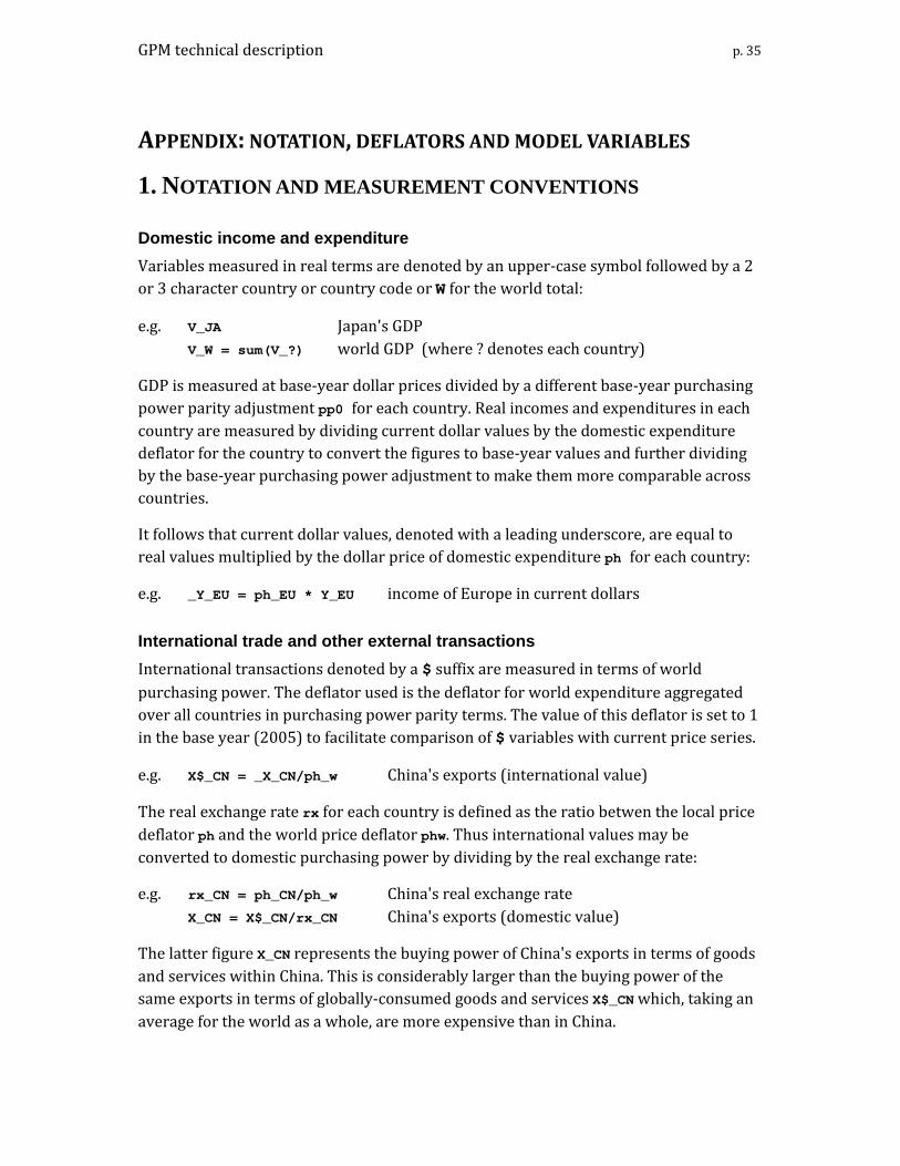
GPM technical description p. 35
APPENDIX: NOTATION, DEFLATORS AND MODEL VARIABLES
1. NOTATION AND MEASUREMENT CONVENTIONS
Domestic income and expenditure Variables measured in real terms are denoted by an upper‐case symbol followed by a 2 or 3 character country or country code or W for the world total:
e.g. V_JA Japan's GDP V_W = sum(V_?) world GDP (where ? denotes each country)
GDP is measured at base‐year dollar prices divided by a different base‐year purchasing power parity adjustment pp0 for each country. Real incomes and expenditures in each country are measured by dividing current dollar values by the domestic expenditure deflator for the country to convert the figures to base‐year values and further dividing by the base‐year purchasing power adjustment to make them more comparable across countries.
It follows that current dollar values, denoted with a leading underscore, are equal to real values multiplied by the dollar price of domestic expenditure ph for each country:
e.g. _Y_EU = ph_EU * Y_EU income of Europe in current dollars
International trade and other external transactions International transactions denoted by a $ suffix are measured in terms of world purchasing power. The deflator used is the deflator for world expenditure aggregated over all countries in purchasing power parity terms. The value of this deflator is set to 1 in the base year (2005) to facilitate comparison of $ variables with current price series.
e.g. X$_CN = _X_CN/ph_w China's exports (international value)
The real exchange rate rx for each country is defined as the ratio betwen the local price deflator ph and the world price deflator phw. Thus international values may be converted to domestic purchasing power by dividing by the real exchange rate:
e.g. rx_CN = ph_CN/ph_w China's real exchange rate X_CN = X$_CN/rx_CN China's exports (domestic value)
The latter figure X_CN represents the buying power of China's exports in terms of goods and services within China. This is considerably larger than the buying power of the same exports in terms of globally‐consumed goods and services X$_CN which, taking an average for the world as a whole, are more expensive than in China.
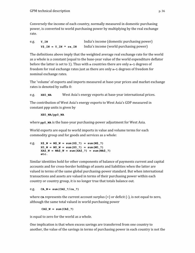
GPM technical description p. 36
Conversely the income of each country, normally measured in domestic purchasing power, is converted to world purchasing power by multiplying by the real exchange rate.
e.g. Y_IN India's income (domestic purchasing power) Y$_IN = Y_IN * rx_IN India's income (world purchasing power)
The definitions above imply that the weighted average real exchange rate for the world as a whole is a constant (equal to the base‐year value of the world expenditure deflator before the latter is set to 1). Thus with n countries there are only n-1 degrees of freedom for real exchange rates just as there are only n-1 degrees of freedom for nominal exchange rates.
The 'volume' of exports and imports measured at base‐year prices and market exchange rates is denoted by suffix 0:
e.g. XE0_WA West Asia's energy exports at base‐year international prices.
The contribution of West Asia's energy exports to West Asia's GDP measured in constant ppp units is given by
XE0_WA/pp0_WA
where pp0_WA is the base‐year purchasing‐power adjustment for West Asia.
World exports are equal to world imports in value and volume terms for each commodity group and for goods and services as a whole:
e.g. X$_W = M$_W = sum(X$_?) = sum(M$_?) X0_W = M0_W = sum(X0_?) = sum(M0_?) XA$_W = MA$_W = sum(XA$_?) = sum(MA$_?) etc.
Similar identities hold for other components of balance of payments current and capital accounts and for cross‐border holdings of assets and liabilities when the latter are valued in terms of the same global purchasing‐power standard. But when international transactions and assets are valued in terms of their purchasing power within each country or country group, it is no longer true that totals balance out.
e.g. CA_W = sum(CA$_?/rx_?)
where CA represents the current account surplus (+) or deficit (‐), is not equal to zero, although the same total valued in world purchasing power
CA$_W = sum(CA$_?)
is equal to zero for the world as a whole.
One implication is that when excess savings are transferred from one country to another, the value of the savings in terms of purchasing power in each country is not the

GPM technical description p. 37
same. Thus if savings are transferred from a low‐income country where goods and services are cheap to a high‐income country where goods and services are more expensive, the volume of expenditure foregone in the low‐income country is greater than the volume of additional expenditure in the high‐income country. Evidently the reverse is the case when savings are transferred from high‐income to low‐income countries.
Prices and rates Prices, rates of inflation, interest rates and exchange rates are denoted with lower‐case symbols:
e.g. pvi_EU Europe's average local currency cost inflation rate (% p.a.) is_EU Europe's average local ccy. short‐term interest rate (% p.a.) irs_w world average 'real' short‐term interest rate (% p.a.)
Values for a country group are weighted averages of values for countries in the group.30
Assets and liabilities Assets and liabilities at end year are converted from current dollars to real values by dividing by the period expenditure deflator (the same deflator that is used for income and expenditure in the period). The real value of assets and liabilities may rise or fall from year to year on account of changes in their price or nominal value in the currency in which they are quoted or denominated, as well as changes in the dollar exchange rate for that currency and changes in the purchasing power of the dollar as measured by the domestic or world expenditure deflator.
Holding gains measured in real terms are denoted with the prefix H and cash flows (net acquisition or sale) of assets are denoted with the prefix I. For example
AGF_US US government investment in banks HAGF_US holding gains or losses on US government investment in banks IAGF_US net cash proceeds of US government transactions in bank liabilities
The relationship between stocks and flows may be written as
AGF_US = AGF_US(-1) + HAGF_US + IAGF_US
30 Expenditure weights are used to average domestic price inflation and nominal interest rates across countries within a country group. GDP weights are used to average cost inflation. Implicitly, group‐level real interest rates are expenditure‐weighted averages of rates in each country.

GPM technical description p. 38
The valuation of assets and liabilities brought forward from the previous year is represented by a variable whose name begins with rp.
e.g. LG_IN India government debt at end‐year rpfa_IN valuation for prior-year assets LG_IN(-1)*rpfa_IN value of debt brought forward ILG_IN proceeds of debt issues less redemptions
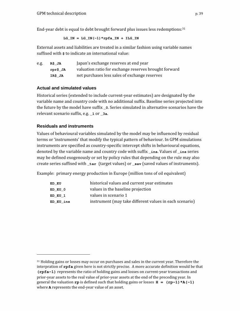
GPM technical description p. 39
End‐year debt is equal to debt brought forward plus issues less redemptions:31
LG_IN = LG_IN(-1)*rpfa_IN + ILG_IN
External assets and liabilities are treated in a similar fashion using variable names suffixed with $ to indicate an international value:
e.g. R$_JA Japan's exchange reserves at end year rpr$_JA valuation ratio for exchange reserves brought forward IR$_JA net purchases less sales of exchange reserves
Actual and simulated values Historical series (extended to include current‐year estimates) are designated by the variable name and country code with no additional suffix. Baseline series projected into the future by the model have suffix _0. Series simulated in alternative scenarios have the relevant scenario suffix, e.g. _1 or _3a.
Residuals and instruments Values of behavioural variables simulated by the model may be influenced by residual terms or ‘instruments’ that modify the typical pattern of behaviour. In GPM simulations instruments are specified as country‐specific intercept shifts in behavioural equations, denoted by the variable name and country code with suffix _ins. Values of _ins series may be defined exogenously or set by policy rules that depending on the rule may also create series suffixed with _tar (target values) or _sav (saved values of instruments).
Example: primary energy production in Europe (million tons of oil equivalent)
ED_EU historical values and current year estimates ED_EU_0 values in the baseline projection ED_EU_1 values in scenario 1 ED_EU_ins instrument (may take different values in each scenario)
31 Holding gains or losses may occur on purchases and sales in the current year. Therefore the interpration of rpfa given here is not strictly precise. A more accurate definition would be that (rpfa-1) represents the ratio of holding gains and losses on current‐year transactions and prior‐year assets to the real value of prior‐year assets at the end of the preceding year. In general the valuation rp is defined such that holding gains or losses H = (rp-1)*A(-1) where A represents the end‐year value of an asset.

GPM technical description p. 40
2. REAL VALUES, VOLUMES AND PRICE DEFLATORS
Series Description Source or formula 1. Expenditure and expenditure deflators APT GDP in current dollars databank
APT1 GDP at current purchasing power parity databank
AXD domestic expenditure in current dollars databank
AXD0 domestic expenditure at base-year prices databank
PXA index of world prices for primary commodities databank
PXE index of world price of oil databank
Model variables - country level pp0 base-year purchasing power parity adjustment APT(base)/APT1(base)
H domestic expenditure, base-year purchasing power AXD0/pp0
ph domestic expenditure deflator AXD/H = AXD.pp0/AXD0
_H domestic expenditure in current dollars H.ph
Model variables – global HW world expenditure, base-year purchasing power sum(H)
pp0w base-year PPP adjustment sum(AXD(base))/sum(H(base))
phw world expenditure deflator sum(AXD)/(pp0w.sum(H))
paw world price of primary commodities, base-year world value PXA/phw
pew world price of oil, base-year world value PXE/phw
2. Real exchange rate, current account, national income and GDP APT0 GDP at base-year prices databank
AXX exports in current dollars databank
AXX0 exports at base-year prices databank
AXM imports in current dollars databank
AXM0 imports at base-year prices databank
BCA current account in dollars databank
Model variables - country level rx real exchange rate ph/phw
CA$ current account, base-year world value BCA/phw
TB$ trade balance, base-year world value (AXX-AXM)/phw
TB0 net exports at base-year prices TB0 = AXX0-AXM0
BIT$ balance on income and transfers, base-year world value CA$ - TB$
Y national income, base-year purchasing power (AXD+BCA)/ph
V GDP volume, base-year purchasing parity APT0/pp0
VV expenditure on GDP H + TB$/rx
tt terms of trade effect (ratio of GDP value to volume)
(H + TB$/rx)/V

GPM technical description p. 41
Series Description Source or formula Country level theorems T1 Income, domestic expenditure and current a/c H = C + IP + IV + G
Y = H + CA$/rx
= H + TB$/rx + BIT$/rx
T2 GDP, expenditure and net export volume V = H + TB0/pp0
VV = H + TB$/rx
T3 Income, GDP and the terms of trade Y = V.tt + BIT$/rx
Theorem - world level T4 Weighted average real exchange rate sum(H.rx)/sum(H) = pp0w
Proof H.rx = H.ph/ph_w
= AXD.pp0_w.sum(H)/sum(AXD)
sum(H.rx) = pp0_w.sum(H)
definition of rx
defns of ph and ph_w
sum over countries
3. Inflation and nominal exchange rate appreciation APT3 GDP in domestic currency units (databank - internal)
AXD3 domestic expenditure in domestic currency units (databank - internal)
PPT cost of constant dollar GDP in domestic currency units APT3/APT0
PXD price of constant dollar domestic expenditure in domestic currency units
AXD3/AXD0
RXN exchange rate - dollars per domestic currency unit APT/APT3 = AXD/AXD3
Model variables - country level pvi domestic cost inflation (% p.a.) 100(PPT/PPT(-1) – 1)
pi domestic price inflation (% p.a.) 100(PXD/PXD(-1) – 1)
rxna nominal exchange rate appreciation (% p.a.) 100(RXN/RXN(-1) – 1)
Country level theorems T5 Price inflation, cost inflation and the terms of trade (1+pi/100) = (1+pvi/100)
.tt(-1)/tt
Proof PXD/PPT = (AXD/APT).(APT0/AXD0)
= ph.V /(AXD+AXX-AXM)
= V/(H + TB$/rx) = 1/tt
defns of PPT, PXD and RXN
defns of ph,V and APT
defns of H, rx and tt
T6 Nominal exchange rate appreciation (1+rxna/100) = (ph/ph(-1)
/(1+pi/100)
Proof RXN.PXD = AXD/AXD0
= ph/pp0
defns of RXN, PXD
definition of ph
Theorem - world level T7 Movement of global dollar prices relative to US prices and real exchange rate movements
ph_w = ph_w(-1).
(1+pi_us/100).
rx_us(-1)/rx_us

GPM technical description p. 42
3. VARIABLES AND IDENTITIES Variables with no suffix represent domestic purchasing power values, variables suffixed with $ are measured in terms of world purchasing power, and variables suffixed with 0 denote volumes or quantities measured at base‐year prices and exchange rates. Variables suffixed with _W represent world indexes or totals.32
Model variables Symbol Name Units Exogenous, behavioural or determined by identity AGF Bank deposits and capital held by
government at end year $m AGF = NGI + max(NGF,0)
AX$ External assets at end year $m AX$ = R$ + AXO$ AXO$ Other external assets at end year
(adjusted) $m AXO$ = AXO$U.AXO$_W / AXO$U_W
AXO$U Other external assets at end year (unadjusted)
$m AXO$U = NXI$ + max(NXF$U,0)
BA$ Net exports of primary commodities
$m BA$ = XA$ - MA$
BA0 Net exports of primary commodities at base-year prices (adjusted)
$m BA0 = XA0 - MA0
BA0U Net exports of primary commodities at base-year prices (unadjusted)
$m behavioural [structural policy]
BE$ Net exports of fuels $m BE$ = XE$- ME$ BE0 Net exports of fuels at base-year
prices $m BE0 = XE0 - ME0
BIT$ Net income and transfers from abroad
$m BIT$ = XIT$ - MIT$
BIT$U Net income and transfers from abroad (unadjusted)
$m behavioural [structural policy]
BM$ Net exports of manufactures $m BM$ = XM$ - MM$ BM0 Net exports of manufactures at
base-year prices $m BM0 = XM0 - MM0
BS$ Net exports of services (adjusted) $m BS$ = XS$ - MS$ BS0 Net exports of services at base-year
prices $m BS0 = XS0 - MS0
BS$U Net exports of services (unadjusted)
$m behavioural [structural policy]
C Consumers expenditure $m C = YP – SP CA$ Current account balance of
payments $m CA$ = TB$ + BIT$
CO2 CO2 emissions m tons behavioural [energy policy] DNNVF Natural increase in female
population 25+ millions exogenous
DNNVM Natural increase in male population 25+
millions exogenous
32 Most variables are also available in current US dollars (variable name prefixed by _).

GPM technical description p. 43
Symbol Name Units Exogenous, behavioural or determined by identity DNNYF Natural increase in female
population 15-24 millions exogenous
DNNYM Natural increase in male population 15-24
millions exogenous
DP Bank deposits at end-year $m DP = NFI + max(NFF,0) EB Energy balance mtoe EB = EX – EM ED Energy demand mtoe behavioural [structural policy] ei Increase in average earnings % p.a. behavioural [incomes policy] EM Primary energy imports mtoe behavioural [trade policy] EPC Primary carbon energy production mtoe behavioural [energy policy] EPN Primary non-carbon energy
production mtoe behavioural [energy policy]
EX Primary energy exports mtoe EX = EPC + EPN + EM – ED G Government expenditure $m behavioural [fiscal policy] GSS Government service standard index 100*(G/(NCP+NYF+NYM+NOP))/YN H Domestic expenditure $m H = C + IP + IV + G HAGF Holding gain or loss on
government investment in banks $m HAGF = R(-1).rpr$/rx + (LN(-1)+
LGF(-1)–DP(-1)).rpfa – AGF(-1)- lnbail.LN(-1).wln.rpfa
HAXO Holding gain on other external assets
$m HAXO = AXO$/rx - AXO$(-1)/rx(-1) – IAXO$/rx
HDP Holding gain or loss on other sectors' investment and deposits with banks
$m HDP = DP - DP(-1) – IDP
HKP Holding gain or loss on capital stock at end year
$m HKP = KP - KP(-1) - KI + KI(-1)
HLGO Holding gain or loss on other government debt
$m HLGO = LGO - LGO(-1) – ILGO
HLN Holding gain or loss on bank lending
$m HLN = LN - LN(-1) – ILN
HLX Holding gain or loss on external liabilities
$m HLX = LX$/rx - LX$(-1)/rx(-1) - ILX$/rx
HWP Holding gain or loss on private wealth
$m HWP = HKP + HDP - HLN + HLGO + HAXO - HLX
IAG Government asset transactions $m IAG = IAGF + IAGO IAGF Government injections to banks $m IAGF = AGF - AGF(-1) – HAGF IAGO Other government asset
transactions $m behavioural [financial policy]
IAXO$ Other external capital outflow $m IAXO$ = ILX$ - IR$ + CA$ IDP Acquisition of bank deposits $m IDP = ILN – ILGO + IAGO – (IAXO$
- ILX$) / rx + NLP
ILG Net issues of government debt $m ILG = IAG – NLG ILGF Acquisition of government debt by
banks $m ILGF = ILG – ILGO
ILGO Non-bank acquisition of government debt
$m ILGO = LGO - LGO(-1).rpfa
ILN Net lending by banks to non-government sectors
$m ILN = LN - LN(-1).rpfa.(1-wln)
ILX$ Other external borrowing $m ILX$ = LX$ - LX$(-1).rplx$ im Bond rate % p.a. behavioural [confidence]

GPM technical description p. 44
Symbol Name Units Exogenous, behavioural or determined by identity IP Private investment $m behavioural [confidence] IR$ Net acquisition of exchange
reserves $m IR$ = R$ - R$(-1).rpr$
irm Real bond rate % p.a. irm= 100((1+im/100)/(1+pi/100)-1) irs Short term interest rate % p.a. irs= 100((1+is/100)/(1+pi/100)-1) is Short-term interest rate % p.a. behavioural [monetary policy] IV Change in inventories $m behavioural [confidence] KI Produced capital stock at end year $m KI = (1-rdp)*KI(-1) + IP + IV KID Capital consumption $m KID = rdp KI(-1) KP Value of capital at end year $m KP = pkp.KI LG Government debt at end year $m LG = AGF – NGF LGF Government debt held by banks at
end year $m LGF = LG - LGO
LGO Non-bank holdings of government debt at end year
$m behavioural [monetary policy]
LN Bank loans outstanding at end year $m LN = DP - NFF lnbail Government bail-out losses as
proportion of abnormal loan write-offs by banks
ratio constant [assumption]
lpa Domestic impact of world price of primary commodities
log lpa = 0.3 log(pa_w/rx) + 0.7 lpa(-1)
lped Demand impact of user price of energy
log lped = 0.3 log(ped*rx/(pepmax-400*pe_w)) + 0.7 lped(-1)
lpep Production impact of producer price of carbon energy
log lpep = 0.15 log(pep*rx/(pepmax-400*pe_w)) + 0.85 lpep(-1)
lpepc Production impact of producer price of non-carbon energy
log lpepc = 0.05 log(pepc*rx/(pepmax-400*pe_w)) + 0.95 lpepc(-1)
LX$ External liabilities at end year $m LX$ = AXO$U - NXF$U M$ Imports of goods and services $m M$ = MA$ + ME$ + MM$ + MS$ M0 Import of goods and services at
base-year prices $m M0 = MA0 + ME0 + MM0 + MS0
MA$ Imports of primary commodities $m behavioural [volume, prices] MA0 Imports of primary commodities at
base-year prices (adjusted) $m MA0 = MA0U XA0_W/sum(MA0U)
MA0U Imports of primary commodities at base-year prices (unadjusted)
$m MA0U = XA0 – BA0U
ME$ Imports of energy products $m behavioural [volume, prices] ME0 Imports of energy products at base-
year (adjusted) $m ME0 = ME0U XE0_W/sum(ME0U)
ME0U Imports of energy products at base-year (unadjusted)
$m behavioural [product mix]
mh Import content of domestic expenditure
ratio mh = M0/(pp0.H + vx.X0)
MIT$ Income paid abroad $m MIT$ = XIT$U - BIT$U MM$ Imports of manufactures $m behavioural [trade policy] MM0 Imports of manufactures at base-
year prices (adjusted) $m MM0 = MM0U XM0_W/sum(MM0U)
MM0U
Imports of manufactures at base-year prices (unadjusted)
$m behavioural [prices, value]
MS$ Imports of services $m behavioural [trade policy] MS0 Imports of services at base-year $m MS0 = MS0U XS0_W/sum(MS0U)

GPM technical description p. 45
Symbol Name Units Exogenous, behavioural or determined by identity prices (adjusted)
MS0U Imports of services at base-year prices (unadjusted)
$m behavioural [prices, value]
mu profit markup % behavioural [incomes policy]
N Total population millions N = NCP + NP NCP Child population millions exogenous NE Employment millions NE = NEF + NEM NEA Employment in agriculture millions NEA = NEAF + NEAM NEAF Female employment in agriculture millions behavioural [labour market] NEAM Male employment in agriculture millions behavioural [labour market] NEEF Female employees millions behavioural [labour market] NEEM Male employees millions behavioural [labour market] NEF Female employment millions NEF = NEYF + NEVF NEI Employment in industry millions NEI = NEIF + NEIM NEIF Female employment in industry millions behavioural [labour market] NEIM Male employment in industry millions behavioural [labour market] NEM Male employment millions NEM = NEYM + NEVM NEN Non-agricultural employment millions NEN = NENF + NENM NENF Female non-agric employment millions NENF = NEF - NEAF NENM Male non-agricultural employment millions NENM = NEM - NEAM NES Employment in services millions NES = NESF + NESM NESF Female employment in services millions NESF = NENF - NEIF NESM Male employment in services millions NESM = NENM - NEIM NEVF Female employment 25+ millions NEVF = NLVF – NUVF NEVM Male employment 25+ millions NEVM = NLVM – NUVM NEYF Female employment 15-24 millions NEYF = NLYF – NUYF NEYM Male employment 15-24 millions NEYM = NLYM – NUYM NFF Bank deposits less loans at end
year $m NFF = R$/rx + LGF - AGF
NFI Covered bank lending $m behavioural [confidence] NGF Government investment and
deposits with banks less outstanding debt at end year
$m NGF = NLG + AGF(-1) + HAGF – IAGO – LGO(-1).rplgo - LGF(-1).rpfa
NGI Covered government debt $m behavioural [monetary policy] NIM Net migration (adjusted) millions NIM = NIMU + NIMU_W*(NIMU -
abs(NIMU))/(sum(abs(NIMU)) – NIMU_W)
NIMU Net migration (unadjusted) millions behavioural [labour market] NIT$ Net income and transfers
(adjusted) $m NIT$ = min(XIT$, MIT$)
NIT$U Net income and transfers (unadjusted)
$m behavioural [external policy]
NL Total labour force millions NL = NLF + NLM NLF Female labour force millions NLF = NLYF + NLVF NLM Male labour force millions NLM = NLYM + NLVM NLG Government net lending $m NLG = YG – G NLP Private net lending $m NLP = SP - IP – IV NLVF Female labour force 25+ millions behavioural [labour market]
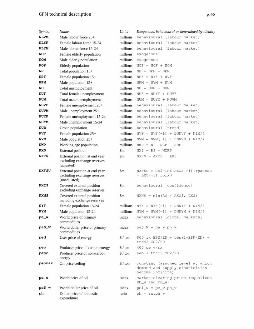
GPM technical description p. 46
Symbol Name Units Exogenous, behavioural or determined by identity NLVM Male labour force 25+ millions behavioural [labour market] NLYF Female labour force 15-24 millions behavioural [labour market] NLYM Male labour force 15-24 millions behavioural [labour market] NOF Female elderly population millions exogenous NOM Male elderly population millions exogenous NOP Elderly population millions NOP = NOF + NOM NP Total population 15+ millions NP = NPF + NPM NPF Female population 15+ millions NPF = NYF + NVF NPM Male population 15+ millions NPM = NYM + NVM NU Total unemployment millions NU = NUF + NUM NUF Total female unemployment millions NUF = NUYF + NUVF NUM Total male unemployment millions NUM = NUYM + NUVM NUVF Female unemployment 25+ millions behavioural [labour market] NUVM Male unemployment 25+ millions behavioural [labour market] NUYF Female unemployment 15-24 millions behavioural [labour market] NUYM Male unemployment 15-24 millions behavioural [labour market] NUR Urban population millions behavioural [trend] NVF Female population 25+ millions NVF = NVF(-1) + DNNVF + NIM/4 NVM Male population 25+ millions NVM = NVM(-1) + DNNVM + NIM/4 NWP Working age population millions NWP = N - NCP - NOP NX$ External position $m NX$ = R$ + NXF$ NXF$ External position at end year
excluding exchange reserves (adjusted)
$m NXF$ = AXO$ - LX$
NXF$U External position at end year excluding exchange reserves (unadjusted)
$m NXF$U = CA$-IR$+AXO$(-1).rpaxo$u - LX$(-1).rplx$
NXI$ Covered external position excluding exchange reserves
$m behavioural [confidence]
NXN$ Covered external position including exchange reserves
$m NXN$ = min(R$ + AXO$, LX$)
NYF Female population 15-24 millions NYF = NYF(-1) + DNNYF + NIM/4 NYM Male population 15-24 millions NYM = NYM(-1) + DNNYM + NIM/4 pa_w World price of primary
commodities index behavioural [global markets]
pa$_W World dollar price of primary commodities
index pa$_W = pa_w.ph_w
ped User price of energy $ / ton 800 rx EPN/ED + pep(1-EPN/ED) + ttco2 CO2/ED
pep Producer price of carbon energy $ / ton 400 pe_w/rx pepc Producer price of non-carbon
energy $ / ton pep + ttco2 CO2/ED
pepmax Oil price ceiling $ / ton constant (assumed level at which demand and supply elasticities become infinite)
pe_w World price of oil index market-clearing price (equalizes ED_W and EP_W)
pe$_w World dollar price of oil index pe$_w = pe_w.ph_w ph
Dollar price of domestic expenditure
ratio ph = rx.ph_w

GPM technical description p. 47
Symbol Name Units Exogenous, behavioural or determined by identity phd
Domestic price index index phd = phd(-1)(1+pi/100)
ph_w World dollar price of expenditure ratio ph_w = ph_w(-1).(1+pi_us/100). rx_us(-1)/rx_us
pi Domestic currency price inflation % p.a. pi = 100((1+pvi/100).tt(-1)/tt-1) pi$ Dollar price inflation
pi$ = 100*(ph/ph(-1)-1)
pi_w World average domestic currency price inflation
% p.a. pi_w = sum(pi.H)/H_W
pi$_w World dollar price inflation % p.a. pi$_w = 100 (ph_w/ph_w(-1) - 1) pkp Price of capital (ratio of value of
capital including land to produced capital stock)
deflator behavioural [confidence]
pmm Price of imports of manufactures deflator ppm = MM$ / MM0 pmm0 Average supplier price for imports
of manufactures deflator ppm0 = 1/sum(suppliers:
sxm*(XM0/XM$)) pp0 Base-year ppp adjustment ratio constant pp0_w World base-year ppp adjustment ratio constant pvd Domestic cost index index pvd = pvd(-1)(1+pvi/100) pvi Domestic cost inflation % p.a. pvi = 100((1+ei/100)((1+mu/100)/
(1+mu(-1)/100))((1+rtx/100)/ (1+rtx(-1)/100))(V(-1)*NE/ (V*NE(-1)))-1)
pxm Price of exports of manufactures index pxm = XM$ / XM0 R$ Exchange reserves at end year $m behavioural (monetary policy) ralx$ External asset/liability ratio % ralx$ = 100*AX$/LX$ rax External asset ratio % rax = 100*AX$/(RX*DP) rax0 Non-reserve asset ratio % rax0 = 100*AX0$/(RX*DP) rlx External liability ratio % rlx = 100*LX$/(RX*DP) rmx$ Reserves as % of annual imports % rmx$ = 100*R$/M$ rpaxo$ Valuation ratio for other external
assets brought forward (adjusted) ratio rpaxo$ = (AXO$-IAXO$)/AXO$(-1)
rpaxo$u Valuation ratio for other external assets brought forward (unadjusted)
$m behavioural [price movements]
rpfa Valuation ratio for domestic financial assets brought forward
ratio rpfa = 1/(1+spvi) [assumption]
rpkp Valuation ratio for capital stock brought forward
ratio rpkp = pkp/pkp(-1)
rplgo Valuation ratio for non-bank holdings of government debt brought forward
ratio rplgo = slgx.ph(-1)/ph + (1-slgx).rpfa
rplx$ Valuation ratio for external liabilities brought forward
ratio behavioural [price movements]
rpr$ Valuation ratio for exchange reserves brought forward
ratio behavioural [price movements]
rtx Indirect tax markup % p.a. behavioural [fiscal policy] rx Real exchange rate (adjusted) ratio rx = rxu / rxadj rxd Nominal exchange rate index rxd = rxd(-1)(1+rxna/100) rxna Nominal exchange rate
appreciation % p.a. rxna = 100((ph/ph(-1))
/(1+pi/100)-1)

GPM technical description p. 48
Symbol Name Units Exogenous, behavioural or determined by identity rxu Real exchange rate (unadjusted) ratio behavioural [monetary policy,
confidence] slgx Proportion of government debt
financed in foreign currency ratio slgx = 1 – log(1+YR)/2
[assumption] SP Private saving $m behavioural [confidence] SPV Private saving as % of GDP % p.a. SPV = 100*SP/VV spvi Inflation indicator
log spvi = log(-0.718 +
3.436(1+pvi/100) /(2+pvi/100)) sxm Market share of exports of
manufactures in imports of each destination (adjusted)
ratio sxm = sxmu / sum(sxmu)
sxmm Percent share of world exports of manufactures
% p.a. sxmm = 100 XM$ / MM$_W
sxmu Market share of exports of manufactures in imports of each destination (unadjusted)
ratio behavioural [trade policy]
TB$ Trade balance $m TB$ = X$ - M$ TB0 Trade balance at base year prices $m TB0 = X0 – M0 tt Terms of trade effect ratio tt = (H+TB$/rx) /(H+TB0/pp0) ttco2 Carbon tax $/ton exogenous [energy policy] ucx$ Real unit cost of exports index ucx$ = mh*vx*M$/M0+(1-
mh*vx)*rx/pp0 ulc$ Unit labour cost index ulc$ = rx*VVEM*pp0/V0 uva$ Unit factor cost index uva$ = RX*(VVEM+VVPR)*pp0/V0 V0 GDP at base-year exchange rates $m V0 = V.pp0 V GDP volume $m V = H + TB0/pp0 VGA Productivity gap in agriculture % VGA = 100*(NEA/NE-WA/VV)/(1-
NEA/NE) VNE GDP per employed person $ VNE = V / NE VT Productive capacity $m VT = 1.05 movav(V,6).
(V/V(-6))^0.3 VV Domestic purchasing power of
GDP $m VV = H + TB$/rx
VV$ External purchasing power of GDP $m VV$ = H*rx + TB$ VVA GDP in agriculture $m behavioural (demand/supply) VVE GDP in extraction and utilities $m behavioural (demand/supply) VVEE Compensation of employees $m behavioural (labour market) VVEM Labour and mixed income $m VVEM = VV - VVPR - VVTX VVI GDP in industry $m behavioural (demand/supply) VVPR Profits and rent $m VVPR = mu(VV - VVTX)/(100 + mu) VVN GDP per capita $ VVN = VV/N VVS GDP in services $m VVS = VV - VVA - VVE - VVI VVT Capacity utilization % p.a. VVT = 100*(V/VT - 1) VVTX Indirect taxes less subsidies $m VVTX = rtx VV / (100 + rtx) vx Import content of exports relative
to import content of domestic expenditure
ratio vx = 2 + (X0-M0)/(pp0.V) [assumption]
wln Write-off rate for bank loans % p.a. exogenous [confidence] WLNA Lagged loan write-offs $m WLNA = 0.8 LN(-1).wln.rpfa +
0.2 WLNA(-1)

GPM technical description p. 49
Symbol Name Units Exogenous, behavioural or determined by identity WP Private wealth at end-year ratio WP = KP + LGO + NFF + NXF$ / rx X$ Exports of goods and services $m X$ = XA$ + XE$ + XM$ + XS$ X0 Exports of goods and services at
base-year prices $m X0 = XA0 + XE0 + XM0 + XS0
XA$ Exports of primary commodities (adjusted)
$m XA$ = XA$U MA$_W/sum(XA$U)
XA0 Exports of primary commodities at base-year prices
$m behavioural [trade policy]
XA$U Exports of primary commodities (unadjusted)
$m behavioural [price behaviour]
XE$ Exports of energy products $m XE$ = XE$U ME$_W/sum(XE$U) XE$U Exports of energy products
(unadjusted) $m behavioural [price behaviour]
XE0 Exports of energy products at base- year prices
$m behavioural [trade policy]
XIT$ Income and transfers from abroad (adjusted)
$m XIT$ = XIT$U.MIT$_W/XITU$_W
XIT$U
Income and transfers from abroad (unadjusted)
$m XIT$U = NIT$U + max(BIT$U, 0)
XM$ Exports of manufactures $m XM$ = sum(partners: sxm MM$) XM0 Exports of manufactures at base-
year prices $m behavioural [price behaviour]
XS$ Exports of services (adjusted) $m XS$ = XS$U MS$_W/sum(XS$U) XS0 Exports of services at base-year
prices $m behavioural [price behaviour]
XS$U Exports of services (unadjusted) $m XS$U = BS$U + MS$ Y National income (domestic
purchasing power) $m Y = H + CA$/rx
Y$ National income (international purchasing power)
$m Y$ = Y / rx
YG Government net income $m YG = YGD + VVTX YGD Direct taxes less transfers $m behavioural [fiscal policy] YN Income per capita $ pp YN = Y / N YN$ Income per capita at market rates $ wpp YN$ = Y$ / N YP Private disposable income $m YP = Y – YG YPN Private income net of capital
consumption $m YP – KID
YR Relative income per capita Ratio YR = YN / YN_W
Additional variables for policy evaluation Variables listed below are calculated after solution of the core model. In addition to these variables, many growth rates and ratios are computed for display in graphs.
Symbol Name Units Exogenous, behavioural or determined by identity
GY Population-weighted Gini coefficient for distribution of income between countries
Index computed on countries in ascending sequence by income per capita
NER Employment rate % NER = 100 NE / NP NUL Unemployment rate % NUL = 100 NU / NL
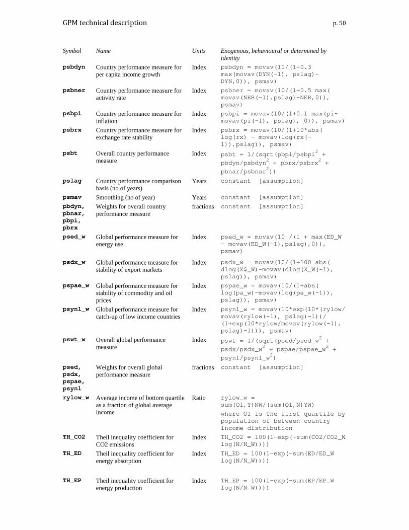
GPM technical description p. 50
Symbol Name Units Exogenous, behavioural or determined by identity
psbdyn Country performance measure for per capita income growth
Index psbdyn = movav(10/(1+0.3 max(movav(DYN(-1), pslag)-DYN,0)), psmav)
psbner Country performance measure for activity rate
Index psbner = movav(10/(1+0.5 max( movav(NER(-1),pslag)-NER,0)), psmav)
psbpi Country performance measure for inflation
Index psbpi = movav(10/(1+0.1 max(pi-movav(pi(-1), pslag), 0)), psmav)
psbrx Country performance measure for exchange rate stability
Index psbrx = movav(10/(1+10*abs( log(rx) - movav(log(rx(-1)),pslag)), psmav)
psbt Overall country performance measure
Index psbt = 1/(sqrt(pbpi/psbpi2 + pbdyn/psbdyn2 + pbrx/psbrx2 + pbnar/psbnar2))
pslag Country performance comparison basis (no of years)
Years constant [assumption]
psmav Smoothing (no of year) Years constant [assumption] pbdyn, pbnar, pbpi, pbrx
Weights for overall country performance measure
fractions constant [assumption]
psed_w Global performance measure for energy use
Index psed_w = movav(10 /(1 + max(ED_W - movav(ED_W(-1),pslag),0)), psmav)
psdx_w Global performance measure for stability of export markets
Index psdx_w = movav(10/(1+100 abs( dlog(X$_W)-movav(dlog(X_W(-1), pslag)), psmav)
pspae_w Global performance measure for stability of commodity and oil prices
Index pspae_w = movav(10/(1+abs( log(pa_w)-movav(log(pa_w(-1)), pslag)), psmav)
psynl_w Global performance measure for catch-up of low income countries
Index psynl_w = movav(10*exp(10*(rylow/ movav(rylow(-1), pslag)-1))/ (1+exp(10*rylow/movav(rylow(-1), pslag)-1))), psmav)
pswt_w Overall global performance measure
Index pswt = 1/(sqrt(psed/psed_w2 + psdx/psdx_w2 + pspae/pspae_w2 + psynl/psynl_w2)
psed, psdx, pspae, psynl
Weights for overall global performance measure
fractions constant [assumption]
rylow_w Average income of bottom quartile as a fraction of global average income
Ratio rylow_w = sum(Q1,Y)NW/(sum(Q1,N)YW) where Q1 is the first quartile by population of between-country income distribution
TH_CO2 Theil inequality coefficient for CO2 emissions
Index TH_CO2 = 100(1-exp(-sum(CO2/CO2_W log(N/N_W))))
TH_ED
Theil inequality coefficient for energy absorption
Index TH_ED = 100(1-exp(-sum(ED/ED_W log(N/N_W))))
TH_EP Theil inequality coefficient for energy production
Index TH_EP = 100(1-exp(-sum(EP/EP_W log(N/N_W))))

GPM technical description p. 51
Symbol Name Units Exogenous, behavioural or determined by identity
TH_G Theil inequality coefficient for government expenditure
Index TH_G = 100(1-exp(-sum(G/G_W log(N/N_W))))
TH_XM$ Theil inequality coefficient for exports of manufactures
Index TH_XM$ = 100(1-exp(-sum(XM$/XM$_W log(N/N_W))))
TH_XS$ Theil inequality coefficient for exports of services
Index TH_XS$ = 100(1-exp(-sum(XS$/XS$_W log(N/N_W))))
TH_Y Theil inequality coefficient for income
Index TH_Y = 100(1-exp(-sum(Y/Y_W log(N/N_W))))