The UCM Procedure
119
SAS/ETS ® 13.2 User’s Guide The UCM Procedure
Transcript of The UCM Procedure

SAS/ETS® 13.2 User’s GuideThe UCM Procedure

This document is an individual chapter from SAS/ETS® 13.2 User’s Guide.
The correct bibliographic citation for the complete manual is as follows: SAS Institute Inc. 2014. SAS/ETS® 13.2 User’s Guide.Cary, NC: SAS Institute Inc.
Copyright © 2014, SAS Institute Inc., Cary, NC, USA
All rights reserved. Produced in the United States of America.
For a hard-copy book: No part of this publication may be reproduced, stored in a retrieval system, or transmitted, in any form or byany means, electronic, mechanical, photocopying, or otherwise, without the prior written permission of the publisher, SAS InstituteInc.
For a Web download or e-book: Your use of this publication shall be governed by the terms established by the vendor at the timeyou acquire this publication.
The scanning, uploading, and distribution of this book via the Internet or any other means without the permission of the publisher isillegal and punishable by law. Please purchase only authorized electronic editions and do not participate in or encourage electronicpiracy of copyrighted materials. Your support of others’ rights is appreciated.
U.S. Government License Rights; Restricted Rights: The Software and its documentation is commercial computer softwaredeveloped at private expense and is provided with RESTRICTED RIGHTS to the United States Government. Use, duplication ordisclosure of the Software by the United States Government is subject to the license terms of this Agreement pursuant to, asapplicable, FAR 12.212, DFAR 227.7202-1(a), DFAR 227.7202-3(a) and DFAR 227.7202-4 and, to the extent required under U.S.federal law, the minimum restricted rights as set out in FAR 52.227-19 (DEC 2007). If FAR 52.227-19 is applicable, this provisionserves as notice under clause (c) thereof and no other notice is required to be affixed to the Software or documentation. TheGovernment’s rights in Software and documentation shall be only those set forth in this Agreement.
SAS Institute Inc., SAS Campus Drive, Cary, North Carolina 27513.
August 2014
SAS provides a complete selection of books and electronic products to help customers use SAS® software to its fullest potential. Formore information about our offerings, visit support.sas.com/bookstore or call 1-800-727-3228.
SAS® and all other SAS Institute Inc. product or service names are registered trademarks or trademarks of SAS Institute Inc. in theUSA and other countries. ® indicates USA registration.
Other brand and product names are trademarks of their respective companies.

SAS and all other SAS Institute Inc. product or service names are registered trademarks or trademarks of SAS Institute Inc. in the USA and other countries. ® indicates USA registration. Other brand and product names are trademarks of their respective companies. © 2013 SAS Institute Inc. All rights reserved. S107969US.0613
Discover all that you need on your journey to knowledge and empowerment.
support.sas.com/bookstorefor additional books and resources.
Gain Greater Insight into Your SAS® Software with SAS Books.


Chapter 34
The UCM Procedure
ContentsOverview: UCM Procedure . . . . . . . . . . . . . . . . . . . . . . . . . . . . . . . . . . . 2304Getting Started: UCM Procedure . . . . . . . . . . . . . . . . . . . . . . . . . . . . . . . . 2305
A Seasonal Series with Linear Trend . . . . . . . . . . . . . . . . . . . . . . . . . . 2305Syntax: UCM Procedure . . . . . . . . . . . . . . . . . . . . . . . . . . . . . . . . . . . . 2313
Functional Summary . . . . . . . . . . . . . . . . . . . . . . . . . . . . . . . . . . . 2313PROC UCM Statement . . . . . . . . . . . . . . . . . . . . . . . . . . . . . . . . . 2316AUTOREG Statement . . . . . . . . . . . . . . . . . . . . . . . . . . . . . . . . . . 2319BLOCKSEASON Statement . . . . . . . . . . . . . . . . . . . . . . . . . . . . . . . 2320BY Statement . . . . . . . . . . . . . . . . . . . . . . . . . . . . . . . . . . . . . . 2322CYCLE Statement . . . . . . . . . . . . . . . . . . . . . . . . . . . . . . . . . . . . 2322DEPLAG Statement . . . . . . . . . . . . . . . . . . . . . . . . . . . . . . . . . . . 2323ESTIMATE Statement . . . . . . . . . . . . . . . . . . . . . . . . . . . . . . . . . . 2324FORECAST Statement . . . . . . . . . . . . . . . . . . . . . . . . . . . . . . . . . 2327ID Statement . . . . . . . . . . . . . . . . . . . . . . . . . . . . . . . . . . . . . . . 2329IRREGULAR Statement . . . . . . . . . . . . . . . . . . . . . . . . . . . . . . . . . 2329LEVEL Statement . . . . . . . . . . . . . . . . . . . . . . . . . . . . . . . . . . . . 2332MODEL Statement . . . . . . . . . . . . . . . . . . . . . . . . . . . . . . . . . . . . 2334NLOPTIONS Statement . . . . . . . . . . . . . . . . . . . . . . . . . . . . . . . . . 2334OUTLIER Statement . . . . . . . . . . . . . . . . . . . . . . . . . . . . . . . . . . . 2334PERFORMANCE Statement . . . . . . . . . . . . . . . . . . . . . . . . . . . . . . 2335RANDOMREG Statement . . . . . . . . . . . . . . . . . . . . . . . . . . . . . . . . 2335SEASON Statement . . . . . . . . . . . . . . . . . . . . . . . . . . . . . . . . . . . 2336SLOPE Statement . . . . . . . . . . . . . . . . . . . . . . . . . . . . . . . . . . . . 2338SPLINEREG Statement . . . . . . . . . . . . . . . . . . . . . . . . . . . . . . . . . 2339SPLINESEASON Statement . . . . . . . . . . . . . . . . . . . . . . . . . . . . . . . 2341
Details: UCM Procedure . . . . . . . . . . . . . . . . . . . . . . . . . . . . . . . . . . . . 2342An Introduction to Unobserved Component Models . . . . . . . . . . . . . . . . . . 2342The UCMs as State Space Models . . . . . . . . . . . . . . . . . . . . . . . . . . . . 2347Outlier Detection . . . . . . . . . . . . . . . . . . . . . . . . . . . . . . . . . . . . . 2356Missing Values . . . . . . . . . . . . . . . . . . . . . . . . . . . . . . . . . . . . . . 2357Parameter Estimation . . . . . . . . . . . . . . . . . . . . . . . . . . . . . . . . . . 2357Bootstrap Prediction Intervals (Experimental) . . . . . . . . . . . . . . . . . . . . . . 2359Computational Issues . . . . . . . . . . . . . . . . . . . . . . . . . . . . . . . . . . 2359Displayed Output . . . . . . . . . . . . . . . . . . . . . . . . . . . . . . . . . . . . . 2360Statistical Graphics . . . . . . . . . . . . . . . . . . . . . . . . . . . . . . . . . . . . 2361ODS Table Names . . . . . . . . . . . . . . . . . . . . . . . . . . . . . . . . . . . . 2371

2304 F Chapter 34: The UCM Procedure
ODS Graph Names . . . . . . . . . . . . . . . . . . . . . . . . . . . . . . . . . . . . 2374OUTFOR= Data Set . . . . . . . . . . . . . . . . . . . . . . . . . . . . . . . . . . . 2378OUTEST= Data Set . . . . . . . . . . . . . . . . . . . . . . . . . . . . . . . . . . . 2379Statistics of Fit . . . . . . . . . . . . . . . . . . . . . . . . . . . . . . . . . . . . . . 2380
Examples: UCM Procedure . . . . . . . . . . . . . . . . . . . . . . . . . . . . . . . . . . 2381Example 34.1: The Airline Series Revisited . . . . . . . . . . . . . . . . . . . . . . 2381Example 34.2: Variable Star Data . . . . . . . . . . . . . . . . . . . . . . . . . . . . 2386Example 34.3: Modeling Long Seasonal Patterns . . . . . . . . . . . . . . . . . . . 2389Example 34.4: Modeling Time-Varying Regression Effects . . . . . . . . . . . . . . 2393Example 34.5: Trend Removal Using the Hodrick-Prescott Filter . . . . . . . . . . . 2399Example 34.6: Using Splines to Incorporate Nonlinear Effects . . . . . . . . . . . . 2401Example 34.7: Detection of Level Shift . . . . . . . . . . . . . . . . . . . . . . . . . 2405Example 34.8: ARIMA Modeling . . . . . . . . . . . . . . . . . . . . . . . . . . . . 2409
References . . . . . . . . . . . . . . . . . . . . . . . . . . . . . . . . . . . . . . . . . . . 2412
Overview: UCM ProcedureThe UCM procedure analyzes and forecasts equally spaced univariate time series data by using an unobservedcomponents model (UCM). The UCMs are also called structural models in the time series literature. AUCM decomposes the response series into components such as trend, seasonals, cycles, and the regressioneffects due to predictor series. The components in the model are supposed to capture the salient featuresof the series that are useful in explaining and predicting its behavior. Harvey (1989) is a good referencefor time series modeling that uses the UCMs. Harvey calls the components in a UCM the “stylized facts”about the series under consideration. Traditionally, the ARIMA models and, to some limited extent, theexponential smoothing models have been the main tools in the analysis of this type of time series data. It isfair to say that the UCMs capture the versatility of the ARIMA models while possessing the interpretabilityof the smoothing models. A thorough discussion of the correspondence between the ARIMA models and theUCMs, and the relative merits of UCM and ARIMA modeling, is given in Harvey (1989). The UCMs arealso very similar to another set of models, called the dynamic models, that are popular in the Bayesian timeseries literature (West and Harrison 1999). In SAS/ETS, you can use PROC SSM for multivariate (and moregeneral univariate) UCMs (see Chapter 27, “The SSM Procedure”), PROC ARIMA for ARIMA modeling(see Chapter 7, “The ARIMA Procedure”), PROC ESM for exponential smoothing modeling (see Chapter 14,“The ESM Procedure”), and the Time Series Forecasting System for a point-and-click interface to ARIMAand exponential smoothing modeling.
You can use the UCM procedure to fit a wide range of UCMs that can incorporate complex trend, seasonal,and cyclical patterns and can include multiple predictors. It provides a variety of diagnostic tools to assess thefitted model and to suggest the possible extensions or modifications. The components in the UCM providea succinct description of the underlying mechanism governing the series. You can print, save, or plot theestimates of these component series. Along with the standard forecast and residual plots, the study of thesecomponent plots is an essential part of time series analysis using the UCMs. Once a suitable UCM is found
Getting Started: UCM Procedure F 2305
for the series under consideration, it can be used for a variety of purposes. For example, it can be used for thefollowing:
• forecasting the values of the response series and the component series in the model
• obtaining a model-based seasonal decomposition of the series
• obtaining a “denoised” version and interpolating the missing values of the response series in thehistorical period
• obtaining the full sample or “smoothed” estimates of the component series in the model
Getting Started: UCM ProcedureThe analysis of time series using the UCMs involves recognizing the salient features present in the series andmodeling them suitably. The UCM procedure provides a variety of models for estimating and forecasting thecommonly observed features in time series. These models are discussed in detail later in the section “AnIntroduction to Unobserved Component Models” on page 2342. First the procedure is illustrated using anexample.
A Seasonal Series with Linear TrendThe airline passenger series, given as Series G in Box and Jenkins (1976), is often used in time seriesliterature as an example of a nonstationary seasonal time series. This series is a monthly series consisting ofthe number of airline passengers who traveled during the years 1949 to 1960. Its main features are a steadyrise in the number of passengers from year to year and the seasonal variation in the numbers during any givenyear. It also exhibits an increase in variability around the trend. A log transformation is used to stabilize thisvariability. The following DATA step prepares the log-transformed passenger series analyzed in this example:
data seriesG;set sashelp.air;logair = log( air );
run;
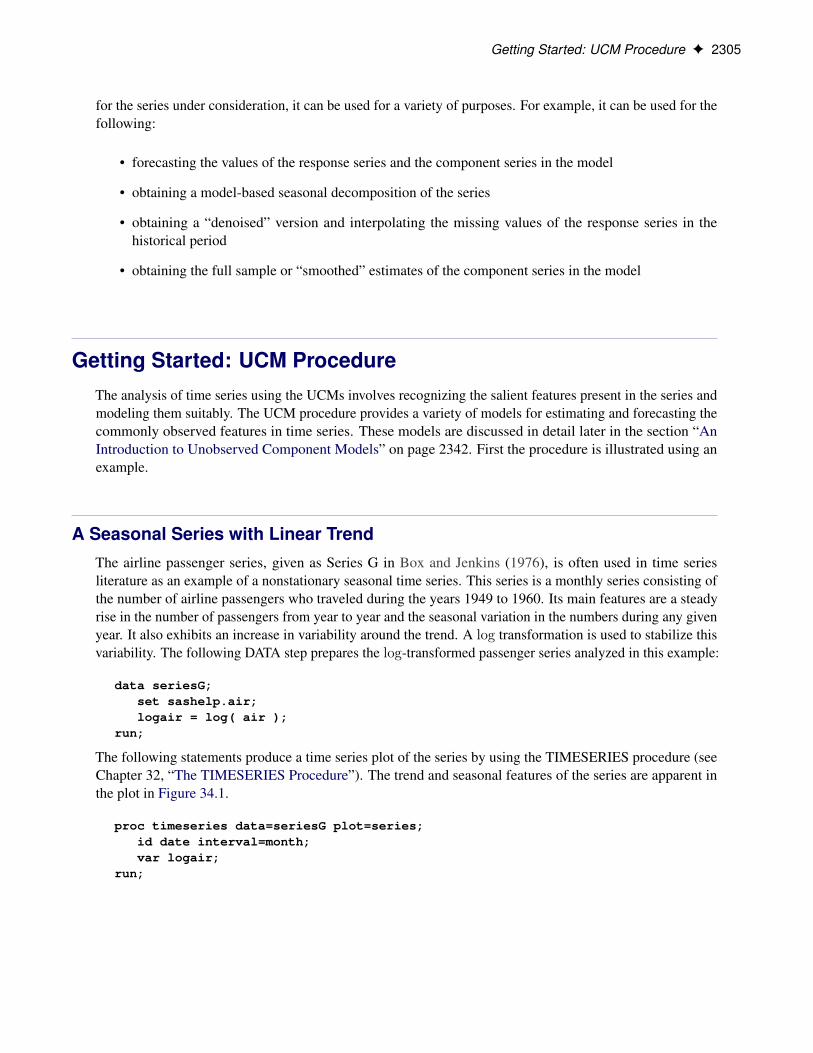
The following statements produce a time series plot of the series by using the TIMESERIES procedure (seeChapter 32, “The TIMESERIES Procedure”). The trend and seasonal features of the series are apparent inthe plot in Figure 34.1.
proc timeseries data=seriesG plot=series;id date interval=month;var logair;
run;

2306 F Chapter 34: The UCM Procedure
Figure 34.1 Series Plot of Log-Transformed Airline Passenger Series
In this example this series is modeled using an unobserved component model called the basic structuralmodel (BSM). The BSM models a time series as a sum of three stochastic components: a trend component�t , a seasonal component t , and random error �t . Formally, a BSM for a response series yt can be describedas
yt D �t C t C �t
Each of the stochastic components in the model is modeled separately. The random error �t , also calledthe irregular component, is modeled simply as a sequence of independent, identically distributed (i.i.d.)zero-mean Gaussian random variables. The trend and the seasonal components can be modeled in a fewdifferent ways. The model for trend used here is called a locally linear time trend. This trend model can bewritten as follows:
�t D �t�1 C ˇt�1 C �t ; �t � i:i:d: N.0; �2� /
ˇt D ˇt�1 C �t ; �t � i:i:d: N.0; �2� /
A Seasonal Series with Linear Trend F 2307
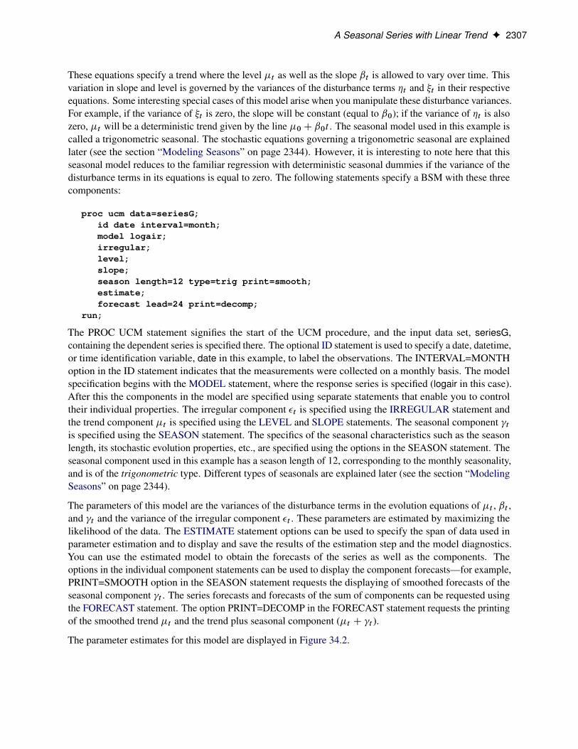
These equations specify a trend where the level �t as well as the slope ˇt is allowed to vary over time. Thisvariation in slope and level is governed by the variances of the disturbance terms �t and �t in their respectiveequations. Some interesting special cases of this model arise when you manipulate these disturbance variances.For example, if the variance of �t is zero, the slope will be constant (equal to ˇ0); if the variance of �t is alsozero, �t will be a deterministic trend given by the line �0C ˇ0t . The seasonal model used in this example iscalled a trigonometric seasonal. The stochastic equations governing a trigonometric seasonal are explainedlater (see the section “Modeling Seasons” on page 2344). However, it is interesting to note here that thisseasonal model reduces to the familiar regression with deterministic seasonal dummies if the variance of thedisturbance terms in its equations is equal to zero. The following statements specify a BSM with these threecomponents:
proc ucm data=seriesG;id date interval=month;model logair;irregular;level;slope;season length=12 type=trig print=smooth;estimate;forecast lead=24 print=decomp;
run;
The PROC UCM statement signifies the start of the UCM procedure, and the input data set, seriesG,containing the dependent series is specified there. The optional ID statement is used to specify a date, datetime,or time identification variable, date in this example, to label the observations. The INTERVAL=MONTHoption in the ID statement indicates that the measurements were collected on a monthly basis. The modelspecification begins with the MODEL statement, where the response series is specified (logair in this case).After this the components in the model are specified using separate statements that enable you to controltheir individual properties. The irregular component �t is specified using the IRREGULAR statement andthe trend component �t is specified using the LEVEL and SLOPE statements. The seasonal component tis specified using the SEASON statement. The specifics of the seasonal characteristics such as the seasonlength, its stochastic evolution properties, etc., are specified using the options in the SEASON statement. Theseasonal component used in this example has a season length of 12, corresponding to the monthly seasonality,and is of the trigonometric type. Different types of seasonals are explained later (see the section “ModelingSeasons” on page 2344).
The parameters of this model are the variances of the disturbance terms in the evolution equations of �t , ˇt ,and t and the variance of the irregular component �t . These parameters are estimated by maximizing thelikelihood of the data. The ESTIMATE statement options can be used to specify the span of data used inparameter estimation and to display and save the results of the estimation step and the model diagnostics.You can use the estimated model to obtain the forecasts of the series as well as the components. Theoptions in the individual component statements can be used to display the component forecasts—for example,PRINT=SMOOTH option in the SEASON statement requests the displaying of smoothed forecasts of theseasonal component t . The series forecasts and forecasts of the sum of components can be requested usingthe FORECAST statement. The option PRINT=DECOMP in the FORECAST statement requests the printingof the smoothed trend �t and the trend plus seasonal component (�t C t ).
The parameter estimates for this model are displayed in Figure 34.2.

2308 F Chapter 34: The UCM Procedure
Figure 34.2 BSM for the Logair Series
The UCM ProcedureThe UCM Procedure
Final Estimates of the Free Parameters
Component Parameter EstimateApprox
Std Error t ValueApproxPr > |t|
Irregular Error Variance 0.00023436 0.0001079 2.17 0.0298
Level Error Variance 0.00029828 0.0001057 2.82 0.0048
Slope Error Variance 8.47916E-13 6.2271E-10 0.00 0.9989
Season Error Variance 0.00000356 1.32347E-6 2.69 0.0072
The estimates suggest that except for the slope component, the disturbance variances of all the componentsare significant—that is, all these components are stochastic. The slope component, however, appears to bedeterministic because its error variance is quite insignificant. It might then be useful to check if the slopecomponent can be dropped from the model—that is, if ˇ0 D 0. This can be checked by examining thesignificance analysis table of the components given in Figure 34.3.
Figure 34.3 Component Significance Analysis for the Logair Series
Significance Analysis of Components(Based on the Final State)
Component DF Chi-Square Pr > ChiSq
Irregular 1 0.08 0.7747
Level 1 117867 <.0001
Slope 1 43.78 <.0001
Season 11 507.75 <.0001
This table provides the significance of the components in the model at the end of the estimation span. If acomponent is deterministic, this analysis is equivalent to checking whether the corresponding regressioneffect is significant. However, if a component is stochastic, then this analysis pertains only to the portion ofthe series near the end of the estimation span. In this example the slope appears quite significant and shouldbe retained in the model, possibly as a deterministic component. Note that, on the basis of this table, theirregular component’s contribution appears insignificant toward the end of the estimation span; however,since it is a stochastic component, it cannot be dropped from the model on the basis of this analysis alone.The slope component can be made deterministic by holding the value of its error variance fixed at zero. Thisis done by modifying the SLOPE statement as follows:
slope variance=0 noest;

A Seasonal Series with Linear Trend F 2309
After a tentative model is fit, its adequacy can be checked by examining different goodness-of-fit measuresand other diagnostic tests and plots that are based on the model residuals. Once the model appears satisfactory,it can be used for forecasting. An interesting feature of the UCM procedure is that, apart from the seriesforecasts, you can request the forecasts of the individual components in the model. The plots of componentforecasts can be useful in understanding their contributions to the series. The following statements illustratesome of these features:
proc ucm data=seriesG;id date interval = month;model logair;irregular;level plot=smooth;slope variance=0 noest;season length=12 type=trig
plot=smooth;estimate;forecast lead=24 plot=decomp;
run;
The table given in Figure 34.4 shows the goodness-of-fit statistics that are computed by using the one-step-ahead prediction errors (see the section “Statistics of Fit” on page 2380). These measures indicate a goodagreement between the model and the data. Additional diagnostic measures are also printed by default butare not shown here.
Figure 34.4 Fit Statistics for the Logair Series
The UCM ProcedureThe UCM Procedure
Fit Statistics Based on Residuals
Mean Squared Error 0.00147
Root Mean Squared Error 0.03830
Mean Absolute Percentage Error 0.54132
Maximum Percent Error 2.19097
R-Square 0.99061
Adjusted R-Square 0.99046
Random Walk R-Square 0.87288
Amemiya's Adjusted R-Square 0.99017
Number of non-missing residuals usedfor computing the fit statistics = 131
The first plot, shown in Figure 34.5, is produced by the PLOT=SMOOTH option in the LEVEL statement, itshows the smoothed level of the series.

2310 F Chapter 34: The UCM Procedure
Figure 34.5 Smoothed Trend in the Logair Series
The second plot (Figure 34.6), produced by the PLOT=SMOOTH option in the SEASON statement, showsthe smoothed seasonal component by itself.

A Seasonal Series with Linear Trend F 2311
Figure 34.6 Smoothed Seasonal in the Logair Series
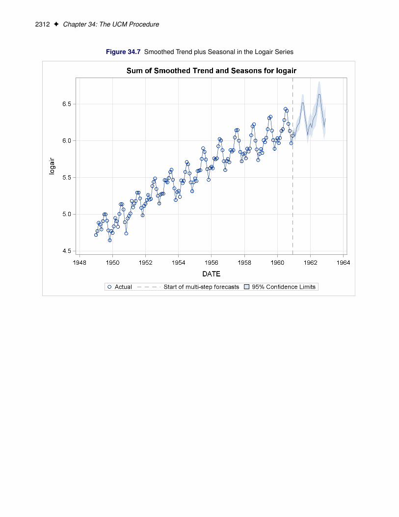
The plot of the sum of the trend and seasonal component, produced by the PLOT=DECOMP option in theFORECAST statement, is shown in Figure 34.7. You can see that, at least visually, the model seems to fit thedata well. In all these decomposition plots the component estimates are extrapolated for two years in thefuture based on the LEAD=24 option specified in the FORECAST statement.
2312 F Chapter 34: The UCM Procedure
Figure 34.7 Smoothed Trend plus Seasonal in the Logair Series
Syntax: UCM Procedure F 2313
Syntax: UCM ProcedureThe UCM procedure uses the following statements:
PROC UCM < options > ;AUTOREG < options > ;BLOCKSEASON options ;BY variables ;CYCLE < options > ;DEPLAG options ;ESTIMATE < options > ;FORECAST < options > ;ID variable options ;IRREGULAR < options > ;LEVEL < options > ;MODEL dependent variable < = regressors > ;NLOPTIONS options ;PERFORMANCE options ;OUTLIER options ;RANDOMREG regressors < / options > ;SEASON options ;SLOPE < options > ;SPLINEREG regressor < options > ;SPLINESEASON options ;
The PROC UCM and MODEL statements are required. In addition, the model must contain at least onecomponent with nonzero disturbance variance.
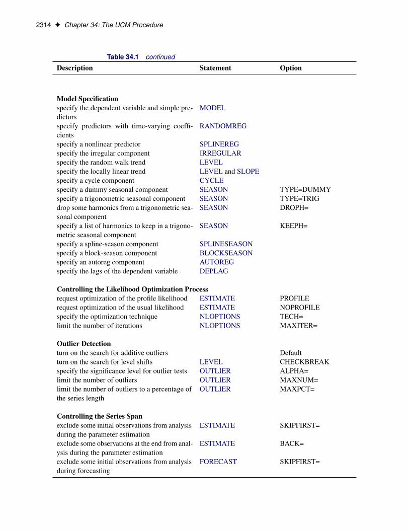
Functional SummaryThe statements and options controlling the UCM procedure are summarized in the following table. Mostcommonly needed scenarios are listed; see the individual statements for additional details. You can usethe PRINT= and PLOT= options in the individual component statements for printing and plotting thecorresponding component forecasts.
Table 34.1 Functional Summary
Description Statement Option
Data Set Optionsspecify the input data set PROC UCM DATA=write parameter estimates to an output data set ESTIMATE OUTEST=write series and component forecasts to an out-put data set
FORECAST OUTFOR=
2314 F Chapter 34: The UCM Procedure
Table 34.1 continued
Description Statement Option
Model Specificationspecify the dependent variable and simple pre-dictors
MODEL
specify predictors with time-varying coeffi-cients
RANDOMREG
specify a nonlinear predictor SPLINEREGspecify the irregular component IRREGULARspecify the random walk trend LEVELspecify the locally linear trend LEVEL and SLOPEspecify a cycle component CYCLEspecify a dummy seasonal component SEASON TYPE=DUMMYspecify a trigonometric seasonal component SEASON TYPE=TRIGdrop some harmonics from a trigonometric sea-sonal component
SEASON DROPH=
specify a list of harmonics to keep in a trigono-metric seasonal component
SEASON KEEPH=
specify a spline-season component SPLINESEASONspecify a block-season component BLOCKSEASONspecify an autoreg component AUTOREGspecify the lags of the dependent variable DEPLAG
Controlling the Likelihood Optimization Processrequest optimization of the profile likelihood ESTIMATE PROFILErequest optimization of the usual likelihood ESTIMATE NOPROFILEspecify the optimization technique NLOPTIONS TECH=limit the number of iterations NLOPTIONS MAXITER=
Outlier Detectionturn on the search for additive outliers Defaultturn on the search for level shifts LEVEL CHECKBREAKspecify the significance level for outlier tests OUTLIER ALPHA=limit the number of outliers OUTLIER MAXNUM=limit the number of outliers to a percentage ofthe series length
OUTLIER MAXPCT=
Controlling the Series Spanexclude some initial observations from analysisduring the parameter estimation
ESTIMATE SKIPFIRST=
exclude some observations at the end from anal-ysis during the parameter estimation
ESTIMATE BACK=
exclude some initial observations from analysisduring forecasting
FORECAST SKIPFIRST=
Functional Summary F 2315
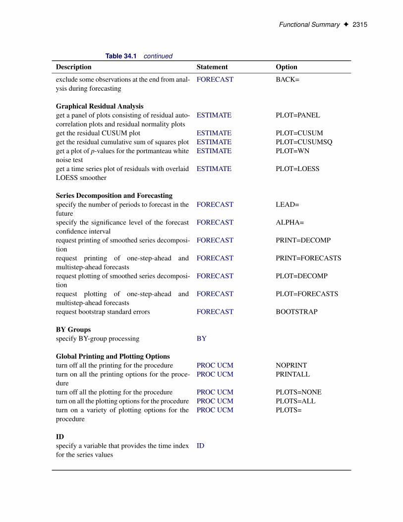
Table 34.1 continued
Description Statement Option
exclude some observations at the end from anal-ysis during forecasting
FORECAST BACK=
Graphical Residual Analysisget a panel of plots consisting of residual auto-correlation plots and residual normality plots
ESTIMATE PLOT=PANEL
get the residual CUSUM plot ESTIMATE PLOT=CUSUMget the residual cumulative sum of squares plot ESTIMATE PLOT=CUSUMSQget a plot of p-values for the portmanteau whitenoise test
ESTIMATE PLOT=WN
get a time series plot of residuals with overlaidLOESS smoother
ESTIMATE PLOT=LOESS
Series Decomposition and Forecastingspecify the number of periods to forecast in thefuture
FORECAST LEAD=
specify the significance level of the forecastconfidence interval
FORECAST ALPHA=
request printing of smoothed series decomposi-tion
FORECAST PRINT=DECOMP
request printing of one-step-ahead andmultistep-ahead forecasts
FORECAST PRINT=FORECASTS
request plotting of smoothed series decomposi-tion
FORECAST PLOT=DECOMP
request plotting of one-step-ahead andmultistep-ahead forecasts
FORECAST PLOT=FORECASTS
request bootstrap standard errors FORECAST BOOTSTRAP
BY Groupsspecify BY-group processing BY
Global Printing and Plotting Optionsturn off all the printing for the procedure PROC UCM NOPRINTturn on all the printing options for the proce-dure
PROC UCM PRINTALL
turn off all the plotting for the procedure PROC UCM PLOTS=NONEturn on all the plotting options for the procedure PROC UCM PLOTS=ALLturn on a variety of plotting options for theprocedure
PROC UCM PLOTS=
IDspecify a variable that provides the time indexfor the series values
ID

2316 F Chapter 34: The UCM Procedure
PROC UCM StatementPROC UCM < options > ;
The PROC UCM statement is required. The following options can be used in the PROC UCM statement:
DATA=SAS-data-setspecifies the name of the SAS data set containing the time series. If the DATA= option is not specifiedin the PROC UCM statement, the most recently created SAS data set is used.
NOPRINTturns off all the printing for the procedure. The subsequent print options in the procedure are ignored.
PLOTS< (global-plot-options) > < = plot-request < (options) > >
PLOTS< (global-plot-options) > < = (plot-request < (options) > < ... plot-request < (options) > >) >controls the plots produced with ODS Graphics. When you specify only one plot request, you can omitthe parentheses around the plot request.
Here are some examples:
plots=noneplots=allplots=residuals(acf loess)plots(noclm)=(smooth(decomp) residual(panel loess))
For general information about ODS Graphics, see Chapter 21, “Statistical Graphics Using ODS”(SAS/STAT User’s Guide).
proc ucm;model y = x;irregular;level;
run;
proc ucm plots=all;model y = x;irregular;level;
run;
The first PROC UCM step does not specify the PLOTS= option, so the default plot that displays theseries forecasts in the forecast region is produced. The PLOTS=ALL option in the second PROC UCMstep produces all the plots that are appropriate for the specified model.
In addition to the PLOTS= option in the PROC UCM statement, you can request plots by using thePLOT= option in other statements of the UCM procedure. This way of requesting plots provides finer

PROC UCM Statement F 2317
control over the plot production. If you do not specify any specific plot request, then PROC UCMproduces the plot of series forecasts in the forecast horizon by default.
Global Plot Options:The global-plot-options apply to all relevant plots generated by the UCM procedure. The followingglobal-plot-option is supported:
NOCLMsuppresses the confidence limits in all the component and forecast plots.
Specific Plot Options:The following list describes the specific plots and their options:
ALLproduces all plots appropriate for the particular analysis.
NONEsuppresses all plots.
FILTER (< filter-plot-options >)produces time series plots of the filtered component estimates. The following filter-plot-optionsare available:
ALLproduces all the filtered component estimate plots appropriate for the particular analysis.
LEVELproduces a time series plot of the filtered level component estimate, provided the modelcontains the level component.
SLOPEproduces a time series plot of the filtered slope component estimate, provided the modelcontains the slope component.
CYCLEproduces time series plots of the filtered cycle component estimates for all cycle componentsin the model, if there are any.
SEASONproduces time series plots of the filtered season component estimates for all seasonalcomponents in the model, if there are any.
DECOMPproduces time series plots of the filtered estimates of the series decomposition.
RESIDUAL ( < residual-plot-options >)produces the residuals plots. The following residual-plot-options are available:

2318 F Chapter 34: The UCM Procedure
ALLproduces all the residual diagnostics plots appropriate for the particular analysis.
ACFproduces the autocorrelation plot of residuals.
CUSUMproduces the plot of cumulative residuals against time.
CUSUMSQproduces the plot of cumulative squared residuals against time.
HISTOGRAMproduces the histogram of residuals.
LOESSproduces a scatter plot of residuals against time, which has an overlaid loess-fit.
PACFproduces the partial-autocorrelation plot of residuals.
PANELproduces a summary panel of the residual diagnostics consisting of the following:
• histogram of residuals
• normal quantile plot of residuals
• the residual-autocorrelation-plot
• the residual-partial-autocorrelation-plot
QQproduces a normal quantile plot of residuals.
RESIDUALproduces a needle plot of residuals against time.
WNproduces the plot of Ljung-Box white-noise test p-values at different lags (in log scale).
SMOOTH ( < smooth-plot-options >)produces time series plots of the smoothed component estimates. The following smooth-plot-options are available:
ALLproduces all the smoothed component estimate plots appropriate for the particular analysis.
LEVELproduces time series plot of the smoothed level component estimate, provided the modelcontains the level component.
AUTOREG Statement F 2319
SLOPEproduces time series plot of the smoothed slope component estimate, provided the modelcontains the slope component.
CYCLEproduces time series plots of the smoothed cycle component estimates for all cycle compo-nents in the model, if there are any.
SEASONproduces time series plots of the smoothed season component estimates for all seasoncomponents in the model, if there are any.
DECOMPproduces time series plots of the smoothed estimates of the series decomposition.
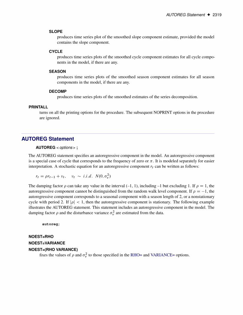
PRINTALLturns on all the printing options for the procedure. The subsequent NOPRINT options in the procedureare ignored.
AUTOREG StatementAUTOREG < options > ;
The AUTOREG statement specifies an autoregressive component in the model. An autoregressive componentis a special case of cycle that corresponds to the frequency of zero or � . It is modeled separately for easierinterpretation. A stochastic equation for an autoregressive component rt can be written as follows:
rt D �rt�1 C �t ; �t � i:i:d: N.0; �2� /
The damping factor � can take any value in the interval (–1, 1), including –1 but excluding 1. If � D 1, theautoregressive component cannot be distinguished from the random walk level component. If � D �1, theautoregressive component corresponds to a seasonal component with a season length of 2, or a nonstationarycycle with period 2. If j�j < 1, then the autoregressive component is stationary. The following exampleillustrates the AUTOREG statement. This statement includes an autoregressive component in the model. Thedamping factor � and the disturbance variance �2� are estimated from the data.
autoreg;
NOEST=RHO
NOEST=VARIANCE
NOEST=(RHO VARIANCE)fixes the values of � and �2� to those specified in the RHO= and VARIANCE= options.

2320 F Chapter 34: The UCM Procedure
PLOT=FILTERPLOT=SMOOTHPLOT=( < FILTER > < SMOOTH > )
requests plotting of the filtered or smoothed estimate of the autoreg component.
PRINT=FILTERPRINT=SMOOTHPRINT=(< FILTER > < SMOOTH >)
requests printing of the filtered or smoothed estimate of the autoreg component.
RHO=valuespecifies an initial value for the damping factor � during the parameter estimation process. The valueof � must be in the interval (–1, 1), including –1 but excluding 1.
VARIANCE=valuespecifies an initial value for the disturbance variance �2� during the parameter estimation process. Anynonnegative value, including zero, is an acceptable starting value.
BLOCKSEASON StatementBLOCKSEASON NBLOCKS = integer BLOCKSIZE = integer < options > ;
The BLOCKSEASON or BLOCKSEASONAL statement is used to specify a seasonal component t that hasa special block structure. The seasonal t is called a block seasonal of block size m and number of blocks kif its season length, s, can be factored as s D m � k and its seasonal effects have a block form—that is, thefirst m seasonal effects are all equal to some number �1, the next m effects are all equal to some number �2,and so on.
This type of seasonal structure can be appropriate in some cases; for example, consider a series that isrecorded on an hourly basis. Further assume that, in this particular case, the hour-of-the-day effect and theday-of-the-week effect are additive. In this situation the hour-of-the-week seasonality, having a season lengthof 168, can be modeled as a sum of two components. The hour-of-the-day effect is modeled using a simpleseasonal of season length 24, while the day-of-the-week is modeled as a block seasonal component that hasthe days of the week as blocks. This day-of-the-week block seasonal component has seven blocks, each ofsize 24.
A block seasonal specification requires, at the minimum, the block size m and the number of blocks in theseasonal k . These are specified using the BLOCKSIZE= and NBLOCKS= option, respectively. In addition,you might need to specify the position of the first observation of the series by using the OFFSET= option if itis not at the beginning of one of the blocks. In the example just considered, this corresponds to a situationwhere the first series measurement is not at the start of the day. Suppose that the first measurement of theseries corresponds to the hour between 6:00 and 7:00 a.m., which is the seventh hour within that day or at theseventh position within that block. This is specified as OFFSET=7.
The other options in this statement are very similar to the options in the SEASON statement; for example, ablock seasonal can also be of one of the two types, DUMMY and TRIG. There can be more than one blockseasonal component in the model, each specified using a separate BLOCKSEASON statement. No two block

BLOCKSEASON Statement F 2321
seasonals in the model can have the same NBLOCKS= and BLOCKSIZE= specifications. The followingexample illustrates the use of the BLOCKSEASON statement to specify the additive, hour-of-the-weekseasonal model:
season length=24 type=trig;blockseason nblocks=7 blocksize=24;
BLOCKSIZE=integerspecifies the block size, m. This is a required option in this statement. The block size can be anyinteger larger than or equal to two. Typical examples of block sizes are 24, corresponding to the hoursof the day when a day is being used as a block in hourly data, or 60, corresponding to the minutes inan hour when an hour is being used as a block in data recorded by minutes, etc.
NBLOCKS=integerspecifies the number of blocks, k . This is a required option in this statement. The number of blockscan be any integer greater than or equal to two.
NOESTfixes the value of the disturbance variance parameter to the value specified in the VARIANCE= option.
OFFSET=integerspecifies the position of the first measurement within the block, if the first measurement is not at thestart of a block. The OFFSET= value must be between one and the block size. The default value is one.The first measurement refers to the start of the estimation span and the forecast span. If these spansdiffer, their starting measurements must be separated by an integer multiple of the block size.
PLOT=FILTER
PLOT=SMOOTH
PLOT=F_ANNUAL
PLOT=S_ANNUAL
PLOT=( < plot request > . . . < plot request > )requests plots of the season component. When you specify only one plot request, you can omit theparentheses around the plot request. You can use the FILTER and SMOOTH options to plot the filteredand smoothed estimates of the season component t . You can use the F_ANNUAL and S_ANNUALoptions to get the plots of “annual” variation in the filtered and smoothed estimates of t . The annualplots are useful to see the change in the contribution of a particular month over the span of years. Here“month” and “year” are generic terms that change appropriately with the interval type being used tolabel the observations and the season length. For example, for monthly data with a season length of 12,the usual meaning applies, while for daily data with a season length of 7, the days of the week serve asmonths and the weeks serve as years. The first period in each block is plotted over the years.
PRINT=FILTER
PRINT=SMOOTH
PRINT=( < FILTER > < SMOOTH > )requests the printing of the filtered or smoothed estimate of the block seasonal component t .

2322 F Chapter 34: The UCM Procedure
TYPE=DUMMY | TRIGspecifies the type of the block seasonal component. The default type is DUMMY.
VARIANCE=valuespecifies an initial value for the disturbance variance, �2! , in the t equation at the start of the parameterestimation process. Any nonnegative value, including zero, is an acceptable starting value.
BY StatementBY variables ;
A BY statement can be used in the UCM procedure to process a data set in groups of observations defined bythe BY variables. The model specified using the MODEL and other component statements is applied to allthe groups defined by the BY variables. When a BY statement appears, the procedure expects the input dataset to be sorted in order of the BY variables. The variables are one or more variables in the input data set.
CYCLE StatementCYCLE < options > ;
The CYCLE statement is used to specify a cycle component, t , in the model. The stochastic equationgoverning a cycle component of period p and damping factor � is as follows�
t �t
�D �
�cos� sin�� sin� cos�
� � t�1 �t�1
�C
��t��t
�where �t and ��t are independent, zero-mean, Gaussian disturbances with variance �2� and � D 2 � �=p isthe angular frequency of the cycle. Any p strictly greater than two is an admissible value for the period, andthe damping factor � can be any value in the interval (0, 1), including one but excluding zero. The cycleswith frequency zero and � , which correspond to the periods equal to infinity and two, respectively, can bespecified using the AUTOREG statement. The values of � less than one give rise to a stationary cycle, while� D 1 gives rise to a nonstationary cycle. As a default, values of �, p, and �2� are estimated from the data.However, if necessary, you can fix the values of some or all of these parameters.
There can be multiple cycles in a model, each specified using a separate CYCLE statement. The examplesthat follow illustrate the use of the CYCLE statement.
The following statements request including two cycles in the model. The parameters of each of these cyclesare estimated from the data.
cycle;cycle;
The following statement requests inclusion of a nonstationary cycle in the model. The cycle period p and thedisturbance variance �2� are estimated from the data.
cycle rho=1 noest=rho;
DEPLAG Statement F 2323
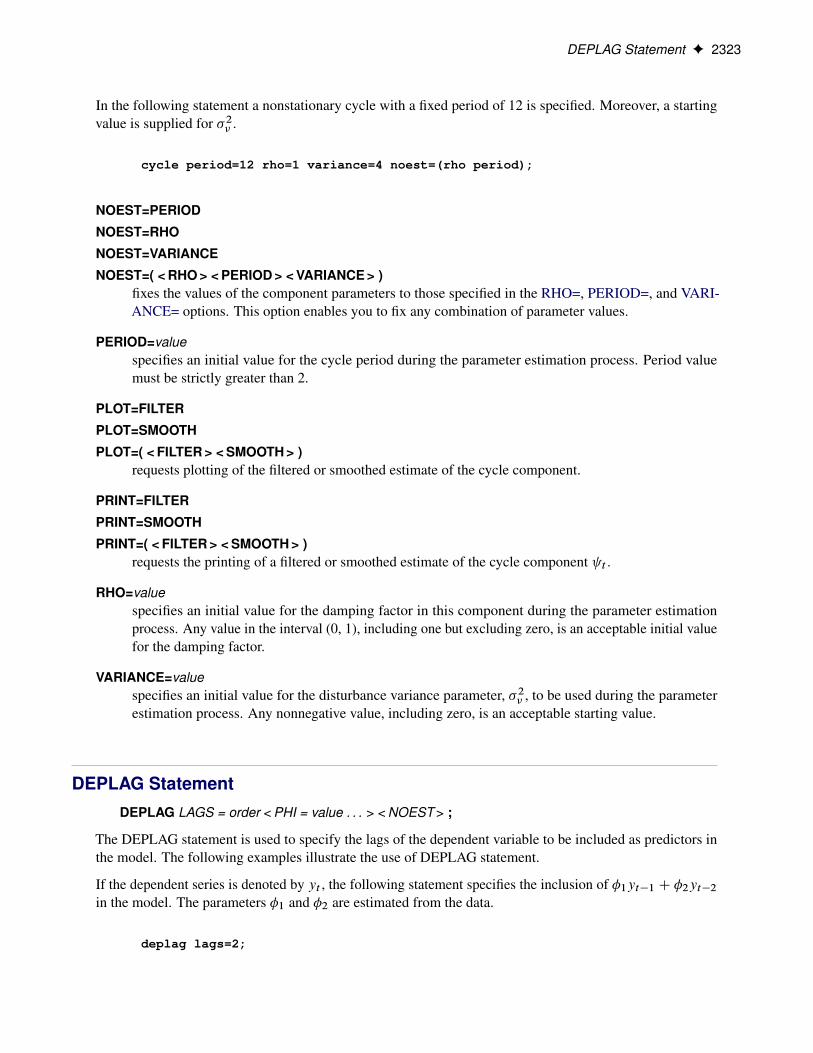
In the following statement a nonstationary cycle with a fixed period of 12 is specified. Moreover, a startingvalue is supplied for �2� .
cycle period=12 rho=1 variance=4 noest=(rho period);
NOEST=PERIOD
NOEST=RHO
NOEST=VARIANCE
NOEST=( < RHO > < PERIOD > < VARIANCE > )fixes the values of the component parameters to those specified in the RHO=, PERIOD=, and VARI-ANCE= options. This option enables you to fix any combination of parameter values.
PERIOD=valuespecifies an initial value for the cycle period during the parameter estimation process. Period valuemust be strictly greater than 2.
PLOT=FILTER
PLOT=SMOOTH
PLOT=( < FILTER > < SMOOTH > )requests plotting of the filtered or smoothed estimate of the cycle component.
PRINT=FILTER
PRINT=SMOOTH
PRINT=( < FILTER > < SMOOTH > )requests the printing of a filtered or smoothed estimate of the cycle component t .
RHO=valuespecifies an initial value for the damping factor in this component during the parameter estimationprocess. Any value in the interval (0, 1), including one but excluding zero, is an acceptable initial valuefor the damping factor.
VARIANCE=valuespecifies an initial value for the disturbance variance parameter, �2� , to be used during the parameterestimation process. Any nonnegative value, including zero, is an acceptable starting value.
DEPLAG StatementDEPLAG LAGS = order < PHI = value . . . > < NOEST > ;
The DEPLAG statement is used to specify the lags of the dependent variable to be included as predictors inthe model. The following examples illustrate the use of DEPLAG statement.
If the dependent series is denoted by yt , the following statement specifies the inclusion of �1yt�1 C �2yt�2in the model. The parameters �1 and �2 are estimated from the data.
deplag lags=2;
2324 F Chapter 34: The UCM Procedure
The following statement requests including �1yt�1 C �2yt�4 � �1�2yt�5 in the model. The values of �1and �2 are fixed at 0.8 and –1.2.
deplag lags=(1)(4) phi=0.8 -1.2 noest;
The dependent lag parameters are not constrained to lie in any particular region. In particular, this implies thata UCM that contains only an irregular component and dependent lags, resulting in a traditional autoregressivemodel, is not constrained to be a stationary model. In the DEPLAG statement, if an initial value is suppliedfor any one of the parameters, the initial values must also be supplied for all other parameters.
LAGS=order
LAGS=(lag, . . . , lag ) . . . (lag, . . . , lag )is a required option in this statement. LAGS=(l 1, l 2, . . . , l k ) defines a model with specified lags ofthe dependent variable included as predictors. LAGS=order is equivalent to LAGS=(1, 2, . . . , order ).
A concatenation of parenthesized lists specifies a factored model. For example, LAGS=(1)(12) specifiesthat the lag values, 1, 12, and 13, corresponding to the following polynomial in the backward shiftoperator, be included in the model
.1 � �1;1B/.1 � �2;1B12/
Note that, in this case, the coefficient of the thirteenth lag is constrained to be the product of thecoefficients of the first and twelfth lags.
NOESTfixes the values of the parameters to those specified in PHI= option.
PHI=value . . .lists starting values for the coefficients of the lagged dependent variable. The order of the values listedcorresponds with the order of the lags specified in the LAGS= option.
ESTIMATE StatementESTIMATE < options > ;
The ESTIMATE statement is an optional statement used to control the overall model-fitting environment.Using this statement, you can control the span of observations used to fit the model by using the SKIPFIRST=and BACK= options. This can be useful in model diagnostics. You can request a variety of goodness-of-fitstatistics and other model diagnostic information including different residual diagnostic plots. Note that theESTIMATE statement is not used to control the nonlinear optimization process itself. That is done usingthe NLOPTIONS statement, where you can control the number of iterations, choose between the differentoptimization techniques, and so on. You can save the estimated parameters and other related informationin a data set by using the OUTEST= option. You can request the optimization of the profile likelihood,the likelihood obtained by concentrating out a disturbance variance, for parameter estimation by using thePROFILE option. The following example illustrates the use of this statement:
estimate skipfirst=12 back=24;

ESTIMATE Statement F 2325
This statement requests that the initial 12 measurements and the last 24 measurements be excluded during themodel-fitting process. The actual observation span used to fit the model is decided as follows: Suppose thatn0 and n1 are the observation numbers of the first and the last nonmissing values of the response variable,respectively. As a result of SKIPFIRST=12 and BACK=24, the measurements between observation numbersn0 C 12 and n1 � 24 form the estimation span. Of course, the model fitting might not take place if thereare insufficient data in the resulting span. The model fitting does not take place if there are regressors in themodel that have missing values in the estimation span.
BACK=integer
SKIPLAST=integerindicates that some ending part of the data needs to be ignored during the parameter estimation. Thiscan be useful when you want to study the forecasting performance of a model on the observed data.BACK=10 results in skipping the last 10 measurements of the response series during the parameterestimation. The default is BACK=0.
EXTRADIFFUSE=kenables continuation of the diffuse filtering iterations for k additional iterations beyond the first instancewhere the initialization of the diffuse state would have otherwise taken place. If the specified k is largerthan the sample size, the diffuse iterations continue until the end of the sample. Note that one-step-ahead residuals are produced only after the diffuse state is initialized. Delaying the initialization leadsto a reduction in the number of one-step-ahead residuals available for computing the residual diagnosticmeasures. This option is useful when you want to ignore the first few one-step-ahead residuals thatoften have large variance.
NOPROFILErequests that the usual likelihood be optimized for parameter estimation. For more information, see thesection “Parameter Estimation by Profile Likelihood Optimization” on page 2358.
OUTEST=SAS-data-setspecifies an output data set for the estimated parameters.
In the ESTIMATE statement, the PLOT= option is used to obtain different residual diagnostic plots.The different possibilities are as follows:
PLOT=ACF
PLOT=MODEL
PLOT=LOESS
PLOT=HISTOGRAM
PLOT=PACF
PLOT=PANEL
PLOT=QQ
PLOT=RESIDUAL
PLOT=WN
PLOT=( < plot request > . . . < plot request > )requests different residual diagnostic plots. The different options are as follows:

2326 F Chapter 34: The UCM Procedure
ACFproduces the residual-autocorrelation plot.
CUSUMproduces the plot of cumulative residuals against time.
CUSUMSQproduces the plot of cumulative squared residuals against time.
MODELproduces the plot of one-step-ahead forecasts in the estimation span.
HISTOGRAMproduces the histogram of residuals.
LOESSproduces a scatter plot of residuals against time, which has an overlaid loess-fit.
PACFproduces the residual-partial-autocorrelation plot.
PANELproduces a summary panel of the residual diagnostics consisting of
• histogram of residuals• normal quantile plot of residuals• the residual-autocorrelation-plot• the residual-partial-autocorrelation-plot
QQproduces a normal quantile plot of residuals.
RESIDUALproduces a needle plot of residuals against time.
WNproduces a plot of p-values, in log-scale, at different lags for the Ljung-Box portmanteau whitenoise test statistics.
PRINT=NONEsuppresses all the printed output related to the model fitting, such as the parameter estimates, thegoodness-of-fit statistics, and so on.
PROFILErequests that the profile likelihood, obtained by concentrating out one of the disturbance variancesfrom the likelihood, be optimized for parameter estimation. By default, the profile likelihood is notoptimized if any of the disturbance variance parameters is held fixed to a nonzero value. For moreinformation see the section “Parameter Estimation by Profile Likelihood Optimization” on page 2358.

FORECAST Statement F 2327
SKIPFIRST=integerindicates that some early part of the data needs to be ignored during the parameter estimation. Thiscan be useful if there is a reason to believe that the model being estimated is not appropriate for thisportion of the data. SKIPFIRST=10 results in skipping the first 10 measurements of the response seriesduring the parameter estimation. The default is SKIPFIRST=0.
FORECAST StatementFORECAST < options > ;
The FORECAST statement is an optional statement that is used to specify the overall forecasting environmentfor the specified model. It can be used to specify the span of observations, the historical period, to use tocompute the forecasts of the future observations. This is done using the SKIPFIRST= and BACK= options.The number of periods to forecast beyond the historical period, and the significance level of the forecastconfidence interval, is specified using the LEAD= and ALPHA= options. You can request one-step-aheadseries and component forecasts by using the PRINT= option. You can save the series forecasts, and themodel-based decomposition of the series, in a data set by using the OUTFOR= option. You can use theBOOTSTRAP option to request the computation of bootstrap prediction standard errors and the associatedconfidence intervals. The following example illustrates the use of this statement:
forecast skipfirst=12 back=24 lead=30;
This statement requests that the initial 12 and the last 24 response values be excluded during the forecastcomputations. The forecast horizon, specified using the LEAD= option, is 30 periods; that is, multistepforecasting begins at the end of the historical period and continues for 30 periods. The actual observation spanused to compute the multistep forecasting is decided as follows: Suppose that n0 and n1 are the observationnumbers of the first and the last nonmissing values of the response variable, respectively. As a result ofSKIPFIRST=12 and BACK=24, the historical period, or the forecast span, begins at n0 C 12 and ends atn1 � 24. Multistep forecasts are produced for the next 30 periods—that is, for the observation numbersn1� 23 to n1C 6. Of course, the forecast computations can fail if the model has regressor variables that havemissing values in the forecast span. If the regressors contain missing values in the forecast horizon—that is,between the observations n1 � 23 and n1 C 6—the forecast horizon is reduced accordingly.
ALPHA=valuespecifies the significance level of the forecast confidence intervals; for example, ALPHA=0.05, whichis the default, results in a 95% confidence interval.
BACK=integer
SKIPLAST=integerspecifies the holdout sample for the evaluation of the forecasting performance of the model. Forexample, BACK=10 results in treating the last 10 observed values of the response series as unobserved.A post-sample-prediction-analysis table is produced for comparing the predicted values with the actualvalues in the holdout period. The default is BACK=0.
BOOTSTRAP(NREP=integer < SEED=integer >) (Experimental )enables the computation of bootstrap prediction standard errors based on the specified number ofreplications (NREP). The value of NREP must be at least 2. Optionally, you can specify the random

2328 F Chapter 34: The UCM Procedure
number seed that is associated with the first replication by using the SEED= option. The seeds for thesubsequent replications are assigned sequentially. The default seed value that is associated with the firstreplication is 123. The BOOTSTRAP option has no effect if the number of parameters to be estimatedis zero (that is, all the model parameters are known). Note that this option is computationally expensive.The computational cost of NREP replications is comparable to the cost of estimating parameters NREPtimes.
EXTRADIFFUSE=kenables continuation of the diffuse filtering iterations for k additional iterations beyond the first instancewhere the initialization of the diffuse state would have otherwise taken place. If the specified k is largerthan the sample size, the diffuse iterations continue until the end of the sample. Note that one-step-ahead forecasts are produced only after the diffuse state is initialized. Delaying the initialization leadsto reduction in the number of one-step-ahead forecasts. This option is useful when you want to ignorethe first few one-step-ahead forecasts that often have large variance.
LEAD=integerspecifies the number of periods to forecast beyond the historical period defined by the SKIPFIRST=and BACK= options; for example, LEAD=10 results in the forecasting of 10 future values of theresponse series. The default is LEAD=12.
OUTFOR=SAS-data-setspecifies an output data set for the forecasts. The output data set contains the ID variable (if specified),the response and predictor series, the one-step-ahead and out-of-sample response series forecasts, theforecast confidence intervals, the smoothed values of the response series, and the smoothed forecastsproduced as a result of the model-based decomposition of the series.
PLOT=DECOMP
PLOT=DECOMPVAR
PLOT=FDECOMP
PLOT=FDECOMPVAR
PLOT=FORECASTS
PLOT=TREND
PLOT=( < plot request > . . . < plot request > )requests forecast and model decomposition plots. The FORECASTS option provides the plot of theseries forecasts, the TREND and DECOMP options provide the plots of the smoothed trend and otherdecompositions, the DECOMPVAR option can be used to plot the variance of these components, andthe FDECOMP and FDECOMPVAR options provide the same plots for the filtered decompositionestimates and their variances.
PRINT=DECOMP
PRINT=FDECOMP
PRINT=FORECASTS
PRINT=NONE
PRINT=( < print request > . . . < print request > )controls the printing of the series forecasts and the printing of smoothed model decomposition estimates.By default, the series forecasts are printed only for the forecast horizon specified by the LEAD= option;that is, the one-step-ahead predicted values are not printed. You can request forecasts for the entire

ID Statement F 2329
forecast span by specifying the PRINT=FORECASTS option. Using PRINT=DECOMP, you canget smoothed estimates of the following effects: trend, trend plus regression, trend plus regressionplus cycle, and sum of all components except the irregular. If some of these effects are absent inthe model, then they are ignored. Similarly you can get filtered estimates of these effects by usingPRINT=FDECOMP. You can use PRINT=NONE to suppress the printing of all the forecast output.
SKIPFIRST=integerindicates that some early part of the data needs to be ignored during the forecasting calculations. Thiscan be useful if there is a reason to believe that the model being used for forecasting is not appropriatefor this portion of the data. SKIPFIRST=10 results in skipping the first 10 measurements of theresponse series during the forecast calculations. The default is SKIPFIRST=0.
ID StatementID variable INTERVAL=value < ALIGN=value > ;
The ID statement names a numeric variable that identifies observations in the input and output data sets. TheID variable’s values are assumed to be SAS date, time, or datetime values. In addition, the ID statementspecifies the frequency associated with the time series. The ID statement options also specify how theobservations are aligned to form the time series. If the ID statement is specified, the INTERVAL= optionmust also be specified. If the ID statement is not specified, the observation number, with respect to the BYgroup, is used as the time ID. The values of the ID variable are extrapolated for the forecast observationsbased on the values of the INTERVAL= option.
ALIGN=valuecontrols the alignment of SAS dates used to identify output observations. The ALIGN= option has thefollowing possible values: BEGINNING | BEG | B, MIDDLE | MID | M, and ENDING | END | E.The default is BEGINNING. The ALIGN= option is used to align the ID variable with the beginning,middle, or end of the time ID interval specified by the INTERVAL= option.
INTERVAL=valuespecifies the time interval between observations. This option is required in the ID statement. INTER-VAL=value is used in conjunction with the ID variable to check that the input data are in order andhave no gaps. The INTERVAL= option is also used to extrapolate the ID values past the end of theinput data. For a complete discussion of the intervals supported, please see Chapter 4, “Date Intervals,Formats, and Functions.”
IRREGULAR StatementIRREGULAR < options > ;
The IRREGULAR statement includes an irregular component in the model. There can be at most oneIRREGULAR statement in the model specification. The irregular component corresponds to the overallrandom error �t in the model. By default the irregular component is modeled as white noise—that is, as asequence of independent, identically distributed, zero-mean, Gaussian random variables. However, you canalso model it as an autoregressive moving average (ARMA) process. The options for specifying an ARMAmodel for the irregular component are given in a separate subsection: “ARMA Specification” on page 2330.
2330 F Chapter 34: The UCM Procedure
The options in this statement enable you to specify the model for the irregular component and to output itsestimates. Two examples of the IRREGULAR statement are given next. In the first example the statement isin its simplest form, resulting in the inclusion of an irregular component that is white noise with unknownvariance:
irregular;
The following statement provides a starting value for the white noise variance �2� to be used in the nonlinearparameter estimation process. It also requests the printing of smoothed estimates of �t . The smoothedirregulars are useful in model diagnostics.
irregular variance=4 print=smooth;
NOESTfixes the value of �2� to the value specified in the VARIANCE= option. Also see the NOEST= optionin the subsection “ARMA Specification” on page 2330.
PLOT=FILTER
PLOT=SMOOTH
PLOT=( < FILTER > < SMOOTH > )requests plotting of the filtered or smoothed estimate of the irregular component.
PRINT=FILTER
PRINT=SMOOTH
PRINT=( < FILTER > < SMOOTH > )requests printing of the filtered or smoothed estimate of the irregular component.
VARIANCE=valuespecifies an initial value for �2� during the parameter estimation process. Any nonnegative value,including zero, is an acceptable starting value.
ARMA Specification
This section details the options for specifying an ARMA model for the irregular component. The specificationof ARMA models requires some notation, which is explained first.
Let B denote the backshift operator—that is, for any sequence �t , B�t D �t�1. The higher powersof B represent larger shifts (for example, B3�t D �t�3). A random sequence �t follows a zero-meanARMA(p,q)�(P,Q)s model with nonseasonal autoregressive order p, seasonal autoregressive order P, nonsea-sonal moving average order q, and seasonal moving average order Q, if it satisfies the following differenceequation specified in terms of the polynomials in the backshift operator where at is a white noise sequenceand s is the season length:
�.B/ˆ.Bs/�t D �.B/‚.Bs/at
The polynomials �;ˆ; �; and ‚ are of orders p, P, q, and Q, respectively, which can be any nonnegativeintegers. The season length s must be a positive integer. For example, �t satisfies an ARMA(1,1) model (thatis, p D 1; q D 1; P D 0; and Q D 0) if
�t D �1�t�1 C at � �1at�1
IRREGULAR Statement F 2331
for some coefficients �1 and �1 and a white noise sequence at . Similarly �t satisfies an ARMA(1,1)�(1,1)12model if
�t D �1�t�1 Cˆ1�t�12 � �1ˆ1�t�13 C at � �1at�1 �‚1at�12 C �1‚1at�13
for some coefficients �1; ˆ1; �1; and ‚1 and a white noise sequence at . The ARMA process is stationaryand invertible if the defining polynomials �;ˆ; �; and ‚ have all their roots outside the unit circle—thatis, their absolute values are strictly larger than 1.0. It is assumed that the ARMA model specified for theirregular component is stationary and invertible—that is, the coefficients of the polynomials �;ˆ; �; and ‚are constrained so that the stationarity and invertibility conditions are satisfied. The unknown coefficients ofthese polynomials become part of the model parameter vector that is estimated using the data.
The notation for a closely related class of models, autoregressive integrated moving average (ARIMA)models, is also given here. A random sequence yt is said to follow an ARIMA(p,d,q)�(P,D,Q)s modelif, for some nonnegative integers d and D, the differenced series �t D .1 � B/d .1 � Bs/Dyt follows anARMA(p,q)�(P,Q)s model. The integers d and D are called nonseasonal and seasonal differencing orders,respectively. You can specify ARIMA models by using the DEPLAG statement for specifying the differencingorders and by using the IRREGULAR statement for the ARMA specification. See Example 34.8 for anexample of ARIMA(0,1,1)�(0,1,1)12 model specification. Brockwell and Davis (1991) can be consulted foradditional information about ARIMA models.
You can use options of the IRREGULAR statement to specify the desired ARMA model and to requestprinted and graphical output. A few examples of the IRREGULAR statement are given next.
The following statement specifies an irregular component that is modeled as an ARMA(1,1) process. It alsorequests plotting its smoothed estimate.
irregular p=1 q=1 plot=smooth;
The following statement specifies an ARMA(1,1)�(1,1)12 model. It also fixes the coefficient of the first-orderseasonal moving average polynomial to 0.1. The other coefficients and the white noise variance are estimatedusing the data.
irregular p=1 sp=1 q=1 sq=1 s=12 sma=0.1 noest=(sma);
AR=�1 �2 . . .�plists the starting values of the coefficients of the nonseasonal autoregressive polynomial
�.B/ D 1 � �1B � : : : � �pBp
where the order p is specified in the P= option. The coefficients �i must define a stationary autoregres-sive polynomial.
MA=�1 �2 . . . �qlists the starting values of the coefficients of the nonseasonal moving average polynomial
�.B/ D 1 � �1B � : : : � �qBq
where the order q is specified in the Q= option. The coefficients �i must define an invertible movingaverage polynomial.

2332 F Chapter 34: The UCM Procedure
NOEST=(<VARIANCE> <AR> <SAR> <MA> <SMA>)fixes the values of the ARMA parameters and the value of the white noise variance to those specifiedin the AR=, SAR=, MA=, SMA=, or VARIANCE= options.
P=integerspecifies the order of the nonseasonal autoregressive polynomial. The order can be any nonnegativeinteger; the default value is 0. In practice the order is a small integer such as 1, 2, or 3.
Q=integerspecifies the order of the nonseasonal moving average polynomial. The order can be any nonnegativeinteger; the default value is 0. In practice the order is a small integer such as 1, 2, or 3.
S=integerspecifies the season length used during the specification of the seasonal autoregressive or seasonalmoving average polynomial. The season length can be any positive integer; for example, S=4 might bean appropriate value for a quarterly series. The default value is S=1.
SAR=ˆ1 ˆ2 . . .ˆPlists the starting values of the coefficients of the seasonal autoregressive polynomial
ˆ.Bs/ D 1 �ˆ1Bs� : : : �ˆPB
sP
where the order P is specified in the SP= option and the season length s is specified in the S= option.The coefficients ˆi must define a stationary autoregressive polynomial.
SMA=‚1 ‚2 . . .‚Qlists the starting values of the coefficients of the seasonal moving average polynomial
‚.Bs/ D 1 �‚1Bs� : : : �‚QB
sQ
where the order Q is specified in the SQ= option and the season length s is specified in the S= option.The coefficients ‚i must define an invertible moving average polynomial.
SP=integerspecifies the order of the seasonal autoregressive polynomial. The order can be any nonnegative integer;the default value is 0. In practice the order is a small integer such as 1 or 2.
SQ=integerspecifies the order of the seasonal moving average polynomial. The order can be any nonnegativeinteger; the default value is 0. In practice the order is a small integer such as 1 or 2.
LEVEL StatementLEVEL < options > ;
The LEVEL statement is used to include a level component in the model. The level component, either byitself or together with a slope component (see the SLOPE statement), forms the trend component, �t , ofthe model. If the slope component is absent, the resulting trend is a random walk (RW) specified by thefollowing equations:
�t D �t�1 C �t ; �t � i:i:d: N.0; �2� /

LEVEL Statement F 2333
If the slope component is present, signified by the presence of a SLOPE statement, a locally linear trend(LLT) is obtained. The equations of LLT are as follows:
�t D �t�1 C ˇt�1 C �t ; �t � i:i:d: N.0; �2� /
ˇt D ˇt�1 C �t ; �t � i:i:d: N.0; �2� /
In either case, the options in the LEVEL statement are used to specify the value of �2� and to request forecastsof �t . The SLOPE statement is used for similar purposes in the case of slope ˇt . The following examplesillustrate the use of the LEVEL statement. Assuming that a SLOPE statement is not added subsequently, asimple random walk trend is specified by the following statement:
level;
The following statements specify a locally linear trend with value of �2� fixed at 4. It also requests printing offiltered values of �t . The value of �2
�, the disturbance variance in the slope equation, is estimated from the
data.
level variance=4 noest print=filter;slope;
CHECKBREAKturns on the checking of breaks in the level component.
NOESTfixes the value of �2� to the value specified in the VARIANCE= option.
PLOT=FILTER
PLOT=SMOOTH
PLOT=( < FILTER > < SMOOTH > )requests plotting of the filtered or smoothed estimate of the level component.
PRINT=FILTER
PRINT=SMOOTH
PRINT=( < FILTER > < SMOOTH > )requests printing of the filtered or smoothed estimate of the level component.
VARIANCE=valuespecifies an initial value for �2� , the disturbance variance in the �t equation at the start of the parameterestimation process. Any nonnegative value, including zero, is an acceptable starting value.

2334 F Chapter 34: The UCM Procedure
MODEL StatementMODEL dependent < = regressors > ;
The MODEL statement specifies the response variable and, optionally, the predictor or regressor variables forthe UCM model. This is a required statement in the UCM procedure. The predictors specified in the MODELstatement are assumed to have a linear and time-invariant relationship with the response. The predictors thathave time-varying regression coefficients are specified separately in the RANDOMREG statement. Similarly,the predictors that have a nonlinear effect on the response variable are specified separately in the SPLINEREGstatement. Only one MODEL statement can be specified.
NLOPTIONS StatementNLOPTIONS < options > ;
PROC UCM uses the nonlinear optimization (NLO) subsystem to perform the nonlinear optimization of thelikelihood function during the estimation of model parameters. You can use the NLOPTIONS statementto control different aspects of this optimization process. For most problems the default settings of theoptimization process are adequate. However, in some cases it might be useful to change the optimizationtechnique or to change the maximum number of iterations. This can be done by using the TECH= andMAXITER= options in the NLOPTIONS statement as follows:
nloptions tech=dbldog maxiter=200;
This sets the maximum number of iterations to 200 and changes the optimization technique to DBLDOGrather than the default technique, TRUREG, used in PROC UCM. A discussion of the full range of optionsthat can be used with the NLOPTIONS statement is given in Chapter 6, “Nonlinear Optimization Methods.”In PROC UCM all these options are available except the options related to the printing of the optimizationhistory. In this version of PROC UCM all the printed output from the NLO subsystem is suppressed.
OUTLIER StatementOUTLIER < options > ;
The OUTLIER statement enables you to control the reporting of the additive outliers (AO) and level shifts(LS) in the response series. The AOs are searched by default. You can turn on the search for LSs by using theCHECKBREAK option in the LEVEL statement.
ALPHA=significance-levelspecifies the significance level for reporting the outliers. The default is 0.05.
MAXNUM=numberlimits the number of outliers to search. The default is MAXNUM=5.

PERFORMANCE Statement F 2335
MAXPCT=numberis similar to the MAXNUM= option. In the MAXPCT= option you can limit the number of outliers tosearch for according to a percentage of the series length. The default is MAXPCT=1. When both ofthese options are specified, the minimum of the two search numbers is used.
PRINT=SHORT | DETAILenables you to control the printed output of the outlier search. The PRINT=SHORT option, whichis the default, produces an outlier summary table containing the most significant outliers, either AOor LS, discovered in the outlier search. The PRINT=DETAIL option produces, in addition to theoutlier summary table, separate tables containing the AO and LS structural break chi-square statisticscomputed at each time point in the estimation span.
PERFORMANCE StatementPERFORMANCE options ;
The PERFORMANCE statement defines performance parameters for distributed and multithreaded computingand passes variables that describe the distributed computing environment. In the UCM procedure, thisstatement is applicable only if you specify the BOOTSTRAP option in the FORECAST statement. Inaddition, the number of nodes that you specify in the NODES= option in the PERFORMANCE statementmust be strictly smaller than the number of bootstrap replications that you specify in the BOOTSTRAPoption. The following statements illustrate how you can use this statement to perform bootstrap computationsthat use 10 nodes on a grid named hpa.sas.com:
proc ucm data=seriesG;id date interval=month;model logair;irregular;level;forecast lead=24 bootstrap(nrep=50 seed=1234);performance nodes=10 host="hpa.sas.com";
run;
For more information about the PERFORMANCE statement, see the section “PERFORMANCE Statement”(Chapter 3, SAS/ETS User’s Guide: High-Performance Procedures).
RANDOMREG StatementRANDOMREG regressors < / options > ;
The RANDOMREG statement is used to specify regressors with time-varying regression coefficients. Eachregression coefficient—say, ˇt— is assumed to evolve as a random walk:
ˇt D ˇt�1 C �t ; �t � i:i:d: N.0; �2/
Of course, if the random walk disturbance variance �2 is zero, then the regression coefficient is not timevarying, and it reduces to the standard regression setting. There can be multiple RANDOMREG statements,and each statement can contain one or more regressors. The regressors in a given RANDOMREG statementform a group that is assumed to share the same disturbance variance parameter. The random walks associated

2336 F Chapter 34: The UCM Procedure
with different regressors are assumed to be independent. For an example of using this statement seeExample 34.4. See the section “Reporting Parameter Estimates for Random Regressors” on page 2354 foradditional information about the way parameter estimates are reported for this type of regressors.
NOESTfixes the value of �2 to the value specified in the VARIANCE= option.
PLOT=FILTER
PLOT=SMOOTH
PLOT=( < FILTER > < SMOOTH > )requests plotting of filtered or smoothed estimate of the time-varying regression coefficient.
PRINT=FILTER
PRINT=SMOOTH
PRINT=( < FILTER > < SMOOTH > )requests printing of the filtered or smoothed estimate of the time-varying regression coefficient.
VARIANCE=valuespecifies an initial value for �2 during the parameter estimation process. Any nonnegative value,including zero, is an acceptable starting value.
SEASON StatementSEASON LENGTH = integer < options > ;
The SEASON or SEASONAL statement is used to specify a seasonal component, t , in the model. Aseasonal component can be one of the two types, DUMMY or TRIG. A DUMMY seasonal with seasonlength s satisfies the following stochastic equation:
s�1XiD0
t�i D !t ; !t � i:i:d: N.0; �2!/
The equations for a TRIG (short for trigonometric) seasonal component are as follows
t D
Œs=2�XjD1
j;t
where Œs=2� equals s=2 if s is even and .s � 1/=2 if it is odd. The sinusoids, also called harmonics, j;t havefrequencies �j D 2�j=s and are specified by the matrix equation�
j;t �j;t
�D
�cos�j sin�j� sin�j cos�j
� � j;t�1 �j;t�1
�C
�!j;t!�j;t
�where the disturbances !j;t and !�j;t are assumed to be independent and, for fixed j, !j;t and !�j;t � N.0; �
2!/.
If s is even, then the equation for �s=2;t
is not needed and s=2;t is given by
s=2;t D � s=2;t�1 C !s=2;t

SEASON Statement F 2337
In the TRIG seasonal case, the option KEEPH= or DROPH= can be used to obtain subset trigonometricseasonals that contain only a subset of the full set of harmonics j;t , j D 1; 2; : : : ; Œs=2�. This is particularlyuseful when the season length s is large and the seasonal pattern is relatively smooth.
Note that whether the seasonal type is DUMMY or TRIG, there is only one parameter, the disturbancevariance �2! , in the seasonal model.
There can be more than one seasonal component in the model, necessarily with different season lengths if theseasons are full. You can have multiple subset season components with the same season length, if you needto use separate disturbance variances for different sets of harmonics. Each seasonal component is specifiedusing a separate SEASON statement. A model with multiple seasonal components can easily become quitecomplex and might need a large amount of data and computing resources for its estimation and forecasting.The examples that follow illustrate the use of SEASON statement.
The following statement specifies a DUMMY type (default) seasonal component with a season length of four,corresponding to the quarterly seasonality. The disturbance variance �2! is estimated from the data.
season length=4;
The following statement specifies a trigonometric seasonal with monthly seasonality. It also provides astarting value for �2! .
season length=12 type=trig variance=4;
DROPHARMONICS|DROPH=number-list | n TO m BY penables you to drop some harmonics j;t from the full set of harmonics used to obtain a trigonometricseasonal. The drop list can include any integer between 1 and Œs=2�, s being the season length. Forexample, the following specification results in a specification of a trigonometric seasonal with a seasonlength 12 that consists of only the first four harmonics j;t , j D 1; 2; 3; 4:
season length=12 type=trig DROPH=5 6;
The last two high frequency harmonics are dropped. The DROPH= option cannot be used with theKEEPH= option.
KEEPHARMONICS|KEEPH=number-list | n TO m BY penables you to keep only the harmonics j;t listed in the option to obtain a trigonometric seasonal. Thekeep list can include any integer between 1 and Œs=2�, s being the season length. For example, thefollowing specification results in a specification of a trigonometric seasonal with a season length of 12that consists of all the six harmonics j;t , j D 1; : : : 6:
season length=12 type=trig KEEPH=1 to 3;season length=12 type=trig KEEPH=4 to 6;
However, these six harmonics are grouped into two groups, each having its own disturbance varianceparameter. The DROPH= option cannot be used with the KEEPH= option.
2338 F Chapter 34: The UCM Procedure
LENGTH=integerspecifies the season length, s. This is a required option in this statement. The season length can be anyinteger greater than or equal to 2. Typical examples of season lengths are 12, corresponding to themonthly seasonality, or 4, corresponding to the quarterly seasonality.
NOESTfixes the value of the disturbance variance parameter to the value specified in the VARIANCE= option.
PLOT=FILTERPLOT=SMOOTHPLOT=F_ANNUALPLOT=S_ANNUALPLOT=( <plot request> . . . <plot request> )
requests plots of the season component. When you specify only one plot request, you can omit theparentheses around the plot request. You can use the FILTER and SMOOTH options to plot the filteredand smoothed estimates of the season component t . You can use the F_ANNUAL and S_ANNUALoptions to get the plots of “annual” variation in the filtered and smoothed estimates of t . The annualplots are useful to see the change in the contribution of a particular month over the span of years. Here“month” and “year” are generic terms that change appropriately with the interval type being used tolabel the observations and the season length. For example, for monthly data with a season length of 12,the usual meaning applies, while for daily data with a season length of 7, the days of the week serve asmonths and the weeks serve as years.
PRINT=HARMONICSrequests printing of the summary of harmonics present in the seasonal component. This option is validonly for the trigonometric seasonal component.
PRINT=FILTERPRINT=SMOOTHPRINT=( < print request > . . . < print request > )
requests printing of the filtered or smoothed estimate of the seasonal component t .
TYPE=DUMMY | TRIGspecifies the type of the seasonal component. The default type is DUMMY.
VARIANCE=valuespecifies an initial value for the disturbance variance, �2! , in the t equation at the start of the parameterestimation process. Any nonnegative value, including zero, is an acceptable starting value.
SLOPE StatementSLOPE < options > ;
The SLOPE statement is used to include a slope component in the model. The slope component cannot beused without the level component (see the LEVEL statement). The level and slope specifications jointlydefine the trend component of the model. A SLOPE statement without the accompanying LEVEL statementis ignored. The equations of the trend, defined jointly by the level �t and slope ˇt , are as follows:
�t D �t�1 C ˇt�1 C �t ; �t � i:i:d: N.0; �2� /
ˇt D ˇt�1 C �t ; �t � i:i:d: N.0; �2� /

SPLINEREG Statement F 2339
The SLOPE statement is used to specify the value of the disturbance variance, �2�
, in the slope equation, andto request forecasts of ˇt . The following examples illustrate this statement:
level;slope;
The preceding statements fit a model with a locally linear trend. The disturbance variances �2� and �2�
areestimated from the data. You can request a locally linear trend with fixed slope by using the followingstatements:
level;slope variance=0 noest;
NOESTfixes the value of the disturbance variance, �2
�, to the value specified in the VARIANCE= option.
PLOT=FILTER
PLOT=SMOOTH
PLOT=( < FILTER > < SMOOTH > )requests plotting of the filtered or smoothed estimate of the slope component.
PRINT=FILTER
PRINT=SMOOTH
PRINT=( < FILTER > < SMOOTH > )requests printing of the filtered or smoothed estimate of the slope component ˇt .
VARIANCE=valuespecifies an initial value for the disturbance variance, �2
�, in the ˇt equation at the start of the parameter
estimation process. Any nonnegative value, including zero, is an acceptable starting value.
SPLINEREG StatementSPLINEREG regressor < options > ;
The SPLINEREG statement is used to specify a regressor that has a nonlinear relationship with the dependentseries that can be approximated by a given B-spline. If the specified spline has degree d and is based onn internal knots, then it is known that it can be written as a linear combination of .nC d C 1/ regressorsthat are derived from the original regressor. The span of these .n C d C 1/ derived regressors includesconstant; therefore, to avoid multicollinearity with the level component, one of these regressors is dropped.Specifying the SPLINEREG statement is equivalent to specifying a RANDOMREG statement with thesederived regressors. There can be multiple SPLINEREG statements. You must specify at least one interiorknot, either using the NKNOTS= option or the KNOTS= option. For additional information about splines,see Chapter 104, “The TRANSREG Procedure” (SAS/STAT User’s Guide). For an example of using thisstatement, see Example 34.6. See the section “Reporting Parameter Estimates for Random Regressors”on page 2354 for additional information about the way parameter estimates are reported for this type ofregressors.

2340 F Chapter 34: The UCM Procedure
DEGREE=integerspecifies the degree of the spline. It can be any integer larger than or equal to zero. The default valueis 3. The polynomial degree should be a small integer, usually 0, 1, 2, or 3. Larger values are rarelyuseful. If you have any doubt as to what degree to specify, use the default.
KNOTS=number-list | n TO m BY pspecifies the interior knots or break points. The values in the knot list must be nondecreasing and mustlie between the minimum and the maximum of the spline regressor values in the input data set. Thefirst time you specify a value in the knot list, it indicates a discontinuity in the nth (from DEGREE=n)derivative of the transformation function at the value of the knot. The second mention of a valueindicates a discontinuity in the .n � 1/th derivative of the transformation function at the value of theknot. Knots can be repeated any number of times for decreasing smoothness at the break points, butthe values in the knot list can never decrease.
You cannot use the KNOTS= option with the NKNOTS= option. You should keep the number of knotssmall.
NKNOTS=mcreates m knots, the first at the 100=.mC 1/ percentile, the second at the 200=.mC 1/ percentile, andso on. Knots are always placed at data values; there is no interpolation. For example, if NKNOTS=3,knots are placed at the 25th percentile, the median, and the 75th percentile. The value specified for theNKNOTS= option must be � 1. You cannot use the NKNOTS=option with the KNOTS= option.
NOTE: Specifying knots by using the NKNOTS= option can result in different sets of knots in theestimation and forecast stages if the distributions of regressor values in the estimation and forecastspans differ. The estimation span is based on the BACK= and SKIPFIRST= options in the ESTIMATEstatement, and the forecast span is based on the BACK= and SKIPFIRST= options in the FORECASTstatement.
NOESTfixes the value of the regression coefficient random walk disturbance variance to the value specified inthe VARIANCE= option.
PLOT=FILTER
PLOT=SMOOTH
PLOT=( < FILTER > < SMOOTH > )requests plotting of filtered or smoothed estimate of the time-varying regression coefficient.
PRINT=FILTER
PRINT=SMOOTH
PRINT=( < FILTER > < SMOOTH > )requests printing of filtered or smoothed estimate of the time-varying regression coefficient.
VARIANCE=valuespecifies an initial value for the regression coefficient random walk disturbance variance during theparameter estimation process. Any nonnegative value, including zero, is an acceptable starting value.

SPLINESEASON Statement F 2341
SPLINESEASON StatementSPLINESEASON LENGTH = integer KNOTS= integer1 integer2 . . . < options > ;
The SPLINESEASON statement is used to specify a seasonal pattern that is to be approximated by a givenB-spline. If the specified spline has degree d and is based on n internal knots, then it can be written asa linear combination of .n C d/ regressors that are derived from the seasonal dummy regressors. TheSPLINESEASON specification is equivalent to specifying a RANDOMREG specification with these derivedregressors. Such approximation is useful only if the season length is relatively large, at least larger than.nCd/. For additional information about splines, see Chapter 104, “The TRANSREG Procedure” (SAS/STATUser’s Guide). For an example of using this statement, see Example 34.3.
DEGREE=integerspecifies the degree of the spline. It can be any integer greater than or equal to zero. The default valueis 3.
KNOTS=integer1 integer2 . . .lists the internal knots. This list of values must be a nondecreasing sequence of integers within therange of 2 to .s � 1/, where s is the season length specified in the LENGTH= option. This is a requiredoption in this statement.
LENGTH=integerspecifies the season length, s. This is a required option in this statement. The length can be any integergreater than or equal to three.
NOESTfixes the value of the regression coefficient random walk disturbance variance to the value specified inthe VARIANCE= option.
OFFSET=integerspecifies the position of the first measurement within the season, if the first measurement is not at thestart of the season. The OFFSET= value must be between one and the season length. The default valueis one. The first measurement refers to the start of the estimation span and the forecast span. If thesespans differ, their starting measurements must be separated by an integer multiple of the season length.
PLOT=FILTER
PLOT=SMOOTH
PLOT=( < FILTER > < SMOOTH > )requests plots of the season component. When you specify only one plot request, you can omit theparentheses around the plot request. You can use the FILTER and SMOOTH options to plot the filteredand smoothed estimates of the season component.
PRINT=FILTER
PRINT=SMOOTH
PRINT=( < FILTER > < SMOOTH > )requests the printing of the filtered or smoothed estimate of the spline season component.
2342 F Chapter 34: The UCM Procedure
RKNOTS=(knot, . . . , knot ) . . . (knot, . . . , knot )specifies a grouping of knots such that the knots within the same group have identical seasonal values.The knots specified in this option must already be present in the list specified by the KNOTS= option.The knot groups must be non-overlapping and without any repeated knots.
VARIANCE=valuespecifies an initial value for the regression coefficient random walk disturbance variance during theparameter estimation process. Any nonnegative value, including zero, is an acceptable starting value.
Details: UCM Procedure
An Introduction to Unobserved Component ModelsA UCM decomposes the response series into components such as trend, seasons, cycles, and the regressioneffects due to predictor series. The following model shows a possible scenario:
yt D �t C t C t C
mXjD1
ˇjxjt C �t
�t � i:i:d: N.0; �2� /
The terms �t ; t , and t represent the trend, seasonal, and cyclical components, respectively. In fact themodel can contain multiple seasons and cycles, and the seasons can be of different types. For simplicityof discussion the preceding model contains only one of each of these components. The regression term,PmjD1 ˇjxjt , includes contribution of regression variables with fixed regression coefficients. A model can
also contain regression variables that have time varying regression coefficients or that have a nonlinearrelationship with the dependent series (see “Incorporating Predictors of Different Kinds” on page 2354). Thedisturbance term �t , also called the irregular component, is usually assumed to be Gaussian white noise. Insome cases it is useful to model the irregular component as a stationary ARMA process. See the section“Modeling the Irregular Component” on page 2346 for additional information.
By controlling the presence or absence of various terms and by choosing the proper flavor of the includedterms, the UCMs can generate a rich variety of time series patterns. A UCM can be applied to variables aftertransforming them by transforms such as log and difference.
The components �t ; t , and t model structurally different aspects of the time series. For example, thetrend �t models the natural tendency of the series in the absence of any other perturbing effects such asseasonality, cyclical components, and the effects of exogenous variables, while the seasonal component t models the correction to the level due to the seasonal effects. These components are assumed to bestatistically independent of each other and independent of the irregular component. All of the componentmodels can be thought of as stochastic generalizations of the relevant deterministic patterns in time. Thisway the deterministic cases emerge as special cases of the stochastic models. The different models availablefor these unobserved components are discussed next.

An Introduction to Unobserved Component Models F 2343
Modeling the Trend
As mentioned earlier, the trend in a series can be loosely defined as the natural tendency of the series in theabsence of any other perturbing effects. The UCM procedure offers two ways to model the trend component�t . The first model, called the random walk (RW) model, implies that the trend remains roughly constantthroughout the life of the series without any persistent upward or downward drift. In the second model thetrend is modeled as a locally linear time trend (LLT). The RW model can be described as
�t D �t�1 C �t ; �t � i:i:d: N.0; �2� /
Note that if �2� D 0, then the model becomes �t D constant . In the LLT model the trend is locally linear,consisting of both the level and slope. The LLT model is
�t D �t�1 C ˇt�1 C �t ; �t � i:i:d: N.0; �2� /
ˇt D ˇt�1 C �t ; �t � i:i:d: N.0; �2� /
The disturbances �t and �t are assumed to be independent. There are some interesting special cases of thismodel obtained by setting one or both of the disturbance variances �2� and �2
�equal to zero. If �2
�is set
equal to zero, then you get a linear trend model with fixed slope. If �2� is set to zero, then the resultingmodel usually has a smoother trend. If both the variances are set to zero, then the resulting model is thedeterministic linear time trend: �t D �0 C ˇ0t .
You can incorporate these trend patterns in your model by using the LEVEL and SLOPE statements.
Modeling a Cycle
A deterministic cycle t with frequency �, 0 < � < � , can be written as
t D ˛ cos.�t/C ˇ sin.�t/
If the argument t is measured on a continuous scale, then t is a periodic function with period 2�=�,amplitude D .˛2 C ˇ2/1=2, and phase � D tan�1.ˇ=˛/. Equivalently, the cycle can be written in termsof the amplitude and phase as
t D cos.�t � �/
Note that when t is measured only at the integer values, it is not exactly periodic, unless � D .2�j /=k
for some integers j and k. The cycles in their pure form are not used very often in practice. However, theyare very useful as building blocks for more complex periodic patterns. It is well known that the periodicpattern of any complexity can be written as a sum of pure cycles of different frequencies and amplitudes.In time series situations it is useful to generalize this simple cyclical pattern to a stochastic cycle that has afixed period but time-varying amplitude and phase. The stochastic cycle considered here is motivated by thefollowing recursive formula for computing t :�
t �t
�D
�cos� sin�� sin� cos�
� � t�1 �t�1
�starting with 0 D ˛ and �0 D ˇ. Note that t and �t satisfy the relation
2t C �2t D ˛
2C ˇ2 for all t

2344 F Chapter 34: The UCM Procedure
A stochastic generalization of the cycle t can be obtained by adding random noise to this recursion and byintroducing a damping factor, �, for additional modeling flexibility. This model can be described as follows�
t �t
�D �
�cos� sin�� sin� cos�
� � t�1 �t�1
�C
��t��t
�where 0 � � � 1, and the disturbances �t and ��t are independentN.0; �2� / variables. The resulting stochasticcycle has a fixed period but time-varying amplitude and phase. The stationarity properties of the randomsequence t depend on the damping factor �. If � < 1, t has a stationary distribution with mean zero andvariance �2� =.1 � �
2/. If � D 1, t is nonstationary.
You can incorporate a cycle in a UCM by specifying a CYCLE statement. You can include multiple cycles inthe model by using separate CYCLE statements for each included cycle.
As mentioned before, the cycles are very useful as building blocks for constructing more complex periodicpatterns. Periodic patterns of almost any complexity can be created by superimposing cycles of differentperiods and amplitudes. In particular, the seasonal patterns, general periodic patterns with integer periods, canbe constructed as sums of cycles. This important topic of modeling the seasonal components is considerednext.
Modeling Seasons
The seasonal fluctuations are a common source of variation in time series data. These fluctuations arisebecause of the regular changes in seasons or some other periodic events. The seasonal effects are regardedas corrections to the general trend of the series due to the seasonal variations, and these effects sum to zerowhen summed over the full season cycle. Therefore the seasonal component t is modeled as a stochasticperiodic pattern of an integer period s such that the sum
Ps�1iD0 t�i is always zero in the mean. The period s
is called the season length. Two different models for the seasonal component are considered here. The firstmodel is called the dummy variable form of the seasonal component. It is described by the equation
s�1XiD0
t�i D !t ; !t � i:i:d: N.0; �2!/
The other model is called the trigonometric form of the seasonal component. In this case t is modeled as asum of cycles of different frequencies. This model is given as follows
t D
Œs=2�XjD1
j;t
where Œs=2� equals s=2 if s is even and .s � 1/=2 if it is odd. The cycles j;t have frequencies �j D 2�j=sand are specified by the matrix equation�
j;t �j;t
�D
�cos�j sin�j� sin�j cos�j
� � j;t�1 �j;t�1
�C
�!j;t!�j;t
�where the disturbances !j;t and !�j;t are assumed to be independent and, for fixed j, !j;t and !�j;t � N.0; �
2!/.
If s is even, then the equation for �s=2;t
is not needed and s=2;t is given by
s=2;t D � s=2;t�1 C !s=2;t

An Introduction to Unobserved Component Models F 2345
The cycles j;t are called harmonics. If the seasonal component is deterministic, the decomposition of theseasonal effects into these harmonics is identical to its Fourier decomposition. In this case the sum of squaresof the seasonal factors equals the sum of squares of the amplitudes of these harmonics. In many practicalsituations, the contribution of the high-frequency harmonics is negligible and can be ignored, giving riseto a simpler description of the seasonal. In the case of stochastic seasonals, the situation might not be sotransparent; however, similar considerations still apply. Note that if the disturbance variance �2! D 0, thenboth the dummy and the trigonometric forms of seasonal components reduce to constant seasonal effects.That is, the seasonal component reduces to a deterministic function that is completely determined by its firsts � 1 values.
In the UCM procedure you can specify a seasonal component in a variety of ways, the SEASON statementbeing the simplest of these. The dummy and the trigonometric seasonal components discussed so far can beconsidered as saturated seasonal components that put no restrictions on the s � 1 seasonal values. In somecases a more parsimonious representation of the seasonal might be more appropriate. This is particularlyuseful for seasonal components with large season lengths. In the UCM procedure you can obtain parsimoniousrepresentations of the seasonal components by one of the following ways:
• Use a subset trigonometric seasonal component obtained by deleting a few of the Œs=2� harmonics usedin its sum. For example, a slightly smoother seasonal component of length 12, corresponding to themonthly seasonality, can be obtained by deleting the highest-frequency harmonic of period 2. That is,such a seasonal component will be a sum of five stochastic cycles that have periods 12, 6, 4, 3, and 2.4.You can specify such subset seasonal components by using the KEEPH= or DROPH= option in theSEASON statement.
• Approximate the seasonal pattern by a suitable spline approximation. You can do this by using theSPLINESEASON statement.
• A block-seasonal pattern is a seasonal pattern where the pattern is divided into a few blocks of equallength such that the season values within a block are the same—for example, a monthly seasonalpattern that has only four different values, one for each quarter. In some situations a long seasonalpattern can be approximated by the sum of block season and a simple season, the length of the simpleseason being equal to the block length of the block season. You can obtain such approximation byusing a combination of BLOCKSEASON and SEASON statements.
• Consider a seasonal component of a large season length as a sum of two or more seasonal componentsthat are each of much smaller season lengths. This can be done by specifying more than one SEASONstatements.
Note that the preceding techniques of obtaining parsimonious seasonal components can also enable youto specify seasonal components that are more general than the simple saturated seasonal components. Forexample, you can specify a saturated trigonometric seasonal component that has some of its harmonicsevolving according to one disturbance variance parameter while the others evolve with another disturbancevariance parameter.
Modeling an Autoregression
An autoregression of order one can be thought of as a special case of a cycle when the frequency � is either 0or � . Modeling this special case separately helps interpretation and parameter estimation. The autoregressioncomponent rt is modeled as follows
rt D �rt�1 C �t ; �t � i:i:d: N.0; �2� /
2346 F Chapter 34: The UCM Procedure
where �1 � � < 1. An autoregression can also provide an alternative to the IRREGULAR component whenthe model errors show some autocorrelation. You can incorporate an autoregression in your model by usingthe AUTOREG statement.
Modeling Regression Effects
A predictor variable can affect the response variable in a variety of ways. The UCM procedure enables youto model several different types of predictor-response relationships:
• The predictor-response relationship is linear, and the regression coefficient does not change with time.This is the simplest kind of relationship and such predictors are specified in the MODEL statement.
• The predictor-response relationship is linear, but the regression coefficient does change with time.Such predictors are specified in the RANDOMREG statement. Here the regression coefficient isassumed to evolve as a random walk.
• The predictor-response relationship is nonlinear and the relationship can change with time. Thistype of relationship can be approximated by an appropriate time-varying spline. Such predictors arespecified in the SPLINEREG statement.
A response variable can depend on its own past values—that is, lagged dependent values. Such a relationshipcan be specified in the DEPLAG statement.
Modeling the Irregular Component
The components—such as trend, seasonal and regression effects, and nonstationary cycles—are used tocapture the structural dynamics of a response series. In contrast, the stationary cycles and the autoregressionare used to capture the transient aspects of the response series that are important for its short-range predictionbut have little impact on its long-term forecasts. The irregular component represents the residual variationremaining in the response series that is modeled using an appropriate selection of structural and transienteffects. In most cases, the irregular component can be assumed to be simply Gaussian white noise. Insome other cases, however, the residual variation can be more complicated. In such situations, it might benecessary to model the irregular component as a stationary ARMA process. Moreover, you can use theARMA irregular component together with the dependent lag specification (see the DEPLAG statement) tospecify an ARIMA(p,d,q)�(P,D,Q)s model for the response series. See the IRREGULAR statement for theexplanation of the ARIMA notation. See Example 34.8 for an example of modeling a series by using anARIMA(0,1,1)�(0,1,1)12 model.
The Model Parameters
The parameter vector in a UCM consists of the variances of the disturbance terms of the unobserved compo-nents, the damping coefficients and frequencies in the cycles, the damping coefficient in the autoregression,and the regression coefficients in the regression terms. These parameters are estimated by maximizing thelikelihood. It is possible to restrict the values of the model parameters to user-specified values.
Model Specification
A UCM is specified by describing the components in the model. For example, consider the model
yt D �t C t C �t

The UCMs as State Space Models F 2347
consisting of the irregular, level, slope, and seasonal components. This model is called the basic structuralmodel (BSM) by Harvey (1989). The syntax for a BSM with monthly seasonality of trigonometric type is asfollows:
model y;irregular;level;slope;season length=12 type=trig;
Similarly the following syntax specifies a BSM with a response variable y, a regressor x, and dummy-typemonthly seasonality:
model y = x;irregular;level;slope variance=0 noest;season length=12 type=dummy;
Moreover, the disturbance variance of the slope component is restricted to zero, giving rise to a local lineartrend with fixed slope.
A model can contain multiple cycle and seasonal components. In such cases the model syntax contains aseparate statement for each of these multiple cycle or seasonal components; for example, the syntax for amodel containing irregular and level components along with two cycle components could be as follows:
model y = x;irregular;level;cycle;cycle;
The UCMs as State Space ModelsThe UCMs considered in PROC UCM can be thought of as special cases of more general models, called(linear) Gaussian state space models (GSSM). A GSSM can be described as follows:
yt D Zt˛t
˛tC1 D Tt˛t C �tC1; �t � N.0;Qt /
˛1 � N.0; P /
The first equation, called the observation equation, relates the response series yt to a state vector ˛t thatis usually unobserved. The second equation, called the state equation, describes the evolution of the statevector in time. The system matrices Zt and Tt are of appropriate dimensions and are known, except possiblyfor some unknown elements that become part of the parameter vector of the model. The noise series �tconsists of independent, zero-mean, Gaussian vectors with covariance matrices Qt . For most of the UCMs

2348 F Chapter 34: The UCM Procedure
considered here, the system matrices Zt and Tt , and the noise covariances Qt , are time invariant—that is,they do not depend on time. In a few cases, however, some or all of them can depend on time. The initialstate vector ˛1 is assumed to be independent of the noise series, and its covariance matrix P can be partiallydiffuse. A random vector has a partially diffuse covariance matrix if it can be partitioned such that one partof the vector has a properly defined probability distribution, while the covariance matrix of the other part isinfinite—that is, you have no prior information about this part of the vector. The covariance of the initialstate ˛1 is assumed to have the following form:
P D P� C �P1
where P� and P1 are nonnegative definite, symmetric matrices and � is a constant that is assumed to beclose to1. In the case of UCMs considered here, P1 is always a diagonal matrix that consists of zeros andones, and, if a particular diagonal element of P1 is one, then the corresponding row and column in P� arezero.
The state space formulation of a UCM has many computational advantages. In this formulation there areconvenient algorithms for estimating and forecasting the unobserved states f˛tg by using the observed seriesfytg. These algorithms also yield the in-sample and out-of-sample forecasts and the likelihood of fytg.The state space representation of a UCM does not need to be unique. In the representation used here, theunobserved components in the UCM often appear as elements of the state vector. This makes the elementsof the state interpretable and, more important, the sample estimates and forecasts of these unobservedcomponents are easily obtained. For additional information about the computational aspects of the statespace modeling, see Durbin and Koopman (2001). Next, some notation is developed to describe the essentialquantities computed during the analysis of the state space models.
Let fyt ; t D 1; : : : ; ng be the observed sample from a series that satisfies a state space model. Next, for1 � t � n, let the one-step-ahead forecasts of the series, the states, and their variances be defined as follows,using the usual notation to denote the conditional expectation and conditional variance:
O t D E.˛t jy1; y2; : : : ; yt�1/
�t D Var.˛t jy1; y2; : : : ; yt�1/
Oyt D E.yt jy1; y2; : : : ; yt�1/
Ft D Var.yt jy1; y2; : : : ; yt�1/
These are also called the filtered estimates of the series and the states. Similarly, for t � 1, let the followingdenote the full-sample estimates of the series and the state values at time t:
Q t D E.˛t jy1; y2; : : : ; yn/
�t D Var.˛t jy1; y2; : : : ; yn/
Qyt D E.yt jy1; y2; : : : ; yn/
Gt D Var.yt jy1; y2; : : : ; yn/
If the time t is in the historical period— that is, if 1 � t � n— then the full-sample estimates are calledthe smoothed estimates, and if t lies in the future then they are called out-of-sample forecasts. Note that if1 � t � n, then Qyt D yt and Gt D 0, unless yt is missing.
All the filtered and smoothed estimates ( O t ; Q t ; : : : ; Gt , and so on) are computed by using the Kalmanfiltering and smoothing (KFS) algorithm, which is an iterative process. If the initial state is diffuse, as is
The UCMs as State Space Models F 2349
often the case for the UCMs, its treatment requires modification of the traditional KFS, which is called thediffuse KFS (DKFS). The details of DKFS implemented in the UCM procedure can be found in De Jongand Chu-Chun-Lin (2003). Additional information on the state space models can be found in Durbin andKoopman (2001). The likelihood formulas described in this section are taken from the latter reference.
In the case of diffuse initial condition, the effect of the improper prior distribution of ˛1 manifests itself in thefirst few filtering iterations. During these initial filtering iterations the distribution of the filtered quantitiesremains diffuse; that is, during these iterations the one-step-ahead series and state forecast variances Ft and�t have the following form:
Ft D F�t C �F1t
�t D ��t C ��1t
The actual number of iterations—say, I— affected by this improper prior depends on the nature of thevectors Zt , the number of nonzero diagonal elements of P1, and the pattern of missing values in thedependent series. After I iterations, �1t and F1t become zero and the one-step-ahead series and stateforecasts have proper distributions. These first I iterations constitute the initialization phase of the DKFSalgorithm. The post-initialization phase of the DKFS and the traditional KFS is the same. In the state spacemodeling literature the pre-initialization and post-initialization phases are some times called pre-collapse andpost-collapse phases of the diffuse Kalman filtering. In certain missing value patterns it is possible for I toexceed the sample size; that is, the sample information can be insufficient to create a proper prior for thefiltering process. In these cases, parameter estimation and forecasting is done on the basis of this improperprior, and some or all of the series and component forecasts can have infinite variances (or zero precision).The forecasts that have infinite variance are set to missing. The same situation can occur if the specifiedmodel contains components that are essentially multicollinear. In these situations no residual analysis ispossible; in particular, no residuals-based goodness-of-fit statistics are produced.
The log likelihood of the sample (L1), which takes account of this diffuse initialization step, is computed byusing the one-step-ahead series forecasts as follows
L1.y1; : : : ; yn/ D �.n � d/
2log 2� �
1
2
IXtD1
wt �1
2
nXtDIC1
.logFt C�2tFt/
where d is the number of diffuse elements in the initial state ˛1, �t D yt � Zt O t are the one-step-aheadresiduals, and
wt D logF1t if F1t > 0
D logF�t C�2tF�t
if F1t D 0
If yt is missing at some time t, then the corresponding summand in the log likelihood expression is deleted,and the constant term is adjusted suitably. Moreover, if the initialization step does not complete—that is, if Iexceeds the sample size— then the value of d is reduced to the number of diffuse states that are successfullyinitialized.
The portion of the log likelihood that corresponds to the post-initialization period is called the nondiffuse loglikelihood (L0). The nondiffuse log likelihood is given by
L0.y1; : : : ; yn/ D �1
2
nXtDIC1
.logFt C�2tFt/

2350 F Chapter 34: The UCM Procedure
In the case of UCMs considered in PROC UCM, it often happens that the diffuse part of the likelihood,PItD1wt , does not depend on the model parameters, and in these cases the maximization of nondiffuse and
diffuse likelihoods is equivalent. However, in some cases, such as when the model consists of dependent lags,the diffuse part does depend on the model parameters. In these cases the maximization of the diffuse andnondiffuse likelihood can produce different parameter estimates.
In some situations it is convenient to reparameterize the nondiffuse initial state covariance P� as �2P� andthe state noise covariance Qt as �2Qt for some common scalar parameter �2. In this case the precedinglog-likelihood expression, up to a constant, can be written as
L1.y1; : : : ; yn/ D �1
2
IXtD1
wt �1
2
nXtDIC1
logFt �1
2�2
nXtDIC1
�2tFt�.n � d/
2log �2
Solving analytically for the optimum, the maximum likelihood estimate of �2 can be shown to be
O�2 D1
.n � d/
nXtDIC1
�2tFt
When this expression of �2 is substituted back into the likelihood formula, an expression called the profilelikelihood (Lprof ile) of the data is obtained:
�2Lprof ile.y1; : : : ; yn/ D
IXtD1
wt C
nXtDIC1
logFt C .n � d/ log.nX
tDIC1
�2tFt/
In some situations the parameter estimation is done by optimizing the profile likelihood (see the section“Parameter Estimation by Profile Likelihood Optimization” on page 2358 and the PROFILE option in theESTIMATE statement).
In the remainder of this section the state space formulation of UCMs is further explained by using someparticular UCMs as examples. The examples show that the state space formulation of the UCMs dependson the components in the model in a simple fashion; for example, the system matrix T is usually a blockdiagonal matrix with blocks that correspond to the components in the model. The only exception to thispattern is the UCMs that consist of the lags of dependent variable. This case is considered at the end of thesection.
In what follows,Diag Œa; b; : : : � denotes a diagonal matrix with diagonal entries Œa; b; : : : �, and the transposeof a matrix T is denoted as T
0
.
Locally Linear Trend Model
Recall that the dynamics of the locally linear trend model are
yt D �t C �t
�t D �t�1 C ˇt�1 C �t
ˇt D ˇt�1 C �t
Here yt is the response series and �t ; �t ; and �t are independent, zero-mean Gaussian disturbance sequenceswith variances �2� ; �
2� , and �2
�, respectively. This model can be formulated as a state space model where

The UCMs as State Space Models F 2351
the state vector ˛t D Œ �t �t ˇt �0
and the state noise �t D Œ �t �t �t �0
. Note that the elements of the statevector are precisely the unobserved components in the model. The system matrices T and Z and the noisecovariance Q corresponding to this choice of state and state noise vectors can be seen to be time invariant andare given by
Z D Œ 1 1 0 � ; T D
24 0 0 0
0 1 1
0 0 1
35 and Q D Diagh�2� ; �
2� ; �
2�
iThe distribution of the initial state vector ˛1 is diffuse, with P� D Diag
��2� ; 0; 0
�and P1 D Diag Œ0; 1; 1�.
The parameter vector � consists of all the disturbance variances—that is, � D .�2� ; �2� ; �
2�/.
Basic Structural Model
The basic structural model (BSM) is obtained by adding a seasonal component, t , to the local level model.In order to economize on the space, the state space formulation of a BSM with a relatively short seasonlength, season length = 4 (quarterly seasonality), is considered here. The pattern for longer season lengthssuch as 12 (monthly) and 52 (weekly) is easy to see.
Let us first consider the dummy form of seasonality. In this case the state and state noise vectors are˛t D
��t �t ˇt 1;t 2;t 3;t
�0
and �t D Œ �t �t �t !t 0 0 �0
, respectively. The first three elements of thestate vector are the irregular, level, and slope components, respectively. The remaining elements, i;t , arelagged versions of the seasonal component t . 1;t corresponds to lag zero—that is, the same as t , 2;t tolag 1 and 3;t to lag 2. The system matrices are
Z D Œ 1 1 0 1 0 0 � ; T D
26666664
0 0 0 0 0 0
0 1 1 0 0 0
0 0 1 0 0 0
0 0 0 � � 1 � � 1 � � 1
0 0 0 1 0 0
0 0 0 0 1 0
37777775and Q D Diag
h�2� ; �
2� ; �
2�; �2! ; 0; 0
i. The distribution of the initial state vector ˛1 is diffuse, with P� D
Diag��2� ; 0; 0; 0; 0; 0
�and P1 D Diag Œ0; 1; 1; 1; 1; 1�.
In the case of the trigonometric type of seasonality, ˛t Dh�t �t ˇt 1;t
�1;t 2;t
i0
and �t Dh�t �t �t !1;t !
�1;t !2;t
i0
. The disturbance sequences, !j;t ; 1 � j � 2, and !�1;t , are independent, zero-
mean, Gaussian sequences with variance �2! . The system matrices are
Z D Œ 1 1 0 1 0 1 � ; T D
26666664
0 0 0 0 0 0
0 1 1 0 0 0
0 0 1 0 0 0
0 0 0 cos�1 sin�1 0
0 0 0 � sin�1 cos�1 0
0 0 0 0 0 cos�2
37777775and Q D Diag
h�2� ; �
2� ; �
2�; �2! ; �
2! ; �
2!
i. Here �j D .2�j /=4. The distribution of the initial state vector
˛1 is diffuse, with P� D Diag��2� ; 0; 0; 0; 0; 0
�and P1 D Diag Œ0; 1; 1; 1; 1; 1�. The parameter vector in
both the cases is � D .�2� ; �2� ; �
2�; �2!/.

2352 F Chapter 34: The UCM Procedure
Seasons with Blocked Seasonal Values
Block seasonals are special seasonal components that impose a special block structure on the seasonal effects.Let us consider a BSM with monthly seasonality that has a quarterly block structure—that is, months withinthe same quarter are assumed to have identical effects except for some random perturbation. Such a seasonalcomponent is a block seasonal with block size m equal to 3 and the number of blocks k equal to 4. The statespace structure for such a model with dummy-type seasonality is as follows: The state and state noise vectorsare ˛t D
��t �t ˇt 1;t 2;t 3;t
�0
and �t D Œ �t �t �t !t 0 0 �0
, respectively. The first three elements ofthe state vector are the irregular, level, and slope components, respectively. The remaining elements, i;t , arelagged versions of the seasonal component t . 1;t corresponds to lag zero—that is, the same as t , 2;t tolag m and 3;t to lag 2m. All the system matrices are time invariant, except the matrix T . They can be seen
to be Z D Œ 1 1 0 1 0 0 �, Q D Diagh�2� ; �
2� ; �
2�; �2! ; 0; 0
i, and
Tt D
26666664
0 0 0 0 0 0
0 1 1 0 0 0
0 0 1 0 0 0
0 0 0 � � 1 � � 1 � � 1
0 0 0 1 0 0
0 0 0 0 1 0
37777775when t is a multiple of the block size m, and
Tt D
26666664
0 0 0 0 0 0
0 1 1 0 0 0
0 0 1 0 0 0
0 0 0 1 0 0
0 0 0 0 1 0
0 0 0 0 0 1
37777775otherwise. Note that when t is not a multiple of m, the portion of the Tt matrix corresponding to the seasonalis identity. The distribution of the initial state vector ˛1 is diffuse, with P� D Diag
��2� ; 0; 0; 0; 0; 0
�and
P1 D Diag Œ0; 1; 1; 1; 1; 1�.
Similarly in the case of the trigonometric form of seasonality, ˛t Dh�t �t ˇt 1;t
�1;t 2;t
i0
and �t Dh�t �t �t !1;t !
�1;t !2;t
i0
. The disturbance sequences, !j;t ; 1 � j � 2, and !�1;t , are independent, zero-
mean, Gaussian sequences with variance �2! . Z D Œ 1 1 0 1 0 1 �, Q D Diagh�2� ; �
2� ; �
2�; �2! ; �
2! ; �
2!
i,
and
Tt D
26666664
0 0 0 0 0 0
0 1 1 0 0 0
0 0 1 0 0 0
0 0 0 cos�1 sin�1 0
0 0 0 � sin�1 cos�1 0
0 0 0 0 0 cos�2
37777775

The UCMs as State Space Models F 2353
when t is a multiple of the block size m, and
Tt D
26666664
0 0 0 0 0 0
0 1 1 0 0 0
0 0 1 0 0 0
0 0 0 1 0 0
0 0 0 0 1 0
0 0 0 0 0 1
37777775otherwise. As before, when t is not a multiple of m, the portion of the Tt matrix corresponding to theseasonal is identity. Here �j D .2�j /=4. The distribution of the initial state vector ˛1 is diffuse, withP� D Diag
��2� ; 0; 0; 0; 0; 0
�and P1 D Diag Œ0; 1; 1; 1; 1; 1�. The parameter vector in both the cases is
� D .�2� ; �2� ; �
2�; �2!/.
Cycles and Autoregression
The preceding examples have illustrated how to build a state space model corresponding to a UCM thatincludes components such as irregular, trend, and seasonal. There you can see that the state vector and thesystem matrices have a simple block structure with blocks corresponding to the components in the model.Therefore, here only a simple model consisting of a single cycle and an irregular component is considered.The state space form for more complex UCMs consisting of multiple cycles and other components can beeasily deduced from this example.
Recall that a stochastic cycle t with frequency �, 0 < � < � , and damping coefficient � can be modeled as� t �t
�D �
�cos� sin�� sin� cos�
� � t�1 �t�1
�C
��t��t
�where �t and ��t are independent, zero-mean, Gaussian disturbances with variance �2� . In what follows, astate space form for a model consisting of such a stochastic cycle and an irregular component is given.
The state vector ˛t D��t t
�t
�0
, and the state noise vector �t D��t �t �
�t
�0
. The system matrices are
Z D Œ 1 1 0 � T D
24 0 0 0
0 � cos� � sin�0 �� sin� � cos�
35 Q D Diag��2� ; �
2� ; �
2�
�The distribution of the initial state vector ˛1 is proper, with P� D Diag
h�2� ; �
2 ; �
2
i, where �2 D
�2� .1 � �2/�1. The parameter vector � D .�2� ; �; �; �
2� /.
An autoregression rt can be considered as a special case of cycle with frequency � equal to 0 or � . In thiscase the equation for �t is not needed. Therefore, for a UCM consisting of an autoregressive component andan irregular component, the state space model simplifies to the following form.
The state vector ˛t D Œ �t rt �0
, and the state noise vector �t D Œ �t �t �0
. The system matrices are
Z D Œ 1 1 � ; T D
�0 0
0 �
�and Q D Diag
��2� ; �
2�
�The distribution of the initial state vector ˛1 is proper, with P� D Diag
��2� ; �
2r
�, where �2r D �
2� .1��
2/�1.The parameter vector � D .�2� ; �; �
2� /.

2354 F Chapter 34: The UCM Procedure
Incorporating Predictors of Different Kinds
In the UCM procedure, predictors can be incorporated in a UCM in a variety of ways: simple time-invariantlinear predictors are specified in the MODEL statement, predictors with time-varying coefficients can bespecified in the RANDOMREG statement, and predictors that have a nonlinear relationship with the responsevariable can be specified in the SPLINEREG statement. As with earlier examples, how to obtain a statespace form of a UCM consisting of such variety of predictors is illustrated using a simple special case.Consider a random walk trend model with predictors x; u1; u2, and v. Let us assume that x is a simpleregressor specified in the MODEL statement, u1 and u2 are random regressors with time-varying regressioncoefficients that are specified in the same RANDOMREG statement, and v is a nonlinear regressor specifiedon a SPLINEREG statement. Let us further assume that the spline associated with v has degree one and isbased on two internal knots. As explained in the section “SPLINEREG Statement” on page 2339, using v isequivalent to using .nknots C degree/ D .2C 1/ D 3 derived (random) regressors: say, s1; s2; s3. In allthere are .1C 2C 3/ D 6 regressors, the first one being a simple regressor and the others being time-varyingcoefficient regressors. The time-varying regressors are in two groups, the first consisting of u1 and u2 andthe other consisting of s1; s2, and s3. The dynamics of this model are as follows:
yt D �t C ˇxt C �1tu1t C �2tu2t C
3XiD1
itsit C �t
�t D �t�1 C �t
�1t D �1.t�1/ C �1t
�2t D �2.t�1/ C �2t
1t D 1.t�1/ C �1t
2t D 2.t�1/ C �2t
3t D 3.t�1/ C �3t
All the disturbances �t ; �t ; �1t ; �2t ; �1t ; �2t ; and �3t are independent, zero-mean, Gaussian variables, where�1t ; �2t share a common variance parameter �2
�and �1t ; �2t ; �3t share a common variance �2
�. These
dynamics can be captured in the state space form by taking state ˛t D Œ �t �t ˇ �1t �2t 1t 2t 3t �0
, statedisturbance �t D Œ �t �t 0 �1t �2t �1t �2t �3t �
0
, and the system matrices
Zt D Œ 1 1 xt u1t u2t s1t s2t s3t �
T D Diag Œ0; 1; 1; 1; 1; 1; 1; 1�
Q D Diagh�2� ; �
2� ; 0; �
2� ; �
2� ; �
2� ; �
2� ; �
2�
iNote that the regression coefficients are elements of the state vector and that the system vector Zt is not timeinvariant. The distribution of the initial state vector ˛1 is diffuse, with P� D Diag
��2� ; 0; 0; 0; 0; 0; 0; 0
�and P1 D Diag Œ0; 1; 1; 1; 1; 1; 1; 1�. The parameters of this model are the disturbance variances, �2� , �2� ;�2�; and �2
�, which get estimated by maximizing the likelihood. The regression coefficients, time-invariant ˇ
and time-varying �1t ; �2t ; 1t ; 2t and 3t , get implicitly estimated during the state estimation (smoothing).
Reporting Parameter Estimates for Random RegressorsIf the random walk disturbance variance associated with a random regressor is held fixed at zero, then itscoefficient is no longer time-varying. In the UCM procedure the random regressor parameter estimates arereported differently if the random walk disturbance variance associated with a random regressor is held fixed

The UCMs as State Space Models F 2355
at zero. The following points explain how the parameter estimates are reported in the parameter estimatestable and in the OUTEST= data set.
• If the random walk disturbance variance associated with a random regressor is not held fixed, then itsestimate is reported in the parameter estimates table and in the OUTEST= data set.
• If more that one random regressor is specified in a RANDOMREG statement, then the first regressorin the list is used as a representative of the list while reporting the corresponding common varianceparameter estimate.
• If the random walk disturbance variance is held fixed at zero, then the parameter estimates table and theOUTEST= data set contain the corresponding regression parameter estimate rather than the varianceparameter estimate.
• Similar considerations apply in the case of the derived random regressors associated with a spline-regressor.
Forecasting with Predictor VariablesIf regression effects are included in the model (via a MODEL statement or RANDOMREG and SPLINEREGstatements) and the FORECAST statement is used to compute multistep forecasts, then future values ofthe predictor variables must be included in the DATA= data set for the forecast horizon that is defined bythe BACK= and LEAD= options. For more information about how the forecast horizon is defined, see theFORECAST statement.
ARMA Irregular Component
The state space form for the irregular component that follows an ARMA(p,q)�(P,Q)s model is describedin this section. The notation for ARMA models is explained in the IRREGULAR statement. A number ofalternate state space forms are possible in this case; the one given here is based on Jones (1980). With slightabuse of notation, let p D p C sP denote the effective autoregressive order and q D q C sQ denote theeffective moving average order of the model. Similarly, let � be the effective autoregressive polynomialand � be the effective moving average polynomial in the backshift operator with coefficients �1; : : : ; �pand �1; : : : ; �q , obtained by multiplying the respective nonseasonal and seasonal factors. Then, a randomsequence �t that follows an ARMA(p,q)�(P,Q)s model with a white noise sequence at has a state space formwith state vector of size m D max.p; q C 1/. The system matrices, which are time invariant, are as follows:Z D Œ1 0 : : : 0�. The state transition matrix T , in a blocked form, is given by
T D
�0 Im�1
�m : : : �1
�where �i D 0 if i > p and Im�1 is an .m � 1/ dimensional identity matrix. The covariance of thestate disturbance matrix Q D �2
0
where �2 is the variance of the white noise sequence at and thevector D Œ 0 : : : m�1�
0
contains the first m values of the impulse response function—that is, the first mcoefficients in the expansion of the ratio �=�. Since �t is a stationary sequence, the initial state is nondiffuseand P1 D 0. The description of P�, the covariance matrix of the initial state, is a little involved; the detailsare given in Jones (1980).

2356 F Chapter 34: The UCM Procedure
Models with Dependent Lags
The state space form of a UCM consisting of the lags of the dependent variable is quite different from thestate space forms considered so far. Let us consider an example to illustrate this situation. Consider a modelthat has random walk trend, two simple time-invariant regressors, and that also includes a few—say, k—lagsof the dependent variable. That is,
yt D
kXiD1
�iyt�i C �t C ˇ1x1t C ˇ2x2t C �t
�t D �t�1 C �t
The state space form of this augmented model can be described in terms of the state space form of a modelthat has random walk trend with two simple time-invariant regressors. A superscript dagger (�) has beenadded to distinguish the augmented model state space entities from the corresponding entities of the statespace form of the random walk with predictors model. With this notation, the state vector of the augmented
model ˛�t Dh˛
0
t yt yt�1 : : : yt�kC1
i0
and the new state noise vector ��t Dh�
0
t ut 0 : : : 0i0
, where ut isthe matrix product Zt�t . Note that the length of the new state vector is k C length.˛t / D k C 4. The newsystem matrices, in block form, are
Z�t D Œ 0 0 0 0 1 : : : 0 � ; T
�t D
24 Tt 0 : : : 0
ZtC1Tt �1 : : : �k0 Ik�1;k�1 0
35where Ik�1;k�1 is the k � 1 dimensional identity matrix and
Q�t D
24 Qt QtZ0
t 0
ZtQt ZtQtZ0
t 0
0 0 0
35Note that the T and Q matrices of the random walk with predictors model are time invariant, and in theexpressions above their time indices are kept because they illustrate the pattern for more general models. Theinitial state vector is diffuse, with
P�� D
�P� 0
0 0
�; P �1 D
�P1 0
0 Ik;k
�The parameters of this model are the disturbance variances �2� and �2� , the lag coefficients �1; �2; : : : ; �k ,and the regression coefficients ˇ1 and ˇ2. As before, the regression coefficients get estimated during thestate smoothing, and the other parameters are estimated by maximizing the likelihood.
Outlier DetectionIn time series analysis it is often useful to detect changes over time in the characteristics of the responseseries. In the UCM procedure you can search for two types of changes, additive outliers (AO) and levelshifts (LS). An additive outlier is an unusual value in the series, the cause of which might be a data recordingerror or a temporary shock to the series generation process. A level shift represents a permanent shift, eitherup or down, in the level of the series. You can control different aspects of the outlier search, such as the

Missing Values F 2357
significance level of the reported outliers, by choosing different options in the OUTLIER statement. Thesearch for AOs is done by default, whereas the CHECKBREAK option in the LEVEL statement must beused to turn on the search for LSs.
The outlier detection process implemented in the UCM procedure is based on De Jong and Penzer (1998). Inthis approach the fitted model is taken to be the null model, and the series values and level shifts that arenot adequately accounted for by the null model are flagged as outliers. The unusualness of a response seriesvalue at a particular time point t0, with respect to the fitted model, can be judged by estimating its valuebased on the rest of the data (that is, the series obtained by deleting the series value at t0) and comparingthe estimated value to the observed value. If the difference between the estimated and observed values isstatistically significant, then such value can be regarded as an AO. Note that this difference between theestimated and observed values is also the regression coefficient of a dummy regressor that takes the value 1.0at t0 and is 0.0 elsewhere, assuming such a regressor is added to the null model. In this way the series valueat t0 is regarded as AO if the regression coefficient of this dummy regressor is significant. Similarly, youcan say that a level shift has occurred at a time point t0 if the regression coefficient of a regressor, which is0.0 before t0 and 1.0 at t0 and thereafter, is statistically significant. De Jong and Penzer (1998) provide anefficient way to compute such AO and LS regression coefficients and their standard errors at all time pointsin the series. The outlier summary table, which is produced by default, simply lists the most statisticallysignificant candidates among these.
Missing ValuesEmbedded missing values in the dependent variable usually cause no problems in UCM modeling. However,no embedded missing values are allowed in the predictor variables. Certain patterns of missing values inthe dependent variable can lead to failure of the initialization step of the diffuse Kalman filtering for somemodels. For example, if in a monthly series all values are missing for a certain month—say, May—then aBSM with monthly seasonality leads to such a situation. However, in this case the initialization step cancomplete successfully for a nonseasonal model such as local linear model.
Parameter EstimationThe parameter vector in a UCM consists of the variances of the disturbance terms of the unobserved compo-nents, the damping coefficients and frequencies in the cycles, the damping coefficient in the autoregression,the lag coefficients of the dependent lags, and the regression coefficients in the regression terms. Theregression coefficients are always part of the state vector and are estimated by state smoothing. The remainingparameters are estimated by maximizing either the full diffuse likelihood or the nondiffuse likelihood. Thedecision to use the full diffuse likelihood or the nondiffuse likelihood depends on the presence or absenceof the dependent lag coefficients in the parameter vector. If the parameter vector does not contain anydependent lag coefficients, then the full diffuse likelihood is used. If, on the other hand, the parametervector does contain some dependent lag coefficients, then the parameters are estimated by maximizing thenondiffuse likelihood. The optimization of the full diffuse likelihood is often unstable when the parametervector contains dependent lag coefficients. In this sense, when the parameter vector contains dependent lagcoefficients, the parameter estimates are not true maximum likelihood estimates.
The optimization of the likelihood, either full or nondiffuse, is carried out using one of several nonlinearoptimization algorithms. The user can control many aspects of the optimization process by using the NLOP-
2358 F Chapter 34: The UCM Procedure
TIONS statement and by providing the starting values of the parameters while specifying the correspondingcomponents. However, in most cases the default settings work quite well. The optimization process isnot guaranteed to converge to a maximum likelihood estimate. In most cases the difficulties in parameterestimation are associated with the specification of a model that is not appropriate for the series being modeled.
Parameter Estimation by Profile Likelihood Optimization
If a disturbance variance, such as the disturbance variance of the irregular component, is a part of the UCMand is a free parameter, then it can be profiled out of the likelihood. This means solving analytically for itsoptimum and plugging this expression back into the likelihood formula, giving rise to the so-called profilelikelihood. The expression of the profile likelihood and the MLE of the profiled variance are given earlier inthe section “The UCMs as State Space Models” on page 2347, where the computation of the likelihood ofthe state space model is also discussed.
In some situations the optimization of the profile likelihood can be more efficient because the number ofparameters to optimize is reduced by one; however, for a variety of reasons such gains might not alwaysbe observed. Moreover, in theory the estimates obtained by optimizing the profile likelihood and the usuallikelihood should be the same, but in practice this might not hold because of numerical rounding and otherconditions.
In the UCM procedure, by default the usual likelihood is optimized if any of the disturbance varianceparameters is held fixed to a nonzero value by using the NOEST option in the corresponding componentstatement. In other cases the decision whether to optimize the profile likelihood or the usual likelihoodis based on several factors that are difficult to document. You can choose which likelihood to optimizeduring parameter estimation by specifying the PROFILE option for the profile likelihood optimization orthe NOPROFILE option for the usual likelihood optimization. In the presence of the PROFILE option, thedisturbance variance to profile is checked in a specific order, so that if the irregular component disturbancevariance is free then it is always chosen. The situation in other cases is more complicated.
Profiling in the Presence of Fixed Variance ParametersNote that when the parameter estimation is done by optimizing the profile likelihood, the interpretation ofthe variance parameters that are held fixed to nonzero values changes. In the presence of the PROFILEoption, the disturbance variances that are held at a fixed value by using the NOEST option in their respectivecomponent statements are interpreted as being restricted to be that fixed multiple of the profiled variancerather than being fixed at that nominal value. That is, implicitly, the parameter estimation is done under therestriction of holding the disturbance variance ratio fixed at a given value rather than the disturbance varianceitself. See Example 34.5 for an example of this type of restriction to obtain a UC model that is equivalent tothe famous Hodrick-Prescott filter.
t values
The t values reported in the table of parameter estimates are approximations whose accuracy depends onthe validity of the model, the nature of the model, and the length of the observed series. The distributionalproperties of the maximum likelihood estimates of general unobserved components models have not beenexplored fully; therefore the probability values that correspond to a t distribution should be interpretedcarefully, as they can be misleading. This is particularly true if the parameters in question are close tothe boundary of the parameter space. The two sources by Harvey (1989, 2001) are good references forinformation about this topic. For some parameters, such as, the cycle period, the reported t values are

Bootstrap Prediction Intervals (Experimental) F 2359
uninformative because comparison of the estimated parameter with zero is never needed. In such cases the tvalues and the corresponding probability values should be ignored.
Bootstrap Prediction Intervals (Experimental)By default, the UCM procedure computes the standard errors of the series and component forecasts (both thefiltered and smoothed estimates) by assuming that the estimated parameters are in fact the true parameters.Rodriguez and Ruiz (2010) describe a bootstrap-based procedure to compute the standard errors of the seriesand component forecasts that takes into account the uncertainty of parameter estimation. As an experimentalfeature in this release, you can request the computation of standard errors based on this bootstrap-basedprocedure by specifying the BOOTSTRAP option in the FORECAST statement. Subsequently, the confidenceintervals for the series and component forecasts are based on these bootstrap standard errors. The algorithmthat PROC UCM uses closely follows the first procedure described in Section 3 of Rodriguez and Ruiz (2010).Note that this bootstrap algorithm is computationally expensive. The computational burden increases with thenumber of bootstrap replications and is comparable to the computational burden of fitting the specified modelas many times as the number of replications. Fortunately, these replications can be executed in parallel, andthe UCM procedure can use multiple cores and multiple grid nodes (if they are available) to complete thesecalculations faster. For a single machine with multiple cores, the procedure automatically detects and uses allthe cores. If a grid environment with multiple machines is available (with the appropriate SAS license), youmust use the PERFORMANCE statement to supply the necessary information to the UCM procedure.
Computational Issues
Convergence Problems
As explained in the section “Parameter Estimation” on page 2357, the model parameters are estimated bynonlinear optimization of the likelihood. This process is not guaranteed to succeed. For some data sets, theoptimization algorithm can fail to converge. Nonconvergence can result from a number of causes, includingflat or ridged likelihood surfaces and ill-conditioned data. It is also possible for the algorithm to converge toa point that is not the global optimum of the likelihood.
If you experience convergence problems, the following points might be helpful:
• Data that are extremely large or extremely small can adversely affect results because of the internaltolerances used during the filtering steps of the likelihood calculation. Rescaling the data can improvestability.
• Examine your model for redundancies in the included components and regressors. If some of theincluded components or regressors are nearly collinear to each other, then the optimization process canbecome unstable.
• Experimenting with different options offered by the NLOPTIONS statement can help.
• Lack of convergence can indicate model misspecification or a violation of the normality assumption.

2360 F Chapter 34: The UCM Procedure
Computer Resource Requirements
The computing resources required for the UCM procedure depend on several factors. The memory require-ment for the procedure is largely dependent on the number of observations to be processed and the size of thestate vector underlying the specified model. If n denotes the sample size and m denotes the size of the statevector, the memory requirement for the smoothing stage of the Kalman filter is of the order of 6� 8� n�m2
bytes, ignoring the lower-order terms. If the smoothed component estimates are not needed then the memoryrequirement is of the order of 6� 8� .m2C n/ bytes. Besides m and n, the computing time for the parameterestimation depends on the type of components included in the model. For example, the parameter estimationis usually faster if the model parameter vector consists only of disturbance variances, because in this casethere is an efficient way to compute the likelihood gradient.
Displayed OutputThe default printed output produced by the UCM procedure is described in the following list:
• brief information about the input data set, including the data set name and label, and the name of theID variable specified in the ID statement
• summary statistics for the data in the estimation and forecast spans, including the names of the variablesin the model, their categorization as dependent or predictor, the index of the beginning and endingobservations in the spans, the total number of observations and the number of missing observations,the smallest and largest measurements, and the mean and standard deviation
• information about the model parameters at the start of the model-fitting stage, including the fixedparameters in the model and the initial estimates of the free parameters in the model
• convergence status of the likelihood optimization process if any parameter estimation is done
• estimates of the free parameters at the end of the model fitting-stage, including the parameter estimates,their approximate standard errors, t statistics, and the approximate p-value
• the likelihood-based goodness-of-fit statistics, including the full likelihood, the portion of the likelihoodcorresponding to the diffuse initialization, the sum of squares of residuals normalized by their standarderrors, and the information criteria: AIC, AICC, HQIC, BIC, and CAIC
• the fit statistics that are based on the raw residuals (observed minus predicted), including the meansquared error (MSE), the root mean squared error (RMSE), the mean absolute percentage error (MAPE),the maximum percentage error (MAXPE), the R square, the adjusted R square, the random walk Rsquare, and Amemiya’s R square
• the significance analysis of the components included in the model that is based on the estimation span
• brief information about the components included in the model
• additive outliers in the series, if any are detected
• the multistep series forecasts
• post-sample-prediction analysis table that compares the multistep forecasts with the observed seriesvalues, if the BACK= option is used in the FORECAST statement

Statistical Graphics F 2361
Statistical GraphicsStatistical procedures use ODS Graphics to create graphs as part of their output. ODS Graphics is describedin detail in Chapter 21, “Statistical Graphics Using ODS” (SAS/STAT User’s Guide).
Before you create graphs, ODS Graphics must be enabled (for example, with the ODS GRAPHICS ONstatement). For more information about enabling and disabling ODS Graphics, see the section “Enabling andDisabling ODS Graphics” in that chapter.
The overall appearance of graphs is controlled by ODS styles. Styles and other aspects of using ODSGraphics are discussed in the section “A Primer on ODS Statistical Graphics” in that chapter.
This section provides information about the basic ODS statistical graphics produced by the UCM procedure.
You can obtain most plots relevant to the specified model by using the global PLOTS= option in the PROCUCM statement. The plot of series forecasts in the forecast horizon is produced by default. You can furthercontrol the production of individual plots by using the PLOT= options in the different statements.
The main types of plots available are as follows:
• Time series plots of the component estimates, either filtered or smoothed, can be requested by usingthe PLOT= option in the respective component statements. For example, the use of PLOT=SMOOTHoption in a CYCLE statement produces a plot of smoothed estimate of that cycle.
• Residual plots for model diagnostics can be obtained by using the PLOT= option in the ESTIMATEstatement.
• Plots of series forecasts and model decompositions can be obtained by using the PLOT= option in theFORECAST statement.
The following example is a simple illustration of the available plot options.
Analysis of Sunspot Data: Illustration of ODS Graphics
In this example a well-known series, Wolfer’s sunspot data (Anderson 1971), is considered. The data consistof yearly sunspot numbers recorded from 1749 to 1924. These sunspot numbers are known to have a cyclicalpattern with a period of about eleven years. The following DATA step creates the input data set:
data sunspot;input year wolfer @@;year = mdy(1,1, year);format year year4.;
datalines;1749 809 1750 834 1751 477 1752 478 1753 307 1754 122 1755 961756 102 1757 324 1758 476 1759 540 1760 629 1761 859 1762 6121763 451 1764 364 1765 209 1766 114 1767 378 1768 698 1769 1061
... more lines ...
The following statements specify a UCM that includes a cycle component and a random walk trend compo-nent:

2362 F Chapter 34: The UCM Procedure
proc ucm data=sunspot;id year interval=year;model wolfer;irregular;
level ;cycle plot=(filter smooth);estimate back=24 plot=(loess panel cusum wn);forecast back=24 lead=24 plot=(forecasts decomp);
run;
The following subsections explain the graphics produced by the above statements.
Component PlotsThe plots in Figure 34.8 and Figure 34.9, produced by specifying PLOT=(FILTER SMOOTH) in the CYCLEstatement, show the filtered and smoothed estimates, respectively, of the cycle component in the model.Note that the smoothed estimate appears smoother than the filtered estimate. This is always true becausethe filtered estimate of a component at time t is based on the observations prior to time t—that is, it usesmeasurements from the first observation up to the .t �1/th observation. On the other hand, the correspondingsmoothed estimate uses all the available observations—that is, all the measurements from the first observationto the last. This makes the smoothed estimate of the component more precise than the filtered estimate forthe time points within historical period. In the forecast horizon, both filtered and smoothed estimates areidentical, being based on the same set of observations.

Statistical Graphics F 2363
Figure 34.8 Sunspots Series: Filtered Cycle
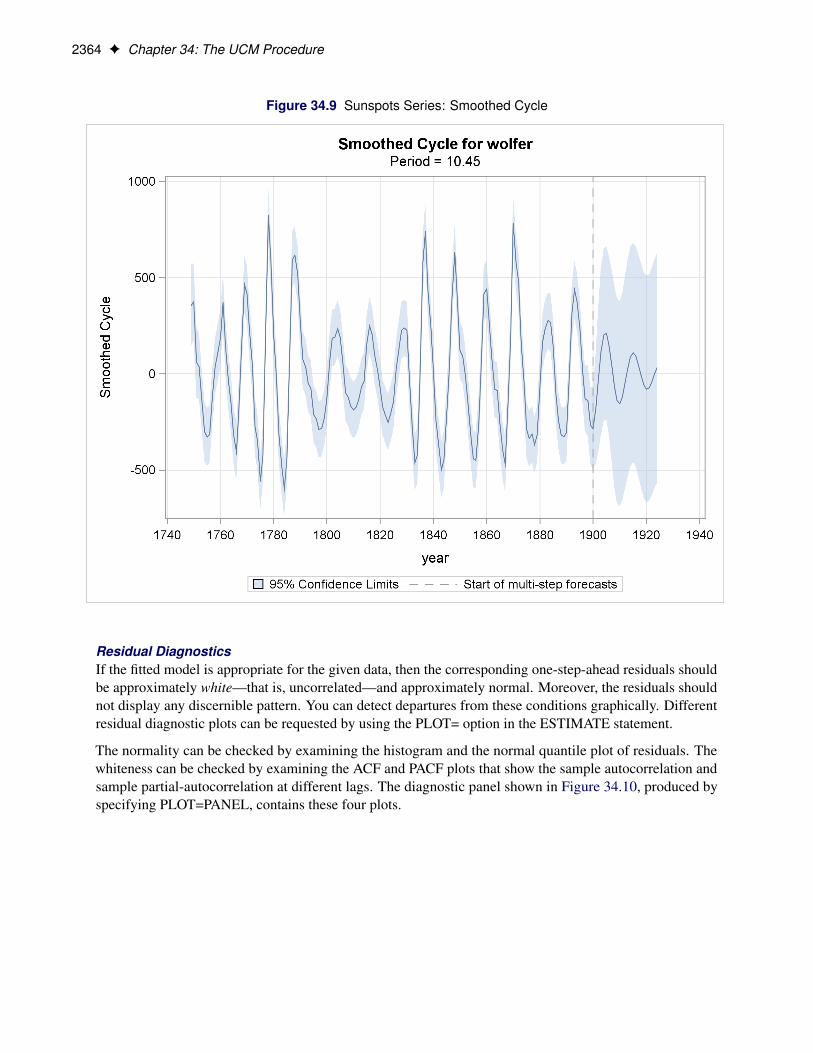
2364 F Chapter 34: The UCM Procedure
Figure 34.9 Sunspots Series: Smoothed Cycle
Residual DiagnosticsIf the fitted model is appropriate for the given data, then the corresponding one-step-ahead residuals shouldbe approximately white—that is, uncorrelated—and approximately normal. Moreover, the residuals shouldnot display any discernible pattern. You can detect departures from these conditions graphically. Differentresidual diagnostic plots can be requested by using the PLOT= option in the ESTIMATE statement.
The normality can be checked by examining the histogram and the normal quantile plot of residuals. Thewhiteness can be checked by examining the ACF and PACF plots that show the sample autocorrelation andsample partial-autocorrelation at different lags. The diagnostic panel shown in Figure 34.10, produced byspecifying PLOT=PANEL, contains these four plots.
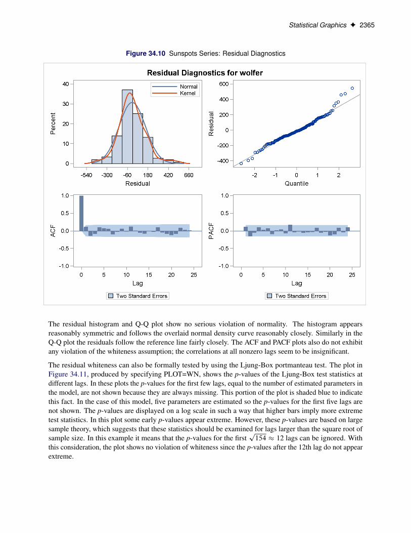
Statistical Graphics F 2365
Figure 34.10 Sunspots Series: Residual Diagnostics
The residual histogram and Q-Q plot show no serious violation of normality. The histogram appearsreasonably symmetric and follows the overlaid normal density curve reasonably closely. Similarly in theQ-Q plot the residuals follow the reference line fairly closely. The ACF and PACF plots also do not exhibitany violation of the whiteness assumption; the correlations at all nonzero lags seem to be insignificant.
The residual whiteness can also be formally tested by using the Ljung-Box portmanteau test. The plot inFigure 34.11, produced by specifying PLOT=WN, shows the p-values of the Ljung-Box test statistics atdifferent lags. In these plots the p-values for the first few lags, equal to the number of estimated parameters inthe model, are not shown because they are always missing. This portion of the plot is shaded blue to indicatethis fact. In the case of this model, five parameters are estimated so the p-values for the first five lags arenot shown. The p-values are displayed on a log scale in such a way that higher bars imply more extremetest statistics. In this plot some early p-values appear extreme. However, these p-values are based on largesample theory, which suggests that these statistics should be examined for lags larger than the square root ofsample size. In this example it means that the p-values for the first
p154 � 12 lags can be ignored. With
this consideration, the plot shows no violation of whiteness since the p-values after the 12th lag do not appearextreme.

2366 F Chapter 34: The UCM Procedure
Figure 34.11 Sunspots Series: Ljung-Box Portmanteau Test
The plot in Figure 34.12, produced by specifying PLOT=LOESS, shows the residuals plotted against timewith an overlaid LOESS curve. This plot is useful for checking whether any discernible pattern remains inthe residuals. Here again, no significant pattern appears to be present.

Statistical Graphics F 2367
Figure 34.12 Sunspots Series: Residual Loess Plot
The plot in Figure 34.13, produced by specifying PLOT=CUSUM, shows the cumulative residuals plottedagainst time. This plot is useful for checking structural breaks. Here, there appears to be no evidence ofstructural break since the cumulative residuals remain within the confidence band throughout the sampleperiod. Similarly you can request a plot of the squared cumulative residuals by specifying PLOT=CUSUMSQ.

2368 F Chapter 34: The UCM Procedure
Figure 34.13 Sunspots Series: CUSUM Plot
Brockwell and Davis (1991) can be consulted for additional information on diagnosing residuals. For moreinformation on CUSUM and CUSUMSQ plots, you can consult Harvey (1989).
Forecast and Series Decomposition PlotsYou can use the PLOT= option in the FORECAST statement to obtain the series forecast plot and theseries decomposition plots. The series decomposition plots show the result of successively adding differentcomponents in the model starting with the trend component. The IRREGULAR component is left out of thisprocess. The following two plots, produced by specifying PLOT=DECOMP, show the results of successivecomponent addition for this example. The first plot, shown in Figure 34.14, shows the smoothed trendcomponent and the second plot, shown in Figure 34.15, shows the sum of smoothed trend and cycle.
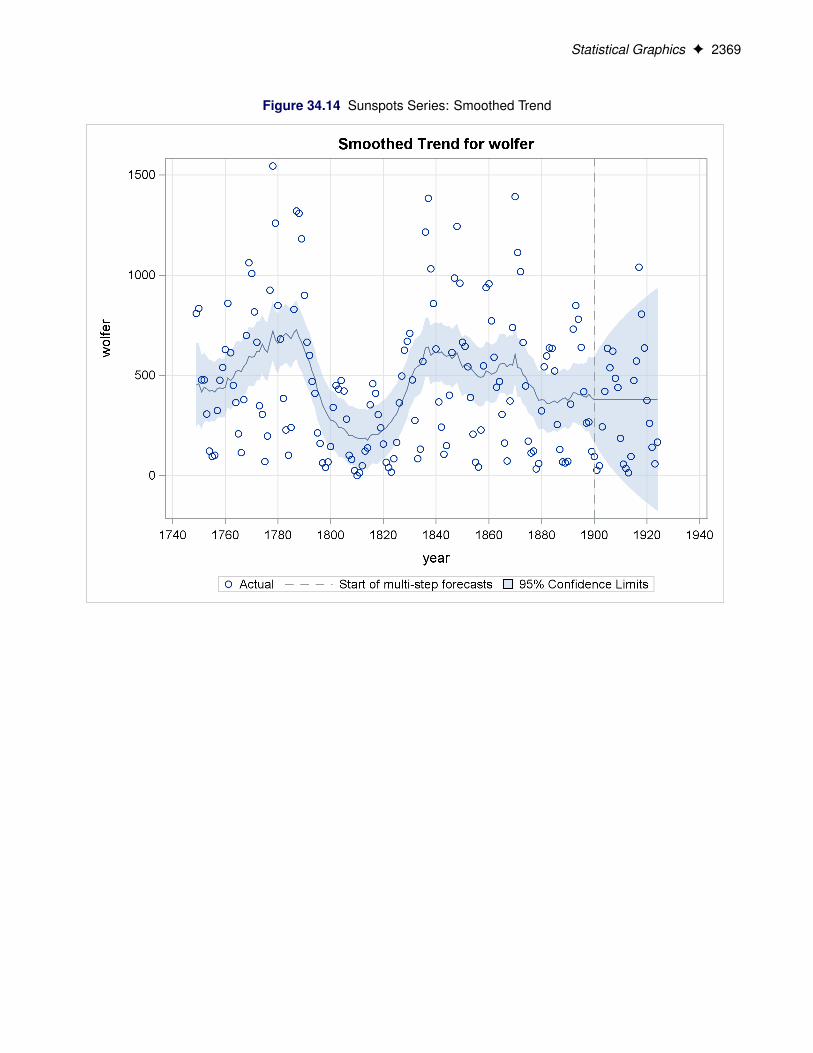
Statistical Graphics F 2369
Figure 34.14 Sunspots Series: Smoothed Trend
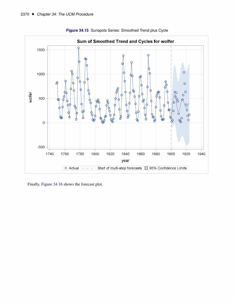
2370 F Chapter 34: The UCM Procedure
Figure 34.15 Sunspots Series: Smoothed Trend plus Cycle
Finally, Figure 34.16 shows the forecast plot.
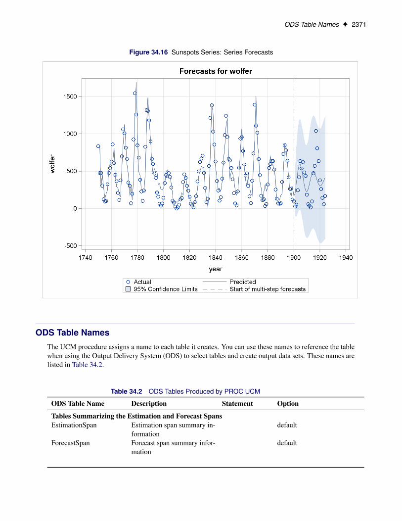
ODS Table Names F 2371
Figure 34.16 Sunspots Series: Series Forecasts
ODS Table NamesThe UCM procedure assigns a name to each table it creates. You can use these names to reference the tablewhen using the Output Delivery System (ODS) to select tables and create output data sets. These names arelisted in Table 34.2.
Table 34.2 ODS Tables Produced by PROC UCM
ODS Table Name Description Statement Option
Tables Summarizing the Estimation and Forecast SpansEstimationSpan Estimation span summary in-
formationdefault
ForecastSpan Forecast span summary infor-mation
default

2372 F Chapter 34: The UCM Procedure
Table 34.2 continued
ODS Table Name Description Statement Option
Tables Related to Model ParametersConvergenceStatus Convergence status of the es-
timation processdefault
FixedParameters Fixed parameters in themodel
default
InitialParameters Initial estimates of the freeparameters
default
ParameterEstimates Final estimates of the free pa-rameters
default
Tables Related to Model Information and DiagnosticsBlockSeasonDescription Information about the block
seasonals in the modeldefault
ComponentSignificance Significance analysis of thecomponents in the model
default
CycleDescription Information about the cyclesin the model
default
FitStatistics Fit statistics based on the one-step-ahead predictions
default
FitSummary Likelihood-based fit statistics defaultOutlierSummary Summary table of the de-
tected outliersdefault
SeasonDescription Information about the season-als in the model
default
SeasonHarmonics Summary of harmonics in atrigonometric seasonal com-ponent
SEASON PRINT=HARMONICS
SplineSeasonDescription Information about the spline-seasonals in the model
default
TrendInformation Summary information of thelevel and slope components
default
Tables Related to Filtered Component EstimatesFilteredAutoReg Filtered estimate of an au-
toreg componentAUTOREG PRINT=FILTER
FilteredBlockSeason Filtered estimate of a blockseasonal component
BLOCKSEASON PRINT=FILTER
FilteredCycle Filtered estimate of a cyclecomponent
CYCLE PRINT=FILTER
FilteredIrregular Filtered estimate of the irreg-ular component
IRREGULAR PRINT=FILTER
FilteredLevel Filtered estimate of the levelcomponent
LEVEL PRINT=FILTER

ODS Table Names F 2373
Table 34.2 continued
ODS Table Name Description Statement Option
FilteredRandomReg Filtered estimate of the time-varying random-regressioncoefficient
RANDOMREG PRINT=FILTER
FilteredSeason Filtered estimate of a sea-sonal component
SEASON PRINT=FILTER
FilteredSlope Filtered estimate of the slopecomponent
SLOPE PRINT=FILTER
FilteredSplineReg Filtered estimate of the time-varying spline-regression co-efficient
SPLINEREG PRINT=FILTER
FilteredSplineSeason Filtered estimate of a spline-seasonal component
SPLINESEASON PRINT=FILTER
Tables Related to Smoothed Component EstimatesSmoothedAutoReg Smoothed estimate of an au-
toreg componentAUTOREG PRINT=SMOOTH
SmoothedBlockSeason Smoothed estimate of a blockseasonal component
BLOCKSEASON PRINT=SMOOTH
SmoothedCycle Smoothed estimate of the cy-cle component
CYCLE PRINT=SMOOTH
SmoothedIrregular Smoothed estimate of the ir-regular component
IRREGULAR PRINT=SMOOTH
SmoothedLevel Smoothed estimate of thelevel component
LEVEL PRINT=SMOOTH
SmoothedRandomReg Smoothed estimate ofthe time-varying random-regression coefficient
RANDOMREG PRINT=SMOOTH
SmoothedSeason Smoothed estimate of a sea-sonal component
SEASON PRINT=SMOOTH
SmoothedSlope Smoothed estimate of theslope component
SLOPE PRINT=SMOOTH
SmoothedSplineReg Smoothed estimate ofthe time-varying spline-regression coefficient
SPLINEREG PRINT=SMOOTH
SmoothedSplineSeason Smoothed estimate of aspline-seasonal component
SPLINESEASON PRINT=SMOOTH
Tables Related to Series Decomposition and ForecastingFilteredAllExceptIrreg Filtered estimate of sum of all
components except the irreg-ular component
FORECAST PRINT=FDECOMP
FilteredTrend Filtered estimate of trend FORECAST PRINT= FDECOMP
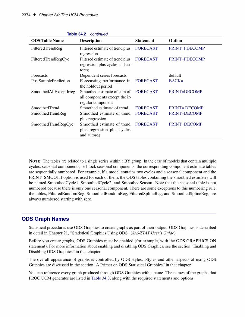
2374 F Chapter 34: The UCM Procedure
Table 34.2 continued
ODS Table Name Description Statement Option
FilteredTrendReg Filtered estimate of trend plusregression
FORECAST PRINT=FDECOMP
FilteredTrendRegCyc Filtered estimate of trend plusregression plus cycles and au-toreg
FORECAST PRINT=FDECOMP
Forecasts Dependent series forecasts defaultPostSamplePrediction Forecasting performance in
the holdout periodFORECAST BACK=
SmoothedAllExceptIrreg Smoothed estimate of sum ofall components except the ir-regular component
FORECAST PRINT=DECOMP
SmoothedTrend Smoothed estimate of trend FORECAST PRINT= DECOMPSmoothedTrendReg Smoothed estimate of trend
plus regressionFORECAST PRINT=DECOMP
SmoothedTrendRegCyc Smoothed estimate of trendplus regression plus cyclesand autoreg
FORECAST PRINT=DECOMP
NOTE: The tables are related to a single series within a BY group. In the case of models that contain multiplecycles, seasonal components, or block seasonal components, the corresponding component estimate tablesare sequentially numbered. For example, if a model contains two cycles and a seasonal component and thePRINT=SMOOTH option is used for each of them, the ODS tables containing the smoothed estimates willbe named SmoothedCycle1, SmoothedCycle2, and SmoothedSeason. Note that the seasonal table is notnumbered because there is only one seasonal component. There are some exceptions to this numbering rule:the tables, FilteredRandomReg, SmoothedRandomReg, FilteredSplineReg, and SmoothedSplineReg, arealways numbered starting with zero.
ODS Graph NamesStatistical procedures use ODS Graphics to create graphs as part of their output. ODS Graphics is describedin detail in Chapter 21, “Statistical Graphics Using ODS” (SAS/STAT User’s Guide).
Before you create graphs, ODS Graphics must be enabled (for example, with the ODS GRAPHICS ONstatement). For more information about enabling and disabling ODS Graphics, see the section “Enabling andDisabling ODS Graphics” in that chapter.
The overall appearance of graphs is controlled by ODS styles. Styles and other aspects of using ODSGraphics are discussed in the section “A Primer on ODS Statistical Graphics” in that chapter.
You can reference every graph produced through ODS Graphics with a name. The names of the graphs thatPROC UCM generates are listed in Table 34.3, along with the required statements and options.

ODS Graph Names F 2375
Table 34.3 ODS Graphics Produced by PROC UCM
ODS Graph Name Description Statement Option
Plots Related to Residual AnalysisErrorACFPlot Prediction error autocorrela-
tion plotESTIMATE PLOT=ACF
ErrorPACFPlot Prediction error partial-autocorrelation plot
ESTIMATE PLOT=PACF
ErrorHistogram Prediction error histogram ESTIMATE PLOT=NORMALErrorQQPlot Prediction error normal quan-
tile plotESTIMATE PLOT=QQ
ErrorPlot Plot of prediction errors ESTIMATE PLOT=RESIDUALErrorWhiteNoiseLogProbPlot Plot of p-values at differ-
ent lags for the Ljung-Boxportmanteau white noise teststatistics
ESTIMATE PLOT=WN
CUSUMPlot Plot of cumulative residuals ESTIMATE PLOT=CUSUMCUSUMSQPlot Plot of cumulative squared
residualsESTIMATE PLOT=CUSUMSQ
ModelPlot Plot of one-step-ahead fore-casts in the estimation span
ESTIMATE PLOT=MODEL
PanelResidualPlot Panel of residual diagnosticplots
ESTIMATE PLOT=PANEL
ResidualLoessPlot Time series plot of residualswith superimposed LOESSsmoother
ESTIMATE PLOT=LOESS
Plots Related to Filtered Component EstimatesFilteredAutoregPlot Plot of filtered autoreg com-
ponentAUTOREG PLOT=FILTER
FilteredBlockSeasonPlot Plot of filtered block seasoncomponent
BLOCKSEASON PLOT=FILTER
FilteredCyclePlot Plot of filtered cycle compo-nent
CYCLE PLOT=FILTER
FilteredIrregularPlot Plot of filtered irregular com-ponent
IRREGULAR PLOT=FILTER
FilteredLevelPlot Plot of filtered level compo-nent
LEVEL PLOT=FILTER
FilteredRandomRegPlot Plot of filtered time-varyingregression coefficient
RANDOMREG PLOT=FILTER
FilteredSeasonPlot Plot of filtered season compo-nent
SEASON PLOT=FILTER
FilteredSlopePlot Plot of filtered slope compo-nent
SLOPE PLOT=FILTER
FilteredSplineRegPlot Plot of filtered time-varyingregression coefficient
SPLINEREG PLOT=FILTER

2376 F Chapter 34: The UCM Procedure
Table 34.3 continued
ODS Graph Name Description Statement Option
FilteredSplineSeasonPlot Plot of filtered spline-seasoncomponent
SPLINESEASON PLOT=FILTER
AnnualSeasonPlot Plot of annual variation in thefiltered season component
SEASON PLOT=F_ANNUAL
Plots Related to Smoothed Component EstimatesSmoothedAutoregPlot Plot of smoothed autoreg
componentAUTOREG PLOT=SMOOTH
SmoothedBlockSeasonPlot Plot of smoothed block sea-son component
BLOCKSEASON PLOT=SMOOTH
SmoothedCyclePlot Plot of smoothed cycle com-ponent
CYCLE PLOT=SMOOTH
SmoothedIrregularPlot Plot of smoothed irregularcomponent
IRREGULAR PLOT=SMOOTH
SmoothedLevelPlot Plot of smoothed level com-ponent
LEVEL PLOT=SMOOTH
SmoothedRandomRegPlot Plot of smoothed time-varying regression coefficient
RANDOMREG PLOT=SMOOTH
SmoothedSeasonPlot Plot of smoothed season com-ponent
SEASON PLOT=SMOOTH
SmoothedSlopePlot Plot of smoothed slope com-ponent
SLOPE PLOT=SMOOTH
SmoothedSplineRegPlot Plot of smoothed time-varying regression coefficient
SPLINEREG PLOT=SMOOTH
SmoothedSplineSeasonPlot Plot of smoothed spline-season component
SPLINESEASON PLOT=SMOOTH
AnnualSeasonPlot Plot of annual variation in thesmoothed season component
SEASON PLOT=S_ANNUAL
Plots Related to Series Decomposition and ForecastingForecastsOnlyPlot Series forecasts beyond the
historical periodFORECAST DEFAULT
ForecastsPlot One-step-ahead as well asmultistep-ahead forecasts
FORECAST PLOT=FORECASTS
FilteredAllExceptIrregPlot Plot of sum of all filteredcomponents except the irreg-ular component
FORECAST PLOT= FDECOMP
FilteredTrendPlot Plot of filtered trend FORECAST PLOT= FDECOMP

ODS Graph Names F 2377
Table 34.3 continued
ODS Graph Name Description Statement Option
FilteredTrendRegCycPlot Plot of sum of filtered trend,cycles, and regression effects
FORECAST PLOT= FDECOMP
FilteredTrendRegPlot Plot of filtered trend plus re-gression effects
FORECAST PLOT= FDECOMP
SmoothedAllExceptIrregPlot Plot of sum of all smoothedcomponents except the irreg-ular component
FORECAST PLOT= DECOMP
SmoothedTrendPlot Plot of smoothed trend FORECAST PLOT= TRENDSmoothedTrendRegPlot Plot of smoothed trend plus
regression effectsFORECAST PLOT= DECOMP
SmoothedTrendRegCycPlot Plot of sum of smoothedtrend, cycles, and regressioneffects
FORECAST PLOT= DECOMP
FilteredAllExceptIrregVarPlot Plot of standard error of sumof all filtered components ex-cept the irregular
FORECAST PLOT= FDECOMPVAR
FilteredTrendVarPlot Plot of standard error of fil-tered trend
FORECAST PLOT= FDECOMPVAR
FilteredTrendRegVarPlot Plot of standard error of fil-tered trend plus regression ef-fects
FORECAST PLOT= FDECOMPVAR
FilteredTrendRegCycVarPlot Plot of standard error of fil-tered trend, cycles, and re-gression effects
FORECAST PLOT= FDECOMPVAR
SmoothedAllExceptIrregVarPlot Plot of standard error of sumof all smoothed componentsexcept the irregular
FORECAST PLOT= DECOMPVAR
SmoothedTrendVarPlot Plot of standard error ofsmoothed trend
FORECAST PLOT= DECOMPVAR
SmoothedTrendRegVarPlot Plot of standard error ofsmoothed trend plus regres-sion effects
FORECAST PLOT= DECOMPVAR
SmoothedTrendRegCycVarPlot Plot of standard error ofsmoothed trend, cycles, andregression effects
FORECAST PLOT= DECOMPVAR

2378 F Chapter 34: The UCM Procedure
OUTFOR= Data SetYou can use the OUTFOR= option in the FORECAST statement to store the series and component forecastsproduced by the procedure. This data set contains the following columns:
• the BY variables
• the ID variable. If an ID variable is not specified, then a numerical variable, _ID_, is created thatcontains the observation numbers from the input data set.
• the dependent series and the predictor series
• FORECAST, a numerical variable containing the one-step-ahead predicted values and the multistepforecasts
• RESIDUAL, a numerical variable containing the difference between the actual and forecast values
• STD, a numerical variable containing the standard error of prediction
• LCL and UCL, numerical variables containing the lower and upper forecast confidence limits
• S_SERIES and VS_SERIES, numerical variables containing the smoothed values of the dependentseries and their variances
• S_IRREG and VS_IRREG, numerical variables containing the smoothed values of the irregular com-ponent and their variances. These variables are present only if the model has an irregular component.
• F_LEVEL, VF_LEVEL, S_LEVEL, and VS_LEVEL, numerical variables containing the filtered andsmoothed values of the level component and the respective variances. These variables are present onlyif the model has a level component.
• F_SLOPE, VF_SLOPE, S_SLOPE, and VS_SLOPE, numerical variables containing the filtered andsmoothed values of the slope component and the respective variances. These variables are present onlyif the model has a slope component.
• F_AUTOREG, VF_AUTOREG, S_AUTOREG, and VS_AUTOREG, numerical variables containingthe filtered and smoothed values of the autoreg component and the respective variances. These variablesare present only if the model has an autoreg component.
• F_CYCLE, VF_CYCLE, S_CYCLE, and VS_CYCLE, numerical variables containing the filtered andsmoothed values of the cycle component and the respective variances. If there are multiple cycles inthe model, these variables are sequentially numbered as F_CYCLE1, F_CYCLE2, etc. These variablesare present only if the model has at least one cycle component.
• F_SEASON, VF_SEASON, S_SEASON, and VS_SEASON, numerical variables containing thefiltered and smoothed values of the season component and the respective variances. If there are multipleseasons in the model, these variables are sequentially numbered as F_SEASON1, F_SEASON2, etc.These variables are present only if the model has at least one season component.
• F_BLKSEAS, VF_BLKSEAS, S_BLKSEAS, and VS_BLKSEAS, numerical variables containingthe filtered and smoothed values of the blockseason component and the respective variances. If thereare multiple block seasons in the model, these variables are sequentially numbered as F_BLKSEAS1,F_BLKSEAS2, etc.

OUTEST= Data Set F 2379
• F_SPLSEAS, VF_SPLSEAS, S_SPLSEAS, and VS_SPLSEAS, numerical variables containing thefiltered and smoothed values of the splineseason component and the respective variances. If thereare multiple spline seasons in the model, these variables are sequentially numbered as F_SPLSEAS1,F_SPLSEAS2, etc. These variables are present only if the model has at least one splineseasoncomponent.
• Filtered and smoothed estimates, and their variances, of the time-varying regression coefficients of thevariables specified in the RANDOMREG and SPLINEREG statements. A variable is not included ifits coefficient is time-invariant, that is, if the associated disturbance variance is zero.
• S_TREG and VS_TREG, numerical variables containing the smoothed values of level plus regressioncomponent and their variances. These variables are present only if the model has at least one predictorvariable or has dependent lags.
• S_TREGCYC and VS_TREGCYC, numerical variables containing the smoothed values of level plusregression plus cycle component and their variances. These variables are present only if the model hasat least one cycle or an autoreg component.
• S_NOIRREG and VS_NOIRREG, numerical variables containing the smoothed values of the sum ofall components except the irregular component and their variances. These variables are present only ifthe model has at least one seasonal or block seasonal component.
OUTEST= Data SetYou can use the OUTEST= option in the ESTIMATE statement to store the model parameters and the relatedestimation details. This data set contains the following columns:
• the BY variables
• COMPONENT, a character variable containing the name of the component corresponding to theparameter being described
• PARAMETER, a character variable containing the parameter name
• TYPE, a character variable indicating whether the parameter value was fixed by the user or estimated
• _STATUS_, a character variable indicating whether the parameter estimation process converged orfailed or there was an error of some other kind
• ESTIMATE, a numerical variable containing the parameter estimate
• STD, a numerical variable containing the standard error of the parameter estimate. This has a missingvalue if the parameter value is fixed.
• TVALUE, a numerical variable containing the t-statistic. This has a missing value if the parametervalue is fixed.
• PVALUE, a numerical variable containing the p-value. This has a missing value if the parameter valueis fixed.

2380 F Chapter 34: The UCM Procedure
Statistics of FitThis section explains the goodness-of-fit statistics reported to measure how well the specified model fits thedata.
First the various statistics of fit that are computed using the prediction errors, yt � Oyt , are considered. Inthese formulas, n is the number of nonmissing prediction errors and k is the number of fitted parameters inthe model. Moreover, the sum of squared errors, SSE D
P.yt � Oyt /
2, and the total sum of squares for theseries corrected for the mean, SST D
P.yt � y/
2, where y is the series mean, and the sums are over allthe nonmissing prediction errors.
Mean Squared ErrorThe mean squared prediction error, MSE D 1
nSSE
Root Mean Squared ErrorThe root mean square error, RMSE =
pMSE
Mean Absolute Percent ErrorThe mean absolute percent prediction error, MAPE = 100
n
PntD1 j.yt � Oyt /=yt j.
The summation ignores observations where yt D 0.
R-squareThe R-square statistic, R2 D 1 � SSE=SST .If the model fits the series badly, the model error sum of squares, SSE, might be larger than SST and theR-square statistic will be negative.
Adjusted R-squareThe adjusted R-square statistic, 1 � .n�1
n�k/.1 � R2/
Amemiya’s Adjusted R-squareAmemiya’s adjusted R-square, 1 � .nCk
n�k/.1 � R2/
Random Walk R-squareThe random walk R-square statistic (Harvey’s R-square statistic that uses the random walkmodel for comparison), 1 � .n�1
n/SSE=RWSSE , where RWSSE D
PntD2 .yt � yt�1 � �/
2, and� D 1
n�1
PntD2 .yt � yt�1/
Maximum Percent ErrorThe largest percent prediction error, 100 max..yt � Oyt /=yt /. In this computation the observations whereyt D 0 are ignored.
The likelihood-based fit statistics are reported separately (see the section “The UCMs as State Space Models”on page 2347). They include the full log likelihood (L1), the diffuse part of the log likelihood, the normalizedresidual sum of squares, and several information criteria: AIC, AICC, HQIC, BIC, and CAIC. Let q denote thenumber of estimated parameters, n be the number of nonmissing measurements in the estimation span, and dbe the number of diffuse elements in the initial state vector that are successfully initialized during the Kalmanfiltering process. Moreover, let n� D .n� d/. The reported information criteria, all in smaller-is-better form,are described in Table 34.4:
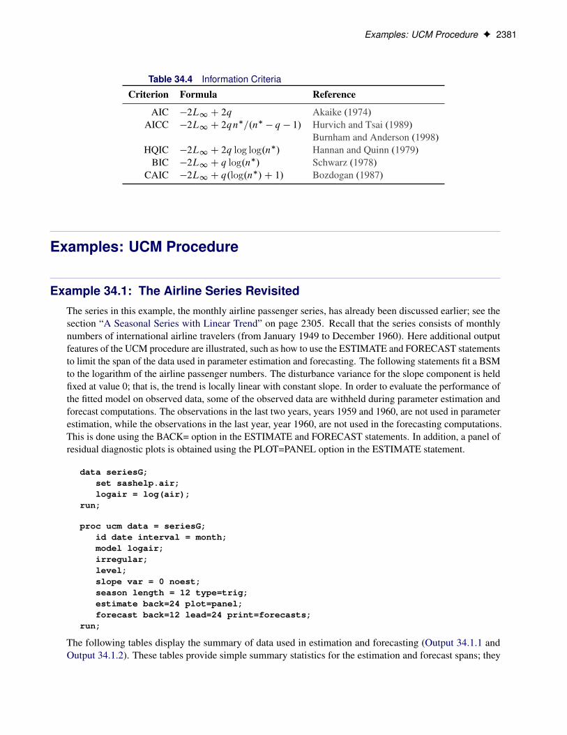
Examples: UCM Procedure F 2381
Table 34.4 Information Criteria
Criterion Formula Reference
AIC �2L1 C 2q Akaike (1974)AICC �2L1 C 2qn
�=.n� � q � 1/ Hurvich and Tsai (1989)Burnham and Anderson (1998)
HQIC �2L1 C 2q log log.n�/ Hannan and Quinn (1979)BIC �2L1 C q log.n�/ Schwarz (1978)
CAIC �2L1 C q.log.n�/C 1/ Bozdogan (1987)
Examples: UCM Procedure
Example 34.1: The Airline Series RevisitedThe series in this example, the monthly airline passenger series, has already been discussed earlier; see thesection “A Seasonal Series with Linear Trend” on page 2305. Recall that the series consists of monthlynumbers of international airline travelers (from January 1949 to December 1960). Here additional outputfeatures of the UCM procedure are illustrated, such as how to use the ESTIMATE and FORECAST statementsto limit the span of the data used in parameter estimation and forecasting. The following statements fit a BSMto the logarithm of the airline passenger numbers. The disturbance variance for the slope component is heldfixed at value 0; that is, the trend is locally linear with constant slope. In order to evaluate the performance ofthe fitted model on observed data, some of the observed data are withheld during parameter estimation andforecast computations. The observations in the last two years, years 1959 and 1960, are not used in parameterestimation, while the observations in the last year, year 1960, are not used in the forecasting computations.This is done using the BACK= option in the ESTIMATE and FORECAST statements. In addition, a panel ofresidual diagnostic plots is obtained using the PLOT=PANEL option in the ESTIMATE statement.
data seriesG;set sashelp.air;logair = log(air);
run;
proc ucm data = seriesG;id date interval = month;model logair;irregular;level;slope var = 0 noest;season length = 12 type=trig;estimate back=24 plot=panel;forecast back=12 lead=24 print=forecasts;
run;
The following tables display the summary of data used in estimation and forecasting (Output 34.1.1 andOutput 34.1.2). These tables provide simple summary statistics for the estimation and forecast spans; they
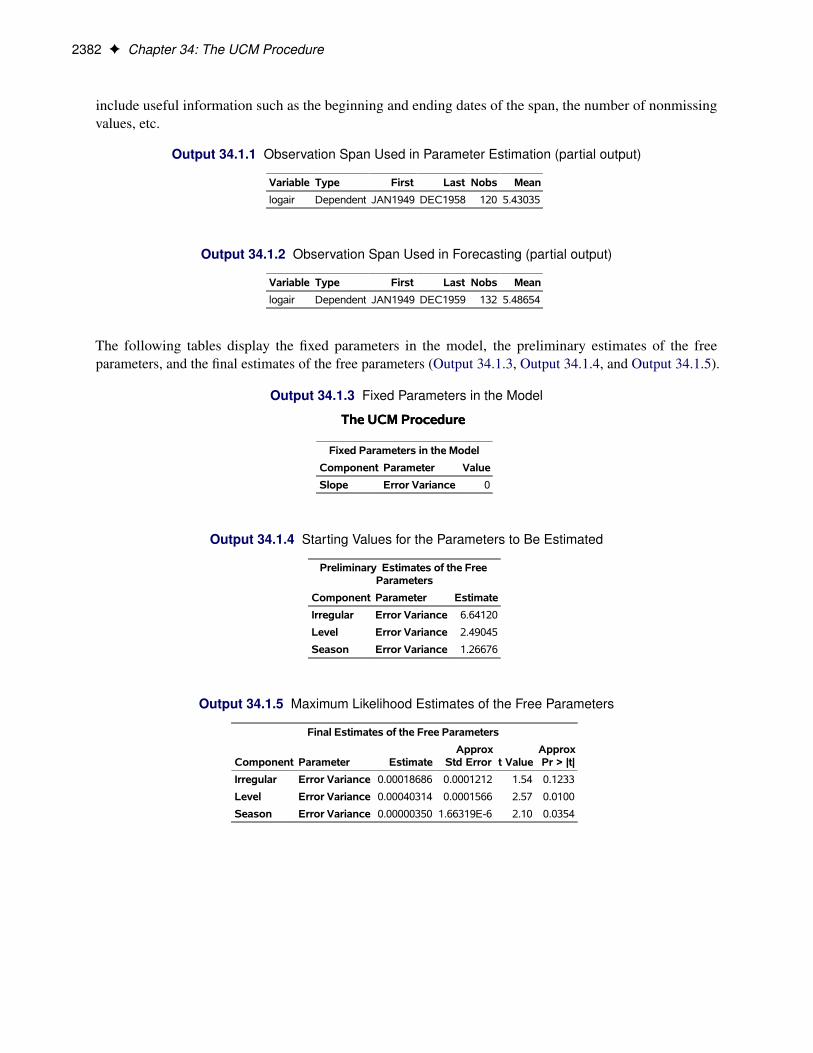
2382 F Chapter 34: The UCM Procedure
include useful information such as the beginning and ending dates of the span, the number of nonmissingvalues, etc.
Output 34.1.1 Observation Span Used in Parameter Estimation (partial output)
Variable Type First Last Nobs Mean
logair Dependent JAN1949 DEC1958 120 5.43035
Output 34.1.2 Observation Span Used in Forecasting (partial output)
Variable Type First Last Nobs Mean
logair Dependent JAN1949 DEC1959 132 5.48654
The following tables display the fixed parameters in the model, the preliminary estimates of the freeparameters, and the final estimates of the free parameters (Output 34.1.3, Output 34.1.4, and Output 34.1.5).
Output 34.1.3 Fixed Parameters in the Model
The UCM ProcedureThe UCM Procedure
Fixed Parameters in the Model
Component Parameter Value
Slope Error Variance 0
Output 34.1.4 Starting Values for the Parameters to Be Estimated
Preliminary Estimates of the FreeParameters
Component Parameter Estimate
Irregular Error Variance 6.64120
Level Error Variance 2.49045
Season Error Variance 1.26676
Output 34.1.5 Maximum Likelihood Estimates of the Free Parameters
Final Estimates of the Free Parameters
Component Parameter EstimateApprox
Std Error t ValueApproxPr > |t|
Irregular Error Variance 0.00018686 0.0001212 1.54 0.1233
Level Error Variance 0.00040314 0.0001566 2.57 0.0100
Season Error Variance 0.00000350 1.66319E-6 2.10 0.0354

Example 34.1: The Airline Series Revisited F 2383
Two types of goodness-of-fit statistics are reported after a model is fit to the series (see Output 34.1.6and Output 34.1.7). The first type is the likelihood-based goodness-of-fit statistics, which include the fulllikelihood of the data, the diffuse portion of the likelihood (see the section “Details: UCM Procedure” onpage 2342), and the information criteria. The second type of statistics is based on the raw residuals, residual= observed – predicted. If the model is nonstationary, then one-step-ahead predictions are not available forsome initial observations, and the number of values used in computing these fit statistics will be differentfrom those used in computing the likelihood-based test statistics.
Output 34.1.6 Likelihood-Based Fit Statistics for the Airline Data
Likelihood Based Fit Statistics
Statistic Value
Full Log Likelihood 180.63
Diffuse Part of Log Likelihood -13.93
Non-Missing Observations Used 120
Estimated Parameters 3
Initialized Diffuse State Elements 13
Normalized Residual Sum of Squares 107
AIC (smaller is better) -355.3
BIC (smaller is better) -347.2
AICC (smaller is better) -355
HQIC (smaller is better) -352
CAIC (smaller is better) -344.2
Output 34.1.7 Residuals-Based Fit Statistics for the Airline Data
Fit Statistics Based on Residuals
Mean Squared Error 0.00156
Root Mean Squared Error 0.03944
Mean Absolute Percentage Error 0.57677
Maximum Percent Error 2.19396
R-Square 0.98705
Adjusted R-Square 0.98680
Random Walk R-Square 0.86370
Amemiya's Adjusted R-Square 0.98630
Number of non-missing residuals usedfor computing the fit statistics = 107
The diagnostic plots based on the one-step-ahead residuals are shown in Output 34.1.8. The residual histogramand the Q-Q plot show no reasons to question the approximate normality of the residual distribution. Theremaining plots check for the whiteness of the residuals. The sample correlation plots, the autocorrelationfunction (ACF) and the partial autocorrelation function (PACF), also do not show any significant violationsof the whiteness of the residuals. Therefore, on the whole, the model seems to fit the data well.

2384 F Chapter 34: The UCM Procedure
Output 34.1.8 Residual Diagnostics for the Airline Series Using a BSM
The forecasts are given in Output 34.1.9. In order to save the space, the upper and lower confidence limitcolumns are dropped from the output, and only the rows corresponding to the year 1960 are shown. Recallthat the actual measurements in the years 1959 and 1960 were withheld during the parameter estimation, andthe ones in 1960 were not used in the forecast computations.

Example 34.1: The Airline Series Revisited F 2385
Output 34.1.9 continued
Output 34.1.9 Forecasts for the Airline Data
Obs date Forecast StdErr logair Residual
133 JAN60 6.050 0.038 6.033 -0.017
134 FEB60 5.996 0.044 5.969 -0.027
135 MAR60 6.156 0.049 6.038 -0.118
136 APR60 6.124 0.053 6.133 0.010
137 MAY60 6.168 0.058 6.157 -0.011
138 JUN60 6.303 0.061 6.282 -0.021
139 JUL60 6.435 0.065 6.433 -0.002
140 AUG60 6.450 0.068 6.407 -0.043
141 SEP60 6.265 0.071 6.230 -0.035
142 OCT60 6.138 0.073 6.133 -0.005
143 NOV60 6.015 0.075 5.966 -0.049
144 DEC60 6.121 0.077 6.068 -0.053
The figure Output 34.1.10 shows the forecast plot. The forecasts in the year 1960 show that the modelpredictions were quite good.

2386 F Chapter 34: The UCM Procedure
Output 34.1.10 Forecast Plot of the Airline Series Using a BSM
Example 34.2: Variable Star DataThe series in this example is studied in detail in Bloomfield (2000). This series consists of bright-ness measurements (magnitude) of a variable star taken at midnight for 600 consecutive days. Thedata can be downloaded from a time series archive maintained by the University of York, England(http://www.york.ac.uk/depts/maths/data/ts/welcome.htm (series number 26)). The following DATA stepstatements read the data in a SAS data set.
data star;input magnitude @@;day = _n_;
datalines;25 28 31 32 33 33 32 31 28 25 22 1814 10 7 4 2 0 0 0 2 4 8 1115 19 23 26 29 32 33 34 33 32 30 2724 20 17 13 10 7 5 3 3 3 4 57 10 13 16 19 22 24 26 27 28 29 2827 25 24 21 19 17 15 13 12 11 11 1010 11 12 12 13 14 15 16 17 18 19 19
... more lines ...
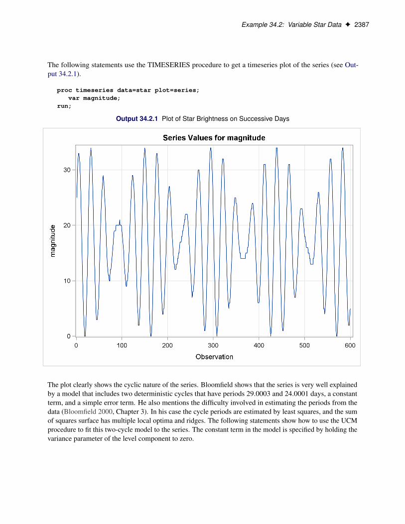
Example 34.2: Variable Star Data F 2387
The following statements use the TIMESERIES procedure to get a timeseries plot of the series (see Out-put 34.2.1).
proc timeseries data=star plot=series;var magnitude;
run;
Output 34.2.1 Plot of Star Brightness on Successive Days
The plot clearly shows the cyclic nature of the series. Bloomfield shows that the series is very well explainedby a model that includes two deterministic cycles that have periods 29.0003 and 24.0001 days, a constantterm, and a simple error term. He also mentions the difficulty involved in estimating the periods from thedata (Bloomfield 2000, Chapter 3). In his case the cycle periods are estimated by least squares, and the sumof squares surface has multiple local optima and ridges. The following statements show how to use the UCMprocedure to fit this two-cycle model to the series. The constant term in the model is specified by holding thevariance parameter of the level component to zero.

2388 F Chapter 34: The UCM Procedure
proc ucm data=star;model magnitude;irregular;level var=0 noest;cycle;cycle;estimate;
run;
The final parameter estimates and the goodness-of-fit statistics are shown in Output 34.2.2 and Output 34.2.3,respectively. The model fit appears to be good.
Output 34.2.2 Two-Cycle Model: Parameter Estimates
The UCM ProcedureThe UCM Procedure
Final Estimates of the Free Parameters
Component Parameter EstimateApprox
Std Error t ValueApproxPr > |t|
Irregular Error Variance 0.09257 0.0053845 17.19 <.0001
Cycle_1 Damping Factor 1.00000 1.81175E-7 5519514 <.0001
Cycle_1 Period 29.00036 0.0022709 12770.4 <.0001
Cycle_1 Error Variance 0.00000882 5.27213E-6 1.67 0.0944
Cycle_2 Damping Factor 1.00000 2.11939E-7 4718334 <.0001
Cycle_2 Period 24.00011 0.0019128 12547.2 <.0001
Cycle_2 Error Variance 0.00000535 3.56374E-6 1.50 0.1330
Output 34.2.3 Two-Cycle Model: Goodness of Fit
Fit Statistics Based on Residuals
Mean Squared Error 0.12072
Root Mean Squared Error 0.34745
Mean Absolute Percentage Error 2.65141
Maximum Percent Error 36.38991
R-Square 0.99850
Adjusted R-Square 0.99849
Random Walk R-Square 0.97281
Amemiya's Adjusted R-Square 0.99847
Number of non-missing residuals used forcomputing the fit statistics = 599
A summary of the cycles in the model is given in Output 34.2.4.
Output 34.2.4 Two-Cycle Model: Summary
Name Type period Rho ErrorVar
Cycle_1 Stationary 29.00036 1.00000 0.00000882
Cycle_2 Stationary 24.00011 1.00000 0.00000535

Example 34.3: Modeling Long Seasonal Patterns F 2389
Note that the estimated periods are the same as in Bloomfield’s model, the damping factors are nearly equalto 1.0, and the disturbance variances are very close to zero, implying persistent deterministic cycles. In fact,this model is identical to Bloomfield’s model.
Example 34.3: Modeling Long Seasonal PatternsThis example illustrates some of the techniques you can use to model long seasonal patterns in a series. If theseasonal pattern is of moderate length and the underlying dynamics are simple, then it is easily modeled byusing the basic settings of the SEASON statement and these additional techniques are not needed. However,if the seasonal pattern has a long season length and/or has a complex stochastic dynamics, then the techniquesdiscussed here can be useful. You can obtain parsimonious models for a long seasonal pattern by usingan appropriate subset of trigonometric harmonics, or by using a suitable spline function, or by using ablock-season pattern in combination with a seasonal component of much smaller length. You can also varythe disturbance variances of the subcomponents that combine to form the seasonal component.
The time series used in this example consists of number of calls received per shift at a call center. Eachshift is six hours long, and the first shift of the day begins at midnight, resulting in four shifts per day. Theobservations are available from December 15, 1999, to April 30, 2000. This series is seasonal with seasonlength 28, which is moderate, and in fact there is no particular need to use pattern approximation techniquesin this case. However, it is adequate for demonstration purposes. The plan of this example is as follows. Firstan initial model with a full seasonal component is created. This model is used as a baseline for comparingalternate models created by the techniques that are being illustrated. In practice any candidate model is firstchecked for adequacy by using various diagnostic procedures. In this illustration the main focus is on thedifferent ways a long seasonal pattern can be modeled and no model diagnostics are done for the modelsbeing entertained. The alternate models are compared by using the sum of absolute prediction errors in theholdout region.
The following DATA step statements create the input data set used in this example.
data callCenter;input calls @@;label calls= "Number of Calls Received in a 6 Hour Shift";start = '15dec99:00:00'dt;datetime = INTNX( 'dthour6', start, _n_-1 );format datetime datetime10.;
datalines;18 122 244 128 19 113 230 119 17 112
219 93 14 73 139 53 11 32 74 5615 137 289 153 20 125 227 106 16 101
201 92 14 94 187 69 11 59 94 21
... more lines ...
Initial exploration of the series clearly indicates that the series does not show any significant trend, and timeof day and day of the week have a significant influence on the number of calls received. These considerationssuggest a simple random walk trend model along with a seasonal component of season length 28, the totalnumber of shifts in a week. The following statements specify this model. Note the PRINT=HARMONICSoption in the SEASON statement, which produces a table that lists the full set of harmonics contributing tothe seasonal along with the significance of their contribution. This table will be useful later in choosing a

2390 F Chapter 34: The UCM Procedure
subset trigonometric model. The BACK=28 and the LEAD=28 specifications in the FORECAST statementcreate a holdout region of 28 observations. The sum of absolute prediction errors (SAE) in this holdoutregion are used to compare the different models.
proc ucm data=callCenter;id datetime interval=dthour6;model calls;irregular;level;season length=28 type=trig
print=(harmonics);estimate back=28;forecast back=28 lead=28;
run;
The forecasting performance of this model in the holdout region is shown in Output 34.3.1. The sum ofabsolute prediction errors SAE = 516.22, which appears in the last row of the holdout analysis table.
Output 34.3.1 Predictions in the Holdout Region: Baseline Model
Obs datetime Actual Forecast Error SAE
525 24APR00:00 12 -4.004 16.004 16.004
526 24APR00:06 136 110.825 25.175 41.179
527 24APR00:12 295 262.820 32.180 73.360
528 24APR00:18 172 145.127 26.873 100.232
529 25APR00:00 20 2.188 17.812 118.044
530 25APR00:06 127 105.442 21.558 139.602
531 25APR00:12 236 217.043 18.957 158.559
532 25APR00:18 125 114.313 10.687 169.246
533 26APR00:00 16 2.855 13.145 182.391
534 26APR00:06 108 95.202 12.798 195.189
535 26APR00:12 207 194.184 12.816 208.005
536 26APR00:18 112 97.687 14.313 222.317
537 27APR00:00 15 1.270 13.730 236.047
538 27APR00:06 98 85.875 12.125 248.172
539 27APR00:12 200 184.891 15.109 263.281
540 27APR00:18 113 93.113 19.887 283.168
541 28APR00:00 15 -1.120 16.120 299.288
542 28APR00:06 104 84.983 19.017 318.305
543 28APR00:12 205 177.940 27.060 345.365
544 28APR00:18 89 64.292 24.708 370.073
545 29APR00:00 12 -6.020 18.020 388.093
546 29APR00:06 68 46.286 21.714 409.807
547 29APR00:12 116 100.339 15.661 425.468
548 29APR00:18 54 34.700 19.300 444.768
549 30APR00:00 10 -6.209 16.209 460.978
550 30APR00:06 30 12.167 17.833 478.811
551 30APR00:12 66 49.524 16.476 495.287
552 30APR00:18 61 40.071 20.929 516.216

Example 34.3: Modeling Long Seasonal Patterns F 2391
Now that a baseline model is created, the exploration for alternate models can begin. The review of theharmonic table in Output 34.3.2 shows that all but the last three harmonics are significant, and deletingany of them to form a subset trigonometric seasonal component will lead to a poorer model. The last threeharmonics, 12th, 13th and 14th, with periods of 2.333, 2.15 and 2.0, respectively, do appear to be possiblechoices for deletion. Note that the disturbance variance of the seasonal component is not very insignificant(see Output 34.3.3); therefore the seasonal component is stochastic and the preceding logic, which is basedon the final state estimate, provides only a rough guideline.
Output 34.3.2 Harmonic Analysis of the Season: Initial Model
The UCM ProcedureThe UCM Procedure
Harmonic Analysis of Trigonometric Seasons(Based on the Final State)
NameSeasonLength Harmonic Period Chi-Square DF Pr > ChiSq
Season 28 1 28.00000 234.19 2 <.0001
Season 28 2 14.00000 264.19 2 <.0001
Season 28 3 9.33333 95.65 2 <.0001
Season 28 4 7.00000 105.64 2 <.0001
Season 28 5 5.60000 146.74 2 <.0001
Season 28 6 4.66667 121.93 2 <.0001
Season 28 7 4.00000 4299.12 2 <.0001
Season 28 8 3.50000 150.79 2 <.0001
Season 28 9 3.11111 89.68 2 <.0001
Season 28 10 2.80000 8.95 2 0.0114
Season 28 11 2.54545 6.14 2 0.0464
Season 28 12 2.33333 2.20 2 0.3325
Season 28 13 2.15385 3.40 2 0.1828
Season 28 14 2.00000 2.33 1 0.1272
Output 34.3.3 Parameter Estimates: Initial Model
Final Estimates of the Free Parameters
Component Parameter EstimateApprox
Std Error t ValueApproxPr > |t|
Irregular Error Variance 92.14591 13.10986 7.03 <.0001
Level Error Variance 44.83595 10.65465 4.21 <.0001
Season Error Variance 0.01250 0.0065153 1.92 0.0551
The following statements fit a subset trigonometric model formed by dropping the last three harmonics byspecifying the DROPH= option in the SEASON statement:
proc ucm data=callCenter;id datetime interval=dthour6;model calls;irregular;level;season length=28 type=trig droph=12 13 14;estimate back=28;forecast back=28 lead=28;
run;
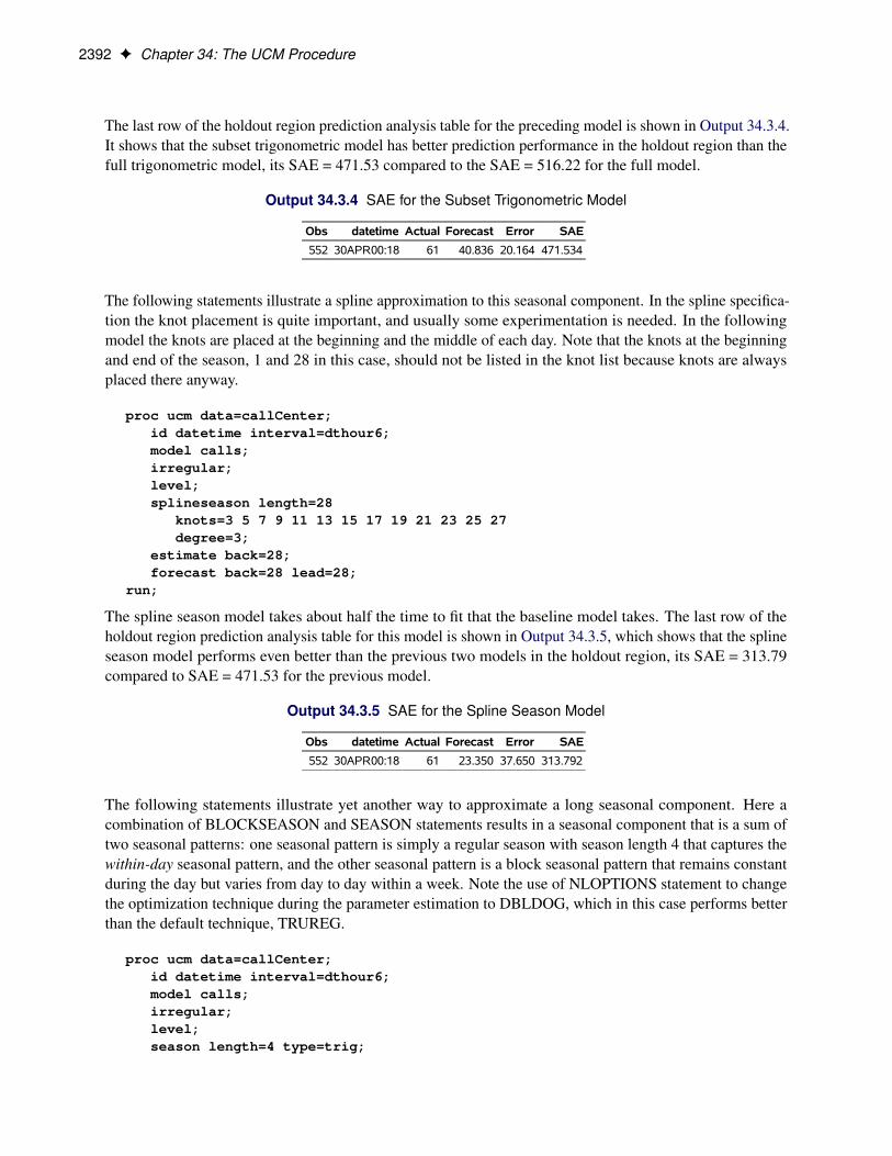
2392 F Chapter 34: The UCM Procedure
The last row of the holdout region prediction analysis table for the preceding model is shown in Output 34.3.4.It shows that the subset trigonometric model has better prediction performance in the holdout region than thefull trigonometric model, its SAE = 471.53 compared to the SAE = 516.22 for the full model.
Output 34.3.4 SAE for the Subset Trigonometric Model
Obs datetime Actual Forecast Error SAE
552 30APR00:18 61 40.836 20.164 471.534
The following statements illustrate a spline approximation to this seasonal component. In the spline specifica-tion the knot placement is quite important, and usually some experimentation is needed. In the followingmodel the knots are placed at the beginning and the middle of each day. Note that the knots at the beginningand end of the season, 1 and 28 in this case, should not be listed in the knot list because knots are alwaysplaced there anyway.
proc ucm data=callCenter;id datetime interval=dthour6;model calls;irregular;level;splineseason length=28
knots=3 5 7 9 11 13 15 17 19 21 23 25 27degree=3;
estimate back=28;forecast back=28 lead=28;
run;
The spline season model takes about half the time to fit that the baseline model takes. The last row of theholdout region prediction analysis table for this model is shown in Output 34.3.5, which shows that the splineseason model performs even better than the previous two models in the holdout region, its SAE = 313.79compared to SAE = 471.53 for the previous model.
Output 34.3.5 SAE for the Spline Season Model
Obs datetime Actual Forecast Error SAE
552 30APR00:18 61 23.350 37.650 313.792
The following statements illustrate yet another way to approximate a long seasonal component. Here acombination of BLOCKSEASON and SEASON statements results in a seasonal component that is a sum oftwo seasonal patterns: one seasonal pattern is simply a regular season with season length 4 that captures thewithin-day seasonal pattern, and the other seasonal pattern is a block seasonal pattern that remains constantduring the day but varies from day to day within a week. Note the use of NLOPTIONS statement to changethe optimization technique during the parameter estimation to DBLDOG, which in this case performs betterthan the default technique, TRUREG.
proc ucm data=callCenter;id datetime interval=dthour6;model calls;irregular;level;season length=4 type=trig;

Example 34.4: Modeling Time-Varying Regression Effects F 2393
blockseason nblocks=7 blocksize=4type=trig;
estimate back=28;forecast back=28 lead=28;nloptions tech=dbldog;
run;
This model also takes about half the time to fit that the baseline model takes. The last row of the holdoutregion prediction analysis table for this model is shown in Output 34.3.6, which shows that the block seasonmodel does slightly better than the baseline model but not as good as the other two models, its SAE = 508.52compared to the SAE = 516.22 of the baseline model.
Output 34.3.6 SAE for the Block Season Model
Obs datetime Actual Forecast Error SAE
552 30APR00:18 61 39.339 21.661 508.522
This example showed a few different ways to model a long seasonal pattern. It showed that parsimoniousmodels for long seasonal patterns can be useful, and in some cases even more effective than the full model.Moreover, for very long seasonal patterns the high memory requirements and long computing times mightmake full models impractical.
Example 34.4: Modeling Time-Varying Regression EffectsIn April 1979 the Albuquerque Police Department began a special enforcement program aimed at reducingthe number of DWI (driving while intoxicated) accidents. The program was administered by a squadof police officers, who used breath alcohol testing (BAT) devices and a van that houses a BAT device(Batmobile). These data were collected by the Division of Governmental Research of the University of NewMexico, under a contract with the National Highway Traffic Safety Administration of the U.S. Departmentof Transportation, to evaluate the Batmobile program. The first 29 observations are for a control period,and the next 23 observations are for the experimental (Batmobile) period. The data, freely available athttp://lib.stat.cmu.edu/DASL/Datafiles/batdat.html, consist of two variables: ACC, which represents injuriesand fatalities from Wednesday to Saturday nighttime accidents, and FUEL, which represents fuel consumption(millions of gallons) in Albuquerque. The variables are measured quarterly starting from the first quarterof 1972 up to the last quarter of 1984, covering the span of 13 years. The following DATA step statementscreate the input data set.
data bat;input ACC FUEL @@;batProgram = 0;if _n_ > 29 then batProgram = 1;date = INTNX( 'qtr', '1jan1972'd, _n_- 1 );format date qtr8.;
datalines;192 32.592 238 37.250 232 40.032246 35.852 185 38.226 274 38.711266 43.139 196 40.434 170 35.898234 37.111 272 38.944 234 37.717210 37.861 280 42.524 246 43.965248 41.976 269 42.918 326 49.789

2394 F Chapter 34: The UCM Procedure
342 48.454 257 45.056 280 49.385290 42.524 356 51.224 295 48.562279 48.167 330 51.362 354 54.646331 53.398 291 50.584 377 51.320327 50.810 301 46.272 269 48.664314 48.122 318 47.483 288 44.732242 46.143 268 44.129 327 46.258253 48.230 215 46.459 263 50.686319 49.681 263 51.029 206 47.236286 51.717 323 51.824 306 49.380230 47.961 304 46.039 311 55.683292 52.263;
There are a number of ways to study these data and the question of the effectiveness of the BAT program.One possibility is to study the before-after difference in the injuries and fatalities per million gallons offuel consumed, by regressing ACC on the FUEL and the dummy variable BATPROGRAM, which is zerobefore the program began and one while the program is in place. However, it is possible that the effectof the Batmobiles might well be cumulative, because as awareness of the program becomes dispersed, itseffectiveness as a deterrent to driving while intoxicated increases. This suggests that the regression coefficientof the BATPROGRAM variable might be time varying. The following program fits a model that incorporatesthese considerations. A seasonal component is included in the model since it is easy to see that the data showstrong quarterly seasonality.
proc ucm data=bat;model acc = fuel;id date interval=qtr;irregular;level var=0 noest;randomreg batProgram / plot=smooth;season length=4 var=0 noest plot=smooth;estimate plot=(panel residual);forecast plot=forecasts lead=0;
run;

Example 34.4: Modeling Time-Varying Regression Effects F 2395
The model seems to fit the data adequately. No data are withheld for model validation because the seriesis relatively short. The plot of the time-varying coefficient of BATPROGRAM is shown in Output 34.4.1.As expected, it shows that the effectiveness of the program increases as awareness of the program becomesdispersed. The effectiveness eventually seems to level off. The residual diagnostic plots are shown inOutput 34.4.2 and Output 34.4.3, the forecast plot is in Output 34.4.4, the goodness-of-fit statistics are inOutput 34.4.5, and the parameter estimates are in Output 34.4.6.
Output 34.4.1 Time-Varying Regression Coefficient of BATPROGRAM
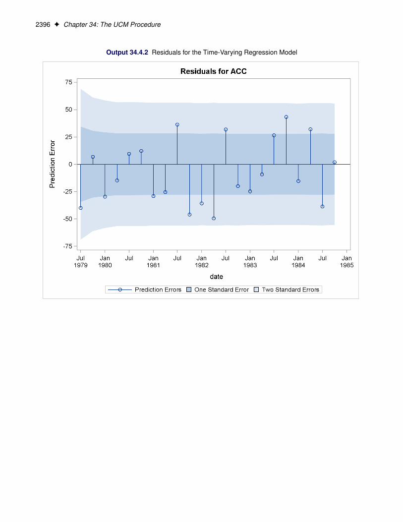
2396 F Chapter 34: The UCM Procedure
Output 34.4.2 Residuals for the Time-Varying Regression Model
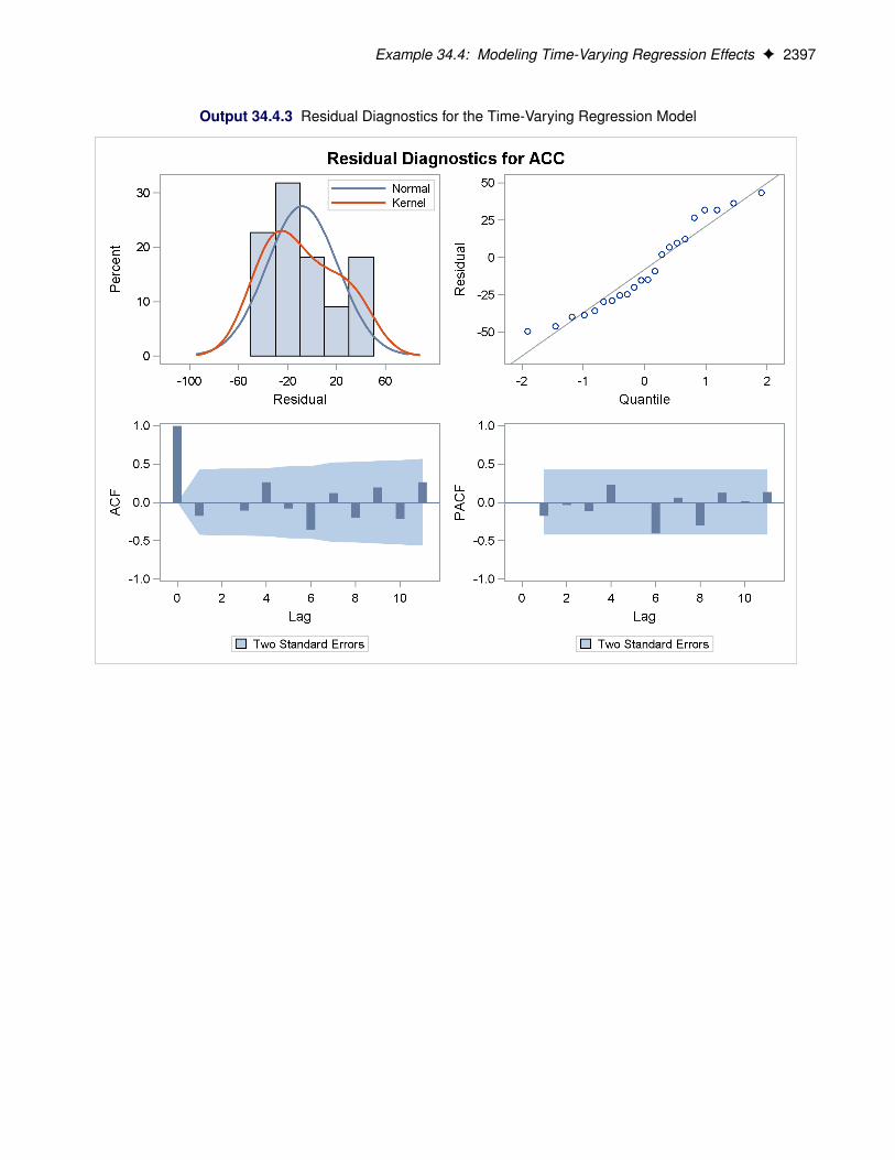
Example 34.4: Modeling Time-Varying Regression Effects F 2397
Output 34.4.3 Residual Diagnostics for the Time-Varying Regression Model
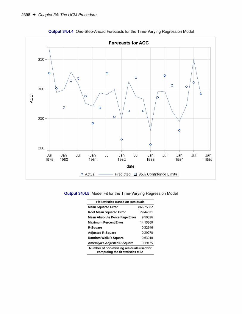
2398 F Chapter 34: The UCM Procedure
Output 34.4.4 One-Step-Ahead Forecasts for the Time-Varying Regression Model
Output 34.4.5 Model Fit for the Time-Varying Regression Model
Fit Statistics Based on Residuals
Mean Squared Error 866.75562
Root Mean Squared Error 29.44071
Mean Absolute Percentage Error 9.50326
Maximum Percent Error 14.15368
R-Square 0.32646
Adjusted R-Square 0.29278
Random Walk R-Square 0.63010
Amemiya's Adjusted R-Square 0.19175
Number of non-missing residuals used forcomputing the fit statistics = 22

Example 34.5: Trend Removal Using the Hodrick-Prescott Filter F 2399
Output 34.4.6 Parameter Estimates for the Time-Varying Regression Model
Final Estimates of the Free Parameters
Component Parameter EstimateApprox
Std Error t ValueApproxPr > |t|
Irregular Error Variance 480.92258 109.21980 4.40 <.0001
FUEL Coefficient 6.23279 0.67533 9.23 <.0001
batProgram Error Variance 84.22334 79.88166 1.05 0.2917
Example 34.5: Trend Removal Using the Hodrick-Prescott FilterHodrick-Prescott filter (Hodrick and Prescott 1997) is a popular tool in macroeconomics for fitting smoothtrend to time series. It is well known that the trend computation according to this filter is equivalent to fittingthe local linear trend plus irregular model with the level disturbance variance restricted to zero and the slopedisturbance variance restricted to be a suitable multiple of the irregular component variance. The multipleused depends on the frequency of the series; for example, for quarterly series the commonly recommendedmultiple is 1=1600 D 0:000625. For other intervals there is no consensus, but a frequently suggestedvalue for monthly series is 1=14400 and the value for an annual series can range from 1=400 D 0:0025
to 1=7 D 0:15. The data set considered in this example consists of quarterly GNP values for the UnitedStates from 1960 to 1991. In the UCM procedure statements that follow, the presence of the PROFILEoption in the ESTIMATE statement implies that the restriction that the disturbance variance of the slopecomponent be fixed at 0.000625 is interpreted differently: it implies that the disturbance variance of the slopecomponent be restricted to be 0.000625 times the estimated irregular component variance, as needed for theHodrick-Prescott filter. The plot of the fitted trend is shown in Output 34.5.1, and the plot of the smoothedirregular component, which corresponds to the detrended series, is given in Output 34.5.2. The detrendedseries can be further analyzed for business cycles.
proc ucm data=sashelp.gnp;id date interval=qtr;model gnp;irregular plot=smooth;level var=0 noest plot=smooth;slope var=0.000625 noest;estimate PROFILE;forecast plot=(decomp);
run;
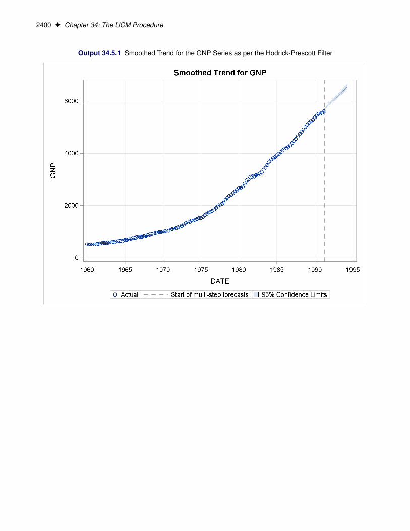
2400 F Chapter 34: The UCM Procedure
Output 34.5.1 Smoothed Trend for the GNP Series as per the Hodrick-Prescott Filter
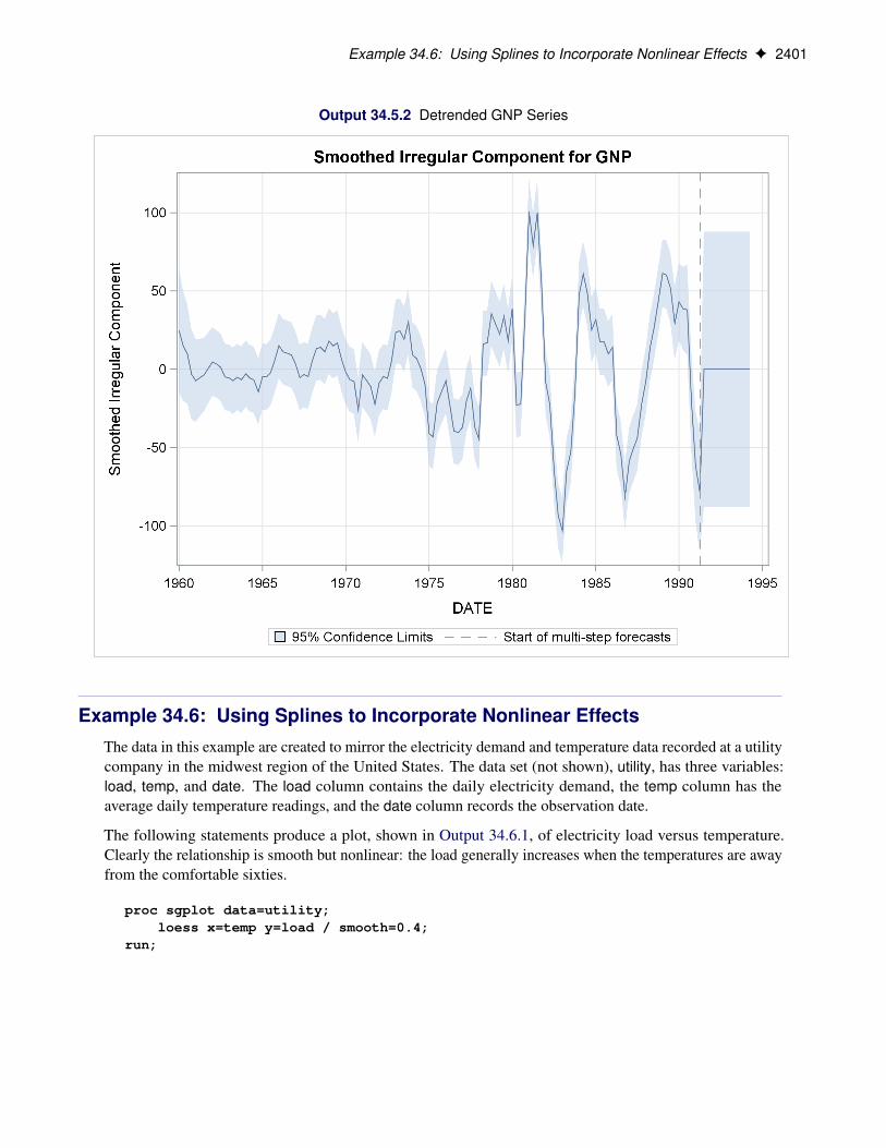
Example 34.6: Using Splines to Incorporate Nonlinear Effects F 2401
Output 34.5.2 Detrended GNP Series
Example 34.6: Using Splines to Incorporate Nonlinear EffectsThe data in this example are created to mirror the electricity demand and temperature data recorded at a utilitycompany in the midwest region of the United States. The data set (not shown), utility, has three variables:load, temp, and date. The load column contains the daily electricity demand, the temp column has theaverage daily temperature readings, and the date column records the observation date.
The following statements produce a plot, shown in Output 34.6.1, of electricity load versus temperature.Clearly the relationship is smooth but nonlinear: the load generally increases when the temperatures are awayfrom the comfortable sixties.
proc sgplot data=utility;loess x=temp y=load / smooth=0.4;
run;

2402 F Chapter 34: The UCM Procedure
Output 34.6.1 Load versus Temperature Plot
The time series plot of the load (not shown) also shows that, apart from a day-of-the-week seasonal effect,there are no additional easily identifiable patterns in the series. The series has no apparent upward ordownward trend. The following statements fit a UCM to the series that takes into account these observations.The particular choice of the model is a result of a little modeling exercise that compared a small number ofcompeting models. The chosen model is adequate but by no means the best possible. The temperature effectis modeled by a deterministic three-degree spline with knots at 30, 40, 50, 60, and 75. The knot locationsand the degree were chosen by visual inspection of the plot (Output 34.6.1). An autoreg component is usedin place of the simple irregular component, which improved the residual analysis. The last 60 days of dataare withheld for out-of-sample forecast evaluation (note the BACK= option in both the ESTIMATE andFORECAST statements). The OUTLIER statement is used to increase the number of outliers reported to 10.Since no CHECKBREAK option is used in the LEVEL statement, only the additive outliers are searched. Inthis example the use of the EXTRADIFFUSE= option in the ESTIMATE and FORECAST statements isuseful for discarding some early one-step-ahead forecasts and residuals with large variance.
proc ucm data=utility;id date interval=day;model load;autoreg;level plot=smooth;

Example 34.6: Using Splines to Incorporate Nonlinear Effects F 2403
splinereg temp knots=30 40 50 65 75 degree=3variance=0 noest;
season length=7 var=0 noest;estimate plot=panel back=60extradiffuse=50;
outlier maxnum=10;forecast back=60 lead=60
extradiffuse=50;run;
The parameter estimates are given in Output 34.6.2, and the residual goodness-of-fit statistics are shown inOutput 34.6.3. The residual diagnostic plots are shown in Output 34.6.4. The ACF and PACF plots appearsatisfactory, but the normality plots, particularly the Q-Q plot, show possible violations. It appears that, atleast in part, this nonNormal behavior of the residuals might be attributable to the outliers in the series. Theoutlier summary table, Output 34.6.5, shows the most likely outlying observations. Notice that most of theseoutliers are holidays, like July 4th, when the electricity load is lower than usual for that day of the week.
Output 34.6.2 Electricity Load: Parameter Estimates
The UCM ProcedureThe UCM Procedure
Final Estimates of the Free Parameters
Component Parameter EstimateApprox
Std Error t ValueApproxPr > |t|
Level Error Variance 0.21185 0.05025 4.22 <.0001
AutoReg Damping Factor 0.57522 0.03466 16.60 <.0001
AutoReg Error Variance 2.21057 0.20478 10.79 <.0001
temp Spline Coefficient_1 4.72502 1.93997 2.44 0.0149
temp Spline Coefficient_2 2.19116 1.71243 1.28 0.2007
temp Spline Coefficient_3 -7.14492 1.56805 -4.56 <.0001
temp Spline Coefficient_4 -11.39950 1.45098 -7.86 <.0001
temp Spline Coefficient_5 -16.38055 1.36977 -11.96 <.0001
temp Spline Coefficient_6 -18.76075 1.28898 -14.55 <.0001
temp Spline Coefficient_7 -8.04628 1.09017 -7.38 <.0001
temp Spline Coefficient_8 -2.30525 1.25102 -1.84 0.0654
Output 34.6.3 Electricity Load: goodness-of-fit
Fit Statistics Based on Residuals
Mean Squared Error 2.90945
Root Mean Squared Error 1.70571
Mean Absolute Percentage Error 2.92586
Maximum Percent Error 14.96281
R-Square 0.92739
Adjusted R-Square 0.92721
Random Walk R-Square 0.69618
Amemiya's Adjusted R-Square 0.92684
Number of non-missing residuals used forcomputing the fit statistics = 791
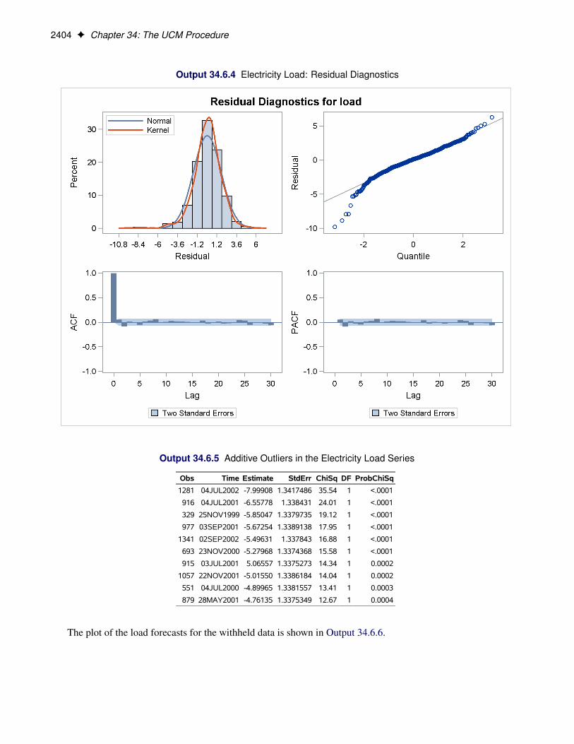
2404 F Chapter 34: The UCM Procedure
Output 34.6.4 Electricity Load: Residual Diagnostics
Output 34.6.5 Additive Outliers in the Electricity Load Series
Obs Time Estimate StdErr ChiSq DF ProbChiSq
1281 04JUL2002 -7.99908 1.3417486 35.54 1 <.0001
916 04JUL2001 -6.55778 1.338431 24.01 1 <.0001
329 25NOV1999 -5.85047 1.3379735 19.12 1 <.0001
977 03SEP2001 -5.67254 1.3389138 17.95 1 <.0001
1341 02SEP2002 -5.49631 1.337843 16.88 1 <.0001
693 23NOV2000 -5.27968 1.3374368 15.58 1 <.0001
915 03JUL2001 5.06557 1.3375273 14.34 1 0.0002
1057 22NOV2001 -5.01550 1.3386184 14.04 1 0.0002
551 04JUL2000 -4.89965 1.3381557 13.41 1 0.0003
879 28MAY2001 -4.76135 1.3375349 12.67 1 0.0004
The plot of the load forecasts for the withheld data is shown in Output 34.6.6.
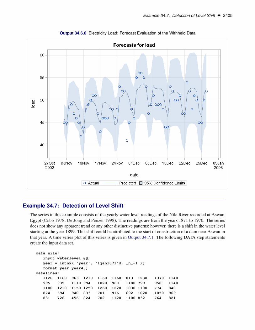
Example 34.7: Detection of Level Shift F 2405
Output 34.6.6 Electricity Load: Forecast Evaluation of the Withheld Data
Example 34.7: Detection of Level ShiftThe series in this example consists of the yearly water level readings of the Nile River recorded at Aswan,Egypt (Cobb 1978; De Jong and Penzer 1998). The readings are from the years 1871 to 1970. The seriesdoes not show any apparent trend or any other distinctive patterns; however, there is a shift in the water levelstarting at the year 1899. This shift could be attributed to the start of construction of a dam near Aswan inthat year. A time series plot of this series is given in Output 34.7.1. The following DATA step statementscreate the input data set.
data nile;input waterlevel @@;year = intnx( 'year', '1jan1871'd, _n_-1 );format year year4.;
datalines;1120 1160 963 1210 1160 1160 813 1230 1370 1140995 935 1110 994 1020 960 1180 799 958 11401100 1210 1150 1250 1260 1220 1030 1100 774 840874 694 940 833 701 916 692 1020 1050 969831 726 456 824 702 1120 1100 832 764 821

2406 F Chapter 34: The UCM Procedure
768 845 864 862 698 845 744 796 1040 759781 865 845 944 984 897 822 1010 771 676649 846 812 742 801 1040 860 874 848 890744 749 838 1050 918 986 797 923 975 8151020 906 901 1170 912 746 919 718 714 740
;
proc timeseries data=nile plot=series;id year interval=year;var waterlevel;
run;
Output 34.7.1 Nile Water Level
In this situation it is known that a shift in the water level occurred within the span of the series, and its effectcan be easily taken into account by including an appropriate indicator variable as a regressor. However, inmany situation such prior information is not available, and it is useful to detect such a shift in a data analyticfashion. You can check for breaks in the level by using the CHECKBREAK option in the LEVEL statement.The following statements fit a simple locally constant level plus error model to the series:
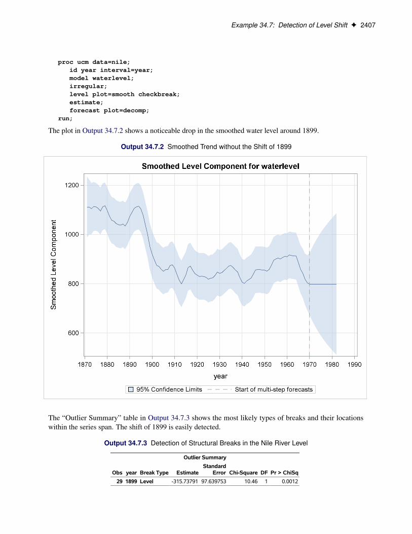
Example 34.7: Detection of Level Shift F 2407
proc ucm data=nile;id year interval=year;model waterlevel;irregular;level plot=smooth checkbreak;estimate;forecast plot=decomp;
run;
The plot in Output 34.7.2 shows a noticeable drop in the smoothed water level around 1899.
Output 34.7.2 Smoothed Trend without the Shift of 1899
The “Outlier Summary” table in Output 34.7.3 shows the most likely types of breaks and their locationswithin the series span. The shift of 1899 is easily detected.
Output 34.7.3 Detection of Structural Breaks in the Nile River Level
Outlier Summary
Obs year Break Type EstimateStandard
Error Chi-Square DF Pr > ChiSq
29 1899 Level -315.73791 97.639753 10.46 1 0.0012

2408 F Chapter 34: The UCM Procedure
The following statements specify a UCM that models the level of the river as a locally constant series with ashift in the year 1899, represented by a dummy regressor (SHIFT1899):
data nile;set nile;shift1899 = ( year >= '1jan1899'd );
run;
proc ucm data=nile;id year interval=year;model waterlevel = shift1899;irregular;level;estimate;forecast plot=decomp;
run;
The plot in Output 34.7.4 shows the smoothed trend, including the correction due to the shift in the year 1899.Notice the simplicity in the shape of the smoothed curve after the incorporation of the shift information.
Output 34.7.4 Smoothed Trend plus Shift of 1899
Example 34.8: ARIMA Modeling F 2409
Example 34.8: ARIMA ModelingThis example shows how you can use the UCM procedure for ARIMA modeling. The parameter estimatesand predictions for ARIMA models obtained by using PROC UCM will be close to those obtained by usingPROC ARIMA (in the presence of the ML option in its ESTIMATE statement) if the model is stationaryor if the model is nonstationary and there are no missing values in the data. See Chapter 7, “The ARIMAProcedure,” for additional details about the ARIMA procedure. However, if there are missing values inthe data and the model is nonstationary, then the UCM and ARIMA procedures can produce significantlydifferent parameter estimates and predictions. An article by Kohn and Ansley (1986) suggests a statisticallysound method of estimation, prediction, and interpolation for nonstationary ARIMA models with missingdata. This method is based on an algorithm that is equivalent to the Kalman filtering and smoothing algorithmused in the UCM procedure. The results of an illustrative example in their article are reproduced here usingthe UCM procedure. In this example an ARIMA(0,1,1)�(0,1,1)12 model is applied to the logarithm of the airseries in the sashelp.air data set. Four different missing value patterns are considered to highlight differentaspects of the problem:
• Data1. The full data set of 144 observations.
• Data2. The set of 78 observations that omit January through November in each of the last 6 years.
• Data3. The data set with the 5 observations July 1949, June, July, and August 1957, and July 1960missing.
• Data4. The data set with all July observations missing and June and August 1957 also missing.
The following DATA steps create these data sets:
data Data1;set sashelp.air;logair = log(air);
run;
data Data2;set data1;if year(date) >= 1955 and month(date) < 12 then logair = .;
run;
data Data3;set data1;if (year(date) = 1949 and month(date) = 7) then logair = .;if ( year(date) = 1957 and
(month(date) = 6 or month(date) = 7 or month(date) = 8))then logair = .;
if (year(date) = 1960 and month(date) = 7) then logair = .;run;
data Data4;set data1;if month(date) = 7 then logair = .;if year(date) = 1957 and (month(date) = 6 or month(date) = 8)
then logair = .;run;

2410 F Chapter 34: The UCM Procedure
The following statements specify the ARIMA.0; 1; 1/ � .0; 1; 1/12 model for the logair series in the first dataset (Data1):
proc ucm data=Data1;id date interval=month;model logair;irregular q=1 sq=1 s=12;deplag lags=(1)(12) phi=1 1 noest;estimate outest=est1;forecast outfor=for1;
run;
Note that the moving average part of the model is specified by using the Q=, SQ=, and S= options in theIRREGULAR statement and the differencing operator, .1�B/.1�B12/, is specified by using the DEPLAGstatement. The model does not contain an intercept term; therefore no LEVEL statement is needed. Theparameter estimates are saved in a data set EST1 by using the OUTEST= option in the ESTIMATE statementand the forecasts and the component estimates are saved in a data set FOR1 by using the OUTFOR= optionin the FORECAST statement. The same analysis is performed on the other three data sets, but is not shownhere.
Output 34.8.1 resembles Table 1 in Kohn and Ansley (1986). This table is generated by merging the parameterestimates from the four analyses. Only the moving average parameter estimates and their standard errors arereported. The columns EST1 and STD1 correspond to the estimates for Data1. The parameter estimates andtheir standard errors for other three data sets are similarly named. Note that the parameter estimates closelymatch the parameter estimates in the article. However, their standard errors differ slightly. This differencecould be the result of different ways of computing the Hessian at the optimum. The white noise error varianceestimates are not reported here, but they agree quite closely with those in the article.
Output 34.8.1 Data Sets 1–4: Parameter Estimates and Standard Errors
PARAMETER est1 std1 est2 std2 est3 std3 est4 std4
MA_1 0.402 0.090 0.457 0.121 0.408 0.092 0.431 0.091
SMA_1 0.557 0.073 0.758 0.236 0.566 0.075 0.573 0.074
Output 34.8.2 resembles Table 2 in Kohn and Ansley (1986). It contains forecasts and their standard errorsfor the four data sets. The numbers are very close to those in the article.
Output 34.8.2 Data Sets 1–4: Forecasts and Standard Errors
DATE for1 std1 for2 std2 for3 std3 for4 std4
JAN61 6.110 0.037 6.084 0.052 6.110 0.037 6.111 0.037
FEB61 6.054 0.043 6.091 0.058 6.054 0.043 6.055 0.043
MAR61 6.172 0.048 6.247 0.063 6.173 0.048 6.174 0.048
APR61 6.199 0.053 6.205 0.068 6.199 0.053 6.200 0.052
MAY61 6.233 0.057 6.199 0.072 6.232 0.058 6.233 0.056
JUN61 6.369 0.061 6.308 0.076 6.367 0.062 6.368 0.060
JUL61 6.507 0.065 6.409 0.079 6.497 0.067 . .
AUG61 6.503 0.069 6.414 0.082 6.503 0.069 6.503 0.067
SEP61 6.325 0.072 6.299 0.085 6.325 0.072 6.326 0.071
OCT61 6.209 0.075 6.174 0.087 6.209 0.076 6.209 0.074
NOV61 6.063 0.079 6.043 0.089 6.064 0.079 6.064 0.077
DEC61 6.168 0.082 6.174 0.086 6.168 0.082 6.169 0.080

Example 34.8: ARIMA Modeling F 2411
Output 34.8.3 is based on Data2. It resembles Table 3 in Kohn and Ansley (1986). The columns S_SERIESand VS_SERIES in the OUTFOR= data set contain the interpolated values of logair and their variances.The estimate column in Output 34.8.3 reports interpolated values (which are the same as S_SERIES),and the std column reports their standard errors (which are computed as square root of VS_SERIES) forJanuary–November 1957. The actual logair values for these months, which are missing in Data2, are alsoprovided for comparison. The numbers are very close to those in the article.
Output 34.8.3 Data Set 2: Interpolated Values and Standard Errors
DATE logair estimate std
JAN57 5.753 5.733 0.045
FEB57 5.707 5.738 0.049
MAR57 5.875 5.893 0.052
APR57 5.852 5.850 0.054
MAY57 5.872 5.843 0.055
JUN57 6.045 5.951 0.055
JUL57 6.142 6.051 0.055
AUG57 6.146 6.055 0.054
SEP57 6.001 5.938 0.052
OCT57 5.849 5.812 0.049
NOV57 5.720 5.680 0.045
Output 34.8.4 resembles Table 4 in Kohn and Ansley (1986). These numbers are based on Data3, and theyalso are very close to those in the article.
Output 34.8.4 Data Set 3: Interpolated Values and Standard Errors
DATE logair estimate std
JUL49 4.997 5.013 0.031
JUN57 6.045 6.024 0.030
JUL57 6.142 6.147 0.031
AUG57 6.146 6.148 0.030
JUL60 6.433 6.409 0.031
Output 34.8.5 resembles Table 5 in Kohn and Ansley (1986). As before, the numbers are very close to thosein the article.
Output 34.8.5 Data Set 4: Interpolated Values and Standard Errors
DATE logair estimate std
JUN57 6.045 6.023 0.030
AUG57 6.146 6.147 0.030
The similarity between the outputs in this example and the results shown in Kohn and Ansley (1986)demonstrate that PROC UCM can be effectively used for nonstationary ARIMA models with missing data.

2412 F Chapter 34: The UCM Procedure
References
Akaike, H. (1974), “A New Look at the Statistical Model Identification,” IEEE Transactions on AutomaticControl, AC-19, 716–723.
Anderson, T. W. (1971), The Statistical Analysis of Time Series, New York: John Wiley & Sons.
Bloomfield, P. (2000), Fourier Analysis of Time Series, 2nd Edition, New York: John Wiley & Sons.
Box, G. E. P. and Jenkins, G. M. (1976), Time Series Analysis: Forecasting and Control, Rev. Edition, SanFrancisco: Holden-Day.
Bozdogan, H. (1987), “Model Selection and Akaike’s Information Criterion (AIC): The General Theory andIts Analytical Extensions,” Psychometrika, 52, 345–370.
Brockwell, P. J. and Davis, R. A. (1991), Time Series: Theory and Methods, 2nd Edition, New York:Springer-Verlag.
Burnham, K. P. and Anderson, D. R. (1998), Model Selection and Inference: A Practical Information-Theoretic Approach, New York: Springer-Verlag.
Cobb, G. W. (1978), “The Problem of the Nile: Conditional Solution to a Change Point Problem,” Biometrika,65, 243–251.
De Jong, P. and Chu-Chun-Lin, S. (2003), “Smoothing with an Unknown Initial Condition,” Journal of TimeSeries Analysis, 24, 141–148.
De Jong, P. and Penzer, J. (1998), “Diagnosing Shocks in Time Series,” Journal of the American StatisticalAssociation, 93, 796–806.
Durbin, J. and Koopman, S. J. (2001), Time Series Analysis by State Space Methods, Oxford: OxfordUniversity Press.
Hannan, E. J. and Quinn, B. G. (1979), “The Determination of the Order of an Autoregression,” Journal ofthe Royal Statistical Society, Series B, 41, 190–195.
Harvey, A. C. (1989), Forecasting, Structural Time Series Models, and the Kalman Filter, Cambridge:Cambridge University Press.
Harvey, A. C. (2001), “Testing in Unobserved Components Models,” Journal of Forecasting, 20, 1–19.
Hodrick, R. J. and Prescott, E. C. (1997), “Postwar U.S. Business Cycles: An Empirical Investigation,”Journal of Money, Credit, and Banking, 29, 1–16.
Hurvich, C. M. and Tsai, C.-L. (1989), “Regression and Time Series Model Selection in Small Samples,”Biometrika, 76, 297–307.
Jones, R. H. (1980), “Maximum Likelihood Fitting of ARMA Models to Time Series with Missing Observa-tions,” Technometrics, 22, 389–396.
Kohn, R. and Ansley, C. F. (1986), “Estimation, Prediction, and Interpolation for ARIMA Models withMissing Data,” Journal of the American Statistical Association, 81, 751–761.

References F 2413
Rodriguez, A. and Ruiz, E. (2010), “Bootstrap Prediction Mean Squared Errors of Unobserved StatesBased on the Kalman Filter with the Estimated Parameters,” Working Paper 10-03 (01), Statistics andEconometric Series, Departamento de Estadística, Universidad Carlos de Madrid.
Schwarz, G. (1978), “Estimating the Dimension of a Model,” Annals of Statistics, 6, 461–464.
West, M. and Harrison, J. (1999), Bayesian Forecasting and Dynamic Models, 2nd Edition, New York:Springer-Verlag.
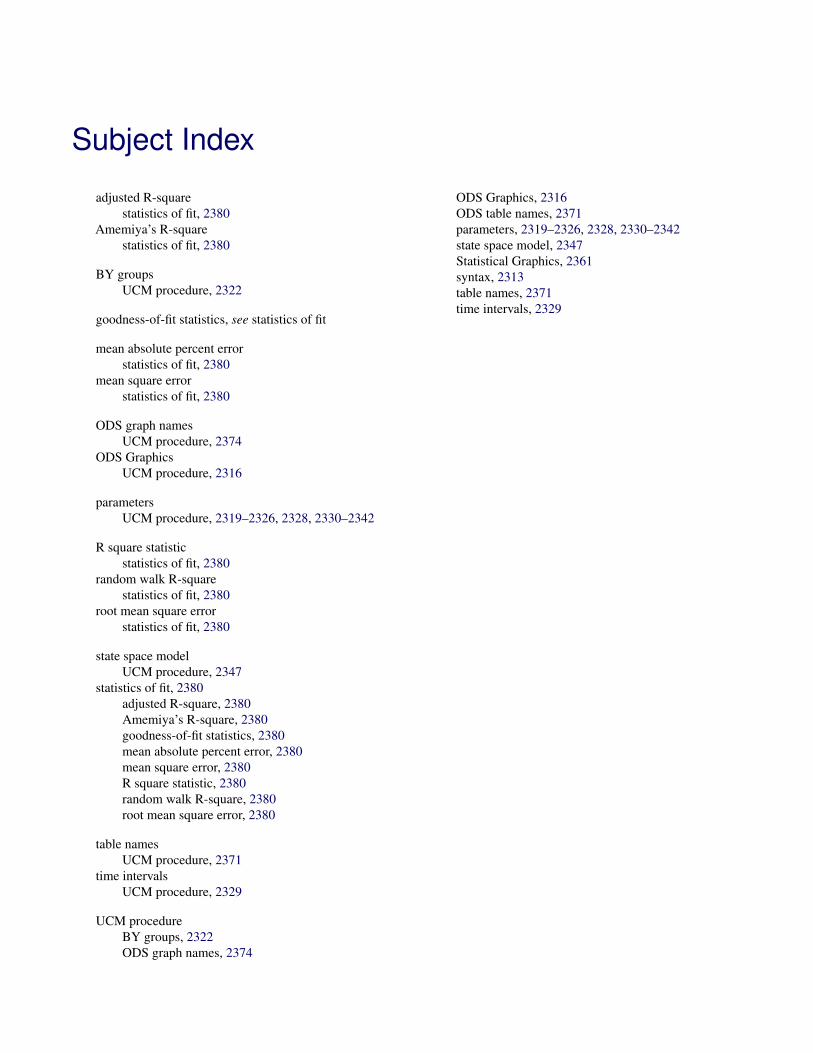
Subject Index
adjusted R-squarestatistics of fit, 2380
Amemiya’s R-squarestatistics of fit, 2380
BY groupsUCM procedure, 2322
goodness-of-fit statistics, see statistics of fit
mean absolute percent errorstatistics of fit, 2380
mean square errorstatistics of fit, 2380
ODS graph namesUCM procedure, 2374
ODS GraphicsUCM procedure, 2316
parametersUCM procedure, 2319–2326, 2328, 2330–2342
R square statisticstatistics of fit, 2380
random walk R-squarestatistics of fit, 2380
root mean square errorstatistics of fit, 2380
state space modelUCM procedure, 2347
statistics of fit, 2380adjusted R-square, 2380Amemiya’s R-square, 2380goodness-of-fit statistics, 2380mean absolute percent error, 2380mean square error, 2380R square statistic, 2380random walk R-square, 2380root mean square error, 2380
table namesUCM procedure, 2371
time intervalsUCM procedure, 2329
UCM procedureBY groups, 2322ODS graph names, 2374
ODS Graphics, 2316ODS table names, 2371parameters, 2319–2326, 2328, 2330–2342state space model, 2347Statistical Graphics, 2361syntax, 2313table names, 2371time intervals, 2329

Syntax Index
ALIGN= optionID statement (UCM), 2329
ALPHA= optionFORECAST statement (UCM), 2327
ALPHA=optionOUTLIER statement (UCM), 2334
AR optionIRREGULAR statement (UCM), 2331
AUTOREG statementUCM procedure, 2319
BACK= optionESTIMATE statement (UCM), 2325FORECAST statement (UCM), 2327
BLOCKSEASON statementUCM procedure, 2320
BLOCKSIZE= optionBLOCKSEASON statement (UCM), 2321
BOOTSTRAP= optionFORECAST statement (UCM), 2327
BY statementUCM procedure, 2322
CHECKBREAK optionLEVEL statement (UCM), 2333
CYCLE statementUCM procedure, 2322
DATA= optionPROC UCM statement, 2316
DEGREE= optionSPLINEREG statement (UCM), 2340SPLINESEASON statement (UCM), 2341
DEPLAG statementUCM procedure, 2323
DROPH= optionSEASON statement (UCM), 2337
ESTIMATE statementUCM procedure, 2324
EXTRADIFFUSE= optionESTIMATE statement (UCM), 2325FORECAST statement (UCM), 2328
FORECAST statementUCM procedure, 2327
ID statementUCM procedure, 2329
INTERVAL= optionID statement (UCM), 2329
IRREGULAR statementUCM procedure, 2329
KEEPH= optionSEASON statement (UCM), 2337
KNOTS= optionSPLINEREG statement (UCM), 2340SPLINESEASON statement (UCM), 2341
LAGS= optionDEPLAG statement (UCM), 2324
LEAD= optionFORECAST statement (UCM), 2328
LENGTH= optionSEASON statement (UCM), 2338SPLINESEASON statement (UCM), 2341
LEVEL statementUCM procedure, 2332
MAXNUM= optionOUTLIER statement (UCM), 2334
MAXPCT= optionOUTLIER statement (UCM), 2335
MODEL statementUCM procedure, 2334
NBLOCKS= optionBLOCKSEASON statement (UCM), 2321
NKNOTS= optionSPLINEREG statement (UCM), 2340
NLOPTIONS statementUCM procedure, 2334
NOEST optionAUTOREG statement (UCM), 2319BLOCKSEASON statement (UCM), 2321CYCLE statement (UCM), 2323DEPLAG statement (UCM), 2324IRREGULAR statement (UCM), 2330, 2332LEVEL statement (UCM), 2333RANDOMREG statement (UCM), 2336SEASON statement (UCM), 2338SLOPE statement (UCM), 2339SPLINEREG statement (UCM), 2340SPLINESEASON statement (UCM), 2341
NOPRINT optionPROC UCM statement, 2316
NOPROFILE
ESTIMATE statement (UCM), 2325
OFFSET= optionBLOCKSEASON statement (UCM), 2321SPLINESEASON statement (UCM), 2341
OUTEST= optionESTIMATE statement (UCM), 2325
OUTFOR= optionFORECAST statement (UCM), 2328
OUTLIER statementUCM procedure, 2334
P optionIRREGULAR statement (UCM), 2332
PERFORMANCE statementUCM procedure, 2335
PERIOD= optionCYCLE statement (UCM), 2323
PHI= optionDEPLAG statement (UCM), 2324
PLOT optionAUTOREG statement (UCM), 2320BLOCKSEASON statement (UCM), 2321CYCLE statement (UCM), 2323ESTIMATE statement (UCM), 2325FORECAST statement (UCM), 2328IRREGULAR statement (UCM), 2330PROC UCM statement, 2316RANDOMREG statement (UCM), 2336SEASON statement (UCM), 2338SLOPE statement (UCM), 2339SPLINEREG statement (UCM), 2340SPLINESEASON statement (UCM), 2341
PLOTS optionPROC UCM statement, 2316
PRINT optionAUTOREG statement (UCM), 2320BLOCKSEASON statement (UCM), 2321CYCLE statement (UCM), 2323ESTIMATE statement (UCM), 2326FORECAST statement (UCM), 2328IRREGULAR statement (UCM), 2330LEVEL statement (UCM), 2333OUTLIER statement (UCM), 2335RANDOMREG statement (UCM), 2336SEASON statement (UCM), 2338SLOPE statement (UCM), 2339SPLINESEASON statement (UCM), 2341
PRINTALL optionPROC UCM statement, 2319
PROC UCM statement, 2316, see UCM procedurePROFILE
ESTIMATE statement (UCM), 2326
Q option
IRREGULAR statement (UCM), 2332
RANDOMREGUCM procedure, 2335
RHO= optionAUTOREG statement (UCM), 2320CYCLE statement (UCM), 2323
RKNOTS optionSPLINESEASON statement (UCM), 2342
S optionIRREGULAR statement (UCM), 2332
SAR optionIRREGULAR statement (UCM), 2332
SEASON statementUCM procedure, 2336
SKIPFIRST= optionESTIMATE statement (UCM), 2327FORECAST statement (UCM), 2329
SKIPLAST= optionESTIMATE statement (UCM), 2325
SLOPE statementUCM procedure, 2338
SMA optionIRREGULAR statement (UCM), 2332
SP optionIRREGULAR statement (UCM), 2332
SPLINEREGUCM procedure, 2339
SPLINESEASONUCM procedure, 2341
SQ optionIRREGULAR statement (UCM), 2332
TYPE=optionBLOCKSEASON statement (UCM), 2322SEASON statement (UCM), 2338
UCM procedure, 2313syntax, 2313
UCM procedure, PROC UCM statementPLOT option, 2316
VARIANCE= optionAUTOREG statement (UCM), 2320CYCLE statement (UCM), 2323IRREGULAR statement (UCM), 2330LEVEL statement (UCM), 2333RANDOMREG statement (UCM), 2336SLOPE statement (UCM), 2339SPLINEREG statement (UCM), 2340SPLINESEASON statement (UCM), 2342
VARIANCE=optionBLOCKSEASON statement (UCM), 2322SEASON statement (UCM), 2338