The two-level atom Milne-Eddington model curve of … · 8. Line formation The two-level atom...

8. Line formation

The two-level atom

Milne-Eddington model

curve of growth

Two-level approximation

We consider schematic line-formation cases with easy solution

highly simplified: not accurate, but provide insight into the mechanisms at work in real stellar atmospheres.

Consider an atomic model with only two important levels: lower l and upper u.

Although highly simplified, it well approximates the situation for some lines, e.g. resonance lines from the ground state.


niXj 6=i(Rij + C ij) + ni(Rik + Cik) =

Xj 6=i

nj(Rji+ Cji) + np(Rki+ Cki)

Rate equations (statistical equilibrium)

Consider two levels u and l: isolating the transitions between them

nl(Rlu+ Clu) = nu(Rul + Cul)

and neglecting all transitions involving j

l,u, plus recombinations/ionizations:

nl(Rlu+Clu) + nlXj 6=l,u

(Rlj+Clj)+nl(Rlk+Clk) = nu(Rul+Cul) +Xj 6=l,u

nj(Rjl+Cjl)+np(Rkl+Ckl)


nl(Blu

∞Z0

ϕνJνdν+ C lu) = nu (Aul +Bul

∞Z0

ϕνJνdν +Cul)

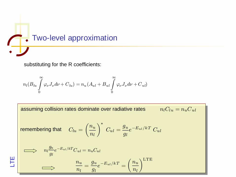
substituting for the R coefficients:

assuming collision rates dominate over radiative rates nlClu = nuCul

remembering that

nlgu

gle−Eul/kTCul = nuCul

nunl=gugle−Eul/kT =

µnunl

¶LTE

Clu =

µnunl

¶∗Cul =

gugle−Eul/kT Cul

LTE

LTE


Calculation of the line source function

κlineν = (nlBlu − nuBul) ϕν hν4π

²lineν = nuAul ϕνhν

4π

S lineν =²lineν

κlineν

=nuAul

nlBlu− nuBul =Aul

nlnuBlu −Bul

with Blu =guglBul Aul =

2hν3

c2Bul

S lineν =2hν3

c21

nlgunugl

− 1

Note: this is the general expressionfor the line source function in NLTE. It is always valid (not only in 2-level approximation). What is different in the general case, is how nl , nu are computed


If we substitute

we recover the Planck function

E = hν

S lineν =2hν3

c21

ehν/kT − 1 = Bν(T )

For the 2-level atom we found nl(Blu

∞Z0

ϕνJνdν+ C lu) = nu (Aul +Bul

∞Z0

ϕνJνdν +Cul)

and substituting in S

:

nunl=gugle−Eul/kT =

µnunl

¶∗

LTE

LTE


S lineν =2hν3

c2

c2

2hν3

Rϕν 0Jν0dν 0 + e−hν/kT Cul/Aul1 + Cul

Aul(1− e−hν/kT ) =

=1

1 + CulAul(1− e−hν/kT )

Zϕν 0Jν 0dν

0 +2hν3

c2e−hν/kTCul/Aul

1 + CulAul(1− e−hν/kT )

2hν3

c21

ehν/kT − 1(1− e−hν/kT )Cul/Aul1 + Cul

Aul(1 − e−hν/kT )

:=

1 –

B

(T)


² :=(1− e−hν/kT ) Cul/Aul1 + Cul


²0

1 + ²0

Slineν = (1− ²)∞Z0

ϕν 0Jν0dν0 + ² Bν(T ) =

∞R0

ϕν0Jν0 dν0 + ²0 Bν(T )

1 + ²0

scattering term thermal term

Comparison with Chapter 3: Continuum source function withtrue absorption + scattering

line source function has similar termsexcept that we also allow fornon-coherent scattering

Sν =κν

κν + σνBν +

σν

κν + σνJν

photons are either destroyed into thermal pool or scattered without change in frequency and isotropically

photons are created in thermal processes (

B

)destruction probability


a) Cul ÀAul

= 1

S

= B

(T) LTE

b) Cul ¿ Aul

≈

0

S

= ∫

0

J0

d0

extreme non-LTE

Chapter 3: S

= J

for pure coherent scatteringnow S

= ∫

0

J0

d0

non-coherent scattering

deep layers: collisions dominate 0

À1 or

= 1 thermal term dominanthigher layers: collisions non-important 0

≈

0

= 0 scattering term dominant

² :=(1− e−hν/kT ) Cul/Aul1 + Cul


²0

1 + ²0

Slineν = (1− ²)∞Z0

ϕν 0Jν0dν0 + ² Bν(T ) =

∞R0

ϕν0Jν0 dν0 + ²0 Bν(T )

1 + ²0


microscopically there is a photon absorption l u followed by re-emission

2-level atom is a special NLTE case

in general the coupling between J

, ni and S

is far more complicated

²lineν = κlineν Jνas in a coherent scattering process (e.g. Thomson scattering)complete redistribution: emission and absorption profiles identical

This second case (S

B

) has a macroscopic interpretation in terms of scattering

Slineν =² lineν

κlineν

=

∞Z0

ϕν 0Jν 0dν0 =⇒ ²lineν = κlineν

∞Z0

ϕν 0Jν0dν0

for a narrow absorption profile function ϕν 0 ≈ δ(ν0 − ν)


Moving outward in the photosphere scattering term dominates

At some point we reach the region where photons are being lost from the star (small optical depth) J

decreases with height S

decreases with height

absorption line

mapping between source function (decreasing outward) and line profile

line absorption coefficient larger at line center see higher layers

wings formed in deeper layers than line core

adapted from Gray, 92

The Milne-Eddington model

We have defined line and continuum coefficients for absorption and emission

Total absorption coefficient is

with

from scattering in the continuum

The total optical depth is(larger than in the continuum!)

Qualitative line formation

Barbier-Eddington relation: I(0,) ≈

S(=)In LTE: S

= B

(T)

T decreases outward S

decreases outward absorption line

κν = κCν + κL

ν + σ


Transfer equation:

μdIν(μ)

dx= (κC

ν + κLν + σ)Iν − ²Cν − ²Lν − σJν

Without dealing with the general case for the computation of all coefficients we assume:

- LTE in the continuum

- scattering negligible in the continuum

- 2-level atom in the line

²CνκCν

= Bν(T)

σ ¿ κCν


μdIνdx

= (κC

ν + κL

ν)

·Iν −

κCν

κCν + κL

ν

Bν −κLν

κCν + κLν

SLν

¸

with βν =κLν

κCν

dτν = (κC

ν + κL

ν)dx = κC

ν (1 + βν)dx

λν =1+ ²βν1 + βν

S lineν = (1− ²)∞Z0

ϕν 0Jν 0dν0 + ² Bν(T)with

from

μdIνdτν

= Iν − λνBν − (1− λν)

∞Z0

ϕνJνdν


assumptions (for analytical solution)1

,

and

constant with depth2. B

linear in continuum optical depth

3. ∞Z0

ϕνJνdν ≈ Jν

plus the Eddington approximation Kν =1

2

1Z−1Iνμ

2dμ =1

3Jν

Hν(0) =1√3Jν(0)

Bν = a+ b τc

dτc =dτν1 + βν

τc =τν

1 + βν

boundary condition (without proof)

λν =1+ ²βν1 + βν


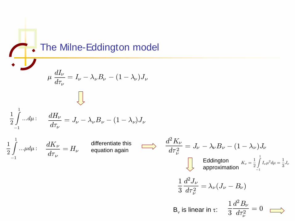
μdIνdτν

= Iν − λνBν − (1− λν)Jν

1

2

1Z−1...dμ : dHν

dτν= Jν − λνBν − (1− λν)Jν

1

2

1Z−1...μdμ :

dKν

dτν=Hν

d2Kν

dτ 2ν= Jν − λνBν − (1− λν)Jν

1

3

d2Jνdτ 2ν

= λν(Jν −Bν)

B

is linear in : 1

3

d2Bν

dτ2ν= 0

differentiate thisequation again

Eddingtonapproximation


1

3

d2

dτ2ν(Jν −Bν) = λν(Jν −Bν)

solution: Jν −Bν = αν e−√3λν τν + γν e

√3λν τν

boundary conditions τν →∞ : Jν → Bν → γν = 0

τν = 0 : Hν(0) =1√3Jν(0) we use this boundary condition

to determine on the next 2 pages


from dKν

dτν=1

3

dJνdτν

= Hν

1

3

dJνdτν

¯̄̄̄τν=0

=Hν(0) =1√3Jν(0)

from

and

Jν −Bν = αν e−√3λν τν + γν e

√3λν τν

Bν = a+ b τc

Jν(0) = αν +Bν(0) = αν + a =1√3

dJνdτν

¯̄̄̄τν=0

1√3

dJνdτν

¯̄̄̄τν=0

=1√3[−αν

p3λν +

b

1 + βν] = αν + a

dBν

dτν=dBν

dτc

1

1 + βν


define pν =b

1 + βν

αν =b

1+βν−√3a

(√3 +

√3λν)

thermalization depth: for

J

B

Jν(τ) = a + pντν +pν − a

√3√

3 +√3λν

e−√3λν τν

Hν(0) =1√3Jν(0) =

a√3+

pν − a√3

3(1 +√λν)

=1

3

pν + a√3λν

1 +√λν

τν ≥ 1√λν

J

< B

in outer parts of atmosphere

Bν = a+ b τc

dτc =dτν1 + βν

τc =τν

1 + βν

Bν

λν =1+ ²βν1 + βν

βν =κLν

κCν

dτν = (κC

ν + κL

ν)dx = κC

ν (1 + βν)dx


residual flux Rν =Hν(0)

Hc(0)

for Hc :

Hc(0) =1

3

b + a√3

2

βν =κLν

κCν

= 0 =⇒ pν = b λν = 1

Rν =Hν(0)

Hc(0)= 2

pν +√3λνa

(1 +√λν)(b +

√3a)

compute the line profile


a) case

= 1 (LTE: pure absorption lines)

SLν =Bν

Scν = Bν

Rν =b

1+βν+√3a

b+√3a

for strong line:

= L / c À 1 Rν =

√3a

b +√3a=

Bν(0)

Bν(τc = 1/√3)6= 0

λν =1+ ²βν1 + βν

= 1

emergent flux determined by surface value of Planck function

isothermal atmosphere (B

= a)

Zwaan, 93, Lecture notes

Bν = a+ b τc

dτc =dτν1 + βν

τc =τν

1 + βν


in LTE the residual flux is non-zero also for strong absorption lines

e.g. in the Sun b/a ≈

9/4

R = 0.44 (

= 5000 A)

However resonance lines such as Na D have R ∼

10-3 – 10-4

b) case

= 0 (extreme non-LTE: pure scattering lines)

Rν =

11+βν

+q

31+βν

a

(1 +q

11+βν

)(b +√3a)

as

∞ (strong line): R

= 0

λν =1

1+ βν

for a strong line formed by scattering

scattering removes all photons no photon emerges from surface

λν =1+ ²βν1 + βν

βν =κLν

κCν

dτν = (κC

ν + κL

ν)dx = κC

ν (1 + βν)dx

Theoretical curve of growth

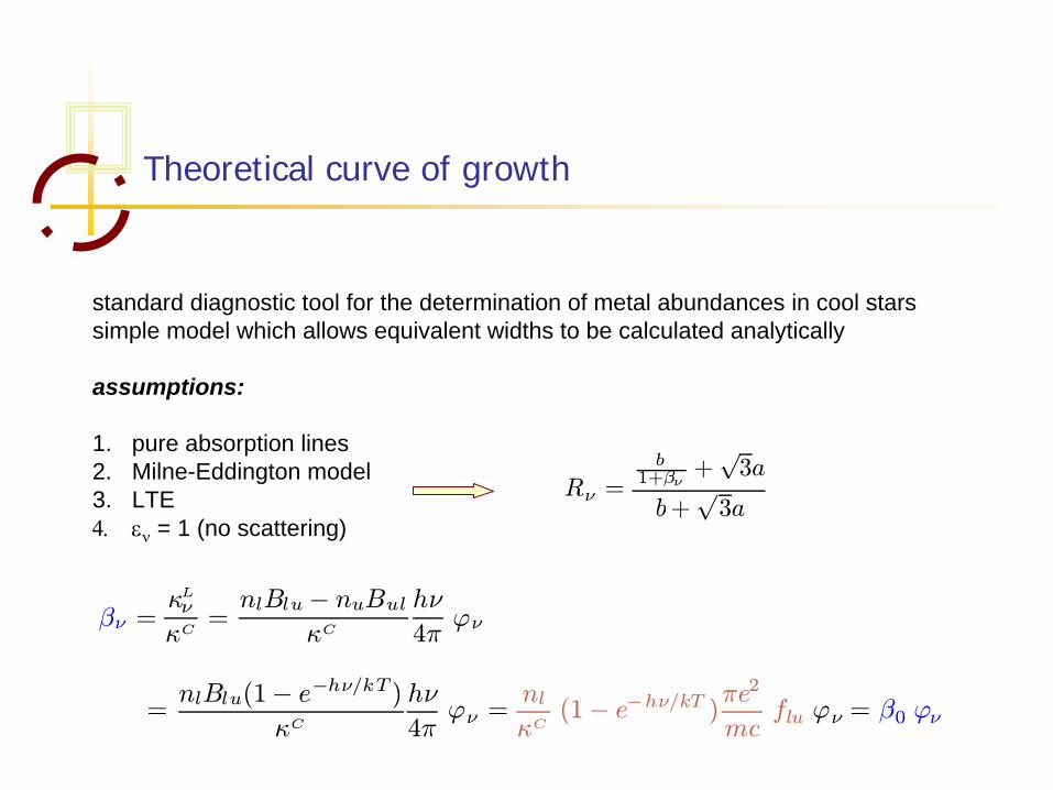
standard diagnostic tool for the determination of metal abundances in cool starssimple model which allows equivalent widths to be calculated analytically

assumptions:

1. pure absorption lines2. Milne-Eddington model3. LTE

= 1 (no scattering)

Rν =b

1+βν+√3a

b+√3a

βν =κLνκC

=nlBlu− nuBul

κC

hν

4πϕν

=nlBlu(1− e−hν/kT )

κC

hν

4πϕν =

nlκC

(1− e−hν/kT )πe2

mcflu ϕν = β0 ϕν


Rν =b

1+β0 ϕν+√3a

b+√3a

Aν = 1 −Rν =β0 ϕν

1 + β0 ϕν

µb

b +√3a

¶=A0

β0 ϕν

1 + β0 ϕνline depth

0 increasein LTE non-zero central intensity even for strong lines (

∞)


Equivalent width Wν =

∞Z0

Aν dν

Wν =A0β0

∞Z0

ϕν

1 + β0 ϕν

dν

use Voigt profile ϕ(ν − ν0) =1

π 1/2 ∆νDH(a, v)

≈ e−v2 + aπ1/2v2


3 regimes

1. linear ~ 0

2. saturation ~ (ln 0)0.5

log 0

log W

1. linear regime:

unsaturated Doppler core H(a, v) ≈ e−v2

3. damping ~ 00.5

β0∆νD

< 1

Wν ≈ A0β0√π

∞Z−∞

e−v2

1 + β0√π∆νD

dv =A0β0√

π

∞Z−∞

e−v2

µ1− β0√

π∆νDe−v

2

+ ...

¶dv ≈ A0β0


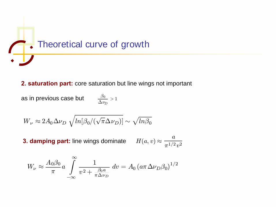
2. saturation part:

core saturation but line wings not important

as in previous case but β0∆νD

> 1

Wν ≈ 2A0∆νDqln[β0/(

√π∆νD)]∼

plnβ0

3. damping part:

line wings dominate H(a, v)≈ a

π1/2v2

Wν ≈ A0β0πa

∞Z−∞

1

v2+ β0aπ∆νD

dv = A0 (aπ∆νDβ0)1/2


effect on a spectral line of the increase of absorbers along the line of sight


In general: Wν = f(β0) or f

µβ0

∆νD√π

¶= f(β∗)

β ∗ =πe2

mcflunlκC

(1− e−hν/kT ) 1

∆νD√π

κcν = κc0(1− e−hν/kT )

nl = n1gl

g1(1− e−hν/kT )

in LTE

Boltzmann

∆νD =ν0c

r2kT

m=1

λ

r2kT

m


log β∗ = log(glfluλ) + loge−E1l/kT + log

µn1g1κc0

√πe2

mc

rm

2kT

¶

log β∗ = log(glfluλ)− 5040E1lT+ logC

1. for a single ionization stage C = const2. lines belonging to one ionization stage should form a curve of growth: * varies as a

function of line transition 3. if T and 0 known: shift observed W

curve until it matches theoretical curve4. from n1 calculate total abundances using Saha-Boltzmann equations


empirical curve of growth

plot log (W/) vs log (gf) - 5040 E1l /T for each line

adjust T to minimize scatter around a mean curve (excitation temperature typical of line formation region)

empirical curve of growth foriron and titanium lines in the Sun

log(glfluλ) − 5040E1lT+ logC

Mihalas, 78

The two-level atom Milne-Eddington model curve of … · 8. Line formation The two-level atom...

Documents

Transcript of The two-level atom Milne-Eddington model curve of … · 8. Line formation The two-level atom...