The Tunneling Algorithm for Partial CSPs and …The Tunneling Algorithm for Partial CSPs and...

The Tunneling Algorithm for Partial CSPs andCombinatorial Optimization Problems

Chris Voudouris [email protected]

Edward Tsang [email protected]

Department of Computer Science,University of Essex,Colchester, C04 3SQ, UK

Abstract

Constraint satisfaction is the core of a large number of problems, notably scheduling.Because of their potential for containing the combinatorial explosion problem in constraintsatisfaction, local search methods have received a lot of attention in the last few years. Theproblem with these methods is that they can be trapped in local minima. GENET is aconnectionist approach to constraint satisfaction. It escapes local minima by means of aweight adjustment scheme, which has been demonstrated to be highly effective. Thetunneling algorithm described in this paper is an extension of GENET for optimization. Themain idea is to introduce modifications to the function which is to be optimized by thenetwork (this function mirrors the objective function which is specified in the problem). Wedemonstrate the outstanding performance of this algorithm on constraint satisfactionproblems, constraint satisfaction optimization problems, partial constraint satisfactionproblems, radio frequency allocation problems and traveling salesman problems.

1. Introduction

Local search methods being general approximation algorithms have been used widely to solveoptimization problems. A recent application domain of local search is the ConstraintSatisfaction Problem (CSP) (Tsang, 1993). A CSP involves assigning values to a set ofvariables satisfying a set of constraints. One of the best known work in applying local search toconstraint satisfaction is the heuristic repair method which uses the min-conflicts heuristic(Minton et. al. 1992). A min-conflict based move (also mentioned as repair or "flip") is realizedby re-assigning to a variable (which in current assignment violates some constraints) the valuewhich violates the least number of constraints.

A local search approach to constraint satisfaction treats a CSP as an optimization problem.The objective function, which is to be minimized, is the number of constraints being violated. Atypical local search method assigns an arbitrary value to each variable in the CSP. Then itproceeds iteratively to reduce the number of constraint violations by re-assigning values tovariables, using heuristics such as min-conflict. This iterative improvement of the number ofunsatisfied constraints leads either to a solution to the CSP or to a local minimum where someconstraints are still being violated but no further improvement is possible by changing the valueof any of the variables. Various algorithms based on local search incorporate schemes thatenhance local search to escape local minima or avoid them (Wang & Tsang, 1991; Selman &Kautz, 1993; Morris, 1993; Selman et al. 1994).

GENET (Wang & Tsang, 1991; Davenport et al. 1994) is a connectionist approach toconstraint satisfaction with a basic operation that resembles the min-conflicts heuristic.Basically a CSP is represented by a network in which the nodes represent possible assignments

Chris Voudouris and Edward Tsang

page 2

to the variables and the edges represent constraints. One of the innovations in GENET is theuse of and manipulation of weights assigned to the edges (constraints). All edges are inhibitoryconnections which have weights initialized to -1. GENET will continuously select assignmentswhich receive the least inhibitory input (which roughly means violating the least number ofconstraints). The operation of the network is designed in such a way that will ensure itsconvergence to some states1 , which could be solutions or local minimum (in terms of numberof constraints violated). Each time the network converges to a local minimum, the weightsassociated to the violated constraints are decreased, and the network is then allowed toconverge again. Such convergence-learning cycles continue until a solution is found or astopping condition is satisfied.

Some GENET models perform remarkably well on CSPs in which the aim is to find anysolution which satisfies all the constraints (Davenport et al. 1994). However, in someapplications, finding just any solution is not good enough: one is expected to find optimal ornear-optimal solutions subject to one or more optimization criteria. Besides, when a CSP isinsoluble, partial solutions that minimize costs associated to unsatisfied constraints arerequired. This paper reports a GENET model which tackles such problems and the tunnelingalgorithm this model is based upon. It is probably worth mentioning that backtrackingconstraint satisfaction algorithms developed over the years rarely address these issues andwhen they do, the combinatorial explosion problem2 prevents them from solving most real lifeproblems which usually involve large numbers of variables.

Local search methods, including the tunneling algorithm which we are going to describe inthis paper, cast CSPs as optimization problems where the optimization criterion is the numberof constraint violations. Partial CSPs and Constraint Satisfaction Optimization Problems(CSOPs), which will be further examined later in this paper, fit well under this paradigm. Weshall further show that the tunneling algorithm is in fact applicable to other traditionalcombinatorial optimization problems such as the Traveling Salesman Problem.

2. Basic Idea Of The Tunneling Algorithm And Related Methods

GENET's mechanism for escaping from local minima resembles reinforcement learning (Bartoet al. 1983). Basically, patterns in a local minimum are stored in the constraint weights and arediscouraged to appear thereafter. For this reason, the mechanism was named "learning".GENET's learning scheme can be viewed as a method to transform the objective function (i.e.the number of constraint violations) so that a local minimum gains an artificially higher value.Consequently, local search will be able to leave the local minimum state and search other partsof the space.

In fact, the idea of modifying the function to be optimized is not unique to GENET.Algorithms in optimization have emerged during the past decade based on exactly the sameprinciple. These algorithms are known as tunneling algorithms (Zhigljavsky, 1991; Levy &Montalvo, 1985). The modified objective function is called the tunneling function. Thisfunction allows local search to explore states which have higher costs around or further awayfrom the local minimum. The direction of exploration depends on the way modifications areintroduced in the tunneling function. In tunneling, it is not only important to escape from thelocal minimum (some other techniques achieve the same effect) but also to select a tunnelingdirection (see Section 9.1) which has a good chance of arriving at states with lower costs

1 To be precise, a number of models have been developed in GENET, some of which guarantee convergence. Inmodels such as the Stable1-Sideway Model which will be mentioned later in this paper, convergence is definedas the network staying in the same state in two consecutive iterations.2 Accepting possible constraint violations vastly increases the search space that must be considered by acomplete search method.

The Tunneling Algorithm for Partial CSPs and Combinatorial Optimization Problems

page 3

according to the objective function. Furthermore, the strength of tunneling to overcome hills onthe way is to be determined (see Section 9.2).

The tunneling algorithm perceived in the way described above, provides an alternative totwo other popular techniques which also allow uphill moves, namely

• Simulated Annealing (Kirkpatrick et al. 1983; Aarts & Korst, 1989) and• Tabu Search (Glover, 1989; Glover, 1990).

Simulated annealing accepts, in a limited way, transitions which lead to an increase ofvalues according to the objective function. This is true for tunneling too. The difference is thatsimulated annealing never modifies the function to be optimized, and therefore a local minimumwill always remain as a local minimum.

In tabu search, the escape of local minima is accomplished by continuously maintaining alist of tabu states or actions: this prevents the algorithm from staying in and revisiting localminima. Since there is no limit on what form the tabu list takes and how it is updated, one cansee tunneling algorithms (as well as a large number of other algorithms) as a class of tabusearch.

3. Partial Constraint Satisfaction Problem

For convenience, we shall first define some terminology. The assignment of a value to avariable is called a label. The label which involves the assignment of a value v to the variable x(where v is in the domain of x) is denoted by the pair <x,v>. A simultaneous assignment ofvalues to a set of variables is called a compound label and is represented as a set of labels,denoted by (<x1,v1>,<x2,v2>,...,<xk,vk>). A complete compound label is a compound labelwhich assigns a value to every variable in the CSP. A network state in GENET represents acomplete compound label. Naturally, every state in the network represents a candidate solutionfor a CSP.

A Partial Constraint Satisfaction Problem (PCSP) is a CSP in which one is prepared tosettle for partial solutions solutions which may violate some constraints or assignments ofvalues to some, but not all variables when solutions do not exist (or, in some cases, cannotbe found) (Freuder & Wallace, 1992; Tsang, 1993). This kind of situation often occurs inapplications like industrial scheduling where the available resources are not enough to cover therequirements. Under these circumstances, partial solutions are acceptable and a problem solverhas to find the one that minimizes an objective function.

The objective function is domain-dependent and may take various forms. In one of itssimplest forms, the optimization criterion may be the number of the constraint violations. Formore realistic settings, some constraints may be characterized as "hard constraints" and theymust be satisfied whilst others, which are referred to as "soft constraints", may be violated ifnecessary. Moreover, constraints may be assigned violation costs which reflect their relativeimportance. Following (Tsang, 1993), we define the Partial Constraint Satisfaction Problemformally as follows:

Definition 1-1:

A partial constraint satisfaction problem (PCSP) is a quadruple:

( )Z D C g, , ,

where


page 4

• { }Z x x xn= 1 2, ,..., is a finite set of variables,

• { }D D D Dx x xn=

1 2, ,..., is a set of finite domains for the variables in Z,

• { }C c c cm= 1 2, ,..., is a finite set of constraints on an arbitrary subset of variables in Z,

• g is the objective function which maps every compound label to a numerical value.

The goal in a PCSP is to find a compound label (partial or complete) which optimizes(minimizes or maximizes) the objective function g. Given the above definition, standard CSPsand Constraint Satisfaction Optimization Problems (CSOPs) (where optimal solutions arerequired in CSPs, see Tsang, 1993) can both be cast as PCSPs.

Versions of branch and bound and other complete methods have been suggested fortackling PCSPs (Freuder & Wallace, 1992; Wallace & Freuder, 1993). But completealgorithms are inevitably limited by the combinatorial explosion problem. This motivates ourdevelopment of GENET models for tackling PCSPs. In the following sections, we shallintroduce a general form of an optimization function (g) which allows us to describe CSPs,CSOPs as well as PCSPs.

4. Tunneling In The Basic GENET Models

As mentioned before, the learning mechanism used in GENET can be seen as a form oftunneling. In GENET, the cost function is the number of constraint violations. A solution of aCSP is a network state in which no constraint is violated. To modify this function during thesearch, weights are defined for each of the constraints. These weights are initialized to -1. Thecost associated to a constraint ck at a network state S is defined as follows:

( )c Sw

kk=

−

, c is violated in S

, c is not violated in Sk

k0 (Eq. 1)

where wk is the weight associated to the constraint ck. In other words, if the constraint ck isviolated, then a cost of −wk is incurred; otherwise no cost is incurred. The cost function thatGENET minimizes can be summarized as follows:

( ) ( )g S c Skc Ck

=∈

∑ (Eq. 2)

where C is the set of constraints in the problem. If all the weights are equal to -1, as would bethe case when the search starts, then (Eq. 2) gives the number of unsatisfied constraints.

If the network converges to a local minimum S*, then the weights are decreased. SinceGENET always makes moves which improve g, decreasing the weights allows it to escapefrom S* to states which have lower cost. We call (Eq. 2) the tunneling function. The tunnelingalgorithm controls the tunneling function by modifying appropriately its terms using weights orpenalties which will be described later in the paper. The success of a tunneling algorithm in anapplication is to a large extent determined by the way the tunneling function is defined and themechanism for altering this function at local minima states. GENET's learning mechanism hasbeen demonstrated to be effective in guiding the search towards solutions in satisfiabilityproblems. In the following section we shall define a general cost function for PCSPs andpresent a mechanism (which generalizes from GENET's learning mechanism) for manipulatingthe tunneling function.


page 5

5. Objective and Tunneling Function for PCSPs

The tunneling function must reflect the characteristics of the objective function of the problem(Zhigljavsky, 1991). For CSPs, the objective function is simply the number of constraintviolations. Above (Eq. 2) we have defined the tunneling function of a network state in CSPs,by weighting constraint violations. This scheme carries a limitation. It assumes that constraintsare of equal importance and therefore all the initial weights are set to -1. To refine and extendthis scheme to PCSPs, we define a positive cost for each constraint and use penalties toachieve the modifications formerly accomplished by the weighting scheme. Moreover, wedefine a generic cost function which incorporates constraint costs as well as assignment costs.In the following sections, we shall define these costs in detail and explain how the addedpenalties transform the objective function to the tunneling one.

5.1 Constraint Costs

In (Eq. 1), we made the implicit assumption that the cost of violating a constraint reflects theweight associated to it in the network only. This is not always true. In an application, aconstraint violation may reflect the importance of that constraint in the problem specification.For example, violating a hard constraint may incur an unacceptably high cost and violating asoft constraint may incur a cost which reflects the importance of that constraint. If rk is the costof violating the constraint ck defined in the problem specification (it is also referred to asrelaxation cost) then the cost associated to ck in the state S is defined below:

( )c Sr

kk=


,c is not violated in Sk

k0 (Eq. 3)

We will refer to this cost as the primary constraint cost. The indicator type function of theconstraint cost is modified to give its tunneling version by adding a penalty term pk to theprimary cost. The tunneling constraint cost corresponding to (Eq. 3) is defined as follows:

( )c Sr p

kT k k=

+


, c is not violated in Sk

k0 (Eq. 4)

The penalty pk is set to 0 at the beginning of the search and its value is increased by thetunneling algorithm when the network reaches local minimum situations3 . The amount bywhich the penalty is to be increased in pk is vital to the functioning of the algorithm, and will bediscussed later in this paper. When pk is increased, the cost level for the set of all possiblestates in which the constraint is violated rises with respect to other states. This will help thenetwork to escape from local minimum situations.

5.2 Label Costs

In some applications, the assignment of different values to a variable incurs different costs.For example, different machines may have different costs to run; when modeled properly,labels which represent the use of precious resources should have higher costs. Utilities may

3 In all our work so far, the penalty is only increased by the tunneling algorithm, but there is nothing to stop itbeing decreased in appropriate situations.


page 6

also be modeled as negative costs; for example, assigning different staff to a job may generatedifferent amount of income.

When the above costs (or negative utilities) are linear, they are modeled by the label costsin our generic cost function. Label costs are to be minimized along with the constraint costs.Let xi be a variable and its domain Dxi= {vi1,vi2,...,vim}. As mentioned above, a label is avariable - value pair <xi,vij>. Each label <xi,vij> is assigned a label cost aij in N. This labelcost expresses the cost of assigning the value vij to the variable xi. Label costs can model anyseparable objective function of the form:

( )f f xi i= ∑ (Eq. 5)

The primary label cost of the label lij≡<xi,vij> reflects the cost of assigning vij to xi specifiedin the problem. The primary label cost of lij in the state S is given again by an indicatorfunction:

( )l Sa x v S

x v Sij

ij i ij

i ij

=∈∉

, ,

, ,0 (Eq. 6)

The tunneling label cost corresponding to (Eq. 6) includes the penalty term pij added to theprimary label cost aij:

( )l Sa p x v S

x v SijT ij ij i ij

i ij

=+ ∈

∉

, ,

, ,0 (Eq. 7)

Note that this model can be extended to allow label costs to be associated to compound labelsrather than labels, in which case (Eq. 6) and (Eq. 7) only need to be changed slightly.

5.3 A Generic Objective Function

The objective function of PCSPs can be defined as the sum of constraint and label costs, asmentioned in Sections 5.1 and 5.2:

( ) ( )g S l S c Sijj

D

kk

C

i

Z xi

= += ==∑ ∑∑

1 11

( ) (Eq. 9)

The tunneling function is basically (Eq. 9) with the terms being replaced by the correspondingtunneling costs, as shown below:

( ) ( )g S l S c STijT

j

D

ijT

k

C

i

Z xi

= += ==∑ ∑∑

1 11

( ) (Eq. 10)

Since CSPs and CSOPs can be seen as PCSPs (CSPs are treated as optimization problems inGENET), the above objective and tunneling functions can be used in these problems.

As mentioned above, the tunneling function may be modified during search by the tunnelingalgorithm in order to force local search to escape from the local minimum. This isaccomplished by increasing the penalties (to be explained in Section 9 later) of the termsincluded in (Eq. 10) that contribute to the objective function (i.e. selected labels, unsatisfied


page 7

constraints) in the local minimum. Some readers may have noticed that the tunneling and theobjective function have a form similar to the objective function of the Assignment Problem(Papadimitriou & Steiglitz, 1982). In addition, the incorporation of constraints in the objectivefunction is analogous to penalty functions and lagrange multipliers (Whittle, 1971) used inoptimization under constraints.

6. Local Search In PCSPs

In the preceding section, the objective and tunneling functions were defined for PCSPs. It is theresponsibility of the local search procedure to minimize these functions. PCSPs can be seen asmulti-dimensional problems where each variable defines a dimension. One way to perform localsearch is to consider one dimension at a time. The neighborhood structure is formed by thevalues of the variable. Although parallelism is possible (Wang & Tsang, 1992), one-dimensional minimization must be conducted at a fine grain level. One important issue is todetermine the scheme to be used for choosing the dimension (i.e. variable) to minimize in eachstep. Min-Conflicts Hill Climbing (MCHC) (Minton et al. 1992) chooses one variable at eachiteration while GENET allows all the variables to update their values in each cycle; insimulation, every variable is examined once in each cycle.

In the algorithms presented in this paper, the variables are examined in a round robinfashion. In other words, all the variables are potentially updated in each iteration. The orderingof the variables in each iteration can be either static or randomized. In our tests, staticorderings tend to give better results4 than random orderings, though this is not always the case.Another important parameter in our algorithms is the incorporation of "sideways" moves, i.e.allowing a change of value for a variable even when doing so does not reduce the cost (a moveis never made if it increases the cost). Our tests show that sideways moves may improve theperformance of local search significantly in certain problems (this agrees with the results inSelman et al. 1992) but allowing sideways moves may result in the network not converging.Therefore, we incorporate a limited sideways scheme where sideways moves are allowedlocally as far as the overall objective function changes value. The network is considered to havereached a local minimum when the value of the objective function stays the same for twoconsecutive iterations of the algorithm.

PROCEDURE GENERATE(Z, D, g, Statei, Statei+1)

BEGIN

State ← Statei;

FOR each variable x in Z DO // local search

BEGIN

State ← State - {<x,vi>};

FOR each value v in Dx DO

BEGIN

gv ← g(State + {<x,v>});

END

BestSet ← set of values with minimum gv;

vi+1 ← random value in BestSet; // i.e. sideways moves are allowed

State ← State + {<x,vi+1>};

END

Statei+1 ← State;

END

Figure 1. The GENERATE procedure in pseudocode.

4 Under static orderings local search descends faster to a local minimum, something which is desirable intunneling.


page 8

The pseudocode in Figure 1 presents the GENERATE procedure which from the currentstate Si generates the next state Si+1 in the tunneling algorithm. A state is defined by the set ofselected labels for the variables (as described in Section 3). Note that this procedure is replacedby other local search procedures when the tunneling algorithm is applied to other combinatorialoptimization problems (such as Traveling Salesman Problem).

The complexity of GENERATE is O(nα) where n is the number of variables and α themaximum domain size. The efficiency of GENERATE can be improved by various schemes.For example, instead of evaluating the overall objective function (or tunneling function,depending on what we minimize), we may have local evaluations that refer only to those termsof g that are affected by the variable. The tunneling algorithm calls GENERATE iteratively.Two variations of the algorithm, namely One-Stage Tunneling (1ST) and Two-StageTunneling (2ST) have been developed, which will be described below. GENET's learningscheme is similar to the mechanism for modifying the tunneling function in the 1ST algorithm.

7. One-Stage Tunneling (1ST)

One-stage tunneling uses nothing but the tunneling function (Eq. 10) presented in Section 5.3.Search starts from an arbitrary assignment of values to the variables and all the penalties areset to 0. The GENERATE procedure is invoked repeatedly until the cost of the objectivefunction (not that of tunneling function) remains the same for two consecutive iterations. Alocal minimum is then deduced5 and the penalties increased appropriately (this will beexplained later). Then GENERATE procedure is invoked repeatedly again until the next localminimum is reached. The outer loop repeats until a termination criterion is satisfied. In thegeneral case, the criterion is either a maximum number of iterations or a time budget. In CSPs,the algorithm will also be stopped when a solution is found. The 1ST algorithm in pseudocodeis shown in Figure 2.

PROCEDURE 1ST(Z, D, g, gT, S*)

BEGIN

k ← 0; Sk ← arbitrary assignment of values to variables;

best_cost_so_far ← g(Sk);

best_state_so_far ← Sk;

REPEAT

REPEAT

Local_Minimum ← False;

GENERATE(Z, D, gT, Sk, Sk+1);

IF (best_cost_so_far > g(Sk+1) THEN

BEGIN

best_cost_so_far ← g(Sk+1);

best_state_so_far ← Sk+1;

END

IF (g(Sk)=g(Sk+1)) THEN Local_Minimum ← True;

k ← k+1;

UNTIL (Local_Minimum)

INCREASE_PENALTIES(Sk)6 ;

UNTIL (Stopping_Criterion);

S* ← best_state_so_far;

END

Figure 2. The pseudocode for 1ST.

5 Other schemes for detecting local minima are also possible. The scheme based on the value of the objectivefunction, which is presented here, makes use of sideways moves avoiding cycling at the same time.6 The INCREASE_PENALTIES procedure is given in Section 9.2.


page 9

Readers may notice that in the above algorithm, input to the GENERATE procedure is thetunneling function gT. The tunneling function may have a different cost surface from theobjective function due to the penalties incorporated to constraints and labels. After the firstlocal minimum is encountered, local search applies to the altered cost surface rather than theoriginal one. This may cause problems since as the algorithm proceeds, the tunneling functionmay become very different from the objective function, and therefore the search may bemisguided.

In particular, we faced problems with 1ST when applied to CSPs with a specific type ofconstraint. The penalties introduced were over-distorting the cost surface and 1ST was unableto find the solution for some over-constrained problems. Recently, the same problem wasobserved in two specially structured TSPs where 1ST was not able to improve significantlyfrom the first local minimum and was driving off good configurations.

The answer to these problems was given by the Two-Stage tunneling algorithm (2ST). Thekey to 2ST is to periodically replace the tunneling function with the primary objective function.Such an action grounds the tunneling algorithm and keeps it concentrated to the promisingstates. This second algorithm is inspired by traditional optimization research, e.g. see(Zhigljavsky, 1991).

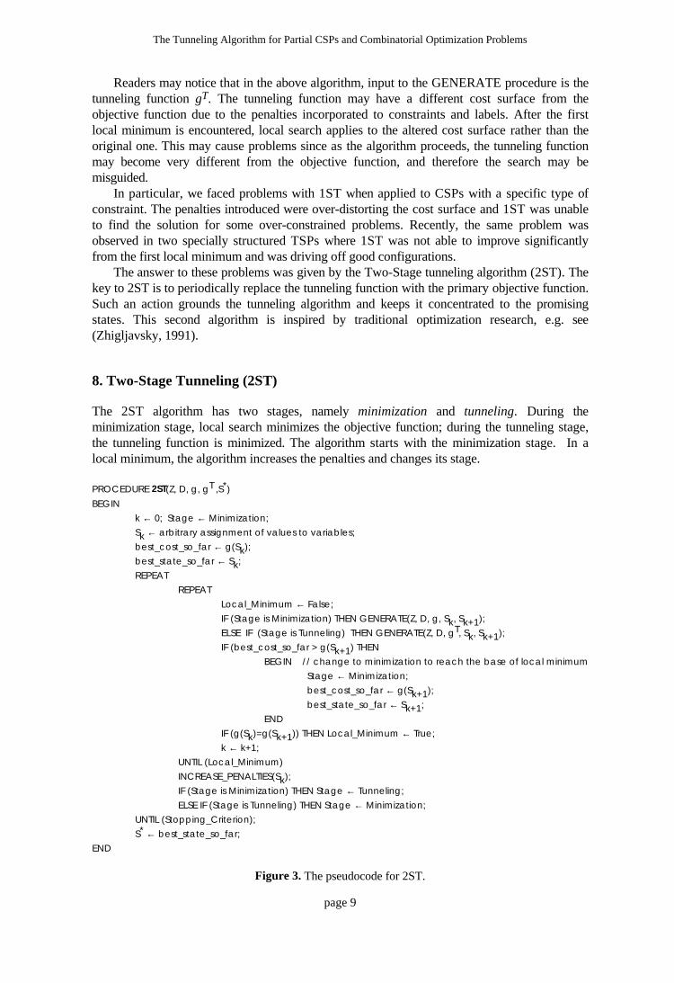
8. Two-Stage Tunneling (2ST)

The 2ST algorithm has two stages, namely minimization and tunneling. During theminimization stage, local search minimizes the objective function; during the tunneling stage,the tunneling function is minimized. The algorithm starts with the minimization stage. In alocal minimum, the algorithm increases the penalties and changes its stage.

PROCEDURE 2ST(Z, D, g, gT ,S*)

BEGIN

k ← 0; Stage ← Minimization;

Sk ← arbitrary assignment of values to variables;

best_cost_so_far ← g(Sk);

best_state_so_far ← Sk;

REPEAT

REPEAT

Local_Minimum ← False;

IF (Stage is Minimization) THEN GENERATE(Z, D, g, Sk, Sk+1);

ELSE IF (Stage is Tunneling) THEN GENERATE(Z, D, gT, Sk, Sk+1);

IF (best_cost_so_far > g(Sk+1) THEN

BEGIN // change to minimization to reach the base of local minimum

Stage ← Minimization;

best_cost_so_far ← g(Sk+1);

best_state_so_far ← Sk+1;

END

IF (g(Sk)=g(Sk+1)) THEN Local_Minimum ← True;

k ← k+1;


INCREASE_PENALTIES(Sk);

IF (Stage is Minimization) THEN Stage ← Tunneling;

ELSE IF (Stage is Tunneling) THEN Stage ← Minimization;


S* ← best_state_so_far;

END

Figure 3. The pseudocode for 2ST.


page 10

The aim of the tunneling stage is to help local search to escape local minima. However,since it is the objective function that matters, the algorithm uses the objective function once ithas escaped from a local minimum. Figure 3 gives the pseudocode for two-stage tunneling.

As we shall explain in the next section, care has been taken to ensure that the penaltiesincreased by the procedure INCREASE_PENALTIES are high enough to allow the algorithmto escape from the local minimum that the algorithm is currently in. If the amount of penalty istoo small, the algorithm will have to change between the minimization and tunneling stages anumber of times before escaping the local minimum.

9. The Mechanism of Penalties

Both the algorithms described rely on the INCREASE_PENALTIES procedure to modify thetunneling function in such a way that would enable them to escape from the local minimumstate. The modification increases penalties for some of the terms included in the tunnelingfunction which are present in the local minimum. In this section, we shall describe thismechanism in detail. As it has been mentioned before, these terms are either label costs orconstraint costs.

To recapitulate, each term that contributes to the tunneling function has a penalty assignedto it. At the beginning of the search all the penalties are equal to 0 and the tunneling function isequivalent to the objective one. Each time the local search algorithm descends to a localminimum, the procedure INCREASE_PENALTIES is called to increase certain penalties. Themain objective of doing so is not just to raise the cost surface in the local minimum but also toshape it in such a way that the algorithm will follow a trajectory towards states with lowercosts. Therefore, it is preferable to penalize constraints and labels with higher costs first7 . Thepenalty-updating mechanism must decide on the following two issues:

• The terms to be penalized;• The amount of penalty to be increased.

To make these decisions, the tunneling algorithm uses a simple heuristic based on frequencycounts and cost information. This heuristic, which will be described in the following sections,has been proved to be effective in problems studied so far.

9.1 Selecting the Terms to be Penalized (FCR Heuristic)

The selection of terms to be penalized is based on two criteria. The first is the contribution (i.e.cost) of a term (representing a constraint or label cost) to the objective function. The second isthe number of times (absolute frequency) that this term has been penalized in the past. For eachterm (constraint or label), the Frequency to Cost Ratio (FCR) is computed by the number oftimes a term has been penalized in the past divided by the cost of the term:

FCRFrequency

Cost= (Eq. 11)

7 A plausible assumption is that states in which high cost terms do not contribute to the objective function arelikely to be better. By penalizing the high cost terms, we enable local search to explore these more promisingstates.


page 11

A set MinFCR is constructed in the local minimum state S*. This set includes the terms that

• contribute positively to the objective function in S* (i.e. the terms which represent the costsof those violated constraints and selected labels); and

• have the minimum FCR value.

The PenalizeSet is a subset of MinFCR which contains the elements of MinFCR with thehighest primary cost. Thus, the overall selection procedure employs a min-max like operationwhere we penalize the elements with the maximum cost amongst those with the minimum FCRvalue.

Initially, the FCR values are all equal to 0. So the selection is made purely on the primarycosts. After the tunneling function has been modified, frequency counts are increased for thepenalized terms. Since frequency counts are divided by the cost, FCR values increase faster forlow cost elements than for high cost elements and therefore high cost elements get morechances to be penalized than the low cost elements. Nevertheless, low cost elements will still bepenalized if the high cost elements have been penalized enough number of times. In CSPs,where all the constraints have the same violation cost and considered hard, we can simplypenalize all the constraints violated in the local minimum without considering FCR values,which is what the basic GENET models do. In CSOPs, this mechanism allows us to selectalternative labels when no constraints are violated which means after a solution has beenreached, the algorithm is given a chance to find better solutions.

Ultimately, each term considered in the selection process corresponds to a tunnelingdirection. Penalizing the term will propel local search towards that direction. Essentially, thetunneling direction points to states where the corresponding term has no contribution to the costfunction. To diversify the search, it is better to follow tunneling directions not followed in pastlocal minima. This results in a sequence of 'conjugate' tunneling directions. Finding the globaloptimum may require the tunneling directions to be followed several times over several localminima. FCR aims to do that by providing a cost-regulated cycling of tunneling directionsstarting with the most promising ones and devoting effort proportionally to the cost of terms.Finally, penalizing all the terms in the PenalizeSet substantially speeds up the algorithm sincepropulsion is applied to more than one direction.

9.2 Amount of Penalty

When a term has been selected for penalizing, the amount of penalty to be added is determinedon the basis of information gathered by the GENERATE procedure presented in Section 5. Thegathering of information is not included in the pseudocode in order to keep it simple. In reality,for each variable xi, the algorithm records the difference (∆gv) between the minimum value (gv)and second minimum value returned by the objective function (or tunneling function, dependingon the input of GENERATE) for all possible labels for xi. This difference has to be overcomeby modifying the tunneling function if any change in the assignment of xi is to occur at all. Themain aim of keeping these differences is that they provide a rough estimation of the relativeheight of the shortest hills that surround the local minimum.

In general, PCSPs are problems where arbitrarily small or large discrepancies in cost mayoccur between the local minimum and its surrounding states. For example, consider oneextreme where a solution is found which only incurs a small assignment cost and all thesurrounding states violate hard constraints of the problem. On the other hand, situations arelikely where the cost of soft constraints violated in the local minimum is just slightly less thanthe total cost of violations incurring in the neighboring states. Therefore, the differencesgathered provide invaluable information to determine the scale of penalty amounts to beconsidered.


page 12

Another consideration comes from the nature of tunneling algorithm. In particular, thepenalty amount to be added to a constraint should be proportional to the primary cost of aconstraint such that the properties of the primary cost surface are carried along to the distortedsurface. Similarly, if the term which has been selected to be penalized represents a label, theamount of penalty to be added should reflect the primary cost of that label according to theobjective function.

The tunneling algorithm is built upon the binary GENET models, which have beendemonstrated to be successful for binary CSPs. In the binary models, all constraints haveprimary costs of 1. When a constraint is being violated in a local minimum, the cost of theviolated constraint is increased by 1. The landscapes occurring in binary GENET are relativelysmooth since the surrounding hills have heights that are a few times multiple of the primaryconstraint cost. The penalty amount in that case can be equal to the primary cost as it is inbinary GENET. In the first extreme case mentioned above, it is obvious that such a scheme isto fail in PCSPs since the surrounding hills may have cost hundreds or thousands of times thecost of the local minimum. If the penalty is only to increase by an amount equal to the primarycost, a large number of iterations could be needed before a change happens in the GENETnetwork. Thus to determine the penalty amount, we have to take into account both the cost ofthe term and the differences ∆gv gathered during the GENERATE procedure.

One potentially useful measure is the maximum difference ∆gv. This measure gives themaximum discrepancy between the local minimum and the closest neighboring states in alllocal search directions. An alternative measure is the minimum difference ∆gv. This measurecan be term dependent since each term is associated to a subset of the variables (e.g. constraint)and therefore the minimum is taken only amongst these variables. These two measurescombined with the cost of the term give the following two candidate formulas for the penaltyamount.

{ }{ }PenaltyAmount gv= max , maxcost ∆ (Eq. 12)

and

{ }{ }PenaltyAmount gv= max , mincost ∆ (Eq. 13)

The first formula (Eq. 12) guarantees that a change in the assignment of at least onevariable will occur, even if the term is the only that is penalized. The second formula (Eq. 13)guarantees the same but it does not assure that the term will stop contributing to the costfunction since that may be subject to changing the value of more than one variable. So which isthe best formula? A first choice could be (Eq. 12) which needs less computation since

{ }max ∆gv has to be computed only once for all terms. However, the amount of additional

penalty defined in (Eq. 12) is more than enough to make the network change state and thatpenalty excess may distort the landscape of the search space unnecessarily, and consequentlymislead the search. In the experiments, we used both formulas. It appears to be the case that(Eq. 12) performs better in landscapes with very steep hills while (Eq. 13) is more effectivewhere smoother landscapes are expected.

The pseudocode in Figure 4 summarizes the procedure for increasing the penalties wherePenaltym and Frequencym are set to 0 for all the terms in the beginning of 1ST or 2ST andthe PenaltyAmount is given either by (Eq. 12) or (Eq. 13).


page 13

PROCEDURE INCREASE_PENALTIES(State)

BEGIN

Tlabels ← set of labels in State with cost > 0;

Tconstraints ← set of constraints that are violated;

T ← Tlabels + Tconstraints;

MinFCR ← set of elements in T with minimum FCR value;

PenalizeSet ← elements in MinFCR with highest cost;

FOR each element m in PenalizeSet DO

BEGIN

Penaltym ← Penaltym + PenaltyAmount;

// PenaltyAmount is defined in (Eq. 12 or 13)

Frequencym ← Frequencym +1;

END

END

Figure 4. The INCREASE_PENALTIES procedure in pseudocode.

10. Experimentation and Results

Like most other stochastic search methods, the tunneling algorithm cannot guarantee to find theoptimal solution. The main target of the experimentation presented here was to providepractical evidence that the algorithm is capable of finding the optimal or near optimal solutionsreliably, subject to limited resources and stopping criterion. The objectives of the experimentswere to determine whether:

• tunneling advances over GENET's performance in CSPs;• tunneling is applicable to randomly generated PCSPs;• tunneling can face the challenge of real world CSOPs and PCSPs; and• tunneling can be used for tackling other combinatorial optimization problems.

To accomplish the objectives listed above, we conducted experiments on a diversified set ofproblems, which includes problems from the following categories:

• randomly generated general constraint satisfaction problems• hard graph coloring problems in the literature• randomly generated binary partial CSPs• real life CSOPs and PCSPs• traveling salesman problems

For CSPs, comparisons were carried out with original GENET, Min-Conflicts Hill Climbing(MCHC) (Minton et al. 1992) and GSAT (Selman & Kautz, 1993). Optimization problemswere taken from the literature and results were compared with the best solutions known so farwhenever they are available. Whenever the optimal solutions are known, the average solutionerrors of the tunneling algorithm are given.

10.1 Random General CSPs

Davenport et al. (1994) reported results for GENET on random general CSPs involving atmostconstraints. The atmost constraint type is extended from CHIP (Dincbas et al. 1988). It isuseful for modeling certain constraints imposed on resources in scheduling problems. Given aset of variables Var and a set of values Val, the atmost(N, Var, Val) constraint specifies that no


page 14

more than N variables from Var may take values from Val. The set of problems used in thispaper is the same as that in (Davenport et al. 1994). In summary, the problems have 50variables with a domain size of 10 each and randomly generated atmost constraints where N =3, |Var| = 5 and |Val| = 5. Problem groups with 400, 405, 410, ..., up to 500 atmost constraintswere generated. For each problem group, ten CSPs were generated. In order to test thereliability of the tunneling algorithm (i.e. how often it misses solutions), only soluble CSPswere chosen for comparison.

We tested 2ST against the MCHC and the GENET Stable1-Sideway model (which wasreferred to as GENET1 in (Davenport et al. 1994)) on this set of problems8 . Because of thestochastic nature of these algorithms, we ran each algorithm 10 times for each problem. Thelimit for each run was set to 10,000 iterations (1 iteration = 1 GENET cycle) for GENETStable1-Sideway model and for 2ST. The equivalent number of iterations for MCHC is500,000 since MCHC examines only one variable per iteration. If a solution is found within thegiven number of iterations then this is considered as a successful run. For 2ST, the cost of theconstraints and the penalty amount were all set to 1 and all the violated constraints werepenalized in a local minimum. Figure 5 illustrates the percentage of successful runs for thesealgorithms, which measures their relative reliability. Both 2ST and the GENET Stable1-Sideway model clearly out-perform MCHC. For tightly constrained CSPs, 2ST out-performsthe GENET Stable1-Sideway model see the right-hand end of the chart where thepercentage of successful runs declines faster for GENET than for 2ST.

Number of atmost constraints

Succ

essf

ul r

uns

(%)

0

10

20

30

40

50

60

70

80

90

100

400

405

410

415

420

425

430

435

440

445

450

455

460

465

470

475

480

485

490

495

500

MCHC

GENET

2ST

Figure 5. MCHC, GENET Stable1-Sideway, and 2ST on random general CSPs.

10.2 Hard Graph Coloring Problems

In this experiment, we tested 2ST on the four graph coloring problems from (Johnson et al.1991) which have been suggested to be hard problems. We compare the results from 2ST withthose from the GENET Stable1-Sideway model and GSAT, as they were reported in(Davenport et al. 1994). We counted a repair ("flip") for 2ST, each time the value of a variable

8 1ST is the same as GENET1 in CSPs.


page 15

was changed. The medians for the number of repairs, time and iterations are calculated over 10runs for each problem. Table 1 presents these results, which show that 2ST out-performs bothGENET and GSAT in terms of number of repairs and time.

Nodes Colors Median Number of Repairs Median Time9 Median number of

iterations

GSAT GENET 2ST GSAT GENET 2ST GENET 2ST

125 17 65,197,415 1,626,861 498,463 8.0h 2.6h 1.08h 524,517 131,385

125 18 65,969 7,011 4,949 30s 23s 17.6s 1,243 578

250 15 2,839 580 536 5s 4.2s 1.4s 15 12

250 29 7,429,308 571,748 338,571 1.8h 1.1h 1.1h 63,767 34,614

Table 1. GSAT, GENET, and 2ST on hard graph coloring problems.

10.3 Random Binary PCSPs

In order to examine the suitability of tunneling for Partial CSPs, we generated a set of randomproblems with soft binary constraints and assignment costs. The control parameters of theexperiment are the density and tightness of the binary constraints. The density is defined as theprobability of a pair of variables being constrained and the tightness is the probability of twolabels of two constrained variables being incompatible. The constraints were represented inmatrix format (Tsang, 1993) and we employed GENET's scheme for representing them (i.e.one constraint for each pair of incompatible values). Random costs in the range of 1 to 100were assigned to the labels and in the range of 1,000 to 10,000 to the constraints. Thisbasically means that the primary goal is to satisfy all the constraints, and the secondary goal isto choose low cost values (which is a reasonable thing to do in many scheduling problems). Theobjective function for all the problems is the combined cost of selected labels and violatedconstraints in the solution as given by (Eq. 9).

10.3.1 Design of Experiment

The randomly generated problems have 10 variables with domain size of 10. We varied theconstraint density from 0.1 to 0.9 by increments of 0.1. For each density level, we variedtightness from 0.1 to 0.9 by increments of 0.1. This resulted in 81 distinct density-tightnessconfigurations. Ten PCSPs were generated for each configuration, aggregating to a total of 810problems. We solved all the problems to optimality with a Branch and Bound algorithm similarto Partial B&B presented by (Freuder & Wallace, 1992), appropriately modified toaccommodate label and constraint costs. We tested 1ST and 2ST on the problems generated.Because of the stochastic nature of the tunneling algorithms, we ran each algorithm 10 timesfor each problem. The stopping criterion was set to 10,000 iterations. The FCR heuristic usedfor the selection of terms to be penalized and the penalty amount was specified by (Eq. 12).

10.3.2 Evaluation of Results

The main observation in this experiment is find out how close tunneling algorithms can get tooptimal solutions in binary PCSPs. The performance of the tunneling algorithms are measured

9 The experiments on the graph coloring problems were conducted on a Sun Microsystems Sparc ClassicWorkstation with a 2ST implementation in C++. The same settings were used as in (Davenport et al. 1994).


page 16

by the relative solution error also mentioned as percentage excess, which is defined by thefollowing formula:

Errorg g

gopt

opt

(%)*

=−

×100 (Eq. 14)

where g* is the cost of the solution returned by the algorithm within a limit of iterations andgopt the cost of the optimal solution. Analysis of variance (ANOVA) (Mendenhall & Sincich,1992) was conducted on the 1ST and 2ST results. The dependent variable is the solution errorand the three factors involved are:

• Algorithm: 1ST, 2ST (2 levels)• Density: 0.1, 0.2,..., 0.9 (9 levels)• Tightness: 0.1, 0.2,..., 0.9 (9 levels)

The main objective of the analysis is to evaluate 1ST and 2ST on the basis of error and also todetermine interactions between the factors involved in the experiment. Table 2 shows theresults from the ANOVA test.

Source of Variation Degrees of Freedom F p-valueAlgorithm 1 6.74 0.0094

Density 8 1.15 0.3269Tightness 8 4.04 0.0001

Algorithm*Density 8 1.08 0.3701Algorithm*Tightness 8 3.78 0.0002

Density*Tightness 64 2.35 0.0001Algorithm*Density*Tightness 64 1.72 0.0003

error 16199 - -

Table 2. Results of ANOVA test with dependent variable the solution error.

As we can see from the above table the effect on the solution error due to the algorithms isstatistically significant (p=0.0094). Another significant factor is the tightness of the constraints(p=0.0001) while the density of the constraints alone or combined with the algorithms are notstatistically significant (p=0.3269 and p=0.3701, respectively). We compared further 1ST and2ST on the basis of solution error and time using Tukey's method for multiple comparisons(Mendenhall & Sincich, 1992). The results presented in Table 3 show that the 1ST and 2STmeans on both solution error and time are significantly different.

Mean Solution Error Mean Time in CPU seconds10

1ST 2ST 1ST 2ST0.03292% 0.01322% 6.87 sec 2.96 sec

Table 3. Performance comparison between 1ST and 2ST on PCSPs.

In fact, 2ST failed to find the optimal solution in only 51 out of 8100 runs while 1ST failed208 times for the same number of runs. In those cases, near-optimal solutions were discoveredby both algorithms. Figure 6 graphically illustrates the problems in which 1ST and 2ST failed.It shows that 1ST faced difficulties in tight PCSPs while 2ST in problems around the phase

10 The experiments in random binary PCSPs were conducted on a Sun Microsystems Sparc Classic with 1ST,2ST and B&B implemented in C++.


page 17

transition region (Smith, 1994). The overall performance of 2ST is significantly better thanthat of 1ST (note the change of scales in the z-axis in the timing and error).

Aver. Time (sec.) Aver. Time(sec.)

2ST Algorithm

Aver. Error(%)

2ST AlgorithmAver. Error (%)

1ST Algorithm

0.900.70

0.500.30

0.10Tightness Density

0.900.70

0.500.30

0.10

0.900.70

0.500.30


0.900.70

0.500.30

0.10

0.900.70

0.500.30


0.900.70

0.500.30

0.10

0.900.70

0.500.30


0.900.70

0.500.30

0.10

1ST Algorithm

0.54

0.41

0.27

0.14

0.00

0.27

0.20

0.14

0.07

0.00

35.67

23.79

11.91

0.00

9.78

6.52

11.91

0.00

Figure 6. The surfaces11 of solution error and time for 1ST and 2ST.

Note that the size of the problems tested is limited by the combinatorial explosion problemfaced by the Partial B&B (Wallace & Freuder, 1993), which takes many hours to solveproblems with 20 variables even when it provided with initial bounds generated by 2ST. Suchresults give justification for using stochastic methods such as the tunneling algorithm forPCSPs.

10.4 The Radio Link Frequency Assignment Problem A Real Life PCSP

Randomly generated problems with known properties are useful for evaluating algorithmperformance and therefore helping to guide the development of algorithms. However, we wouldalso like to know how well the tunneling algorithms will perform in large CSOPs and PCSPs inreal life applications.

We have tested the tunneling algorithms on the Radio Link Frequency AssignmentProblem, which was abstracted from the real life application of assigning frequencies (values)to radio links (variables). Eleven instances of RLFAPs, which involve various optimizationcriteria, were made publicly available by the French Centre d'Electronique l'Armament(RLFAP, 1994). Two different types of binary constraints may be involved in these RLFAPs:

• The absolute difference between two frequencies must be greater than a given number k(i.e. for two frequencies X and Y, |X - Y| > k);

• The absolute difference between two frequencies must be exactly equal to a given number k(i.e. for two frequencies X and Y, |X - Y| = k).

11 Inverse distance interpolation used.


page 18

Along with the problems publicized, the best solutions known so far (some of which wereknown to be optimal) were given. These solutions were found by tree-search algorithms, graphcoloring algorithms and other methods. We applied both 1ST and 2ST to all the publishedRLFAPs instances. In the following sections, we shall first describe the optimization criteria ofthe problems; then we shall present our results.

10.4.1 Optimization Criteria

The problems involve both hard and soft constraints. If all the constraints can be satisfied theneither:

• (C1) the solution which assigns the fewest number of different values to the variables,• (C2) or the solution which largest assigned value is minimal

is preferred. For insoluble problems, violation costs are defined for the constraints.Furthermore, for some insoluble problems, default values are defined for the variables. If anyof the default values is not used in the solution returned, then a predetermined mobility costapplies.

10.4.2 Problem Modeling

A. PCSPs

Modeling RLFAPs as PCSPs is straightforward. The primary constraint costs are set equal tothe given violation costs. The primary label costs are all set to 0 for the default labels for thevariables and to the mobility cost for all the other labels for each variable.

B. CSOPs

The two optimization criteria (C1) and (C2) are difficult to be modeled since both of them arenon-linear the cost of choosing a label depends on the values that other variables are takingin the current network state. To encourage the network to move towards the optimal solutions,these costs must be reflected in the primary label costs. We shall first explain how to model(C1) in our objective function.

The label cost of the label l = <x, v> in the network state S is defined as follows:

( )l S NVar NVarv v= − ' (Eq. 15)

where NVar the total number of variables in the problem and NVarv' the number of variables

that are assigned the value v in state S. The tunneling cost corresponding to (Eq. 15) is definedas follows:

( )l S NVar NVar penaltyv v v= − +' (Eq. 16)

where penaltyv is defined for each possible value in the union of all the domains rather thanseparately for each individual label.

Firstly, the hard constraints of all the problems (PCSPs and CSOPs) were assigned highviolation costs. Therefore, soft constraints and label costs are effectively ignored until the hardconstraints are satisfied. In a local minimum, if hard constraints are violated, we penalize themall. The penalty amount used is defined in (Eq. 13).; i.e. the minimal penalty to enable thenetwork to change state is applied to the terms selected for penalizing.


page 19

If all the hard constraints are satisfied then the FCR heuristic considers the label costsdefined in (Eq. 15). In the selection, we exclude values not used by any of the variables becausethey cannot affect the cost of the local minimum once they are not used. Since a value may beused by many variables, in order to reduce the computational effort, we use (Eq. 12) for thesepenalty amounts.

The second criterion (C2) can be modeled in a similar way, but since criterion (C2) is onlyinvolved in one of the RLFAPs which solved as a CSP, we shall not elaborate it here. Theresults on running the 1ST and 2ST algorithms on the RLFAPs will be shown in the followingsections12 .

10.4.3 Problems 1,2,3,11 - Soluble Problems modeled as CSOPs

These problems have been modeled as CSOPs. The objective is to find the solution whichminimizes the criterion (C1) defined above. We ran 1ST and 2ST ten times on each problemwith the stopping criterion set to 20,000 iterations. The results obtained are consistent with thebest solutions known so far. In Problem 2 the tunneling variants frequently found thepublicized optimal solution. Problem 11 was initially thought to be insoluble and therefore wastreated as a PCSP. It later turned out that the problem was soluble. Therefore, we proceededfurther by treating problem 11 as a CSOP subject to criterion (C1). Table 4 summarizes theresults obtained by running 1ST and 2ST on these four problems. It is worth emphasizing thatthe large number of variables and values involved in all of these problems prevents any knowncomplete search algorithm from succeeding in solving them in reasonable time.

Problem Number of

Variables

Number of

Constraints

Cost of Best Solution

Known

Algorithm Median

Cost

Min Cost Max

Cost

Aver. Time

(CPU sec.)

Aver.

Iterations

1 916 5,548 16 1ST 18 16 48 123 655

2ST 20 20 26 514 2,636

2 200 1,235 14 (optimal) 1ST 14 14 16 5 120

2ST 14 14 18 21 486

3 400 2,760 16 1ST 16 16 18 181 1,964

2ST 17 16 20 293 3111

11 680 4,103 Solution violates

0 constraints

1ST 41 32 Not

solved

512 3,677

2ST 43 30 Not

solved

360 2,575

Table 4. RLFAP - Problems 1, 2, 3, and 11.

10.4.4 Problems 4,5 - Soluble Problems modeled as CSPs

Problem 4 requires optimization with respect to criterion (C1) and some of the variables in itare given default values. The optimization criterion for Problem 5 is (C2). Both 1ST and 2STfailed to solve these problems when they were treated as CSOPs. We believe that this failurewas caused by the irregularity of the cost surface due to the costs and penalties added to theobjective function from the optimization criteria which prohibited sideways moves. This doesindicate that there is room for improvement for the tunneling algorithms. However, in ignoringthe optimization criteria and attempting to solve these two problems as CSPs, 1ST and 2STfound solutions in all their ten runs within 20,000 iterations. Moreover, all the solutionshappened to be optimal with respect to the corresponding criteria. Detailed results are presentedin Table 5.

12 The experiments on RLFAPs were conducted on DEC Alpha machines with 1ST and 2ST written in C++.


page 20

Problem Number of

Variables

Number of

Constraints

Cost of Best

Solution Known

Algorithm Median

Cost

Min

Cost

Max

Cost

Aver. Time

(CPU sec.)

Aver.

Iterations

4 680 3,967 46 (optimal) 1ST 46 46 46 5 58

2ST 46 46 46 6 72

5 400 2,598 792 (optimal) 1ST 792 792 792 115 1,181

2ST 792 792 792 155 1,628

Table 5. RLFAP - Problems 4 and 5.

10.4.5 Problems 6,7,8 - Insoluble Problems modeled as PCSPs

These problems have no known solutions which satisfy all the constraints. So they were treatedas PCSPs. We solved the problems using the FCR heuristic and penalty amounts given by (Eq.13). The stopping criterion was set to 20,000 iterations. Each problem was run ten times by thetunneling algorithm and the results are presented in Table 6. In contrast to the previousproblems, 2ST found better solutions than 1ST. They both found far better solutions than thebest known solutions so far in Problems 7 and 8.

Problem Number of

Variables

Number of

Constraints

Cost of Best

Solution Known

Algorithm Median

Cost

Min

Cost

Max

Cost

Aver. Time

(CPU sec.)

Aver.

Iterations

6 200 1,322 6,787 1ST 5,514 4,492 6,842 77 1,613

2ST 4,661 3,702 5,253 402 8,332

7 400 2,865 2,545,752 1ST 63,162 47,104 1,063,987 1,001 9,621

2ST 49,977 41,705 1,092,497 985 9,427

8 916 5,744 1,772 1ST 396 354 438 1,505 7,135

2ST 384 317 427 1,867 8,776

Table 6. RLFAP - Problems 6, 7, and 8.

10.4.6 Problems 9,10 - PCSPs involving assignment costs

The problems 9 and 10 are PCSPs in which default values are provided for some of thevariables. A number of variables must take these values while others may be assignedalternative values at certain costs (mobility costs). The sizes of these mobility costs arecomparable to constraint violation costs. We modeled mobility costs in the way that isdescribed in Section 10.4.2. We ran 1ST and 2ST five times on each problem up to 20,000iterations with penalty amounts given by (Eq. 12). We have to admit here that the quality ofsolutions was much inferior for less generous penalty amounts like those determined by (Eq.13). Table 7 summarizes the results of these experiments. Results by tunneling algorithm inProblem 9 were better than the best results found so far, but they were less impressive inProblem 10.

Problem Number of

Variables

Number of

Constraints

Cost of Best

Solution Known

Algorithm Median

Cost

Min Cost Max

Cost

Aver. Time

(CPU sec.)

Aver.

Iterations

9 680 4103 22,136 1ST 15,760 15,716 15,832 577 5211

2ST 15,755 15,721 15,889 1081 9725

10 680 4103 21,552 1ST 31,518 31,517 31,521 576 5135

2ST 31,520 31,517 31,618 332 2985

Table 7. RLFAP - Problems 9 and 10.


page 21

10.4.7 Evaluation of Results on RLFAP

In almost every instance of the publicized RLFAP (except Problem 10), the tunnelingalgorithms managed to find at least as good solution as the best solutions known so far. Therunning times required for these problems, which involved from 200 up to 916 variables, variedfrom a few seconds for the small CSOPs to less than an hour for the large PCSPs. Given thesizes and difficulty of the problems, we believe the times required by the tunneling algorithmswere reasonable. Unfortunately, no information was given about the times required to find thebest solutions publicized. In all the runs, very good solutions were available within a very shortperiod of time. This makes the tunneling algorithms suitable for (time) resource boundedapplications where early good solutions are welcome and further optimization is preferredwhenever time allows. It is worth pointing out that the tunneling algorithm is a generalalgorithm. Only minor adaptations were required for it to be applied to the RLFAP, yet resultsobtained by it were comparable to, if not better than, the best known results so far.

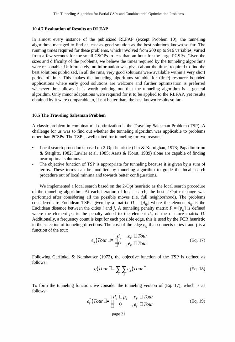
10.5 The Traveling Salesman Problem

A classic problem in combinatorial optimization is the Traveling Salesman Problem (TSP). Achallenge for us was to find out whether the tunneling algorithm was applicable to problemsother than PCSPs. The TSP is well suited for tunneling for two reasons:

• Local search procedures based on 2-Opt heuristic (Lin & Kernighan, 1973; Papadimitriou& Steiglitz, 1982; Lawler et al. 1985; Aarts & Korst, 1989) alone are capable of findingnear-optimal solutions.

• The objective function of TSP is appropriate for tunneling because it is given by a sum ofterms. These terms can be modified by tunneling algorithm to guide the local searchprocedure out of local minima and towards better configurations.

We implemented a local search based on the 2-Opt heuristic as the local search procedureof the tunneling algorithm. At each iteration of local search, the best 2-Opt exchange wasperformed after considering all the possible moves (i.e. full neighborhood). The problemsconsidered are Euclidean TSPs given by a matrix D = [dij] where the element dij is theEuclidean distance between the cities i and j. A tunneling penalty matrix P = [pij] is definedwhere the element pij is the penalty added to the element dij of the distance matrix D.Additionally, a frequency count is kept for each possible edge, this is used by the FCR heuristicin the selection of tunneling directions. The cost of the edge eij that connects cities i and j is afunction of the tour:

( )e Tourd e Tour

e Tourij

ij ij

ij

=∈∉

,

,0 (Eq. 17)

Following Garfinkel & Nemhauser (1972), the objective function of the TSP is defined asfollows:

( ) ( )g Tour e Tourijji

= ∑∑ (Eq. 18)

To form the tunneling function, we consider the tunneling version of (Eq. 17), which is asfollows:

( )e Tourd p e Tour

e TourijT ij ij ij

ij

=+ ∈

∉

,

,0 (Eq. 19)


page 22

The tunneling function for TSP is defined as follows:

( ) ( )g Tour e TourTijT

ji

= ∑∑ (Eq. 20)

In the TSP, the terms of the objective function to be modified are the edge lengths. Oncethe terms for modification have been identified, the basic mechanism of tunneling is the same asthe one for PCSPs. 1ST and 2ST use 2-Opt as the basic local search procedure. Through thetunneling function, 2-Opt sees the edge lengths as given by (Eq. 19). Due to penalty terms,edges may be considered longer than they really are. In a local minimum (i.e. there is no 2-change that improves the tour), an edge is selected using the FCR heuristic presented in Section9.1 and an amount equal to the primary distance is added to its penalty. In tie situations, onlyone edge was penalized. The new penalties force 2-Opt to consider moves which were notconsidered before, thus escaping from the local minimum.

Since the TSP is not modeled as a PCSP, the pseudocode of modified 1ST (modified fortackling TSPs) is given in Figure 7.

PROCEDURE 1ST-TSP(g, gT, Tour*)

BEGIN

k ← 0;

Tourk ← arbitrary legal tour;

best_cost_so_far ← g(Tourk);

best_tour_so_far ← Tourk;

REPEAT

REPEAT

2-Opt(gT, Tourk, Tourk+1);

IF (best_cost_so_far > g(Tourk+1) THEN

BEGIN

best_cost_so_far ← g(Tourk+1);

best_tour_so_far ← Tourk+1;

END

k ← k+1;


INCREASE_PENALTIES(Tourk);


Tour* ← best_tour_so_far;

END

Figure 7. The 1ST algorithm for the Traveling Salesman Problem.

The basic difference between this algorithm, which we call 1ST-TSP, and the standard 1ST forPCSPs is in the use of 2-Opt instead of the GENERATE procedure. Similar modificationswere made for 2ST, resulting in the algorithm 2ST-TSP which will not be elaborated here.

10.5.1 Experimentation with TSPs

In this section, we shall present results for 1ST-TSP and 2ST-TSP on a set of ten well-studiedTSP problems where the optimal solutions are known. These problems are from TSPLIB(Reinelt, 1991), a library of TSP problems. The stopping criterion was set to 100,000iterations. Ten runs were made for each problem. Table 8 presents the results of our runs.


page 23

ProblemIdentity

No. Cities Average Excess (%)(Eq. 14)

Average Time(CPU seconds13 )

Optimal Runs(out of 10)

Aver.No. Iterations

1ST 2ST 1ST 2ST 1ST 2ST 1ST 2ST

eil51 51 0.00 0.09 4.94 21.8 10 6 3006 13383eil76 76 0.00 0.11 20.3 43.5 10 5 5629 11952eil101 100 0.00 0.10 82.3 41.9 10 5 12537 6380

kroA100 100 0.09 0.09 135.8 305.6 2 4 21185 47341kroC100 101 0.00 0.27 196.0 145.8 10 2 30782 23036lin105 105 0.16 0.00 73.6 17.4 4 10 10577 2522

kroA150 150 0.09 0.37 779.2 1111.8 2 1 41598 53670kroA200 200 0.43 0.65 2176.1 1062.9 0 0 60468 30370lin318 318 1.05 1.42 4617.7 5403.5 0 0 50412 57679pr439 439 0.89 1.10 9866.4 8171.8 0 0 55745 47224

Table 8. Table of results for the Traveling Salesman Problem.

The algorithms in all the runs improved the solutions found by 2-Opt alone (i.e. the firstlocal minima). If enough time was given the algorithms were able to find the optimal solution inmost problems. Between the algorithms, 1ST-TSP had a better overall performance than 2ST-TSP. Figure 8 shows the fluctuation of the cost during the 500 iterations of 1ST-TSP on aproblem with 51 cities. As can be seen from the figure, after the initial steep drop in cost, thealgorithm visited solutions with near-optimal costs. Eventually, it obtained the optimal cost.

Iteration

Tou

r L

engt

h

0

200

400

600

800

1000

1200

1400

1600

0 100 200 300 400 500

Figure 8. The cost of the solutions generated in the first 500 iterations of 1ST for a TravelingSalesman Problem with 51 cities.

Note that both 1ST-TSP and 2ST-TSP alter the cost function only after the first localminimum is reached and therefore in the worst case their performances are at least as good as2-Opt. This is not necessarily the case for other methods which are also built upon 2-Opt, forexample tabu search and simulated annealing. Furthermore in tunneling, no parameter otherthan the upper limit of iterations is necessary to be specified (unlike some other methods suchas genetic algorithms). It must be emphasized that the experimentation with TSPs presented issubject to improvement since alternative edge selection heuristics (other than FCR) can bedevised and approximate 2-Opt based local search procedures might be used. Discussion ofsuch improvements will be left for another occasion.

13 TSP experiments were conducted on DEC Alpha Machines with 1ST-TSP and 2ST-TSP written in DEC C++.


page 24

11. Future Work

Further study will focus on analyzing when the tunneling algorithm will perform better thanother methods, why and how it can be improved. In order to improve the efficiency andeffectiveness of the algorithm, the following issues will be look at:

• Penalty Amounts• Selection Procedure• Termination Criterion

The efficiency of the algorithm is strongly related to the first two decisions. Applying largepenalties in general will speed up the algorithm at the risk of burying optimal solutions amonginferior solutions. Low penalties have the opposite effect of slowing down the algorithm butreducing such risks. The FCR heuristic presented in this paper has worked well for theproblems studied so far. However, different selection procedures may be more efficient for thesame or other kinds of problems. Finally, for the termination criterion, more sophisticatedschemes may be explored.

12. Summary and Conclusions

Many real life problems can be formulated as partial constraint satisfaction problems (PCSPs),which involves the assignment of values to variables satisfying a set of constraints andoptimizing according to a specified objective function whenever possible.

GENET is a connectionist approach to constraint satisfaction. In this paper, we haveintroduced the tunneling algorithm, which is extended from GENET to include optimization,for solving PCSPs. We have also demonstrated the generality of the tunneling algorithm byapplying it to a combinatorial optimization problem, namely the TSP.

Results so far indicate that the tunneling algorithm is applicable to a variety of problems. Ithas been shown to be robust in satisfiability problems: it managed to solve the tested problemsin more cases than some of the best algorithms published so far (namely the MCHC, GSATand the GENET Stable1-Sideway Model). It has also been demonstrated to be effective onoptimization problems: in applying it to a number of publicly available RLFAPs and TSPs, ithas consistently been able to find solutions with quality which is as good as, and sometimesmuch better than, that in the best solutions found so far. Moreover, we found it relatively easyto adapt the algorithm to different applications.

Despite the incompleteness of the tunneling algorithm, it had no difficulties in producingoptimal solutions repeatedly in a high proportion of the problems tested within reasonable time.Therefore, this algorithm should be a powerful tool for tackling problems which backtrack-based algorithms find intractable.

To summarize, the tunneling algorithm has been shown to be a robust and effectivealgorithm for constraint satisfaction and optimization problems.

Acknowledgments

We would like to thank the Centre d'Electronique l'Armament for making available the RLFAPinstances which initiated our development of the tunneling algorithm and The British TelecomResearch Laboratories for making available a number of real instances of network schedulingproblems which lead us to the development of the 2ST scheme. Andrew Davenport provided uswith his implementation of the GENET Stable1-Sideway model and its results in tackling thegraph coloring problems. Both Andrew Davenport and James Borrett commented on an earlier


page 25

version of this paper. The Computing Service of the University of Essex gave us access to theDEC Alpha machines which helped us to carry out the experiments. This project and ChrisVoudouris are funded by the EPSRC grant (GR/H75275).

References

Aarts, E., & Korst, J. (1989). Simulated Annealing and Boltzmann Machines. New York:John Wiley & Sons.

Barto A. G., Sutton R. S., & Anderson C. W. (1983). Neurolike adaptive elements that cansolve difficult learning problems. IEEE Transactions on Systems, Man and Cybernetics,13, 834-846.

Davenport A., Tsang E., Wang C. J., & Zhu K. (1994). GENET: A connectionist architecturefor solving constraint satisfaction problems by iterative improvement. In Proceedings ofAAAI-94, 325-330.

Dincbas, M., Van Hentenryck, P., Simonis, H., Aggoun, A., & Graf, T. (1988). Applicationsof CHIP to industrial and engineering problems. In First International Conference onIndustrial and Engineering Applications of AI and Expert Systems.

Freuder, E. C., & Wallace, R. J. (1992). Partial constraint satisfaction. Artificial Intelligence,58, 21-70.

Garfinkel, R. S., & Nemhauser, G. L. (1972). Integer Programming. New York: John Wileyand Sons.

Glover, F. (1989). Tabu search Part I. Operations Research Society of America(ORSA)Journal on Computing, Vol. 1, 109-206.

Glover, F. (1990). Tabu search Part II. Operations Research Society of America(ORSA)Journal on Computing, Vol. 2, 4-32.

Johnson, D., Aragon, C., McGeoch, L., & Schevon, C. (1991). Optimization by simulatedannealing: an experimental evaluation, part II, graph coloring and number partitioning.Operations Research, 39(3), 378-406.

Kirkpatrick, S., Gelatt, C. D., & Vecchi, M. P. (1983). Optimization by simulated annealing.Science, 220, 671-680.

Lawler, E. L., Lenstra, J. K., Rinnooy Kan, A. H. G., & Shmoys D. B. (Eds.) (1985). TheTraveling Salesman Problem: A guided tour in combinatorial optimization. Chichester:John Wiley & Sons.

Levy, A.V., & Montalvo, A. (1985). The tunneling algorithm for the global minimization offunctions. SIAM Journal on Scientific and Statistical Computing, 6, No. 1, 15-29.

Lin, S., & Kernighan, B. W. (1973). An effective heuristic algorithm for the Travelingsalesman problem. Operations Research, 21, 498-516.

Mendenhall, W., & Sincich, T. (1992). Statistics for engineering and the sciences - 3rd ed.New York: Maxwell Macmillan International.


page 26

Minton S., Johnston, M.D., Philips, A. B., & Laird, P. (1992). Minimizing conflicts: aheuristic repair method for constraint satisfaction and scheduling problems. ArtificialIntelligence, 58, 161-205.

Morris, P. (1993). The breakout method for escaping from local minima. In Proceedings ofAAAI-93, 40-45.

Papadimitriou, C. H., & Steiglitz, K. (1982). Combinatorial Optimization: Algorithms andComplexity. Englewood Cliffs, NJ: Prentice-Hall.

Reinelt, G. (1991). A Traveling Salesman Problem Library. Operations Research Society ofAmerica(ORSA) Journal on Computing, Vol. 3, 376-384.

RLFAP (1994). The RLFAP problems are available from [email protected]. To getmore information and the problems send the command "get csp-list CELAR.blurb" to theabove listserver. Problems used in our tests were obtained on March 1994.

Selman, B., & Kautz, H. A. (1993). Domain dependent extensions to GSAT: Solving largestructured satisfiability problems. In Proceedings of the 13th International JointConference on Artificial Intelligence, 290-295.

Selman, B., Levesque, H. J., & Mitchell, D. G. (1992). A new method for solving hardsatisfiability problems. In Proceedings of AAAI-92, 440-446.

Selman B., Kautz H. A., & Cohen B. (1994). Noise strategies for improving local search. InProceedings of AAAI-94, 337-343.

Smith, B., M. (1994). Phase transition and the mushy region in constraint satisfactionproblems. In Proceedings of 11th European Conference on Artificial Intelligence, 263-267.

Tsang, E. (1993). Foundations of Constraint Satisfaction. London: Academic Press.

Wallace R. J., & Freuder E. C. (1993). Conjunctive Width Heuristics for Maximal ConstraintSatisfaction. In Proceedings of AAAI-93, 762-768.

Wang, C. J., & Tsang, E. (1991). Solving constraint satisfaction problems using neural-networks. In Proceedings of IEE Second International Conference on Artificial NeuralNetworks, 295-299.

Wang, C. J., & Tsang, E. (1992). A cascadable VLSI design for GENET. In InternationalWorkshop on VLSI for Neural Networks and Artificial Intelligence, Oxford.

Whittle P. (1971). Optimization under Constraints: Theory and Applications of NonlinearProgramming. London: John Wiley & Sons.

Zhigljavsky, A. A. (1991). Theory of Global Random Search. London: Kluwer AcademicPublishers.

The Tunneling Algorithm for Partial CSPs and …The Tunneling Algorithm for Partial CSPs and...

Documents

Transcript of The Tunneling Algorithm for Partial CSPs and …The Tunneling Algorithm for Partial CSPs and...