1

The Trouble with Harrod: the fundamental instability of the

warranted rate in the light of the Sraffian Supermultiplier

Franklin Serrano, Fabio Freitas and Gustavo Bhering*,†

Federal University of Rio de Janeiro

ABSTRACT

The paper discusses Harrod’s “principle of fundamental instability” of growth at the warranted rate,

using the Sraffian Supermultiplier model, together with Hicks’s notions of “static” and “dynamic”

stability, which are related to the distinction between the direction versus the intensity of a

disequilibrium adjustment. We explain why growth at Harrod’s warranted rate is fundamentally or

statically unstable. We then show how the autonomous demand component in the Sraffian

Supermultiplier eliminates Harrodian instability and that the dynamic stability of the supermultiplier

depends on the marginal propensity to spend remaining lower than one during the adjustment, a

modified “Keynesian stability” condition.

1 INTRODUCTION

The “Fundamental Instability” of Harrod’s (1939, 1948, 1973) “warranted rate of growth”

has, for long, been seen as an obstacle in the development of satisfactory demand led growth

models based on the “marriage between the multiplier and the accelerator” (i.e., those in

which total capacity generating business investment is in the long run explained by the capital

stock adjustment principle or “accelerator” in a broad sense). This paper aims to clarify the

economic meaning and some important theoretical implications of Harrod’s “principle of

fundamental instability”. For this purpose, we use the theoretical results provided by the

Sraffian Supermultiplier model (Serrano 1995a, 1995b), together with Hicks’s notions of

* Corresponding author: Franklin Serrano, e-mail:franklinserrano@gmail.com. † Acknowledgements ...

2

“static” and “dynamic” stability (Hicks, 1965), the latter being related to the distinction

between the direction versus the intensity of a disequilibrium adjustment.

Our analysis will proceed in two successive steps. First, we explain why growth at Harrod’s

warranted rate is indeed fundamentally or statically unstable under very general conditions.1

Next, we show why we think the Sraffian Supermultiplier2 presents a satisfactory solution

for the apparent incompatibility between demand led growth models and capacity generating

private investment being driven by the capital stock adjustment principle.

We also provide new mathematical proofs in discrete time of both the fundamental or static

instability of Harrod’s warranted rate of growth and of sufficient conditions for the dynamic

stability of the Sraffian Supermultiplier. We opted for a discrete time analysis for two

reasons. First, to make the mathematical analysis match the sequential, period after period,

discussion of what happens during the adjustment process both in the Harrodian and the

Sraffian Supermultiplier models. Secondly, because we know that continuous time proofs do

not give exact results for discrete period models, as they involve approximations that drop

out some interaction terms. We show that the economic meaning of the dynamic stability

condition for the Sraffian Supermultiplier is the same as in the continuous time case, namely,

that the marginal propensity to spend must remain lower than one during the adjustment

1 In this paper we are not concerned with the other problem pointed by Harrod, that is, the reconciliation of the

warranted rate of growth and a “natural rate” of growth given by the sum of exogenous rates of growth the labor

force and its productivity. 2 This model is characterized by distribution being exogenous (and determined along Sraffian lines), investment

being totally induced by the adjustment of capacity to demand and the importance of autonomous demand

components that do not create capacity for the private sector of the economy. These hypotheses were largely

inspired by the work of Garegnani (1962), which explains why the model was called Sraffian Supermultiplier

in Serrano (1995a, 1995b). Recently, Cesaratto (2016) has discovered that the idea of adapting Hicks’s (1950)

trade cycle Supermultiplier for the analysis of the trend of demand led growth driven by autonomous demand

was first introduced by Ackley (1963) in an econometric model developed for the Italian economy and

published only in Italian. The latter work was probably influenced by discussions relating to Garegnani (1962).

Recently, chapters III and IV of the latter work has been published in English as Garegnani (2015).

3

process. However, we also show that, in a discrete time specification, the exact value of the

stability condition is different. In fact, for any given growth rate of autonomous demand, the

marginal propensity to spend is now a bit larger and thus the maximum rate of growth of

autonomous demand compatible with dynamically stable demand led growth is slightly lower

than in the continuous time proofs available in the literature.3

The rest of the paper is organized as follows. In section 2 we present, very briefly, Hicks’s

notions of static and dynamic stability. In section 3 we discuss the meaning of Harrod’s

warranted rate and show that growth at this rate is indeed fundamentally or statically unstable,

as the adjustment always goes in the wrong direction. In section 4 we discuss the Sraffian

Supermultiplier and show that while the model is statically or fundamentally stable, it may

be dynamically stable or unstable depending on the intensity of the reaction of investment to

demand. In section 5 we present some brief final remarks. Two appendices contain,

respectively, discrete time formal proofs of Harrod’s fundamental (or static instability) and

a set of sufficient conditions for the dynamic stability of the Sraffian Supermultiplier.

2 HICKS ON “STATIC” AND “DYNAMIC” INSTABILITY

For Hicks, the distinction between “static” and “dynamic” instability relates to the direction

and intensity of the disequilibrium adjustment process, respectively. Thus, an equilibrium is

statically unstable if the disequilibrium adjustment leads the economic system in the “wrong”

direction, away from its equilibrium state, independently of the intensity (or speed) of the

adjustment process. However, even an equilibrium that is “statically” stable can still be

3 Continuous time formal proofs of the dynamic stability of the autonomous demand supermultiplier can be

found in Allain (2015), Dutt (2015), Freitas & Serrano (2015) and Pariboni (2015).

4

“dynamically” unstable, if the adjustment process is too intense so as to lead to a chronic

overshooting of the equilibrium position through undamped cycles. “Static” stability is thus

a necessary, but not sufficient condition for “dynamic” stability. On the other hand, a

“statically” unstable model is thus inherently unstable.

In a long footnote in Hicks (1965, p. 18, fn. 2)4 clarifies these concepts with the simple

example of a Neoclassical partial equilibrium analysis of a market with a given supply and

demand curve. In this context, if the resulting excess demand (i.e., demand minus supply)

function is negatively sloped the model is statically stable. On the other hand, if for some

reason the excess demand function is positively sloped, the model is statically and thus

inherently unstable. However, assuming that the excess demand function is well behaved and

negatively sloped is not sufficient to ensure dynamic stability. Indeed, if the market price

reaction to excess demand is not continuous but happens in discrete or lumpy jumps, for

sufficiently high value of the parameters one may find that the equilibrium is dynamically

unstable. In this case, although static conditions points the adjustment process in the right

direction as defined by economic theory, there can be an overshooting of the equilibrium

point, as in the well-known undamped cycles of the cobweb theorem. Conversely, if the

reaction parameters are sufficiently small, there will be a tendency towards equilibrium

whether monotonic or through dampened cycles. Thus, static stability does not depend on

the intensity or magnitude of the reaction to disequilibria but only on its direction. Dynamic

stability, on the other hand, depends on the magnitude of the adjustment parameters and,

therefore, on the intensity of the adjustment process.

4 To the best of our knowledge, Hicks never used these concepts to interpret either Harrod or his own version

of Supermultiplier model. The present paper is not about Hicks’s own work. We are taking from him just the

crucial distinction between the direction and the intensity of disequilibrium adjustments.

5

Therefore, for Hicks (1965) static stability conditions are more basic, in the sense that if they

are not met, the model in questions will be dynamically unstable for any value of the

adjustment parameters.5 We believe that Harrod’s principle of the “fundamental instability”

of growth at the “warranted rate” can be fruitfully interpreted as an example of “static”

instability in the sense of Hicks, in spite of the unavoidable awkwardness of using the word

‘static’ in the context of a growth model.

3 HARROD’S WARRANTED RATE AND THE PRINCIPLE OF

“FUNDAMENTAL INSTABILITY”6

3.1 The actual, capacity and warranted growth rates

Harrod (1939, 1948 and 1973) presented a growth model that should be based on the

“marriage between the ‘principle of acceleration’ with the ‘theory of the multiplier’.” This

should allow him to deal with the dual character of investment. The multiplier treats

investment7 as a source of demand, while the accelerator deals with the capacity generating

role of investment and its possible impact on further investment decisions. Harrod

5 For a fuller discussion of the importance of these Hicksian concepts, illustrated by the debate between Sraffian

and Neoclassical theories of distribution and relative prices, see Serrano (2011). 6 Our purpose here is not to present an exegetical analysis Harrod’s writings. We readily acknowledge that in

our analysis we left out some specific characteristics of Harrod’s own analytical framework such as: the use of

instantaneous rates of growth; the discussion of the short term disequilibria between production and demand;

the assumption of a large set of available techniques but only one chosen at the exogenously given rate of

interest; some nonlinearities in the behavior of the saving ratio and the technical capital-output ratio; and the

integrated analysis of both the trend and the cycle, among others. On these matters see Besomi (2001). What

matters to us here is the general problem posed by Harrod’s model to heterodox growth models. In this sense,

we are concerned here with the same problem that Kalecki (1967, 1968) identifies in the Marxian literature on

the schemes of expanded reproduction. For Kalecki’s own views on Harrod’s warranted rate see Kalecki (1962). 7In this paper by investment we mean only those expenditures that can generate productive capacity for the

private business sector of the economy. We thus leave out of our analysis private residential investment and

investment by government and state owned enterprises.

6

investigates the conditions for steady growth in a simple model, i.e., under which conditions

the demand and capacity effects of investment can be reconciled, allowing a path of growth

in which productive capacity and demand are balanced with a continuous utilization of

productive capacity at its normal or planned level.8

These conditions are expressed using Harrod’s “fundamental equation”, derived from the

equality between investment and saving when output is equal to demand, divided by the

capital stock. The right hand side component of such equality can be tautologically

decomposed as follows:

𝑔𝐾𝑡+1 =𝐼𝑡𝐾𝑡

=𝑆𝑡

𝑌𝑡

𝑌𝑡∗

𝐾𝑡

𝑌𝑡

𝑌𝑡∗ =

𝑠

𝑣𝑢𝑡

(1)

This tells us that the rate of growth of the capital stock is identical to the product of the

average propensity to save (𝑆𝑡 𝑌𝑡⁄ ), the reciprocal of the normal capital-output ratio (𝑣 =

1 (𝑌𝑡∗ 𝐾𝑡⁄ )⁄ ) and the actual degree of capacity utilization (𝑢𝑡 = 𝑌𝑡 𝑌𝑡

∗⁄ ). In Harrod’s model

the average propensity to save is equal to and determined by the marginal propensity to save

(𝑠), taken here as exogenously determined by consumption habits and income distribution.

In his analysis of the fundamental instability of the warranted rate, Harrod did not consider

the existence of an autonomous and independently growing level of autonomous

consumption.

8 In what follows we are making a number of standard simplifying assumptions. The economy is closed and

there is no distinct government sector. We take all magnitudes net of depreciation. We also assume that the

economy produces a single product using only homogenous labor and itself as fixed capital, by means of single

method of production with constant returns to scale. We also assume that labor is always abundant and thus

capacity output is given by the size and efficiency of the capital stock. We take the real wage as exogenously

given. We further assume that firms have planned spare capacity so that normal or potential output 𝑌𝑡∗ is below

maximum capacity output 𝑌𝑡𝑚𝑎𝑥. We normalize the normal or planned degree of capacity utilization as 𝑢𝑛 = 1

so that 𝑢𝑚𝑎𝑥 = 𝑌𝑡𝑚𝑎𝑥 𝑌𝑡

∗⁄ = 1 + 𝛾 (where 𝛾 is the percentage of planned spare capacity). Finally, we suppose

that short-term expectations are always correct so that there is no involuntary accumulation of inventories.

7

Thus, with all consumption being induced, the actual level of output determined by effective

demand is given by:

𝑌𝑡 =𝐼𝑡𝑠

(2)

Thus, in this model, for a given value of the marginal propensity to save, the actual rate of

growth of the economy (𝑔𝑡) is equal to and determined by the rate of growth of investment

𝑔𝐼𝑡 (since consumption expenditures always grows at the same rate as investment).

Moreover, the rate of growth of the capital stock (and capacity output) (𝑔𝐾𝑡) also always

follows, with a certain lag, the rate of growth of investment. This happens because the

relation between the rate of growth of (net) investment and the rate of growth of the capital

stock is given by:9

𝑔𝐾𝑡+1 = 𝑔𝐾𝑡 (1 + 𝑔𝐼𝑡

1 + 𝑔𝐾𝑡)

(3)

Which is always tending to 𝑔𝐾𝑡 = 𝑔𝐼𝑡. Thus, it follows that (1) will tend to:

𝑔𝐼𝑡 =𝑠

𝑣𝑢𝑡

(4)

From (4) we obtain Harrod’s (1939, p. 17) “fundamental equation” by setting the actual

degree of capacity utilization equal to its planned value (𝑢𝑡 = 𝑢𝑛 = 1):

𝑔𝑊 =𝑠

𝑣 (5)

Equation (5) shows the condition for the balance between the growth of capacity and demand

in Harrod’s model. Harrod called “warranted rate” this particular rate of growth (𝑔𝑊). The

9 The capital available at the beginning of period 𝑡 + 1 is 𝐾𝑡+1 = 𝐾𝑡 + 𝐼𝑡. Hence, we have 𝑔𝐾𝑡+1 = 𝐼𝑡 𝐾𝑡⁄ .

8

warranted rate is a positive function of the marginal propensity to save and a negative

function of the normal capital-output ratio.

Although one of Harrod’s aims was to extend to the longer run (when the capacity effects of

investment matter) some of Keynes’s arguments that were presented in a short run context,

it is easy to see that growth at the warranted rate reflects only a possible supply side

constraint, an upper bound for a demand led growth process. In fact, actual growth at the

warranted rate has to be understood as a condition for the continuous validity of Saw’s law

in the longer run. Note that the warranted rate is not the actual rate of growth of aggregate

demand and output, which, as we have seen above, is determined by the actual rate of growth

of investment (𝑔𝐼𝑡). The warranted rate is also not the actual rate of growth of the capital

stock and potential output. The rate of growth of the capital stock, as we saw above, also

tends to grow at the same rate as investment grows. Instead, Harrod’s warranted rate

represents only an upper limit for the rate of growth of potential output that would only occur

if investment happened to be in every single period, including the initial one, exactly equal

to and determined by the saving obtained at normal or planned capacity utilization (capacity

saving from now on). Growth at the warranted rate would only occur if demand adjusted

itself to the level and growth rate of productive capacity. As Harrod follows Keynes in

rejecting Say’s Law, he concludes correctly that there is no reason for a market economy to

grow at the warranted rate. If we take the rate of growth of investment as provisionally given,

we know that the actual rate of growth of the economy will be determined by this rate of

growth of investment (𝑔𝑡 = 𝑔𝐼𝑡). On the other hand, for a given technique we know that the

actual degree of capacity utilization will change according to the ratio between the rate of

growth of demand 𝑔𝑡 (and output) and the rate of growth of the capital stock 𝑔𝐾𝑡:

9

𝑢𝑡 = 𝑢𝑡−1 (1 + 𝑔𝑡

1 + 𝑔𝐾𝑡)

(6)

With an exogenously given rate of growth of investment 𝑔𝐼𝑡, both aggregate demand (and

output) and the capital stock (with some lag) will tend grow at this given rate and thus the

actual degree of capacity utilization will tend to stabilize at the level:

𝑢𝑡 =𝑔𝐼𝑡

𝑠 𝑣⁄

(7)

As Harrod’s warranted rate represents only an upper bound to growth without overutilization,

given by capacity saving, it is only natural that an actual rate of growth of investment and

output above the warranted rate (𝑔𝐼𝑡 > 𝑔𝑤) would lead to persistent overutilization of

productive capacity (𝑢 > 1) and that, conversely, a rate of growth of investment below the

warranted rate (𝑔𝐼 < 𝑔𝑤) would make the economy tend to a situation of persistent

underutilization of productive capacity (𝑢 < 1). Thus, with decisions to invest being

independent from decisions to save, growth at Harrod’s warranted rate would happen only

as a fluke.

3.2 The fundamental instability of growth at the warranted rate

Harrod went beyond demonstrating that there was no reason for the economy to grow at the

warranted rate (𝑠 𝑣⁄ ) and that the actual degree of capacity utilization would tend to a level

different from the planned level if investment grew at a given exogenous rate. Harrod showed

that, if investment is taken to be induced, in the sense of being driven by what we now call

the principle of capital stock adjustment (i.e., the accelerator), any rate of growth of

investment different from the warranted rate would cause a cumulative disequilibrium

10

process, illustrating what he called the “principle of fundamental instability” of growth at the

warranted rate.

One way of representing the operation of the principle of fundamental instability is by taking

the reaction of the rate of growth of investment to the deviation of the actual degree of

capacity utilization from its planned level, according to:

𝑔𝐼𝑡 = 𝑔𝐼𝑡−1 + 𝛼(𝑢𝑡−1 − 1 ) (8)

where 𝛼 > 0, in accordance to the capital stock adjustment principle. Equation (8) shows

that an overutilization of capacity (𝑢 > 1) will make firms increase the rate of growth of

investment, while underutilization (𝑢 < 1) will make them reduce it. In both cases this

(reasonable) type of reaction, when firms are trying to adjust capacity to demand, will make

the economy move further away from its warranted rate.10

While a given rate of growth of investment 𝑔𝐼 leads to a stable level of the actual degree of

capacity utilization, every time the growth rate of investment changes, the corresponding

equilibrium level of the degree of capacity utilization also changes. This follows from the

fact that the initial effect of a rise in 𝑔𝐼 is the increase in the rate of growth of aggregate

demand by more than the growth of capacity, because investment is always first an increase

in demand and only later it leads to an increase in productive capacity (conversely a fall in

𝑔𝐼 makes the growth of demand 𝑔 fall before the fall of 𝑔𝐾 according to equation (3)).

10 Although we are here making the rate of growth of investment a function of the deviation between actual and

the planned degrees of utilization, the same reasoning would apply if we use different specifications of the

investment function based on the capital stock adjustment principle. For instance, the same results obtain if we

make the growth rate of investment a function of an expected trend rate of growth, partially revised in the light

of actually observed rates of growth of the economy, or if the rate of growth of investment depended both on

the expected rate of growth and the deviation of the actual degree of utilization from its planned degree. As we

shall explain shortly, the fundamental instability result follows from the fact that aggregate demand always rises

and falls in the same proportion as investment, not on the specific form of the induced investment function.

11

Therefore, each round of increases (reductions) in the rate of growth of investment due to the

actual degree of utilization being initially higher (lower) than the planned degree would lead

to a new, even higher (lower), actual degree of capacity utilization and so on, as described

by equation (6). This is the core of the principle of “fundamental instability” of Harrod’s

warranted rate. Any divergence between the actual and planned degree of utilization would,

by the mechanism just described, be self-reinforcing.

This instability was considered fundamental by Harrod because the adjustment occurs in the

wrong direction, independently of the value of the reaction parameter α. Harrod himself noted

that it was “independent of lags”. It is also easy to note that introducing more lags in the

connection between the growth rate of investment and deviations of capacity utilization from

planned levels would not change the problem, as this would not change the direction of the

adjustment process. The reason why growth at Harrod’s warranted rate is fundamentally

unstable has to do with the direction and is in fact independent of the intensity of the

adjustment, being thus a case of Hicksian static instability (see appendix A below for a formal

proof).

This fundamental or static character of Harrod’s instability principle has naturally given to

many authors the impression that a demand led growth model simply has to assume that, at

least in the longer run, the growth rate of investment is either totally autonomous or, at most,

that it reacts in a quite limited way to the deviation between actual and planned degrees of

utilization. A limited reaction in the sense that the rate of growth of investment and the capital

stock must have an autonomous (“animal spirits”) term and must reach a given stable value

even if the actual degree of capacity utilization is still different from its planned degree (as

the Neo-Kaleckians did until quite recently Lavoie (2014)). Any other investment function,

12

fully compatible with the capital adjustment stock principle (such as equation (8) above)

would simply generate wild instability.

Note also that things would in fact be much worse if assumptions were made that, somehow,

made growth at Harrod’s warranted rate dynamically stable. First, because in this case we

would necessarily have to assume that, directly or by some indirect route, that the rate of

growth of investment in the economy in fact increases when the degree of capacity utilization

is lower than the planned level and decreases when there is overutilization, something that is

highly implausible. Secondly, and to make matters even worse, if somehow it is proven that

growth at Harrod’s warranted rate is stable, we would, at the same time, have also “proved”

the validity of Say’s law in the longer run. For if, for instance, the warranted rate were stable

then an increase in the marginal propensity to save would cause a permanent increase in the

levels and rates of growth of investment, output and capacity output

This is clearly not a comfortable analytical situation for someone interested in the extension

of the validity of the principle of effective demand to the longer run. On the one hand, the

demand for investment is clearly a derived demand for means of production, so it must be

treated as induced by some version of the capital adjustment principle in a longer run.

However, on the other hand, the extreme instability that appears to be inevitable if investment

is induced, is hardly realistic. Moreover, the idea that the warranted rate could be stable is

unrealistic per se (because it implies Say’s law holds in the longer run) and because it would

anyway require implausible assumptions such as that of capacity underutilization

(overutilization) leading to a higher (lower) rates of growth of investment.11

11 Franke (2017, p.10) recognizes that in order for one to be “Keynesian or Kaleckian in the short run but

classical in the long run” one would need that the sign of the total reaction of the growth of investment to the

13

4 THE SRAFFIAN SUPERMULTIPLIER

However, the fact that growth at the warranted rate 𝑠/𝑣 is inherently unstable does not mean,

as it may seem, that any demand led growth model with investment induced according to the

principle of capital stock adjustment will also be necessarily unstable. In fact, we may reach

quite different results if we include an exogenous and independently growing component of

autonomous expenditures that do not create capacity for the private business sector of the

economy. The “marriage between the accelerator and the multiplier” can indeed succeed if

this source of autonomous demand is present and its growth may lead to a stable process of

truly demand led growth.

4.1 Autonomous consumption and the fraction

In order to see why, let us assume that there is an autonomous component in consumption 𝑍

that grows at an exogenous rate 𝑧.12 Now, differently from the Harrodian model from the

previous section, the aggregate marginal and average propensities to save are not the same.

Indeed, the average propensity to save (S/Y) is given by:

deviation between the actual and the planned degree of utilization should be negative. In our terms this can

occur only if 𝛼 <0. 12 For a discussion of the theoretical significance and empirical relevance of the autonomous components of

demand that do not create capacity, see Fiebiger & Lavoie (2017), who call such expenditures “semi-

autonomous”.

14

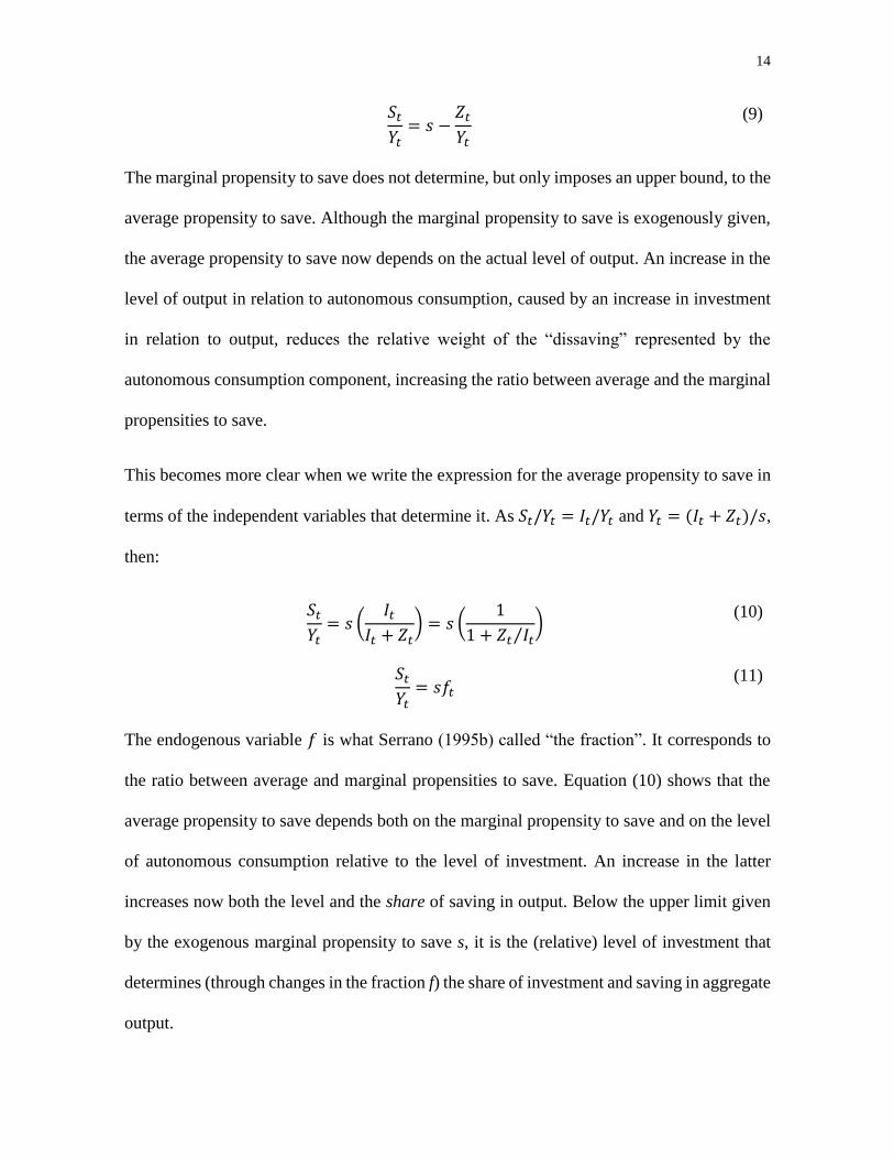
𝑆𝑡

𝑌𝑡= 𝑠 −

𝑍𝑡

𝑌𝑡

(9)

The marginal propensity to save does not determine, but only imposes an upper bound, to the

average propensity to save. Although the marginal propensity to save is exogenously given,

the average propensity to save now depends on the actual level of output. An increase in the

level of output in relation to autonomous consumption, caused by an increase in investment

in relation to output, reduces the relative weight of the “dissaving” represented by the

autonomous consumption component, increasing the ratio between average and the marginal

propensities to save.

This becomes more clear when we write the expression for the average propensity to save in

terms of the independent variables that determine it. As 𝑆𝑡/𝑌𝑡 = 𝐼𝑡/𝑌𝑡 and 𝑌𝑡 = (𝐼𝑡 + 𝑍𝑡)/𝑠,

then:

𝑆𝑡

𝑌𝑡= 𝑠 (

𝐼𝑡𝐼𝑡 + 𝑍𝑡

) = 𝑠 (1

1 + 𝑍𝑡 𝐼𝑡⁄)

(10)

𝑆𝑡

𝑌𝑡= 𝑠𝑓𝑡

(11)

The endogenous variable 𝑓 is what Serrano (1995b) called “the fraction”. It corresponds to

the ratio between average and marginal propensities to save. Equation (10) shows that the

average propensity to save depends both on the marginal propensity to save and on the level

of autonomous consumption relative to the level of investment. An increase in the latter

increases now both the level and the share of saving in output. Below the upper limit given

by the exogenous marginal propensity to save s, it is the (relative) level of investment that

determines (through changes in the fraction f) the share of investment and saving in aggregate

output.

15

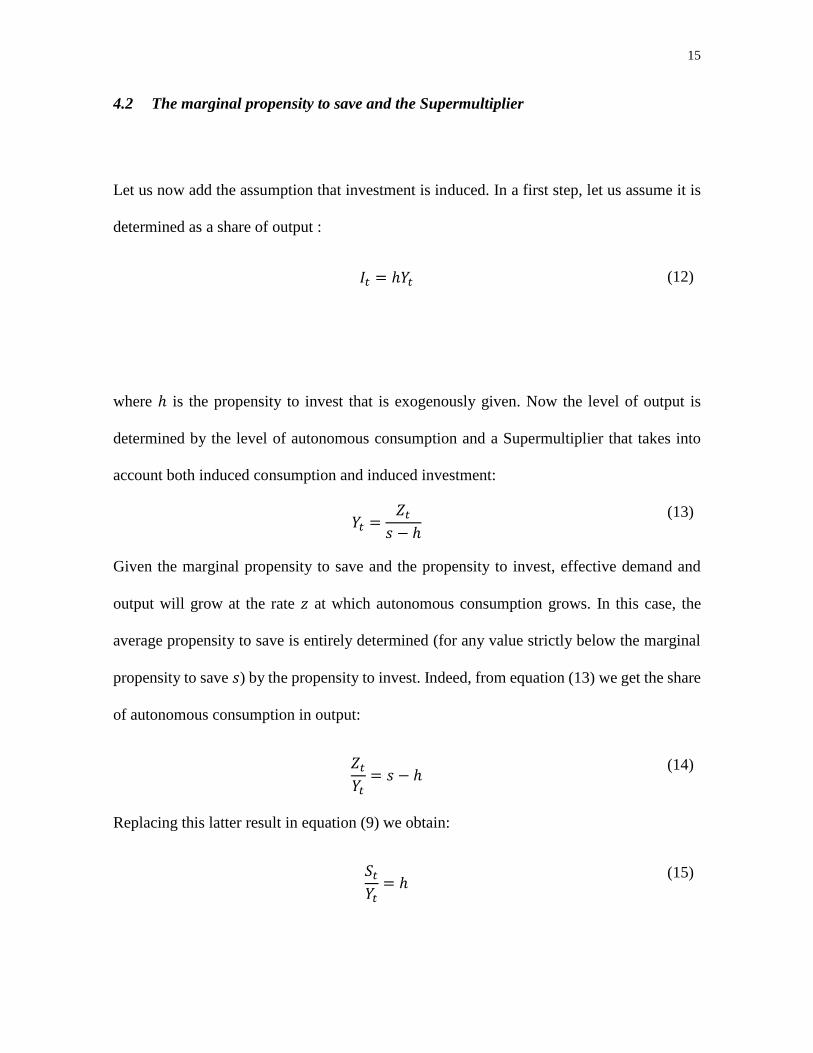
4.2 The marginal propensity to save and the Supermultiplier

Let us now add the assumption that investment is induced. In a first step, let us assume it is

determined as a share of output :

𝐼𝑡 = ℎ𝑌𝑡 (12)

where ℎ is the propensity to invest that is exogenously given. Now the level of output is

determined by the level of autonomous consumption and a Supermultiplier that takes into

account both induced consumption and induced investment:

𝑌𝑡 =𝑍𝑡

𝑠 − ℎ

(13)

Given the marginal propensity to save and the propensity to invest, effective demand and

output will grow at the rate 𝑧 at which autonomous consumption grows. In this case, the

average propensity to save is entirely determined (for any value strictly below the marginal

propensity to save 𝑠) by the propensity to invest. Indeed, from equation (13) we get the share

of autonomous consumption in output:

𝑍𝑡

𝑌𝑡= 𝑠 − ℎ

(14)

Replacing this latter result in equation (9) we obtain:

𝑆𝑡

𝑌𝑡= ℎ

(15)

16

4.3 The Static or fundamental stability of the adjustment of capacity to demand

Our Supermultiplier model allows us to rewrite equation (4) above as:

𝑧 =ℎ

𝑣𝑢

(16)

Due to the presence of autonomous expenditures that do not create capacity and grow at an

exogenous rate 𝑧, the fact that investment is induced in the sense discussed above does not

lead to fundamental or static instability as in Harrod’s model. In fact, contrary to what

happens in the latter l, the autonomous consumption Supermultiplier presented here is

fundamentally or statically stable in Hicksian terms, since the reaction of investors put the

economy in the direction of the equilibrium point. In Harrod’s case, as seen above, if initially

the growth rate of investment happens to be above the warranted rate 𝑠/𝑣, the actual degree

of capacity utilization will be above its planned level and, conversely, if the rate of growth

of investment happens to be lower than the warranted rate this will lead to a situation of

underutilization of capacity. If investment follows the capital stock adjustment principle, the

disequilibrium process drives the economy away from the equilibrium point, because

overutilization (underutilization) leads to a higher (lower) rate of growth of investment and

this will, by its turn, make the actual degree of utilization increase (decrease) even further.13

13 Some authors (but not Harrod) have extended this idea of the warranted rate of growth for the case in which

there are autonomous components in demand (𝑍). In this case the modified warranted rate would be equal to

𝑔𝑤 = (𝑠 − 𝑍/𝑌∗)/𝑣, the ratio between the average propensity to save at a position in which capacity is utilized

at its planned degree and the normal capital-output ratio. This modified warranted rate would measure the

potential rates of growth of capacity saving, and, in general, is not constant over time, as 𝑍/𝑌 could only remain

constant in case the rate of growth of autonomous consumption by chance happened to be equal to the rate of

growth of capacity output. For references and a detailed analysis of this modified warranted rate and the

confusion between this supply side rate of growth with the demand led Sraffian Supermultiplier see Freitas &

Serrano (2015).

17

In the case of the Sraffian Supermultiplier model, growth at Harrod’s warranted rate is still

unstable because that rate only determines an upper limit to feasible demand led rates of

growth. But in this model, where the rate of growth of the trend of demand will be given by

the rate of growth of autonomous expenditures 𝑧, growth at this rate is fundamentally or

statically stable. Starting from a situation in which utilization is equal to its planned degree,

if the rate of growth of investment 𝑔𝐼 happens to be initially above the rate of growth of

autonomous demand 𝑧, the rate of growth of aggregate demand will be lower than the growth

of capacity, which will lead to underutilization of capacity. On the other hand, if the rate of

growth of investment happens to be below the rate of growth of autonomous demand, demand

will grow by more than investment and this will lead to an overutilization of productive

capacity.

If investment is induced according to the capital stock adjustment principle, either directly

by the deviation of the actual degree of utilization from its planned degree, or by the effect

of actually observed growth rates on the expected growth rate of the trend of demand (or

both) this gives the signals in the right direction for the change in investment. In case of

under(over)utilization there will be a tendency for investment to grow by less (more) than

demand, i.e., towards a lower (higher) investment share ℎ, which will tend to make capacity

grow by less (more) than demand.

As an example, let us assume that, starting from a situation in which capacity and demand

are balanced, there is a reduction in the rate of growth 𝑧 of autonomous consumption. This

reduction will provoke a reduction to the same extent of the rate of growth of demand and

output 𝑔 for given values of the marginal propensity to consume and of the investment share.

The actual degree of capacity utilization will be reduced (and now 𝑢 < 1), as initially

18

aggregate demand will start to grow less and only later the rate of growth of productive

capacity and the capital stock will tend to grow at this same lower rate according to equation

(3). The lower growth of capacity will happen when the capacity effect of the lower absolute

rate of growth of investment, for the given propensity to invest, ℎ , materializes. Investment

will grow at the same lower rate of growth as autonomous expenditures, reducing also the

rate of growth of the stock of capital. When the rate of growth of the stock of capital adapts

itself to this lower rate of growth of demand and output, the actual degree of capacity

utilization will stabilize at a level lower than the planned or normal degree, according to

equation (16) above (i.e. 𝑢 = 𝑣𝑧 ℎ⁄ ).

However, it seems to be reasonable to assume that, over time, the investment share ℎ will

itself be reduced to some extent as a response to the underutilization of capacity and/or

reduction of the actual rate of growth of demand. This gradual reduction of the propensity to

invest14 will have two effects. First, it will further reduce the growth of aggregate demand

and output, lowering even more the actual degree of capacity utilization. Nevertheless, later

on, the lower investment share will reduce the rates of growth of the capital stock and

productive capacity. The presence of autonomous consumption demand growing at an

exogenous rate 𝑧 implies that the rate of growth of aggregate demand and output will fall

proportionately less than the rate of growth of investment (for otherwise the investment share

could not have fallen). The ensuing reduction in the rate of growth of capacity and of capital

14 The central idea is that investors attempt to adjust the size of the capital stock to the trend level of demand.

This implies that the investment share will respond to changes in the expected demand trend to situations of

over/underutilization of capacity or to both. There are many forms to represent this process in simple terms in

supermultiplier models. One option is to assume that the investment share reacts linearly to discrepancies

between the actual and the planned degree of capacity utilization, as done in Freitas & Serrano (2015) and

Serrano & Freitas (2017). Here we adopt a different specification in which the investment share reacts linearly

to the revisions on the expected trend rate of growth of demand, as suggested in Cesaratto, Serrano & Stirati

(2003).

19

stock will be equal to the fall in the rate of growth of investment. This means that the actual

degree of capacity utilization will eventually start to rise, because, while aggregate demand

is growing at a slower pace than before, the final reduction of the rate of growth of the capital

stock is even greater (something that would be impossible without the presence of

autonomous consumption).

The same process described above will continue to work as long as the actual degree of

capacity utilization is below the planned degree. It will only stop when the investment share

ℎ has been sufficiently reduced to a level that would allow that, at the planned degree of

capacity utilization, the rate of growth of the capital stock is fully adapted to the lower rate

of growth of autonomous consumption. Obviously, depending on the value of the parameters

defining the intensity of the reaction of investment to demand growth and/or the gap in

capacity utilization, this adjustment process may overshoot and cause a cyclical adjustment.

If the resulting cycle is dampened, this would not cause any problem. But that will depend,

as we shall see below, on the conditions for dynamic, not static, stability.

The same process of adjustment of the propensity to invest will occur symmetrically in the

case of a permanent increase in the rate of growth of autonomous consumption 𝑧. We would

then have an initial overutilization of capacity and, gradual increases in the investment share

ℎ that first would increase further the degree of overutilization. However, the higher

investment share will eventually make the capital stock and the productive capacity grow at

a faster pace than the aggregate demand and output. As a result, the actual degree of capacity

utilization would gradually fall back to its planned degree either monotonically or through

dampened cyclical oscillations, and the level and rate of growth of the productive capacity

20

of the economy will adapt itself to the permanently higher rate of growth of autonomous

demand 𝑧.

The crucial point is that the process of growth led by the expansion of autonomous

consumption is thus fundamentally or statically stable because the reaction of induced

investment to the initial imbalance between capacity and demand has, at some point during

the adjustment disequilibrium process, a greater impact on the rate of growth of productive

capacity than on the rate of growth of demand. Thus, in the case of an initial underutilization

(overutilization) of capacity, the consequent reduction (increase) in the rate of growth of

investment growth in relation to the growth rate of demand and output eventually leads to a

situation in which the rate of growth of the capital stock (and capacity) is lower (higher) than

the rate of growth of demand/output. The operation of the capital stock adjustment principle

combined with the existence of an autonomously growing non-capacity creating expenditure

reverts the initial tendency towards an increasing deviation between actual and planned

degrees of capacity utilization. In this sense, we may say that disequilibrium process in the

Sraffian Supermultiplier model goes in the correct direction.

In the Harrodian model this reaction always causes instability because, without the

autonomous consumption component (𝑍 = 0), the rate of growth of demand always increases

or decreases by the same amount as the rate of growth of capacity (which necessarily comes

later). Given income distribution, the lack of autonomous consumption demand ensures that

no matter how much the levels of investment change, the investment share cannot change

since it is uniquely determined by the marginal propensity to save 𝑠 in the Harrodian model.

In contrast, in the Sraffian Supermultiplier, the average propensity to save is entirely

determined by the propensity to invest decided by firms. If the latter increases (decreases)

21

with overutilization (underutilization) and/or increases (decreases) in the rate of growth of

aggregate demand, the same occurs with the average propensity to save (𝑆/𝑌), that adjusts

itself to the investment share that is required to adjust the level and growth rate of capacity

to that of demand. In equation (11) above, given 𝑠 and 𝑣, changes in the propensity to invest

ℎ modify the “fraction” 𝑓 = [𝐼/(𝐼 + 𝑍)], to the extent that is necessary for the economy to

endogenously generate the saving ratio required by the expansion of aggregate demand,

making the degree of capacity utilization tend to the planned degree (𝑢 = 1). In this sense, if

we were to reinterpret the “warranted rate of growth” as the ratio between average propensity

to save and normal capital-output ratio (see note 14 above), in the Supermultiplier model it

is the “warranted rate” that would adjust itself to the actual rate of growth through changes

in the average (but not the marginal) propensity to save, triggered by induced variations in

the investment share. The upshot is that the “marriage” between the “accelerator” and the

“multiplier” can in principle indeed be consummated, but only if a third element, autonomous

expenditures that do not create capacity, is present.

4.4 Dynamic Stability and the limits to demand led growth

In the discussion of the adjustment of capacity to demand above we have alluded to the idea

of a gradual adjustment of the propensity to invest in relation to discrepancies between the

actual (𝑢) and the planned degree (𝑢 = 1) of capacity utilization. The reason for this is that

the fundamental or static stability of the adjustment of capacity to demand is certainly a

necessary but not a sufficient condition for the viability of a demand led growth regime

described by the the Sraffian Supermultiplier. The partial or gradual adjustment of the

22

investment share is what is required to provide a set of sufficient conditions for the dynamic

stability of the whole process.

If, for instance, given an increase in the growth rate of autonomous consumption 𝑧 and the

consequent increase in the rate of growth of aggregate demand and of the ensuing

overutilization of capacity, the marginal propensity to invest reacts too intensely and

increases too much, it is possible that the whole process of adjustment of capacity to demand

becomes dynamically unstable. This is so, because, although the process is going in the right

direction, its intensity may be excessive if induced investment increases too much. In fact, if

the increase in the investment share is sufficiently large the consequent growth of aggregate

demand may become so high that it may be impossible to increase the supply of output at

such rate. Formally, it is easy to see that if the propensity to invest ℎ when added to the

marginal propensity to consume 𝑐 becomes greater than one, then any positive level of

autonomous consumption demand will induce an infinite total level of aggregate demand,

which is, of course, impossible to meet with increases in output. The dynamic stability of the

model requires that this situation does not occur. This is why the model requires the

additional assumption that the changes of the propensity to invest induced by the changes in

the actual growth rates of demand and/or in the deviations from the planned degree of

utilization should be gradual or partial.

This idea of partial or gradual adjustment can be illustrated by a version of the model in

which the investment share depends only on the technical normal capital-output ratio and the

expected rate of growth of the trend of aggregate demand 𝑔𝑒. The central point is that the

investment share does not depend only on the actual rate of growth 𝑔𝑡−1 observed in the most

recent period (as in the so called “rigid” accelerator) but on the expected trend of demand

23

growth over the life of the new capital equipment. When the actual rate of growth of

aggregate demand 𝑔 changes, the expected trend rate of growth of demand 𝑔𝑒 will be revised,

but only partially and gradually. This is so because firms understand both that demand is

subject to fluctuations that may not be permanent and also because in an economy that uses

fixed capital equipment, the purpose of firms is to adjust capacity to demand over the lifetime

of the equipment and not at each moment in time. This gradual or partial adjustment of

demand expectations is known as the “flexible accelerator” as opposed to the “rigid

accelerator” in which firms try to adapt capacity to demand immediately and treat all changes

in demand as permanent. Thus, gradual adjustment of the propensity to invest can be

represented as follows:

ℎ𝑡 = 𝑣𝑔𝑡𝑒 (17)

𝑔𝑡𝑒 = 𝑔𝑡−1

𝑒 + 𝛽(𝑔𝑡−1 − 𝑔𝑡−1𝑒 ) (18)

where 0 ≤ 𝛽 ≤ 1 is an adjustment parameter in the equation of (adaptive) expectation

formation. Of course, 𝛽 = 0 would mean that the investment share is exogenous, in which

case we would obtain the model analyzed in the last section. On the other hand, 𝛽 = 1 would

represent the case of the “rigid accelerator”. Finally, a positive and small 𝛽 being the more

realistic case of the “flexible accelerator”.

Mathematically (see appendix B below for details), a sufficient condition for the dynamic

stability of the Sraffian Supermultiplier is that the aggregate marginal propensity to spend

both in consumption and investment has to remain lower than one during the adjustment

process, in which the marginal propensity to invest will naturally be changing. In the analysis

of this condition we must take into account the investment share permanently induced or

required by the trend rate of growth of the economy 𝑣𝑧, the marginal change in the investment

24

share induced by the revision of the expected trend of growth 𝑣𝛽 out of equilibrium and the

interaction term involving the two previous terms, 𝑣𝛽𝑧. For the stability condition to be met,

the sum of these components must be lower than the marginal propensity to save 𝑠:15

𝑣𝑧 + 𝑣𝛽 + 𝑣𝛽𝑧 < 𝑠 (19)

From the above condition, we can show that, for a given value of 𝛽, there is a well-defined

upper bound to what can be characterized as a demand led growth regime. This limit shows

that the economy is in a proper demand led regime only if the growth rate of autonomous

demand 𝑧 is not “too high”, namely if:

𝑧 < (𝑠

𝑣− 𝛽)

1

1 + 𝛽

(20)

If condition (19) is met and the Sraffian Supermultiplier is dynamically stable, there will be

a tendency for the investment share to adjust itself to the value required by the trend rate of

growth of demand, which of course will be equal to and determined by the rate of growth of

autonomous consumption 𝑧 (𝑔𝑒 = 𝑔∗ = 𝑧):

ℎ∗ = 𝑣𝑧 (21)

and thus:

𝑌𝑡∗ =

𝑍𝑡

𝑠 − 𝑣𝑧

(22)

15 Existing proofs of the dynamic stability of the Sraffian Supermultiplier by Freitas & Serrano (2015), Pariboni

(2015), Dutt (2015) and Allain (2015) use continuous time and are equivalent to 𝑣𝑧 + 𝑣𝛽 < 𝑠. In discrete time

we see that we have to add the interaction term 𝑣𝛽𝑧 to the marginal propensity to invest. Note also that this

condition shows that the usual stability conditions for static multiplier-accelerator models of business cycles in

which autonomous demand remains constant, namely, 𝑣𝛽 < 𝑠 appear here as a special case of equation (19),

by setting 𝑧 equal to zero.

25

As under these assumptions, the level of productive capacity and the capital stock tends to

adjust itself to the trend levels of demand and output we also have that:

𝑌𝑡∗ =

1

𝑣𝐾𝑡 =

𝑍𝑡

𝑠 − 𝑣𝑧

(23)

Therefore, there is a tendency for the levels of capacity output to follow the evolution of the

trend of effective demand and for the growth rate of demand to be led by the expansion of

the autonomous expenditures that do not create capacity, 𝑍.

The research based on the Sraffian Supermultiplier was set out to determine under which

conditions growth could be unambiguously demand led under exogenous distribution and

with investors driven to adjust capacity to demand. Three such conditions were found to be

required. The first is the existence of autonomous component in demand that does not create

capacity for the private sector of the economy. The second was that investment must be

induced by the capital stock adjustment principle. The third is that in the adjustment of

capacity to demand, the further amount of induced consumption and investment generated

should not be excessive (i.e. infinite). This third condition has two elements. First, one

structural element is that the rate of growth of autonomous demand must be lower than

Harrod’s warranted rate 𝑠/𝑣 as the share of required induced investment to meet the

expansion of autonomous demand 𝑣𝑧 must be permanently lower than the marginal

propensity to save 𝑠, which implies that 𝑧 < 𝑠/𝑣. The second element is due to the fact that

room must be made also for the extra induced investment that is necessary to bring the

economy back to the planned degree of capacity utilization when it deviates from it during

the adjustment process (i.e., 𝑣𝛽). Including this second element (and its interaction with the

26

first one) we get a lower maximum rate of demand led growth, described by equation (20)

above (i.e., we have (𝑠 𝑣⁄ − 𝛽)(1 [1 + 𝛽]⁄ ) < 𝑠 𝑣⁄ for 𝛽 > 0).

Note however that this more stringent condition (20), while sufficient, is not strictly

necessary and could be relaxed to some extent if some of the model parameters were variable.

This relaxation could be accomplished if we assume that the marginal propensity to spend

happens to be higher than one in the vicinity of the position where capacity is fully adjusted

to demand, but then becomes lower than one again when the economy is further away from

that position, generating a limit cycle. There are many possible reason for these type of

assumptions, some reasonable, some quite forced and implausible. Some of these

possibilities will be the subject of further research. But it is important to note that the

structural element of the third condition above related to the fact that the maximum rate of

demand led growth must be lower than Harrod’s own warranted rate16 simply cannot be

relaxed, for it is a necessary condition.

5 FINAL REMARKS

In this paper we have shown that the fundamental instability of Harrod’s warranted rate is

valid under very general conditions. We argued that Harrodian instability is a case of static

instability, in the sense of Hicks (1965) as the adjustment goes in the opposite direction in

relation to the equilibrium position, independently of the magnitude of the reaction parameter

𝛼.17 The upshot of our analysis is that, after all, Harrod’s principle of fundamental (or static)

16 This is the maximum rate of growth proposed initially by Serrano (1995a, 1995b). 17 We may here contrast these results with a recent contribution by Trezzini (2017), where he explicitly argues

that the “the cornerstone of Harrodian instability” (Trezzini (2017), p.2) is the intensity of the reaction of invest

to demand: “the assumption of the elasticity of investment to any divergence between actual and planned

27

instability of his warranted rate should not be seen as a “problem”. Given the fact that the

warranted rate 𝑠/𝑣 is, at best, an upper limit of feasible rates of demand led growth of

capacity output, there is indeed no reason for such a rate of growth to be stable. This is so,

because there is no reason for investors following market signals in a decentralized monetary

capitalist economy to make the economy expand along a path described by Harrod’s

warranted rate. So we do not think it is neither theoretically fruitful nor realistic (given that

we would have had to assume a completely implausible positive reaction of investment to

underutilization) to try to stabilize growth at Harrod’s warranted rate.18 19

This, however, does not imply that the multiplier-accelerator interaction in the analysis of

growing economies is, in general, fundamentally unstable. Quite the contrary, if there is an

autonomous demand component that does not create capacity in the model, as shown by the

Sraffian Supermultiplier, demand led growth at the rate at which this component grows is

fundamentally (or statically) stable. We also argue that the latter result follows from

assumptions about the non-capacity creating expenditures and not from those about the

utilization must be reconsidered. As the concept of Harrodian instability is based on this assumption, it appears

to lose most if not all of its relevance” (Trezzini, 2017, pp. 21-22). As we saw above in section 3 and is

confirmed in appendix A below, Harrod’s instability is fundamental or static precisely because it depends only

on the sign but not on the magnitude of the reaction of investment to demand or to the deviation of capacity

utilization from its planned level. Low reaction coefficients will certainly not prevent the instability of economic

growth at Harrod’s warranted rate. 18 Setterfield (2016) has argued that the canonical Neo-Kaleckian model may avoid Harrodian instability if

investment only reacts to large deviation from the planned degree of utilization. The argument is developed as

if investment is done by a single firm and it is not clear that it could be generalized to a number of different

firms. To us it seems reasonable to think that if only a few firms experience underutilization (or overutilization)

of its capacity large enough to trigger the proper capital stock adjustment principle, then a process of reduction

(increase) in induced investment would quickly drag the degree of capacity utilization of other firms outside

their tolerance bands and joint in the explosive contraction (expansion). In any case, even if aggregate

investment does not react to discrepancies between capacity and demand, it would be growth at the rate

determined by the pace of capital accumulation as given by the Neo-Kaleckian investment function and not

growth at Harrod’s warranted rate, that could be considered stable. 19 It is beyond our purpose to discuss the Cambridge closure which endogenizes the warranted rate by means

of changes in distribution. For a criticism of this closure from the perspective of the Sraffian Supermultiplier

see Serrano(1995b) and Serrano & Freitas (2017).

28

investment function. However, although the adjustment is fundamentally stable, assumptions

on the investment function, in particular that of a gradual or flexible accelerator, are relevant

because, if the accelerator effect is too strong (as measured by a high value for the reaction

parameter 𝛽) the model may nevertheless be dynamically unstable. This does not reduce in

our view the relevance of the Sraffian Supermultiplier model, as we do think that for both

theoretical and empirical reasons, a flexible accelerator moderate reaction of the investment

share to demand is a reasonable assumption.20

Recently, some Neo-Kaleckian authors have used the adjustment mechanism of the Sraffian

Supermultiplier, with autonomous demand allowing the endogenous adjustment of the

investment share to its required value through changes in ratio between the average and

marginal propensity to save, in order to tackle what they call the “Harrodian instability” of

their demand led growth models. These authors are correct in considering that Neo-Kaleckian

models without autonomous non-capacity creating demand are subject to Harrodian

instability, if investment is allowed to follow consistently the capital stock adjustment

principle. They are also correct in seeing that, in models that do include such an autonomous

demand component, the equilibrium can be dynamically stable if the reaction of investment

to demand is not excessive. The problem of the traditional Neo-Kaleckian models without

non-capacity creating autonomous demand is indeed one of Harrod’s fundamental or static

instability. That is why instability does not depend on the value of the parameters. However,

in the case of their Supermultiplier type of models, the notion of Harrod’s fundamental

instability does not really apply. These models can of course also be unstable if the reaction

20 For empirical evidence supporting the Sraffian Supermultiplier see Girardi & Pariboni (2016) and Avancini,

D., Freitas, F. & Braga, J. (2016). More generally, as shown by Hillinger (1992), among many others, there is

a lot of evidence in favor of dampened “flexible” accelerator business investment cycles.

29

of investment is too strong. Nevertheless, if this happens to be the case, it is a matter of

dynamic, not static or fundamental instability. Moreover, as the dynamic stability condition

for the Supermultiplier is directly related to the requirement of the marginal propensity to

spend to be lower than one during the adjustment process, it is clearly a variant of what the

Neo-Kaleckians call “Keynesian instability” (marginal propensity to invest lower than

marginal propensity to save) instead of “Harrodian instability”. We thus think that the notion

of Harrodian instability should be used only in demand led models without autonomous

demand, where the investment share is determined by the marginal propensity to save. It

should not be applied to Supermultiplier models (whether of Sraffian or Neo-Kaleckian

inspiration) to avoid confusing the necessary conditions of fundamental or static stability

with those of the sufficient conditions of dynamic stability.21 22

We thus hope that our new results and the clarification of these issues concerning static and

dynamic stability in both the Harrod and the Sraffian Supermultiplier models will prove to

be useful to the small but steadily growing Sraffian,23 and now increasingly Neo-Kaleckian

too (Lavoie (2016)), literature on the Supermultiplier.

21 For a detailed analysis of this point in relation to these new Neo-Kaleckian growth models see Fagundes &

Freitas (2017). 22 Franke (2017) has recently argued that even a dynamically stable adjustment of capacity to demand via a

flexible accelerator Supermultiplier can be made unstable, if combined with another adjustment process such

as those used to stabilize growth at Harrod’s warranted rate. But we know (see footnote 12 above) that the latter

adjustment process implies that the rate of growth of investment increases when the degree of utilization falls

below the planned level (and decreases with overutilization). Thus in the context of the Sraffian Supermultiplier

if this added effect is sufficiently strong it could counteract the capital stock adjustment principle and would be

equivalent to assuming a negative value for the reaction of investment to demand parameter 𝛽. We do not find

such assumptions plausible, but, in any case, it should be noted that under such extreme circumstances the

Sraffian Supermultiplier would become statically unstable as the adjustment process would be clearly going in

the wrong direction. 23 Dejuán (2016) uses his variant of the Sraffian Supermultiplier model that has autonomous component that

does not create capacity and thus, as we have seen above does not suffer from Harrod’s fundamental or static

instability. He does make further assumptions that firms immediately adjust the marginal propensity to

investment to the trend rate of growth of autonomous demand and perform temporary levels of investment to

deal with initial under or overutilization of capacity. These latter “ancilliary” investments, according to him,

have no further accelerator effects as they do not affect the expected trend rate of growth. The author is correct

30

References

Ackley, G. (1963) “Un modello econometrico dello sviluppo italiano nel dopoguerra”,

SVIMEZ, Giuffré, Roma.

Avancini, D., Freitas, F., Braga, J. (2016): “Investment and Demand Led Growth: a study of

the Brazilian case based on the Sraffian Supermultiplier Model [Investimento e

Crescimento Liderado Pela Demanda: um estudo para o caso brasileiro com base no

modelo do Supermultiplicador Sraffiano]”, Annals of the XLIII Meeting of the

Brazilian Association of Graduate Programs in Economics (ANPEC) (in Portuguese),

Florianópolis, Brazil, 2016.

Besomi, D. (2001): “Harrod's dynamics and the theory of growth: the story of a mistaken

attribution” Cambridge Journal of Economics, 25 (1), pp. 79–96, DOI:

10.1093/cje/25.1.79.

Cesaratto, S., Serrano, F., Stirati, A. (2003): “Technical Change, Effective Demand and

Employment”. Review of Political Economy, 15 (1), pp. 33-52.

in attributing the strong (dynamic) stability of his own model to these (in our view unrealistic) assumptions that

firms know how to distinguish clearly permanent from temporary changes in demand and also know that the

trend of the economy depends on the growth of autonomous demand component. Moreover, he also argues that:

“[t]he absence of proper autonomous demand in Harrod’s model hindered the structural way out. But even in

his simple model, stability would prevail if it were not for the bizarre reaction function bestowed on investors”

that “links investment both to permanent and transient demand;” (DeJuán, 2016, p. 22). Here he claims that his

assumptions on the ability of firms to distinguish between permanent and transient changes in demand would

be sufficient to ensure that “stability would prevail” in Harrod model without autonomous demand. But what

would “stable”, and in the mere sense of being constant over time, would be the actual rate of growth of

investment, which would not change given the assumed inelasticity of demand expectations. As he readily

admits, this actual rate of growth would be different from Harrod’s warranted rate and the actual degree of

utilization correspondingly permanently different from the planned degree. Therefore, DeJuán (2016) does not

really deny that growth at Harrod’s warranted rate is fundamentally unstable, if investment is allowed to respond

to demand or to the deviation of capacity utilization from its planned degree (and in fact amounts to the same

result obtained by Setterfield (2016)).

31

Cesaratto (2016): “Lo “Studio Svimez” di Garegnani del 1962 – Note preliminari”, mimeo

(in Italian), Universitá di Siena.

DeJuán, Ó. (2016): “Hidden links in the warranted rate of growth: the Supermultiplier way

out”, European Journal of History of Economic Thought, DOI:

10.1080/09672567.2016.1186201.

Dutt, A. (2015): “Autonomous demand growth, distribution and growth”, mimeo, University

of Notre Dame.

Fagundes, L., Freitas, F. (2017) “The Role of Autonomous Non-Capacity Creating

Expenditures in Recent Kaleckian Growth Models: An Assessment from the

Perspective of the Sraffian Supermultiplier Model”, mimeo, Institute of Economics of

the Federal University of Rio de Janeiro.

Fiebiger B., Lavoie, M. (2017): “Trend and Business Cycles with External Markets?: Non-

Capacity Generating Semi-Autonomous Expenditures and Effective Demand”,

Metroeconomica, forthcoming.

Franke, R. (2017): “On Harrodian Instability: Two Stabilizing Mechanisms May be Jointly

Destabilizing”, mimeo, Kiel University.

Freitas, F., Serrano, F. (2015): “Growth Rate and Level Effects, the Adjustment of Capacity

to Demand and the Sraffian Supermultiplier”, Review of Political Economy, 27 (3), pp.

258–81, DOI: 10.1080/09538259.2015.1067360.

Garegnani, P. (1962): Il problema della domanda effettiva nello sviluppo economico italiano,

Rome, SVIMEZ.

Garegnani (2015): “The Problem of Effective Demand in Italian Economic Development:

On the Factors that Determine the Volume of Investment”, Review of Political

Economy, 27 (2), pp. 111-33, DOI: 10.1080/09538259.2015.1026096.

32

Girardi, D., Pariboni, R. (2016): “Long-run Effective Demand in the US Economy: An

Empirical Test of the Sraffian Supermultiplier Model”, Review of Political Economy,

28 (4), pp. 523-54, DOI: 10.1080/09538259.2016.1209893.

Harrod, R. (1939): “An Essay in Dynamic Theory”, The Economic Journal, 49 (193), pp. 14-

33

Harrod, R. (1948): Towards a Dynamic Economics, Macmillan, London.

Harrod, R. (1973): Economic Dynamics, Macmillan, London.

Hicks, J. (1950): A Contribution to the Theory of the Trade Cycle, Clarendon, Oxford.

Hicks, J. (1965): Capital and Growth, Oxford University Press, Oxford.

Hillinger, C. (Ed.) (1992): Cyclical Growth in Market and Planned Economies, Clarendon

Press, Oxford.

Kalecki, M. (1962): “Observations on the Theory of Growth”, Economic Journal, 72 (285),

pp. 134-53.

Kalecki, M. (1967/1991): “The Problem of Effective Demand with Tugan-Baranovski and

Rosa Luxemburg”, In Osiatinyński, J. (Ed.) Collected Works of Michał Kalecki

Volume II, Clarendon Press, Oxford.

Kalecki, M. (1968/1991): “The Marxian equations of reproduction and modern economics”,

In Osiatinyński, J. (Ed.) Collected Works of Michał Kalecki Volume II, Clarendon

Press, Oxford.

Lavoie, M. (2016): “Convergence Towards the Normal Rate of Capacity Utilization in Neo-

Kaleckian Models: The Role of Non-Capacity Creating Autonomous Expenditures”,

Metroeconomica, 67 (1), pp. 172-201.

33

Pariboni, R. (2015): Autonomous Demand and Capital Accumulation: Three Essays on

Heterodox Growth Theory, unpublished Ph.D. Dissertation, Dip. Economia Politica e

Estatistica, University of Siena.

Palumbo, A., Trezzini, A. (2016) “A historical analysis of the debate on capacity adjustment

in the ‘modern classical approach’: dealing with complexity in the theory of growth”,

ESHET 2016 conference, Paris.

Serrano, F. (1995a): “Long Period Effective Demand and the Sraffian Supermultiplier”,

Contributions to Political Economy, 14, pp. 67-90.

Serrano, F. (1995b): The Sraffian Supermultiplier, unpublished Ph.D Dissertation,

Cambridge University, Cambridge.

Serrano, F. (2011): “Stability in Classical and Neoclassical theories”, in R. Ciccone, C.

Gehrke, and G. Mongiovi (Eds.), Sraffa and Modern Economics, Routledge, London

and New York.

Serrano, F, Freitas, F. (2017): “The Sraffian Supermultiplier as an Alternative Closure for

Heterodox Growth Theory”, European Journal of Economics and Economic Policy:

Intervention, 14 (1), pp. 70-91, DOI: 10.4337/ejeep.2017.01.06.

Setterfield, M. (2016): “Long-run variation in capacity utilization in the presence of a fixed

normal rate”, mimeo, New School University, 2016.

Trezzini, A. (2017): “Harrodian Instability: a Misleading Concept”, Centro Sraffa Working

Papers, n. 24, 2017.

Trezzini, A., Palumbo, A. (2016): “The theory of output in the modern classical approach:

main principles and controversial issues”, Review of Keynesian Economics, 4 (4), pp.

503-22, DOI: 10.4337/roke.2016.04.09.

34

APPENDIX A: On the Fundamental or Static Instability of Growth at Harrod’s

Warranted Rate

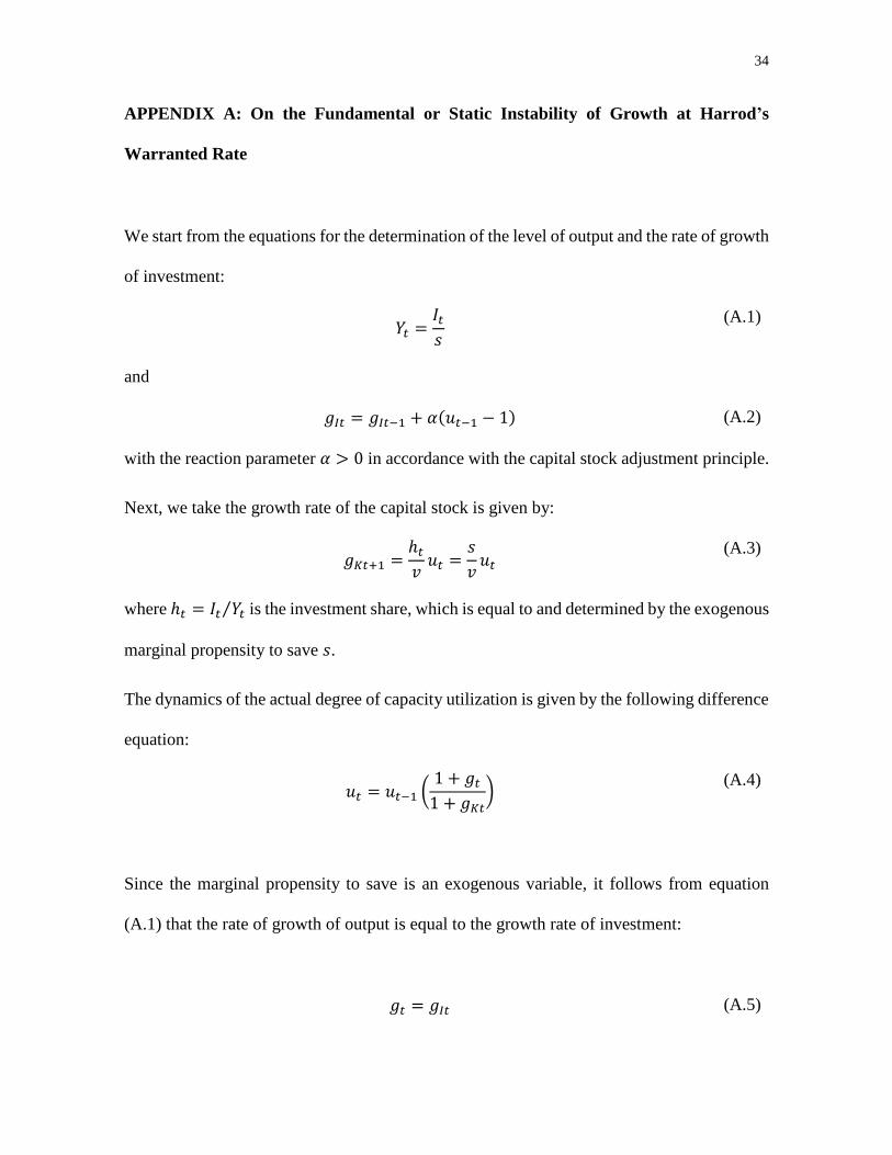
We start from the equations for the determination of the level of output and the rate of growth

of investment:

𝑌𝑡 =𝐼𝑡𝑠

(A.1)

and

𝑔𝐼𝑡 = 𝑔𝐼𝑡−1 + 𝛼(𝑢𝑡−1 − 1) (A.2)

with the reaction parameter 𝛼 > 0 in accordance with the capital stock adjustment principle.

Next, we take the growth rate of the capital stock is given by:

𝑔𝐾𝑡+1 =ℎ𝑡

𝑣𝑢𝑡 =

𝑠

𝑣𝑢𝑡

(A.3)

where ℎ𝑡 = 𝐼𝑡 𝑌𝑡⁄ is the investment share, which is equal to and determined by the exogenous

marginal propensity to save 𝑠.

The dynamics of the actual degree of capacity utilization is given by the following difference

equation:

𝑢𝑡 = 𝑢𝑡−1 (1 + 𝑔𝑡

1 + 𝑔𝐾𝑡)

(A.4)

Since the marginal propensity to save is an exogenous variable, it follows from equation

(A.1) that the rate of growth of output is equal to the growth rate of investment:

𝑔𝑡 = 𝑔𝐼𝑡 (A.5)

35

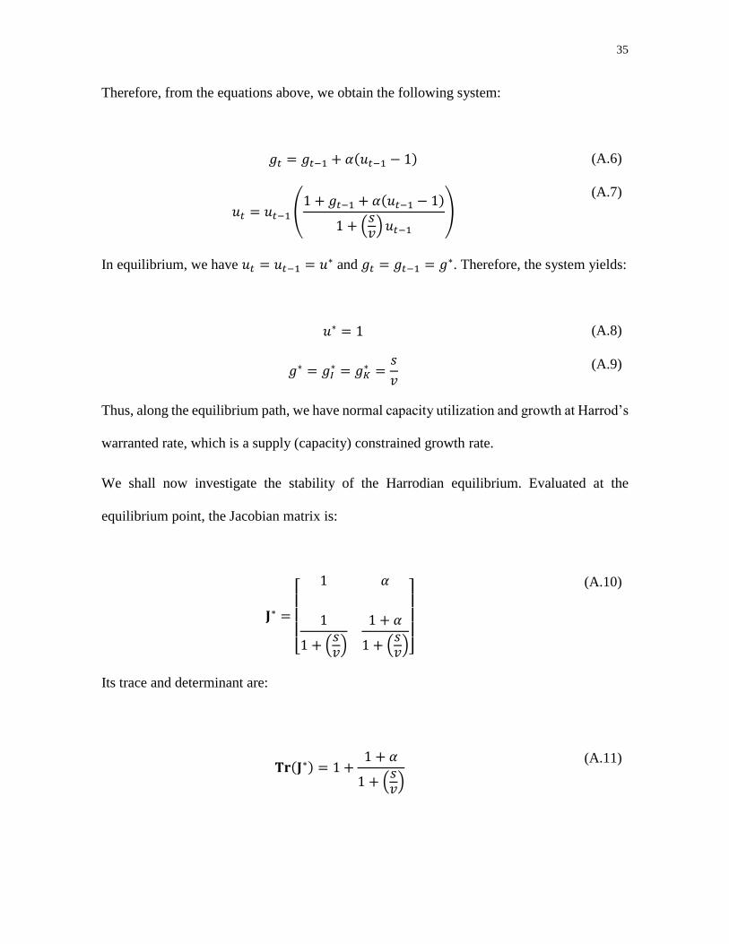
Therefore, from the equations above, we obtain the following system:

𝑔𝑡 = 𝑔𝑡−1 + 𝛼(𝑢𝑡−1 − 1) (A.6)

𝑢𝑡 = 𝑢𝑡−1 (1 + 𝑔𝑡−1 + 𝛼(𝑢𝑡−1 − 1)

1 + (𝑠𝑣)𝑢𝑡−1

)

(A.7)

In equilibrium, we have 𝑢𝑡 = 𝑢𝑡−1 = 𝑢∗ and 𝑔𝑡 = 𝑔𝑡−1 = 𝑔∗. Therefore, the system yields:

𝑢∗ = 1 (A.8)

𝑔∗ = 𝑔𝐼∗ = 𝑔𝐾

∗ =𝑠

𝑣 (A.9)

Thus, along the equilibrium path, we have normal capacity utilization and growth at Harrod’s

warranted rate, which is a supply (capacity) constrained growth rate.

We shall now investigate the stability of the Harrodian equilibrium. Evaluated at the

equilibrium point, the Jacobian matrix is:

𝐉∗ =

[

1 𝛼

1

1 + (𝑠𝑣)

1 + 𝛼

1 + (𝑠𝑣)]

(A.10)

Its trace and determinant are:

𝐓𝐫(𝐉∗) = 1 +1 + 𝛼

1 + (𝑠𝑣)

(A.11)

36

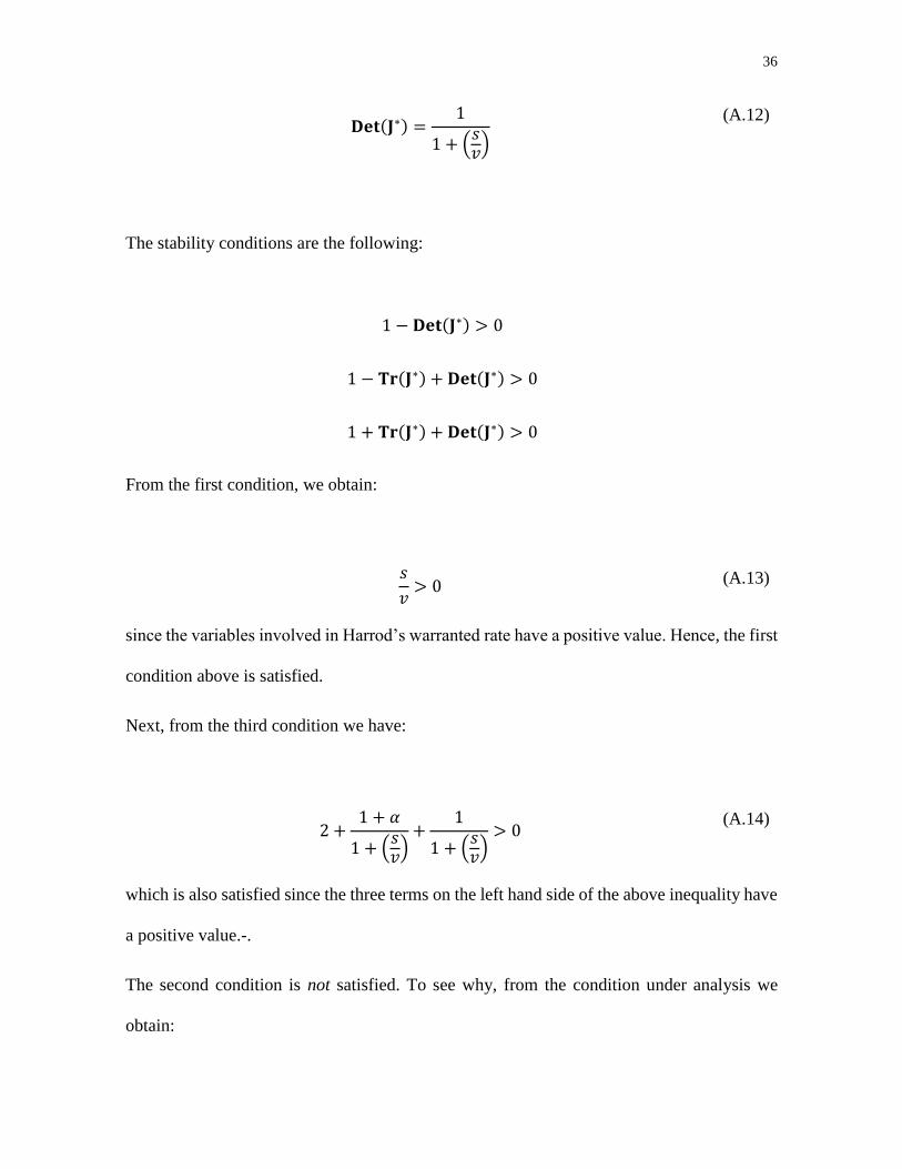
𝐃𝐞𝐭(𝐉∗) =1

1 + (𝑠𝑣)

(A.12)

The stability conditions are the following:

1 − 𝐃𝐞𝐭(𝐉∗) > 0

1 − 𝐓𝐫(𝐉∗) + 𝐃𝐞𝐭(𝐉∗) > 0

1 + 𝐓𝐫(𝐉∗) + 𝐃𝐞𝐭(𝐉∗) > 0

From the first condition, we obtain:

𝑠

𝑣> 0

(A.13)

since the variables involved in Harrod’s warranted rate have a positive value. Hence, the first

condition above is satisfied.

Next, from the third condition we have:

2 +1 + 𝛼

1 + (𝑠𝑣)

+1

1 + (𝑠𝑣)

> 0 (A.14)

which is also satisfied since the three terms on the left hand side of the above inequality have

a positive value.-.

The second condition is not satisfied. To see why, from the condition under analysis we

obtain:

37

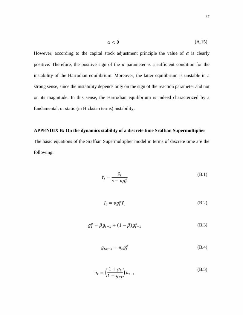
𝛼 < 0 (A.15)

However, according to the capital stock adjustment principle the value of 𝛼 is clearly

positive. Therefore, the positive sign of the 𝛼 parameter is a sufficient condition for the

instability of the Harrodian equilibrium. Moreover, the latter equilibrium is unstable in a

strong sense, since the instability depends only on the sign of the reaction parameter and not

on its magnitude. In this sense, the Harrodian equilibrium is indeed characterized by a

fundamental, or static (in Hicksian terms) instability.

APPENDIX B: On the dynamics stability of a discrete time Sraffian Supermultiplier

The basic equations of the Sraffian Supermultiplier model in terms of discrete time are the

following:

𝑌𝑡 =𝑍𝑡

𝑠 − 𝑣𝑔𝑡𝑒

(B.1)

𝐼𝑡 = 𝑣𝑔𝑡𝑒𝑌𝑡 (B.2)

𝑔𝑡𝑒 = 𝛽𝑔𝑡−1 + (1 − 𝛽)𝑔𝑡−1

𝑒 (B.3)

𝑔𝐾𝑡+1 = 𝑢𝑡𝑔𝑡𝑒 (B.4)

𝑢𝑡 = (1 + 𝑔𝑡

1 + 𝑔𝐾𝑡) 𝑢𝑡−1

(B.5)

38

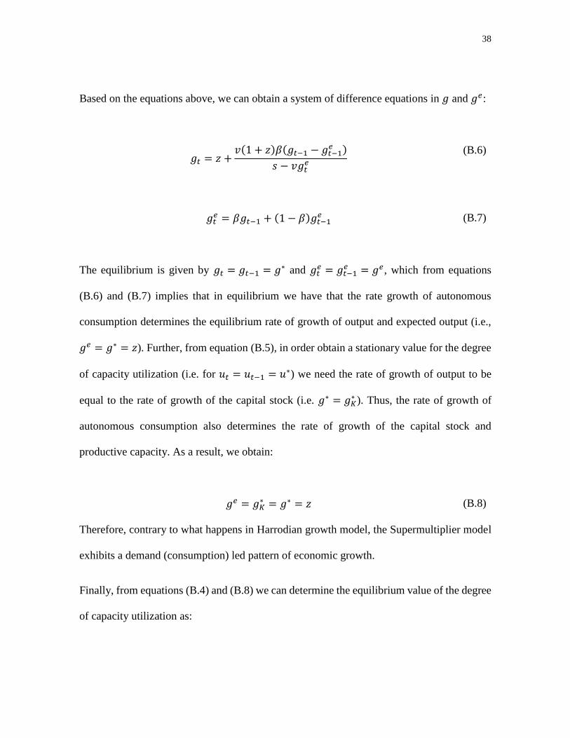
Based on the equations above, we can obtain a system of difference equations in 𝑔 and 𝑔𝑒:

𝑔𝑡 = 𝑧 +𝑣(1 + 𝑧)𝛽(𝑔𝑡−1 − 𝑔𝑡−1

𝑒 )

𝑠 − 𝑣𝑔𝑡𝑒

(B.6)

𝑔𝑡𝑒 = 𝛽𝑔𝑡−1 + (1 − 𝛽)𝑔𝑡−1

𝑒 (B.7)

The equilibrium is given by 𝑔𝑡 = 𝑔𝑡−1 = 𝑔∗ and 𝑔𝑡𝑒 = 𝑔𝑡−1

𝑒 = 𝑔𝑒, which from equations

(B.6) and (B.7) implies that in equilibrium we have that the rate growth of autonomous

consumption determines the equilibrium rate of growth of output and expected output (i.e.,

𝑔𝑒 = 𝑔∗ = 𝑧). Further, from equation (B.5), in order obtain a stationary value for the degree

of capacity utilization (i.e. for 𝑢𝑡 = 𝑢𝑡−1 = 𝑢∗) we need the rate of growth of output to be

equal to the rate of growth of the capital stock (i.e. 𝑔∗ = 𝑔𝐾∗ ). Thus, the rate of growth of

autonomous consumption also determines the rate of growth of the capital stock and

productive capacity. As a result, we obtain:

𝑔𝑒 = 𝑔𝐾∗ = 𝑔∗ = 𝑧 (B.8)

Therefore, contrary to what happens in Harrodian growth model, the Supermultiplier model

exhibits a demand (consumption) led pattern of economic growth.

Finally, from equations (B.4) and (B.8) we can determine the equilibrium value of the degree

of capacity utilization as:

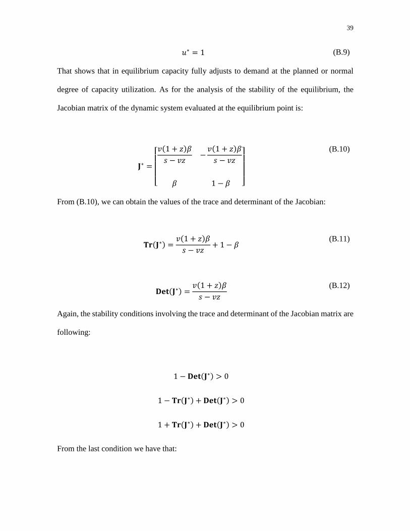
39

𝑢∗ = 1 (B.9)

That shows that in equilibrium capacity fully adjusts to demand at the planned or normal

degree of capacity utilization. As for the analysis of the stability of the equilibrium, the

Jacobian matrix of the dynamic system evaluated at the equilibrium point is:

𝐉∗ =

[ 𝑣(1 + 𝑧)𝛽

𝑠 − 𝑣𝑧−

𝑣(1 + 𝑧)𝛽

𝑠 − 𝑣𝑧

𝛽 1 − 𝛽 ]

(B.10)

From (B.10), we can obtain the values of the trace and determinant of the Jacobian:

𝐓𝐫(𝐉∗) =𝑣(1 + 𝑧)𝛽

𝑠 − 𝑣𝑧+ 1 − 𝛽

(B.11)

𝐃𝐞𝐭(𝐉∗) =𝑣(1 + 𝑧)𝛽

𝑠 − 𝑣𝑧

(B.12)

Again, the stability conditions involving the trace and determinant of the Jacobian matrix are

following:

1 − 𝐃𝐞𝐭(𝐉∗) > 0

1 − 𝐓𝐫(𝐉∗) + 𝐃𝐞𝐭(𝐉∗) > 0

1 + 𝐓𝐫(𝐉∗) + 𝐃𝐞𝐭(𝐉∗) > 0

From the last condition we have that:

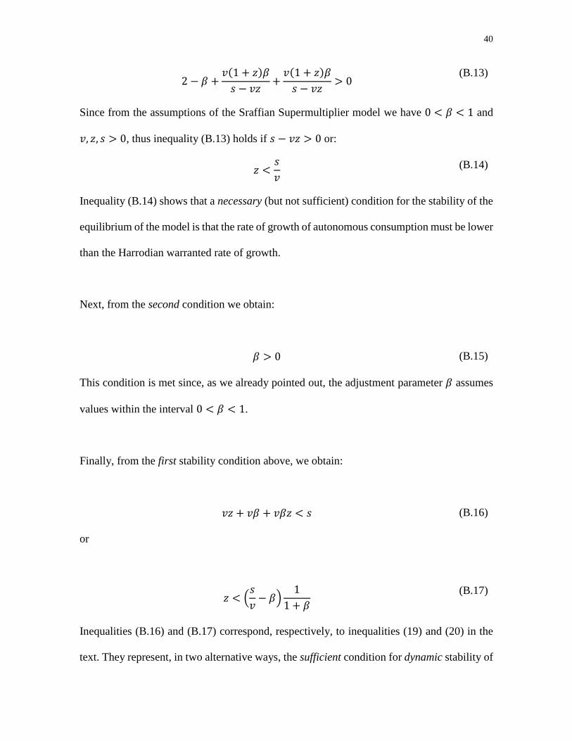
40

2 − 𝛽 +𝑣(1 + 𝑧)𝛽

𝑠 − 𝑣𝑧+

𝑣(1 + 𝑧)𝛽

𝑠 − 𝑣𝑧> 0

(B.13)

Since from the assumptions of the Sraffian Supermultiplier model we have 0 < 𝛽 < 1 and

𝑣, 𝑧, 𝑠 > 0, thus inequality (B.13) holds if 𝑠 − 𝑣𝑧 > 0 or:

𝑧 <𝑠

𝑣

(B.14)

Inequality (B.14) shows that a necessary (but not sufficient) condition for the stability of the

equilibrium of the model is that the rate of growth of autonomous consumption must be lower

than the Harrodian warranted rate of growth.

Next, from the second condition we obtain:

𝛽 > 0 (B.15)

This condition is met since, as we already pointed out, the adjustment parameter 𝛽 assumes

values within the interval 0 < 𝛽 < 1.

Finally, from the first stability condition above, we obtain:

𝑣𝑧 + 𝑣𝛽 + 𝑣𝛽𝑧 < 𝑠 (B.16)

or

𝑧 < (𝑠

𝑣− 𝛽)

1

1 + 𝛽

(B.17)

Inequalities (B.16) and (B.17) correspond, respectively, to inequalities (19) and (20) in the

text. They represent, in two alternative ways, the sufficient condition for dynamic stability of

41

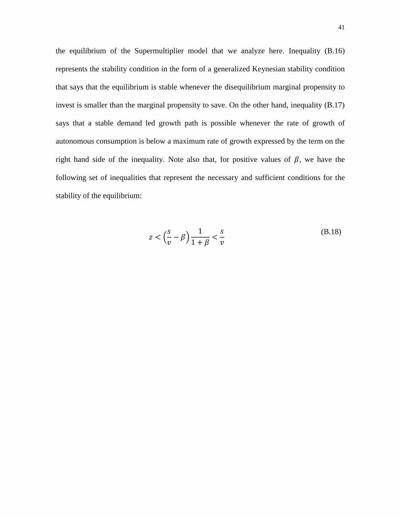
the equilibrium of the Supermultiplier model that we analyze here. Inequality (B.16)

represents the stability condition in the form of a generalized Keynesian stability condition

that says that the equilibrium is stable whenever the disequilibrium marginal propensity to

invest is smaller than the marginal propensity to save. On the other hand, inequality (B.17)

says that a stable demand led growth path is possible whenever the rate of growth of

autonomous consumption is below a maximum rate of growth expressed by the term on the

right hand side of the inequality. Note also that, for positive values of 𝛽, we have the

following set of inequalities that represent the necessary and sufficient conditions for the

stability of the equilibrium:

𝑧 < (𝑠

𝑣− 𝛽)

1

1 + 𝛽<

𝑠

𝑣

(B.18)