The Traveling Salesman Problem in Theory & Practice Lecture 9: Optimization 101, or “How I spent...

The Traveling Salesman Problem in Theory & Practice

Lecture 9: Optimization 101, or“How I spent my Spring Break”

25 March 2014

David S. Johnson

[email protected]://davidsjohnson.net

Seeley Mudd 523, Tuesdays and Fridays

mailto:[email protected]

http://davidsjohnson.net/

http://davidsjohnson.net/

Outline

1. Elementary Exhaustive Search

2. The Value of Pruning

3. More General Branch-and-Bound

4. Student Presentation

Jinyu Xie, on “The Complexity of Facets”

Credits

• J. L. Bentley, “Faster and faster and faster yet,” UNIX Review 15 (1997), 59-67.

• D. L. Applegate, W. J. Cook, S. Dash, A Practical Guide to Discrete Optimization (book in preparation).

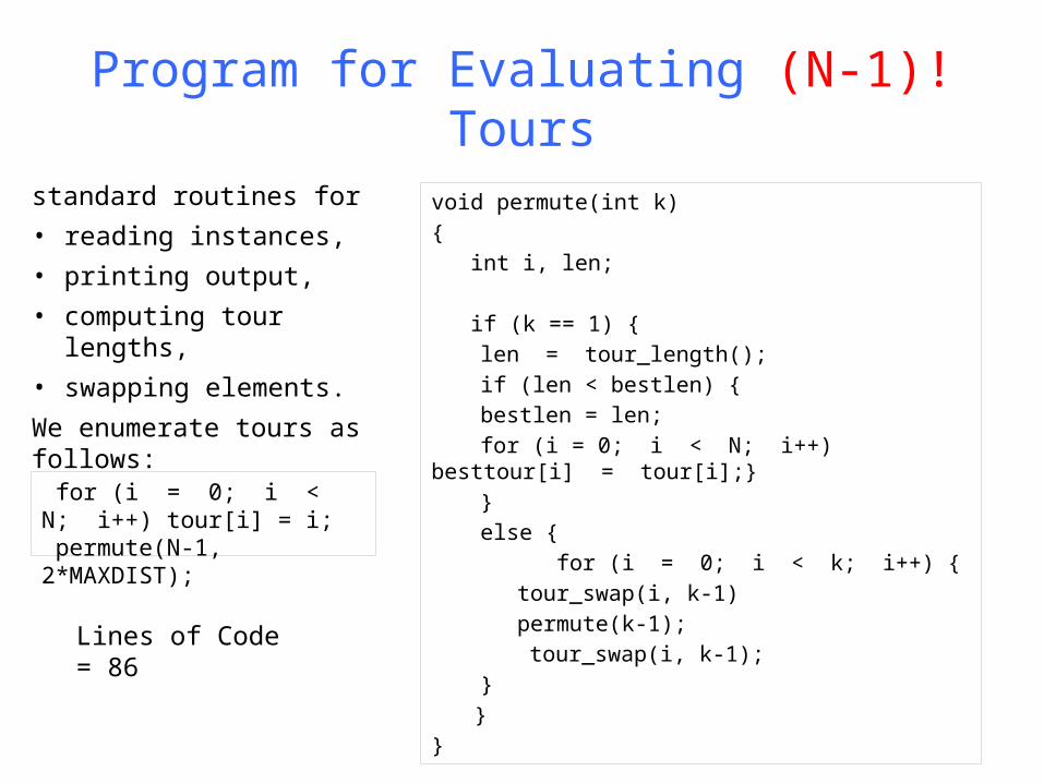
Program for Evaluating (N-1)! Tours

for (i = 0; i < N; i++) tour[i] = i; permute(N-1, 2*MAXDIST);

void permute(int k){ int i, len;

if (k == 1) {len = tour_length();if (len < bestlen) {

bestlen = len;for (i = 0; i < N; i++) besttour[i] =

tour[i];}}else {

for (i = 0; i < k; i++) {tour_swap(i, k-1)permute(k-1);

tour_swap(i, k-1);}

}}

standard routines for

• reading instances,

• printing output,

• computing tour lengths,

• swapping elements.

We enumerate tours as follows:

Lines of Code = 86

Results for Basic Program

Methodology:1. Construct lower triangular distance matrix M for a 100-city

random Euclidean instance.2. Instance IN consists of the first N rows of M.

Advantages:• Somewhat better correlation between results for different N

so running time growth rates are less noisy.• Fewer instances to keep track of.

Disadvantages:• Results may be too dependent on M, so should try different

M’s

Results for Basic Program

N 10 11 12 13 14 15

(N-1)! 362,880 3,628,800 39,916,800

4.8 x 108 6.2 x 109 8.7 x 1010

Seconds 0.02 0.30 2.80 42.1 624 9,353

-O2 Secs 0.00 0.09 1.08 13.5 188 2,970

Suggestions for Speedups?

Compiler Optimization: cc –O2 exhaust.c

Lines of Code, still = 86

(Running times on 3.6 Ghz Core i7 processors in an iMac with 32 Gb RAM)

Next Speedup

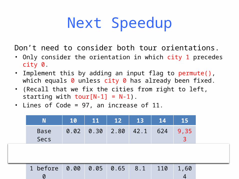
Don’t need to consider both tour orientations.• Only consider the orientation in which city 1 precedes city 0.• Implement this by adding an input flag to permute(), which

equals 0 unless city 0 has already been fixed.• (Recall that we fix the cities from right to left, starting with

tour[N-1] = N-1).• Lines of Code = 97, an increase of 11.

N 10 11 12 13 14 15Base Secs 0.02 0.30 2.80 42.1 624 9,353-O2 Secs 0.00 0.09 1.08 13.5 188 2,970

1 before 0 0.00 0.05 0.65 8.1 110 1,604

Next SpeedupMore efficient distance calculations

void permute(int k){ int i, len;

if (k == 1) {len = tour_length();if (len < bestlen) {

bestlen = len;for (i = 0; i < N; i++) besttour[i]

= tour[i];}}else {

for (i = 0; i < k; i++) {tour_swap(i, k-1)permute(k-1);

tour_swap(i, k-1);}

}}

void permute(int k, int tourlen){ int i, len;

if (k == 1) {tourlen += dist(tour[0],tour[1]) + dist(tour[ncount-

1],tour[0]);if (tourlen < bestlen) {

bestlen = tourlen;for (i = 0; i < N; i++) besttour[i] =

tour[i];}}else {

for (i = 0; i < k; i++) {tour_swap(i, k-1)permute(k-1,

tourlen+dist(tour[k-1],tour[k])); tour_swap(i, k-1);

}}

}

if (tourlen >= bestlen) return;

O(N) factor of improvement – probably worth one additional city.

More valuable idea: Prune!

Lines of code increases from 97 to 99

Results

N 15 16 17 18 19 20 211 before 0 1604 -- -- -- -- -- --

Tourlen 0.50 1.25 3.81 40.3 280 824 4560

Next Speeduptourlen only includes the costs of edges linking the city in slot k through the city in slot N-1.

We would get more effective pruning if we could take into account the edges linking the cities that haven’t yet been fixed.

More precisely we could use a lower bound on the minimum length path involving these cities and linking the city in slot k to city N-1.

An obvious first choice is the length of a minimum spanning tree connecting all these cities.





tour[i];}}else {



}}

}

if (tourlen >= bestlen) return;if (tourlen >= bestlen + mst(k+1)) return;

Lines of code increases from 99 to 134

Results

N 20 21 22 23 24 25 26 27 28 29 30 31Tourlen 824 4560 -- -- -- -- -- -- -- -- -- --

mst 0.15 0.20 0.54 1.44 0.76 2.79 29.5 14.0 17.1 12.3 103.5 84.1

N 32 33 34 35 36 37 38 39 40 41 42 43mst 29.3 43.2 84.6 157 290 232 824 316 225 987 2297 5866

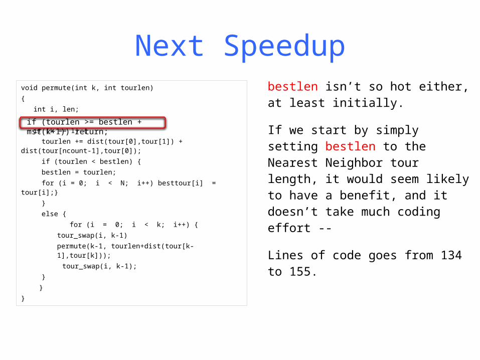
Next Speedupbestlen isn’t so hot either, at least initially.

If we start by simply setting bestlen to the Nearest Neighbor tour length, it would seem likely to have a benefit, and it doesn’t take much coding effort --

Lines of code goes from 134 to 155.





tour[i];}}else {



}}

}

if (tourlen >= bestlen + mst(k+1)) return;

Results

N 32 33 34 35 36 37 38 39 40 41 42 43mst 29.3 43.2 84.6 157 290 232 824 316 225 987 2297 5866

nn 2.9 8.0 24.6 1.3 4.3 4.9 26.8 101 55 407 1357 3653

Next Speedup• As we know from our earlier discussions of tour-construction

heuristics, Nearest Neighbor is a pretty lousy bound, typically 24% above optimal for random Euclidean instances.

• Question: How can we get a better bound cheaply?

• Answer: Guess low – say at (3/4)NN.

– The algorithm will presumably run faster if our initial value of bestlen is less than the optimal tour length.

– If no solution is found, we can rerun the algorithm with an incrementally increased initial value for bestlen, say 5% above the previous value.

– When our initial value eventually exceeds optimal, it will not exceed it by more than 5% (much better than 24%).

– Lines of code increases from 155 to 165.

Results

N 37 38 39 40 41 42 43 44 45 46 47 48nn 232 824 316 225 987 2297 5866 -- -- -- -- --

Iterative 19 71 12 15 33 121 149 2223 756 684 3185 4304

Next Speedup

• A large amount of our time goes into computing MST’s, and much of it may be repeated for different permutations of the same set of cities.

• Could we save time by hashing the results so as to avoid this duplication?

• How would that work?

Set Hashing• Start by creating random unsigned ints hashkey[i], 0 ≤ i < N.

• Create an initial empty hashtable MstTable, say of size hashsize = 524288 = 219. (We will double the size of MstTable whenever half of its entries become full.)

• The hash value hval(C) for a set C of cities is obtained by computing the exclusive-or of the |C| values {hashkey[i]: i ∈ C}. (The ith bit of the hash value is 1 if and only if an odd number of the ith bits of the keys equal 1.)

• Because MstTable can grow, hval(C) will actually refer to the entry with index hval(C)%hashsize (the remainder when hval(c) is divided by hashsize).

• An entry in the table will consist of two items:

– The length Bnd of the minimum spanning tree for the cities in C.

– A bitmap B of length N, with B[i] = 1 if and only if i ∈ C.

• We will handle the possibility of collisions by using “linear probing”.

Linear Probing• To add the MST value for a new set C to the hashtable, we first try

MstTable[i] for i = hval(C)%hashsize. If that location already has an entry, set i = i+1(mod hashsize) and perform the following loop to find a suitable location:

– While {MstTbl[i] is full, set i = i+1(mod hashsize)}

• In the worst case, this could take time proportional to hashsize, but there are simple tabulation-based schemes that can be shown to take amortized constant time per search [Patrascu & Thorup].

• To check to see if we have already computed the MST for C, we follow a similar scheme, where we start by setting i = hval(C)%hashsize.

– While MstTbl[i] is not empty

• If MstTbl[i].bitmap equals the bitmap for C, return MstTable[i].Bnd.

• Set i = i+1(mod hashsize).

– Return “Not Cached”.(Lines of code increases from 165 to

274)

Results

N 46 47 48 49 50 51 52 53 54 55 56 57Iterative 684 3185 4304 -- -- -- -- -- -- -- -- --hashing 45 183 254 860 1602 3397 1402 8360 2815 589 680 4699

Next Speedup

Can we improve on the MST lower bound?

Yes, but this will require some new ideas.

At least, new to this class. They actually come from

• [Held & Karp, ‘‘The traveling-salesman problem and minimum spanning trees,’’ Operations Res. 18 (1970), 1138-1162]

• [Held & Karp, ‘‘The traveling-salesman problem and minimum spanning trees: Part II,’’ Math. Programming 1 (1971), 6-25]

• [Held, Wolfe, & Crowder, ‘‘Validation of subgradient optimization,’’ Math. Programming 6 (1974), 62-88

p-values

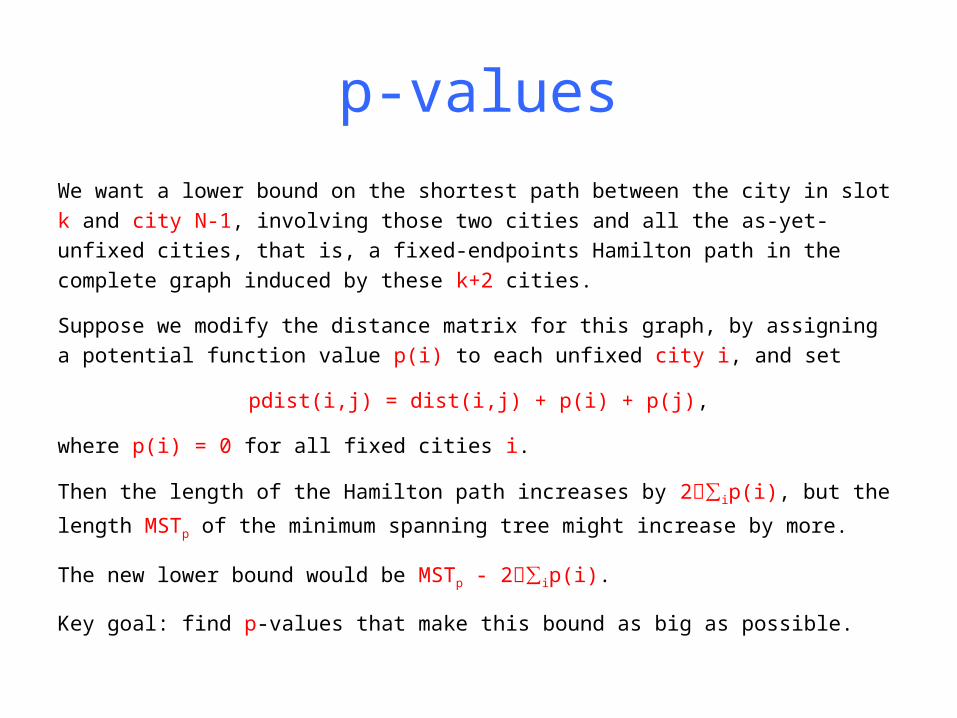
We want a lower bound on the shortest path between the city in slot k and city N-1, involving those two cities and all the as-yet-unfixed cities, that is, a fixed-endpoints Hamilton path in the complete graph induced by these k+2 cities.

Suppose we modify the distance matrix for this graph, by assigning a potential function value p(i) to each unfixed city i, and set

pdist(i,j) = dist(i,j) + p(i) + p(j),

where p(i) = 0 for all fixed cities i.

Then the length of the Hamilton path increases by 2∑ip(i), but the

length MSTp of the minimum spanning tree might increase by more.

The new lower bound would be MSTp - 2∑ip(i).

Key goal: find p-values that make this bound as big as possible.

Setting the p-values (I)

First, another observation. We can get a possibly better lower bound by

computing a value MSTp’ that might be larger than MSTp, but such that MSTp’ -

2∑ip(i) will still be a lower bound on the Hamilton path length:

• Let e1 and e2 be the two fixed endpoints for the Hamilton path (the city in

slot k and city N-1).

• Compute an MST for the unfixed vertices. Then add an edge from each ei to

the unfixed city whose p-distance to ei is minimum.

• This guarantees that the two ei both get degree 1 in the resulting tree,

something not required for an overall MST (but necessary for our Hamilton path).

Note that in the optimal Hamilton path, the edges involving the ei have to be at

least as long as the ones we chose above, and the p-length of the path of

unfixed cities linking the path neighbors of e1 and e2 (involving all the unfixed

cities) has to be at least as long as the MST for the unfixed cities.

e1 e2

d = 4

Length of overall MST = 13

Length of restricted MST = 7 + 6√2 = 15.48..

Length of min Hamilton path = 7 + 5√2 + √5 = 16.30..

Setting the p-values (II)An iterative process, starting with p(i) = 0 for all i, α = 1, and bestMST = 0.

While not yet done, do the following

1. Compute restricted MST for current p-values.

2. If MSTp’ > bestMST, do the following

1. For each unfixed city i, let deg(i) be the number of edges adjacent to city i in the current restricted MST.

2. For each unfixed city i, set p(i) = p(i) + α(deg(i) – 2).

3. Update α.

3. If α ≤ 1, quit.

4. Revert to previous p-values and update α.

Key Observations:

The value of p(i) does not change if city i already has the desired degree of 2.

It increases if deg(i) > 2, thus discouraging edges that connect to city i.

It decreases if deg(i) = 1, thus encouraging edges to connect to city i.

A Side Benefit

Theorem: Under this scheme, we will always have ∑ip(i) = 0.

(Note that this means that MSTp’ is itself our desired lower bound, with no need for adjustment.)

Proof: We start with all values equal to zero, so the claim initially holds. If there are k unfixed cities, then we have k+2 cities total, and the spanning tree has k+1 edges, for a total degree of 2k+2. This is 2k if we ignore the degrees of e1 and e2. For each unfixed city i, the change in its p-value is α(deg(i)-2), so the total change is α(∑ideq(i) – 2k) = α(2k – 2k) = 0.

Setting the p-values (III)Our heuristic scheme for updating α is the following 2-phase process.

Phase 1 (Initializing α)

1. If MSTp’ > bestMST, set α = 2α.

2. Otherwise, assuming α > 1, set α = α/2 and switch to Phase 2.

Phase 2 (Main work)

3. If MSTp’ > bestMST, leave α unchanged.

4. Otherwise, assuming α > 1, set α = α/2.

(This was the scheme used in the code supporting the paper [Johnson, McGeoch, & Rothberg, “Asymptotic Experimental Analysis for the Held-Karp Traveling Salesman Bound, Proc. 7th Ann. ACM-SIAM Symp. on Discrete Algorithms, 1996, pp. 341-350].

An AsideThis scheme was originally developed for finding lower bounds on the optimal tour, not a min cost fixed-ended Hamilton path.

To see the relationship, simply consider the case where e1 = e2, and we add the edges

from the merged city to the unfixed cities that have the first and second smallest pdist values.

Then we get a lower bound on the minimum length Hamilton cycle for the union of the

set C of unfixed cities and {e1}.

This scheme can be used basically unchanged to compute a TSP lower bound on an

arbitrary set C of cities by simply choosing some city to play the role of e1 and iterating

as previously.

It is a theorem of Held, Karp, et al. that there exists a scheme for adjusting α such that the process will converge to the solution to the LP relaxation of the TSP, no matter what

choice we make for e1.

[This is why the LP relaxation of the TSP is called the “Held-Karp bound”.]

Unfortunately, as with the results saying that simulated annealing is guaranteed to find an optimal solution, the scheme for realizing convergence to the HK bound may take exponential time…

One more thing..We can still hash solutions to avoid redundant computations, but now it is a bit more complicated.

The bound doesn’t just depend on the overall set of cities involved, but also on the identities of e1 and e2. One of the two (city N-1) is always the same, so that is not an issue, but the other (the city in slot k) can differ, and so the hash element needs to be augmented to contain not only the bitmap for the set of cities, but also the identity of the latter city.

And because of this added restriction, hashing is not nearly as effective. The median percentage of hash misses was around 40% on our testbed, versus something under 1% when we just used MST lower bounds.

Fortunately, the new lower bounds are much more effective. (On average, an increase of about 12% above the MST bound.)

At a cost of 70 extra lines of code (from 293 to 363).

Results

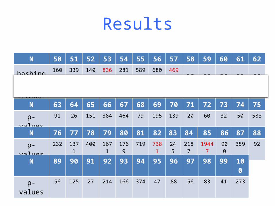
N 50 51 52 53 54 55 56 57 58 59 60 61 62hashing 1602 3397 1402 8360 2815 589 680 4699 -- -- -- -- --p-values 26 19 18 26 4.4 4.0 4.2 22 47 106 82 13 69

N 63 64 65 66 67 68 69 70 71 72 73 74 75p-values 91 26 151 384 464 79 195 139 20 60 32 50 583

N 76 77 78 79 80 81 82 83 84 85 86 87 88p-values 232 1371 400 1671 1769 719 7381 245 2187 19447 900 359 92

N 89 90 91 92 93 94 95 96 97 98 99 100p-values 56 125 27 214 166 374 47 88 56 83 41 273

Next Speedup

Maybe we were too conservative in increasing the upper bound target by 5% each time. What about 1%?(No extra lines of code!).

N 76 77 78 79 80 81 82 83 84 85 86 87 88p-values 232 1371 400 1671 1769 719 7381 245 2187 19447 900 359 92

+1% 651 7460 347 1886 1720 343 286 78 906 690 148 127 37

N 89 90 91 92 93 94 95 96 97 98 99 100 101p-values 56 125 27 214 166 374 47 88 56 83 41 273 368

+1% 17 58 30 53 46 44 18 81 73 89 45 65 99

Last Speedup (for now)

Why fool around with approximate upper bounds?

In practice, for instances this small, the best of 100 runs of Lin-Kernighan is typically optimal.

Let’s use that.

(In a shell script that runs the Johnson-McGeoch implementation of LK, finds the best of 100, and inputs that value into our exhaustive search to be used as the start value for bestlen.)

Adds less than 0.01 seconds to our running time, even for N = 150.

However, implicitly increases total lines of code by a substantial factor.

But it does let us know the limiting value of better upper bounds.

Results

N 76 77 78 79 80 81 82 83 84 85 86 87 88p-values 232 1371 400 1671 1769 719 7381 245 2187 19447 900 359 92

+1% 651 7460 347 1886 1720 343 286 78 906 690 148 127 37

LK 138 1181 196 658 625 131 160 81 355 322 131 36 24

N 89 90 91 92 93 94 95 96 97 98 99 100 101p-values 56 125 27 214 166 374 47 88 56 83 41 273 368

+1% 17 58 30 53 46 44 18 81 73 89 45 65 99

LK 20 69 30 38 27 21 22 31 34 58 39 60 103

More Results

N 102 103 104 105 106 107 108 109 110 111 112 113 114LK 170 164 199 180 222 328 313 233 1182 831 1359 2295 1798

N 115 116 117 118 119 120 121 122 123 124 125 126 127LK 1407 2359 633 886 368 2115 505 960 427 1062 1291 1512 2487

N 128 129 130 131 132 133 134 135 136 137 138 139 140LK 2574 3393 2299 2576 893 722 1979 1552 1421 5392 4658 5482 3949

N 141 142 143 144 145

146 147 148 149 150

LK 3344 7998 4498 1897 579 500 437 2185 11446 11540

More Instances

N 76 77 78 79 80 81 82 83 84 85 86 87 88LK 138 1181 196 658 625 131 160 81 355 322 131 36 24

LK-A 664 414 953 787 3945 3297 493 682 1636 1567 773 5237 444

LK-B 7 11 6 7 20 8 8 9 7 13 18 13 10

N 89 90 91 92 93 94 95 96 97 98 99 100LK 20 69 30 38 27 21 22 31 34 58 39 60

LK-A 5919 108 56 247 228 150 601 177 257 193 123 291

LK-B 25 29 12 15 27 85 282 241 498 124 177 148

Random Distance Matrices

N 27 28 29 30 31 32 33 34 35 36 37 38 39

Rand Euc 0.19 0.08 0.05 0.23 0.21 0.16 0.11 0.15

0.24 0.32 0.31

0.59 0.36

Rand Mat 0.59 0.87 5.2 5.0 6.7 2.4 67 178 11 100 59 21 6

N 40 41 42 43 44 45 46 47 48 49 50 51 52Rand Euc 0.5 0.5 0.8 1.5 2.4 1.5 1.0 2.0 3.9 2.1 2.2 2.6 3.5

Rand Mat 35 10 39 11 22 661 1353 613 4100 7343 7742 23175 14424

Note: LK (100) returned the optimal solution value in all cases.

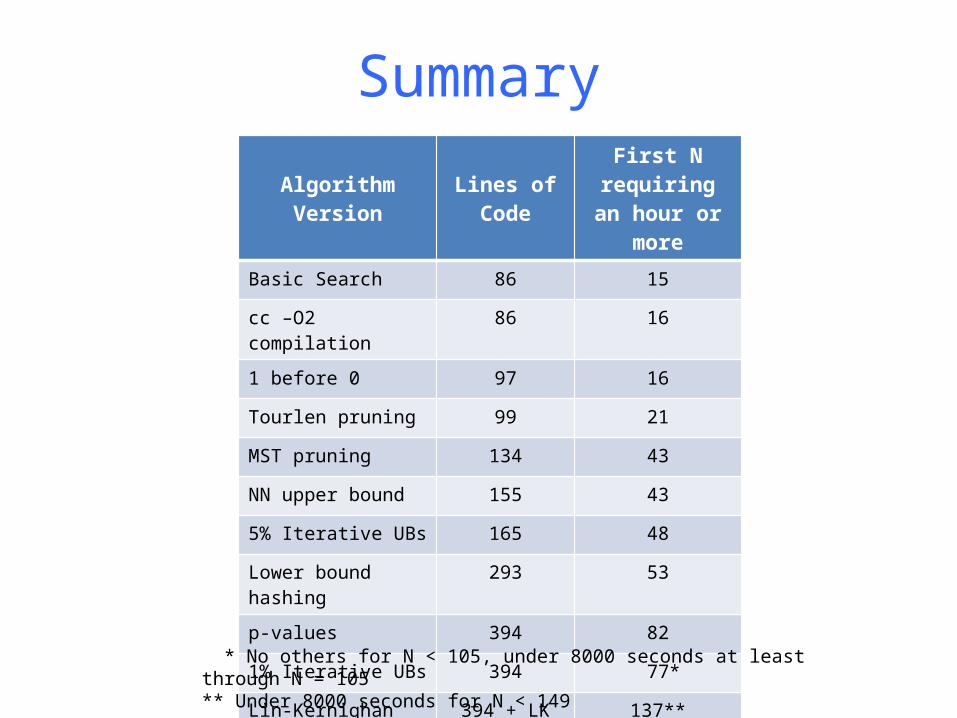
SummaryAlgorithm Version Lines of Code First N requiring

an hour or moreBasic Search 86 15

cc –O2 compilation 86 16

1 before 0 97 16

Tourlen pruning 99 21

MST pruning 134 43

NN upper bound 155 43

5% Iterative UBs 165 48

Lower bound hashing 293 53

p-values 394 82

1% Iterative UBs 394 77*

Lin-Kernighan UBs 394 + LK 137**

* No others for N < 105, under 8000 seconds at least through N = 105** Under 8000 seconds for N < 149

ConclusionsRelatively simple pruned exhaustive search over permutations can solve much bigger instances than one might naively expect.

For the hardest instance type we considered (random distance matrices) we could still find optimal solutions in minutes when N ≤ 45, and for geometric instances, we could often get beyond N = 100.

The Applegate-Cook-Dash implementation of the final version of the algorithm seems to do a bit better, perhaps due to its more sophisticated p-value scheme. This is true even though their LK implementation is less sophisticated, which enables them to include it directly in their program while keep the overall code length under 1000 lines.In particular, their code solved all the record-breaking instances that were solved before 1980 (all by LP-based methods). The 120-city Grötschel instance took their code 412 seconds.

http://www.math.uwaterloo.ca/tsp/history/milestone.html

More ObservationsConstant factor (or even linear factor) running time improvements have only a minor effect on the sizes of instances solvable (although such improvements may add up). The major impact is pruning.

Even a few percent improvement in the upper or lower bounds used in pruning can have a major impact.

The more sophisticated the algorithm, the lest predictable its results.

Adding a single city to an instance can cause an algorithm’s running time to balloon by a factor of almost 10, or shrink by a factor of almost 30.

Unfortunately, the permutation-based approach does seem to be running out of gas, and something different is needed.

N 81 82 83 84 85 86p-values 719 7381 245 2187 19447 900

Another Approach

• Branch-and-bound over sets of tour edges, not permutations.

• (This week’s “pruned exhaustive search” approach can be viewed branch-and-bound over partial permutations.)

• Lower bounds obtained by solving LP’s with a variety added inequalities (“cuts”).

• To be continued next week.

The Traveling Salesman Problem in Theory & Practice Lecture 9: Optimization 101, or “How I spent...

Documents

Transcript of The Traveling Salesman Problem in Theory & Practice Lecture 9: Optimization 101, or “How I spent...