The Transportation Revolution Revisited:

Towards a New Mapping of America's Transportation Network in

the 19th Century

Jeremy Atack

(Vanderbilt University and NBER)

Fred Bateman

(University of Georgia)

Robert A. Margo

(Boston University and NBER)

Original draft: 11/14/2007

This draft: 11/29/2007

Abstract

This preliminary paper develops a strategy for mapping the 19th century expansion of the transportation network in the United States during the nineteenth century using GIS. It focuses in particular on railroads and takes a critical look at work assessing their importance to American economic growth and development during this crucial period in our history.

The Transportation Revolution Revisited:

Towards a New Mapping of America's Transportation Network in

the 19th Century

Jeremy Atack, Fred Bateman and Robert A. Margo

Almost 200 years have now passed since Secretary of the Treasury, Albert Gallatin,

delivered his now famous report on “Roads and Canals” to Congress. According to

Gallatin, "good roads and canals will shorten distances, facilitate commercial and

personal intercourse, and unite, by still more intimate community of interests, the most

remote quarters of the United States”(Senate and Treasury 1808). The net result, he

claimed, would be an increase in national wealth and so he urged the “early and efficient

aid of the Federal (emphasis in the original) government” to mediate market failures and

externalities associated with the supply of these transportation services. Indeed, the

central importance of transportation to virtually all economic activity was “so universally

admitted, as hardly to require any additional proofs”(Senate and Treasury 1808). A

similar sentiment was re-echoed more than 50 years ago, when George Rogers Taylor

prefaced his study of the early nineteenth century improvements in transportation with

the assertion that “transportation developments were so revolutionary and so fundamental

to the growth of the country that, in my judgment, they seemed to require the central

position they have been given” (George Rogers Taylor, 1951).

Increasingly, the focus of this attention became the railroad. Indeed, a generation of

authors of American economic history texts extolled the contribution of the railroad to

American economic growth. Herman E. Krooss, for example, called the railroad “the

principal single determinant of the levels of investment, national income, and

employment in the nineteenth century” (Herman Edward Krooss, 1956); George Soule

and Vincent Carroso wrote that it “transformed the country, made possible the opening of

the continent beyond the Mississippi River, invigorated agriculture, trade and industry…a

modem industrial nation. . . would have been inconceivable without steam railroads “

(George Henry Soule and Vincent P. Carosso, 1957) and August Bolino, while calling

Max Weber’s claim that the railroad was “the greatest innovation known to mankind” an

exaggeration, nevertheless described it as “essential to the development of capitalism in

America” (August C. Bolino, 1961). Even Robert Fogel’s 1964 study of Railroads and

American Economic Development which was directed at disproving this “axiom of

indispensability” with respect to the railroad, did not dismiss the importance of

transportation per se . Even today, transport improvements continue to have a profound

effect upon economic growth and economic development, both within and across nations.

This study is motivated by several inter-related concerns and observations

concerning the role of transportation improvements in nineteenth century America during

what George Rogers Taylor famously labeled “The Transportation Revolution.” First

and foremost, transportation played a central role in shaping the nature and location of

economic activity. Second, we have an imperfect appreciation of the interaction between

different transportation modes and their respective roles in economic growth and

development. Third, there are inconsistencies in previously available data showing how

transportation diffused which creates doubts about results based upon those data. Fourth,

the recent development of geographic information systems holds promise that might

resolve these issues.

The proximate cause of this project was a perceived inconsistency between several

different sources describing the transportation network at particular benchmark dates

published in a wide variety of locations. These include contemporary maps, U.S.

government publications such as the Federal censuses, and historical atlases as well as

retrospective analyses of the role played by transportation. Among the more important of

these works are the studies by Carter Goodrich et al. (Goodrich 1961), Albert Fishlow

(Fishlow 1965), Robert W. Fogel (Fogel 1964), and Irene D. Neu and George Rogers

Taylor (Taylor and Neu 1956). More recently, a growing number of scholars are using

linked spatial data on the transportation network to examine more micro economics

estimates of the quantitative contribution of transportation improvements to land values

and economic activity (Craig 1998); (Haines 2007). At the present, most of our attention

is focused on just 4 benchmark dates, 1850, 1860, 1870 and 1880 since these coincide

with federal censuses for which we have micro-level as well as more aggregated data.

Because our ultimate goals are to explain econometrically the diffusion of

transportation modes as well as measure their economic effects at various geographic

levels, reliable data are critical. Consequently, our first step has been to take a long, hard

look at the existing information regarding the transportation network at specific moment

in time. This has proved more difficult and complex than originally anticipated despite

rapidly advancing technology. It has also proved instructive.

“ACCESS” TO TRANSPORATION MEDIA

A. Water:

Our definition of “access” is very simple: was a county adjacent to (i.e. bordered by)

or crossed by the transportation medium in question.1 Our measure of access to water

transportation is a composite of four separate “water transport” variables: proximity to

navigable rivers, canals, the Great Lakes, and the ocean. Two of these—location along

the shoreline of the Great Lakes or location on the coast—are not be subject to discussion

since proximity and access is defined purely by geographic location. The number of

counties along the Great Lakes shoreline and the oceans and Gulf of Mexico does,

however, change because county boundaries changed during the period under

consideration.2 In 1850, the area bordering the Great Lakes had been divided into 53

counties. By 1880, 78 counties occupied the same space. The number of ocean-side

counties also grew between 1850 and 1880 as large counties, particularly on the West

Coast were subdivided into more manageable units.3

We took the locations of canals from the map in Carter Goodrich (Goodrich 1961)

which shows the “principal canals in operation during the antebellum period (Figure 1)”

This map, however, is not complete for our purposes, although it appears accurate as of

1860. For example, it excludes the Santee Canal which opened in 1800 connecting the 1 Subsequently, we expand this definition to include “proximity” measured in terms of orthogonal straighline distances from the transport medium. 2 As a result, parts of larger counties that once had access may have ceased to have access when these large, unsettled counties were broken up. The growth in the number of counties with access to the Great Lakes reflects this subdivision of existing counties while maintaining Great Lakes frontage. For example Michilimackinac county in northern Michigan which straddled both the upper and lower peninsula was divided into 22 separate counties in 1860 and subsequently split up further. Not all, however, kept access to either Lake Michigan on Lake Huron, for example, Crawford and Midland counties in the interior of the Lower Peninsula. 3 For example, Trinity county on the California-Oregon border had been split into four counties—three of them, Humboldt, Klamath and Del Norte with ocean access—by 1860. These boundaries were modified further in 1874 when Klamath county was eliminated and its coastal parts absorbed by Humboldt while its interior was attached to Siskiyou County. See Thorndale.

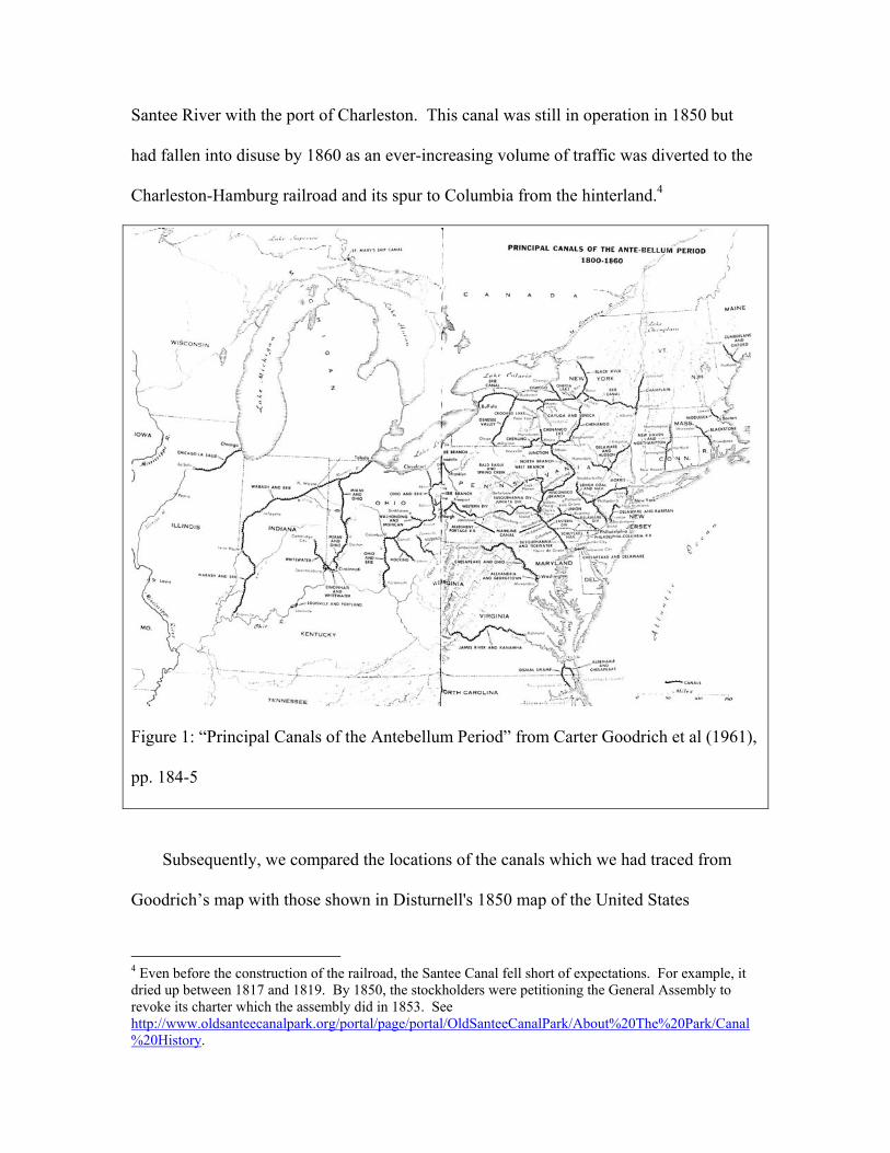
Santee River with the port of Charleston. This canal was still in operation in 1850 but

had fallen into disuse by 1860 as an ever-increasing volume of traffic was diverted to the

Charleston-Hamburg railroad and its spur to Columbia from the hinterland.4

Figure 1: “Principal Canals of the Antebellum Period” from Carter Goodrich et al (1961),

pp. 184-5

Subsequently, we compared the locations of the canals which we had traced from

Goodrich’s map with those shown in Disturnell's 1850 map of the United States

4 Even before the construction of the railroad, the Santee Canal fell short of expectations. For example, it dried up between 1817 and 1819. By 1850, the stockholders were petitioning the General Assembly to revoke its charter which the assembly did in 1853. See http://www.oldsanteecanalpark.org/portal/page/portal/OldSanteeCanalPark/About%20The%20Park/Canal%20History.

"showing all the canals, railroads, telegraph lines and principal stage routes."5 The

differences were very small, typically less than 2-3 miles and the routes often overlay one

another, criss-crossing back and forth. Consequently we have a high degree of

confidence in the location of the antebellum canals from Goodrich.

Goodrich’s map has also been supplemented with data from other sources. None of

these, however, open up new areas but rather improved existing transportation facilities. 6

Consequently, the impact of these additions to Goodrich’s canal network on our empirics

is marginal. The same is most emphatically not true of the basic canal network. Even

though canals required a steady supply of water in order to operate their locks and to

offset seepage and so were built close to where water already flowed and despite the fact

that many were constructed around obstacles on otherwise navigable rivers (such as the

Louisville and Portland Canal around the Falls of the Ohio), many of the antebellum such

as the Erie and the Wabash and Erie opened up otherwise inaccessible areas to water

navigation. As a result, their impact was separate and distinct from that of other natural

5 See g3700 ct000759 http://hdl.loc.gov/loc.gmd/g3700.ct000759 6 For example, Fogel whose map (Appendix A) is not nearly as accurately drawn as Goodrich’s but which includes a few additional canals, such as the Glen Falls feeder to the Champlain Canal which were operating by 1860, as well as later canals from the 1890 Censuses of Transportation. These later canals, however, did not open new territory to navigation prior to 1880 but rather improved existing navigation. For example, the Willamette Transportation and Lock Company project around the 40 foot falls on the Willamette River at Oregon city completed in 1873 (see, for example, http://willamettefalls.org/HisLocks) simply improved navigation on an existing navigable river as did the Des Moines Rapids canal between Keokuk and Montrose on the Mississippi River above its junction with the Des Moines River which opened for business in 1877 (New York Times, Aug. 19, 1877). The one canal that we identify as opening up new territory, the Santa Fe canal in north central Florida to the north of Gainesville did not open to traffic until 1881.

waterways.7 In addition to collecting information on the location of each canal, we also

collected information on the dates when each canal had opened for business.8

The situation was quite different with respect to navigable rivers. Here, we had to

exercise considerable judgment. Fogel took his catalog of navigable rivers and streams

from the 1890 Census of Transportation but indicated that "[I]n a goodly number of

cases, the navigable routes shown … were extended, shortened, or deleted on the basis of

information contained or references cited in U.S. Congress, House, Index to the Reports

of the Chief of Engineers, U.S. Army, 1866-1912.” Unfortunately, he did not detail what

changes he made and why in his published work. Overlaying Fogel’s map (pp. 252-3) on

the 1890 Census of Transportation map provides some clues and suggests that additions

rather than deletions were made. For example, Fogel’s map includes among the

navigable rivers the Coosa, the Conecuh and the Escambia in Alabama,9 the Edisto in

South Carolina, the Black and the Northeast rivers in North Carolina and the Dan and

Staunton in Virginia (Figure 2).10 Moreover, the 1890 Census of Transportation shows

the results of many river improvements after 1880. We have excluded these from our 7 In their analysis of the impact transportation on land values, Craig, Palmquist, and Weiss uses single composite variable "River/Canal." As we will see the effect of this is to inflate the impact of the river and to diminish the impact of the canal. 8 These dates are taken from a wide variety of different sources including Henry Varnum Poor’s History of the Railroads and Canals of the United States as well as various canal histories, county histories, and so on, many of which are available online and for which a reference or link is provided in the SHP files database. 9 Alabama adopted a large number of laws declaring various rivers and streams to be public highways and assessing penalties for blocking the same. See http://www.legislature.state.al.us/misc/History/acts_and_journals/Acts_1824/Acts_101-113.html December 14, 1824. The one steamboat known to have sailed up the Conecuh, the “Shaw,” reaching Brooklyn in 1845 was sunk on its return voyage ending all efforts at steam navigation on the river. http://ftp.rootsweb.com/pub/usgenweb/al/conecuh/history/other/gms36historyo.txt . The Coosa was largely impassable to river traffic between Wetumpka (a little above the junction with the Alabama River and Greensport in St. Clair county (now submerged). See map of river at http://alabamamaps.ua.edu/historicalmaps/alrivers/index.html “Coosa River from Greensport to Wetumpka” 10 The Dan and the Staunton both had batteau navigation early in the century but were not navigable by steam until the 1880s (and then only briefly). See “Steamboats on the Staunton,” The Tiller, Vol. 17, Issue 3 - Fall 1996 by The Virginia Canals and Navigating Society republished at http://www.oldhalifax.com/county/StauntonSteamboat.htm and http://www.danriver.org/ .

data set. We have interpreted “navigation” to mean regular (or rather something other

than an a one time or very rare occurrence) traffic both up and downsteam. Thus, for

example, while Fogel shows the head of navigation on the Arkansas River as Wichita,

Kansas, we can find no record of steam navigation beyond Fort Smith on the Arkansas.

Similarly, Fogel has Gainesville, Texas as the head of navigation on the Red River but

few, if any boats, ventured above Fulton, Arkansas prior to the 1880s and during the

antebellum period, Shreveport was the practical head.11 Moreover, we can find no record

of steam navigation on the Cumberland River in Tennessee above Carthage while Hunter

dismisses navigation on the Licking and Big Sandy Rivers in Kentucky noting “small

steamboats occasionally ran for short distances.”12

At the same time, the 1890 Census of Transportation map excludes a least one river

where there is known to have been active navigation during the period: the Wisconsin

River (see Figure 2). As a result, this river is not included in Fogel's analysis. In

nineteenth century, however, steamboats navigated the Wisconsin River from its junction

11 Hunter, p 51 12 The kind of evidence one finds regarding steamboat operations during the 19th century is as follows. On the Pearl River in Mississippi, for example, we know that in 1880 Congress authorized the dredging of a 5 foot navigation channel from Jackson to the Gulf. Prior to that date there is evidence of intermittent steam boats operations on the river. For example in May 1838 steamboats “Alice Maria” brought lumber up the river to Jackson to build the first state capital and in the early 1840s Marcus Hilzheim announced that he would run a small schema from Carthage to New Orleans. In 1848 steamboat “Caroline” operating as "Pearl River steam packet" so the river however there is no other boat recorded on the a proposal until 10 years later when the steamboat “Ranger” caught fire and was lost. Keel boats were used on the river before and after the Civil War and small steamboats made a regular runs to cottage in the 1870s. (http://www.rootsweb.com/~msleake/pearl_river.html) According to Transportation in the American Frontier (Sherri M.L. Smith), the first steamboat to travel the Apalachicola-Chattahoochee-Flint River System appeared in 1828. Steamboats regularly traveled the Chattahoochee as far as Columbus, the head of navigation on that river, and served more than a 100-mile stretch of the lower Flint. By 1860 more than 26 steamboat landings dotted the Flint between its junction with Chattahoochee and Bainbridge ... smaller boats and barges traveled the water from Bainbridge to Albany...Steamboats continued to thrive in the 1850s despite the competition of railroads, and remained in operation until about 1928. On the other hand, according to the Corps of Engineers, the Flint River is only navigable at low water from its mouth up as far as Bainbridge. Beginning in 1873 the Corps of Engineers began an effort to improve navigation on the river and secured a 3 foot deep channel at least 50 feet wide as high as Albany by 1890. See the Annual Reports on the Secretary of War 1891, page 198.

with the Mississippi River at as least as far as Portage in Columbia county (and close to

the head of navigation of the Fox River) and maybe went as high as Nekoosa in Wood

county.13

Figure 2: Fogel’s “Extended System of Navigation” (Fogel 1964, pp. 252-3) Overlayed

upon the 1890 Census of Transportation map of Navigable Rivers

Our summary of the number of counties served by navigable waterways appears as

Table 1 and is shown in Figure 3. In addition to measuring whether or not a particular

county had access to one or more of the water transport media at each of the benchmark

dates, we have also computed a single dummy variable, "navigable waterway" which

takes a value of one whenever any county is served by any kind of navigable waterway.

13 http://www.hmdb.org/marker.asp?marker=1193

Table 1: Number of counties with “access” to navigable water

1850 1860 1870 1880

Great Lakes 53 71 74 78

Gulf and oceans 174 198 202 205

Navigable Rivers 566 667 684 731

Canals 197 225 226 227

Any Water 833 989 1,014 1,067

These counts prove to be quite different from those made by other scholars. At this

stage we have not tried to reproduce the sample of 1,529 counties in 1850 used by Craig,

Palmquist and Weiss (CPW) exactly but, if we exclude those counties lying beyond about

the 98th line of longitude, we end up with a sample of 1,548 counties. In their sample,

CPW determined that 540 counties (=1,529 x .353 -- see Table 2) had access either to a

river or a canal. In our slightly larger sample, we count 752 such counties. They identify

119 counties along the Atlantic and Gulf coasts (= 1,529 x 0.078), we show 152.14

The 1850 ICPSR file assembled by Haines based upon the CPW data, lists 736 of the

1,616 counties as being located along a navigable waterway. Using our GIS-encoded

data, we count 833. Similarly, in 1860, the Haines ICPSR file has 871 of the 2,076

counties as being located along a navigable waterway compared with our estimate of 989.

In each year, we classify some counties as lacking navigable water access which Haines

and CPW classify as having water access and vice versa. In 1850, we agree that a

common core of 671 counties had water access. In 1860, we agree on 813 counties.

14 Since, according to the maps, the entire eastern seaboard was included in their sample, our counts should agree in this instances despite any differences in our underlying samples.

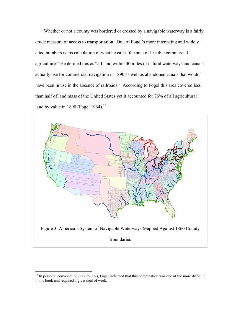
Whether or not a county was bordered or crossed by a navigable waterway is a fairly

crude measure of access to transportation. One of Fogel’s more interesting and widely

cited numbers is his calculation of what he calls “the area of feasible commercial

agriculture.” He defined this as “all land within 40 miles of natural waterways and canals

actually use for commercial navigation in 1890 as well as abandoned canals that would

have been in use in the absence of railroads." According to Fogel this area covered less

than half of land mass of the United States yet it accounted for 76% of all agricultural

land by value in 1890 (Fogel 1964).15

Figure 3: America’s System of Navigable Waterways Mapped Against 1860 County

Boundaries

15 In personal conversation (1129/2007), Fogel indicated that this computation was one of the more difficult in the book and required a great deal of work.

We have used some of the more sophisticated capabilities of ArcGIS to calculate the

equivalent figure for earlier benchmark dates.16 Excepting the Gadsden Purchase in

1853, the territorial area of the lower 48 states did not change during the period in

question. Imposing a 40 mile wide buffer similar to that used by Fogel around each

navigable waterway, we estimate that 41.9 percent of the land mass lay within that

boundary. This same area, however, contained at least 80.9 percent of the nation’s

population and 80.2 percent of the value of her farmland as of 1880, as well as more than

93 percent of the nation’s industrial production. Given the time trend in the data, Fogel’s

figure of 76% of farmland by value lying within 40 miles of a navigable waterway in

1890 is entirely plausible despite differences in our definitions in “navigable.” Moreover,

these estimates are lower-bound estimates in so far as they implicitly assume that farm

value, etc. was uniformly distributed across the county whereas, in reality, it was

concentrated around population centers which in turn was clustered around transportation

media, especially breaks in transportation and transportation mode. At earlier dates, the

fractions were generally somewhat higher as the relentless expansion of the railroad into

otherwise inaccessible territory drew population and economic activity into those areas.

Collectively, these data suggest that one consequence of the advent of the railroad and the

16 These estimates are made by dissolving the individual features into a single composite feature, establishing the appropriate buffer around that feature, and then computing the intersection between that feature and the individual county boundaries. We then calculated the aggregate sum of the areas within the buffers for each county as a fraction of the area of the county and weight appropriately by the relevant variable. The procedure was as follows: To create the shape files in ArcGIS, we first dissolved the features using DataManagement/Generalization to create a single composite feature. We then used AnalysisTools/Proximity to the create the buffer and, finally, AnalysisTools/Intersect to create the final file which contains the portions of the buffer around each feature that fall within a particular county. The “Calculate Geometry” option within the Attribute Table can then be used to calculate the area of the boundary. Finally, Stat/Transfer was used to create STATA files from the DBF files for the county SHP files and these were joined using FIPS codes to the feature boundary file and also to the ICPSR files assembled by Michael Haines. We calculated the ratio of the feature boundary to the entire county and tabulated on state using the appropriate variable as weights and summarizing using this ratio in STATA.

spread of the rail network was to disperse economic activity across the United States in

the same manner by which transportation improvements generate a flattening of the rental

price gradient.

Table 2: The Fraction of U.S. Land, Population, Farmland, Farm Value, etc. Located

(Produced or Residing) Within a Specific Distance of a Navigable Waterway 1850 1860 1870 1880WITHIN 40 “AIRLINE” MILES Variable Land 41.9Population 87.5 85.4 84.0 80.9Farmland 81.8 78.3 76.7 70.7Farm Value 90.5 87.4 85.4 80.2Manufacturing Output 95.3 94.2 94.1 93.7Real Estate 89.3 Personal Estate 86.2 "True value of real and personal estate" 90.7 WITHIN 15 “AIRLINE” MILES 1850 1860 1870 1880Variable Land 20.8Population 58.2 56.9 56.1 54.2Farmland 46.4 43.0 41.5 37.4Farm Value 60.3 55.6 52.7 48.0Manufacturing Output 76.9 76.1 76.4 77.3Real Estate 62.5 Personal Estate 39.4 "True value of real and personal estate" 69.4 See footnote 15 for a description of the ArcGIS procedures used.

Whether or not a 40 airline-mile buffer represents a reasonable distance for wagon

haulage depends in part upon one's objective. Certainly, it exceeded the average distance

that New England’s farmers travelled to market during the antebellum period despite

having some of the best roads in the nation. Such a journey would have several days by

oxen or horse-drawn wagon. According to the farmers’ account books surveyed by

Rothenberg, the median trip to market between 1821 and 1855 was 14 miles, with an

average of between 20 and 25 miles(Rothenberg 1981). This figure is also consistent

with estimates at the dawn of the motor age that 11 miles a day was the practical limit for

horse haulage with a two ton truck; 9 miles with a five ton truck.17 Similarly, 15 miles

was quoted as a good day’s travel on the Oregon Trail. For passenger travel, distances

were higher. For example, according to an 1849 travel guide, it took 2 days by stage to

travel the 167 miles from Chicago to Galena (Williams and D. Appleton and Company.

1849). Such a trip would also have required several changes of horse teams.

Reducing the size of the buffer reduces the fraction of the population, farm land,

farm value, etc. lying within the “feasible region.” Trimming the buffer to 15 miles

reduces the share of the land mass within this area to 20.8%. However, almost 50% of

farmland by value lay within this area which also contributed about three-quarters of the

nation’s manufacturing output. Clearly, one important conclusion from these data is that

proximity to water transportation was strongly and positively associated with many

different forms of economic activity and wealth.

B. Railroads

What, then, of the new transportation media, the railroads? Since water resources

were heavily concentrated in the eastern part of the country and this was, initially, the

only settled part of the country it would seem inevitable that the railroad as a latecomer to

the scene would follow rather than lead—at least initially, especially when such large

fractions of economic activity and resources were located in such close proximity to

water.

17 According to the New York Times at the dawn of the motor age “the limit of profitable horse haulage per day is placed at eleven miles for a two-ton truck and nine miles for a five-ton truck” “Motor Trucks to Supplant Horse Drawn Vehicles,” New York Times, March 20, 1910, p. S4. Fifteen miles is quoted as a good days’ travel on the Oregon Trail

Locating and documenting the railroads in operation during the nineteenth century

proved much more difficult and uncertain than dealing with navigable waterways.

Indeed, writing in 1914, Paxson (Paxson 1914) remarked “It would be dangerous to say

that no accurate railroad maps exist for the period before the civil war, but it is certain

that such are in frequent use … for even the most commonplace facts … the investigator

must go to scattered, incomplete, and inaccurate sources, which, at best, are to be found

in only a few of the greatest libraries.”

To date we have relied upon digitized railroad maps, primarily those at the Library of

Congress, which we have geo-referenced to historical SHP files showing county

boundaries at benchmark census dates.18 Errors arise from multiple distinct sources.

First, the dates on many maps tend to be ambiguous. Most list their copyright date rather

than the date represented by the data contained in the map. Moreover, mapmakers were

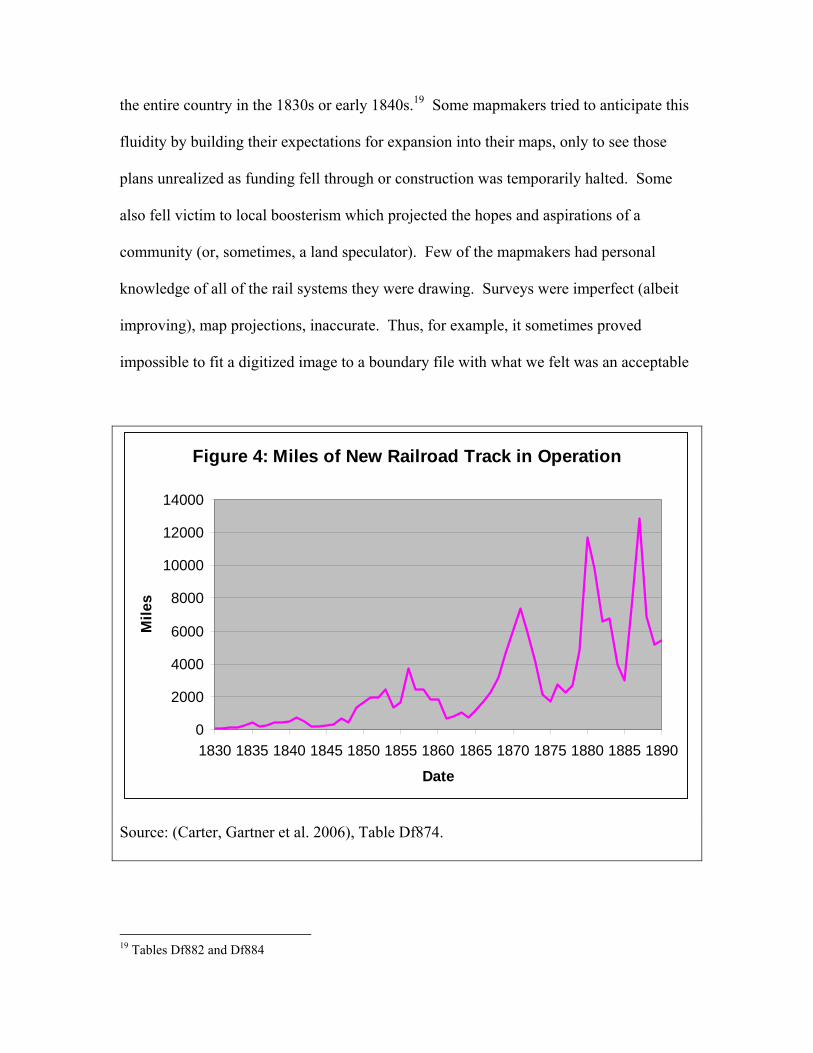
attempting to capture a flow—railroad construction—as a snapshot. For example, in each

year from 1848 through 1861 and from 1868 through 1879, more than a thousand miles

of track was built. In some years, most notably 1872, many thousands of miles were built

and there were years in the 1880s when more than 10,000 miles of new track was added

(Figure 4). Thus, even the most accurately drawn map which spent a month or two in

production might miss more new railroad mileage during these years than had existed in

18 When we began work on this project, SHP files were not yet available from the NHGIS at the University of Minnesota and so we made use of the HUSCO SHP files as modified and updated by Haines. One serious disadvantage of the HUSCO files is that they contain no projection information and so cannot easily be linked to modern GIS data. Specifically, modern GIS layers do not overlay properly on the HUSCO SHP files. The HUSCO files do however have two distinct advantages. First, they link seamlessly to the Haines’s ICPSR data sets. Second, these files are relatively small and redraw quickly. The NHGIS files on the other hand a much more detailed, much larger, and align perfectly with other GIS layers. With the assistance of a projection specialist at ERSI we have found a transformation and projection, albeit currently imperfect, which brings the HUSCO files close to but not yet coincident with the NHGIS files.

the entire country in the 1830s or early 1840s.19 Some mapmakers tried to anticipate this

fluidity by building their expectations for expansion into their maps, only to see those

plans unrealized as funding fell through or construction was temporarily halted. Some

also fell victim to local boosterism which projected the hopes and aspirations of a

community (or, sometimes, a land speculator). Few of the mapmakers had personal

knowledge of all of the rail systems they were drawing. Surveys were imperfect (albeit

improving), map projections, inaccurate. Thus, for example, it sometimes proved

impossible to fit a digitized image to a boundary file with what we felt was an acceptable

Figure 4: Miles of New Railroad Track in Operation

0

2000

4000

6000

8000

10000

12000

14000

1830 1835 1840 1845 1850 1855 1860 1865 1870 1875 1880 1885 1890

Date

Mile

s

Source: (Carter, Gartner et al. 2006), Table Df874.

19 Tables Df882 and Df884

degree of precision.20 Last, and certainly not least, rail lines were not accurately and

consistently drawn on maps with the result that railroads seemed to shift location from

year to year. Some, of course, may have been realigned and re-graded. For example,

following the merger of Boston and Lowell Railroad with the Boston and Maine in 1845,

track between Wilmington and Boston was initially abandoned (only to be later reused by

the B&L for their Wildcat Branch). In 1848, the Boston and Maine abandoned another

original section of track as a new alignment was built from Wilmington north to North

Andover so as to better serve Lawrence. In 1873, a new alignment to Portland was

opened splitting from the old route at South Berwick and the old route was subsequently

abandoned.21 However, in most cases, once a railroad was built; there it stayed put

because the bulk of the investment was not just fixed but also sunk. For example,

according to the 1880 Census, over 80 percent of railroad investment went in

construction costs, of which only one or two percent represented the cost of the land

itself, the rest went in surveying, grading, removing or bridging obstacles and laying the

track. While ties, ballast and the rails might be reused and the land could be resold, the

grading, cuttings, embankments, bridges, and drainage ditches had few alternative uses—

especially in the nineteenth century.22 Indeed, railroads today still follow many of the

routes blazed by the nineteenth century railroads although Paxson cautioned “nearly

every road has straightened out and shortened its line since 1860 (Paxson 1914).23

20 Our goal was to have no more than a 5 mile difference between known reference points though sometimes we settled for more. Folded maps that had been split apart and reassembled using fabric hinges where the folds used to be proved especially challenging and had to be geo-referenced in sections rather than as a whole. 21 http://www.answers.com/topic/boston-and-maine-railroad 22 Nowadays, of course, they find recreational uses in the “rails to trails” movement 23 And, of course, thanks to GIS, these can be quite precisely located. One might thus be tempted to begin with modern railroad maps and force the nineteenth century locations to conform to these. On average, this

Probably the best nineteenth century railroad maps were those which appeared in

“pocket” travel guides.24 Appearing first in the 1840s, some were published monthly;

others, semi-annually or annually, often under slightly changed names. These include

Disturnell's Railroad, Steamboat and Telegraph Guide (1846) (Disturnell 1847),

Doggett's Railroad Guide and Gazetteer (1847) (Doggett 1848)and Appletons' Railway

and Steam Navigation Guide (1848) (D. Appleton and Company.), Dinsmore's American

Railway Guide (1850) (Cobb and Fisher 1851), Lloyd's American Guide (1857) (Lloyd

1857), Travelers' Official Railway Guide (1868) (Vernon and National General Ticket

Agents' Association. 1871) and The Rand-McNally Official Railway Guide and

Handbook (1871) (Rand McNally and Company., National General Ticket Agents'

Association. et al. 1879). Each went through many editions. Unfortunately, as

ephemera, relatively few have survived and we have yet to assemble enough of them to

construct an accurate time series.25 All are fragile, especially the multi-page fold-out

maps. A few of these guides, however, have been digitized.26 Competition and frequent

publication should have ensured that only the more useful of these guides survived.

Dinsmore’s guide, for example, was singled out for praise by one of the leading

commercial/business publishers of the time: Hunt’s Merchants’ Magazine.

is probably a good strategy even though it would misrepresent earlier track locations that were changed through realignments such as that described above. 24 Indeed, such sources were used by Taylor and Neu Taylor, G. R. and I. D. Neu (1956). The American railroad network, 1861-1890. Cambridge,, Harvard University Press. in drawing up their maps of the US rail network as of April 1861 25 Even in 1914, Paxson while noting that the “value to the purchaser depended entirely upon its fidelity in describbing actual running arrangements … unfortunately the number of copies that escaped destruction is small” Paxson, F. L. (1914). "The Railroads of the "Old Northwest" before the Civil Wat." Transactions of the Wisconsin Academy of Sciences, Arts, and Letters 17(Part 1): 247-274.. 26 See, for example, the June 1870 copy of the Travelers’ Official Railway Guide at http://cprr.org/Museum/Books/I_ACCEPT_the_User_Agreement/Travellers_Guide_6-1870.pdf from the Central Pacific Railroad Museum. There are also at least two different editions of Appleton’s Guide on Google Books such as http://books.google.com/books?vid=UOM39015016751375 as well as a number of other guides. See http://www.lib.utexas.edu/maps/map_sites/hist_guide_sites.html

We are indebted to the publishers for a copy of the last number of their NEW GUIDE ;

and must say that for conciseness, mingled with complete information, neatness of

execution, and convenience of reference, it fully equals our expectations of what a

Railroad Guide should bе. Besides the usual tables of distances, times, and fares, the

traveler is provided with a handsome and complete railroad map of the whole country,

and small maps of the great centers and trunk lines, with tables of reference to the details

of the lines represented on them, and very perfect tables of steamboat lines on the

principal rivers and waters ; and appended to the whole is an excellent Railroad

Gazetteer. Dinsmore, as he has always done, keeps up with the times ; and it is a great

inducement for him to do so, that he may furnish correct information for those whose

lack of originality leads them to copy from him. We can unhesitatingly recommend

Dinsmore's American Railroad and Steam Navigation Guide. (Hunt’s Merchants’

Magazine, 36, January-June 1857. p253)

As the editor of Hunts’ Magazine noted, many guides contained multiple large scale

maps. These often covered quite small areas, providing details such as bridges and

tunnels that are not easily seen on other, larger maps such as those in the Library of

Congress’ “American Memory” railroad collection. Moreover, these maps emphasize the

disconnected nature of America’s railroads and other complexities of nineteenth century

travel.27 For example, travelers switching trains between systems generally had to switch

stations prior to the “Union station” movement which gathered steam after the Civil War

(Bianculli 2001).

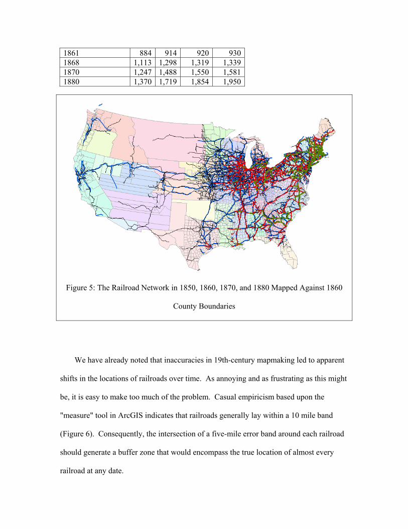
The data in Table 3 (some of which are mapped in Figure 5) represents a crude

measure of the spread of the railroad network by showing the number of counties (as of 27 For example, the prevalence of local time. According to a chart in Appleton’s Guide, for example, when it was noon in New York, it was 11:10 in Indianapolis, 11:19 in Cincinnati, 11:24 in Columbus, 11:30 in Cleveland, 11:36 in Pittsburgh, 11:56 in Philadelphia, and 12:12 in Boston—that is to say, local time was defined relative to the sun at midday .

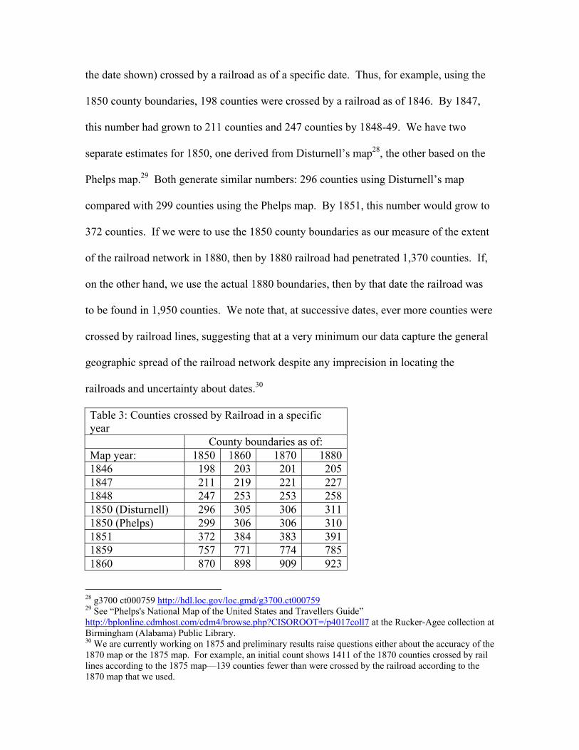
the date shown) crossed by a railroad as of a specific date. Thus, for example, using the

1850 county boundaries, 198 counties were crossed by a railroad as of 1846. By 1847,

this number had grown to 211 counties and 247 counties by 1848-49. We have two

separate estimates for 1850, one derived from Disturnell’s map28, the other based on the

Phelps map.29 Both generate similar numbers: 296 counties using Disturnell’s map

compared with 299 counties using the Phelps map. By 1851, this number would grow to

372 counties. If we were to use the 1850 county boundaries as our measure of the extent

of the railroad network in 1880, then by 1880 railroad had penetrated 1,370 counties. If,

on the other hand, we use the actual 1880 boundaries, then by that date the railroad was

to be found in 1,950 counties. We note that, at successive dates, ever more counties were

crossed by railroad lines, suggesting that at a very minimum our data capture the general

geographic spread of the railroad network despite any imprecision in locating the

railroads and uncertainty about dates.30

Table 3: Counties crossed by Railroad in a specific year County boundaries as of: Map year: 1850 1860 1870 18801846 198 203 201 2051847 211 219 221 2271848 247 253 253 2581850 (Disturnell) 296 305 306 3111850 (Phelps) 299 306 306 3101851 372 384 383 3911859 757 771 774 7851860 870 898 909 923

28 g3700 ct000759 http://hdl.loc.gov/loc.gmd/g3700.ct000759 29 See “Phelps's National Map of the United States and Travellers Guide” http://bplonline.cdmhost.com/cdm4/browse.php?CISOROOT=/p4017coll7 at the Rucker-Agee collection at Birmingham (Alabama) Public Library. 30 We are currently working on 1875 and preliminary results raise questions either about the accuracy of the 1870 map or the 1875 map. For example, an initial count shows 1411 of the 1870 counties crossed by rail lines according to the 1875 map—139 counties fewer than were crossed by the railroad according to the 1870 map that we used.

1861 884 914 920 9301868 1,113 1,298 1,319 1,3391870 1,247 1,488 1,550 1,5811880 1,370 1,719 1,854 1,950

Figure 5: The Railroad Network in 1850, 1860, 1870, and 1880 Mapped Against 1860

County Boundaries

We have already noted that inaccuracies in 19th-century mapmaking led to apparent

shifts in the locations of railroads over time. As annoying and as frustrating as this might

be, it is easy to make too much of the problem. Casual empiricism based upon the

"measure" tool in ArcGIS indicates that railroads generally lay within a 10 mile band

(Figure 6). Consequently, the intersection of a five-mile error band around each railroad

should generate a buffer zone that would encompass the true location of almost every

railroad at any date.

Figure 6: Illustration of the Shifting Location of Rail Lines (Central Ohio). Depth of

“Band” Containing Railroads Between Sets of Points Is About 8 Miles

The procedure outlined above stands in sharp contrast to that used by CPW in

deriving their original series of access to water and rail transportation. They adopted the

time-honored method of eyeballing the data and making judgment calls regarding the

precise path followed by a transportation route, sometimes in the absence of county

boundaries on most maps. Furthermore, they endeavored to integrate multiple maps

covering different years and different parts of the country into a single measure.31 Using

31 The procedures used by CPW were as follow: “The way in which the counties were coded was simple: I reserved space in our library's map room one summer ('96, I think). I then collected histories containing maps of transporation improvements in general and the railroad industry in particular. (These include the histories cited in the JREFE article in the issue you edited.) I also had the librarians dig out old maps that had county lines on them. (I don't think these maps are cited in the paper. In fact, there were many of them and the librarians just laid them out for

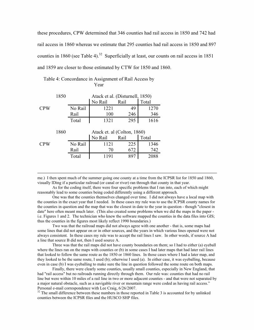
these procedures, CPW determined that 346 counties had rail access in 1850 and 742 had

rail access in 1860 whereas we estimate that 295 counties had rail access in 1850 and 897

counties in 1860 (see Table 4).32 Superficially at least, our counts on rail access in 1851

and 1859 are closer to those estimated by CTW for 1850 and 1860.

Table 4: Concordance in Assignment of Rail Access by Year

1850 Atack et al. (Disturnell, 1850)

No Rail Rail Total CPW No Rail 1221 49 1270 Rail 100 246 346 Total 1321 295 1616

1860 Atack et. al (Colton, 1860) No Rail Rail Total CPW No Rail 1121 225 1346 Rail 70 672 742 Total 1191 897 2088

me.) I then spent much of the summer going one county at a time from the ICPSR list for 1850 and 1860, visually IDing if a particular railroad (or canal or river) ran through that county in that year. As for the coding itself, there were four specific problems that I ran into, each of which might reasonably lead to some counties being coded differently using a different approach. One was that the counties themselves changed over time. I did not always have a local map with the counties in the exact year that I needed. In these cases my rule was to use the ICPSR county names for the counties in question and the map that was the closest in date to the year in question - though "closest in date" here often meant much later. (This also created some problems when we did the maps in the paper - i.e. Figures 1 and 2. The technician who knew the software mapped the counties in the data files into GIS; thus the counties in the figures most likely reflect 1990 boundaries.) Two was that the railroad maps did not always agree with one another - that is, some maps had some lines that did not appear on or in other sources, and the years in which various lines opened were not always consistent. In these cases my rule was to accept the rail lines I saw. In other words, if source A had a line that source B did not, then I used source A. Three was that the rail maps did not have county boundaries on them; so I had to either (a) eyeball where the lines ran on the maps with counties or (b) in some cases I had later maps that had later rail lines that looked to follow the same route as the 1850 or 1860 lines. In those cases where I had a later map, and they looked to be the same route, I used (b); otherwise I used (a). In either case, it was eyeballing, because even in case (b) I was eyeballing to make sure the line in question followed the some route on both maps. Finally, there were clearly some counties, usually small counties, especially in New England, that had "rail access" but no railroads running directly through them. Our rule was: counties that had no rail line but were within 10 miles of a rail line in two or more adjacent counties - and that were not separated by a major natural obstacle, such as a navigable river or mountain range were coded as having rail access.” Personal e-mail correspondence with Lee Craig, 6/26/2007. 32 The small difference between these numbers in those reported in Table 3 is accounted for by unlinked counties between the ICPSR files and the HUSCO SHP files.

THE IMPACT OF TRANSPORTATION ACCESS ON LAND VALUES

Given the differences in procedures, differences in the outcomes are not surprising.

Our immediate question here is whether these differences lead to meaningful differences

in the results and conclusions.

CPW estimated a hedonic pricing model in semi-logarithmic form to examine the

determinants of the equilibrium price schedule for land. The dependent variable in their

model was the log of the value of farmland per acre and the independent variables of

particular interest were dummy variables for access to river or canal transportation

(combined into a single variable), the ocean and the Great Lakes, and access to rail

transportation. Their model included a number of other independent variables thought to

affect the value of land including the presence of or proximity to large urban areas and

population density.

Rather than try to duplicate their results, we have instead estimated a version of their

equation using only the variables contained within the Haines ICPSR file which

combines all water transportation into a single dummy variable. We have done the same

with our data on access to transportation which we have described above although we

also make estimates using separate variables for location along rivers, canals, the shores

of the Great Lakes or the ocean.

Table 5 reports two of the CPW hedonic estimates together with our estimate of the

equivalent equation using an expanded sample of counties and the collapsed version of

their variable for access to water and access to rail. Our model also excludes the crop

dummies and replaces the urban dummies with the percentage of the county’s population

living in an urban area, defined as a incorporated area with at least 2,500 population.

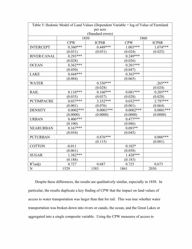
Table 5: Hedonic Model of Land Values (Dependent Variable = log of Value of Farmland per acre

(Standard errors) 1850 1860 CPW ICPSR CPW ICPSR INTERCEPT 0.360*** 0.449*** 1.003*** 1.074*** (0.031) (0.031) (0.024) (0.025) RIVER/CANAL 0.293*** 0.249*** (0.028) (0.026) OCEAN 0.362*** 0.201*** (0.050) (0.047) LAKE 0.444*** 0.363*** (0.084) (0.065) WATER 0.330*** .265*** (0.028) (0.024) RAIL 0.110*** 0.160*** 0.081*** 0.205*** (0.035) (0.037) (0.028) (0.028) PCTIMPACRE 0.037*** 3.352*** 0.032*** 2.797*** (0.001) (0.076) (0.001) (0.064) DENSITY 0.0002*** 0.0001*** 0.0002*** 0.0001*** (0.0000) (0.0000) (0.0000) (0.0000) URBAN 0.406*** 0.477*** (0.100) (0.086) NEARURBAN 0.167*** 0.093** (0.054) (0.045) PCTURBAN 0.876*** 0.006*** (0.115) (0.001) COTTON -0.011 0.102* (0.061) (0.058) SUGAR 1.382*** 1.428*** (0.188) (0.183) R2(adj) 0.727 0.687 0.725 0.673 N 1529 1583 1861 2030

Despite these differences, the results are qualitatively similar, especially in 1850. In

particular, the results duplicate a key finding of CPW that the impact on land values of

access to water transportation was larger than that for rail. This was true whether water

transportation was broken down into rivers or canals, the ocean, and the Great Lakes or

aggregated into a single composite variable. Using the CPW measures of access to

different transportation media, the results in Table 5 suggests that water access raised the

value of land by 39% in 1850 and by 30% in 1860. The rail access also raised the price

of land but by less than access to water, probably reflecting the fact that water

transportation costs only a fraction of rail transportation, a consideration was likely of

particular importance for bulky, relatively low-value-to-weight agricultural commodities.

Our results using CPW’s definition of rail access indicate that having access to a railroad

raised the price of land in the county by 17% in 1850 over that in an otherwise identical

county lacking this transportation medium. In 1860, rail access raised the price of land by

23%, a figure significantly higher than that estimated by CPW. This difference may

reflect our inclusion of more western counties where land, prior to the advent of the

railroad, had little or no value.

If we redo these same hedonic regressions using our GIS-based measures of access

to transportation, we find the impact of access to water much attenuated particularly in

1850 from the figures reported in Table 5. More importantly, our estimates extend to

1870 and 1880 and in these years, we find the impact of water and rail reversed from that

at earlier years. The results reported in Table 6. In 1850, rail access raised the price of

land by 13% compared with 31% for water access. In 1860 rail access raised the value of

land by more than 20% while water access raised the price of land by almost 27%.

Beginning in 1870, however, rail access had a much larger effect than water access. In

1870, for example, rail access raised the value of land by 56% compared with just 26%

for water access. The impact of rail transportation was smaller in 1880, "only" 32%

compared to water’s impact of 22%. Thinking about the explosion of rail construction

into the West during the late 1860s and the 1870s and the general impossibility of

expanding water navigation into these same areas, we believe that these results are

plausible.

Table 6: Hedonic Model of Land Value: GIS-based measures (Standard errors)

Variable 1850 1860 1870 1880% Urban 0.962 0.007 0.239 1.162 (0.116) (0.001) (0.047) (0.074)% Improved 3.453 2.856 3.395 2.868 (0.076) (0.064) (0.072) (0.054)Rail Access 0.123 0.187 0.444 0.281 (0.039) (0.027) (0.035) (0.030)Water Access 0.270 0.239 0.233 0.201 (0.028) (0.024) (0.031) (0.024)Population Density 0.0001 0.0001 0.0001 0.0001 (0.000) (0.000) (0.000) (0.000)Intercept 0.433 1.039 0.520 0.553 (0.032) (0.025) (0.035) (0.031)R2(adj) 0.675 0.673 0.636 0.685N 1585 2031 2230 2497Numbers in bold indicate statistical significance at better than the 99% level

The size of rail's impact on the value of land is largely unchanged when we separate

out different forms of water transportation. Our conclusion, however, with regard to the

impact of navigable waterways changes dramatically. The economic importance of rivers

was declining over the time while the economic importance of canals and Great Lakes

transportation was large and rising, exceeding the impact of rail in each year. These

results are shown in Table 7 which simply reports the percentage change in the value of

land attributable to access to a particular transportation medium in a given year, without

reporting the other variables in the equation.33 These figures warrant further analysis and

represent a potential reinterpretation of transportation history.

33 These other variables with the same as those reported in Table 6.

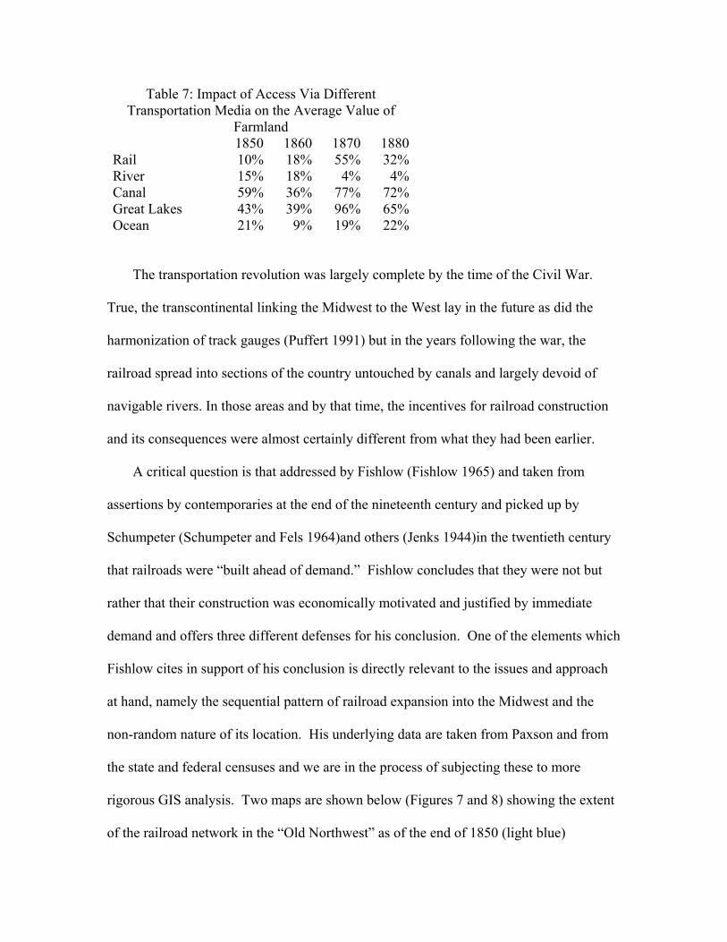
Table 7: Impact of Access Via Different Transportation Media on the Average Value of

Farmland 1850 1860 1870 1880Rail 10% 18% 55% 32%River 15% 18% 4% 4%Canal 59% 36% 77% 72%Great Lakes 43% 39% 96% 65%Ocean 21% 9% 19% 22%

The transportation revolution was largely complete by the time of the Civil War.

True, the transcontinental linking the Midwest to the West lay in the future as did the

harmonization of track gauges (Puffert 1991) but in the years following the war, the

railroad spread into sections of the country untouched by canals and largely devoid of

navigable rivers. In those areas and by that time, the incentives for railroad construction

and its consequences were almost certainly different from what they had been earlier.

A critical question is that addressed by Fishlow (Fishlow 1965) and taken from

assertions by contemporaries at the end of the nineteenth century and picked up by

Schumpeter (Schumpeter and Fels 1964)and others (Jenks 1944)in the twentieth century

that railroads were “built ahead of demand.” Fishlow concludes that they were not but

rather that their construction was economically motivated and justified by immediate

demand and offers three different defenses for his conclusion. One of the elements which

Fishlow cites in support of his conclusion is directly relevant to the issues and approach

at hand, namely the sequential pattern of railroad expansion into the Midwest and the

non-random nature of its location. His underlying data are taken from Paxson and from

the state and federal censuses and we are in the process of subjecting these to more

rigorous GIS analysis. Two maps are shown below (Figures 7 and 8) showing the extent

of the railroad network in the “Old Northwest” as of the end of 1850 (light blue)

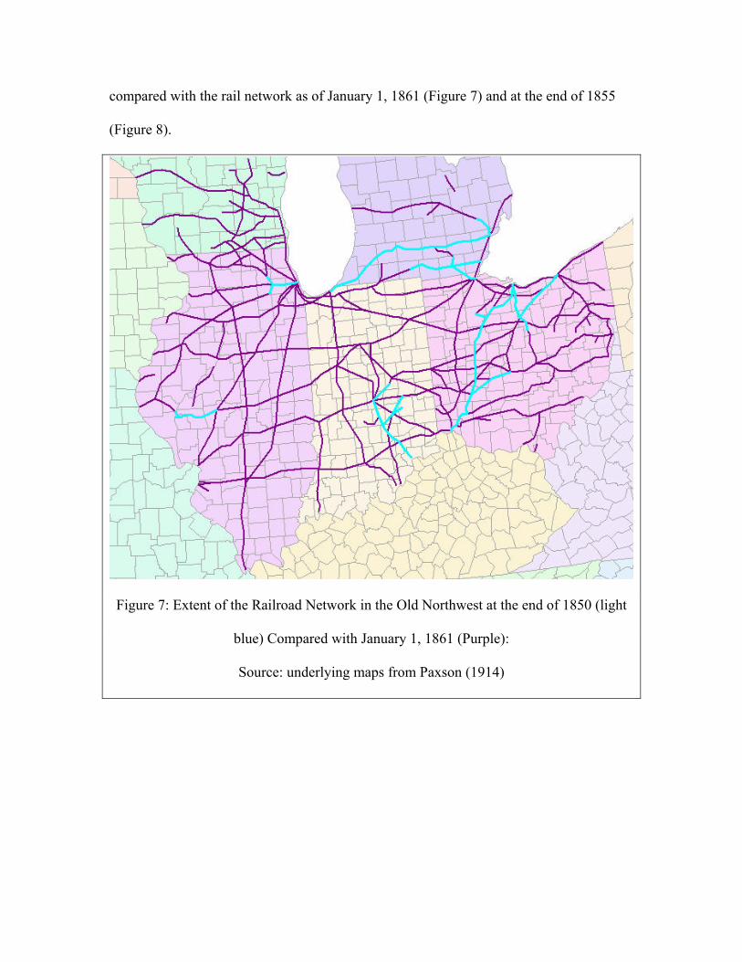
compared with the rail network as of January 1, 1861 (Figure 7) and at the end of 1855

(Figure 8).

Figure 7: Extent of the Railroad Network in the Old Northwest at the end of 1850 (light

blue) Compared with January 1, 1861 (Purple):

Source: underlying maps from Paxson (1914)

Figure 8: Extent of the Railroad Network in the Old Northwest at the end of 1855 (light

blue) Compared with January 1, 1861 (Purple):

Source: underlying maps from Paxson (1914)

Bibliography

(These are in addition to the on-line sources cited in the footnotes)

Bianculli, A. J. (2001). Trains and technology : the American railroad in the nineteenth century. Newark, DE, University of Delaware Press.

Carter, S. B., S. S. Gartner, et al. (2006). Historical Statistics of the United States Millennial Edition Online. New York, Cambridge University Press.

Cobb, C. and R. S. Fisher (1851). American railway guide, and pocket companion for the United States ... together with a complete railway map. New York, Dinsmore.

Craig, L. A., Palmquist., Raymond B., Weiss, Thomas (1998). "Transportation improvements and land values in the antebellum United States: a hedonic approach." Journal of real estate finance and economics 16(2): 173-189.

D. Appleton and Company. Appletons' illustrated railway and steam navigation guide. New York, N.Y., D. Appleton & Co.: v.

Disturnell, J. (1847). Disturnell's guide through the middle, northern, and eastern states containing a description of the principal places, canal, railroad, and steamboat routes, tables of distances, etc. : compiled from authentic sources. New York, J. Disturnell.

Doggett, J. (1848). Doggett's railroad guide and gazetteer for--1848--with sectional maps of the great routes of travel. New York, John Doggett Jr. proprietor 64 Liberty Street. Also for sale by ... 14 others in 12 cities : S.W. Benedict stereotyper and printer 16 Spruce Street.

Fishlow, A. (1965). American railroads and the transformation of the antebellum economy. Cambridge,, Harvard University Press.

Fogel, R. W. (1964). Railroads and American economic growth: essays in econometric history. Baltimore,, Johns Hopkins Press.

Goodrich, C. (1961). Canals and American economic development, y Carter Goodrich [and others]. New York,, Columbia University Press.

Haines, M. R., Margo, Robert A. (2007). Railroads and Local Economic Development: The United States in the 1850s, in. Quantitative Economic History: The Good of Counting. J. Rosenbloom, Routledge.

Jenks, L. H. (1944). "Railroads as an Economic Force in American Development." The Journal of Economic History 4(1): 1-20.

Lloyd, E. (1857). Lloyd's American guide : containing new arranged time tables, so simple and correct that a child can understand them, it being universally acknowledged that all other guide books are so complicated that not one in a hundred can understand them : the population, states, and distances to every place on all the railroad routes in the United States and Canadas : photographic portraits of all the railroad presidents and superintendents--men controlling. Philadelphia, E. Lloyd.

Paxson, F. L. (1914). "The Railroads of the "Old Northwest" before the Civil Wat." Transactions of the Wisconsin Academy of Sciences, Arts, and Letters 17(Part 1): 247-274.

Puffert, D. J. (1991). The economics of spatial network externalities and the dynamics of railway gauge standardization.

Rand McNally and Company., National General Ticket Agents' Association., et al. (1879). The Rand-McNally official railway guide and hand book. Chicago, National Railway Publication Co.

Rothenberg, W. B. (1981). "The Market and Massachusetts Farmers, 1750-1855." The Journal of Economic History 41(2): 283-314.

Schumpeter, J. A. and R. Fels (1964). Business cycles; a theoretical, historical, and statistical analysis of the capitalist process. New York,, McGraw-Hill.

Senate, U. S. C. and U. S. D. o. t. Treasury (1808). Roads and canals. Communicated to the Senate, April 6, 1808.

Taylor, G. R. and I. D. Neu (1956). The American railroad network, 1861-1890. Cambridge,, Harvard University Press.

Vernon, E. and National General Ticket Agents' Association. (1871). Travelers' official railway guide for the United States and Canada, : containing railway time schedules, connections and distances, ocean and inland steam navigation routes, maps of principal lines and lists of general officers, general index of towns and villages on the various railways, (corrected and amended up to date) together with all such miscellaneous information relative to railway improvements and progress as may be useful to the traveling public. Philadelphia, The National Railway Publication Co. publishers and proprietors. No. 237 Dock Street.

Williams, W. and D. Appleton and Company. (1849). Appletons' railroad and steamboat companion : being a travellers' guide through the Northern, Eastern, and middle states, Canada, New Brunswick, and Nova Scotia : forming, likewise, a complete guide to the White Mountains, Catskill Mountains, &c., Niagra Falls, Trenton Falls, &c., Saratoga Springs, Virginia Springs and other watering-places : with the places of fashionable and healthful resort : and containing full and accurate descriptions of the principal cities, towns, and villages, the natural and artificial curiosities in the vicinity of the routes, with distances, fares, &c. : illustrated by 30 maps, engraved on steel, including four plans of cities, and embellished with twenty-six engravings. New York, D. Appleton.