THE TOLERANCE OF WW -IRON MASTER OLDdigital.library.okstate.edu/etd/umi-okstate-2374.pdf · THE...

THE TOLERANCE OF WW-IRON MASTER OLD

WORLD BLUESTEM TO SALINITY AND

LAND-APPLICATION OF

SWINE EFFLUENT

By

SPENCER LEE MANN

Bachelor of Science

Utah State University

Logan, Utah

2005

Submitted to the Faculty ofthe Graduate College of

Oklahoma State Universityin partial fulfillment of

the requirements forthe Degree of

MASTER OF SCIENCEJuly, 2007

ii

THE TOLERANCE OF WW-IRON MASTER OLD

WORLD BLUESTEM TO SALINITY AND

LAND-APPLICATION OF

SWINE EFFLUENT

Thesis Approved:

_______________Michael A. Kizer_______________Thesis Advisor

________________Daren Redfearn_______________

_________________Marvin Stone________________

______________A. Gordon Emsilie______________Dean of the Graduate College

iii

Acknowledgments

This thesis would not have been possible without the support and contributions of

my wife, Cynthia Mann. Her strong back, uncanny ability to find my errors, and strong

desire to live closer to her family qualified her to act as laborer, editor and motivator on

this project.

I extend my thanks to all my committee members, Dr. Michael Kizer, Dr. Daren

Redfearn, and Dr. Marvin Stone. I would particularly like to express my appreciation for

Dr. Kizer who has been a tremendous advisor and friend. Likewise, I am grateful for Dr.

Elliott who believed in me and provided me with the opportunity to earn this degree.

I would also like to acknowledge the enormous contribution to this thesis made by

the cut and paste function of Microsoft “Word” ®, as well as the other editing functions

found on modern computers. My heart goes out to the Old World bluestem plant family

for the losses it suffered as a result of this research. My sympathy is particularly strong

for those unfortunate plants whose noble death resulted from over application of swine

effluent.

Finally, I would like to express my gratitude to my God, by whom all things are

possible.

iv

Table of ContentsChapter Page

I. Introduction............................................................................................................. 1Statement of the Problem.................................................................................. 1Objectives of the Study..................................................................................... 1

II. Literature Review.................................................................................................... 3Water Transport into Roots............................................................................... 6Salinity Effect on Water Transport into Roots ................................................. 9

III. Salt Tolerance of WW-Iron Master Old World Bluestem, Dichanthium spp....... 11Abstract ........................................................................................................... 11Introduction..................................................................................................... 12Material and Methods ..................................................................................... 14Results and Discussion ................................................................................... 16Salt Program Analysis..................................................................................... 16Comparison of Two Models ........................................................................... 19Plant Ion Concentrations................................................................................. 22Conclusion ...................................................................................................... 24References....................................................................................................... 25

IV. Statistical Study of Swine Effluent Application on WW-Iron Master Old WorldBluestem, Dichanthium spp. ................................................................................. 27

Abstract ........................................................................................................... 27Introduction..................................................................................................... 28Material and Methods ..................................................................................... 28Results and Discussion ................................................................................... 36Conclusions..................................................................................................... 37References....................................................................................................... 38

V. Related Experiments ............................................................................................. 39Effluent Application at Farm .......................................................................... 39

Material and Methods ............................................................................ 39Reflectance Index Results...................................................................... 42Dry Weight Results................................................................................ 45Conclusion ............................................................................................. 47

Salt Solution Spray in Greenhouse ................................................................. 49Materials and Methods........................................................................... 49Results and Discussion .......................................................................... 50Conclusion ............................................................................................. 51

Spray in Greenhouse with Quick Dry............................................................. 51Materials and Methods........................................................................... 51Results and Discussion .......................................................................... 52

v

Conclusion ............................................................................................. 53VI. Conclusions........................................................................................................... 54

Recommendations for Future Studies............................................................. 56VII. References............................................................................................................. 58

VIII. Appendices............................................................................................................ 60Appendix A: Relevant Tables and Figures for Hydroponics Salt ToleranceStudy. .............................................................................................................. 61Appendix B: Relevant Tables and Figures for Statistical Study of SwineEffluent Application on Old World Bluestem. ............................................... 69Appendix C: Relevant Tables and Figures for Related Experiments. ........... 74

vi

List of Tables

Table Page

III-a. Treatment preparation values. …………………………………………………...15

III-b. Variable and statistical values for each period as calculated by the SALTprogram using equation 1……………………………………………………….. 17

III-c. Variables used in the piecewise linear response model for each period. ………..20

IV-a. Variables considered for development of unbiased model. ……………………..29

IV-b. Potentially significant variables for development of unbiased model. ………….30

IV-c. Potentially significant variables chosen for development of biased …………….33

IV-d. Comparison of models developed from the two sets of variables. ……………...37

V-a The average initial and final reflectance index for each treatment and theirdifference. ……………………………………………………………………….43

V-b The average difference in reflectance index for each treatment afterapplication. ……………………………………………………………………....43

V-c The average total dry weight of each treatment. ………………………………...45

V-d Summary of the effects of the time of application. ………………………..…….48

vii

List of Figures

Figure Page

II-a. The two most common methods of water transport into a root…………………...7

III-a. Photo of actual experiment setup………………………………………………...14

III -b. Photo of final effect of salt solution……………………………………………...16

III -c. Percent shoot growth for the first two-week period as influenced bysalinity…………………………………………………………………………....18

III -d. Percent shoot growth for the second two-week period as influenced bysalinity…………………………………………………………………………....18

III -e. Percent shoot growth for the third two-week period as influenced bysalinity…………………………………………………………………………....19

III -f. Percent shoot growth for the fourth two-week period as influenced bysalinity…………………………………………………………………………....19

III -g. Comparison of curves generated by the salt program and the piecewiselinear response model for the first two-week period as influenced by salinity….20

III -h. Comparison of curves generated by the salt program and the piecewiselinear response model for the second two-week period as influenced bysalinity……………………………………………………………………………21

III -i. Comparison of curves generated by the salt program and the piecewiselinear response model for the third two-week period as influenced bysalinity……………………………………………………………………………21

III -j. Comparison of curves generated by the salt program and the piecewiselinear response model for the fourth two-week period as influenced bysalinity……………………………………………………………………………22

III -k. Comparison between percent dry mass Na+ composition of the shootsand roots as influenced by salinity…………………………………………….…23

viii

III-l. Comparison of the percent dry mass Na+ and K+ composition in the rootsas influenced by salinity……………………………………………………….…24

III-m. Comparison of the percent dry mass Na+ and K+ composition in the shootsas influenced by salinity……………………………………………………….…24

V-a. Plot layout design………………………………………………………………...39

V-b. Application apparatus……………………………………………………………41

V-c. Photo of actual apparatus in field………………………………………………...41

V-d. Harvest of treated stands one month after application…………………………...42

V-e. The average difference in reflectance index for each treatment afterapplication………………………………………………………………………..44

V-f. The average total dry weight of each treatment………………………………….46

V-g. Graphical comparison of application time effect. Percent effect is thepercent of the maximum observed effect of its type each represented…………..48

V-h. Summary of the effect of salinity on the change in reflectance index…..……….50

V-i. Summary of the effect of salinity on the change in reflectance index..………….52

1

Chapter I

Introduction

Statement of the Problem

A sizable portion of grassland in western Oklahoma and northwest Texas was

seeded with WW-Iron Master Old World bluestems in the Conservation Reserve Program

(CRP) (Harmoney and Hickman, 2004). However, the growing swine industry in the

western parts of Oklahoma has found that Old World bluestems are sensitive to swine

effluent application. A portion of this sensitivity may be the result of salt burns, likely

chloride or sodium, left on foliage when swine effluent is applied during warm days with

high solar radiation. Unfortunately, no information regarding the salinity tolerance of

these grasses, or their potential for salt burns during effluent application exists in

scientific literature. Information in this domain could improve grassland management

and fill the existing gap in our understanding of the salinity tolerance of WW-Iron Master

Old World bluestems.

Objectives of the Study

The objectives of this study are to:

1. Determine the salinity tolerance threshold for WW-Iron Master Old World

bluestem;

2. Determine the fractional yield decline per unit increase in salinity beyond the

threshold;

2

3. Determine if the time of day the effluent is applied to the plant has a significant

effect on plant growth;

4. Determine the optimum dilutions for swine effluent when applied to WW-Iron

Master Old World bluestem;

5. Verify that using the “Greenseeker” is an adequate method for determining

salinity effects on plant growth;

6. Determine if a salt solution spray on foliage can cause plant damage;

7. Determine if foliage burn during swine effluent application is a result of chemical

constituents other than salts; and to

8. Statistically evaluate effluent application data from the Conservation Reserve

Program gathered from 1999-2005 by the Farm Service Agency.

3

Chapter II

Literature Review

Salinity is a significant factor for affecting plant growth in arid climates. For

many plants, the values of salt tolerance and the fractional yield decline per unit increase

in salinity are already known (Hoffman et al., 1980). However, salinity tolerance values

for Old World bluestems, a group of grasses commonly grown for forage, have not been

published.

Old World bluestems, which originate from Russia and surrounding Asian

countries, were introduced into the United States around 1920. They are warm-season

perennial bunchgrasses that are best adapted to loam or clay-loam soils (Redfearn, 2004).

Old World bluestems begin growth during late spring and perform better during the hot

parts of summer than other warm-season grasses. Old World bluestems are generally

dormant from mid-September to mid-May (Bell and Caudle, 1994). However, because

Old World bluestem is more receptive to late summer precipitation than other warm-

season grasses, it can still experience significant growth in August and September.

There are many cultivars of Old World bluestems, with the most common being

‘Caucasian’, ‘Ganada’, ‘King Ranch’, ‘Plains’, ‘WW-Spar’, ‘WW-Iron Master’ and

‘WW-B Dahl’. Despite an increased tolerance for iron deficient soils, WW-Iron Master

is a fairly representative variety of Old World bluestems (Redfearn, 2004).

To determine salt tolerance, a hydroponics solution is generally used to control

nutrient availability. Because soil is not used, researchers can accurately test plant

4

response to nutrient solutions. Consequently, hydroponics is ideal for salt tolerance

determination. For plant growth it is essential that the nutrient solution contain relatively

large concentrations of nitrogen, potassium, phosphorus, calcium, magnesium and sulfur,

with smaller concentrations of iron, manganese, boron, zinc, and copper. Hydroponic

solutions can be created from the formula developed by Dr. D.R. Hoagland (Jones, 1997;

Hoagland and Arnon, 1950). However, quality solutions based on Dr. Hoagland’s

formula can be purchased commercially and still yield excellent results (Hydroponics as a

Hobby, 2006).

Understanding how environmental conditions can affect water transport in plants

has vast agricultural implications. This is particularly true in waste management

applications. While extreme care is taken to ensure that land application of waste does

not exceed nitrogen and phosphorous limits for crops, the effluent effect on the soil

salinity is often overlooked. Our ability to apply animal waste to agricultural land in a

sustainable manner is dependent on our understanding of the possible effects this salinity

may have on plant growth.

Manure application on a crop can be accomplished through a variety of methods:

1) manure can be applied to ground before seeding; 2) topdressed over established stands;

3) flood applied to established stands; 4) applied after harvest. In the case of manure

application on existing stands of Old World bluestem, some methods are better than

others (Kelling, and Schmitt, 2003).

Application of manure before stand establishment is limited in scope. Perennial

grasses like Old World bluestem are planted once and then maintained year after year for

5

forage. While this method of application has been shown to significantly increase harvest

yields, it is only applicable during planting (Kelling, and Schmitt, 2003).

The most common form of manure application to established stands of forage is

topdress. This method is inherently dangerous to plant growth because it can damage

plant crowns, result in runoff, and in some cases cause salt burn on forage material.

Because swine effluent has a high salt concentration, topdress application must be done

carefully to avoid salt burn. The burn potential of manure is directly related to its

ammonium N and salt concentrations (Kelling, and Schmitt, 2003).

Flood application of effluent avoids some problems associated with topdress

application but creates new difficulties. Physical damage to plant crowns and salt burns

may be prevented through flood irrigation. However, these benefits are offset by the

potential for uneven application and excessive runoff. Additionally, the topography of

the land will likely make flood application impossible.

Finally, a topdressing application after harvest may be the most practical

approach. Soon after a harvest the vegetated canopy of a plant will be limited and

consequently its potential for salt burn will be minimized. However, factors such as

runoff and crown damage are still present (Kelling, and Schmitt, 2003).

Water Transport into Roots and the Effect of Salinity

Water transport into roots is crucial to plant growth. Although the principle of

water transport from a soil into a root is simple, the mechanisms are complicated and not

completely understood. Mathematical models describing water and nutrient transport

through a root have consistently been altered and revised as researchers have made new

6

discoveries. However, the significant discovery of parallel pathways of water transport

has lead to an improved understanding of root-soil interaction.

Understanding how environmental conditions can affect water transport into

plants has vast agricultural implications. This is particularly true in waste management


not exceed nitrogen and phosphorous limits for crops, the effluent’s effect on the soil

salinity is often overlooked. Our ability to effectively apply animal waste to forage is

dependent on our understanding of the possible effects this salinity may have on plant

growth.

Water Transport into Roots

There are many mechanisms by which water enters a plant through the root.

Traditionally, water was assumed to only move radially through the root via the apoplast

as shown in Figure II-a. It was thought that water moved around the outside of the

protoplasts because they posed a greater hydraulic resistance than found in the apoplast.

As water reaches the endodermis of the root, the Casparian band prevents further apoplast

water movement. At this point water is transferred across the endodermis cell membrane

and then out again into the xylem vessels located at the center of the root. However

research has shown that there is a strong argument for an alternative method of water

transport. This alternative route, known as the symplastic route, involves water entering

plant cell membranes, traversing the cell and passing out again to enter the next cell as

shown in Figure II-a (Cummings, 2006). Both the apoplastic and symplastic routes end

in the water entering the xylem vessels where horizontal water transportation takes place.

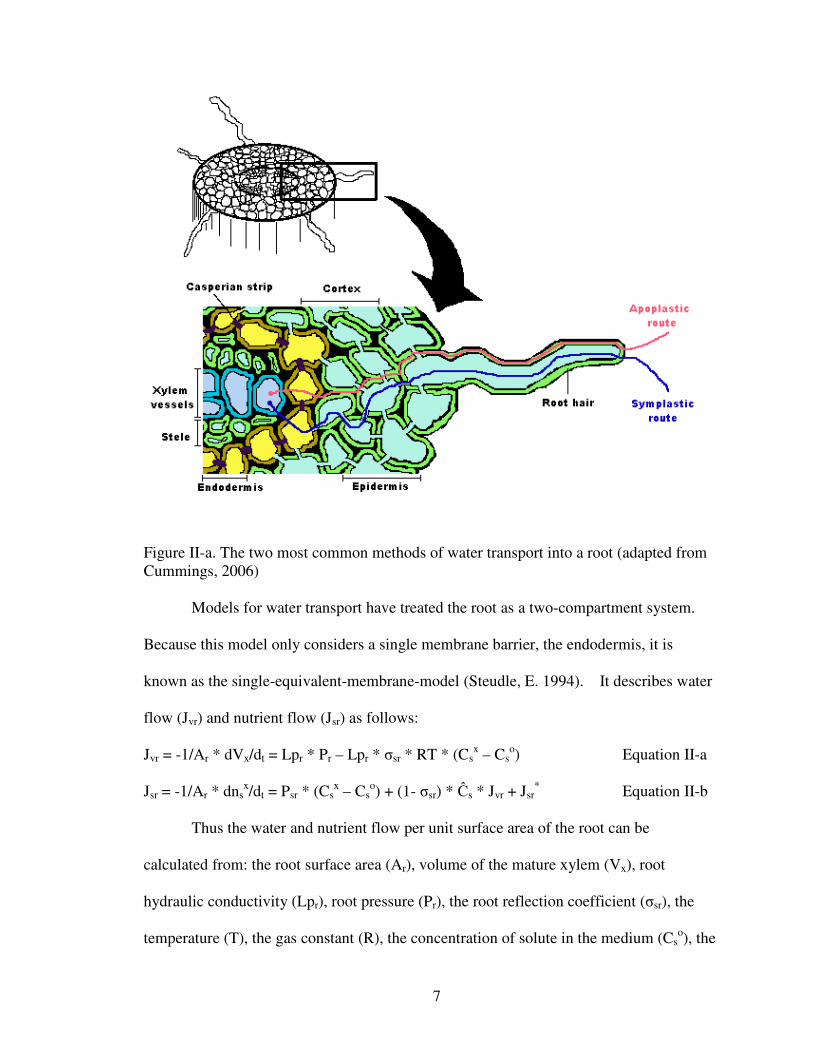
7

Figure II-a. The two most common methods of water transport into a root (adapted fromCummings, 2006)

Models for water transport have treated the root as a two-compartment system.

Because this model only considers a single membrane barrier, the endodermis, it is

known as the single-equivalent-membrane-model (Steudle, E. 1994). It describes water

flow (Jvr) and nutrient flow (Jsr) as follows:

Jvr = -1/Ar * dVx/dt = Lpr * Pr – Lpr * σsr * RT * (Csx – Cs

o) Equation II-a

Jsr = -1/Ar * dnsx/dt = Psr * (Cs

x – Cso) + (1- σsr) * Ĉs * Jvr + Jsr

* Equation II-b

Thus the water and nutrient flow per unit surface area of the root can be

calculated from: the root surface area (Ar), volume of the mature xylem (Vx), root

hydraulic conductivity (Lpr), root pressure (Pr), the root reflection coefficient (σsr), the

temperature (T), the gas constant (R), the concentration of solute in the medium (Cso), the

8

concentration of solute in the xylem (Csx), the amount of solute in the xylem (ns

x), the

permeability coefficient of the root (Psr), the mean concentration of solute in the root (Ĉs

= (Csx + Cs

o)/2), and the active solute flow (Jsr*). Unlike previous models, these

equations account for the alternative mechanisms of water transport. These alternative

mechanisms are the passive transport of a solute across the root according to Fick’s Law,

and active transport of solute into the root through metabolism (Steudle, 1994).

However, experimental research shows deviation from the single-membrane-

equivalent model. This deviation is a result of the incorrect assumption that water travels

radially through a root via a single pathway. In truth, water enters the root through two

parallel pathways, as mentioned earlier. To correct for parallel pathways, the new

composite-transport-model of the root is used (Steudle, 1994). The composite pathway

uses the equation established in the single-equivalent-membrane-model (Equations II-a

and II-b) but adjusts the overall reflection coefficient (σsr) to correct for the alternative

pathways. The corrected overall reflection coefficient is:

σsr = γcc * Lpcc/Lpr * σscc + γcw * Lpcw/Lpr * σs

cw Equation II-c

Where Lpr is the overall hydraulic conductivity, Lpcc is the hydraulic conductivity

of the cell-to-cell and Lpcw is the hydraulic conductivity of the apoplasmic pathway.

Additionally, γcc and γcw are the fractional contributions of cross sectional areas of

pathways to the overall root area (Steudle, 1994).

When the soil a plant is growing in becomes so dry that its water potential is less

than the roots, water flow into the plant generally stops. To prevent reverse water flow

during long dry periods the roots will suberize. Suberization is the deposition of a

waterproof wax substance on the walls of plant cells to inhibit water flow. Renewed

9

permeability of plant roots after suberization generally takes several days (Passioura,

1988).

Salinity Effect on Water Transport into Roots

Although it is well known that salinity has a detrimental effect on plant growth,

the mechanisms of this inhibition remain a mystery. Additionally, the physiological

differences between a salt tolerant and a salt sensitive plant are not completely

understood. However, new research has produced evidence which indicates that salt

tolerance is generally a result of one of two mechanisms. These mechanisms are first:

transport and control of salt before and after entering the plant; and second: adjustment of

other metabolic activities to adjust for the increased salinity (Cheeseman, 1988).

Most research on salt tolerance has focused on the transmembrane movement

found in the roots. In the root tissue, a plant’s tactic for accommodating high saline

conditions generally designates it as a salt includer or salt excluder. A salt includer will

allow salt to enter the roots and use it to create osmotic pressure, while a salt excluder

will prevent salt from entering the roots. As salt levels inside the plant increase, some

plants will store high saline solution in internal pools which are periodically emptied

outside the root. Because of enzyme sensitivity, salts must be excluded from the

cytoplasm. To protect the enzymes, salts are compartamentalized inside the cell.

Additionally, plants have shown control over nutrient balances between the root and

shoots. Consequently, it is reasonable to assume that plants possess the means to

maintain normal salt concentrations in the shoots while still accumulating salt in the roots

(Cheeseman, 1988).

10

The necessary metabolic adjustments a plant makes primarily involve its use of

carbon. Carbon availability is the determinant for plant growth, energy storage, nutrient

transport and cellular maintenance. High salinity’s increased demands on cellular

maintenance and nutrient transport have significant effects on carbon availability. As

carbon levels drop, plant growth decreases significantly (Cheeseman, 1988).

According to O’Leary, the growth inhibition a plant growing in a saline solution

experiences is not caused by physiological drought. Although the osmotic pressure in the

root has been shown to increase with soil salinity, this does not necessarily mean that the

plant is not reacting as it would to a drought. As the research by Cheeseman has shown,

plant roots and shoots have specific reactions to saline conditions. Consequently, plant

roots may prevent water from reaching shoots and the leaves will in fact experience a

physiological drought while the roots will not. This reaction is favorable since it

decreases water transpiration and allows the plant to better survive poor environmental

conditions (O'Leary. J, 1969; Cheeseman, 1988).

11

Chapter III

Salt Tolerance of WW-Iron Master Old World Bluestem, Dichanthium spp.

By S. L. Mann, M. Kizer and D. Redfearn

Department of Biosystems and Agricultural Engineering, Oklahoma State University,

Stillwater Oklahoma

Abstract

Stands of Old World bluestem (Dichanthium spp.) are grown extensively in the Southern

Great Plains. Swine production facilities have also increased significantly in this region.

In some cases, swine effluent application on these stands has resulted in total stand loss.

High salinity sensitivity of Old World bluestem was suspected as the cause and this study

was conducted to determine its salinity sensitivity. WW-Iron Master Old World

bluestem response in both shoot and root growth under various saline conditions was

studied. Old World bluestem was grown in a greenhouse in hydroponic media at 1, 2, 3

5, 10, 20, and 30 dS/m (0, 19, 29, 49, 99, 198, and 298 mM NaCl) and was replicated

four times. Shoot growth was harvested every fourteen days. With each successive

harvest the effects of the saline solution on plant growth became more pronounced. This

indicates that the effects of salinity on the growth of the Old World bluestem plant

growth have a cumulative effect. After twenty eight days the effect of salinity on plant

growth reached a steady state. The salinity threshold for Old World bluestem was found

using the piecewise linear response model to be 1 ds/m and the fractional yield decline

per unit increase in salinity beyond the threshold was 21 %. Additionally, the Na+

12

accumulation in the shoots was much greater than the root tissue, indicating that Old

World bluestem is unable to restrict Na+ transport.

Introduction

Salinity is a significant factor for affecting plant growth in arid climates. For

many plants, the values of salt tolerance and the fractional yield decline per unit increase

in salinity are already known (Hoffman et al., 1980). However, salinity tolerance values

for Old World bluestems, a group of grasses commonly grown for forage, have not been

published.



perennial bunchgrasses that are best adapted to loam or clay-loam soils (Redfearn, 2004).

Old World bluestems begin growth during late spring and perform better during the hot

parts of summer than other warm-season grasses. Old World bluestems are generally

dormant from mid-September to mid-May (Bell and Caudle, 1994). However, because

Old World bluestem is more receptive to late summer precipitation than other warm-

season grasses, it can still experience significant growth in August and September.

It is a common practice to use swine lagoon effluent for irrigation in the

production of forages. Proper application of swine effluent requires careful analysis of

the effluent constituents, the soil properties and the nutrient needs of the intended forage.

Although nitrogen is the primary element in application analysis, other elements such as

phosphorous, copper and zinc are also important to consider.

The Conservation Reserve Program (CRP) is a federal government program

designed to help restore wildlife habitat, protect topsoil from erosion, and reduce water

13

runoff and sedimentation. In locations where CRP land is near animal production

facilities it is not uncommon for effluent from animal waste lagoons to be applied on

CRP soil.

To determine salt tolerance, a hydroponics solution is generally used to control

nutrient availability. Because soil is not used, researchers can accurately test plant

response to nutrient solutions. Consequently, hydroponics is ideal for salt tolerance

determination. For plant growth it is essential that the nutrient solution contain relatively

large concentrations of nitrogen, potassium, phosphorus, calcium, magnesium and sulfur,

with smaller concentrations of iron, manganese, boron, zinc, and copper. Hydroponic

solutions can be created from the formula developed by Dr. D.R. Hoagland (Jones, 1997;

Hoagland and Arnon, 1950). However, quality solutions based on Dr. Hoagland’s

formula can be purchased commercially and still yield excellent results (Hydroponics as a

Hobby, 2006).

Understanding how environmental conditions can affect water transport in plants

has vast agricultural implications. This is particularly true in waste management


not exceed nitrogen and phosphorous limits for crops, the effluent effect on the soil

salinity is often overlooked. Our ability to apply animal waste to agricultural land in a

sustainable manner is dependent on our understanding of the possible effects this salinity

may have on plant growth.

14

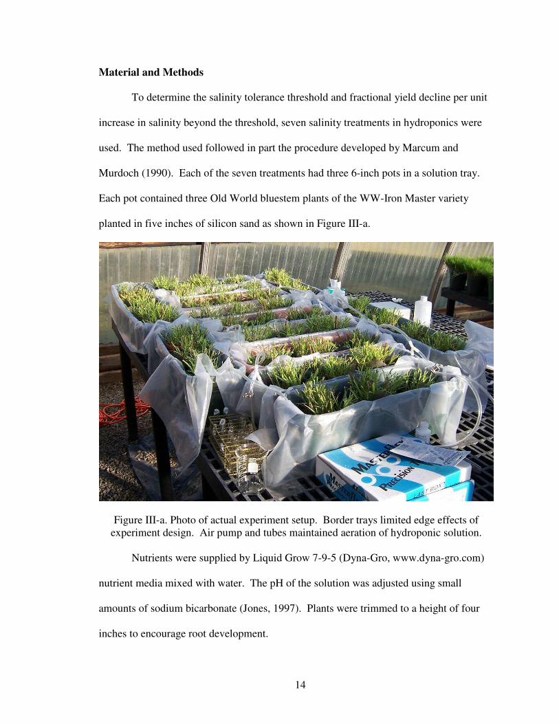
Material and Methods

To determine the salinity tolerance threshold and fractional yield decline per unit

increase in salinity beyond the threshold, seven salinity treatments in hydroponics were

used. The method used followed in part the procedure developed by Marcum and

Murdoch (1990). Each of the seven treatments had three 6-inch pots in a solution tray.

Each pot contained three Old World bluestem plants of the WW-Iron Master variety

planted in five inches of silicon sand as shown in Figure III-a.

Figure III-a. Photo of actual experiment setup. Border trays limited edge effects ofexperiment design. Air pump and tubes maintained aeration of hydroponic solution.

Nutrients were supplied by Liquid Grow 7-9-5 (Dyna-Gro, www.dyna-gro.com)

nutrient media mixed with water. The pH of the solution was adjusted using small

amounts of sodium bicarbonate (Jones, 1997). Plants were trimmed to a height of four

inches to encourage root development.

15

Salinity treatments began after plants were given 30 days to become established in

the pots (Francois et al., 1990). Salinity treatments of 1, 2, 3, 5, 10, 20 and 30 ds/m (0,

19, 29, 49, 99, 198, and 298 mM NaCl) were used. Salinity levels for each treatment

increased 2.8 g NaCl/liter every two days until the desired salinity was attained, see Table

III-a. Every other day water purified by reverse osmosis was added to the solution trays

to maintain 2 inches of media in the trays. Additionally, the media was drained and

replaced with fresh media each week. Aeration was supplied both by the sand bedding

and a tube network connected to an aquarium pump (Taliaferro et al., 1995; Marcum and

Murdoch, 1990; Lee et al., 2005).

dS/mmM

NaCLg

NaCl/LDays

Required1 0 0.0 02 19 1.1 03 29 1.7 05 49 2.8 010 99 5.6 220 198 11.2 630 298 16.8 10

Table III-a. Treatment preparation values.

When each of the desired salinity levels were reached the plant shoots were

trimmed to a height of four inches. Every 2 weeks shoots were clipped for dry weight

determination. All plant material was then dried at 70o C for 48 hrs (Marcum and

Murdoch, 1990). This process continued for 4 harvests. After the final harvest, each of

the plants was carefully removed from the sand bedding. Shoot and root samples were

obtained from each treatment and tested for concentrations of Na+ and K+.

Data were then analyzed by the SALT program developed by van Genuchten and

Hoffman (1980).

16

Results and Discussion

The effects of salinity on plant growth became more pronounced with time.

Plants grown in a saline solution of 30 ds/m required two weeks before growth was

stopped, while plants grown in 20 ds/m required four weeks before growth stopped.

However, the effect of the saline media on plant growth seemed to stabilize after 6

weeks. The final effect of the salt solution can be seen in Figure III-b.

Figure III-b. Photo of final effect of salt solution. The photo shows the effect of eachtreatment starting with pure water (the tray missing one pot) and moving with increasing

salinity to 30 ds/m (the second furthest tray in the middle).

Salt Program Analysis

The salt program developed by van Genuchten and Hoffman (1980) was used to

analyze the data. The data best-fit Equation III-a and the SALT program calculated

values for Ym, C50 and P which would provide the lowest sum of squares residual for the

data. Where Ym is the yield under non-saline conditions, C50 is the salinity at which yield

17

is reduced by 50%, p is an empirical constant, C is the salinity of the soil and Y is the

expected dry mass in grams of plant growth at C (van Genuchten and Hoffman, 1980).

Again, because of the cumulative effect of salinity on plant growth, the values for these

variables changed with time. However, the curves for the third two-week period and the

fourth two-week period are very similar. The variable values calculated by the SALT

program for each period are shown in Table III-b. Additionally, the r2 and RMSE values

for the fitted curves in transformed space are also show in Table III-b; no trend was found

in the plotted residuals.

Y = Ym/[1+(C/C50)p] Equation III-a

Variable Days 0-14 Days 14-28 Days 28-42 Days 42-56 Ym 0.20 0.12 0.13 0.21C50 7.30 7.51 3.74 2.75P 1.38 3.23 3.42 2.97r2 0.32 0.54 0.76 0.81

RMSE 0.15 0.15 0.11 0.10

Table III-b. Variable and statistical values for each period as calculated by theSALT program using equation 1.

The fitted curves and data points as a percent of maximum growth for these four

periods are shown in Figures III-c through III-f. The data in the figures are compared to

the 100% maximum growth, which is the mean growth of plants grown without salt

added to hydroponics solution.

18

Days 0-14

0%

50%

100%

150%

200%

250%

300%

0 5 10 15 20 25 30 35

Salinity (ds/m)

%M

axim

um

Gro

wth

Data Fitted Curve

Figure III-c. Percent shoot growth for the first two-week period as influenced by salinity.

Days 14-28

0%

50%

100%

150%

200%

250%

300%

0 5 10 15 20 25 30 35

Salinity (ds/m)

%M

axim

um

Gro

wth

Data Fitted Curve

Figure III-d. Percent shoot growth for the second two-week period as influenced bysalinity. (2 data points representing individual plants which grew more than 300% are not

shown on graph.)

19

Days 28-42

0%

50%

100%

150%

200%

250%

300%

0 5 10 15 20 25 30 35

Salinity (ds/m)

%M

axim

um

Gro

wth

Data Fitted Curve

Figure III-e. Percent shoot growth for the third two-week period as influenced by salinity.

Days 42-56

0%

50%

100%

150%

200%

250%

300%

0 5 10 15 20 25 30 35

Salinity (ds/m)

%M

axim

um

Gro

wth

Data Fitted Curve

Figure III-f. Percent shoot growth for the fourth two-week period as influenced bysalinity.

Comparison of Two Models

The data were also analyzed using the piecewise linear response model and

compared against the fitted curves from the salt program (Figures III-g to III-j). For these

comparisons, a single mean value of the nine replications was calculated for each of the

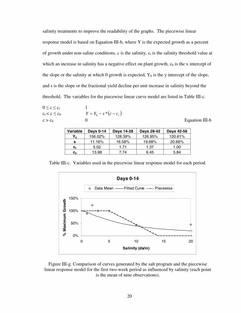
20

salinity treatments to improve the readability of the graphs. The piecewise linear

response model is based on Equation III-b, where Y is the expected growth as a percent

of growth under non-saline conditions, c is the salinity, ct is the salinity threshold value at

which an increase in salinity has a negative effect on plant growth, c0 is the x intercept of

the slope or the salinity at which 0 growth is expected, Y0 is the y intercept of the slope,

and s is the slope or the fractional yield decline per unit increase in salinity beyond the

threshold. The variables for the piecewise linear curve model are listed in Table III-c.

0 ≤ c ≤ ct 1ct < c ≤ c0 ( )tccsYY −−= *0

c > c0 0 Equation III-b

Variable Days 0-14 Days 14-28 Days 28-42 Days 42-56 Y0 156.02% 128.39% 126.95% 120.61%s 11.16% 16.58% 19.68% 20.66%ct 5.02 1.71 1.37 1.00c0 13.98 7.74 6.45 5.84

Table III-c. Variables used in the piecewise linear response model for each period.

Days 0-14

0%

50%

100%

150%

0 5 10 15 20

Salinity (ds/m)

%M

axim

um

Gro

wth

Data Mean Fitted Curve Piecewise

Figure III-g. Comparison of curves generated by the salt program and the piecewiselinear response model for the first two-week period as influenced by salinity (each point

is the mean of nine observations).

21

Days 14-28

0%

50%

100%

150%

0 5 10 15 20

Salinity (ds/m)

%M

axim

um

Gro

wth


Figure III-h. Comparison of curves generated by the salt program and the piecewiselinear response model for the second two-week period as influenced by salinity (each

point is the mean of nine observations).

Days 28-42

0%

50%

100%

150%

0 5 10 15 20

Salinity (ds/m)

%M

axim

um

Gro

wth


Figure III-i. Comparison of curves generated by the salt program and the piecewise linearresponse model for the third two-week period as influenced by salinity (each point is the

mean of nine observations).

22

Days 42-56

0%

50%

100%

150%

0 5 10 15 20

Salinity (ds/m)

%M

axim

um

Gro

wth


Figure III-j. Comparison of curves generated by the salt program and the piecewise linearresponse model for the fourth two-week period as influenced by salinity (each point is the

mean of nine observations).

Plant Ion Concentrations

At the end of the fourth growth period, samples of plant shoots and roots were

analyzed for Na+ and K+ concentration in the tissue. As shown in Figure III-k, the Na+

concentration in the plant roots and shoots increased linearly with the increasing salinity

of the media. However, the root tissue maintained a much lower Na+ concentration than

was found in the shoots. This indicates that Old World bluestem is incapable of

restricting Na+ from accumulating in the shoots, and is likely the cause of this plant’s

poor salinity tolerance.

23

Percent Na in Plant

y = 0.3192x - 0.1025

R2 = 0.9863

y = 0.0725x + 0.4355

R2 = 0.9697

0

2

4

6

8

10

0 5 10 15 20 25 30Salinity (ds/m)

%N

ao

fT

ota

lMas

s

Shoot Root Linear (Shoot) Linear (Root )

Figure III-k. Comparison between percent dry mass Na+ composition of the shoots androots as influenced by salinity.

As shown in Figure III-l, the concentration of K+ was inversely proportionate to

the Na+ concentration in the root tissue. Many plants selectively uptake K+ while

restricting Na+ uptake to handle saline growing conditions. In this case where the results

indicate that the plant is unable to restrict salt uptake, the decrease in K+ may be caused

by a variety of factors. The increased concentration of Na+ may make passive transport

of K+ impossible, while the remaining K+ is slowly depleted with time. It is also possible

that the plant depletes K+ concentrations to offset the negative effects of saline growing

conditions. However, there was very little effect of salinity on the K+ levels in the shoots

as shown in Figure III-m. This seems to indicate that the strong interaction between Na+

and K+ occurs only in the root tissue.

24

Percent Na and K in Roots

y = 0.0725x + 0.4355

R2 = 0.9697

y = -0.0421x + 1.4535

R2 = 0.8778

0

0.5

1

1.5

2

2.5

3

0 5 10 15 20 25 30Salinity (ds/m)

%N

ao

fT

ota

lM

ass

% K % Na Linear (% Na) Linear (% K)

Figure III-l. Comparison of the percent dry mass Na+ and K+ composition in the roots asinfluenced by salinity.

Percent Na and K in Shoots

y = 0.3192x - 0.1025

R2 = 0.9863

y = -0.0086x + 1.3858

R2 = 0.0739

0123456789

10

0 5 10 15 20 25 30Salinity (ds/m)

%N

ao

fT

ota

lM

ass

% K % Na Linear (% Na) Linear (% K)

Figure III-m. Comparison of the percent dry mass Na+ and K+ composition in the shootsas influenced by salinity.

Conclusion

This research indicates that the effect of salinity on growth of WW-Iron Master

Old World bluestem has a cumulative effect. Following forty two days the effect of

25

salinity on plant growth reached a steady state and the salinity threshold for WW-Iron

Master Old World bluestem was found using the piecewise linear response model to be 1

ds/m and the fractional yield decline per unit increase in salinity beyond the threshold

was 21%. Both the piecewise linear response model and the salt program provided

similar interpretations of the data. However, the piecewise linear response model may be

considered superior because it is easier to interpret.

The mineral analyses of the root and shoot portions of the studied plants

indicated an interaction between K+ and Na+ concentrations in the root tissue of WW-Iron

Master Old World bluestem. With successively higher salinity treatments the increases

in Na+ were matched with decreases in K+. However, the salinity treatment showed no

effect on the K+ concentration in the shoots. Because the Na+ accumulation in the shoot

tissue was much greater than in the root tissue it is concluded that WW-Iron Master Old

World bluestem lacks the mechanisms necessary to restrict Na+ transport to the shoots,

which is likely the cause of its low salt tolerance.

References

Bell, J.R., D.M. Caudle. 1994, June. Range, Wildlife and Fisheries Management.Management of Old World Bluestems. Retrieved December 1, 2006, from:http://www.rw.ttu.edu/newsletter/mgmtnotes.htm

Conservation Reserve Program (n.d.). Retrieved June 4, 2007, fromhttp://www.nrcs.usda.gov/programs/crp/

Francois, L.E., T.J. Donovan, and E.V. Maas. 1990. Salt tolerance of Kenaf. p. 300-301.In: J. Janick and J.E. Simon (eds.), Advances in new crops. Timber Press, Portland, OR.

Hoffman, G.J., R.S. Ayers, E.J. Doering and B.L. McNeal. 1980. Salinity in IrrigatedAgriculture. In: Design and Operation of Farm Irrigation Systems. M.E. Jensen, Editor.ASAE Monograph No. 3. St. Joseph, MI. 829pp.

26

Hoagland, D.R. and Arnon, D.I. (1950). The water-culture method for growing plantswithout soil. California Agricultural Experiment Station Circular 347.

Hydroponics As A Hobby Retrieved September 6, 2006, fromhttp://plantanswers.tamu.edu/publications/hydroponics.html

Jones, J. B. 1997. Hydroponics, a practical guide for the soilless grower. St. Lucie Press,Boca Raton, FL 33431. 230 pp.

Lee G., R. N. Carrow, and R. R. Duncan. 2005. Criteria for Assessing Salinity Toleranceof the Halophytic Turfgrass Seashore Paspalum. Crop Sci., January 1, 2005; 45(1): 251 -258.

Marcum, K.B. and Murdoch, C.L. 1990. Growth responses, ion relations, and osmoticadaptations of eleven C4 Turfgrasses to salinity. Agronomy Journal 82: 892–896.

Redfearn, D.D. 2004. Production and management of old world bluestems. OklahomaCooperative Extension Service, Oklahoma State University Extension Facts, No. 3020(revised).

Taliaferro, C.M., T. Liranso, F.T. McCollum, D.R. Gill, and L.L. Ebro. 1995. Evaluationof ‘World Feeder’ and ‘Gordon’s Gift’ Bermudagrasses Oklahoma Center ForAdvancement of Science and Technology

Van Genuchten, M.T. and Hoffman, G.J. 1984. Analysis of crop salt tolerance data. In:Soil Salinity under Irrigation. Processes and Management. Ecological Studies No. 51,pp: 130-142. Edited by I. Shainberg and J. Shalhevet, Springer-Verlag.

27

Chapter IV

Statistical Study of Swine Effluent Application on WW-Iron Master Old WorldBluestem, Dichanthium spp.

By S. L. Mann, M. Kizer and D. Redfearn

Department of Biosystems and Agricultural Engineering, Oklahoma State University,

Stillwater Oklahoma

Abstract

Stands of Old World bluestem (Dichanthium spp.) are grown extensively in the Southern

Great Plains. Swine production facilities have also increased significantly in this region.

In some cases, swine effluent application on these stands has resulted in total stand loss.

Stand loss may be a consequence of high soil salinity or salt burn on the foliage.

Accumulated salts, generally chloride and sodium left on foliage after swine effluent

application, can be absorbed into the plant and cause foliage damage. Salt burn effects

appear to be most pronounced when application takes place by slowly rotating sprinklers

during warm windy days with low humidity. For this study a statistical analysis was

conducted on seven years of swine effluent application data on to CRP (Conservation

Reserve Program) land in the Goodwell, Oklahoma area. This statistical approach

considered 55 variables for 25 effluent application dates. The analysis indicated that with

an alpha value of 10% there is statistical evidence that soil levels of both NO3-N (lbs/A)

and Cu (mg/l) are significantly correlated with stand loss for swine effluent application

on stands of WW-Iron Master Old World bluestem.

28

Introduction



perennial bunchgrasses that are adapted to a wide range of soil types (Harmoney and

Hickman, 2004). Old World bluestems begin growth during late spring and perform

better during the hot parts of summer than other warm-season grasses. Old World

bluestems are generally dormant from mid-September to mid-May (Bell and Caudle,

1994). Because Old World bluestem is more receptive to late summer rain than other

warm-season grasses, it can still experience significant growth in August and September.

There are many cultivars of Old World bluestems, with the most common being

‘Caucasian’, ‘Ganada’, ‘King Ranch’, ‘Plains’, ‘WW-Spar’, ‘WW-Iron Master’ and

‘WW-B Dahl’. Despite an increased tolerance for iron deficient soils, WW-Iron Master

is a fairly representative variety of Old World bluestems (Redfearn, 2004).

Details on salt burn effects on plants are difficult to obtain because of the strong

environmental influence on the results. Factors that have been shown to contribute to salt

burn are air temperature, wind speed, sprinkler rotation speed, and droplet size (Ayers

and Westcot, 1985). Additionally, plants with high sensitivity to salinity in soil have

been shown to be particularly sensitive to foliar absorption of salts (Maas, 1984).


Preliminary analysis of raw CRP effluent application data required some

assumptions. These assumptions were:

1. Effluent application stopped when stand suffered loss;

2. Stand loss is either complete or non-existent after each application;

29

3. Effluent application took 2 weeks;

4. Rainfall data were only significant during application, one week before, and one

week after;

5. Soil samples and lagoon samples were representative;

6. Effluent application was uniform throughout the field;

7. Application took place during the day; and

8. Weather conditions in Goodwell, Oklahoma represented conditions at all sites.

From May 11, 1999 to July 21, 2005, details of 25 CRP grassland effluent

applications were collected. Based on previously stated assumptions, all consistently

measured independent variables were input into a Microsoft Excel ® spreadsheet. This

set of independent variables is shown in Table IV-a.

General Variables Soil Test Variables Effluent Test VariablesApplication Volume (acre-inches/acre) Organic Matter (%) EC (µmho/cm)

Max Temp. (oF) pH pHMin Humidity (%) EC (mmho/cm) Org N (mg/l)

Max Wind During (mph) NO3-N (lbs/A) Ammoniacal N (mg/l)Rain During (in.) Ca (mg/l) Tot P (mg/l)

Rainfall Within Week After (in.) Mg (mg/l) Total Solids (mg/l)Rainfall Within Week Before (in.) K (mg/l) TVS (mg/l)

Season Na (mg/l) TDS (mg/l)Month Cu (mg/l) TSS (mg/l)

CEC Tot Ca (mg/l)K (%) Tot Mg (mg/l)

Mg (%) Tot K (mg/l)Ca (%) Tot Na (mg/l)

K2O (mg/l)Chloride (mg/l)

Adj. SARTotal Salts (mg/l)

Tot S (mg/l)Tot Zn (mg/l)Tot Fe (mg/l)

Bicarbonate (mg/l)

Table IV-a. Variables considered for development of unbiased model.

30

Because the data set had 24 degrees of freedom, the initial regression analysis was

conducted with only the first 24 variables. The variable with the highest VIF (variable

inflation factor) value above 10 was eliminated and the next independent variable was

added. This process continued until all 55 variables had been added and those with high

VIF values were eliminated. This analysis yielded the following set of potentially

significant variables in Table IV-b.

General Variables Soil Test Variables Effluent Test VariablesMax Wind During (mph) pH EC (µmho/cm)

Rainfall Within Week After (in.) EC (mmho/cm) pHRainfall Within Week Before (in.) NO3-N (lbs/A) Org N (mg/l)

Cu (mg/l) TDS (mg/l)Adj. SAR

Tot S (mg/l)Tot Zn (mg/l)

Table IV-b. Potentially significant variables for development of unbiased model.

These variables were then analyzed for “best subset regression.” The results are as

follows.

31

Best Subsets Regression: Effect versus Max Wind During, .…

RR aa ii nn ff aa ll llW

W ii t

M t h Na h i ix i n tn r O

W w a ri W e E t gn e e C ed e k Nk m N a

D b m ( du A e h l m j Tr f f o b p g oi t o / s H / T S t

Mallows n e r p c / C _ l D AVars R-Sq R-Sq(adj) Cp S g r e H m A u 1 ) S R S

1 24.5 19.8 20.7 0.44922 X1 22.2 17.4 21.8 0.45599 X2 53.2 46.9 9.5 0.36537 X X2 41.4 33.6 14.9 0.40871 X X3 60.1 51.6 8.3 0.34897 X X X3 55.3 45.7 10.6 0.36972 X X X4 64.2 53.1 8.5 0.34346 X X X X4 62.7 51.2 9.2 0.35035 X X X X5 66.1 52.0 9.6 0.34766 X X X X X5 65.9 51.7 9.7 0.34869 X X X X X6 69.3 52.5 10.1 0.34560 X X X X X X6 69.0 52.0 10.3 0.34738 X X X X X X7 75.8 58.8 9.2 0.32208 X X X X X X X7 72.1 52.6 10.8 0.34553 X X X X X X X8 78.2 58.8 10.0 0.32201 X X X X X X X X8 77.6 57.6 10.3 0.32659 X X X X X X X X9 81.8 61.3 10.4 0.31199 X X X X X X X X X9 80.8 59.1 10.9 0.32076 X X X X X X X X X

10 84.7 62.9 11.0 0.30553 X X X X X X X X X X10 84.3 61.8 11.2 0.30996 X X X X X X X X X X11 85.7 59.6 12.6 0.31877 X X X X X X X X X X X11 85.6 59.3 12.6 0.31997 X X X X X X X X X X X12 89.1 63.0 13.0 0.30496 X X X X X X X X X X X X

From this analysis it was determined that a model based on soil values of NO3-N

(lbs/acre) and Cu (mg/l) provided the most significant basis for the model. Because the

32

dependent variable was a binary response variable, logistics regression was used for

model analysis. The results are as follows.

Binary Logistic Regression: Effect versus NO3-N lbs/A, Cu

Response Information

Variable Value CountEffect 1 7 (Event)

0 11Total 18

* NOTE * 18 cases were used* NOTE * 7 cases contained missing values

Logistic Regression Table95% CI

Predictor Coef SE Coef Z P Odds Ratio LowerConstant -12.3700 6.19889 -2.00 0.046NO3-N lbs/A 0.531762 0.305967 1.74 0.082 1.70 0.93Cu 7.52229 3.91177 1.92 0.054 1848.79 0.87

Predictor UpperConstantNO3-N lbs/A 3.10Cu 3950501.00

Log-Likelihood = -5.178Test that all slopes are zero: G = 13.701, DF = 2, P-Value = 0.001

Goodness-of-Fit Tests

Method Chi-Square DF PPearson 7.70999 11 0.739Deviance 7.58365 11 0.750Hosmer-Lemeshow 6.28842 8 0.615

Table of Observed and Expected Frequencies:(See Hosmer-Lemeshow Test for the Pearson Chi-Square Statistic)

GroupValue 1 2 3 4 5 6 7 8 9 10 Total1

Obs 0 0 0 0 1 0 1 1 2 2 7Exp 0.0 0.0 0.1 0.3 0.2 0.2 0.9 1.5 1.8 2.0

0Obs 1 3 1 3 0 1 1 1 0 0 11Exp 1.0 3.0 0.9 2.7 0.8 0.8 1.1 0.5 0.2 0.0

Total 1 3 1 3 1 1 2 2 2 2 18

Measures of Association:(Between the Response Variable and Predicted Probabilities)

Pairs Number Percent Summary MeasuresConcordant 72 93.5 Somers' D 0.88Discordant 4 5.2 Goodman-Kruskal Gamma 0.89Ties 1 1.3 Kendall's Tau-a 0.44Total 77 100.0

33

With an alpha value of 10% we can conclude that both NO3-N (lbs/A) and Cu

(mg/l) are significant factors in determination of the effect of swine effluent application

on stands of Old World bluestem.

In addition to this unbiased approach to the data set, the above analysis was also

conducted on a specific set of variables. This specific set of variables was chosen based

on careful evaluation of the variables to determine their expected effect on the stands of

Old World bluestem. These values are shown in Table IV-c.

General Variables Soil Test Variables Effluent Test VariablesApplication Volume (acre-inches/acre) EC (mmho/cm) EC (µmho/cm)

Max Temp. (oF) Chloride (mg/l)Rainfall Within Week Before (in.)

Table IV-c. Potentially significant variables chosen for development of biasedmodel.

None of the specific set of variables had VIF values above 10, so all were

included in the “best subset regression.” The results are as follows.

34

Best Subsets Regression: Effect versus acre inches/acre, Max Temp., ...

Response is Effect19 cases used, 6 cases contain missing values

Rainfall

Wi

a tc hr ie n

i wn e E Ec M e C Ch a k Ce x m u hs b m m l/ T e h h oa e f o o rc m o / / i

Mallows r p r c c dVars R-Sq R-Sq(adj) Cp S e . e m m e

1 19.6 14.8 3.5 0.45734 X1 9.5 4.2 5.8 0.48520 X2 44.6 37.7 -0.2 0.39127 X X2 35.1 27.0 1.9 0.42350 X X3 46.8 36.2 1.2 0.39600 X X X3 45.2 34.3 1.6 0.40175 X X X4 47.8 32.9 3.0 0.40606 X X X X4 47.1 32.0 3.2 0.40853 X X X X5 47.9 27.8 5.0 0.42108 X X X X X5 47.8 27.7 5.0 0.42135 X X X X X6 47.9 21.8 7.0 0.43822 X X X X X X

From this analysis it was determined that a model based on effluent values of EC

(µmho/cm) and Cl (mg/l) provided the most significant basis for the specific subset

model. Because the dependent variable was a binary response variable, logistics

regression was used for model analysis. The results are as follows.

35

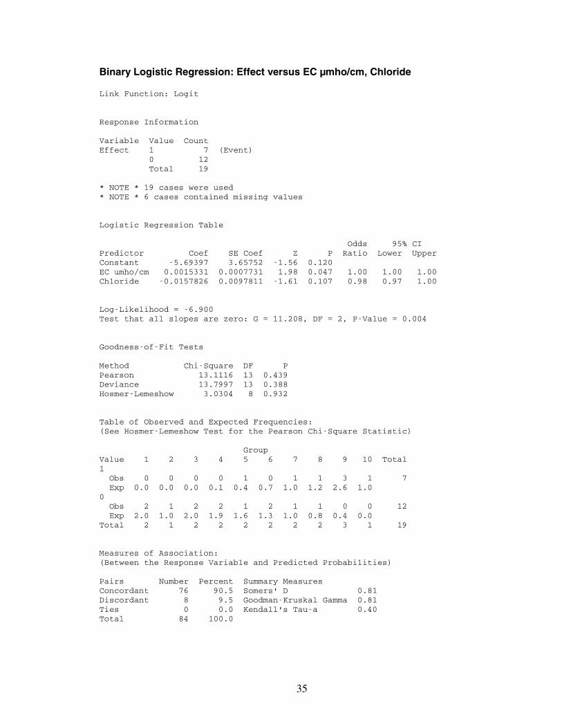
Binary Logistic Regression: Effect versus EC µmho/cm, Chloride

Link Function: Logit

Response Information

Variable Value CountEffect 1 7 (Event)

0 12Total 19

* NOTE * 19 cases were used* NOTE * 6 cases contained missing values

Logistic Regression Table

Odds 95% CIPredictor Coef SE Coef Z P Ratio Lower UpperConstant -5.69397 3.65752 -1.56 0.120EC umho/cm 0.0015331 0.0007731 1.98 0.047 1.00 1.00 1.00Chloride -0.0157826 0.0097811 -1.61 0.107 0.98 0.97 1.00

Log-Likelihood = -6.900Test that all slopes are zero: G = 11.208, DF = 2, P-Value = 0.004

Goodness-of-Fit Tests

Method Chi-Square DF PPearson 13.1116 13 0.439Deviance 13.7997 13 0.388Hosmer-Lemeshow 3.0304 8 0.932

Table of Observed and Expected Frequencies:(See Hosmer-Lemeshow Test for the Pearson Chi-Square Statistic)

GroupValue 1 2 3 4 5 6 7 8 9 10 Total1

Obs 0 0 0 0 1 0 1 1 3 1 7Exp 0.0 0.0 0.0 0.1 0.4 0.7 1.0 1.2 2.6 1.0

0Obs 2 1 2 2 1 2 1 1 0 0 12Exp 2.0 1.0 2.0 1.9 1.6 1.3 1.0 0.8 0.4 0.0

Total 2 1 2 2 2 2 2 2 3 1 19

Measures of Association:(Between the Response Variable and Predicted Probabilities)

Pairs Number Percent Summary MeasuresConcordant 76 90.5 Somers' D 0.81Discordant 8 9.5 Goodman-Kruskal Gamma 0.81Ties 0 0.0 Kendall's Tau-a 0.40Total 84 100.0

36


From the model based on an unbiased evaluation of the variables we can derive

the equation predicting stand loss based on NO3-N (lbs/acre) and Cu (mg/l) in the soil.

Since stand loss was considered complete or non-existent, complete stand loss is

represented by an effect value of 1 or greater value and non-existent stand loss is

represented by a 0 or less. The equation is as follows:

CuNEffect *523.7*532.370.12 ++−=

Where N is the lbs/acre of soil NO3-N and Cu is mg/l of copper in the soil before

application of swine effluent.

For the model based on biased evaluation of the variables we can derive the

equation predicting stand loss based on effluent values of EC (umho/cm) and Cl (mg/l).

The equation is as follows:

ClECEffect *0158.0*0015.06940.5 −++−=

Where EC is the electro conductivity in umho/cm for the effluent and Cl is mg/l

of chloride in the effluent.

The raw data and subsequent predictions of the two models are shown in Table

IV-d.

37

Farm

SoilNitrate

N(lbs/A)

SoilCu

(mg/l)

EffluentEC

(umho/cm)

EffluentChloride

(mg/l)

UnbiasedModel

CalculatedEffect

UnbiasedModel

TranslatedEffect

BiasedModel

CalculatedEffect

BiasedModel

TranslatedEffect

ObservedEffect

121 5 0.5 8970 562 -5.95 0 -1.12 0 0

121 2 1.6 8560 460 0.73 0.73 -0.12 0 0

40 10 0.9 5060 -0.28 0 1.90 1 0

40 10 0.9 5060 -0.28 0 1.90 1 1

40 19 7240 358 -2.27 0 -0.49 0 1

337 5 0.5 8290 511 -5.95 0 -1.33 0 0

278 2 0.6 11330 1164 -6.79 0 -7.09 0 0

278 12 0.6 11330 1164 -1.48 0 -7.09 0 0

299 7 5360 362 -8.65 0 -3.37 0 0

299 10 5360 362 -7.05 0 -3.37 0 0

301 5 8770 -9.71 0 7.46 1 0

299 5 10790 -9.71 0 10.49 1 0

301 14 0.9 11020 604 1.85 1 1.29 1 1

299 10 1.4 11200 605 3.48 1 1.55 1 1

299 22 1 11200 605 6.85 1 1.55 1 1

299 5 10790 -9.71 0 10.49 1 1

217 5 0.4 6870 277 -6.70 0 0.23 0.23 0

217 24 1 8200 221 7.92 1 3.11 1 1

43 10 1.2 6450 244 1.98 1 0.13 0.13 1

42 5 1 2150 186 -2.19 0 -5.41 0 0

42 12 4110 -5.99 0 0.47 0.47 0

42 17 0.12 6200 577 -2.43 0 -5.51 0 0

122 5 1 8100 443 -2.19 0 -0.54 0 0

122 5 1 6490 484 -2.19 0 -3.61 0 0

122 2 1.3 7430 476 -1.53 0 -2.07 0 1

Table IV-d. Comparison of models developed from the two sets of variables.

Conclusions

The unbiased model suggests that both the soil NO3-N (lbs/acre) and Cu (mg/l) in

soil had negative impacts on plant growth. Generally elevated levels of soil NO3-N only

have a positive effect on plant growth; however, since no commercial fertilizer was used,

the level of NO3-N may actually be an indication of the amount of effluent that has been

applied. For the unbiased model the effect of copper is somewhat suspect since 7 of the

25 data sets did not include a copper value for the soil. Additionally, it is possible that

the significant effect of Cu and NO3-N is an artifact of examining 55 possible variables

38

for only 25 data sets. The limited number of data sets and the high number of potentially

significant variables could lead to incorrectly identifying a variable as significant when it

is in fact, only a coincidence.

Evaluation of the model based on carefully selected variables, or the biased

model, yielded effluent values of EC (umho/cm) and Cl (mg/l) as potentially significant

variables. However, as Table IV-d shows, the biased model was less accurate at

predicting a negative stand impact than the unbiased model.

References

Ayers, R.S. and D.W. Westcot. 1985. Water quality for agriculture. Fao Irrigation andDrainage Paper 29 (Rev. 1), Food and Agriculture Organization (FAO) of the UnitedNations. Rome, Italy.

Bell, J.R., D.M. Caudle. 1994, June. Range, Wildlife and Fisheries Management.Management of Old World Bluestems. Retrieved From:http://www.rw.ttu.edu/newsletter/mgmtnotes.htm

Harmoney K.R. and K.R. Hickman. 2004. Comparative Morphology of Caucasian OldWorld Bluestem (Bothriochloa bladhii) and Native Grasses. Agronomy Journal. Vol.96:1540-1544.


.

39

Chapter V

Related Experiments

Effluent Application at Farm


A healthy stand of World bluestem of the WW-Iron Master variety was chosen

within a mile of other stands allegedly impacted by swine effluent application. Two

weeks before swine effluent application, an evenly vegetated 95 by 80 foot rectangle

within the chosen stand of Old World bluestem was chosen and watered with several

inches of water to encourage plant growth. The 95 by 80 foot rectangle was then divided

into 5 by 10 foot plots. A five foot buffer zone separated all plots from each other as

shown in Figure V-a.

50% 12.50% 0% 100% 25%

12.50% 100% 50% 25% 0%

25% 0% 100% 50% 12.50%

25% 12.50% 100% 0% 50%

100% 50% 12.50% 25% 0%

50% 25% 0% 12.50% 100%

0% 50% 12.50% 100% 25%

100% 25% 0% 50% 12.50%

12.50% 100% 25% 0% 50%

Figure V-a. Plot layout design.

40

The initial Normalized Difference Vegetation Index (NDVI) value was found for

each plot using the GreenSeeker. This was accomplished by passing the sensor over the

middle of each of the plots at a height of three feet while walking at a constant rate. Each

plot was read in triplicate.The plots were divided into the three sub-treatments: morning,

afternoon and evening effluent applications. Each sub-treatment contained three rows

each containing five plots randomly marked for each of the five different effluent

concentration applications. The red plots received undiluted swine effluent, the green

plots received 1:1 dilution of swine effluent to water, the blue plots received 1:3 dilution

of swine effluent to water, the yellow plots received a 1:7 dilution of swine effluent to

water and the white blocks received pure water. All treatments received about 31 gallons

of liquid, equivalent to one inch application depth.

Effluent application was divided into three portions of the day. The morning

application started at about 7:00 a.m. and lasted until 10:00 a.m. The afternoon

application began at 12:00 p.m. and ended at 3:00 p.m. The evening application began at

5:00 p.m. and ended at 8:00 p.m. To improve the chance of salt burn, application was

performed during a hot day with high solar radiation.

To obtain an even application of the treatment solution a specially designed

sprinkling system was used. The sprinkling system consisted of a 5’X10’ frame

containing 4 quarter-circle sprinkler heads (Rain Bird, 8Q, www.rainbird.com) in each

corner and 2 half-circle heads (Rain Bird, 8H, www.rainbird.com) in the middle of the 10

foot lengths as shown in Figures V-b and V-c.

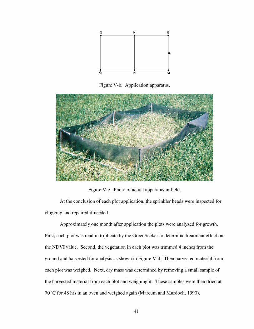
41

Figure V-b. Application apparatus.

Figure V-c. Photo of actual apparatus in field.

At the conclusion of each plot application, the sprinkler heads were inspected for

clogging and repaired if needed.

Approximately one month after application the plots were analyzed for growth.

First, each plot was read in triplicate by the GreenSeeker to determine treatment effect on

the NDVI value. Second, the vegetation in each plot was trimmed 4 inches from the

ground and harvested for analysis as shown in Figure V-d. Then harvested material from

each plot was weighed. Next, dry mass was determined by removing a small sample of

the harvested material from each plot and weighing it. These samples were then dried at

70o C for 48 hrs in an oven and weighed again (Marcum and Murdoch, 1990).

42

Figure V-d. Harvest of treated stands one month after application.

Reflectance Index Results

One month after application the stands were analyzed for treatment effects. One

method of determining the effect of swine effluent application was to compare the initial

and final reflectance index values measured by the Greenseeker. Although the detection

limit for the Greenseeker is 0.05, each treatment was recorded in triplicate to improve

testing resolution, the averages are shown in Table V-a. By measuring the difference

between initial and final reflectance index values we were able to quantify the effects of

the treatments. These results are summarized in Table V-b and Figure V-e.

43

Initial Final DifferenceOverall Overall

c Control 0.641 c Control 0.678 0.037e Eighth 0.640 e Eighth 0.660 0.020q Quarter 0.618 q Quarter 0.682 0.064h Half 0.645 h Half 0.670 0.026f Full 0.613 f Full 0.675 0.063

Average 0.631 Average 0.673 0.042

8 A.M. 8 A.M.c Control 0.626 c Control 0.622 -0.004e Eighth 0.632 e Eighth 0.675 0.043q Quarter 0.638 q Quarter 0.664 0.026h Half 0.632 h Half 0.665 0.032f Full 0.600 f Full 0.705 0.105


2 P.M. 2 P.M.c Control 0.654 c Control 0.686 0.032e Eighth 0.690 e Eighth 0.654 -0.036q Quarter 0.642 q Quarter 0.657 0.015h Half 0.678 h Half 0.677 -0.001f Full 0.657 f Full 0.666 0.010


8 P.M. 8 P.M.c Control 0.644 c Control 0.727 0.083e Eighth 0.597 e Eighth 0.651 0.054q Quarter 0.575 q Quarter 0.726 0.150h Half 0.624 h Half 0.669 0.046f Full 0.594 f Full 0.664 0.070


Table V-a. The average initial and final reflectance index for each treatment and theirdifference.

Overall 8 P.M. 2 P.M. 8 A.M.c Control 0.037 -0.004 0.032 0.083e Eighth 0.020 0.043 -0.036 0.054q Quarter 0.064 0.026 0.015 0.150h Half 0.026 0.032 -0.001 0.046f Full 0.063 0.105 0.010 0.070

Average 0.042 0.040 0.004 0.081

Table V-b. The average difference in reflectance index for each treatment afterapplication.

44

Average Change in Reflectance Index After Application

-0.050

0.000

0.050

0.100

0.150

0.200

Overall 8 P.M. 2 P.M. 8 A.M.

Treatment

Ch

ang

ein

Rel

fect

ance

Ind

ex

Control

Eighth

Quarter

Half

Full

Average

Figure V-e. The average difference in reflectance index for each treatment after

application.

Statistical analysis of the reflectance index results began with a two-way ANOVA

test to determine the effect of the time of application, the dilution of effluent, and their

interaction. As the following analysis shows, both the treatment and interaction terms

were insignificant at a 10% alpha value.

Two-way ANOVA: Change in Reflectance Index versus Time, Treatment

Source DF SS MS F PTime 2 0.031923 0.0159614 2.72 0.082Treatment 4 0.008942 0.0022355 0.38 0.820Interaction 8 0.035440 0.0044301 0.76 0.643Error 30 0.175751 0.0058584Total 44 0.252056

S = 0.07654 R-Sq = 30.27% R-Sq(adj) = 0.00%

Analysis of the two-way ANOVA also indicated that a one-way ANOVA with a

Tukey comparison of the change in the reflectance index versus time was also necessary.

45

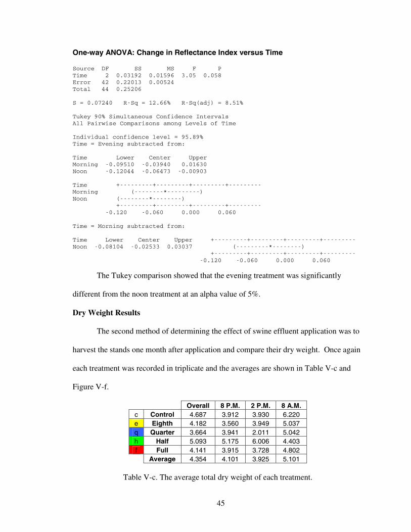
One-way ANOVA: Change in Reflectance Index versus Time

Source DF SS MS F PTime 2 0.03192 0.01596 3.05 0.058Error 42 0.22013 0.00524Total 44 0.25206

S = 0.07240 R-Sq = 12.66% R-Sq(adj) = 8.51%

Tukey 90% Simultaneous Confidence IntervalsAll Pairwise Comparisons among Levels of Time

Individual confidence level = 95.89%Time = Evening subtracted from:

Time Lower Center UpperMorning -0.09510 -0.03940 0.01630Noon -0.12044 -0.06473 -0.00903

Time +---------+---------+---------+---------Morning (--------*---------)Noon (--------*--------)

+---------+---------+---------+----------0.120 -0.060 0.000 0.060

Time = Morning subtracted from:

Time Lower Center Upper +---------+---------+---------+---------Noon -0.08104 -0.02533 0.03037 (---------*--------)

+---------+---------+---------+----------0.120 -0.060 0.000 0.060

The Tukey comparison showed that the evening treatment was significantly

different from the noon treatment at an alpha value of 5%.

Dry Weight Results

The second method of determining the effect of swine effluent application was to

harvest the stands one month after application and compare their dry weight. Once again

each treatment was recorded in triplicate and the averages are shown in Table V-c and

Figure V-f.

Overall 8 P.M. 2 P.M. 8 A.M.c Control 4.687 3.912 3.930 6.220e Eighth 4.182 3.560 3.949 5.037q Quarter 3.664 3.941 2.011 5.042h Half 5.093 5.175 6.006 4.403f Full 4.141 3.915 3.728 4.802

Average 4.354 4.101 3.925 5.101

Table V-c. The average total dry weight of each treatment.

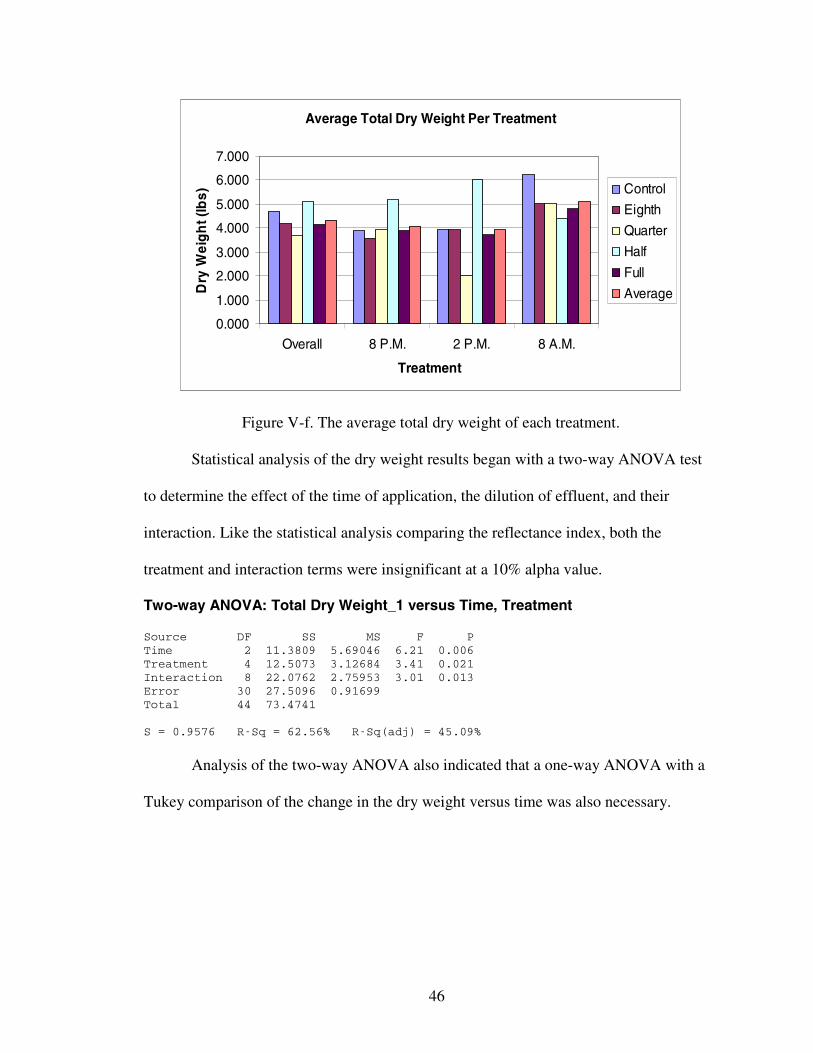
46

Average Total Dry Weight Per Treatment

0.000

1.000

2.000

3.000

4.000

5.000

6.000

7.000

Overall 8 P.M. 2 P.M. 8 A.M.

Treatment

Dry

Wei

gh

t(lb

s) Control

Eighth

Quarter

Half

Full

Average

Figure V-f. The average total dry weight of each treatment.

Statistical analysis of the dry weight results began with a two-way ANOVA test

to determine the effect of the time of application, the dilution of effluent, and their

interaction. Like the statistical analysis comparing the reflectance index, both the

treatment and interaction terms were insignificant at a 10% alpha value.

Two-way ANOVA: Total Dry Weight_1 versus Time, Treatment

Source DF SS MS F PTime 2 11.3809 5.69046 6.21 0.006Treatment 4 12.5073 3.12684 3.41 0.021Interaction 8 22.0762 2.75953 3.01 0.013Error 30 27.5096 0.91699Total 44 73.4741

S = 0.9576 R-Sq = 62.56% R-Sq(adj) = 45.09%

Analysis of the two-way ANOVA also indicated that a one-way ANOVA with a

Tukey comparison of the change in the dry weight versus time was also necessary.

47

One-way ANOVA: Total Dry Weight_1 versus Time

Source DF SS MS F PTime 2 11.38 5.69 3.85 0.029Error 42 62.09 1.48Total 44 73.47

S = 1.216 R-Sq = 15.49% R-Sq(adj) = 11.47%

Individual 95% CIs For Mean Based onPooled StDev

Level N Mean StDev ---+---------+---------+---------+------Evening 15 4.101 0.733 (--------*--------)Morning 15 5.069 1.306 (--------*--------)Noon 15 3.925 1.480 (--------*--------)

---+---------+---------+---------+------3.50 4.20 4.90 5.60

Pooled StDev = 1.216

Tukey 90% Simultaneous Confidence IntervalsAll Pairwise Comparisons among Levels of Time

Individual confidence level = 95.89%

Time = Evening subtracted from:

Time Lower Center Upper -------+---------+---------+---------+--Morning 0.032 0.968 1.904 (-------*-------)Noon -1.111 -0.176 0.760 (-------*------)

-------+---------+---------+---------+---1.2 0.0 1.2 2.4

Time = Morning subtracted from:

Time Lower Center Upper -------+---------+---------+---------+--Noon -2.079 -1.144 -0.208 (------*-------)

-------+---------+---------+---------+---1.2 0.0 1.2 2.4

The Tukey comparison showed that the morning treatment was significantly

different from both the noon and the evening treatments at an alpha value of 5% for the

change in the reflectance index data.

Conclusion

The experiment was designed to test the effect of various dilutions of swine

effluent applied at three different times of day on stand loss. Statistical analysis of both

the reflectance index and dry weight data indicated that the dilution had no significant

48

effect on stand growth. However, the statistical analysis of both the reflectance index and

dry weight data did indicate that the time of day of the application was significant at a

10% alpha level. A Tukey’s 90% confidence test showed that for the reflectance index

data the noon application was significantly different from the evening application. The

Tukey’s 90% confidence test for the dry weight data showed that the morning application

was significantly different from both the evening and noon applications. These results

are summarized in Table V-d and Figure V-g. While the reflectance index data and the

dry weight data do not agree on the magnitude of the differences between each group,

they do both indicate that an application of effluent at noon will result in the least positive

effect on plant growth. This may be a result of the higher evaporation effects at noon,

and subsequent decreased water available for plant growth.

Morning Noon EveningChange in Reflectance Index 0.0412 0.01587 0.0806

Average Total Dry Weight 5.069 3.925 4.101

Table V-d. Summary of the effects of the time of application.

Summary of the of Application Time Effect

0%20%40%60%80%

100%120%

Morning Noon Evening

Per

cen

tE

ffec

t

Change in Reflectance Index

Average Total Dry Weight

Figure V-g. Graphical comparison of application time effect. Percent effect is thepercent of the maximum observed effect of its type each represented.

49

Salt Solution Spray in Greenhouse

Materials and Methods

Six saline treatments from 1-20 ds/m were used to determine the extent of foliage

damage when saline solutions were applied to Old World bluestem. Each of the six

treatments included three 6-inch pots stored in a universal hydroponics solution tray.

Each pot contained three Old World bluestem plants of the WW-Iron Master variety

planted in five inches of silicon sand. Nutrients were supplied by Liquid Grow 7-9-5

(Dyna-Gro, www.dyna-gro.com) nutrient media mixed with water. During the first two

months plants were trimmed each week to a height of four inches to encourage root

development. Each week the hydroponics media was drained and replaced with fresh

media.

Once plants were established, the reflectance index for each pot was tested using

the Greenseeker. To obtain optimal Greenseeker readings, the Greenseeker was mounted

on a table while the pots were passed underneath. Care was taken to ensure the pots were

scanned by the Greenseeker at a nearly constant speed. Additionally, a defined track for

pot movement was created to ensure that the pots moved the same distance. Because the

detection limit of the Greenseeker is 0.05, each pot was scanned seven times and

averaged to minimize the variation.

The initial reflectance index values were used to order the pots by increasing

reflectance index. From this list the most uniform section of 18 pots was selected for the

study. To increase the uniformity of the treatments, the 18 pots were distributed amongst

the treatments so that the average of the initial reflectance index of each treatment was

nearly equal. The number for each pot and its corresponding treatment were recorded.

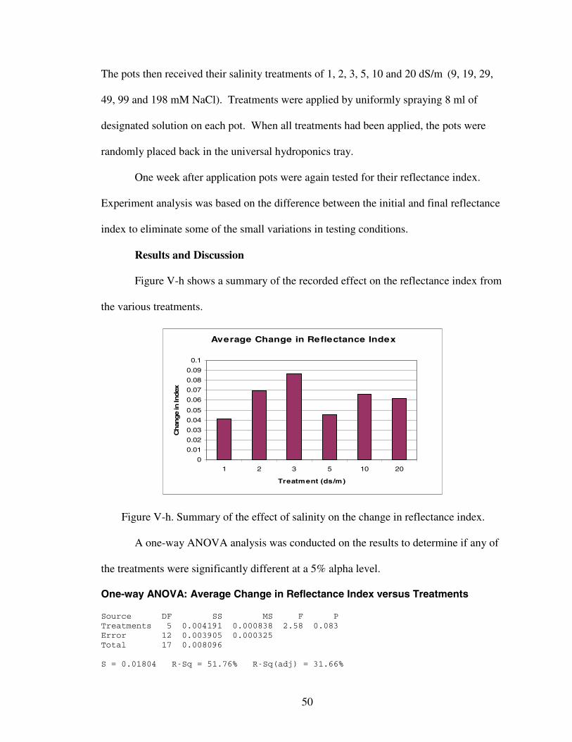
50

The pots then received their salinity treatments of 1, 2, 3, 5, 10 and 20 dS/m (9, 19, 29,

49, 99 and 198 mM NaCl). Treatments were applied by uniformly spraying 8 ml of

designated solution on each pot. When all treatments had been applied, the pots were

randomly placed back in the universal hydroponics tray.

One week after application pots were again tested for their reflectance index.

Experiment analysis was based on the difference between the initial and final reflectance

index to eliminate some of the small variations in testing conditions.


Figure V-h shows a summary of the recorded effect on the reflectance index from

the various treatments.

Average Change in Reflectance Index

0

0.01

0.02

0.03

0.04

0.05

0.06

0.07

0.08

0.09

0.1

1 2 3 5 10 20

Treatment (ds/m)

Chan

ge

inIn

dex

Figure V-h. Summary of the effect of salinity on the change in reflectance index.

A one-way ANOVA analysis was conducted on the results to determine if any of

the treatments were significantly different at a 5% alpha level.

One-way ANOVA: Average Change in Reflectance Index versus Treatments

Source DF SS MS F PTreatments 5 0.004191 0.000838 2.58 0.083Error 12 0.003905 0.000325Total 17 0.008096

S = 0.01804 R-Sq = 51.76% R-Sq(adj) = 31.66%

51

The ANOVA test did not yield a significant difference between treatments at a

5% alpha value for the reflectance index data.

Conclusion

At a 5% alpha level we conclude that none of the treatments had a significant

effect on the average change in the reflectance index. Additionally, since the average

reflectance index increased for all treatments, we may conclude that under these

conditions the plants did not suffer a significant salt burn effect. This may be because the

greenhouse environment was not an accurate representation of the conditions at the CRP

land, or because the application method was flawed.

Spray in Greenhouse with Quick Dry

Materials and Methods

The materials and methods for this experiment were the same as the previous

experiment with the exception of the treatments and the drying method used. For

controls, one treatment received no application while another received water at about

1ds/m. To test the potential for a salt burn from a pure salt solution, a solution of salt was

prepared at 100 ds/m (1000 mM NaCl). Additionally, 100%, 50% and 25% solutions of

swine effluent were also prepared for application. The swine effluent used was taken

from the waste stream of a shallow pit from a farrrowing barn. Treatments were applied

by uniformly spraying 16 ml of designated solution to each pot. Immediately following

application the plants were blown with 40o C air until all droplets on foliage had dried.

Heated air was provided by a hair dryer maintained 3 feet from the plants to imitate wind

during a hot day common to the CRP land. When all treatments had been applied, the

pots are randomly placed back in the universal hydroponics tray.

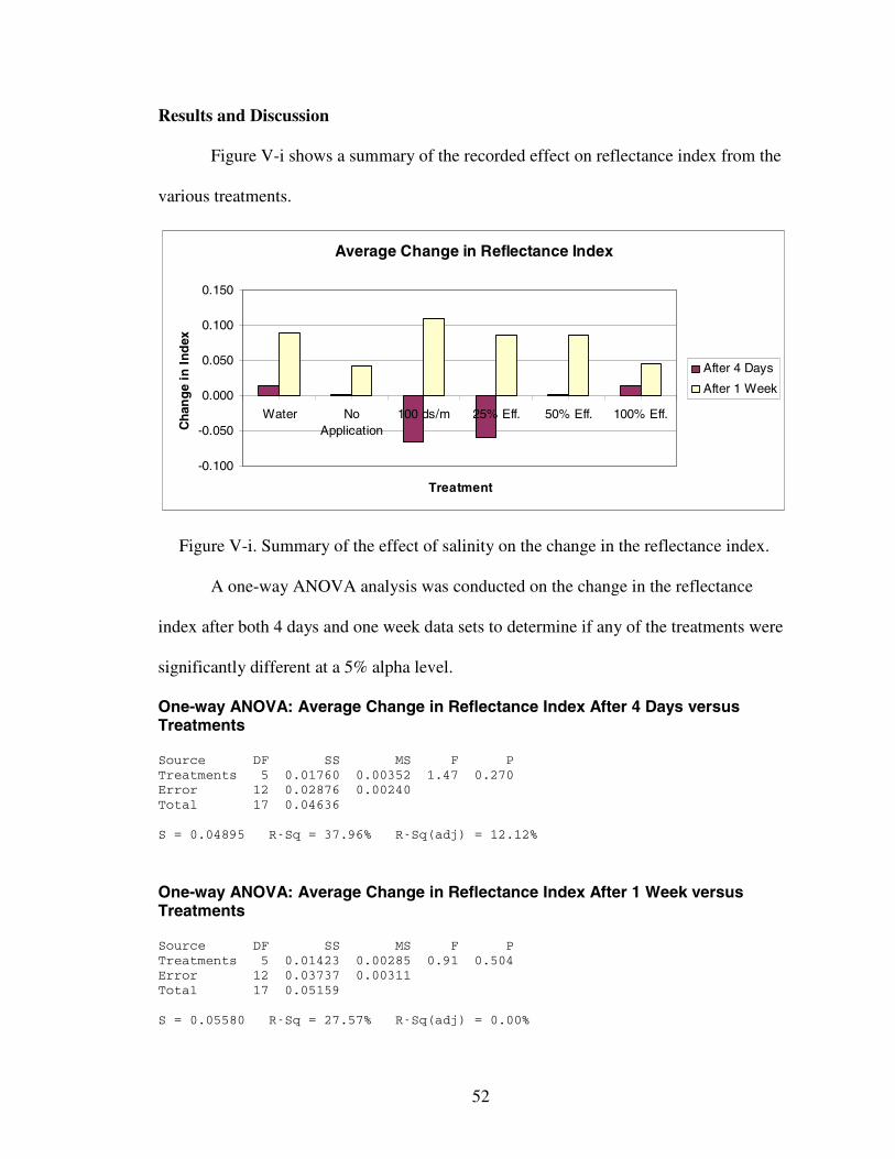
52


Figure V-i shows a summary of the recorded effect on reflectance index from the

various treatments.

Average Change in Reflectance Index

-0.100

-0.050

0.000

0.050

0.100

0.150

Water NoApplication

100 ds/m 25% Eff. 50% Eff. 100% Eff.

Treatment

Ch

ang

ein

Ind

ex

After 4 Days

After 1 Week

Figure V-i. Summary of the effect of salinity on the change in the reflectance index.

A one-way ANOVA analysis was conducted on the change in the reflectance

index after both 4 days and one week data sets to determine if any of the treatments were

significantly different at a 5% alpha level.

One-way ANOVA: Average Change in Reflectance Index After 4 Days versusTreatments


S = 0.04895 R-Sq = 37.96% R-Sq(adj) = 12.12%

One-way ANOVA: Average Change in Reflectance Index After 1 Week versusTreatments


S = 0.05580 R-Sq = 27.57% R-Sq(adj) = 0.00%

53

Neither of the ANOVA tests yielded a significant difference between the

treatments from the reflectance index data.

Conclusion

At a 5% alpha level we conclude that none of the treatments produced a

significant average change in the reflectance index for either the 4 day or 1 week data

sets. Additionally, since the average reflectance index after one week increased for all

treatments, we may conclude that under these conditions the plants did not suffer a

significant salt burn effect. It is interesting that plants sprayed with 100 ds/m solution

and a 25% effluent dilution did show a reflectance index reduction after 4 days, but

seemed to recover by the end of the week. It is possible that no effect was found from the

salt solution and swine effluent because the greenhouse environment was not an accurate

representation of the conditions at the CRP land, or because the application method was

flawed.

54

Chapter VI

Conclusions

The objectives and conclusions of this study were:

1. Determine the salinity tolerance threshold for WW-Iron Master Old World

bluestem;

The salt tolerance study indicated that WW-Iron Master Old World bluestem is a

highly salt sensitive plant. The salinity threshold for WW-Iron Master Old World

bluestem was found using the piecewise linear response model to be 1 ds/m. A

mineral analysis of the root and shoot portions of the studied plants indicated an

interaction between K+ and Na+ concentrations in the root tissue of WW-Iron Master

Old World bluestem. Additionally, the Na+ accumulation in the shoots was much

greater than in the roots, indicating that WW-Iron Master Old World bluestem is

unable to restrict Na+ transport.

2. Determine the fractional yield decline per unit increase in salinity beyond the

threshold;

The fractional yield decline per unit increase in salinity beyond the threshold for

WW-Iron Master Old World bluestem was found using the piecewise linear response

model to be 21%.

3. Determine if the time of day the effluent is applied to the plant has a significant

effect on plant growth;

55

From the statistical analysis of the results from the field study of swine effluent

application, both the reflectance index and dry weight data did indicate that the time

ofday of the application was significant at a 10% alpha level. A Tukey’s 90% confidence

test showed that for the reflectance index data the noon application was significantly

different from the evening application. The tukey’s 90% confidence test for the dry

weight data showed that the morning application was significantly different from both the

evening and noon applications. While reflectance index data and the dry weight data do

not agree on the magnitude of the differences between each group, they do both indicate

that an application of effluent at noon will result in the least positive effect on plant

growth. This may be a result of the higher evaporation effects at midday, and subsequent

decreased water available for plant growth.

4. Determine the optimum dilutions for swine effluent when applied to WW-Iron

Master Old World bluestem;

From the field study of swine effluent application, no effect on plant growth was

statistically significant due to the effluent dilutions.

5. Verify that using the “Greenseeker” is an adequate method for determining

salinity effects on plant growth;

The “Greenseeker” was shown capable of quantifying plant growth in a non-

invasive manner. However, because salt burn studies were unable to produce a

negative impact on plant tissue, the experiments could not test the suitability of the

“Greenseeker” for determining salt burn effects on plant growth.

6. Determine if a salt solution spray on foliage can cause plant damage;

56

Greenhouse studies investigating salt burn never produced a statistically

significant effect of salt or swine effluent dilutions on WW-Iron Master Old World

bluestem. Since the average reflectance index after one week increased for all

treatments, with and without quick drying conditions, we may conclude that under these

conditions the plants did not suffer a significant salt burn effect.

7. Determine if foliage burn during swine effluent application is a result of chemical

constituents other than salts;

Neither the salt solutions nor the swine effluent solutions caused a burn effect on

the plant tissue. Consequently, no evidence was provided that non-salt constituents of

swine effluent could cause salt burns on WW-Iron Master Old World bluestems.

8. Statistically evaluate application data from the Conservation Reserve Program.

The unbiased model suggests that both the soil NO3-N (lbs/acre) and Cu (mg/l) in

soil had negative impacts on plant growth. However, the limited number of data sets and

the high number of potentially significant variables could lead to incorrectly identifying a

variable as significant when it is in fact only a coincidence. Evaluation of the model

based on carefully selected variables, or the biased model, yielded effluent values of EC

(umho/cm) and Cl (mg/l) as potentially significant variables. However, the biased model

was less accurate at predicting a negative stand impact than the unbiased model.

Recommendations for Future Studies

Although the studies completed in this thesis show that Old World bluestem is a

highly salt-sensitive plant, further investigation is needed to determine under what

conditions, if any, application of effluent will result in salt burn on the leaves. Studies of

57

salt burn effects in this thesis were never able to replicate the reported effects on CRP

land. Further studies should consider the possibility for sequential wetting and drying

cycles during a single application of effluent. This would require application during hot

windy days with an application apparatus that does not provide continuous wetting. A

slow moving big gun assembly may be the missing element in the salt burn studies

conducted in this thesis.

The statistical approach to the data gathered from the CRP land requires more

replications to provide reliable interpretation. Additionally, statistical analysis would

improve with a more complete data set that required fewer assumptions. It is

recommended that further research includes an on-site observation of soil and effluent

sample collection and land application methods.

58

References

Bell, J.R., D.M. Caudle. 1994, June. Range, Wildlife and Fisheries Management.Management of Old World Bluestems. Retrieved From:http://www.rw.ttu.edu/newsletter/mgmtnotes.htm

Cheeseman, J. M. 1988. Mechanisms of salinity tolerance in plants. Plant Physiol. 87,547–550.

Cummings, B. Pearson Education Inc. (n.d.). Retrieved December 1, 2006, fromhttp://www.soils.wisc.edu/courses/soils326/root%20xsection.gif

Harmoney K.R. and K.R. Hickman. 2004. Comparative Morphology of Caucasian OldWorld Bluestem (Bothriochloa bladhii) and Native Grasses. Agronomy Journal. Vol.96:1540-1544.

Hoffman, G.J., R.S. Ayers, E.J. Doering and B.L. McNeal. 1980. Salinity in IrrigatedAgriculture. In: Design and Operation of Farm Irrigation Systems. M.E. Jensen, Editor.ASAE Monograph No. 3. St. Joseph, MI. 829pp.

Hydroponics As A Hobby Retrieved September 6, 2006, fromhttp://plantanswers.tamu.edu/publications/hydroponics.html

Jones, J. B. 1997. Hydroponics, a practical guide for the soilless grower. St. Lucie Press,Boca Raton, FL 33431. 230 pp.

Kelling, K.A., and M.A. Schmitt. 2003. Applying manure to alfalfa: Pros, cons andrecommendations for three application strategies. N. Central Reg. Res. Rep. 346. CollegeAgric. Life Sci., Univ. of Wisconsin, Madison.

Marcum, K.B. and Murdoch, C.L. 1990. Growth responses, ion relations, and osmoticadaptations of eleven C4 Turfgrasses to salinity. Agronomy Journal 82: 892–896.

O'Leary, J. W. 1969. The effect of salinity on permeability of roots to water. Isr. J. Bot.18, 1–9

Passioura, J.B. 1988. Water transport in and to roots. Annu Rev Plant Physiol Plant MolBiol. 39: 245–265.

59


Steudle, E. 1994. Water transport across roots. Plant and Soil Volume 167, Number 1 /November, 1994

60

Appendices

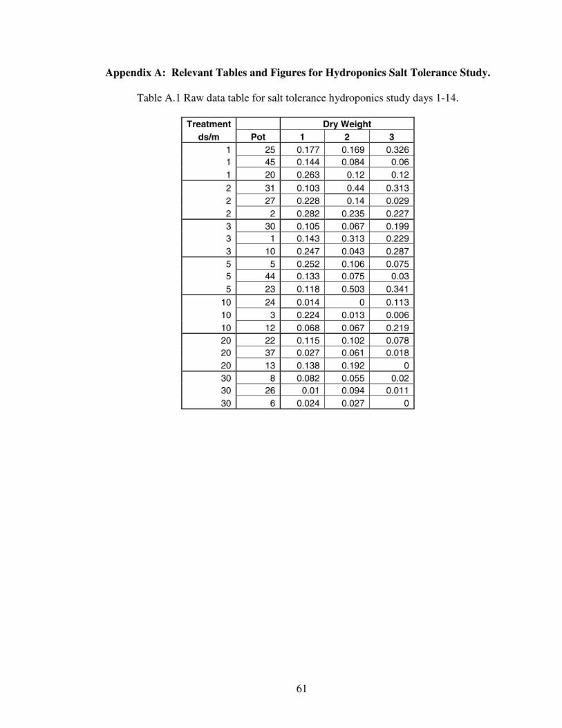
61

Appendix A: Relevant Tables and Figures for Hydroponics Salt Tolerance Study.

Table A.1 Raw data table for salt tolerance hydroponics study days 1-14.

Treatment Dry Weightds/m Pot 1 2 3

1 25 0.177 0.169 0.3261 45 0.144 0.084 0.061 20 0.263 0.12 0.12

2 31 0.103 0.44 0.3132 27 0.228 0.14 0.0292 2 0.282 0.235 0.2273 30 0.105 0.067 0.1993 1 0.143 0.313 0.2293 10 0.247 0.043 0.2875 5 0.252 0.106 0.0755 44 0.133 0.075 0.035 23 0.118 0.503 0.341

10 24 0.014 0 0.11310 3 0.224 0.013 0.00610 12 0.068 0.067 0.21920 22 0.115 0.102 0.07820 37 0.027 0.061 0.01820 13 0.138 0.192 030 8 0.082 0.055 0.0230 26 0.01 0.094 0.01130 6 0.024 0.027 0

62



1 25 0.15 0.094 0.2551 45 0.119 0.098 0.1171 20 0.065 0.11 0.193

2 31 0.031 0.112 0.0962 27 0.175 0.111 0.122 2 0.255 0.589 0.253 30 0.092 0.026 0.0473 1 0.104 0.49 0.1293 10 0.049 0.032 0.2695 5 0.288 0.01 0.0355 44 0.038 0.032 0.0485 23 0.025 0.046 0.31

10 24 0.094 0.057 0.00210 3 0 0.015 0.11510 12 0.078 0.234 0.14620 22 0.054 0 0.02420 37 0.004 0.021 020 13 0.053 0.014 030 8 0.024 0 030 26 0 0 030 6 0 0 0.01

63



1 25 0.153 0.185 0.1661 45 0.154 0.109 0.1491 20 0.069 0.098 0.201

2 31 0.023 0.282 0.1322 27 0.128 0.133 0.1722 2 0.098 0.137 0.2813 30 0.047 0.063 0.0893 1 0.049 0.241 0.0623 10 0.032 0.011 0.0865 5 0.008 0.017 0.0275 44 0.061 0.005 0.055 23 0.016 0.117 0.179

10 24 0.029 0 010 3 0.014 0.021 0.05710 12 0.002 0.088 0.10320 22 0 0 020 37 0 0 020 13 0 0 030 8 0 0 030 26 0 0 030 6 0 0 0

64



1 25 0.187 0.176 0.2581 45 0.25 0.238 0.3071 20 0.127 0.239 0.268

2 31 0.028 0.134 0.1162 27 0.161 0.185 0.1352 2 0.107 0.163 0.2113 30 0.023 0.043 0.0683 1 0.06 0.284 0.0843 10 0.076 0.039 0.095 5 0.041 0.015 0.0135 44 0.049 0.023 0.0265 23 0.014 0.133 0.177

10 24 0.031 0 010 3 0.028 0.013 0.0310 12 0.006 0.072 0.0720 22 0 0 020 37 0 0 020 13 0 0 030 8 0 0 030 26 0 0 030 6 0 0 0

65

Table A.5 Raw nutrient concentration data table showing mineral content from bi-weeklycuttings for salt tolerance hydroponics study. When plant growth was insufficient for

nutrient analysis an “x” was used to represent the missing data points.

Period ds/m %P %Ca %K %Mg %Na %SppmFe

ppmZn

ppmCu

ppmMn

Days 1-14 1 0.42 0.19 2.12 0.12 0.03 0.11 119.36 26.52 28.03 69.022 0.51 0.16 2.24 0.11 0.09 0.10 84.67 60.69 89.33 95.303 0.30 0.09 1.27 0.07 0.06 0.06 32.24 13.61 12.28 63.545 0.26 0.07 1.37 0.07 0.12 0.06 42.07 20.00 26.35 49.3710 0.50 0.14 2.25 0.11 0.52 0.10 77.21 43.14 80.86 134.8320 0.42 0.16 2.20 0.11 1.49 0.12 87.01 26.34 33.88 144.7230 0.39 0.13 2.19 0.11 2.68 0.14 72.44 168.86 274.87 148.10

Days 14-28 1 0.44 0.20 2.39 0.11 0.03 0.09 56.77 37.76 46.62 55.552 0.50 0.17 2.34 0.10 0.07 0.09 58.94 25.23 33.23 104.983 0.46 0.15 2.28 0.12 0.11 0.08 58.66 29.40 25.40 104.905 0.46 0.12 2.44 0.10 0.59 0.10 67.73 29.46 29.31 97.5610 x x x x x x x x x x20 x x x x x x x x x x30 x x x x x x x x x x

Days 28-42 1 0.53 0.22 3.03 0.12 0.03 0.09 57.77 27.60 27.75 40.992 0.52 0.18 2.38 0.11 0.09 0.08 56.63 18.34 17.56 101.073 0.64 0.24 2.63 0.15 0.23 0.10 53.97 62.35 88.77 140.715 0.56 0.22 3.10 0.14 0.77 0.15 112.74 26.86 31.24 130.8310 0.50 0.17 2.50 0.14 0.70 0.15 359.74 50.73 217.80 255.8420 x x x x x x x x x x30 x x x x x x x x x x

Days 42-56 1 0.58 0.22 3.37 0.12 0.03 0.09 49.76 23.45 21.57 34.772 0.66 0.21 3.00 0.12 0.18 0.10 71.69 29.44 38.17 90.993 0.73 0.21 3.09 0.15 0.34 0.10 58.41 20.48 18.15 118.055 0.59 0.16 2.87 0.11 1.19 0.14 55.47 82.32 127.78 116.3410 x x x x x x x x x x20 x x x x x x x x x x30 x x x x x x x x x x

66

Table A.6 Raw nutrient concentration data table showing final mineral content for thebottom 4” of foliage and the root tissue used in the salt tolerance hydroponics study.

Foliage content above 4” is shown in earlier data table.

ds/m Sample %P %Ca %K %Mg %Na %S ppm Fe ppm Zn ppm Cu ppm Mn1 Below 4" 0.51 0.25 2.06 0.13 0.36 0.05 182.69 48.48 64.60 177.741 Root Zone 0.86 0.44 1.65 0.15 0.49 0.10 1947.65 94.32 277.97 391.622 Below 4" 0.70 0.41 1.26 0.14 0.81 0.07 773.61 89.09 284.87 194.022 Root Zone 0.78 0.29 1.48 0.12 0.50 0.10 1590.21 83.25 276.14 509.963 Below 4" 0.49 0.12 1.05 0.08 0.70 0.05 268.36 36.96 65.21 164.593 Root Zone 0.57 0.36 1.17 0.12 0.53 0.11 1840.97 59.75 196.32 448.745 Below 4" 0.50 0.21 1.08 0.10 1.43 0.07 373.30 55.88 112.33 238.005 Root Zone 0.61 0.36 0.98 0.10 0.80 0.10 1843.22 48.15 190.98 303.44

10 Below 4" 0.63 0.15 1.21 0.12 2.46 0.12 367.50 58.39 151.12 269.7010 Root Zone 0.87 0.28 1.11 0.11 1.44 0.11 1445.67 58.66 155.00 468.7420 Below 4" 0.59 0.37 1.20 0.12 6.95 0.11 1021.46 55.32 202.44 221.1820 Root Zone 0.77 0.29 0.55 0.10 1.94 0.16 1595.94 46.94 177.80 239.2130 Below 4" 0.43 0.25 1.23 0.13 9.24 0.11 414.53 61.45 200.09 175.9930 Root Zone 0.43 0.23 0.25 0.08 2.50 0.14 1493.68 38.27 155.26 165.01

Figure A.1 Comparison of basic mineral composition of roots from plants grown invarious salt concentrations for salt tolerance hydroponics study.

Basic Mineral Composition in Roots

0

0.5

1

1.5

2

2.5

3

1 2 3 5 10 20 30

ds/m of Sample

%C

om

po

siti

on %P

%Ca

%K

%Mg

%Na

%S

67

Figure A.2 Comparison of comparing trace mineral composition of roots from plantsgrown in various salt concentrations for salt tolerance hydroponics study.

Trace Mineral Composition in Roots

0

100

200

300

400

500

600

1 2 3 5 10 20 30

ds/m of Sample

pp

m

ppm Zn

ppm Cu

ppm Mn

Figure A.3 Comparison of basic mineral composition of bottom 4” of shoots from plantsgrown in various salt concentrations for salt tolerance hydroponics study.

Basic Mineral Composition in Bottom 4"

0

2

4

6

8

10

1 2 3 5 10 20 30

ds/m of Sample

%C

om

po

siti

on %P

%Ca

%K

%Mg

%Na

%S

68

Figure A.4 Comparison of trace mineral composition of bottom 4” of shoots from plantsgrown in various salt concentrations for salt tolerance hydroponics study.

Trace Mineral Composition in Bottom 4"

0

50

100

150

200

250

300

1 2 3 5 10 20 30

ds/m of Sample

pp

m

ppm Zn

ppm Cu

ppm Mn

69

Appendix B: Relevant Tables and Figures for Statistical Study of Swine EffluentApplication on Old World Bluestem.

Table B.1 Variables used to link application dates with specific fields.

Field Identification DataID # Farm Name # Application Date Coordinates Field Effect

1 121 Morris 418 4/1/2004 09-04-12 SE 02 121 Morris 418 7/21/2005 09-04-12 SE 03 40 Long 4917 6/28/1999 27-04-11 SW 14 40 Long 4917 5/24/1999 27-04-11 NW 15 40 Long 4917 4/19/2002 27-04-11 SW 16 337 Roberts 4574 7/21/2003 07-05-17 SE 07 278 Beelman 4606 12/21/2003 09-01-17 SE 08 278 Beelman 4606 12/15/2003 09-01-17 NE 09 299 Reust 2748 7/26/1999 20-01-15 SW 110 299 Reust 2748 7/19/1999 20-01-15 WNE 111 301 Reust 2748 9/24/2001 20-01-15 NW 112 299 Reust 2748 8/30/2001 20-01-15 SW 113 301 Reust 2748 9/3/2003 20-01-15 NW 114 299 Reust 2748 8/25/2003 20-01-15 SW 115 299 Reust 2748 8/14/2003 20-01-15 WNE 116 299 Reust 2748 8/27/2001 20-01-15 NE 117 217 Mouser 4720 5/11/1999 15-06-16 SW 118 217 Mouser 4720 9/11/1999 15-06-16 SW 119 43 Cliff 5321 4615 8/22/1999 05-04-10 SW 120 42 Hixon 4600 7/12/1999 11-04-10 NE 021 42 Hixon 4600 9/7/2001 11-04-10 NE 022 42 Hixon 4600 11/14/2002 11-04-10 SE 023 122 Hill 1913 8/24/1999 34-02-14 NW 124 122 Hill 1913 4/29/2003 34-02-14 NW 125 122 Hill 1913 7/20/2005 34-02-14 NW 1

70

Table B.2 General application conditions.

General Application Conditions

ID #Acre

Inches/AcreMax

Temp.Min

Humidity

MaxWind

DuringRain

During

RainfallWithinWeekAfter

RainfallWithinWeekBefore Season Month

1 0.89 87 6 43 0.05 0.57 0 Spring 32 0.42 101 18 34.5 0 0.01 1.39 Summer 73 0.90 102 13 40.8 0.01 1.27 0.93 Summer 64 1.62 89 13 48.9 0.03 0.62 0 Spring 55 0.62 92 6 53.7 0.27 0.14 0 Spring 46 0.94 108 9 42.6 0.29 0 0 Summer 77 0.92 65 11 32.6 0 0.04 0.14 Winter 128 0.81 72 18 59.3 0.14 0.04 0 Winter 129 1.47 101 19 37.8 0.13 0 0.07 Summer 710 1.54 98 21 35.6 0.2 0 0 Summer 711 0.81 91 10 34.8 0.26 0 0 Fall 912 0.67 99 13 42.4 0.61 0 0.07 Summer 813 0.62 103 17 43.9 0.52 0.51 0 Summer 814 0.76 103 17 43.9 0 0.52 0.67 Summer 815 0.60 103 16 60 0.67 0 1.58 Summer 816 0.75 99 13 42.4 0.63 0 0.05 Summer 817 1.12 84 15 48.9 2.26 0 0.59 Spring 518 1.76 101 9 36 0.4 0.24 0 Fall 919 1.71 102 34 39.5 0.6 0.28 0.41 Summer 820 2.15 98 25 43.5 1.34 0.13 0 Summer 721 1.89 98 11 51.2 0 0.15 0.19 Summer 822 1.23 78 13 43.9 0.11 0 1.51 Fall 1123 2.11 102 11 39.5 0.06 0.28 0.41 Summer 824 0.66 86 11 67.3 0.49 0 0 Spring 425 0.78 101 19 37 0 0.01 1.39 Summer 7

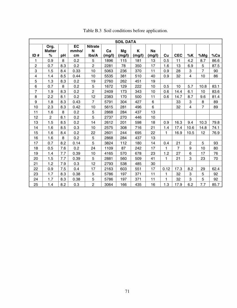
71

Table B.3 Soil conditions before application.

SOIL DATA

ID #

Org.Matter

% pH

ECmmho/

cm

NitrateN

lbs/ACa

(mg/l)Mg

(mg/l)K

(mg/l)Na

(mg/l) Cu CEC %K %Mg %Ca1 0.9 8 0.2 5 1896 115 181 13 0.5 11 4.2 8.7 86.62 0.7 8.3 0.2 2 2281 78 350 17 1.6 13 6.9 5 87.53 1.5 8.4 0.33 10 5063 236 370 11 0.9 28 3 7 904 1.4 8.5 0.44 10 5535 381 510 40 0.9 32 4 10 865 1.3 8.3 0.2 19 2760 262 451 196 0.7 8 0.2 5 1672 129 222 10 0.5 10 5.7 10.8 83.17 1.9 8.3 0.2 2 2409 173 343 10 0.6 14.4 6.1 10 83.68 2.2 8.1 0.2 12 2383 170 500 11 0.6 14.7 8.7 9.6 81.49 1.8 8.3 0.43 7 5791 304 427 6 33 3 8 8910 2.3 8.3 0.42 10 5615 281 496 6 32 4 7 8911 1.6 8 0.2 5 2868 284 437 1312 2 8.1 0.2 5 2737 270 446 1013 1.5 8.5 0.2 14 2612 201 598 18 0.9 16.3 9.4 10.3 79.814 1.6 8.5 0.3 10 2575 308 716 21 1.4 17.4 10.6 14.8 74.115 1.6 8.4 0.2 22 2601 244 695 22 1 16.9 10.5 12 76.916 1.6 8 0.2 5 2868 284 437 1317 0.7 8.2 0.14 5 3824 112 180 14 0.4 21 2 5 9318 0.5 7.6 0.2 24 1109 87 242 17 1 7 9 10 8019 1.4 7.7 0.39 10 4165 570 678 23 1.2 27 6 17 7620 1.5 7.7 0.39 5 2881 560 509 41 1 21 3 23 7021 1.2 7.9 0.3 12 2793 538 485 3022 0.9 7.5 0.4 17 2163 603 551 17 0.12 17.3 8.2 29 62.423 1.7 8.3 0.38 5 5786 197 371 11 1 32 3 5 9224 1.7 8.3 0.38 5 5786 197 371 11 1 32 3 5 9225 1.4 8.2 0.3 2 3064 166 435 16 1.3 17.9 6.2 7.7 85.7

72

Table B.4 Application effluent properties Part 1

Application Effluent Data Part 1

ID#

ECumho/cm pH

OrgN

(mg/l)Ammoniacal

NTot P(mg/l)

TotalSolids(mg/l) TVS TDS TSS

TotCa

(mg/l)1 8970 8.13 116 517 40.4 5685 1895 5275 410 97.72 8560 7.91 157 553 59.7 5315 2630 4270 1045 1413 5060 8.4 40 35 2000 1000 3238 1000 904 5060 8.4 40 35 2000 1000 3238 1000 905 7240 7.74 227 673 41.3 3640 1880 4706 220 82.56 8290 8.06 50 581 57.5 4240 1410 4040 200 77.77 11330 8.21 141 259 85.9 10305 3295 8142 2163 1258 11330 8.21 141 259 85.9 10305 3295 8142 2163 1259 5360 8 110 830 57 5000 2000 3430 3000 12010 5360 8 110 830 57 5000 2000 3430 3000 12011 8770 8.26 144 34.3 6624 5613 255 7612 10790 8.09 774 30.1 5476 1732 495 92.913 11020 8.11 141 832 53.4 6065 1870 5843 222 65.214 11200 8.18 103 761 61.2 7190 2465 6957 233 54.115 11200 8.18 103 761 61.2 7190 2465 6957 233 54.116 10790 8.09 774 30.1 5476 1732 495 92.917 6870 8.7 120 780 44 3000 1000 4397 8018 8200 7.9 90 770 53 3000 1000 5248 8019 6450 8.4 70 630 61 3000 1000 4128 8020 2150 8.7 10 26 2000 0 2150 7021 4110 8.17 15 53.5 2800 2630 340 12322 6200 8.2 105 271 44.4 4635 1975 4030 208 48.123 8100 7.4 30 540 44 5000 2000 5171 11024 6490 8.3 140 476 37.1 5680 2315 5370 310 89.725 7430 8.12 125 340 41.7 5125 1920 4.617 508 104

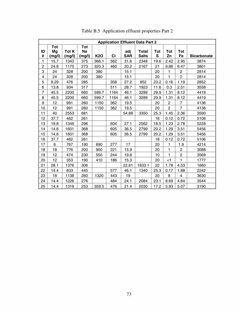
73

Table B.5 Application effluent properties Part 2

Application Effluent Data Part 2

ID#

TotMg

(mg/l)Tot K(mg/l)

TotNa

(mg/l) K2O Cladj

SARTotalSalts

TotS

TotZn

TotFe Bicarbonate

1 15.7 1343 375 366.1 562 31.6 2348 19.6 2.42 2.95 38742 24.8 1175 273 320.3 460 20.2 2167 21 9.88 6.47 38013 24 328 200 380 15.1 20 1 2 28144 24 328 200 380 15.1 20 1 2 28145 8.29 476 285 358 27.2 852 23.2 0.16 1.19 28526 13.8 934 317 511 28.7 1923 11.6 0.3 2.51 35587 45.5 2200 660 599.7 1164 46.1 3289 29.9 1.31 8.12 44198 45.5 2200 660 599.7 1164 46.1 3289 29.9 1.31 8.12 44199 12 991 260 1150 362 19.5 20 2 7 413610 12 991 260 1150 362 19.5 20 2 7 413611 40 2553 681 54.88 3350 25.3 1.45 2.36 359012 37.7 462 261 18 0.12 0.72 510613 19.8 1349 296 604 27.1 2562 18.5 1.23 2.78 522814 14.6 1601 368 605 36.5 2799 20.2 1.29 3.51 545615 14.6 1601 368 605 36.5 2799 20.2 1.29 3.51 545616 37.7 462 261 18 0.12 0.72 510617 6 767 190 890 277 17 20 1 1.9 421418 18 776 200 900 221 15.9 20 1 2 308819 12 474 230 550 244 19.8 10 1 2 356920 12 353 190 410 186 15.3 20 <1 1 177721 28.1 1376 306 22.61 1833.1 22 1.78 4.53 166022 14.4 833 445 577 46.1 1340 25.3 0.17 1.88 224223 18 1138 260 1320 443 19 20 8 4 363024 14.4 1226 276 484 24.1 2084 23.1 8.69 4.64 354425 14.4 1319 253 359.5 476 21.4 2030 17.2 5.93 5.07 3190

74

Appendix C: Relevant Tables and Figures for Related Experiments.

Figure C.1. Reflectance index from plots before swine effluent application for panhandlestudy.

0.599 0.562 0.589 0.56 0.522Block 18 P.M. 0.527 0.517 0.585 0.529 0.636

0.675 0.707 0.705 0.687 0.703

0.646 0.699 0.735 0.639 0.736Block 22 P.M. 0.673 0.7 0.745 0.739 0.762

0.598 0.541 0.562 0.627 0.562

0.584 0.72 0.763 0.715 0.724Block 38 A.M. 0.564 0.564 0.662 0.635 0.619

0.513 0.485 0.625 0.632 0.542

75

Figure C.2. Reflectance index from plots after swine effluent application for panhandlestudy. The red plots received undiluted swine effluent, the green plots received 1:1

dilution of swine effluent to water, the blue plots received 1:3 dilution of swine effluentto water, the yellow plots received a 1:7 dilution of swine effluent to water and the white

blocks received pure water

0.641 0.667 0.727 0.691 0.75Block 18 P.M. 0.643 0.619 0.663 0.688 0.738

0.739 0.717 0.681 0.704 0.644

0.649 0.669 0.629 0.688 0.691Block 22 P.M. 0.683 0.696 0.64 0.718 0.743

0.643 0.605 0.627 0.654 0.687

0.537 0.665 0.757 0.746 0.625Block 38 A.M. 0.68 0.679 0.639 0.666 0.626

0.641 0.663 0.688 0.69 0.663

Figure C.3. The final weight in lbs of harvested material from plots for panhandle study.

7.65 5.98 5.76 5.93 5.59Block 18 P.M. 4.53 5.14 7.25 6.67 7.48

5.29 5.83 6.49 6.32 6.44

4.87 6.49 5.67 6.15 10.04Block 2 3.57 11.832 P.M. 9.83 7.32 7.46

7.08 6.54 5.61 5.29 6.35

4.09 5.7 8.61 8.62 6.75Block 38 A.M. 6.34 7.3 10.08 5.95 6.76

6.74 5.48 6.28 7.1 6.92

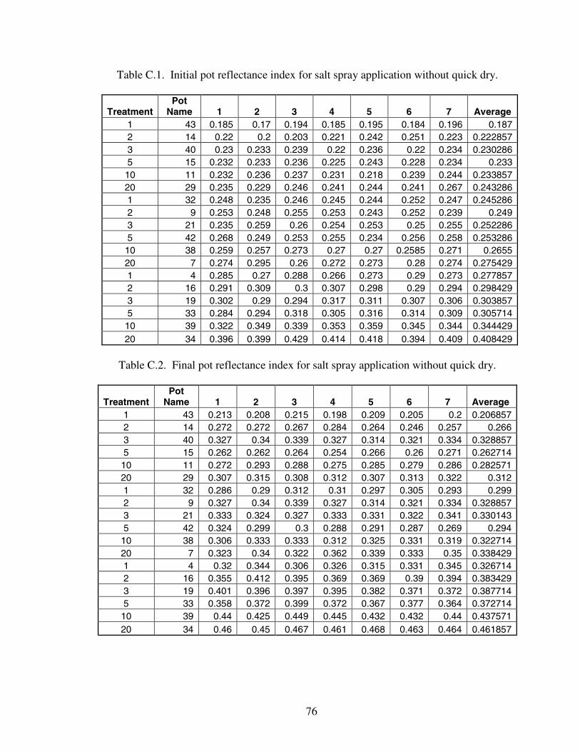
76

Table C.1. Initial pot reflectance index for salt spray application without quick dry.

TreatmentPot

Name 1 2 3 4 5 6 7 Average1 43 0.185 0.17 0.194 0.185 0.195 0.184 0.196 0.1872 14 0.22 0.2 0.203 0.221 0.242 0.251 0.223 0.2228573 40 0.23 0.233 0.239 0.22 0.236 0.22 0.234 0.2302865 15 0.232 0.233 0.236 0.225 0.243 0.228 0.234 0.23310 11 0.232 0.236 0.237 0.231 0.218 0.239 0.244 0.23385720 29 0.235 0.229 0.246 0.241 0.244 0.241 0.267 0.2432861 32 0.248 0.235 0.246 0.245 0.244 0.252 0.247 0.2452862 9 0.253 0.248 0.255 0.253 0.243 0.252 0.239 0.2493 21 0.235 0.259 0.26 0.254 0.253 0.25 0.255 0.2522865 42 0.268 0.249 0.253 0.255 0.234 0.256 0.258 0.25328610 38 0.259 0.257 0.273 0.27 0.27 0.2585 0.271 0.265520 7 0.274 0.295 0.26 0.272 0.273 0.28 0.274 0.2754291 4 0.285 0.27 0.288 0.266 0.273 0.29 0.273 0.2778572 16 0.291 0.309 0.3 0.307 0.298 0.29 0.294 0.2984293 19 0.302 0.29 0.294 0.317 0.311 0.307 0.306 0.3038575 33 0.284 0.294 0.318 0.305 0.316 0.314 0.309 0.30571410 39 0.322 0.349 0.339 0.353 0.359 0.345 0.344 0.34442920 34 0.396 0.399 0.429 0.414 0.418 0.394 0.409 0.408429

Table C.2. Final pot reflectance index for salt spray application without quick dry.

TreatmentPot

Name 1 2 3 4 5 6 7 Average1 43 0.213 0.208 0.215 0.198 0.209 0.205 0.2 0.2068572 14 0.272 0.272 0.267 0.284 0.264 0.246 0.257 0.2663 40 0.327 0.34 0.339 0.327 0.314 0.321 0.334 0.3288575 15 0.262 0.262 0.264 0.254 0.266 0.26 0.271 0.26271410 11 0.272 0.293 0.288 0.275 0.285 0.279 0.286 0.28257120 29 0.307 0.315 0.308 0.312 0.307 0.313 0.322 0.3121 32 0.286 0.29 0.312 0.31 0.297 0.305 0.293 0.2992 9 0.327 0.34 0.339 0.327 0.314 0.321 0.334 0.3288573 21 0.333 0.324 0.327 0.333 0.331 0.322 0.341 0.3301435 42 0.324 0.299 0.3 0.288 0.291 0.287 0.269 0.29410 38 0.306 0.333 0.333 0.312 0.325 0.331 0.319 0.32271420 7 0.323 0.34 0.322 0.362 0.339 0.333 0.35 0.3384291 4 0.32 0.344 0.306 0.326 0.315 0.331 0.345 0.3267142 16 0.355 0.412 0.395 0.369 0.369 0.39 0.394 0.3834293 19 0.401 0.396 0.397 0.395 0.382 0.371 0.372 0.3877145 33 0.358 0.372 0.399 0.372 0.367 0.377 0.364 0.37271410 39 0.44 0.425 0.449 0.445 0.432 0.432 0.44 0.43757120 34 0.46 0.45 0.467 0.461 0.468 0.463 0.464 0.461857

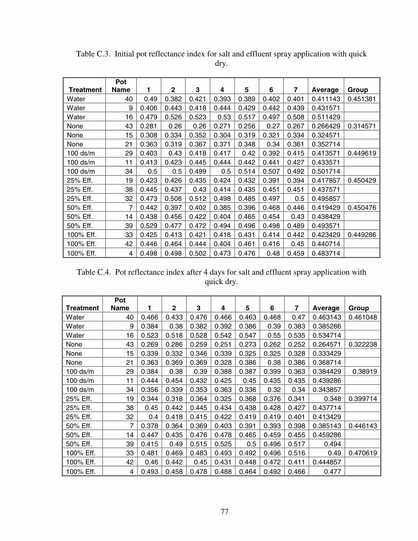
77

Table C.3. Initial pot reflectance index for salt and effluent spray application with quickdry.

TreatmentPot

Name 1 2 3 4 5 6 7 Average GroupWater 40 0.49 0.382 0.421 0.393 0.389 0.402 0.401 0.411143 0.451381Water 9 0.406 0.443 0.418 0.444 0.429 0.442 0.439 0.431571Water 16 0.479 0.526 0.523 0.53 0.517 0.497 0.508 0.511429None 43 0.281 0.26 0.26 0.271 0.256 0.27 0.267 0.266429 0.314571None 15 0.308 0.334 0.352 0.304 0.319 0.321 0.334 0.324571None 21 0.363 0.319 0.367 0.371 0.348 0.34 0.361 0.352714100 ds/m 29 0.403 0.43 0.418 0.417 0.42 0.392 0.415 0.413571 0.449619100 ds/m 11 0.413 0.423 0.445 0.444 0.442 0.441 0.427 0.433571100 ds/m 34 0.5 0.5 0.499 0.5 0.514 0.507 0.492 0.50171425% Eff. 19 0.423 0.426 0.435 0.424 0.432 0.391 0.394 0.417857 0.45042925% Eff. 38 0.445 0.437 0.43 0.414 0.435 0.451 0.451 0.43757125% Eff. 32 0.473 0.506 0.512 0.498 0.485 0.497 0.5 0.49585750% Eff. 7 0.442 0.397 0.402 0.385 0.396 0.468 0.446 0.419429 0.45047650% Eff. 14 0.438 0.456 0.422 0.404 0.465 0.454 0.43 0.43842950% Eff. 39 0.529 0.477 0.472 0.494 0.496 0.498 0.489 0.493571100% Eff. 33 0.425 0.413 0.421 0.418 0.431 0.414 0.442 0.423429 0.449286100% Eff. 42 0.446 0.464 0.444 0.404 0.461 0.416 0.45 0.440714100% Eff. 4 0.498 0.498 0.502 0.473 0.476 0.48 0.459 0.483714

Table C.4. Pot reflectance index after 4 days for salt and effluent spray application withquick dry.

TreatmentPot

Name 1 2 3 4 5 6 7 Average GroupWater 40 0.466 0.433 0.476 0.466 0.463 0.468 0.47 0.463143 0.461048Water 9 0.384 0.38 0.382 0.392 0.386 0.39 0.383 0.385286Water 16 0.523 0.518 0.528 0.542 0.547 0.55 0.535 0.534714None 43 0.269 0.286 0.259 0.251 0.273 0.262 0.252 0.264571 0.322238None 15 0.339 0.332 0.346 0.339 0.325 0.325 0.328 0.333429None 21 0.363 0.369 0.369 0.328 0.386 0.38 0.386 0.368714100 ds/m 29 0.384 0.38 0.39 0.388 0.387 0.399 0.363 0.384429 0.38919100 ds/m 11 0.444 0.454 0.432 0.425 0.45 0.435 0.435 0.439286100 ds/m 34 0.356 0.339 0.353 0.363 0.336 0.32 0.34 0.34385725% Eff. 19 0.344 0.318 0.364 0.325 0.368 0.376 0.341 0.348 0.39971425% Eff. 38 0.45 0.442 0.445 0.434 0.438 0.428 0.427 0.43771425% Eff. 32 0.4 0.418 0.415 0.422 0.419 0.419 0.401 0.41342950% Eff. 7 0.378 0.364 0.369 0.403 0.391 0.393 0.398 0.385143 0.44614350% Eff. 14 0.447 0.435 0.476 0.478 0.465 0.459 0.455 0.45928650% Eff. 39 0.415 0.49 0.515 0.525 0.5 0.496 0.517 0.494100% Eff. 33 0.481 0.469 0.483 0.493 0.492 0.496 0.516 0.49 0.470619100% Eff. 42 0.46 0.442 0.45 0.431 0.448 0.472 0.411 0.444857100% Eff. 4 0.493 0.458 0.478 0.488 0.464 0.492 0.466 0.477

78

Table C.1. Pot reflectance index after 1 week for salt and effluent spray application withquick dry.

TreatmentPot

Name 1 2 3 4 5 6 7 Average GroupWater 40 0.375 0.352 0.419 0.378 373 0.384 0.4 53.61543 18.1071Water 9 0.328 0.339 0.33 0.339 0.358 0.323 0.319 0.333714Water 16 0.376 0.362 0.366 0.405 0.352 0.381 0.363 0.372143None 43 0.241 0.26 0.244 0.239 0.234 0.245 0.248 0.244429 0.28019None 15 0.307 0.272 0.305 0.327 0.292 0.309 0.298 0.301429None 21 0.316 0.293 0.29 0.288 0.297 0.292 0.287 0.294714100 ds/m 29 0.31 0.317 0.311 0.289 0.301 0.295 0.318 0.305857 0.332100 ds/m 11 0.393 0.4 0.381 0.404 0.411 0.433 0.408 0.404286100 ds/m 34 0.288 0.3 0.283 0.298 0.27 0.285 0.277 0.28585725% Eff. 19 0.316 0.334 0.329 0.32 0.34 0.328 0.322 0.327 0.3571925% Eff. 38 0.375 0.381 0.411 0.388 0.377 0.389 0.402 0.38925% Eff. 32 0.363 0.355 0.347 0.366 0.368 0.329 0.361 0.35557150% Eff. 7 0.269 0.25 0.284 0.309 0.295 0.283 0.265 0.279286 0.37890550% Eff. 14 0.439 0.391 0.411 0.406 0.383 0.389 0.405 0.40342950% Eff. 39 0.477 0.445 0.441 0.459 0.442 0.478 0.436 0.454100% Eff. 33 0.398 0.409 0.404 0.406 0.39 0.411 0.4 0.402571 0.401714100% Eff. 42 0.399 0.337 0.36 0.389 0.356 0.358 0.371 0.367143100% Eff. 4 0.465 0.431 0.404 0.459 0.416 0.432 0.441 0.435429

Table C.1. Treatment characteristics for salt and effluent spray application with quickdry.

100% Eff. 50% Eff. 25% Eff. 100 ds/mDry Matter 0.80% 0.40% 0.20%EC ds/m 11.09 5.545 2.7725 100Soluable Salts (ppm) 7430 3715 1857.5 .051g NaCl/mlPhosphorus (P2O5) (ppm) 510.1 255.05 127.525Calcium (Ca) (ppm) 231.7 115.85 57.925Potassium (K2O) (ppm) 985.4 492.7 246.35Magnesium (Mg) (ppm) 125.8 62.9 31.45Sodium (Na) (ppm) 268.2 134.1 67.05Sulfur (S) (ppm) 112.2 56.1 28.05Iron (Fe) (ppm) 15.99 7.995 3.9975Zinc (Zn) (ppm) 8.69 4.345 2.1725Copper (Cu) (ppm) 1.28 0.64 0.32Manganese (Mn) (ppm) 3.29 1.645 0.8225Total C 0.45% 0.23% 0.11%Total N 0.12% 0.06% 0.03%

VITA

Spencer Lee Mann

Candidate for the Degree of

Master of Science

Thesis: THE TOLERANCE OF WW-IRON MASTER OLD WORLD BLUESTEM

TO SALINITY AND LAND-APPLICATION OF SWINE EFFLUENT

Major Field: Biosystems and Agricultural Engineering

Biographical:

Education: Received a Bachelor of Science degree in Biological Engineering

from Utah State University, Logan, Utah in May 2005. Completed the

requirements for the Master of Science degree with a major in Biosystems and

Agricultural Engineering at Oklahoma State University in July, 2007.

Experience: Gained valuable experience while working with anaerobic digestion

and biogas as an undergraduate at Utah State University. Additionally, worked

as a research engineer at the Swine Research Center at Oklahoma State

University for two years.

THE TOLERANCE OF WW -IRON MASTER OLDdigital.library.okstate.edu/etd/umi-okstate-2374.pdf · THE...

Documents

Transcript of THE TOLERANCE OF WW -IRON MASTER OLDdigital.library.okstate.edu/etd/umi-okstate-2374.pdf · THE...