The Tax Gradient:

Do Local Sales Taxes Reduce Tax Di�erentials at State Borders?

David R. Agrawal ∗

University of Michigan

This Version: November 11, 2011; Job Market Paper

Abstract

Geographic borders create a discontinuous tax treatment of retail sales and encourage

cross-border shopping by residents of high-tax states. But do municipalities' local

option taxes smooth these discontinuities? In a model where towns within a federation

maximize revenue and compete in a Nash game, equilibrium local tax rates decrease

from the nearest high-tax border and increase from the nearest low-tax border. Using

driving distance from the state border and data on all local sales tax rates in the United

States for 2010, I empirically test whether tax rates follow the pattern predicted by this

theoretical model. Local tax rates on the low-tax side of the border are signi�cantly

higher than on the high-tax side of the border, reducing the di�erential in state tax

rates at the border by more than half. Consistent with the model's prediction, a 100

mile increase in distance from the nearest high-tax border lowers local tax rates by 15%

of the average local rate. Local taxes fall most rapidly closest to the border and when

the di�erential in state tax rates is largest.

JEL: H21, H25, H73, H77, R12

Keywords: Sales Taxes, Cross-border Shopping, Tax Competition, Local Taxes, Borders,

Fiscal Federalism∗Contact information: University of Michigan Department of Economics, 611 Tappan Street, Ann Arbor,

MI 48109-1220. Email: dagrawal@umich.edu. I am especially grateful to my dissertation committee chair,Joel Slemrod, along with the members of my committee � David Albouy, Robert Franzese, James R. HinesJr. � for invaluable advice, encouragement, and mentoring. I also wish to thank Claudio Agostini, LeahBrooks (discussant), Charles Brown, Paul Courant, Lucas Davis, Michael Devereux (discussant), DhammikaDharmapala, Reid Dorsey-Palmateer, Michael Gideon, Makoto Hasegawa, William Hoyt (discussant), RaviKanbur, Sebastian Kessing, Miles Kimball, David Knapp, Michael Lovenheim (discussant), Olga Malkova,Ben Niu, Yulia Paramonova, Emmanuel Saez, Stephen Salant, Nathan Seegert, Daniel Silverman, Je�reySmith, Caroline Weber, and David Wildasin, as well as participants at the 2010 National Tax AssociationConference, the 2010 Michigan Tax Invitational, the Michigan Public Finance Seminar, Oxford University'sCentre for Business Taxation Doctoral Conference, and the 2011 International Institute of Public FinanceCongress, for helpful suggestions and discussions. I thank Pro Sales Tax for providing me access to proprietarydata. Special thanks to the International Institute of Public Finance for awarding this paper the Peggy andRichard Musgrave Prize. Any remaining errors are my own.

1 Introduction

The total sales tax rate in America ranges anywhere between 0% and 11%. Given these dis-

parities in tax rates, consumers may have large incentives to engage in cross-border shopping,

while �rms may have large incentives to locate on the low-tax side of borders. Geographic

borders create discontinuous changes in tax rates, which distort individual consumption and

�rm location decisions. Moreover, these discrete jumps in tax rates at borders may induce

towns to levy their sales tax based on an approximately continuous function of distance from

the border. This motivates my main question of interest: do localities assess local sales taxes

as a function of distance from the nearest state border, where tax rates decrease for localities

further from a higher-tax state, and increase for localities further from a lower-tax state?

Consider the example of high-tax California and low-tax Oregon. As a possible policy,

California could change taxes continuously and set lower taxes closer to the Oregon border.

This policy, in comparison to the uniform discontinuous case, would not change the e�ective

price of the good for consumers (including taxes and transportation costs), but may keep

extra revenue in California. However, a tax rate that is continuous in distance from the

border may have high administrative costs. Use of the local option sales tax may be an

administratively feasible way of obtaining a geographically di�erentiated pattern of sales tax

rates.

As a consequence of distortions from state tax competition, a municipality will set geo-

graphically di�erentiated tax rates depending on distance from the border. Therefore, the

spatial arrangement of jurisdictions determines the strategic nature of local tax competition.

Intuitively, the spatial arrangement matters because state borders in�uence the elasticity of

demand with respect to prices. Local jurisdictions with a lower elasticity of demand will set

higher tax rates. In the presence of discontinuous changes in state tax rates at borders, on

the low-tax side, jurisdictions near the border realize a smaller elasticity of demand because

the in�ow of cross-state shoppers augments their tax base. On the high-tax side, the elas-

ticity of demand is larger for jurisdictions near the border because the out�ow of cross-state

shoppers reduces the tax base.

In the context of a theoretical model that expands several elements from Kanbur and

Keen (1993), I demonstrate that from the local government's perspective, the equilibrium

tax rates in a federal system depend on the distance of each jurisdiction to a neighboring

state. This contrasts with the existing tax competition literature, which has focused on

the role of jurisdiction size as a determinant of tax rates and has generally concluded that

if jurisdictions are the same in all characteristics, they will select the same tax rate. The

model in this paper provides a novel insight that the spatial characteristics of towns � distance

2

from the border and the size of the discontinuity in state tax rates at the border � within a

federation determine tax rates. Given varying public good preferences across states, a broad

uniform tax rate within the federation will not occur in equilibrium if sub-state governments

exist � even if all of the sub-federal governments are identical in every respect except spatial

arrangement.

The theoretical model yields four testable results. First, in a local region of the border,

municipal sales taxes on the low-tax side of the border are higher than municipal taxes on the

high-tax side of the border. Second, on the relatively low-tax side of the border, municipal

taxes decrease as towns are further from the border; on the relatively high-tax side of the

border, local taxes increase as towns are further from the border. I refer to the pattern

(slope) of local option taxes, moving away from the border, as the �tax gradient.� Third,

local taxes rise or fall most rapidly in the vicinity of the state border. That means that the

tax gradient is steepest in the vicinity of the border. Fourth, the size of the discontinuity

a�ects the slope of the tax gradient. The tax gradient is steeper when the di�erential in

state tax rates is larger.

Empirically, the paper examines whether localities with the option to assess local sales

taxes set their tax rate in a manner consistent with the four theoretical propositions above.

The methodology outlined in the paper will be applicable to research on how jurisdictions

respond to any policy (e.g., environmental, labor) that varies discontinuously at the state

border. The paper uses a previously unused and comprehensive data set of all local sales

tax rates in the United States � municipal, county, and district rates. I also have created

an accurate and detailed data set of spatial proximity to borders. I �nd the shortest driving

distance from the population centroid of each town to a state-border major road crossing,

in order to accurately measure how towns set tax rates away from the border. This distance

minimizes measurement error in the actual distance a consumer would travel to cross-border

shop.

First, I �nd that local tax rates on the low-tax side of the border are signi�cantly higher

than on the high-tax side of the border, reducing the di�erential in state tax rates at the

border by more than half. Ignoring local option taxes, the average di�erential in state tax

rates is 1.9 percentage points. After accounting for all local option taxes, the tax di�erential

at state borders decreases by 1.2 percentage points. Second, the average marginal e�ect of

distance on the local (municipal plus sub-district) tax rate in a jurisdiction is signi�cantly

negative and of the expected sign on the low-tax side. The marginal e�ect of distance is

robust to controlling for distance from the second closest state border and the distance from

county borders. A 100 mile increase in distance from the nearest high-tax border lowers local

tax rates by 15% of the average local rate. Third, taxes fall most rapidly in a local region of

3

the border. Fourth, taxes fall more rapidly if the tax di�erential in state tax rates is larger.

This paper will proceed as follows. After presenting background on local option taxes,

I develop a model where multiple town governments face pressures from tax di�erentials at

multiple state borders and choose the local tax rates in order to maximize revenue in the

town. I show that in a Nash equilibrium, local tax rates depend on the distance from a

state border. I test this theoretical result in the empirical analysis. Given that the system of

local option sales taxes in the United States approximates the theoretical model, I evaluate

whether such a relationship between tax rates and distance from the state border exists in the

data using a global polynomial regression design. Finally, I discuss the welfare implications

of the policy and o�er some concluding thoughts.

2 Background

In this section, I review the standard tax competition literature that my model will build

upon. I also review current studies that have incorporated a role for distance from the border

in their empirical or theoretical analysis of cross-border shopping. Finally, I provide policy

background on local taxes and how they vary across states.

2.1 Comparison to the Existing Literature

2.1.1 Tax Competition and Distance

Previous literature on tax competition tries to explain asymmetries in tax rates among com-

peting jurisdictions when each jurisdiction chooses a uniform tax rate within its boundaries.

The approach to solving this problem has varied substantially. Kanbur and Keen (1993)

develops a model with a single good in partial equilibrium where governments are revenue

maximizers. Nielsen (2001) extends Kanbur and Keen (1993) to welfare maximizing gov-

ernments, but relies on an additively separable relationship between consumer surplus and

revenue. Hoyt (2001) studies the optimality of sales taxes within a federation.

The conclusions from these models highlight the way jurisdictions may reach an equilib-

rium with di�erent tax rates. Hau�er (1996) implies that a state like California may have

higher tax rates than Oregon because of stronger preferences for public goods. This is in

contrast to models such as Bucovetsky (1991), Kanbur and Keen (1993), Nielsen (2001), and

Trandel (1994), which focus on country size or population as an explanation for variation

in tax rates and �nd that larger jurisdictions set higher rates. This paper uses the result

that tax di�erentials will exist at state borders as a starting point. The model proposed in

my paper will extend Kanbur and Keen (1993) by incorporating multiple competitors and

4

distance from the border as an explanation for tax di�erences within states. My model will

help to explain responses of jurisdictions to tax notches, which according to Slemrod (2010)

are widespread in any federalist tax system.

Recently, several studies have focused on the role of distance to a competing jurisdiction,

which will be a key variable in this paper. Lovenheim (2008) studies how distance from the

nearest lower-tax cigarette state relates to the demand elasticity of home state consumption.

He �nds that cigarette demand becomes more elastic to the home state price the further

individuals live from a lower price cigarette border because the cost to obtain a given amount

of saving rises. This implies that cross-border shopping is most problematic for border

localities.1 In a similar light, Harding, Leibtag and Lovenheim (Forthcoming) �nd that

the incidence of taxation varies depending on a �rm's distance from the nearest lower-tax

border. Both papers �nd that the nearest low-tax border is the only border which results

in any geographic di�erentiation. Merriman (2010) also analyzes distance from the border

and shows the likelihood of having an Indiana cigarette tax stamp (the low-tax neighboring

state to Illinois) is decreasing in the distance from the Indiana border. The results from these

papers clearly indicate that distance from the border shapes the responsiveness of individuals

to cross-border shop.

2.1.2 Competition Among Localities

Many studies have analyzed how local sales taxes in�uence cross-border shopping with little

emphasis on the geographic distribution of these local sales tax rates within a state. Em-

pirically, a large literature attempts to quantify the price responsiveness of consumers to

state border e�ects. The �ndings suggest that a 1% increase in a sales tax rate results in a

1% to 6% reduction in sales, although the geographic unit of analysis varies across di�erent

studies (Mikesell 1970; Fox 1986; Walsh and Jones 1988; Tosun and Skidmore 2007). This

behavioral response is indicative of the degree of cross-border shopping and will play an

important role in the following model.

The behavioral response is also important to determine with whom localities compete.

Using data on local sales tax rates in Tennessee, Luna (2003) demonstrates that the sales

tax rates in neighboring states in�uence the tax rate that a local government selects, both in

the long run and in the short run. Similar inter-dependencies are found in Georgia (Sjoquist

et al. 2007). However, Luna, Bruce and Hawkins (2007) �nd that a jurisdiction does not

decide to reach the maximum statutory rate based on its neighbors' decisions to do so.

1Using a similar methodology, Lovenheim and Slemrod (2010) studies the e�ect of having a neighboringcounty with a lower minimum legal drinking age on the number of accident fatalities.

5

2.1.3 Summary

Although the location of state borders are not chosen as a matter of policy, geographic

borders between di�erent states create a discontinuous tax policy. State borders are an

example of a �line� in the tax system. The line creates a �notch� � or a discontinuous jump

in the tax rate of the good based on the characteristics of the good � where the characteristic

of the good is the location of purchase.

The existing literature indicates that competition over sales will naturally result in tax

�notches� at state borders, but has ignored how localities will respond to these di�erentials.

Given that these di�erentials arise, the empirical literature indicates cross-border shopping

is highly elastic to tax rate changes. But, the responsiveness of cross-border shopping is

empirically not uniform in a state, resulting in larger responses closer to the border. In light

of this, local option taxes may provide a mechanism for smoothing tax di�erentials, which

result in cross-border shopping and distorted �rm location choices at state borders.

2.2 Background on the Local Option Sales Tax

Local option sales taxes (LOST) are widely used in the United States. Of the forty-�ve

states that impose a sales tax ranging between 2.9% and 7%, thirty-six allow local or county

governments to set LOST. Over 7,500 localities utilize this option. Among these towns, the

local sales tax contributed anywhere from 1% to 52.2% of municipalities' revenues during

�scal year 2006 (Mikesell 2010). Sales taxes in the United States are levied de facto according

to the origin principle.2 This implies that the jurisdiction of sale rather than the jurisdiction

of residence e�ectively determines the tax paid.

There is substantial variation in the way the local option sales tax works.3 Fourteen

states do not allow for LOST. Of the remaining states that allow for LOST, the locality's

degree of autonomy varies greatly. For example, the smallest unit that is granted autonomy

to assess a tax varies from the county level (example: Wyoming) to the town level (most

states), to within-town jurisdictions such as �re, school or transportation districts (examples:

Colorado or Georgia). Of states that allow municipalities to set a tax, some do not allow

counties to assess an additional tax (example: South Dakota), although most do. In other

2When an individual cross-border shops, the sales tax is paid in the jurisdiction of purchase. However,the individual is legally responsible for �ling a use tax � the excise tax on purchases of items for whichthe home state's sales tax was not previously paid � in the state of residence. The use tax is notoriouslyunder-enforced. Because the use tax is often evaded, taxes are implicitly paid based on the sales tax and,therefore, are based on the origin of the purchase rather than the destination of the sale.

3All of the descriptions in this section come from my own review of the Department of Revenue sitesfor each state. The Guide to Sales and Use Taxes (Research Institute of America 2010) also providesstate-by-state information on state sales taxes.

6

states, a mandatory county rate is set uniformly across the state with the option to increase

the rate (example: California). Some consumers face di�erent tax rates street blocks away

while others need to travel more than 50 miles before the tax rate changes.

States also vary in terms of how the tax base is de�ned. Lines are drawn on what goods

are taxed under the retail sales tax. In most states, the de�nition of the tax base at the

state level is the base that applies to LOST. Some exceptions exist. For example, in the state

of Florida, only the �rst $5,000 of a purchase is taxable under LOST. Other states impose

restrictions on the rate increases that localities can impose at any given time. For example,

counties in Ohio can only select taxes in increments of 1/4 of a percentage point and the

maximum rate a county can assess is capped (at a fairly high rate). On the other hand, the

maximum LOST in Iowa is capped at 1 percentage point, so �maxing out� is common.

The method in which localities determine whether to implement LOST and the rate at

which to set it also varies by state. In most states, only a city or town government needs

to pass LOST. In other states, such as Iowa, the process is more complicated. In Iowa, a

referendum determines LOST. Voters determine the rate of the tax, the purpose of the tax,

and the sunset provisions on the tax. North Carolina, on the other hand, requires approval

of the state legislature for LOST rates. The method of collection also varies; businesses remit

taxes directly to the state or the locality, depending on the state.

Finally, two states allow local jurisdictions to set implicitly negative tax rates. Within

Urban Enterprise Zones in New Jersey and Empire Zones in New York, localities may set tax

rates lower than the state tax rate at no revenue cost to the locality. In fact, some locations

elect to implement the favorable rate.

3 Theory of Local Competition with Heterogeneous States

In this section, I develop a model to evaluate the equilibrium commodity tax rates when

local jurisdictions can assess a local sales tax. The goal of this model is to show that the

equilibrium local sales tax rates are not uniform within a state � even if the towns are

identical in preferences and size.

My paper extends Kanbur and Keen (1993)'s two-state partial equilibrium model of cross-

border shopping by allowing for multiple jurisdictions and multiple levels of government.

Compared to standard models, I place jurisdictions on a Salop Circle rather than a Hotelling

line so that all jurisdictions have two neighbors.

7

3.1 Setup of the Model

The model features three states located on a circle that are indexed by j = H, M, L for high-,

medium-, and low-tax states.4 Each state has three identical towns5 indexed i = A, B, BB,

where I arrange the towns along the circumference of a circle as depicted in Figure 1. �A�

denotes the towns �Away� from the border. �B� and �BB� denote the towns close to the

�Border� in their respective states. Each town is of equal length and each town covers a

distance of x units along the line segment.

Modeling jurisdictions on a circle rather than a line has important implications. On a line

segment, the towns furthest away from the state border have only one neighbor rather than

two by virtue of their position at the end of the line segment. The purpose of this model is to

determine � from a town government's perspective � the pattern of geographic di�erentiation

resulting from the notch at the state border. When considering such a problem, the local

government will take into account the town's position along the line segment, which includes

both the number of towns away from the state border and the number of borders with other

towns. Therefore, if I use a line segment in the model, towns on the exterior of the line will

possibly have di�erent rates for two reasons � one, because they are far from the state border

and two, because they can only undercut one town rather than two and therefore have a

di�erent elasticity. However, all the variation in the tax rates is a result of distance from

the border and not from the number of neighbors present, when I place the states along the

circumference of a circle.6

The model has three agents: producers, consumers, and governments. I assume �rms

providing one private consumption good locate exogenously at any point along the circle's

circumference. Firms are perfectly competitive and set price equal to marginal cost. When

purchases at a particular point along the circle are high, more stores enter. Although the

distribution of stores need not be uniform, �rms are simply responding to consumption deci-

sions; �rms do not manipulate cross-border shopping. The implication of perfect competition

is that increases in the demand of a good in a particular town � resulting from cross-border

shopping � will not alter the pre-tax price relative to the pre-tax price in another town. Nor

will taxes alter the pre-tax price. Therefore, the pre-tax price is the same in all jurisdictions

and is normalized to one.7

State governments levy a state sales tax rate, τ j, on commodity purchases within the

4A two state-model is available online at http://www-personal.umich.edu/~dagrawal/research.htm.5The towns could be equally sized sub-regions. The word �town� only need imply a governing entity.6Of course, the linear model may be more descriptive to some states. One example is Florida, where the

northern border touches two states. The Florida peninsula is surrounded entirely by ocean water, whichimplies that there are many Florida towns that are likely to have �one� less neighbor.

7The model assumes the incidence of the tax is fully passed forward to consumers as well.

8

state. In this analysis, I assume that state tax rates are exogenous and known to all localities

before localities compete over taxes.8 Exogenously di�erent preferences for a state public

good will imply that the state tax rates will di�er across the states.9 State H sets the highest

tax rate and State L sets the lowest tax rate. State M has a rate in between the other two

rates such that τH > τM > τL. Denote S = τM − τL, R = τH − τM , and D = τH − τL

so that it measures the size of the �notch� induced by the state tax di�erential. Note that

because states are around a circle, it must be that D = S + R. Town governments i in

state j levy local taxes on the consumption good at rate tji .10 Taxes are assessed under

the origin principle so that the location of purchase de�nes the tax rate that the consumer

pays. Denote the sum of the state and local tax rate in jurisdiction i of state j as T ji so

T ji = τ j + tji . Towns compete in a Nash game over the local sales tax rates. The objective

of the local government is to maximize the tax revenue it raises from the local tax on the

consumption goods purchased within its town borders.11

Consumers are distributed uniformly across each town and the populations are identical

in all towns. Consumers cannot migrate. Demand is perfectly inelastic. Each consumer

will purchase one unit of the consumption good, but will have a choice over the location of

purchase and can travel along the circumference of the circle to do so. Transportation costs

make purchasing goods in another jurisdiction less bene�cial.

Let V denote the reservation value net of the producer price for each consumer. V is

8The explicit assumption requires that tax competition over local sales tax rates has no e�ect on equi-librium state sales tax rates. The intuition for this is that most localities in the United States are small.Therefore, small changes in the local tax rates should not induce a response in the state sales tax rates.Of course, changes in large city tax rates may violate this assumption. An alternative model would be onewhere states are Stackelberg leaders.

9All states are the same in size and population density. Hau�er (1996) shows that di�erences in preferencesfor the public good are an alternative explanation for varying tax rates in equilibrium. I assume that theseexogenously di�erent preferences for state public goods result in di�erent state tax rates, but make no furtheruse of this assumption.

10The model assumes governments only have access to a sales tax. If other tax instruments were available,the results below would be similar so long as governments rely on sales taxes to some extent.

11An alternative to modeling revenue maximizing governments is to model welfare maximizing govern-ments. If governments maximize welfare, the government will care not only about the revenue raised, butalso the amount of the consumption good its residents can purchase. Revenue maximizing governments canbe interpreted in several ways. The solution to the problem of revenue maximizing governments approximatesthe solution to welfare maximizing governments when consumers have a high marginal value of the publicgood �nanced by the government. Second, so long as borders are open, the solution for revenue maximizinggovernments will approximate the welfare maximizing government's solution when the marginal utility ofconsumption is constant (which will be the case when the utility function of the individual is quasi-linear inconsumption). Linearity in the consumption good seems to be a realistic assumption for cross-border shop-ping, which often results in many purchases of a few similar items. I use revenue maximizing governmentsin my model because the introduction of multiple towns and levels of government complicates the alreadycomplex problem of two competing jurisdictions and I need this simplifying assumption to make the modeltractable.

9

assumed to be large enough so that all consumers either purchase one unit of the good from

their home town or elsewhere. If the individual decides to purchase in the home town, she

simply goes to the store at the point of the circle corresponding to where she lives and does

not incur any transportation costs. If the consumer elects to do this, she purchases the

good for a price equal to the tax-inclusive marginal cost of production. The surplus she will

receive from such a purchase is V − T ji .Alternatively, each consumer can purchase the consumption good elsewhere.12 If she

elects to do so, she will drive along the circumference to the nearest town border and purchase

the good from the store located exactly at the border. Let the distance to the nearest town

border for any consumer be denoted s. The transportation cost of traveling to the border

(and back) is denoted δ > 0 per unit of travel. The surplus the consumer will receive from

purchasing one unit of the private good abroad is V − T lk − δs, where k 6= i indexes the tax

rate in a foreign town of state l, which may be equal to j if she does not cross state lines.

A consumer will purchase the private good from the neighboring town if the surplus of

purchasing the good is strictly greater than zero and if the surplus from buying the good

elsewhere is strictly greater than buying the good at home. Comparing the consumer surplus

from purchasing the good elsewhere with the surplus from purchasing the good from home,

it is evident that a consumer will purchase the good elsewhere if:

T ji − T lkδ

> s for T ji > T lk. (1)

The implication of Equation 1 is that all residents who live farther thanT ji −T

lk

δunits from a

low-tax border will purchase the good at home, while all other consumers cross-border shop

in the nearest low-tax jurisdiction. The model assumes that x is su�ciently large so that

towns do not have incentives to target consumers multiple towns over.13

12In reality, individuals also have the option to purchase goods on the Internet and completely evade taxes.As long as some people in each state still cross-border shop and the use of the internet does not vary bytown, all the results of the model will carry through. The presence of an Internet with tax-free purchaseswill only a�ect the number of people cross-border shopping and the relative slopes of local tax rates, but thequalitative pattern will be the same.

13The assumption of shopping no more than one town over simpli�es the nature of the problem, but wouldnot change the qualitative results. Relaxing this assumption would require checking incentive constraints onthe individual for all towns to which cross-border shopping is feasible. The assumption of a linear transportcost and a su�ciently large x rules out this possibility. Intuitively, relaxing this assumption would reducethe degree of geographic di�erentiation and the level of local tax rates as towns will compete over the taxrates more aggressively.

10

3.2 Benchmark Solutions

Given the assumptions outlined above, it is easy to see that each town government will

extract all the surplus from its residents in equilibrium if all borders are closed or if a use tax

could be perfectly enforced. Therefore, the equilibrium tax rates will be to set tji = V − τ j

for i = A,B,BB in j = L,M,H. If all states have equal state tax rates and borders are

open, the equilibrium local tax rates would not be geographically di�erentiated and would

be characterized by tji = δx for all i. This contrasts with a model where towns are located

along a line segment. Along a line segment, the Nash equilibrium is for Town A to set local

tax rates that are 4/5 of the level of the tax rates at the extremity because of their ability to

undercut two towns rather than one. If all state taxes are uniform or if all town borders are

closed (e.g., use taxes are perfectly enforced), the equilibrium town tax rates are uniform

within a state.14

3.3 Equilibrium with Three Heterogeneous States

It is essential to know the direction of cross-border shopping to solve the model. Recall that

although the state rates are exogenous, the towns within the state are free to set whatever

tax rate they desire. I consider all possible patterns of local option taxes along the circle;

taxes increase from borders, decrease from borders, or taxes are random. I must also allow

for the possibility that after local option taxes are assessed, the total tax rate on the low-tax

side of the border may be higher than on the high-tax side.

The revenue for each town can be derived using Equation 1. The tax base is de�ned as

the total number of consumers within a town i of state j minus those individuals in that

town who shop elsewhere plus individuals from other towns who shop in i. Multiplying the

tax base by tji yields total revenue and the municipality maximizes total revenue by selecting

tji . The best response functions are linear and will be continuous when changing from a

high- to a low-tax jurisdiction. This continuity as towns change regimes implies that one

set of best response functions characterizes the equilibria for all possible cases � including

non-symmetric cases.

The revenue functions for towns in State M are de�ned in Equation 2. The revenue

14International borders are much more likely to be �closed� to cross-border shopping. Transportationcosts, broadly de�ned, are much higher for crossing an international border. International borders usuallytake more time to cross, have some probability of vehicle search, and require individuals to exchange theircurrency before they can purchase goods abroad.

11

functions for State H and L are omitted for simplicity, but are de�ned in a similar manner.

RMi =

tMA (x+

tMBB−tMA

δ+

tMB −tMA

δ)

tMBB(x+tHB−t

MBB+R

δ+

tMA −tMBB

δ

tMB (x+tLBB−t

MB −Sδ

+tMA −t

MB

δ)

)

for Town A

for Town BB

for Town B.

(2)

Notice that xtji denotes the revenue in the absence of cross-border shopping. The second

and third terms represent the in- and out-�ows resulting from cross-border shopping with

both neighbors. If these terms are positive, then cross-border shopping is inward. If they are

negative, cross-border shopping is outward. If the neighboring state is a high-tax state, the

discontinuity in tax rates enters positively, but if the neighboring state is a low-tax state,

the di�erential in the state tax rates enters negatively.Solving the problem by di�erentiating the revenue functions yields the following best

response functions:

tHBB(·) = 14 (δx− (R+ S) + tHA + tLB) tHA (·) = 1

4 (δx+ tHBB + tHB ) tHB (·) = 14 (δx−R+ tHA + tMBB)

tMBB(·) = 14 (δx+R+ tHB + tMA ) tMA (·) = 1

4 (δx+ tMBB + tMB ) tMB (·) = 14 (δx− S + tMA + tLBB)

tLBB(·) = 14 (δx+ S + tMB + tLA) tLA(·) = 1

4 (δx+ tLBB + tLB) tLB(·) = 14 (δx+ (R+ S) + tHBB + tLA),

(3)

which imply that municipality i's neighboring local tax rates are strategic complements, but

that tji and τj are strategic substitutes.

Solving this system of equations for a Nash equilibrium yields the following results:

tHBB = κ(ω − 12R− 11S) tHA = κ(ω − 6R− 3S) tHB = κ(ω − 12R− S)

tMBB = κ(ω + 11R− S) tMA = κ(ω + 3R− 3S) tMB = κ(ω +R− 11S)

tLBB = κ(ω +R + 12S) tLA = κ(ω + 3R + 6S) tLB = κ(ω + 11R + 12S),

(4)

where κ = 1/53 and ω = 53δx/2. The �rst section of the Appendix proves that the Nash

equilibrium derived above is unique for a general number of states and towns.

Di�erencing the local tax rates on the high- and low-tax side of borders shows that border

towns in a low-tax state will set relatively higher tax rates than border towns within a high-

tax state. The di�erential in tax rates at the state border shrinks to 3053

of the di�erential

when there is no competition over local option taxes and this pattern holds for all three

discontinuities.

To determine if the Nash equilibrium exists and its pattern, I need to verify three con-

ditions. First, I need to verify that T ji is larger on the high-tax side of the border in any

equilibrium and that all taxes are positive. Second, I need to determine the direction of the

inequality between tjA T tjB and tjA T tjBB for all states. Finally, I need to verify whether the

12

direction of these inequalities is consistent with the assumption that cross-border shopping

occurs only one town over along the continuum. For a Nash equilibrium to exist, I must also

verify that the number of residents of each town that cross-border shop is strictly less than

the total population of the town.

From Equation 4, the Nash equilibrium will always have the following properties: tHA >

tHBB, tMBB > tMA > tMBB, and t

LB > tLA. The intuition of this result is explained below. However,

in a Nash equilibrium, tHA T tHB and tLA T tLBB. The direction of these inequalities depends on

the relative sizes of the model's parameters � speci�cally the di�erentials in state tax rates.

It can be shown that tHA > tHB if R > 14D and tLBB > tLA if S > 1

4D. If the reverse is true then

the pattern of those two tax rates will �ip. It is also easy to verify that total taxes, T ji , on

the high-tax side of the border are always greater than total taxes on the low-tax side of the

border in equilibrium.

For a Nash equilibrium to exist, I must �nd the size of each town that guarantees that

tax rates are strictly positive, all towns have some residents that shop at home, and that no

one will shop more than one town away.15 Denoting the value of x that satis�es all three

of these conditions as x∗, a Nash equilibrium exists in pure strategies so long as x > x∗.

Strictly positive tax rates can be guaranteed by setting x > κ22D+2Rδ

. Verifying that no one

shops more than one town over and that some shoppers purchase the good at home requires

x > κ30Dδ> κ22D+2R

δ. Therefore, this guarantees that a small deviation in the tax rate of a

particular town cannot change revenues discontinuously. Thus, x > κ30Dδ

guarantees these

assumptions hold. If x < κ30Dδ, then no Nash equilibrium exists in pure strategies. But,

x > κ30Dδ, combined with continuity and concavity of the best response functions in the

strategies, guarantees the existence of the unique Nash equilibrium described above.

After de�ning two terms, I can state a proposition that characterizes the Nash equilibrium

for a general model with many towns.

De�nition. The tax gradient is de�ned as the slope of local option taxes away from the

border. De�ne the distance of a town to its relevant state border as the length along the

circumference from the center of the town to the relevant state border. Then, the tax gradient

is increasing in distance from the border if local option taxes increase as towns are further

from the relevant state border. The tax gradient is decreasing in distance from the border if

local option taxes decrease as towns are further from the relevant state border.

In the presence of multiple borders, the gradient will likely switch slopes at some point

within the state.

15This is equivalent to �nding a value of δ that is su�ciently large.

13

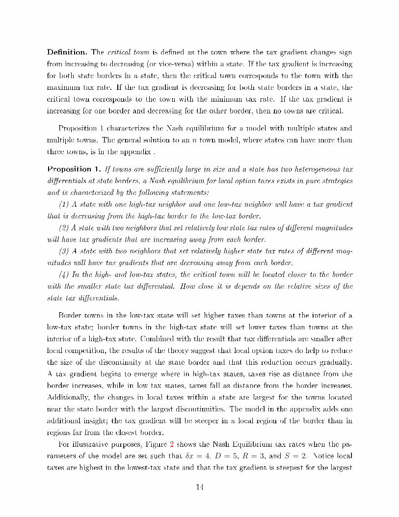
De�nition. The critical town is de�ned as the town where the tax gradient changes sign

from increasing to decreasing (or vice-versa) within a state. If the tax gradient is increasing

for both state borders in a state, then the critical town corresponds to the town with the

maximum tax rate. If the tax gradient is decreasing for both state borders in a state, the

critical town corresponds to the town with the minimum tax rate. If the tax gradient is

increasing for one border and decreasing for the other border, then no towns are critical.

Proposition 1 characterizes the Nash equilibrium for a model with multiple states and

multiple towns. The general solution to an n town model, where states can have more than

three towns, is in the appendix .

Proposition 1. If towns are su�ciently large in size and a state has two heterogeneous tax

di�erentials at state borders, a Nash equilibrium for local option taxes exists in pure strategies

and is characterized by the following statements:

(1) A state with one high-tax neighbor and one low-tax neighbor will have a tax gradient

that is decreasing from the high-tax border to the low-tax border.

(2) A state with two neighbors that set relatively low state tax rates of di�erent magnitudes

will have tax gradients that are increasing away from each border.

(3) A state with two neighbors that set relatively higher state tax rates of di�erent mag-

nitudes will have tax gradients that are decreasing away from each border.

(4) In the high- and low-tax states, the critical town will be located closer to the border

with the smaller state tax di�erential. How close it is depends on the relative sizes of the

state tax di�erentials.

Border towns in the low-tax state will set higher taxes than towns at the interior of a

low-tax state; border towns in the high-tax state will set lower taxes than towns at the

interior of a high-tax state. Combined with the result that tax di�erentials are smaller after

local competition, the results of the theory suggest that local option taxes do help to reduce

the size of the discontinuity at the state border and that this reduction occurs gradually.

A tax gradient begins to emerge where in high-tax states, taxes rise as distance from the

border increases, while in low-tax states, taxes fall as distance from the border increases.

Additionally, the changes in local taxes within a state are largest for the towns located

near the state border with the largest discontinuities. The model in the appendix adds one

additional insight; the tax gradient will be steeper in a local region of the border than in

regions far from the closest border.

For illustrative purposes, Figure 2 shows the Nash Equilibrium tax rates when the pa-

rameters of the model are set such that δx = 4, D = 5, R = 3, and S = 2. Notice local

taxes are highest in the lowest-tax state and that the tax gradient is steepest for the largest

14

discontinuities. For the three state, nine town model, the solution can be characterized as

follows. If x < x∗, then no Nash equilibrium exists in pure strategies. If x > x∗, the Nash

equilibrium will have tHA > tHBB, tMBB > tMA > tMBB, and t

LB > tLA with the relationship between

tHA , tHB and tLA, t

LB determined by the relative sizes of the notches given above.

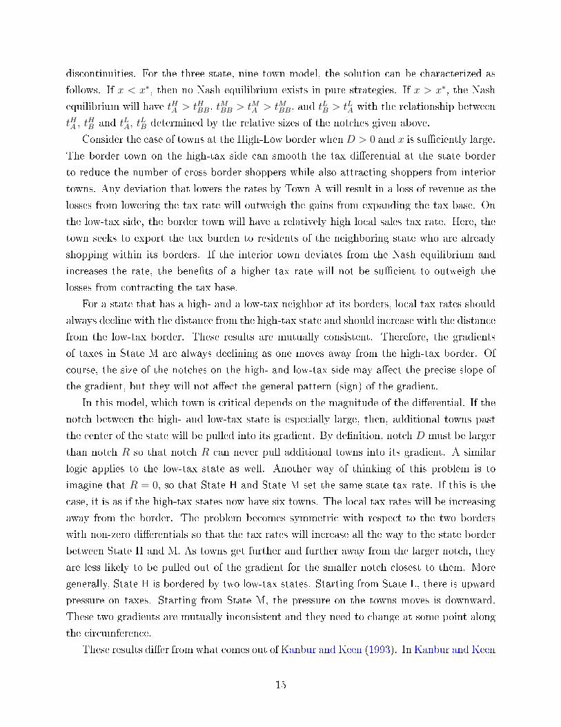
Consider the case of towns at the High-Low border when D > 0 and x is su�ciently large.

The border town on the high-tax side can smooth the tax di�erential at the state border

to reduce the number of cross-border shoppers while also attracting shoppers from interior

towns. Any deviation that lowers the rates by Town A will result in a loss of revenue as the

losses from lowering the tax rate will outweigh the gains from expanding the tax base. On

the low-tax side, the border town will have a relatively high local sales tax rate. Here, the

town seeks to export the tax burden to residents of the neighboring state who are already

shopping within its borders. If the interior town deviates from the Nash equilibrium and

increases the rate, the bene�ts of a higher tax rate will not be su�cient to outweigh the

losses from contracting the tax base.

For a state that has a high- and a low-tax neighbor at its borders, local tax rates should

always decline with the distance from the high-tax state and should increase with the distance

from the low-tax border. These results are mutually consistent. Therefore, the gradients

of taxes in State M are always declining as one moves away from the high-tax border. Of

course, the size of the notches on the high- and low-tax side may a�ect the precise slope of

the gradient, but they will not a�ect the general pattern (sign) of the gradient.

In this model, which town is critical depends on the magnitude of the di�erential. If the

notch between the high- and low-tax state is especially large, then, additional towns past

the center of the state will be pulled into its gradient. By de�nition, notch D must be larger

than notch R so that notch R can never pull additional towns into its gradient. A similar

logic applies to the low-tax state as well. Another way of thinking of this problem is to

imagine that R = 0, so that State H and State M set the same state tax rate. If this is the

case, it is as if the high-tax states now have six towns. The local tax rates will be increasing

away from the border. The problem becomes symmetric with respect to the two borders

with non-zero di�erentials so that the tax rates will increase all the way to the state border

between State H and M. As towns get further and further away from the larger notch, they

are less likely to be pulled out of the gradient for the smaller notch closest to them. More

generally, State H is bordered by two low-tax states. Starting from State L, there is upward

pressure on taxes. Starting from State M, the pressure on the towns moves is downward.

These two gradients are mutually inconsistent and they need to change at some point along

the circumference.

These results di�er from what comes out of Kanbur and Keen (1993). In Kanbur and Keen

15

(1993), the �small� country, as de�ned by domestic population, always undercuts the large

country in a Nash equilibrium. In the model I present above, towns set taxes following an

inverse elasticity rule,16 but what matters is the relative size of the �foreign� plus �domestic�

market. For Town BB in State H, even if its local tax rate is zero, some residents will always

shop abroad. Therefore, starting from a position where tHBB = tHA > 0, Town BB perceives a

relatively small (in comparison to Town A) market of �foreign� plus �domestic� shoppers (it

already has some of its residents shopping in the neighboring state, which reduces its market

size). Town BB perceives the relatively larger elasticity (because its market is smaller) and

undercuts Town A. On the low-tax side, starting from tLB = tLA > 0, Town B is already

attracting residents from the neighboring states. Therefore, because of the fact that B has

already attracted some foreign residents, it perceives the �foreign� plus �domestic� market

as larger than that of A. Town A perceives itself as small and undercuts Town B. Thus, the

town with the the largest cumulative �foreign� plus �domestic� market will always set higher

rates.

The theoretical model discussed above has several testable hypotheses for the empirical

analysis to follow. First, municipal tax rates are lower on the high-tax side of the state border

than on the low-tax side of the border. Second, local tax rates are decreasing away from the

nearest high-tax border and are increasing away from the nearest low-tax border. Third, the

distance of the municipality from the state border will determine how steep the tax gradient

is. The treatment e�ect will be heterogeneous by distance, because the tax gradient will

be steepest for the towns closest to the state border. Fourth, the size of the notch will

determine how steep the tax gradient is. For larger discontinuities in state tax rates, the tax

gradient will become steepest. This suggests that the treatment must be continuous (as a

function of the size of the notch) rather than a simple binary treatment for high- or low-tax

states. In addition, the theory implies that the critical town will depend on the relative size

of the discontinuities at various borders. This suggests that it is important to account for

the presence of multiple borders in the regression equations. Finally, the existence of a tax

gradient may be tested in other contexts; the theory will also apply to county borders.

4 Data and Evidence on the Levels of Local Tax Rates

The goal of the analysis is twofold. One, do localities on the high-tax side of a border set

lower local taxes than localities on the low-tax side? Two, is there a tax gradient that is a

16Put di�erently, one needs to set the tax rate inversely proportional to the elasticity of demand tomaximize revenue from a tax on sales. Here, the elasticity of demand is derived from cross-border shopping.When the elasticity of cross-border shopping is high, the town has an incentive to undercut the other town.

16

function of distance from the border?

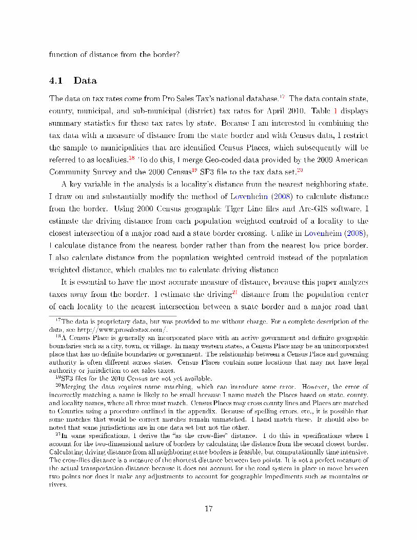
4.1 Data

The data on tax rates come from Pro Sales Tax's national database.17 The data contain state,

county, municipal, and sub-municipal (district) tax rates for April 2010. Table 1 displays

summary statistics for these tax rates by state. Because I am interested in combining the

tax data with a measure of distance from the state border and with Census data, I restrict

the sample to municipalities that are identi�ed Census Places, which subsequently will be

referred to as localities.18 To do this, I merge Geo-coded data provided by the 2009 American

Community Survey and the 2000 Census19 SF3 �le to the tax data set.20

A key variable in the analysis is a locality's distance from the nearest neighboring state.

I draw on and substantially modify the method of Lovenheim (2008) to calculate distance

from the border. Using 2000 Census geographic Tiger Line �les and Arc-GIS software, I

estimate the driving distance from each population weighted centroid of a locality to the

closest intersection of a major road and a state border crossing. Unlike in Lovenheim (2008),

I calculate distance from the nearest border rather than from the nearest low-price border.

I also calculate distance from the population weighted centroid instead of the population

weighted distance, which enables me to calculate driving distance

It is essential to have the most accurate measure of distance, because this paper analyzes

taxes away from the border. I estimate the driving21 distance from the population center

of each locality to the nearest intersection between a state border and a major road that

17The data is proprietary data, but was provided to me without charge. For a complete description of thedata, see http://www.prosalestax.com/.

18A Census Place is generally an incorporated place with an active government and de�nite geographicboundaries such as a city, town, or village. In many western states, a Census Place may be an unincorporatedplace that has no de�nite boundaries or government. The relationship between a Census Place and governingauthority is often di�erent across states. Census Places contain some locations that may not have legalauthority or jurisdiction to set sales taxes.

19SF3 �les for the 2010 Census are not yet available.20Merging the data requires name matching, which can introduce some error. However, the error of

incorrectly matching a name is likely to be small because I name match the Places based on state, county,and locality names, where all three must match. Census Places may cross county lines and Places are matchedto Counties using a procedure outlined in the appendix. Because of spelling errors, etc., it is possible thatsome matches that would be correct matches remain unmatched. I hand match these. It should also benoted that some jurisdictions are in one data set but not the other.

21In some speci�cations, I derive the �as the crow-�ies� distance. I do this in speci�cations where Iaccount for the two-dimensional nature of borders by calculating the distance from the second closest border.Calculating driving distance from all neighboring state borders is feasible, but computationally time intensive.The crow-�ies distance is a measure of the shortest distance between two points. It is not a perfect measure ofthe actual transportation distance because it does not account for the road system in place to move betweentwo points nor does it make any adjustments to account for geographic impediments such as mountains orrivers.

17

minimizes travel time.22 Relative to the �as the crow-�ies� distance, this measure of distance

more accurately captures the true commuting time from the nearest state border. Although

the �crow-�ies distance� is correlated with driving distance, it is not a very accurate measure

of true commuting costs except in a local region of the border.

For a detailed description of how I calculate the distance from the border, please see the

Appendix. Figure 3 shows that the distance calculation is accurate at the county level and

gives information with regard to the range of distances.

Finally, Tribal Nations are treated as localities. Although the tax treatment of sales to

non-tribal members often varies by state, most courts have ruled that sales to non-tribal

members require tax collections.23 I treat these reservations as being similar to localities

within the states and thus do not consider a border with a tribal nation as being a state

border. International borders are considered state borders even though crossing the border

is more di�cult and may restrict cross-border shopping. Canada assesses a 5% Goods and

Services Tax (GST) but many provinces assess an additional provincial tax resulting in an

implicit tax rate between 10 and 15.5%, depending on the province.24 The Mexican Value

Added Tax at the United States border is 11%, which is higher than the state sales tax rate

along any border state.25

4.2 Graphical Analysis and Summary Statistics

First, I present some graphical results in Figures 4, 5, and 6. Figure 4 depicts the state sales

tax and the range of tax di�erentials at borders. Figure 5 presents the distribution of the

county tax rate plus the average municipal tax rate with the county. I demonstrate the role

of municipal taxes in the case of one state, Missouri, in Figure 6. Although it is di�cult to

discern an immediate border e�ect, some examples seem to be present. Figure 6 shows that

urban areas set higher tax rates regardless of their proximity to neighboring states, implying

the need to control for this factor. In addition, similar tax rates are clustered in particular

regions. Figure 5 indicates that the largest amount of variance in county tax rates is in the

central and southern states. Western states have some variance in their county tax rates,

22A major road is a Census classi�cation including most non-residential roads. As pointed out by Loven-heim (2008), the exclusion of residential roads is �trivial because the vast majority of interstate travel doesnot occur on such roads� and it is unlikely that retail locations are on minor (residential) roads.

23This is the opposite of court rulings on excise taxes, where courts have ruled that tribal nations neednot collect state excise taxes under most circumstances. For a discussion of tribal regulations see �PiecingTogether the State-Tribal Tax Puzzle� by the National Conference of State Legislatures.

24One exception is Alberta, which assesses no provincial tax so that the total GST tax is 5%. Albertashares a border with Montana, which has no state or local sales taxes. The territories are another exception,which face the federal rate only.

25Mexican goods and services are taxed at 16%, but within twenty kilometers of the border with the U.S.,the preferential tax rate is 11%.

18

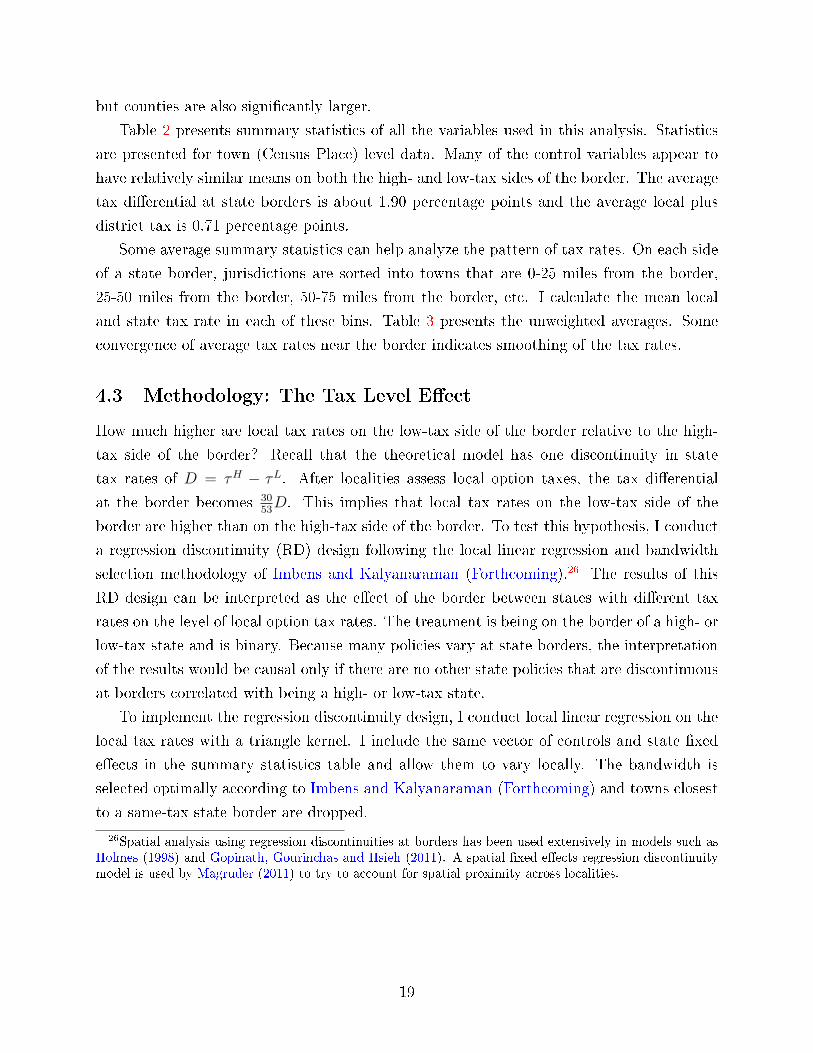
but counties are also signi�cantly larger.

Table 2 presents summary statistics of all the variables used in this analysis. Statistics

are presented for town (Census Place) level data. Many of the control variables appear to

have relatively similar means on both the high- and low-tax sides of the border. The average

tax di�erential at state borders is about 1.90 percentage points and the average local plus

district tax is 0.71 percentage points.

Some average summary statistics can help analyze the pattern of tax rates. On each side

of a state border, jurisdictions are sorted into towns that are 0-25 miles from the border,

25-50 miles from the border, 50-75 miles from the border, etc. I calculate the mean local

and state tax rate in each of these bins. Table 3 presents the unweighted averages. Some

convergence of average tax rates near the border indicates smoothing of the tax rates.

4.3 Methodology: The Tax Level E�ect

How much higher are local tax rates on the low-tax side of the border relative to the high-

tax side of the border? Recall that the theoretical model has one discontinuity in state

tax rates of D = τH − τL. After localities assess local option taxes, the tax di�erential

at the border becomes 3053D. This implies that local tax rates on the low-tax side of the

border are higher than on the high-tax side of the border. To test this hypothesis, I conduct

a regression discontinuity (RD) design following the local linear regression and bandwidth

selection methodology of Imbens and Kalyanaraman (Forthcoming).26 The results of this

RD design can be interpreted as the e�ect of the border between states with di�erent tax

rates on the level of local option tax rates. The treatment is being on the border of a high- or

low-tax state and is binary. Because many policies vary at state borders, the interpretation

of the results would be causal only if there are no other state policies that are discontinuous

at borders correlated with being a high- or low-tax state.

To implement the regression discontinuity design, I conduct local linear regression on the

local tax rates with a triangle kernel. I include the same vector of controls and state �xed

e�ects in the summary statistics table and allow them to vary locally. The bandwidth is

selected optimally according to Imbens and Kalyanaraman (Forthcoming) and towns closest

to a same-tax state border are dropped.

26Spatial analysis using regression discontinuities at borders has been used extensively in models such asHolmes (1998) and Gopinath, Gourinchas and Hsieh (2011). A spatial �xed e�ects regression discontinuitymodel is used by Magruder (2011) to try to account for spatial proximity across localities.

19

4.4 Result: Are Local Taxes Higher on One Side of the Border?

Figure 7 graphically presents the results of the regression discontinuity design without con-

trols. Table 4 shows the regression results for various speci�cations. Speci�cations 1, 2,

3 and 4 present the results for local, local and district, county, and total local rates at the

state border. Speci�cation 4 is most preferred; it demonstrates how much the tax di�erential

at state borders falls after all local option taxes are assessed. Keeping in mind that many

things change at state borders, columns 5 and 6 present the results at county borders that

are not also state borders. Columns �ve and six are more likely to represent a causal e�ect,

given that fewer policies vary discontinuously at county borders than at state borders.

Recall that the average tax di�erential at state borders is about 1.90 percentage points.

The results from the RD design of the total local rate yield an estimate of -1.13: a town

(located precisely near the border) on the high-tax side assesses a local sales tax rate that

is 1.13 percentage points lower than an identical border town on the low-tax side. Thus,

the average tax di�erential falls from 1.90 percentage points to 0.87 percentage points. This

result is consistent with the theoretical prediction that local sales taxes reduce the state

tax di�erential approximately by one-half. The results for local plus district tax rates are

smaller, as expected, and imply that municipal taxes are about 0.352 percentage points lower

on the high-tax side. With regard to county borders, the results remain negative suggesting

that the discontinuity in county tax rates imply local taxes are higher on the low-tax side

of the county. The results at county borders are smaller because tax di�erentials at county

borders are much smaller than at state borders.

The RD results suggest that as the model developed in Section 3 predicts, local sales

taxes reduce tax di�erentials at state borders.

5 Estimating the Tax Gradient

The previous section has shown that local taxes are lower on the high-tax side of the border

than on the low-tax side of the border. What remains to be seen � and is the subject of this

section � is if this reduction occurs gradually with distance from the border.

5.1 Methodology: The Tax Gradient E�ect

My estimation strategy exploits the discontinuity in the state tax rates at borders to estimate

how local tax rates depend on distance from the border. I use a global polynomial regression

rather than the local linear regression above. A global polynomial regression is preferred to

local linear regression because the treatment will vary with the size of the discontinuity. It

20

is also preferred because I care about precisely estimating the marginal e�ects (the slope of

the tax gradient) conditional on the size of the di�erential and on distance.

I will allow distance to have a di�erent e�ect on local tax rates depending on the side of

the border on which a town is located because the theory implies the geographic pattern is

di�erent on the low- and high-tax sides of the borders. The �treatment� is de�ned as the size

of the di�erence in state tax rates at the border. As such, the state border will be allowed

to have a di�erent e�ect on local tax rates depending on the size of the notch at the border

and depending on a locality's distance.

Let l index localities, c index counties and s index states. Then, Xlc denotes observable

characteristics of locality l in county c. The matrix X includes variables from Census 2000

data at the Census Place level plus some other control variables generated using geographic

�les such as population, the median level of income, the fraction of the population with a

college education, the fraction of seniors, the fraction of residents working in another state

and county, the number of neighbors, town area and perimeter. To this matrix, I also add the

vote share received by Obama in the 2008 Presidential election in case political a�liations

determine a locality's choice of whether to use the sales tax, a dummy for proximity to

international borders, and a dummy for proximity to oceans or water.

The variable tlc will denote the local (town) plus sub-district tax rates.27 De�ne Rlc as

the di�erence between the state tax rate of the high-tax state and the state tax rate of the

low-tax state. For locality l, if the nearest neighbor is a relatively high-tax state, this will

be a positive number. If the neighbor is a relatively low-tax state, the di�erence will be

a negative number. Also, Hlc is a dummy variable that denotes whether locality l's state

is a high-tax state relative to the nearest neighboring state of jurisdiction l. And Slc is a

dummy variable that is equal to one when locality l's state has the same state tax rate as

its neighboring state.

De�ne the distance from a locality to the nearest state border as dlc and note it is always

positive, so that towns located �fty miles on either side of the border are identical with

respect to distance. The role that distance plays may be non-linear and di�er depending

on the side of the border.28 To do analysis on the tax gradient, I need to assume that

the relationship between d and local taxes is su�ciently �exible, and I allow it to be a

polynomial function of degree p. Denote this function in matrix form as G(dl), where each

27To proceed, I must assume that local tax rates are in equilibrium in my data. Given the large numberof observations that I have, this is a realistic assumption.

28Identifying the slope of the tax gradient will rely on a functional form dependent method. Lovenheim andSlemrod (2010) use dummy variables based on distance to obtain a �exible function of distance. Lovenheim(2008) and Harding, Leibtag and Lovenheim (Forthcoming) impose log(D) as the functional form becausethey do not have su�cient power to use a more �exible polynomial.

21

column represents a higher order term of the polynomial function∑p

k=1(dlc)k. Note that the

locality cannot manipulate dl, so that it cannot select whether it is on the high- or low-tax

side.

The reduced form equation designed to test whether the di�erence in state tax rates at

the border in�uences local tax rates has the following speci�cation:

tlc = β0 + β1Hlc + β2Slc + β3Rlc + β4RlcHlc +Xlcϕ+

G(dlc)ρ+RlcG(dlc)γ +HlcG(dlc)δ +RlcHlcG(dlc)α+

SlcG(dlc)θ + λTlc + ζs + εlc.

(5)

In expression 5, εl are unobservable characteristics that are speci�c to a locality. ζs are

state �xed e�ects and Tlc is the county tax rate for locality l. The variables γ, ρ, δ, α, and

θ are the vectors of coe�cients where each element of the vector denotes the coe�cient on

each term in the polynomial � linear, square, cubic, etc.

A standard RD would simply de�ne the treatment as Hlc, as done in in Section 4.3.

The above speci�cation allows the treatment to also vary by the size of the state tax rate

discontinuity Rlc and estimates separate distance functions for high-, low-, and same-tax

state borders. The coe�cient on G(dlc) will pick up the average e�ect of distance on local

tax rates � or put di�erently, the e�ect of distance from the border. The interaction of

the distance term with Rlc in RlcG(dl) allows the treatment to vary with the size of the

discontinuity. Because Rlc is negative for towns in relatively low-tax states and positive

for towns in relatively high-tax states, the treatment is di�erent on opposite sides of the

border, as the theory suggests. The interaction HlcG(dlc) will allow for the e�ect of being at

a particular distance from the border on the high-tax side to be di�erent than being at that

same distance on the low-tax side. The coe�cient on RlcHlcG(dlc) allows for the treatment

e�ect to vary depending on the side of the border. Lastly, SlcG(dlc) allows the estimated

distance function to be di�erent for towns where the nearest border has the same state tax

rate on both sides. The term, β1Hlc+β2Slc+β3Rlc+β4RlcHlc, represents the intercept of the

polynomial function of distance. It captures the e�ect of the notch when d = 0 and allows

for the polynomial to have a di�erent intercept in relatively high- or low-tax states.

The inclusion of state �xed e�ects controls for commonalities occurring within a state but

not across borders and helps mitigate any geo-spatial correlation among towns in the same

state. With state �xed e�ects, identi�cation is coming from within state variation of local

tax rates. The state dummies will help to control for variation in policies and unobservables

that is constant within states, such as political climates or state business policies. Critically,

the inclusion of the state �xed e�ects will also control for the level of the state tax rate in

state s.

22

Finally, Equation 5 uses town tax rates as the left-side variable. However, towns are

embedded in counties, which are within states. While the state �xed e�ects control for

the level of the state tax rate, they do not control for the level of the county tax rate. I

cannot directly include the county tax rate, Tlc, on the right hand side because it is likely

selected simultaneously with local rates and therefore is endogenous. As a result, I instrument

for the county tax rate using a standard instrument in the tax competition literature � a

subset of the X's at the county level. The justi�cation of this set of instruments can be

found in Brueckner (2003). Brülhart and Jametti (2006) apply the instrument to higher

levels of government as well. Instead of using the entire subset of the X's as instruments,

I will only use geographic variables (which are not often controls in previous studies) as

instruments because demographic variables are likely to be endogenous at the municipal

level. Particularly, I use the county area, county perimeter, and county number of neighbors

as instruments.

To justify these instruments, recall that the regression equation controls for town area,

town perimeter, and the number of neighbors for the town. Then, the exclusion restriction

requires that the instrument should have no partial e�ect on local taxes after controlling for

these variables. The direct impact of the number of neighbors, area and perimeter of the

county on local taxes is likely to be zero. County neighbors, area and perimeter a�ect the

county's tax rates, but will have no direct impact on the locality's tax rate so long as there

are multiple jurisdictions within a county and so long as counties are su�ciently large in size.

County borders were likely to be historically drawn on latitudes and longitudes or broader

geographic features. The number of neighbors, area, and perimeter depend on a county's

characteristics such as whether along a body of water, broader geographic features, and how

counties were divided historically. Because area and perimeter are historically drawn, the

evolution of time with these variables helps to make them exogenous. As a contrary point,

the town's area, number of neighbors and perimeter often depend on how municipalities were

historically formed within the county and the characteristics within the county when the town

borders were historically drawn � which in most cases were not at the same time county lines

were delineated.29 Furthermore, as an alternative to the instrumental variable approach, I

present additional results where the dependent variable in the estimating equation is equal

to the town plus county tax rate. Because county rates are now part of the variable of

interest in these speci�cations, I avoid having to instrument for the county tax rate and can

instead look for a gradient in the total e�ective tax rate. The sign and signi�cance of the tax

29I conduct a Hansen J test of over-identi�cation. The result of this test � J = 2.28 (p = .32), a failureto reject the null hypothesis that all the instruments are uncorrelated with the error � is suggestive that inthe presence of one valid instrument, the other instrument is also valid.

23

gradient remain the same.30 The F-statistic for instrument strength from the �rst stage is

30.20 (p = .00). I can now proceed using the regression analysis in Equation (5) to estimate

the e�ect within a state.

The coe�cients within γ , ρ, δ, and α are not informative as stand-alone parameters

because the marginal e�ect of distance is a non-linear function of dlc. In the case of a p order

polynomial, the marginal e�ects of distance on the local tax rate for the high-, low-, and

same-tax side of the border are given by Equation 6:

∂tlc∂dlc

≡ G′(dl) =

∑p

k=1 k[ρk + δk + (γk + αk)Rlc](dlc)k−1 forHlc = 1 &Slc = 0∑p

k=1 k[ρk + γkRlc](dlc)k−1 forHlc = 0 &Slc = 0∑p

k=1 k[ρk + θk](dlc)k−1 forHlc = 0 &Slc = 1,

(6)

where the coe�cients indexed by k indicate the coe�cient on the kth order term of the

polynomial.

From this expression, I can calculate the mean marginal e�ect (or mean derivative) of

distance on tax rates by calculating the sample mean of the estimated derivative conditional

on being in a high-, low-, or same-tax state relative to the neighbor. Letting Nb denote

the number of observations on a particular side of a border, the mean marginal e�ects

represent the slope of the tax gradient away from the discontinuity after averaging across

the conditional sample:

E

[∂tlc∂dlc

]=

1

Nb

Nb∑l=1

G′(dl). (7)

The mean derivative of the full sample is of little interest given that the theory indicates

it will be of opposite sign on di�erent sides of the border. Therefore, the summation in

Equation 7 is separately taken over all towns on the high-tax side, low-tax side, and same-

tax sides of the border and Nb adjusts appropriately. Standard errors for mean derivatives

are calculated using the Delta Method. I also calculate, but do not report, the marginal

e�ect evaluated at the mean, or G′(dlc). The derivative evaluated at the mean is biased

and inconsistent because of non-linearity in the derivative. The marginal e�ect given by

Equation (7) is a consistent estimate of the mean derivative in the conditional population

and is the preferred e�ect.

If the mean marginal e�ect is positive, tax rates are increasing as the distance from the

nearest border increases. If the e�ect is negative, then towns further from the border are

30The results of these regressions are available in an online appendix at http://www-personal.umich.edu/~dagrawal/research.htm. This is not, however, the preferred speci�cation because it will leave meunable to compare the tax gradient at state borders to the tax gradient at county borders � where the leftside variable must be the local tax rate.

24

setting lower tax rates than those at the border. In general, because the marginal e�ect

need not be identical for all values of dlc or Rlc, I will also report the mean marginal e�ects

evaluated at di�erent possible values of dlc and Rlc. The theory predicts that the mean

marginal e�ect on the high-tax side of the border will be positive and on the low-tax side of

the border will be negative. When state tax rates are the same, no e�ect should be evident.

The polynomial order is selected using �leave-one-out� cross-validation.31 The implied

root mean squared error from leave-one-out cross-validation is decreasing in the order of

the polynomial until it reaches a minimum of .6625 at a polynomial order of �ve; thus, the

quintic polynomial is the preferred speci�cation. In addition, I ocularly compare the �t of the

predicted values from a global polynomial regression to the calculations using the local linear

regression described above. Figure 8 compares the �t of a quintic polynomial to the results

of the local linear regression. The quintic polynomial �ts the local linear regression almost

identically � both with respect to the curvature and the levels of the tax rates. Conducting

the same comparison for lower degree polynomials is less accurate.

5.2 Results: How Steep Is the Tax Gradient?

Table 5 presents the full set of coe�cients on several speci�cations of Equation 5 along

with the mean derivatives associated with them, scaled to represent a 100 mile change.

Speci�cation 1 includes only a quintic polynomial in distance. Column 2 adds local controls

and column 3 adds state �xed e�ects. Column 4 instruments for the county tax rate, which

is the preferred speci�cation.

The coe�cients on some control variables are worth highlighting. Having a higher fraction

of people who work in-county and in-state implies the tax base is less mobile across state

lines, and results in higher local tax rates. Higher income jurisdictions have lower tax rates,

suggesting that they may be more able to use the property tax as an alternative revenue

source. Towns near oceans have higher tax rates, consistent with a model located along

a line-segment where the jurisdictions at the end of the line set higher rates. On average,

jurisdictions near international borders set lower tax rates even though the international

borders are all high-tax borders. This suggests that towns near the international border see

no gain to exporting the tax to foreign consumers by raising the rates, but do not view the

border as closed. The number of neighbors has a positive sign. Finally, the coe�cient on

the instrumented county tax rate is negative and signi�cant � suggesting that higher county

31The process of cross-validation estimates equation 5, omitting one observation from the data set. Theprocess is repeated 16,781 times, omitting each observation from the data set once and calculating the rootmean squared error each time. I then calculate the average root mean squared error for all the omittedobservations. After repeating the cross-validation techniques for polynomials up to an order of eight, I selectthe polynomial that yields the smallest average root mean squared error.

25

taxes reduce local sales taxes.32

In the preferred speci�cation, the mean derivative on the low-tax side of the state border

is signi�cant and of the expected sign: -0.102. Thus, moving a town 100 miles away from

its high-tax state neighbor � assuming constant marginal e�ects � will decrease its local tax

rate by just over one tenth of a percentage point. Alternatively said, a one mile change has

a -.102 basis point change on local rates. Interpreting this in the context of the average local

tax rate, which is approximately 0.71 percent, implies that average local taxes are about

15% lower 100 miles away from the border. The gradient for towns with a same-tax state

neighbor is insigni�cant. For a town on the high-tax side of the border, the marginal e�ects

are slightly larger in absolute value (-.197) but are unexpectedly negative.

How robust are the results to reasonable alternative speci�cations? With regard to the

marginal e�ects, Table 6 presents the marginal e�ects for a variety of speci�cations, with

column 1 denoting the baseline results. In general, signi�cantly negative results on the

low-tax and high-tax side of the border are found. One speci�cation eliminates towns near

international borders, in case these borders are e�ectively closed to purchases. Another

speci�cation eliminates towns that are most proximate to the ocean.33 One reason for doing

this is that if the theoretical model were on a line segment instead of a circle, towns at the

end of the line segment have incentive to raise their tax rates because they only have one

neighbor. Column 3 indicates international borders may be di�erent than state borders.

Because the gradient becomes slightly steeper when excluding these jurisdictions (always

located on the low-tax side), it suggests that towns near international borders are less likely

to be able to charge a mark-up over their interior neighbors � perhaps because of di�erences

in the pre-tax price. Column 4 also seems to indicate that the towns near the ocean set

higher rates than their interior neighbors in low-tax states. Because the gradient becomes

steeper when excluding these towns, this suggests that towns near the ocean and away from

the border are setting higher rates than border towns, which is consistent with a Hotelling

style model where towns at the end of the line segment set higher rates.

Speci�cation 5 allows the reader to determine the marginal e�ect in hours instead of

miles. The marginal e�ects with a quintic in driving time indicates that a one-hour drive

from the border lowers tax rates .06 percentage points on the low side and by .10 percentage

points on the high side. Comparing this to speci�cation 1 indicates that the marginal e�ect

of driving 100 miles is approximately equal to the marginal e�ect of a driving time of two

hours. Columns 7 and 8 are important to decompose the results when neighboring states do

32Such a �nding � the relative magnitude of the vertical and horizontal externalities in the presence ofmultiple federations (counties) � is interesting in its own right, and is the subject of Agrawal (2011b).

33As an alternative, I interact the dummy variables for proximity to international borders and water withthe distance functions and �nd similar results.

26

not assess local option sales taxes (LOST). Recall that 16 states do not allow LOST. It may

be expected that the nature of the competition at these borders is di�erent than at a border

where both states allow LOST. When the neighbor does not allow LOST, the slope of the

gradient becomes much steeper on the low-tax side. Additionally, on the high-tax side, the

slope of the gradient becomes positive � and matches the predicted results of the theory.

This suggests that not having a local competitor on the opposite side of the border makes it

more likely that localities will reduce discontinuities in state tax rates. In addition to those

particular extensions, the decreasing tax gradient for low-tax states is highly robust.34

Table 7 shows that the results are robust to the order of the polynomial (columns 2 and

3). Columns 4 and 5 suggest that giving all states equal weight in the data and weighting

by population preserves the expected results. The results weighted by population increase

the steepness of the slope dramatically, suggesting that high population jurisdictions may

be more likely to be located near the border, where the gradient is steepest. Speci�cation 6

interacts all the state �xed e�ects and all the control variables with a polynomial in distance

and allows the coe�cients on these interactions to vary on the high-, low- and same-tax

side of the border. Such a speci�cation removes any possibility of coincidental correlation

with the distance function and allows each state to have its own tax gradient. The results

increase in magnitude and in signi�cance. Column 8 includes state �xed e�ects and state-

border-pair �xed e�ects, such that all the identifying variation comes from variation in local

taxes within only one border region in a state. Such a speci�cation controls for the level of

all state controls and controls for the possibility that the east border of a state may be very

di�erent from the west border (i.e., the presence of mountains or rivers, etc.). The last three

columns of Table 7 restrict the sample to towns within 150, 98, and 40 miles of the border.

The restriction of 98 miles is the optimal bandwidth of the local linear regressions above. In

these speci�cations I re-select the order of the polynomial for each restricted sample by the

cross-validation method above. Notice when the sample is restricted to a local region around

the border, the tax gradient becomes steepest and the gradient on the high-tax side becomes

insigni�cant. From Table 7, it can be seen that as the estimating area becomes larger, the

steepness of the tax gradient becomes smaller. This suggests that the mean derivatives are

strongest in a local region of the border � where cross-border shopping is likely to be most

salient.

Many of the coe�cients for the high- and low-tax side are similar in magnitude and sign.

Because of the similar estimates on both sides of the border, I must consider the possibility

34Column 2 indicates the results are robust to a binary treatment. The results are also robust to excludingsome states where local taxes are not extensively utilized (column 6), to using local taxes only as thedependent variable (column 9), and to using county plus local plus district taxes as the dependent variable,thus avoiding the need to instrument for county tax rates (column 10).

27

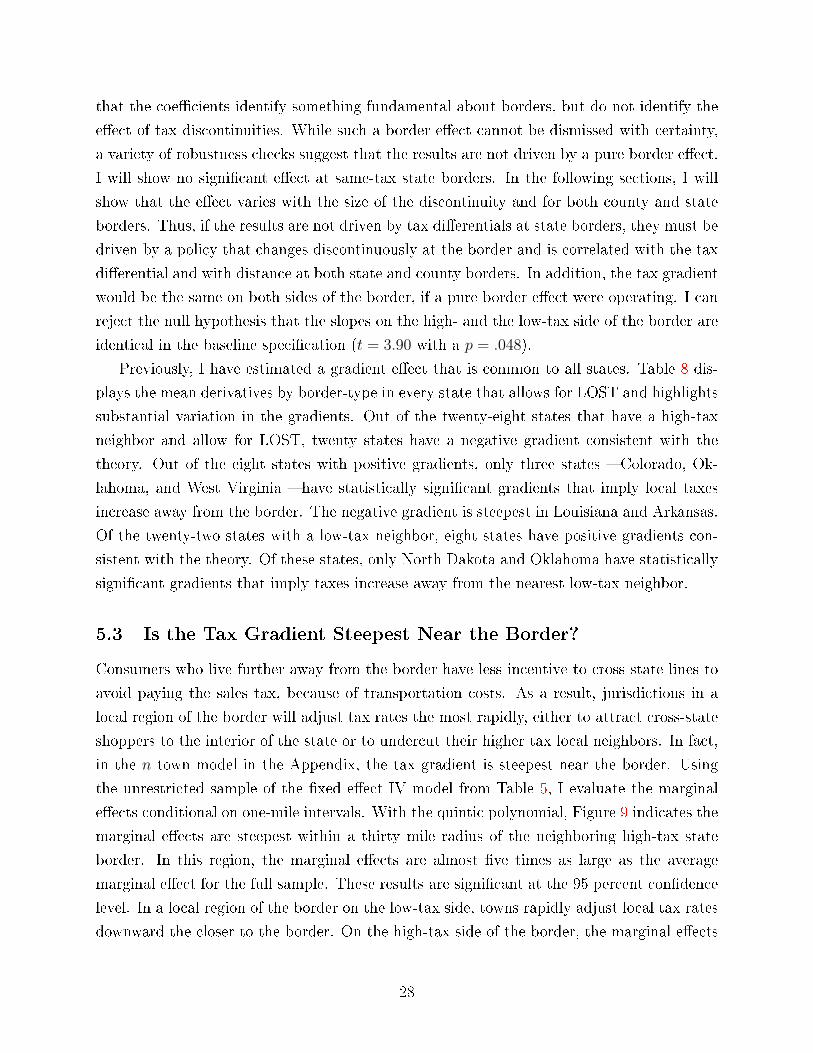
that the coe�cients identify something fundamental about borders, but do not identify the

e�ect of tax discontinuities. While such a border e�ect cannot be dismissed with certainty,

a variety of robustness checks suggest that the results are not driven by a pure border e�ect.

I will show no signi�cant e�ect at same-tax state borders. In the following sections, I will

show that the e�ect varies with the size of the discontinuity and for both county and state

borders. Thus, if the results are not driven by tax di�erentials at state borders, they must be

driven by a policy that changes discontinuously at the border and is correlated with the tax

di�erential and with distance at both state and county borders. In addition, the tax gradient

would be the same on both sides of the border, if a pure border e�ect were operating. I can

reject the null hypothesis that the slopes on the high- and the low-tax side of the border are

identical in the baseline speci�cation (t = 3.90 with a p = .048).

Previously, I have estimated a gradient e�ect that is common to all states. Table 8 dis-

plays the mean derivatives by border-type in every state that allows for LOST and highlights

substantial variation in the gradients. Out of the twenty-eight states that have a high-tax

neighbor and allow for LOST, twenty states have a negative gradient consistent with the

theory. Out of the eight states with positive gradients, only three states � Colorado, Ok-

lahoma, and West Virginia � have statistically signi�cant gradients that imply local taxes

increase away from the border. The negative gradient is steepest in Louisiana and Arkansas.

Of the twenty-two states with a low-tax neighbor, eight states have positive gradients con-

sistent with the theory. Of these states, only North Dakota and Oklahoma have statistically

signi�cant gradients that imply taxes increase away from the nearest low-tax neighbor.

5.3 Is the Tax Gradient Steepest Near the Border?

Consumers who live further away from the border have less incentive to cross state lines to

avoid paying the sales tax, because of transportation costs. As a result, jurisdictions in a

local region of the border will adjust tax rates the most rapidly, either to attract cross-state

shoppers to the interior of the state or to undercut their higher tax local neighbors. In fact,

in the n town model in the Appendix, the tax gradient is steepest near the border. Using

the unrestricted sample of the �xed e�ect IV model from Table 5, I evaluate the marginal

e�ects conditional on one-mile intervals. With the quintic polynomial, Figure 9 indicates the

marginal e�ects are steepest within a thirty mile radius of the neighboring high-tax state

border. In this region, the marginal e�ects are almost �ve times as large as the average

marginal e�ect for the full sample. These results are signi�cant at the 95 percent con�dence

level. In a local region of the border on the low-tax side, towns rapidly adjust local tax rates

downward the closer to the border. On the high-tax side of the border, the marginal e�ects

28

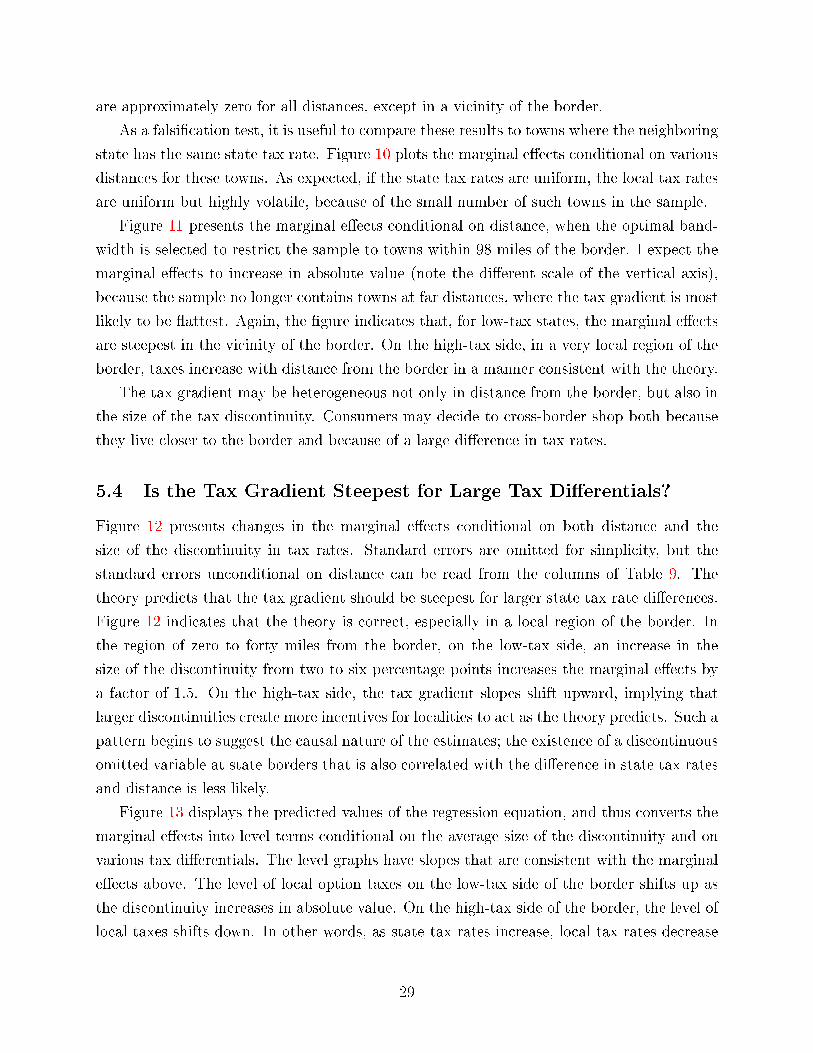
are approximately zero for all distances, except in a vicinity of the border.

As a falsi�cation test, it is useful to compare these results to towns where the neighboring

state has the same state tax rate. Figure 10 plots the marginal e�ects conditional on various

distances for these towns. As expected, if the state tax rates are uniform, the local tax rates

are uniform but highly volatile, because of the small number of such towns in the sample.

Figure 11 presents the marginal e�ects conditional on distance, when the optimal band-

width is selected to restrict the sample to towns within 98 miles of the border. I expect the

marginal e�ects to increase in absolute value (note the di�erent scale of the vertical axis),

because the sample no longer contains towns at far distances, where the tax gradient is most

likely to be �attest. Again, the �gure indicates that, for low-tax states, the marginal e�ects

are steepest in the vicinity of the border. On the high-tax side, in a very local region of the

border, taxes increase with distance from the border in a manner consistent with the theory.

The tax gradient may be heterogeneous not only in distance from the border, but also in

the size of the tax discontinuity. Consumers may decide to cross-border shop both because

they live closer to the border and because of a large di�erence in tax rates.

5.4 Is the Tax Gradient Steepest for Large Tax Di�erentials?

Figure 12 presents changes in the marginal e�ects conditional on both distance and the

size of the discontinuity in tax rates. Standard errors are omitted for simplicity, but the

standard errors unconditional on distance can be read from the columns of Table 9. The

theory predicts that the tax gradient should be steepest for larger state tax rate di�erences.

Figure 12 indicates that the theory is correct, especially in a local region of the border. In

the region of zero to forty miles from the border, on the low-tax side, an increase in the

size of the discontinuity from two to six percentage points increases the marginal e�ects by

a factor of 1.5. On the high-tax side, the tax gradient slopes shift upward, implying that

larger discontinuities create more incentives for localities to act as the theory predicts. Such a

pattern begins to suggest the causal nature of the estimates; the existence of a discontinuous

omitted variable at state borders that is also correlated with the di�erence in state tax rates

and distance is less likely.

Figure 13 displays the predicted values of the regression equation, and thus converts the

marginal e�ects into level terms conditional on the average size of the discontinuity and on

various tax di�erentials. The level graphs have slopes that are consistent with the marginal

e�ects above. The level of local option taxes on the low-tax side of the border shifts up as

the discontinuity increases in absolute value. On the high-tax side of the border, the level of

local taxes shifts down. In other words, as state tax rates increase, local tax rates decrease

29

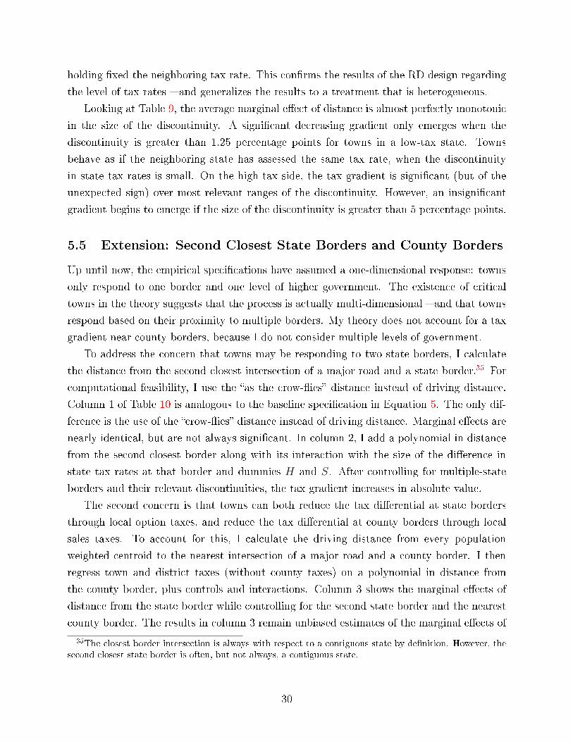
holding �xed the neighboring tax rate. This con�rms the results of the RD design regarding

the level of tax rates � and generalizes the results to a treatment that is heterogeneous.

Looking at Table 9, the average marginal e�ect of distance is almost perfectly monotonic

in the size of the discontinuity. A signi�cant decreasing gradient only emerges when the

discontinuity is greater than 1.25 percentage points for towns in a low-tax state. Towns

behave as if the neighboring state has assessed the same tax rate, when the discontinuity

in state tax rates is small. On the high-tax side, the tax gradient is signi�cant (but of the

unexpected sign) over most relevant ranges of the discontinuity. However, an insigni�cant

gradient begins to emerge if the size of the discontinuity is greater than 5 percentage points.

5.5 Extension: Second Closest State Borders and County Borders

Up until now, the empirical speci�cations have assumed a one-dimensional response: towns

only respond to one border and one level of higher government. The existence of critical

towns in the theory suggests that the process is actually multi-dimensional � and that towns

respond based on their proximity to multiple borders. My theory does not account for a tax

gradient near county borders, because I do not consider multiple levels of government.

To address the concern that towns may be responding to two state borders, I calculate

the distance from the second closest intersection of a major road and a state border.35 For

computational feasibility, I use the �as the crow-�ies� distance instead of driving distance.

Column 1 of Table 10 is analogous to the baseline speci�cation in Equation 5. The only dif-

ference is the use of the �crow-�ies� distance instead of driving distance. Marginal e�ects are

nearly identical, but are not always signi�cant. In column 2, I add a polynomial in distance

from the second closest border along with its interaction with the size of the di�erence in

state tax rates at that border and dummies H and S. After controlling for multiple-state

borders and their relevant discontinuities, the tax gradient increases in absolute value.

The second concern is that towns can both reduce the tax di�erential at state borders

through local option taxes, and reduce the tax di�erential at county borders through local

sales taxes. To account for this, I calculate the driving distance from every population

weighted centroid to the nearest intersection of a major road and a county border. I then

regress town and district taxes (without county taxes) on a polynomial in distance from

the county border, plus controls and interactions. Column 3 shows the marginal e�ects of

distance from the state border while controlling for the second state border and the nearest

county border. The results in column 3 remain unbiased estimates of the marginal e�ects of

35The closest border intersection is always with respect to a contiguous state by de�nition. However, thesecond closest state border is often, but not always, a contiguous state.

30

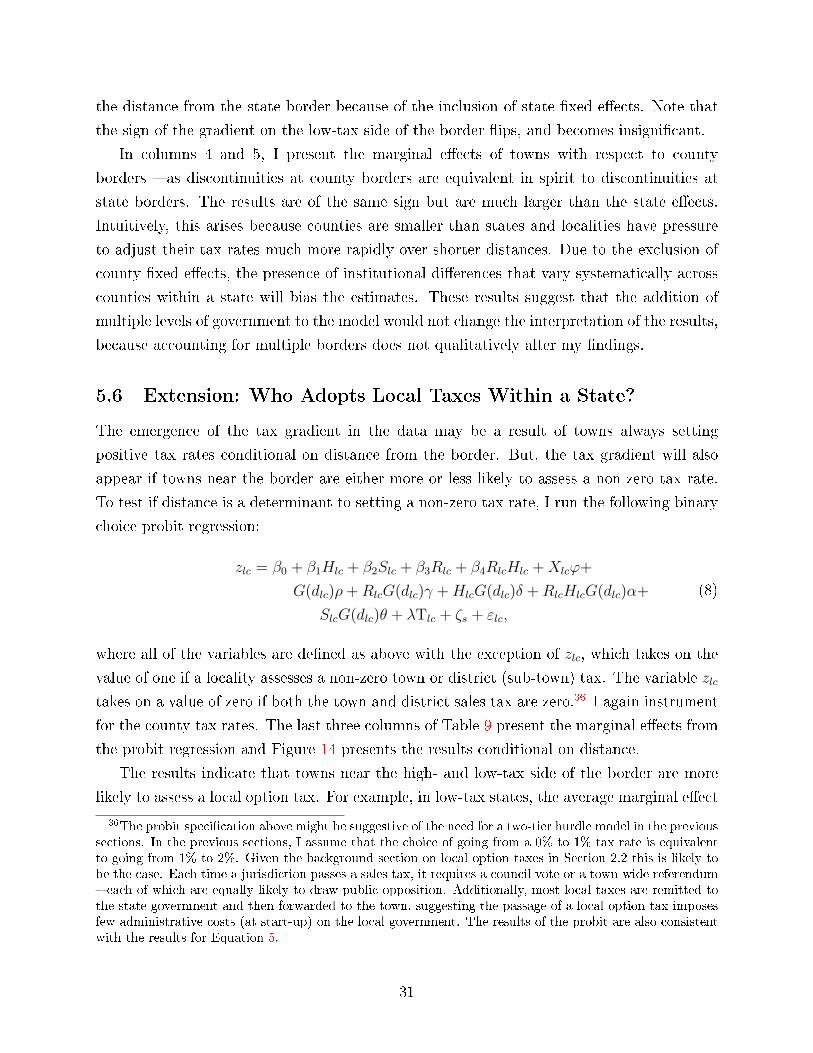
the distance from the state border because of the inclusion of state �xed e�ects. Note that

the sign of the gradient on the low-tax side of the border �ips, and becomes insigni�cant.

In columns 4 and 5, I present the marginal e�ects of towns with respect to county

borders � as discontinuities at county borders are equivalent in spirit to discontinuities at

state borders. The results are of the same sign but are much larger than the state e�ects.

Intuitively, this arises because counties are smaller than states and localities have pressure

to adjust their tax rates much more rapidly over shorter distances. Due to the exclusion of

county �xed e�ects, the presence of institutional di�erences that vary systematically across

counties within a state will bias the estimates. These results suggest that the addition of

multiple levels of government to the model would not change the interpretation of the results,

because accounting for multiple borders does not qualitatively alter my �ndings.

5.6 Extension: Who Adopts Local Taxes Within a State?

The emergence of the tax gradient in the data may be a result of towns always setting

positive tax rates conditional on distance from the border. But, the tax gradient will also

appear if towns near the border are either more or less likely to assess a non-zero tax rate.

To test if distance is a determinant to setting a non-zero tax rate, I run the following binary

choice probit regression:

zlc = β0 + β1Hlc + β2Slc + β3Rlc + β4RlcHlc +Xlcϕ+

G(dlc)ρ+RlcG(dlc)γ +HlcG(dlc)δ +RlcHlcG(dlc)α+

SlcG(dlc)θ + λTlc + ζs + εlc,

(8)

where all of the variables are de�ned as above with the exception of zlc, which takes on the

value of one if a locality assesses a non-zero town or district (sub-town) tax. The variable zlc

takes on a value of zero if both the town and district sales tax are zero.36 I again instrument

for the county tax rates. The last three columns of Table 9 present the marginal e�ects from

the probit regression and Figure 14 presents the results conditional on distance.

The results indicate that towns near the high- and low-tax side of the border are more

likely to assess a local option tax. For example, in low-tax states, the average marginal e�ect

36The probit speci�cation above might be suggestive of the need for a two-tier hurdle model in the previoussections. In the previous sections, I assume that the choice of going from a 0% to 1% tax rate is equivalentto going from 1% to 2%. Given the background section on local option taxes in Section 2.2 this is likely tobe the case. Each time a jurisdiction passes a sales tax, it requires a council vote or a town-wide referendum� each of which are equally likely to draw public opposition. Additionally, most local taxes are remitted tothe state government and then forwarded to the town, suggesting the passage of a local option tax imposesfew administrative costs (at start-up) on the local government. The results of the probit are also consistentwith the results for Equation 5.

31

is -0.47. If this e�ect were constant, a town 100 miles from the border is 47 percent less likely

to have a local option tax compared to an identical town on the border. For the high-tax

state, the e�ect is 44 percent. The negative e�ect on the low-tax side is consistent with the

tax gradient decreasing away from the border. Towns near the border realize they can export

some of the town's tax burden to residents of the neighboring state and substitute to a local

option sales tax � perhaps as a mechanism to reduce the property tax. On the high-tax side,

towns near the border are more likely to have local option taxes as well, which is inconsistent

with the theory and may explain why no tax gradient emerges in the tax rates. However, as

the size of the discontinuity increases, the marginal e�ect on the probability of assessing a

local option tax is decreasing.

5.7 Discussion

In summary, in a local region of the border, towns in low-tax states keep their local tax

rates relatively high in order to export a large fraction of their tax burden to cross-border

shoppers. This is especially salient when the size of the tax gap is largest � and when the

town is most likely to attract cross-border shoppers who will bear some of the burden of

the tax. As towns get further from the border, tax rates fall, and they fall the fastest the

closest to the border � suggesting that towns undercut their neighbor in an e�ort to attract

cross-border shoppers. However, towns farther away from the border need a much lower tax

rate to attract residents from the low-tax state or from the border towns in their state. The

empirical evidence here suggests that for towns beyond �fty miles from the border, tax rates

are relatively constant with respect to distance and even slightly increasing.

On the high-tax side, the results do not line up with the theory, except in the case of

very large state tax rate di�erences. An explanation for these e�ects is that the local tax

rates on the high-tax side are much lower on average. Localities on the high-tax side of

the border may not be constrained when assessing local option taxes because they do not

anticipate further cross-border shopping problems. If the state tax rate is high, localities

may anticipate that any remaining consumers have a low elasticity � leading the jurisdiction

to raise the rate without fear of losing shoppers. An alternative explanation is suggested by

Harding, Leibtag and Lovenheim (Forthcoming) who �nd that the incidence of the tax varies

with distance from neighboring low-tax states. If �rms near the border pass on less of the

tax to consumers, the �rms may be already smoothing the post-tax price in the same manner

the localities would. If towns know that �rms near the border bear more of the burden of

the tax, the jurisdiction will have incentives to raise taxes near the border. These authors

�nd no evidence that the incidence varies with distance on the low-tax side of borders. If

32

incidence e�ects do not vary with distance in low-tax states, then the towns will adjust the

local tax rate as a function of distance because the local government cannot rely on �rms

to vary the incidence of the tax with distance. A �nal explanation is yardstick competition

by municipalities. If jurisdictions engage in yardstick competition, governments observe the

tax rate levels of nearby jurisdictions and mimic the tax rate. For border localities on the

high-tax side of the border, some of the local neighbors are on the low-tax side of the border.

Because these neighbors in the low-tax state set relatively high tax rates, border jurisdictions

on the high-tax side may look to their neighbors in the opposing state and set a relatively

high tax rate compared to a town interior to their state.

The level of local tax rates is substantially higher for border towns on the low-tax side of

the border. And the existence of an economically and statistically signi�cant tax gradient

implies that discontinuities at state borders continue to a�ect the elasticity of demand in

local jurisdictions away from the border by inducing a unique form of tax competition where

jurisdictions account for this discontinuity.

6 Conclusion

Identical local governments within a state will have incentives to di�erentiate their taxes to

smooth the discontinuity in the total tax rate at the border, even when the state government

prefers a higher or lower state tax rate than its neighbors. Discontinuities at state borders

make identical jurisdictions heterogeneous based on the jurisdiction's location within a state

and its ability to attract cross-border shoppers.

The discontinuity in the tax system at state borders induces welfare distortions with

respect to consumption as some residents cross borders to purchase lower-tax goods. It is

also likely to create horizontal inequities � where individuals with the same ability to pay

actually pay di�erent taxes � if some residents cross-border shop while others do not. A

continuous tax system will reduce these welfare distortions, but will still have horizontal

inequities if some individuals purchase goods a few neighboring jurisdictions away.

Moreover, as in Kleven and Slemrod (2009), �tax-driven product innovations� will distort

the location of the �rm. Such innovations require no technological innovations, but distort the

characteristics of the goods � where the characteristic is the location of sale � to avoid taxes.

In the context of the retail sales tax, this innovation arises as �rms distort the locational

characteristics of the good to the tax favorable side of the border in order to capture cross-

border shoppers.37 Absent the tax di�erential, the �rm may have decided to locate on the

37The model presented in this paper did not allow for �rms to choose their location decisions. However,shopping patterns must be linked with retail locations.

33

other side of the border. Instead, the locational characteristics become ine�cient because

of the �rm's decision. I uncover a local tax gradient, which reduces these production and

consumption distortions at state borders.

Even if the �rst-best tax system � as set by a global welfare maximizer who is constrained

by varying state tax rates � is a perfectly continuous function of distance from the border, it

is likely that this system is administratively infeasible. However, as in the model presented

above, smoothing the size of the discontinuity through discrete steps in the tax system (that

are a function of distance) is likely to happen as a result of tax competition over local tax

rates � approximating a continuous policy. Although the discrete steps will induce additional

notches within the tax system, the reduction in the larger distortion across the state will

almost certainly be welfare improving. The new distortions at local borders are virtually

guaranteed in any tax system given the infeasibility of an in�nite number of di�erentiated

tax rates.

Whether the tax gradient is optimal from a state government's perspective or if it is

optimal for a state to allow localities to adopt LOST raise di�erent questions than the global

planner's decision. Agrawal (2011a) shows in a model where states maximize social welfare

that the optimal pattern for the state depends critically on the elasticity of cross-border

shopping, the inequality in consumption pro�les, and the relative magnitudes of the tax

base and exporting e�ects. If the elasticity of cross-border shopping is below a critical value,

then it is advantageous to have higher tax rates � as empirically found in this paper � in the

border region of a low-tax state. For it to be optimal to set higher rates in the border region

of a high-tax state, the within-state inequalities in consumption induced by cross-border

shopping must be su�ciently large such that the social planner would want to eliminate

these inequalities by raising the border region's rate. It may be welfare enhancing from the

state government's perspective to allow localities to assess local sales taxes.

This paper shows that federalism is a partial solution to the administrative di�culty of

centrally implementing a tax system where tax rates are a continuous function of distance

from the border. If local jurisdictions can set additional retail sales taxes, the salience

of the state border would directly in�uence localities close to that border. On the other

hand, jurisdictions located far from the border worry less about the notches because these

jurisdictions do not have in-�ows or out-�ows of cross-border shoppers.

Empirically, I show that conditional on a set of observables, distance is a signi�cant factor

in the pattern of local option taxes. Jurisdictions on the low-tax side of the border that are

relatively close to the border have higher tax rates than identical jurisdictions farther away

from the border. These jurisdictions have a smaller elasticity of demand and export the

tax burden to cross-border shoppers from the neighboring state. Although local tax rates

34

gradually o�set border di�erences on the low-tax side, the results have an unexpected sign

on the high-tax side. Identical towns on opposite sides of the border also di�er in the level

of local tax rates with local taxes substantially lower on the high-tax side of the border.

Although a discrete tax gradient is not the �rst-best outcome of a perfectly continuous tax

gradient, the empirical evidence suggests that local option taxes will gradually smooth tax

di�erentials over longer distances on the low-tax side.

The methodologies I develop in the paper are broadly applicable to analyzing how local

governments respond to any policies that vary discontinuously at a border. For example,

suppose states implement varying environmental restrictions on �rms. At the margin, �rms

may choose to relocate to the side of the border with lower emission standards. Localities

may adopt local regulations as a function of distance to the border in order to discourage

�rms from relocating and to reduce the regulatory di�erential at the border. More gen-

erally, �notched� or discontinuous policies are widespread and often are heterogeneous in

magnitude. The methodologies developed in this paper account for this heterogeneity. Re-

searchers can apply the theoretical and empirical methodologies introduced in this paper to

test if �notched� policies induce jurisdictions to implement policies that vary with distance

from the discontinuity.

7 Appendix

7.1 Proof of Uniqueness of the Equilibrium

In the paper, I derive conditions under which an equilibrium will exist. Existence follows from

concavity and continuity of the best response functions, plus certain additional conditions

outlined in the text. Once existence is shown, I prove below that any equilibrium in this

model will be unique for the case of a multiple state, n town model. The solution to a three

state model with n towns is characterized by the equation At = b. The proof generalizes to

a multi-state model simply by changing the dimensions of the vectors and the elements of

35

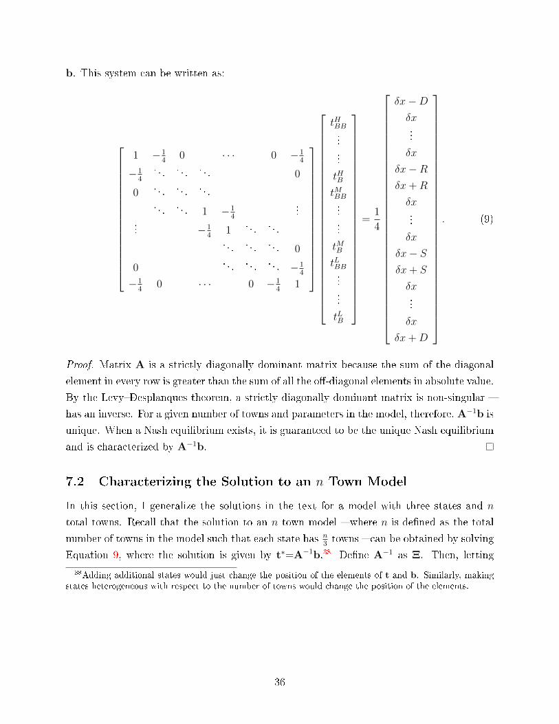
b. This system can be written as:

1 −14

0 · · · 0 −14

−14

. . . . . . . . . 0

0. . . . . . . . .. . . . . . 1 −1

4

...... −1

41

. . . . . .. . . . . . . . . 0

0. . . . . . . . . −1

4

−14

0 · · · 0 −14

1

tHBB......

tHBtMBB......

tMBtLBB......

tLB

=1

4

δx−Dδx...

δx

δx−Rδx+R

δx...

δx

δx− Sδx+ S

δx...

δx

δx+D

. (9)

Proof. Matrix A is a strictly diagonally dominant matrix because the sum of the diagonal

element in every row is greater than the sum of all the o�-diagonal elements in absolute value.

By the Levy�Desplanques theorem, a strictly diagonally dominant matrix is non-singular �

has an inverse. For a given number of towns and parameters in the model, therefore, A−1b is

unique. When a Nash equilibrium exists, it is guaranteed to be the unique Nash equilibrium

and is characterized by A−1b.

7.2 Characterizing the Solution to an n Town Model

In this section, I generalize the solutions in the text for a model with three states and n

total towns. Recall that the solution to an n town model � where n is de�ned as the total

number of towns in the model such that each state has n3towns � can be obtained by solving

Equation 9, where the solution is given by t∗=A−1b.38 De�ne A−1 as Ξ. Then, letting

38Adding additional states would just change the position of the elements of t and b. Similarly, makingstates heterogeneous with respect to the number of towns would change the position of the elements.

36

` = −14, the determinant of Ξ is given by:

det(Ξ) = 1 +

bn−12 c∑

k=1

(−1)kn(n− k − 1)!`2k

(n− 2k)!k!+ 2`n1(n is odd)− 4`n1(n is even&

n

2is odd),

(10)

where 1(•) is an indicator function that takes on the value one if • is true and takes on the

value zero otherwise. Then, I can decompose Ξ such that Ξ = 1

det(Ξ)Ψ . Letting i index

rows (the town) and j index columns (the town's neighbors' positions on the circle), the

elements of Ψ are given by ψi,j. If n is even, the elements of the �rst row in Ψ can be solved

for as:

ψ1,j =

φj

−2`φn2

φ2+n−j

for j = 1, ..., n2

for j = n2

+ 1

for j = n2

+ 2, ..., n,

(11)

while if n is odd, the elements are given by:

ψ1,j =

φj

φj + ξj

φ2+n−j + ξ2+n−j

for j = 1

for j = 2, ..., n−12

+ 1

for j = n−12

+ 2, ..., n,

(12)

where

φj =

bn−j2 c∑k=0

(−1)k(n− j − k)!`2k+j−1

(n− j − 2k)!k!, (13)

and

ξj =

b j−22 c∑

k=0

(−1)j+k−2(j − 2 + k)!`n−j+2k−1

(j − 2)!k!. (14)

Note that as they are written above, equations 11 and 13 only yield the elements of the

matrix's �rst row. Each of the subsequent rows will shift the elements of the previous row

one place over, where the �nal element of the row will become the �rst element of the row.

Therefore, for i > 1:

ψi,j = ψ1,r where r ≡ (j + n− r + 1)(modn), (15)

and (j + n− r + 1)(modn) = j + n− r + 1− n⌊j+n−r+1

n

⌋.

The equilibrium tax rates can now be characterized as t∗=A−1b = Ξb = 1

det(Ξ)Ψb. It

37

should be noted thatn∑j=1

(−`)δxψi,j =1

2δx ∀i. (16)

To complete the characterization of the solution, one must determine how the size of the

discontinuities in b that multiply the inverted matrix enter the solution. Under the as-

sumption that all states are uniform in size, the discontinuities D,R, andS will additively

enter into town i's equilibrium tax rates as (−`)(ψi,n − ψi,1)D, (−`)(ψi,n3

+1 − ψi,n3)R, and

(−`)(ψi, 2n3

+1 − ψi, 2n3

)S. Recalling that D = R + S because of the circular setup of the

problem, if x > x∗, the equilibrium tax rates can be characterized as:

t∗i =1

2δx−

`(ψi,n − ψi,1 + ψi,n3

+1 − ψi,n3)R + `(ψi,n − ψi,1 + ψi, 2n

3+1 − ψi, 2n

3)S

det(Ξ)∀i. (17)

Notice that if the states were asymmetric with respect to the number of towns, the above

expressions could be modi�ed by picking the jth element of Ψ appropriately � where the

number of towns are adjusted on the j index of ψ.

7.3 Methodology for Calculating Distance from the Border

In this section, I outline the methodology for calculating distance from the border. Arc-GIS

is used to calculate this variable and all base map �les necessary to calculate distance from

the border are available on the Arc-GIS / ESRI map CD.39 Figure 15 shows the methodology

graphically.

I sometimes use the �as the crow-�ies� distance from the population weighted average

centroid of a place to the nearest intersection of a major road and a state border or foreign

country to calculate the distance from the border. The District of Columbia is counted

as a state, but Native American reservations are treated as localities. The justi�cation

for treating reservations as localities is that with some exceptions, purchases on Native

American reservations by non-tribal members are subject to state sales taxes. Furthermore,

reservations are often small and although they frequently sell cigarette purchases tax free,

they do not have extensive shopping outlets for many larger items. Many reservations have

also begun charging tribal tax rates on general sales.

To calculate distance from the border, I execute the following steps. When calculating

distance, the projection system utilized in the map �les is essential to guaranteeing that the

distance measure is accurate for all latitudes and longitudes. This requires that the projec-

39The section below utilizes jargon from mapping software, which may be unfamiliar to readers not familiarwith Arc-GIS.

38

tion system selected preserves distance attributes and that it be the same on all maps before

beginning any calculations. I select the North American Equidistant Conic Projection Sys-

tem. When the coordinate system is de�ned di�erently, I convert the coordinate system using

the NAD 1983 to WGS 1984 _ 1 geographic transformation option. This transformation

converts the coordinate system with an accuracy of plus or minus two meters.

First, in order to identify the tax rates at international crossings, I merge a detailed

polygon �le of the �fty states plus the District of Columbia with detailed �les of Canada and

Mexico. It is important to use a �detailed� �le that precisely traces out the border. Smoothed

�les may be o� several miles in many circumstances. I then convert the polygon �le into a

line �le that explicitly identi�es the geographic identi�cation number of the �left� and �right�

states. This identi�cation will allow me to record the neighboring state's tax rate. Second, I

overlay a detailed Census major roads �le. Census major roads are Class 1, 2, and 3 roads,

which include major highways and paved roads primarily used for transportation. These

classes of roads exclude dirt roads and primarily residential roads. Then, I �nd the precise

intersection of each state border line with a major road. This intersection is identi�ed with

a FID number, which can be used to identify the state border combination from the state

line �le. I drop all intersections that correspond to coastal areas or to major routes that are

de�ned as ferry crossings.

Third, I identify the population weighted centroid as the point in which the place would

balance on a scale if every person in that place were equal weight. To calculate this, I identify

the population distribution within a place using the population of every Census block in the

country.40 Let b index each Census block point given by population Pb and has latitude

φb and longitude λb. The population weighted center of place i is the latitude φ̄ and the

longitude λ̄ given by:

φ̄i = ΣPbφbΣPb

λ̄i =ΣPbλbCos(φb(

π180

))

ΣPbCos(φb(π

180)).

Fourth, I run a �near� command on the 25,000 population weighted centroids and the several

thousand intersections that I found above. This will calculate the nearest linear distance

from the intersection of the major roads and the state borders. Fifth, I conduct a spatial join

on the centroids with the level of geography I wish to analyze (call it a place polygon �le). I

de�ne a centroid as being within a place polygon if its point is contained entirely within the

polygon. This spatial join will attach the geographic identi�er of the Census place or county

to the centroid.

To calculate the second closest border crossing, I follow the method outlined above, but

40A Census block is the smallest unit of geography. In some cases, a block may be a large area with littleor no population. In other areas, a Census block may contain an entire apartment complex or building andmay have a population of several hundred.

39

instead of executing a near command in ArcGIS, I use the near table command. This will

calculate all of the nearest border crossings up to a particular threshold. I calculate 1000 of

the nearest border crossings for each place centroid. This is a su�cient number for me to

calculate the distance from the second closest border.

The data calculated above then can be merged based on geographic identi�cation numbers

to the Census data. However, the tax data does not contain geographic identi�ers, so I must

merge the data using name matching. In cases of merging by county, this is an easy process

and I am able to obtain a 99.9% match rate. One county does not match because it is not in

the tax data set. Census places are the closest to towns in the United States. Census places

contain no county information. In some states, Census places (and towns) cross county lines.

To deal with this issue, I intersect Census places and counties using a spatial join in ArcGIS.

This matches each place to a county that it overlaps. I can then name match Census places

to the tax data using place, county, and state names. Name matching to Census place data

obtains nearly a 90% match rate.41 I hand match any remaining observations.

Inevitably, a better measure of distance is actual driving distance. I calculate driving

distance using ArcGIS' network analyst toolbox. After following the �rst three steps above,

I use ESRI's street �le to calculate driving distance. The data in the street �le contains all

streets in the country, but note that the �nal destination I use will always be a major road

as above. I convert the data to a network data set so that it has street driving speeds within

it. To calculate driving distance, I locate the nearest minor street to a population weighted

centroid and to the major road crossings by searching within a �fty-mile radius. After doing

this, I need to specify how ArcGIS will calculate driving distance. Using the centroids as

origins and the border crossings as destinations, I use a time criterion to calculate distance

� that is I have GIS minimize the driving time to the nearest location.42

In addition, I need to make assumptions on how the individual drives to the border. I

assume that individuals follow a �hierarchical� method of driving � that is whenever possible,

I have ArcGIS route their travel via larger roads. I also require that individuals must

obey one-way streets or turn restrictions onto roads. However, I do not impose any other

restrictions � that is I do not restrict individuals from using alleys, four-wheel drive roads, or

ferry crossings.43 Using the network analyst, ArcGIS returns the driving distance (in miles)

and time (in minutes) for the shortest time path from each population weighted centroid to

the nearest intersection of a major road and state border.

41Recall some Census places are not towns and some towns are not Census places.42The alternative would be to use a distance criterion.43I impose these restrictions and �nd the driving distances are almost perfectly correlated.

40

7.4 Online Appendices

Online appendices are at http://www-personal.umich.edu/~dagrawal/research.htm and

contain two contributions. The �rst online appendix presents a very simple two-state model

of the tax gradient. The model is much simpler than the one in the text, but demonstrates

most of the intuition in a very stark manner. The second appendix presents all the �gures

and tables below for a regression speci�cation with the total local plus county tax rate as

the dependent variable. The results are very similar to the ones presented in the text.

References

Agrawal, David R. 2011a. �Games Within Borders: Are Geographically Di�erentiated

Taxes Optimal?� Working Paper, University of Michigan.

Agrawal, David R. 2011b. �Inter-federation Competition: Sales Tax Externalities with

Multiple Federations.� WorkingPaper, University of Michigan.

Brülhart, Marius, and Mario Jametti. 2006. �Vertical versus Horizontal Tax External-

ities: An Empirical Test.� Journal of Public Economics, 90: 2027�2062.

Brueckner, Jan K. 2003. �Strategic Interaction Among Governments: An Overview of

Empirical Studies.� International Regional Science Review, 26: 175�188.

Bucovetsky, Sam. 1991. �Asymmetric Tax Competition.� Journal of Urban Economics,

30(2): 167�181.

Fox, William F. 1986. �Tax Structure and the Location of Economic Activity Along State

Borders.� National Tax Journal, 39(4): 387�401.

Gopinath, Gita, Pierre-Olivier Gourinchas, and Chang-Tai Hsieh. 2011. �Interna-

tional Prices, Costs and Markup Di�erences.� American Economic Review, 101(6): 2450�

2486.

Harding, Matthew, Ephraim Leibtag, and Michael Lovenheim. Forthcoming. �The

Heterogeneous Geographic and Socioeconomic Incidence of Cigarette Taxes: Evidence

from Nielsen Homescan Data.� American Economic Journal: Economic Policy.

Hau�er, Andreas. 1996. �Tax Coordination with Di�erent Preferences for Public Goods:

Con�ict or Harmony of Interest.� International Tax and Public Finance, 3(1): 5�28.

41

Holmes, Thomas J. 1998. �The E�ect of State Policy on the Location of Manufacturing:

Evidence from State Borders.� Journal of Political Economy, 106(4): 667�705.

Hoyt, William. 2001. �Tax Policy Coordination, Vertical Externalities, and Optimal Taxa-

tion in a System of Hierarchical Governments.� Journal of Urban Economics, 50: 491�516.

Imbens, Guido, and Karthik Kalyanaraman. Forthcoming. �Optimal Bandwidth

Choice for the Regression Discontinuity Estimator.� Review of Economic Studies. Working

Paper, Harvard University.

Kanbur, Ravi, and Michael Keen. 1993. �Jeux Sans Frontières: Tax Competition and

Tax Coordination When Countries Di�er in Size.� American Economic Review, 83(4): 877�

892.

Kleven, Henrik Jacobsen, and Joel Slemrod. 2009. �A Characteristics Approach to

Optimal Taxation and Tax-Driven Product Innovation.� Working Paper, London School

of Economics and Political Science.

Lovenheim, Michael F. 2008. �How Far to the Border?: The Extent and Impact of Cross-

Border Casual Cigarette Smuggling.� National Tax Journal, 61(1): 7�33.

Lovenheim, Michael F., and Joel Slemrod. 2010. �Fatal Toll of Driving to Drink: The

E�ect of Minimum Legal Drinking Age Evasion on Tra�c Fatalities.� Journal of Health

Economics, 29(1): 62�77.

Luna, LeAnn. 2003. �Local Sales Tax Competition and the E�ect on County Governments'

Tax Rates and Tax Bases.� Journal of the American Taxation Association, 26(1): 43�67.

Luna, LeAnn, Donald J. Bruce, and Richard R. Hawkins. 2007. �Maxing Out: An

Analysis of Local Option Sales Tax Rate Increases.� National Tax Journal, 60(1): 45�63.

Magruder, Jeremy R. 2011. �High Unemployment Yet Few Small Firms: The Role of

Centralized Bargaining in South Africa.� Working Paper, University of California, Berke-

ley.

Merriman, David. 2010. �The Micro-geography of Tax Avoidance: Evidence from Littered

Cigarette Packs in Chicago.� American Economic Journal: Economic Policy, 2(2): 61�84.

Mikesell, John L. 1970. �Central Cities and Sales Tax Rate Di�erentials: The Border City

Problem.� National Tax Journal, 23(2): 206�213.

42

Mikesell, John L. 2010. �The Contribution of Local Sales and Income Taxes to Fiscal

Autonomy.� In Municipal Revenues and Land Policies. , ed. G. K. Ingram and Yu-Hung

Hong. Boston, MA:Lincoln Institute of Land Policy.

Nielsen, Søren Bo. 2001. �A Simple Model of Commodity Taxation and Cross-Border

Shopping.� Scandinavian Journal of Economics, 103(4): 599�623.

Research Institute of America. 2010. Guide to Sales and Use Taxes. New York,

NY:Thomson Publisher.

Sjoquist, David L., William Smith, Sally Wallace, and Mary Beth Walker. 2007.

�An Analysis of the Time to Adoption of Local Sales Taxes: A Duration Model Approach.�

Public Budgeting and Finance, 27(1): 20�40.

Slemrod, Joel. 2010. �Buenas Notches: Lines and Notches in Tax System Design.� Working

Paper, University of Michigan.

Tosun, Mehmet S., and Mark L. Skidmore. 2007. �Cross-Border Shopping and the Sales

Tax: An Examination of Food Purchases in West Virginia.� B.E. Journal of Economic

Analysis and Policy, 7(1): 1�18.

Trandel, Gregory. 1994. �Interstate Commodity Tax Di�erentials and the Distribution of

Residents.� Journal of Public Economics, 53(3): 435�457.

Walsh, Michael, and Jonathan Jones. 1988. �More Evidence on the Border Tax E�ect:

The Case of West Virginia, 1979-84.� National Tax Journal, 41(2): 261�265.

43

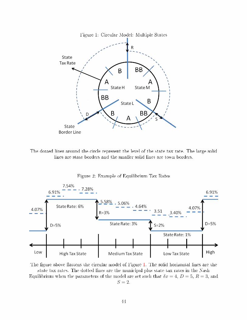
Figure 1: Circular Model: Multiple States

The dotted lines around the circle represent the level of the state tax rate. The large solidlines are state borders and the smaller solid lines are town borders.

Figure 2: Example of Equilibrium Tax Rates

The �gure above �attens the circular model of Figure 1. The solid horizontal lines are thestate tax rates. The dotted lines are the municipal plus state tax rates in the Nash

Equilibrium when the parameters of the model are set such that δx = 4, D = 5, R = 3, andS = 2.

44

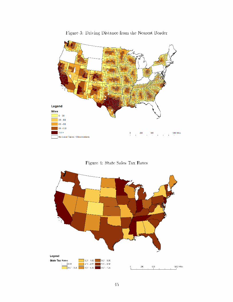
Figure 3: Driving Distance from the Nearest Border

Figure 4: State Sales Tax Rates

45

Figure 5: County Tax Rates by Whether the Nearest Border Is a High- or Low-Tax State

Figure 6: Missouri Example of Local Option Taxes

46

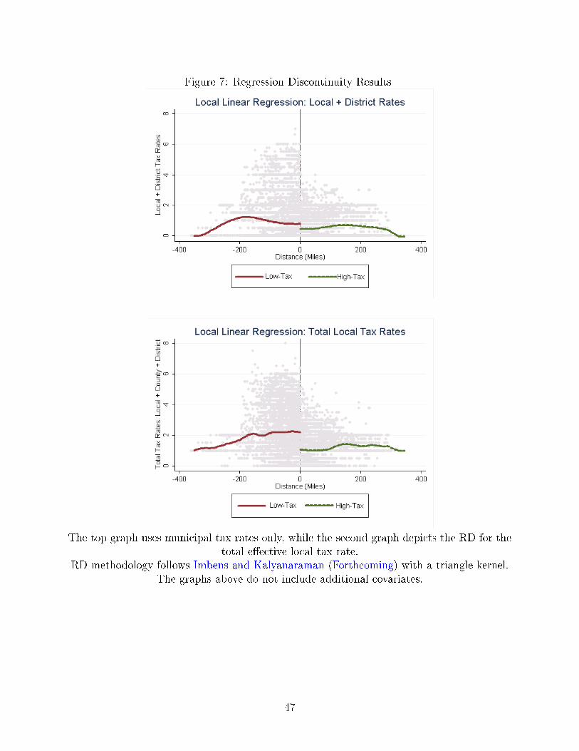
Figure 7: Regression Discontinuity Results

The top graph uses municipal tax rates only, while the second graph depicts the RD for thetotal e�ective local tax rate.

RD methodology follows Imbens and Kalyanaraman (Forthcoming) with a triangle kernel.The graphs above do not include additional covariates.

47

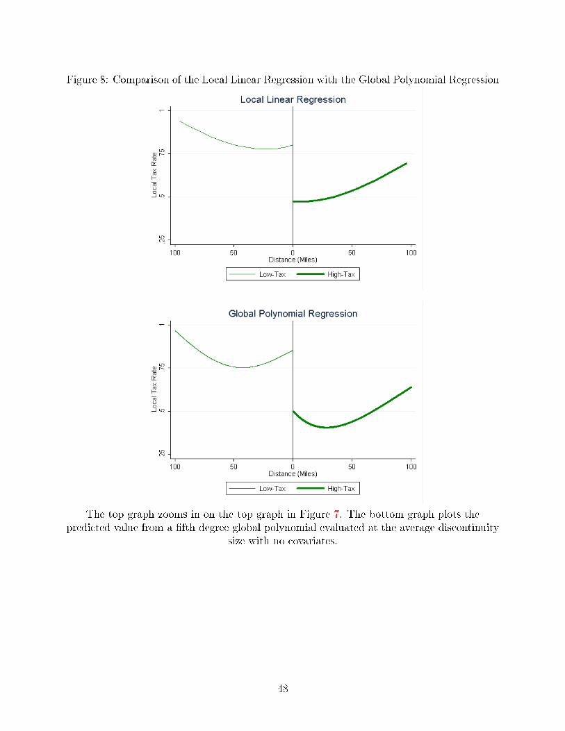
Figure 8: Comparison of the Local Linear Regression with the Global Polynomial Regression

The top graph zooms in on the top graph in Figure 7. The bottom graph plots thepredicted value from a �fth degree global polynomial evaluated at the average discontinuity

size with no covariates.

48

Figure 9: Average Marginal E�ects by Distance, Full Sample

Marginal e�ects represent the e�ect of moving away from the border in both directions.To derive the per mile marginal e�ects, divide by 100.

Con�dence intervals are 95%.

Figure 10: Average Marginal E�ects by Distance, Two States with Same Tax Rate

Marginal e�ects represent the e�ect of moving away from the border in both directions.To derive the per mile marginal e�ects, divide by 100.

Con�dence intervals are 95%.

49

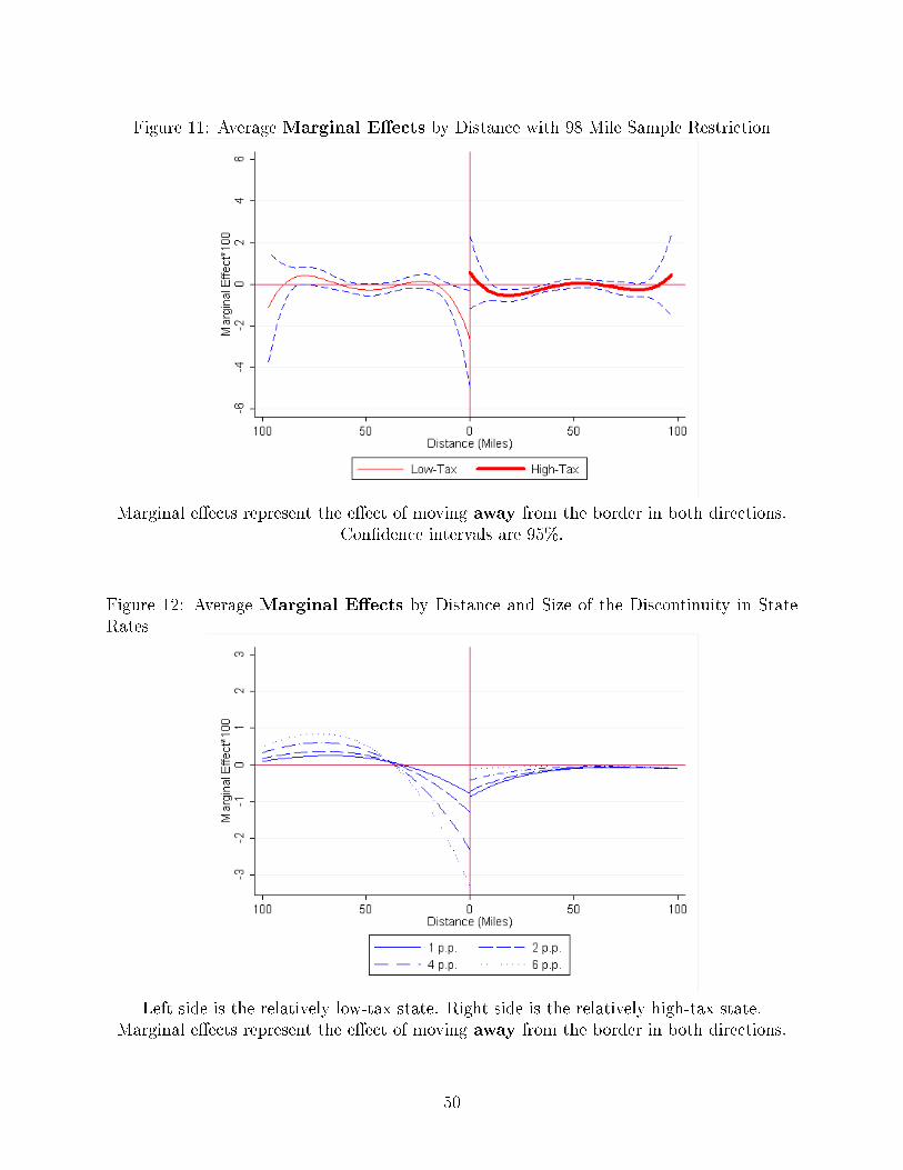
Figure 11: Average Marginal E�ects by Distance with 98 Mile Sample Restriction

Marginal e�ects represent the e�ect of moving away from the border in both directions.Con�dence intervals are 95%.

Figure 12: Average Marginal E�ects by Distance and Size of the Discontinuity in StateRates

Left side is the relatively low-tax state. Right side is the relatively high-tax state.Marginal e�ects represent the e�ect of moving away from the border in both directions.

50

Figure 13: Predicted Values of Local Rates from a Global Polynomial Regression

These graphs plot the predicted values of local tax rates from a global polynomialregression including state �xed e�ects and covariates. The top graph evaluates the

predicted value conditional on the average discontinuity and the set of covariates. Thebottom graph conditions on various discontinuity sizes. The marginal e�ects in Figures 9

and 12 correspond to the slopes of the lines above, respectively.

51

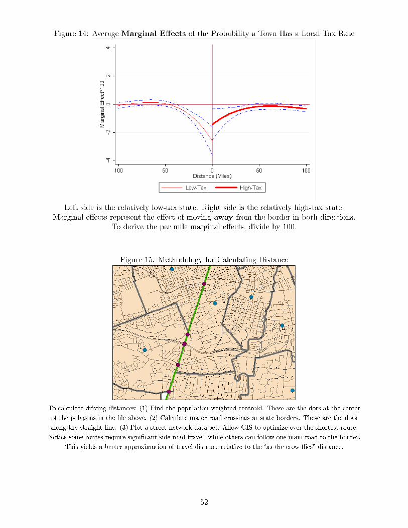
Figure 14: Average Marginal E�ects of the Probability a Town Has a Local Tax Rate

Left side is the relatively low-tax state. Right side is the relatively high-tax state.Marginal e�ects represent the e�ect of moving away from the border in both directions.

To derive the per mile marginal e�ects, divide by 100.

Figure 15: Methodology for Calculating Distance

To calculate driving distances: (1) Find the population weighted centroid. These are the dots at the center

of the polygons in the �le above. (2) Calculate major road crossings at state borders. These are the dots

along the straight line. (3) Plot a street network data set. Allow GIS to optimize over the shortest route.

Notice some routes require signi�cant side road travel, while others can follow one main road to the border.

This yields a better approximation of travel distance relative to the �as the crow-�ies� distance.

52

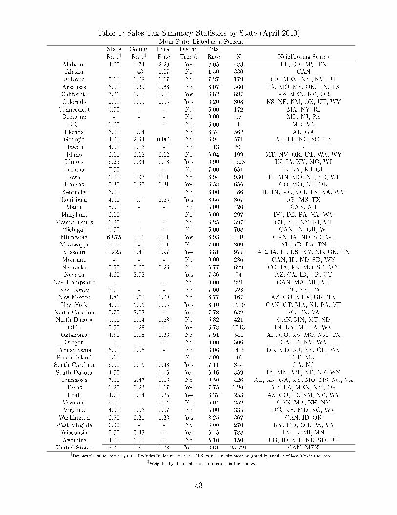
Table 1: Sales Tax Summary Statistics by State (April 2010)Mean Rates Listed as a Percent

StateRate†

CountyRate‡

LocalRate

DistrictTaxes?

TotalRate N Neighboring States

Alabama 4.00 1.74 2.20 Yes 8.05 483 FL, GA, MS, TNAlaska - .43 1.07 No 1.50 330 CANArizona 5.60 1.09 1.17 No 7.27 179 CA, MEX, NM, NV, UTArkansas 6.00 1.39 0.68 No 8.07 560 LA, MO, MS, OK, TN, TXCalifornia 7.25 1.00 0.04 Yes 8.82 897 AZ, MEX, NV, ORColorado 2.90 0.99 2.05 Yes 6.20 308 KS, NE, NM, OK, UT, WY

Connecticut 6.00 - - No 6.00 172 MA, NY, RIDelaware - - - No 0.00 58 MD, NJ, PAD.C. 6.00 - - No 6.00 1 MD, VAFlorida 6.00 0.74 - No 6.74 562 AL, GAGeorgia 4.00 2.94 0.001 No 6.94 571 AL, FL, NC, SC, TNHawaii 4.00 0.13 - No 4.13 66 -Idaho 6.00 0.02 0.02 No 6.04 199 MT, NV, OR, UT, WA, WYIllinois 6.25 0.34 0.13 Yes 6.90 1528 IN, IA, KY, MO, WIIndiana 7.00 - - No 7.00 651 IL, KY, MI, OHIowa 6.00 0.93 0.01 No 6.94 980 IL, MN, MO, NE, SD, WIKansas 5.30 0.97 0.31 Yes 6.58 656 CO, MO, NE, OKKentucky 6.00 - - No 6.00 486 IL, IN, MO, OH, TN, VA, WVLouisiana 4.00 1.71 2.66 Yes 8.66 367 AR, MS, TXMaine 5.00 - - No 5.00 426 CAN, NH

Maryland 6.00 - - No 6.00 297 DC, DE, PA, VA, WVMassachusetts 6.25 - - No 6.25 397 CT, NH, NY, RI, VTMichigan 6.00 - - No 6.00 708 CAN, IN, OH, WIMinnesota 6.875 0.01 0.01 Yes 6.93 1048 CAN, IA, ND, SD, WIMississippi 7.00 - 0.01 No 7.00 309 AL, AR, LA, TNMissouri 4.225 1.40 0.97 Yes 6.81 977 AR, IA, IL, KS, KY, NE, OK, TNMontana - - - No 0.00 236 CAN, ID, ND, SD, WYNebraska 5.50 0.00 0.26 No 5.77 629 CO, IA, KS, MO, SD, WYNevada 4.60 2.72 - Yes 7.36 74 AZ, CA, ID, OR, UT

New Hampshire - - - No 0.00 221 CAN, MA, ME, VTNew Jersey 7.00 - - No 7.00 528 DE, NY, PANew Mexico 4.85 0.62 1.29 No 6.77 167 AZ, CO, MEX, OK, TXNew York 4.00 3.93 0.05 Yes 8.10 1310 CAN, CT, MA, NJ, PA, VT

North Carolina 5.75 2.03 - Yes 7.78 632 SC, TN, VANorth Dakota 5.00 0.04 0.28 No 5.32 421 CAN, MN, MT, SD

Ohio 5.50 1.28 - Yes 6.78 1043 IN, KY, MI, PA, WVOklahoma 4.50 1.08 2.33 No 7.91 544 AR, CO, KS, MO, NM, TXOregon - - - No 0.00 306 CA, ID, NV, WA

Pennsylvania 6.00 0.06 - No 6.06 1418 DE, MD, NJ, NY, OH, WVRhode Island 7.00 - - No 7.00 46 CT, MASouth Carolina 6.00 0.13 0.43 Yes 7.11 344 GA, NCSouth Dakota 4.00 - 1.16 Yes 5.16 359 IA, MN, MT, ND, NE, WYTennessee 7.00 2.47 0.03 No 9.50 426 AL, AR, GA, KY, MO, MS, NC, VATexas 6.25 0.23 1.17 Yes 7.75 1386 AR, LA, MEX, NM, OKUtah 4.70 1.14 0.25 Yes 6.37 253 AZ, CO, ID, NM, NV, WY

Vermont 6.00 - 0.04 No 6.04 252 CAN, MA, NH, NYVirginia 4.00 0.93 0.07 No 5.00 335 DC, KY, MD, NC, WV

Washington 6.50 0.31 1.33 Yes 8.25 367 CAN, ID, ORWest Virginia 6.00 - - No 6.00 270 KY, MD, OH, PA, VAWisconsin 5.00 0.43 - Yes 5.45 788 IA, IL, MI, MNWyoming 4.00 1.10 - No 5.10 150 CO, ID, MT, NE, SD, UT

United States 5.31 0.81 0.38 Yes 6.61 25,721 CAN, MEX†Denotes the state statutory rate. Excludes Indian reservations. U.S. values are the mean weighted by number of localities in the state.

‡Weighted by the number of jurisdictions in the county.

53

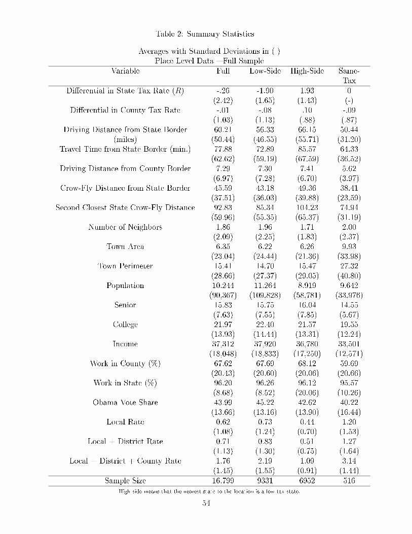
Table 2: Summary Statistics

Averages with Standard Deviations in ( )Place Level Data � Full Sample

Variable Full Low-Side High-Side Same-Tax

Di�erential in State Tax Rate (R) -.26(2.42)

-1.90(1.65)

1.93(1.43)

0(-)

Di�erential in County Tax Rate -.01(1.03)

-.08(1.13)

.10(.88)

-.09(.87)

Driving Distance from State Border(miles)

60.21(50.44)

56.33(46.55)

66.15(55.71)

50.44(31.20)

Travel Time from State Border (min.) 77.88(62.62)

72.89(59.19)

85.57(67.59)

64.33(36.52)

Driving Distance from County Border 7.29(6.97)

7.30(7.28)

7.41(6.70)

5.62(3.97)

Crow-Fly Distance from State Border 45.59(37.51)

43.18(36.03)

49.36(39.88)

38.41(23.59)

Second Closest State Crow-Fly Distance 92.83(59.96)

85.34(55.35)

104.23(65.37)

74.94(31.19)

Number of Neighbors 1.86(2.09)

1.96(2.25)

1.71(1.83)

2.00(2.37)

Town Area 6.35(23.04)

6.22(24.44)

6.26(21.36)

9.93(33.98)

Town Perimeter 15.41(28.66)

14.70(27.37)

15.47(29.05)

27.32(40.80)

Population 10,244(90,367)

11,264(109,828)

8,919(58,781)

9.642(33,976)

Senior 15.83(7.63)

15.75(7.55)

16.04(7.85)

14.55(5.67)

College 21.97(13.93)

22.40(14.44)

21.57(13.31)

19.55(12.24)

Income 37,312(18,048)

37,920(18,833)

36,780(17,250)

33,501(12,571)

Work in County (%) 67.62(20.43)

67.69(20.60)

68.12(20.06)

59.69(20.66)

Work in State (%) 96.20(8.68)

96.26(8.52)

96.12(20.06)

95.57(10.26)

Obama Vote Share 43.99(13.66)

45.22(13.16)

42.62(13.90)

40.22(16.44)

Local Rate 0.62(1.08)

0.73(1.24)

0.44(0.70)

1.20(1.53)

Local + District Rate 0.71(1.13)

0.83(1.30)

0.51(0.75)

1.27(1.64)

Local + District + County Rate 1.76(1.45)

2.19(1.55)

1.09(0.91)

3.14(1.44)

Sample Size 16,799 9331 6952 516High-side means that the nearest state to the location is a low-tax state.

54

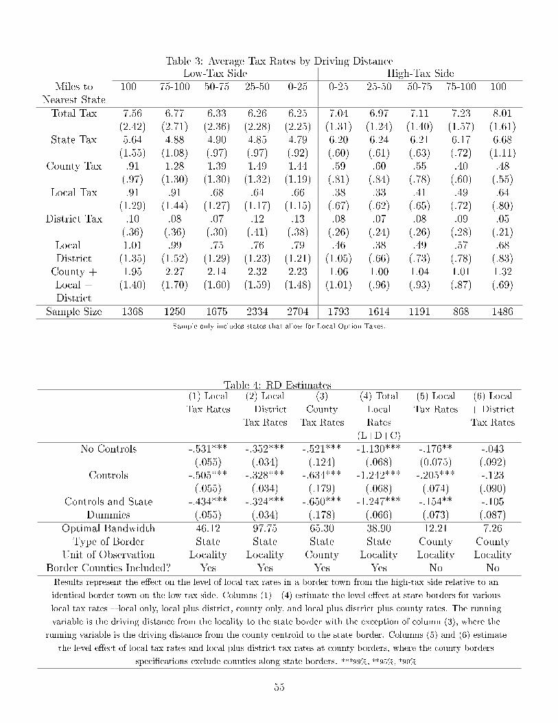
Table 3: Average Tax Rates by Driving DistanceLow-Tax Side High-Tax Side

Miles toNearest State

100+ 75-100 50-75 25-50 0-25 0-25 25-50 50-75 75-100 100+

Total Tax 7.56(2.42)

6.77(2.71)

6.33(2.36)

6.26(2.28)

6.25(2.25)

7.04(1.31)

6.97(1.24)

7.11(1.40)

7.23(1.57)

8.01(1.61)

State Tax 5.64(1.55)

4.88(1.08)

4.90(.97)

4.85(.97)

4.79(.92)

6.20(.60)

6.24(.61)

6.21(.63)

6.17(.72)

6.68(1.11)

County Tax .91(.97)

1.28(1.30)

1.39(1.30)

1.49(1.32)

1.44(1.19)

.59(.81)

.60(.84)

.55(.78)

.40(.60)

.48(.55)

Local Tax .91(1.29)

.91(1.44)

.68(1.27)

.64(1.17)

.66(1.15)

.38(.67)

.33(.62)

.41(.65)

.49(.72)

.64(.80)

District Tax .10(.36)

.08(.36)

.07(.30)

.12(.41)

.13(.38)

.08(.26)

.07(.24)

.08(.26)

.09(.28)

.05(.21)

Local +District

1.01(1.35)

.99(1.52)

.75(1.29)

.76(1.23)

.79(1.21)

.46(1.05)

.38(.66)

.49(.73)

.57(.78)

.68(.83)

County +Local +District

1.95(1.40)

2.27(1.70)

2.14(1.60)

2.32(1.59)

2.23(1.48)

1.06(1.01)

1.00(.96)

1.04(.93)

1.01(.87)

1.32(.69)

Sample Size 1368 1250 1675 2334 2704 1793 1614 1191 868 1486Sample only includes states that allow for Local Option Taxes.

Table 4: RD Estimates(1) Local

Tax Rates

(2) Local

+ District

Tax Rates

(3)

County

Tax Rates

(4) Total

Local

Rates

(L+D+C)

(5) Local

Tax Rates

(6) Local

+ District

Tax Rates

No Controls -.531***(.055)

-.352***(.034)

-.521***(.124)

-1.130***(.068)

-.176**(0.075)

-.043(.092)

Controls -.505***(.055)

-.328***(.034)

-.634***(.179)

-1.242***(.068)

-.205***(.074)

-.123(.090)

Controls and StateDummies

-.434***(.055)

-.324***(.034)

-.650***(.178)

-1.247***(.066)

-.154**(.073)

-.105(.087)

Optimal Bandwidth 46.12 97.75 65.30 38.90 12.21 7.26Type of Border State State State State County County

Unit of Observation Locality Locality County Locality Locality LocalityBorder Counties Included? Yes Yes Yes Yes No NoResults represent the e�ect on the level of local tax rates in a border town from the high-tax side relative to an

identical border town on the low-tax side. Columns (1) - (4) estimate the level e�ect at state borders for various

local tax rates � local only, local plus district, county only, and local plus district plus county rates. The running

variable is the driving distance from the locality to the state border with the exception of column (3), where the

running variable is the driving distance from the county centroid to the state border. Columns (5) and (6) estimate

the level e�ect of local tax rates and local plus district tax rates at county borders, where the county borders

speci�cations exclude counties along state borders. ***99%, **95%, *90%

55

Table 5: Regression Coe�cients for the Estimating EquationVariable (1) (2) (3) (4)Same (S) .560

(.403).640*(.375)

.403**(.162)

.350**(.145)

High (H) .066(.095)

.240***(.089)

.226***(.060)

.209***(.062)

Notch (R) -.174***(.039)

-.347***(.038)

-.095***(.025)

-.118***(.025)

H ·R .129***(.045)

.302***(.043)

.027(.030)

.063**(.030)

Distance (d) 1.346**(.643)

1.394**(.628)

-.227(.384)

.279(.414)

S · d -.8168(-7.033)

-8.445(6.497)

-4.541(2.878)

-3.626(2.599)

H · d -1.436*(.843)

-.578(.800)

-.810(.532)

-1.294**(.554)

R · d .888***(.295)

.766***(.285)

.443***(.168)

.508***(.166)

H ·R · d -1.246***(.355)

-1.283***(.343)

-.344(.215)

.358*(.211)

d2 -4.137**(1.709)

-3.051*(1.698)

.228(1.040)

-.705(1.087)

S · d2 61.003(37.526)

62.433*(34.504)

28.903*(15.979)

22.476(14.447)

H · d2 2.853(-2.298)

-.081(2.197)

1.277(1.455)

2.592*(1.501)

R · d2 -2.077***(.719)

-1.457**(.715)

-.895**(.429)

-.993**(.425)

H ·R · d2 3.733***(.891)

3.383***(.870)

.991*(.549)

.711(.542)

d3 5.295***(1.811)

3.079*(1.843)

-.082(1.131)

.404(1.152)

S · d3 -158.815*(81.579)

-158.969**(74.585)

-66.955*(35.64)

-54.118*(32.082)

H · d3 -3.493(2.492)

.165(2.395)

-1.09(1.582)

-2.193(1.611)

R · d3 2.059***(.726)

.993(.742)

.679(.454)

.652(.449)

H ·R · d3 -3.747***(.913)

-2.837***(.898)

-.870(.573)

-.371(.572)

d4 -2.491***(.802)

-1.170(.844)

.055(.517)

.010(.519)

S · d4 168.433**(76.777)

164.557**(69.842)

64.788*(34.107)

54.247*(30.510)

H · d4 1.923*(1.132)

.053(1.096)

.387(.722)

.769(.730)

R · d4 -.850***(.315)

-.273.332

-.203(.205)

-.147(.203)

H ·R · d4 1.425***(.400)

.910(.398)

.281(.255)

.012(.257)

56

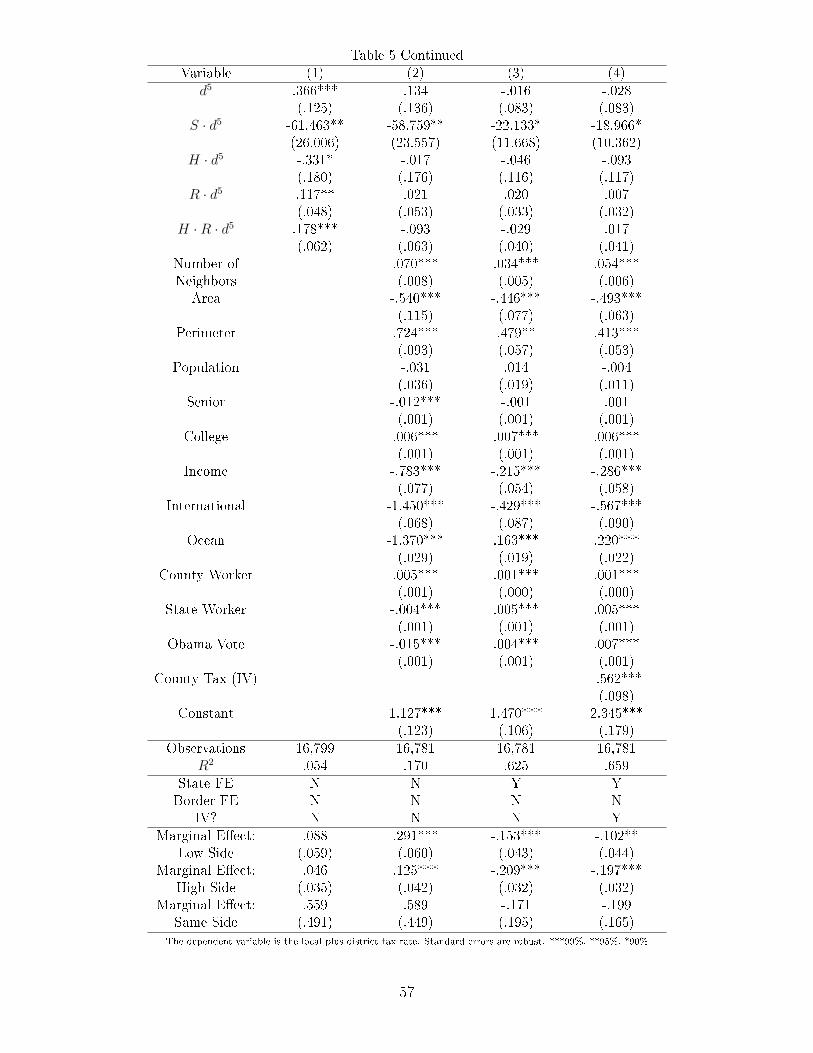
Table 5 ContinuedVariable (1) (2) (3) (4)

d5 .366***(.125)

.134(.136)

-.016(.083)

-.028(.083)

S · d5 -61.463**(26.006)

-58.759**(23.557)

-22.133*(11.668)

-18.966*(10.362)

H · d5 -.331*(.180)

-.017(.176)

-.046(.116)

-.093(.117)

R · d5 .117**(.048)

.021(.053)

.020(.033)

.007(.032)

H ·R · d5 .178***(.062)

-.093(.063)

-.029(.040)

.017(.041)

Number ofNeighbors

.070***(.008)

.034***(.005)

.054***(.006)

Area -.540***(.115)

-.446***(.077)

-.493***(.063)

Perimeter .724***(.093)

.479**(.057)

.413***(.053)

Population -.031(.036)

.014(.019)

-.004(.011)

Senior -.012***(.001)

-.001(.001)

.001(.001)

College .006***(.001)

.007***(.001)

.006***(.001)

Income -.783***(.077)

-.215***(.054)

-.286***(.058)

International -1.450***(.068)

-.429***(.087)

-.567***(.090)

Ocean -1.370***(.029)

.163***(.019)

.220***(.022)

County Worker .005***(.001)

.001***(.000)

.001***(.000)

State Worker -.004***(.001)

.005***(.001)

.005***(.001)

Obama Vote -.015***(.001)

.004***(.001)

.007***(.001)

County Tax (IV) -.562***(.098)

Constant 1.127***(.123)

1.470***(.106)

2.345***(.179)

Observations 16,799 16,781 16,781 16,781R2 .054 .170 .625 .659

State FE N N Y YBorder FE N N N N

IV? N N N YMarginal E�ect:

Low Side.088(.059)

.291***(.060)

-.153***(.043)

-.102**(.044)

Marginal E�ect:High Side

.046(.035)

.125***(.042)

-.209***(.032)

-.197***(.032)

Marginal E�ect:Same Side

.559(.491)

.589(.449)

-.171(.195)

-.199(.165)

The dependent variable is the local plus district tax rate. Standard errors are robust. ***99%, **95%, *90%

57

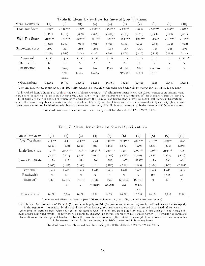
Table 6: Mean Derivatives for Several Speci�cationsMean Derivative (1) (2) (3) (4) (5) (6) (7) (8) (9) (10)

Low-Tax State -.103**

(.044)

-.116***

(.042)

-.133**

(.058)

-.240***

(.058)

-.055***

(.015)

-.094**

(.049)

-.086

(.070)

-.286***

(.054)

-.135**

(.064)

-.077*

(.041)

High-Tax State -.197***

(.032)

-.181***

(.030)

-.198***

(.033)

-.211***

(.039)

-.102***

(.014)

-.209***

(.035)

-.239***

(.041)

+.097*

(.058)

-.113***

(.034)

-.179***

(.032)

Same-Tax State -.199

(.165)

-.227

(.162)

-.198

(.164)

-.186

(.167)

-.045

(.069)

-.185

(.174)

-.204

(.210)

-.126

(.123)

-.221

(.198)

-.107

(.144)

Variable† L+D L+D L+D L+D L+D L+D L+D L+D L L+D+C

Bandwidth N N N N N N N N N N

Restriction N Binary

Treat-

ment

No

Intern.

No

Ocean

Time MS, NC,

NV, WI

Nbr.

LOST

Nbr. No

LOST

N N

Observations 16,781 16,781 15,642 14,255 16,781 15243 12,516 3126 14,563 16,781

The marginal e�ects represent a per 100 mile change (i.e., per mile, the units are basis points), except for (5), which is per hour.

(1) is derived from column 4 of Table 5. (2) uses a binary treatment. (3) eliminates towns where the closest border is an internationalone. (4) eliminates towns proximate to the ocean. (5) uses driving time instead of driving distance. (6) drops states where the primarylocal taxes are district taxes. (7) utilizes only towns where the nearest neighboring state allows for LOST. (8) includes observations

where the nearest neighbor is a state that does not allow LOST. (9) uses local taxes as the left side variable. (10) uses city plus districtplus county taxes as the left-side variable and controls for the county X's. †L is local taxes, D is district taxes, and C is county taxes.

Standard errors are robust and calculated using the Delta Method. ***99%, **95%, *90%.

Table 7: Mean Derivatives for Several Speci�cations

Mean Derivative (1) (2) (3) (4) (5) (6) (7) (8) (9) (10)

Low-Tax State -.103**

(.044)

-.049

(.030)

-.083**

(.046)

-.051

(.045)

-.704***

(.152)

-.203***

(.072)

-.203***

(.070)

-.118**

(.054)

-.180**

(.094)

-.695*

(.398)

High-Tax State -.197***

(.032)

-.150***

(.024)

-.181***

(.031)

-.169***

(.031)

-.230***

(.061)

-.129**

(.058)

-.490***

(.149)

-.190***

(.041)

-.194***

(.072)

-.490

(.330)

Same-Tax State -.199

(.165)

-.012

(.128)

-.212

(.149)

-.204

(.161)

-.513

(.460)

-.486*

(.251)

-.380**

(.179)

-.199

(.167)

-.395

(.342)

-.051

(2.616)

Variable† L+D L+D L+D L+D L+D L+D L+D L+D L+D L+D

Bandwidth N N N N N N N 152 97.75 40

Restrict? No Degree

3

Degree

7

State

Weights

Pop.

Weights

Interact

All

Border

& St.

FE

N N N

Observations 16,781 16,781 16,781 16,781 16,781 16,781 16,781 16,124 13,739 7236

The marginal e�ects represent a per 100 mile change (i.e., per mile, the units are basis points).

(1) is derived from column 4 of Table 5. (2) uses a cubic polynomial. (3) uses an order seven polynomial. (4) weights each state equallyin the regression. (5) weights by the population of the locality. (6) interacts the control variables and state �xed e�ects with a

polynomial in distance along with a full set of interactions with the high- and same-side dummies. (7) includes state �xed e�ects andstate-border-pair �xed e�ects. (8) restricts the sample to observations within 150 miles of the nearest border. (9) restricts the sample toobservations within the optimal bandwidth from the local linear regression. (10) restricts the sample to observations within forty miles

of the nearest border. †L is local taxes, D is district taxes, and C is county taxes.

Standard errors are robust and calculated using the Delta Method. ***99%, **95%, *90%

58

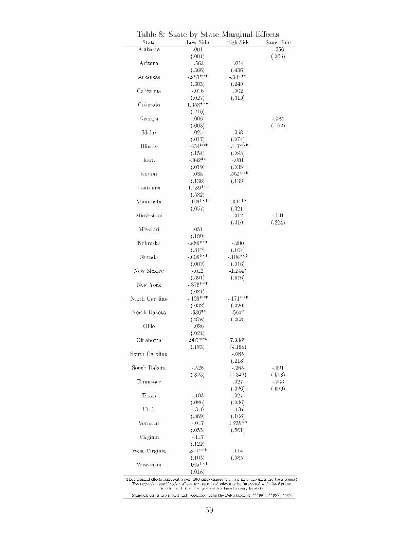
Table 8: State by State Marginal E�ectsState Low Side High Side Same Side

Alabama .001(.001)

-.056(.366)

Arizona -.563(.366)

-.014(.436)

Arkansas -.981***(.303)

-.544**(.249)

California -.016(.027)

.002(.019)

Colorado 1.358***(.210)

Georgia .006(.008)

-.084(.162)

Idaho .025(.017)

.058(.074)

Illinois -.434***(.154)

-.517***(.093)

Iowa -.042**(.019)

-.001(.038)

Kansas .038(.136)

-.555***(.136)

Louisiana -1.189***(.382)

Minnesota -.199***(.057)

-.041**(.021)

Mississippi .012(.010)

-.131(.224)

Missouri .051(.190)

Nebraska -.880***(.312)

-.200(.164)

Nevada -.008***(.002)

-.108***(.016)

New Mexico -.012(.391)

-1.244*(.676)

New York -.378***(.081)

North Carolina -.139***(.032)

-.171***(.020)

North Dakota -.636**(.278)

.564*(.308)

Ohio -.026(.024)

Oklahoma .905***(.183)

7.936*(4.198)

South Carolina -.085(.218)

South Dakota -.528(.325)

-.265(1.342)

-.591(.513)

Tennessee .027(.026)

-.003(.069)

Texas -.103(.086)

.027(.036)

Utah -.310(.369)

-.137(.106)

Vermont -.017(.055)

1.235**(.561)

Virginia -.117(.122)

West Virginia .311***(.103)

.114(.085)

Wisconsin -.095***(.018)

The marginal e�ects represent a per 100 mile change (i.e., per mile, the units are basis points).The regression speci�cation allows for state �xed e�ects to be interacted with the distance

function such that the gradient is allowed to vary by state.

Standard errors are robust and calculated using the Delta Method. ***99%, **95%, *90%

59

Table 9: Average Marginal E�ects by Size of the Treatment/DiscontinuitySpeci�cation IV Regression of Rates Probit Binary Variable

Low-TaxSide

High-TaxSide

Same-Tax

Low-TaxSide

High-TaxSide

Same-Tax

Not Conditioned on Notch(R)

-.103**(.044)

-.197***(.032)

-.199(.165)

-.469***(.087)

-.435***(.092)

-.135(.467)

5th Percentile of RRLow = −.25 ; RHigh = .25

-.029(.059)

-.234***(.049)

-.348***(.126)

-.663***(.119)

10th Percentile of RRLow = −.50 ; RHigh = .25

-.041(.055)

-.234***(.049)

-.365***(.118)

-.663***(.119)

20th Percentile of RRLow = −.75 ; RHigh = .875

-.054(.051)

-.217***(.041)

-.382***(.110)

-.571***(.102)

30th Percentile of RRLow = −.875 ; RHigh = 1.25

-.060(.050)

-.206***(.037)

-.391***(.106)

-.516***(.096)

40th Percentile of RRLow = −1.25 ; RHigh = 1.75

-.079*(.046)

-.192***(.033)

-.416***(.097)

-.443***(.095)

50th Percentile of RRLow = −1.75 ; RHigh = 1.75

-.105**(.044)

-.192***(.033)

-.450***(.090)

-.443***(.095)

60th Percentile RRLow = −2 ; RHigh = 1.875

-.117***(.045)

-.189***(.032)

-.467***(.088)

-.424***(.096)

70th Percentile of RRLow = −2 ; RHigh = 2.025

-.117***(.045)

-.185***(.032)

-.467***(.088)

-.402***(.097)

80th Percentile of RRLow = −2.75 ; RHigh = 2.25

-.155***(.052)

-.178***(.032)

-.518***(.095)

-.369***(.101)

90th Percentile of RRLow = −3 ; RHigh = 3.65

-.168***(.056)

-.139***(.040)

-.534***(.101)

-.163(.146)

95th Percentile of RRLow = −5.125 ; RHigh = 6

-.275***(.102)

-.073(.073)

-.678***(.179)

.183(.256)

The marginal e�ects represent a per 100 mile change (i.e., per mile, the units are basis points).

Standard Errors are robust and calculated using the Delta Method. ***99%, **95%, *90%

Table 10: Mean Derivatives for Multiple Borders

Mean Derivative (1) (2) (3) (4) (5)

Low-Tax State -.069

(.065)

-.127**

(.065)

.029

(.067)

-.461

(.458)

-.396

(.462)

High-Tax State -.181***

(.043)

-.189***

(.044)

-.129**

(.061)

-1.060**

(.417)

-1.206***

(.410)

Same-Tax State -.111

(0.192)

-.162

(.193)

.010

(.192)

-1.003***

(.174)

-.935***

(.173)

Marginal E�ects State State State County County

1st State Y Y Y N Y

2nd State N Y Y N Y

County Border N N Y Y Y

Border Counties? Y Y Y N Y

The marginal e�ects represent a per 100 mile change (i.e., per mile, the units are basis points).

(1) is derived from column (4) of Table 5 but uses the �as the crow-�ies� distance. (2) adds a polynomial in distance from the

second border plus interactions. (3) uses polynomials in distance from the closest state border, the second closest state border

and the closest county border plus the appropriate interactions. (4) includes a polynomial to the closest county border and

drops state border counties. (5) is the same as (3) but calculates marginal e�ects from the county border.

Standard errors are robust and calculated using the Delta Method. ***99%, **95%, *90%

60