The system and its model - UofG Computingdobo/2460/models-1.pdfCIS 2460 Modelling of Computer...

CIS 2460 Modelling of Computer Systems'

&

$

%

The system and its model

The standard assumption is that the “system” starts its

operation at time 0 and works forever. Thus we will not know

the true properties of the system until the end of time

(whatever that means).

In a model, we use the information gathered as modelling

time progresses, i.e. from time 0 to time T (T is just a

symbolic notation).

The model yields some statistics; if the model was properly

constructed, the larger T is, the closer these statistics are to

the real ones.

If the model contains errors, its statistics will never converge

to real values–this is a serious problem because a bad

model looks as good as a good model until proven

otherwise.

1


&

$

%

Models

There are two ways to model a system:

• Mathematical models , mainly “Queuing Theory” apply

to client–server systems.

Pros : easy to use (once you know Q.T.) and results can

be obtained in a couple of minutes without any

programming. Moreover, there is no need to validate

the results because famous mathematicians already

proved them correct.

Cons : many simplifications, some activities cannot be

modelled. Consequently, some statistics cannot be

obtained.

2


&

$

%

• Statistical models —can model any kind of systems.

Pros : anything you wish can be modelled using a

statistical model and computer simulation. Deep

theoretical knowledge is not needed; only

programming and Statistics.

Cons : a simulator has to be written. Many decisions

must be made about the pdf’s to be used in various

components of the model. Most importantly, the

results must be validated and even then are not fully

trustworthy (“19 times out of 20”).

3


&

$

%

Queuing theory

QT models systems with servers and clients (presumably

waiting in queues ). Elements of the theory will be covered in

greater detail at a later time; now is the time for a brief

preview.

Notation: there are many standard symbols like

λ, µ, ρ, An, Wn, L(t), L, LQ, w, wQ etc. These

represent the actual properties of a system. There is no

need to know the meaning of all of them now.

The interpretation is simple: a “hat” on top of a symbol, such

as L says that this is an approximate value of L called an

estimator . Note that the exact value of L will never be

known to anyone.

4


&

$

%

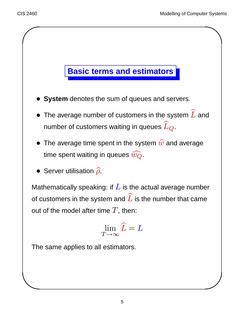
Basic terms and estimators

• System denotes the sum of queues and servers.

• The average number of customers in the system L and

number of customers waiting in queues LQ.

• The average time spent in the system w and average

time spent waiting in queues wQ.

• Server utilisation ρ.

Mathematically speaking: if L is the actual average number

of customers in the system and L is the number that came

out of the model after time T , then:

limT→∞

L = L

The same applies to all estimators.

5


&

$

%

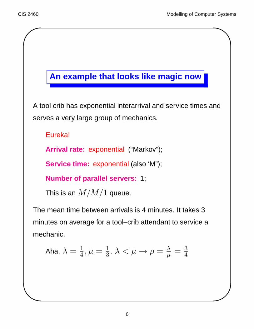
An example that looks like magic now

A tool crib has exponential interarrival and service times and

serves a very large group of mechanics.

Eureka!

Arrival rate: exponential (“Markov”);

Service time: exponential (also ‘M”);

Number of parallel servers: 1;

This is an M/M/1 queue.

The mean time between arrivals is 4 minutes. It takes 3

minutes on average for a tool–crib attendant to service a

mechanic.

Aha. λ = 14 , µ = 1

3 . λ < µ → ρ = λµ

= 34

6


&

$

%

Single attendant

The attendant in paid $10/hour and the mechanic is paid

$15/hour.

The tool crib is a system with one server. The average

waiting time is 1µ(1−ρ) = 12 minutes.

12 minutes of a mechanic’s time are worth $3.

15 mechanics arrive per hour, hence the hourly cost of the

system is: $10 + 15 × $3 = $55/hour.

7


&

$

%

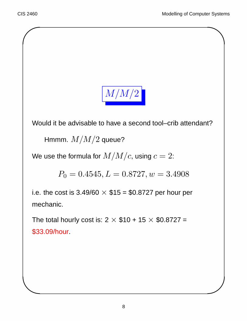
M/M/2

Would it be advisable to have a second tool–crib attendant?

Hmmm. M/M/2 queue?

We use the formula for M/M/c, using c = 2:

P0 = 0.4545, L = 0.8727, w = 3.4908

i.e. the cost is 3.49/60 × $15 = $0.8727 per hour per

mechanic.

The total hourly cost is: 2 × $10 + 15 × $0.8727 =

$33.09/hour.

8


&

$

%

Simulation models

There are four basic types of models.

• Physical models.

• Client–server (queuing systems).

• Inventory systems.

• Reliability modelling.

9


&

$

%

Physical models

This is a broad category of models of physical reality. Some

examples:

1. Behaviour of an eco–system (as a function of time).

2. Mutations in organisms (as a function of generation).

3. Resistance of an object to external phenomena (CPU

chip to temperature variations, etc.).

4. Properties of a digital signal sent over some carrier

(SNR, attenuation, etc.).

some of these models are deterministic; other are

stochastic.

10


&

$

%

Client–server

In client–server systems, the basic notions are:

• Service times, which can be constant or random. If they

are random, good fitting is needed (there are many

different choices). For independent server systems, the

leading candidate is the triangular distribution; for

assembly lines, the Erlang distribution is most

appropriate.

• Customer arrivals, given as interarrival times. Arrivals

usually are modelled by a Poisson process, although the

Gamma (Erlang) distribution often is more useful.

• Queues of waiting customers. One important parameter

is the maximum queue size. In simulation, it is critical to

handle the contents of the queue when a simulation run

ends.

11


&

$

%

Inventory systems

The basic concepts are:

• The size of orders and their frequency. The geometric

distribution and the Poisson process are most often

used.

• The lead time (the time elapsing before an order is

filled). It is widely believed that lead times follow the

Erlang or Weibull distributions.

12


&

$

%

Reliability

Reliability studies focus on determining the mean time

between failures. They rely heavily on Statistics to model the

elusive failure pdf s of the components of the system under

investigation.

A large variety of distributions are used to model failing

components and Queuing Theory is often used in modelling

reliability. This is seldom correct because QT has no means

of taking into account changes of conditions of operation

such as temperature oscillations.

13


&

$

%

Simulation

is the imitation of the operation of a real–world system.

Simulation is a form of modelling and offers all the other

possibilities of making errors; it adds another aspect of

uncertainty: when a simulator models the behaviour of a

system, it gives only a finite number of snapshots of the

states of the system being simulated. Even if these

snapshots are perfect (seldom the case), they do not reflect

the whole complexity of the system (e.g. try reconstructing

the surface of the Moon based on n photographs, for

different values of n).

Warning: simulation may be misleading and should be used

with caution.

14


&

$

%

When to simulate

Answer: whenever you need to know and other methods are

not adequate.

When not to simulate

• When you don’t know enough to build a trustworthy

model.

• If you don’t know Statistics well enough to make sense

out of the results of simulation (sadly, a most common

error).

• When you don’t really know which scenarios/results

matter.

• When the problem is so simple that it can be solved by

another method (prototype, some thinking, queuing

theory, etc.). Other methods are always more

trustworthy when they work.

15


&

$

%

Types of simulation models

There are several ways of classifying simulation models:

• With respect to the stochastic behaviour of some

simulator variables.

• With respect to the flow of time.

All simulation models depend on input parameters. When

randomness or time are involved, they also change

simulation output.

16


&

$

%

Randomness

A simulation model may assume that all events occur

according to a predetermined schedule or it may assume

that some events are subject to random influences.

Deterministic: no randomness involved; the simulator

output always the same.

An example would be to study the behaviour of a

container port facility, where we assume that all the

activities occur according to schedule and are looking

for bottlenecks in the system.

Stochastic: Some simulator variables take as values

random variates (drawn from appropriate probability

distributions).

Any serious model involving servers and customers is

stochastic, because customers arrive (somewhat)

unpredictably and service times vary.

17


&

$

%

Flow of time

Time is an important consideration in simulating a system.

There are two types of models:

Static: when time does not change during simulation (more

exactly: the time change is not recorded during

simulation)

Example: finding an equilibrium (or steady state) in a

complex physical system.

Dynamic: when time flows explicitly during simulation and

its flow drives the behaviour of the simulator. Dynamic

models can be further subdivided into two groups:

1. Continuous—time is supposed to flow continuously

(within the limitations of using a digital computer).

2. Discrete—time does not “flow” but “jumps” from time

value to time value based on the occurrence of

events.

18


&

$

%

Interesting models

In this course, we deal with models that are:

• Discrete,

• Stochastic,

• Dynamic.

Such models are driven by actions called “events” which

occur at specific (discrete) random (stochastic) moments

(dynamic).

19


&

$

%

Why events?

There are two approaches to dynamic simulation:

time–driven (“continuous”) and event–driven (“discrete”).

Continuous simulation is an attempt to mimic reality which

has a dimension called time flowing “continuously” forward.

Continuous simulators are easier to write, but are often

impractical, because of huge execution times.

Discrete simulators are more versatile, but less intuitive.

20


&

$

%

Continuous simulator

A time–driven simulator essentially simulates a real–life

clock.

A “continuous” simulator has an integer variable

representing the current time:

for( int clock = 0 ; clock < END ; clock++ ) {

check if there is work at time "clock"

if so, do what needed.

}

The constant END gives the duration of simulation

expressed as a multiple of a unit called tick and the clock

changes (“ticks”) one tick at a time (second, hour, µs).

21


&

$

%

Continuous

Continuous simulation is the way to go, if:

• There is work almost every tick.

• It takes little time to find what the nature of the work is.

• It is acceptable that time takes only integer values.

Simulation of a CPU is an excellent example of a case when

continuous simulation is the only reasonable way to proceed.

22


&

$

%

Discrete simulation

Instead of simulating a clock, discrete simulation simulates

the occurrence of events.

An event is an instantaneous occurrence that changes

the state of the system (such as the arrival of a new

customer).

Since the state of the system changes only as a result of an

event, nothing changes at moments when no events occur.

Such moments are skipped by the simulator and time

advances not “continuously” (a tick at a time) but discretely

jumps forward from the time of the occurrence of one event

to the time of the occurrence of the next event.

It is critical to process events in order (keep time moving

forward).

23


&

$

%

When discrete

Discrete simulation is the way to go if continuous simulation

is not adequate, i.e. at least one of the following is true:

• No events occur during long periods of time.

• The system is so complex that it takes time to find where

the action is.

• The granularity of time must be fine compared to the

simulation length.

The simulation of a packet–oriented network connection is

an example of an application of discrete simulation.

24


&

$

%

Carwash example

A simplistic model of a single–car washing station:

1. A car arrives to the carwash (this is an event).

2. Washing starts (this is an event).

3. Washing in progress (this is not an event).

4. Washing ends (this is an event).

5. Car exits. This is an event that may be incorporated in

the model to capture the situation when a car that has

already been washed remains inside the carwash

station preventing the next car from entering it.

25

The system and its model - UofG Computingdobo/2460/models-1.pdfCIS 2460 Modelling of Computer...

Documents

Transcript of The system and its model - UofG Computingdobo/2460/models-1.pdfCIS 2460 Modelling of Computer...