
The superconductor-metal quantum phase transition in ultra ...
192
The superconductor-metal quantum phase transition in ultra-narrow wires A dissertation presented by Adrian Giuseppe Del Maestro to The Department of Physics in partial fulfillment of the requirements for the degree of Doctor of Philosophy in the subject of Physics Harvard University Cambridge, Massachusetts May 2008
Transcript of The superconductor-metal quantum phase transition in ultra ...

The superconductor-metal quantum phasetransition in ultra-narrow wires
A dissertation presented
by
Adrian Giuseppe Del Maestro
to
The Department of Physics
in partial fulfillment of the requirements
for the degree of
Doctor of Philosophy
in the subject of
Physics
Harvard University
Cambridge, Massachusetts
May 2008

c©2008 - Adrian Giuseppe Del Maestro
All rights reserved.

Thesis advisor AuthorSubir Sachdev Adrian Giuseppe Del Maestro
The superconductor-metal quantum phase transition in ultra-narrow wires
AbstractWe present a complete description of a zero temperature phase transition betweensuperconducting and diffusive metallic states in very thin wires due to a Cooper pairbreaking mechanism originating from a number of possible sources. These includeimpurities localized to the surface of the wire, a magnetic field orientated parallelto the wire or, disorder in an unconventional superconductor. The order parameterdescribing pairing is strongly overdamped by its coupling to an effectively infinitebath of unpaired electrons imagined to reside in the transverse conduction channelsof the wire. The dissipative critical theory thus contains current reducing fluctuationsin the guise of both quantum and thermally activated phase slips. A full cross-overphase diagram is computed via an expansion in the inverse number of complex com-ponents of the superconducting order parameter (equal to one in the physical case).The fluctuation corrections to the electrical and thermal conductivities are deter-mined, and we find that the zero frequency electrical transport has a non-monotonictemperature dependence when moving from the quantum critical to low tempera-ture metallic phase, which may be consistent with recent experimental results onultra-narrow MoGe wires. Near criticality, the ratio of the thermal to electrical con-ductivity displays a linear temperature dependence and thus the Wiedemann-Franzlaw is obeyed. We compute the constant of proportionality in a systematic expansionand find a universal and experimentally verifiable fluctuation correction to the Lorenznumber.
In the presence of quenched disorder, a novel algorithm is developed to solve theself-consistency condition arising when the number of complex order parameter com-ponents is taken to be large. In this limit, we find striking evidence for the flowto infinite randomness, and observe dynamically activated scaling consistent withpredictions from the strong disorder renormalization group. Moreover, the infiniterandomness fixed point of the pair-breaking superconductor-metal quantum phasetransition is found to be in the same universality class as the onset of ferromagnetismin the one dimensional quantum Ising model in a random transverse field. This discov-ery may lead to the first calculations of real electrical transport in an experimentallyrelevant system exhibiting infinite randomness.
iii

Contents
Citations to Previously Published Work . . . . . . . . . . . . . . . . . . . viiAcknowledgments . . . . . . . . . . . . . . . . . . . . . . . . . . . . . . . . ixDedication . . . . . . . . . . . . . . . . . . . . . . . . . . . . . . . . . . . . xi
1 Introduction 11.1 Superconductivity . . . . . . . . . . . . . . . . . . . . . . . . . . . . . 2
1.1.1 BCS theory . . . . . . . . . . . . . . . . . . . . . . . . . . . . 41.2 Fluctuations in low dimensional superconductors . . . . . . . . . . . . 8
1.2.1 LAMH theory . . . . . . . . . . . . . . . . . . . . . . . . . . . 91.3 Ultra narrow wires . . . . . . . . . . . . . . . . . . . . . . . . . . . . 14
1.3.1 Evidence for quantum phase slips . . . . . . . . . . . . . . . . 141.3.2 Suspended molecular templating . . . . . . . . . . . . . . . . . 14
1.4 Pair-breaking theory . . . . . . . . . . . . . . . . . . . . . . . . . . . 171.4.1 Magnetic fields and impurities . . . . . . . . . . . . . . . . . . 181.4.2 Experimental manifestations . . . . . . . . . . . . . . . . . . . 21
1.5 Quantum phase transitions . . . . . . . . . . . . . . . . . . . . . . . . 261.5.1 Landau theory . . . . . . . . . . . . . . . . . . . . . . . . . . 261.5.2 The scaling hypothesis . . . . . . . . . . . . . . . . . . . . . . 281.5.3 Quantum statistical mechanics . . . . . . . . . . . . . . . . . . 291.5.4 Quantum critical phenomena . . . . . . . . . . . . . . . . . . 331.5.5 Finite temperature crossovers . . . . . . . . . . . . . . . . . . 35
1.6 Disordered critical phenomena . . . . . . . . . . . . . . . . . . . . . . 381.6.1 The Harris criterion . . . . . . . . . . . . . . . . . . . . . . . . 391.6.2 Spin Glasses . . . . . . . . . . . . . . . . . . . . . . . . . . . . 411.6.3 Rare region effects . . . . . . . . . . . . . . . . . . . . . . . . 43
1.7 Organization . . . . . . . . . . . . . . . . . . . . . . . . . . . . . . . 46
2 Dissipative Theory of the Superconductor-Metal Transition 472.1 Dissipative model . . . . . . . . . . . . . . . . . . . . . . . . . . . . . 502.2 Scaling analysis . . . . . . . . . . . . . . . . . . . . . . . . . . . . . . 522.3 Particle-hole asymmetry . . . . . . . . . . . . . . . . . . . . . . . . . 552.4 Phase fluctuations . . . . . . . . . . . . . . . . . . . . . . . . . . . . . 572.5 Connection to microscopic BCS theory . . . . . . . . . . . . . . . . . 59
iv
Contents v
2.5.1 Pair-breaking in quasi-one dimensional wires . . . . . . . . . . 592.5.2 Microscopic parameters in the clean and dirty limits . . . . . . 60
2.6 Universality in the quantum critical regime . . . . . . . . . . . . . . . 622.7 The role of disorder . . . . . . . . . . . . . . . . . . . . . . . . . . . . 66
3 Thermoelectric Transport in the Large-N Limit 683.1 Previous transport results . . . . . . . . . . . . . . . . . . . . . . . . 68
3.1.1 LAMH theory . . . . . . . . . . . . . . . . . . . . . . . . . . . 693.1.2 Microscopic theory . . . . . . . . . . . . . . . . . . . . . . . . 70
3.2 Finite temperature dynamics . . . . . . . . . . . . . . . . . . . . . . . 703.2.1 Effective classical theory . . . . . . . . . . . . . . . . . . . . . 723.2.2 Classical conductivity . . . . . . . . . . . . . . . . . . . . . . . 78
3.3 The ordered phase . . . . . . . . . . . . . . . . . . . . . . . . . . . . 813.3.1 Zero temperature effective potential . . . . . . . . . . . . . . . 823.3.2 Construction of a Ginzburg-Landau potential . . . . . . . . . 863.3.3 Free energy barrier height and LAMH theory . . . . . . . . . . 90
3.4 Large-N expansion . . . . . . . . . . . . . . . . . . . . . . . . . . . . 943.4.1 Thermoelectric transport . . . . . . . . . . . . . . . . . . . . . 96
3.5 Wiedemann-Franz ratio . . . . . . . . . . . . . . . . . . . . . . . . . . 103
4 1/N Corrections to Transport 1054.1 The critical theory . . . . . . . . . . . . . . . . . . . . . . . . . . . . 105
4.1.1 Critical point at T = 0 . . . . . . . . . . . . . . . . . . . . . . 1074.1.2 Quantum critical propagator . . . . . . . . . . . . . . . . . . . 108
4.2 Critical exponents . . . . . . . . . . . . . . . . . . . . . . . . . . . . . 1114.3 Quantum transport at finite N . . . . . . . . . . . . . . . . . . . . . . 116
4.3.1 Diagrammatic expansion . . . . . . . . . . . . . . . . . . . . . 1164.3.2 Frequency summations . . . . . . . . . . . . . . . . . . . . . . 1184.3.3 Numerical evaluation . . . . . . . . . . . . . . . . . . . . . . . 1214.3.4 Wiedemann-Franz law in the quantum critical regime . . . . . 124
5 Infinite Randomness and Activated Scaling 1265.1 Strong disorder renormalization group . . . . . . . . . . . . . . . . . 1275.2 Lattice theory . . . . . . . . . . . . . . . . . . . . . . . . . . . . . . . 133
5.2.1 Infinite clean chain . . . . . . . . . . . . . . . . . . . . . . . . 1335.2.2 Finite disordered chain . . . . . . . . . . . . . . . . . . . . . . 134
5.3 The solve-join-patch algorithm . . . . . . . . . . . . . . . . . . . . . . 1375.4 Evidence for infinite randomness . . . . . . . . . . . . . . . . . . . . . 139
5.4.1 Equal time correlation functions . . . . . . . . . . . . . . . . . 1395.4.2 Energy gap statistics . . . . . . . . . . . . . . . . . . . . . . . 1415.4.3 Dynamical Susceptibility . . . . . . . . . . . . . . . . . . . . . 1445.4.4 Summary . . . . . . . . . . . . . . . . . . . . . . . . . . . . . 148

Contents vi
6 Conclusions 151
A Classical transport 156
B The Fluctuation Propagator 159B.1 T = 0 . . . . . . . . . . . . . . . . . . . . . . . . . . . . . . . . . . . 159B.2 T > 0 . . . . . . . . . . . . . . . . . . . . . . . . . . . . . . . . . . . 160
B.2.1 Numerical evaluation . . . . . . . . . . . . . . . . . . . . . . . 160B.2.2 Re [ΠT (q,Ω, R)]−1 . . . . . . . . . . . . . . . . . . . . . . . . . 161
C Details on the Evaluation of Matsubara Sums 165
D Susceptibility Scaling 171D.1 δ = 0 . . . . . . . . . . . . . . . . . . . . . . . . . . . . . . . . . . . . 172D.2 δ > 0 . . . . . . . . . . . . . . . . . . . . . . . . . . . . . . . . . . . . 173
References 174

Citations to Previously Published Work
Chapters 2 to 4 describe the calculation of thermal and electrical transport near thequantum superconductor-metal transition in ultra narrow wires, and a brief accountwas published in a short paper that appeared in Physical Review B.
“Universal thermal and electrical transport near the superconductor-metalquantum phase transition in nanowires”Adrian Del Maestro, Bernd Rosenow, Nayana Shah and Subir Sachdev,Physical Review B 77, 180501(R) (2008), arXiv:0708.0687.
The addition of disorder to the aforementioned model led to a study of infinite ran-domness and activated scaling with details given in Chapter 5. A summary of theimportant results have been submitted for publication in Physical Review Letters.
“Infinite randomness fixed point of the superconductor-metal quantumphase transition”Adrian Del Maestro, Bernd Rosenow, Markus Mueller and Subir Sachdev,Submitted to Physical Review Letters, (2008), arXiv:0802.3900.
During the last five years I have had the pleasure of working on a number of extremelyinteresting projects on various topics that have not been included in this thesis for theaesthetic purpose of producing a self-contained document. The first includes studiesof charge density wave ordering in both clean and disordered square lattices withapplication to the cuprate superconductors,
“Thermal melting of density waves on the square lattice”Adrian Del Maestro and Subir Sachdev,Physical Review B 71, 184511 (2005), arXiv:cond-mat/0412498;
“From stripe to checkerboard order on the square lattice in the presenceof quenched disorder”Adrian Del Maestro, Bernd Rosenow, Subir Sachdev,Physical Review B 74, 024520 (2006), arXiv:cond-mat/0603029.
Large scale numerical studies of supersolids on the triangular lattice with nearest andnext-nearest neighbor interactions were performed
“A striped supersolid phase and the search for deconfined quantum criti-cality in hard-core bosons on the triangular lattice”Roger G. Melko, Adrian Del Maestro and Anton A. Burkov,Physical Review B 74, 214517 (2006), arXiv:cond-mat/0607501,
vii
Contents viii
and finally, I considered spin fluctuations and low temperature thermodynamic prop-erties in the geometrically frustrated pyrochlore gadolinium stanate, which lead to aprediction that was ultimately confirmed by experimental results
“Low temperature specific heat and possible gap to magnetic excitationsin the Heisenberg pyrochlore antiferromagnet Gd2Sn207”Adrian Del Maestro and Michel J.P. Gingras,Physical Review B 76, 064418 (2007), arXiv:cond-mat/0702661;
“Evidence for gapped spin-wave excitations in the frustrated Gd2Sn2O7pyrochlore antiferromagnet from low-temperature specific heat measure-ments”J.A. Quilliam, K.A. Ross, A. Del Maestro, M.J.P. Gingras, L.R. Corruc-cini and J.B. Kycia,Physical Review Letters 99, 097201 (2007), arXiv:0707.2072.
Electronic preprints (shown in typewriter font) can be found online at
http://arXiv.org

Acknowledgments
When choosing a path towards academia I had no idea of the importance ofserendipity, but feel that I have been extraordinarily lucky in this regard. Throughdetermination, obstinance, and possibly prowess, I was taken on as student by SubirSachdev. The scope and depth of his knowledge of condensed matter physics, as wellas his analytical accuracy and passion for formalism and technique are awe inspiring.Under his mentorship I was afforded remarkable freedom and independence and haveworked on a number of challenging and fascinating problems that have greatly en-hanced my understanding and shaped my perspective of the field. There were timeswhen my approach towards physics tested his patience and his seemingly atmosphericstandards tested mine, but in the end our collaboration has been both fruitful andproductive and I look forward to working together as peers in the future.
My move from Yale to Harvard University provided a number of obstacles, noneinsurmountable, and resulted in my meeting Bernd Rosenow, who has played a crucialrole in all of the work included in this thesis. He has made himself remarkablyavailable to me, always carefully listening to my ideas and providing both knowledgeand direction whenever I required. I can only hope that Bernd never kept a list of allthe basic questions I asked him that I probably should have learned the answers toyears before. He has been instrumental in helping me with the specific and tediousdetails of calculations as well as providing insights crucial to my understanding of thelarger picture. I again hope my graduation will not mark the end of our collaborationand friendship.
I would like to thank the following scientists, with whom I have had the exceedinglygood fortune of working with at various stages of my career. My high school physicsteacher Ian Martin, convinced me that it can be both worthwhile and enjoyableto solve interesting and difficult problems. He was a major factor in my decisionto study physics at the University of Waterloo. My undergraduate and masterssupervisor Michel Gingras, picked me out of a crowd, and guided me with greatexpertise through the early stages of my career. While I was an undergraduate, I metRoger Melko, who I still count as a dear friend and mentor. We have had variousadventures together over the last eight years and he is probably the only person Iwill ever write a paper with while driving forty hours to pick up a dog or boatingin Tennessee. Jean-Yves Delannoy and I wrote a code together over several monthswithout any version control, managing to not only finish it, but have a great timedoing so. Although he has left academia, he continues to make great contributions toscience. At various times I shared an office with Lorenz Bartosch and Predrag Nikolic,two postdocs of Subir’s who always had time for my questions and absolutely exudeclass. More recently, Cenke Xu moved into the desk next to mine and has treatedme as an equal, even in the presence of his bewildering grasp of field theory. AntonBurkov acted as a foil for my (often terrible) ideas, providing me with knowledge andperspective, and Markus Mueller taught me a great deal about disordered systemsand how to really think deeply about a problem. Ribhu Kaul helped me evade varioussnares when performing calculations and provided thoughtful advice during my searchfor a postdoctoral position.
ix

Acknowledgments x
I thank Eugene Demler for agreeing to be on my committee and providing mewith both contrasting and compatible viewpoints on my nanowires work. In additionto teaching me everything I know about scanning tunneling microscopy, I feel thatJenny Hoffman really cared about my success and state of mind, and our meetingsto touch base provided me with a large dose of positivity when I needed it most.
Sometimes just explaining yourself can lead to forward progress and I am gratefulto Matt Enjalran, Ying-Jer Kao, Nate Gilfoy, Jay Gambetta, Jacob Krich, StephenPowell, Michael Levin, Alexandre Blais, Lars Fritz, Ivan Gonzalez and David Louaprefor many stimulating and informative discussions.
I have received excellent administrative support throughout my tenure from SheilaFerguson who Harvard is fortunate to have, and financial support from NSERC ofCanada through grant PGS D2-316308-2005.
My friends in various places around the world have been essential to my sanity andwell-being. There are far too many too mention, and a horribly incomplete list in-cludes Ben Playford, Lori Woolner, Dave MacPhie, Colleen Stuart, Doug MacGregor,Brad Goddard, Esther Choi, Julius Lucks, Sera Young and Elliot White.
The core of my support structure, and the driving force behind my success is myfamily. My parents have provided me with canonical examples of how to be a goodcitizen as well as a good scientist and their seemingly exhaustive support over theyears has never wavered. My brother and sister are my best friends, and they are thefirst people I contact for advice, direction or encouragement.
Finally I thank the city of Boston and specifically Nick at Sullivan’s Tap where aportion of this thesis was written. I have enjoyed my time here a great deal and willalways love that dirty water.

Dedicated to my sister Lana, for holding my passport, and
my brother Christian, for the occasional mulligan.
xi

Chapter 1
Introduction
Richard Feynman’s 1959 lecture entitled “There is plenty of room at the bottom”[1] discussed the possibility and ramifications of manipulating matter at the atomicscale. He presented a number of microfabrication challenges including fitting theEncyclopedia Britannica on the head of a pin. In 1985, Tom Newman, a graduatestudent at Stanford University met this challenge by reducing the first page of CharlesDickens’ A Tale of Two Cities by 25 000 times and writing it on a metallic surfaceusing electron beam lithography [2].
As physicists working in this field, now known as nanoscience or nanotechnology,continue to stride towards the “bottom”, a striking phenomena, originally envisionedby Feynman is apparent. The advances needed to build the ingenious tools andtechniques required for the passive observation of nanoscale phenomena can often leadto a concomitant increase in our ability to actively sculpt and interact with matteron increasingly diminutive length scales. The fabrication and ultimate measurementof spin excitations in linear chains of less then ten manganese atoms using a scanningtunneling microscope in inelastic tunneling mode is an elegant example of this dual-purpose utility [3].
At the nanoscale, the basic mechanical, electrical and optical properties of materi-als that are well understood at macroscopic length scales can change in interesting andsometimes unexpected ways as quantization and fluctuation effects manifest them-selves. An intriguing question thus arises regarding the implications of reducing thescale or effective dimensionality of materials, that even in the bulk, are known toalready display interesting quantum mechanical behavior. Superconductors, or mate-rials that exhibit dissipationless electrical currents due to the existence of macroscopicquantum phase coherence are natural physical systems to consider in this context.Conventional or low temperature superconductors are well understood in the bulk,unlike their high temperature cousins whose full description still remains elusive aftermore than twenty years of intensive research. A major obstacle to the study of hightemperature superconducting materials is that they are plagued by their proximityto competing states with both order and disorder at the atomic scale. Through a
1

Chapter 1: Introduction 2
better understanding of the ways in which normal superconductivity is suppressedor destroyed in different confining geometries and effective dimensions, perhaps wecan make progress towards a mastery of this fascinating emergent phenomena at alllength and temperature scales.
In this chapter, we begin with a brief introduction to the physical properties ofsuperconductors and some details of the pairing theory. Next, the confusion surround-ing early transport measurements in narrow tin whiskers will lead us to an eventualtheory of resistance fluctuations in narrow superconducting wires below their bulktransition temperature. The current state of the art fabrication processes for manu-facturing wires with diameters less then 10 nm will be introduced along with modernexperiments measuring their electrical transport properties. Many details of these ex-periments are well understood, but open questions remain regarding the destructionof superconductivity at low temperatures. Such a transition would necessarily fall inthe pair-breaking class and we highlight the salient features of their description. Ifthe source of pair-breaking is strong enough, superconductivity can be destroyed evenat zero temperature, at a quantum critical point. We will thus briefly discuss the the-ory of quantum phase transitions, where quantum and not thermal fluctuations arethe dominant driving force. A discussion of the modifications to critical phenomenain the presence of quenched disorder follows and we conclude with an outline of theorganization of this thesis.
1.1 Superconductivity
Superconductivity was discovered nearly one hundred years ago in 1911 whenH. Kamerlingh Onnes observed that if solid mercury was cooled below 4.2 K, itsdirect current (dc) electrical resistance dropped to zero [4]. Similar behavior waspromptly observed in various other metals and alloys, albeit at different values of thecritical temperature Tc. The next important discovery came in 1933 when Meissnerand Ochsenfeld noticed that a material in the superconducting state is a perfectdiamagnet; all magnetic fields are expelled from its bulk [5]. This is essentially anenergetic effect, as dissipationless screening currents at the surface of the sample canreduce the total electromagnetic energy of the superconductor by exactly cancelingany external field in its bulk. The superconductor attains an equilibrium state wherethe combination of its kinetic and magnetic energy is minimum. This implies thatas the field is increased, there will eventually be some critical strength, Hc wherethe balance can no longer be sustained and superconductivity will be destroyed. Thecritical field is therefore directly related to the condensation energy, or the differencein free energy per unit volume of the superconducting and normal state
fN(T )− fSC(T ) =H2
c (T )
8π. (1.1)

Chapter 1: Introduction 3
The presence of these two properties, zero resistance and perfect diamagnetism,which essentially define the superconducting state from an observational point ofview, have profound and immediate technological implications. The absence of dc re-sistance implies that electricity could be transmitted without any power losses due toresistive heating. A current set up in a ring of superconducting material has been ob-served to last for times up to a year, and will last much longer under ideal conditions[6]. The perfect diamagnetism of a bulk superconductor due to the Meissner effecttells us that if we set a piece superconducting material on top of a permanent magnet,the expulsion of field lines will generate a repulsive force that could counteract theforce of gravity. In a track geometry, this has been exploited to achieve mechanicalmotion with extremely low resistance. The main limiting factor in the technologicaluse of superconducting materials is the low temperatures, below 20 K, to which theymust be cooled before their special properties arise. In 1986, Bednorz and Muller [7]discovered superconductivity in LaBaCuO4 near 35 K and spawned the study of anew class of materials known as the high temperature or cuprate superconductors,due to their ubiquitous CuO2 planes. A host of new materials with higher and highertransition temperatures were rapidly discovered, but it appears a ceiling has beenreached for the cuprates, with the current maximum at ambient pressure being justunder 140 K for HgBa2Ca2Cu3O8+δ [8], still far below room temperature. To makematters worse, the cuprates have the mechanical properties of ceramics, and are illsuited for many technological applications. Although a huge amount of theoreticaland experimental resources have been directed towards their understanding, a com-prehensive description does not yet exists for these materials, unlike, as we are aboutto find out, conventional superconductors such as tin or lead.
The first major step towards a microscopic understanding of superconductivitywas the experimental measurement of specific heat [9] which was observed to havean exponential or activated form at low temperatures. This is a significant depar-ture from the linear temperature dependence predicted by the free electron theory ofmetals. The condensation energy per electron can also be determined from these re-sults, and it was found to be not on the order of kBT per electron, but much smaller,near (kBT )2/εF, where εF is the Fermi energy. These two observations lead to thefollowing conclusions, (i) only a small fraction of the total number of electrons areinvolved in the condensation process at the critical temperature and (ii) their is a gapto electronic excitations at the Fermi level.
In a normal metal, the presence of a Fermi sea leads to excitations at arbitrarily lowenergies, as we can always form a particle-hole pair just around εF. The existence of agap immediately evinces the presence of some sort of bound state; pairing is occurringnear the Fermi energy. Cooper solidified this picture by deriving the existence of apairing instability at the Fermi surface [10]. It was already known that the criticaltemperature of an elemental material depended upon the specific isotope studied; theso-called isotope effect [11, 12]. The well understood relationship between nuclearmass and the frequency of lattice vibrations or phonons was enough to implicate

Chapter 1: Introduction 4
their role as the “glue” which provided pairing.The stage was set for a complete microscopic understanding of conventional su-
perconductivity and it was provided in the Nobel prize winning work of Bardeen,Cooper and Schriefer (BCS), aptly titled The Theory of Superconductivity [13].
With the benefit of over fifty years of hindsight there are a plethora of methods onecould use to derive the main features of BCS theory, in particular, the superconductinggap equation. A system of interacting electrons in the neighborhood of a rotationallyinvariant (s-wave) pairing instability could be analyzed within the framework of afinite temperature continuum quantum theory of anti-commuting Grassmann fields.A Hubbard-Stratonvich decoupling leads to the natural appearance of a gap function,and a self-consistent equation for its value follows directly from the saddle pointapproximation [14]. In order to preclude an immediate plunge into the methods ofquantum field theory and the renormalization group, we present the salient points ofthe pairing theory of superconductivity in terms of the original variational approachof BCS.
1.1.1 BCS theory
In the superconducting state, a finite fraction of the total number of electronsin the system have condensed into a superfluidic state that can be described bya macroscopic wavefunction with phase coherence. It is the coherence of the con-densate, which is complete at zero temperature, that allows for the conduction ofelectricity without resistance. The constituent charge carriers of the superfluid arepaired electrons (known as Cooper pairs) with opposite momentum and spin whichhave undergone Bose condensation. The pairing instability of the Fermi sea groundstate occurs for an arbitrarily weak interaction (as we shall see) and the second orderelectron-phonon interaction is enough to do the job. The key prediction of BCS the-ory, which has been fully verified by experimental measurements, is the relationshipbetween the size of the superconducting energy gap (the energy required to break aCooper pair) and the transition temperature. In addition to Ref. [13] the maturity ofthe field of superconductivity means that there are a wide variety of excellent refer-ences available. The approach taken here is most consistent with the presentation ofRef. [15].
Zero temperature
We begin by writing down the reduced BCS Hamiltonian for a finite size system
H =∑
k,σ
ξkψ†kσψkσ +
∑
k,k′
Vkk′ψ†k↑ψ
†−k↓ψ−k′↓ψk′↑ (1.2)
Chapter 1: Introduction 5
where all irrelevant and marginal interactions have been neglected and the kineticenergy is measured with respect to the Fermi energy
ξk =!2k2
2m− εF. (1.3)
ψ†kσ creates an electron with momentum k and spin σ and we have already exploited
the existence of the Cooper instability by choosing a particular s-wave form for ourpairing interaction which couples electrons with opposite spin on either side of theFermi surface. BCS introduced the variational wavefunction
|ΨBCS〉 =∑
k
(uk + vkψ
†k↑ψ
†−k↓
)|0〉 (1.4)
where |0〉 is the vacuum state, and uk and vk are parameters with respect to which〈ΨBCS|H|ΨBCS〉 can be minimized subject to the normalization condition
u2k + v2
k = 1. (1.5)
The expectation value of the Hamiltonian can be calculated to be
〈ΨBCS|H|ΨBCS〉 = 2∑
k
v2kξk −
∑
k,k′
Vk,k′ukvkuk′vk′ (1.6)
and upon varying with respect to vk we arrive at the variational minimum condition
2ξkukvk =∑
k′
Vkk′(u2k − v2
k)uk′vk′. (1.7)
We now make a change of variables from (uk, vk) to (Ek,∆k) via
uk =1√2
√1 +
ξkEk
(1.8a)
vk =1√2
√1−
ξkEk
(1.8b)
where
Ek =√ξ2k + ∆2
k. (1.9)
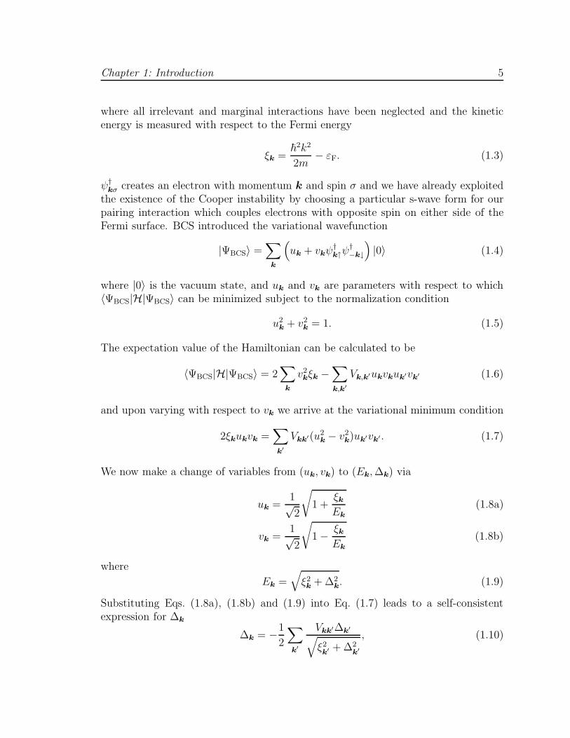
Substituting Eqs. (1.8a), (1.8b) and (1.9) into Eq. (1.7) leads to a self-consistentexpression for ∆k
∆k = −1
2
∑
k′
Vkk′∆k′√ξ2k′ + ∆2
k′
, (1.10)

Chapter 1: Introduction 6
which is known as the BCS gap equation. Eq. (1.9) certainly gives the impressionthat ∆k should be associated with an energy gap, but before we present a solution toEq. (1.10) we will confirm that this is indeed the case.
Let us return to our original reduced BCS Hamiltonian, and define new fermionoperators
ψ†−k↓ = −v†
kγk0 + ukγ†k1 (1.11a)
ψk↑ = u†kγk0 + vkγ
†k1 (1.11b)
with uk and vk taking the values in Eq. (1.8a) and (1.8b). We have changed from thespin indices (↑, ↓) to the generic labels (0, 1) to indicate that γk,0 can either destroyan electron with momentum k and spin ↑ or create one with momentum −k and spin↓. The net result of such an operation is to decrease the total momentum by k andthe total z-component of the spin by !/2.
The values of uk and vk which lead to a minimum variational energy also diago-nalize our Hamiltonian and we are left with
H = E0 +∑
k
Ek(γ†k0γk0 + γ†k1γk1) (1.12)
where E0 is a constant equal to the energy of the normal state plus the condensationenergy. In this form, it is readily apparent that the γkj describe the elementaryquasiparticle excitations of the system with energy Ek =
√ξ2k + ∆2
k and thus ∆k canbe identified as the superconducting energy gap; the energy needed to break a singleCooper pair.
Now returning to Eq. (1.10) we take the simplest possible form for the pairinginteraction
Vkk′ =
−V ; |ξk|, |ξk′| ≤ !ωD
0 ; otherwise(1.13)
where V > 0, immediately leading to
∆k =
0 ; |ξk| > !ωD
∆ ; |ξk| < !ωD(1.14)
with ωD the phonon Debye frequency and ∆ a constant. This form leads to a muchsimplified gap equation given by
1 =V
2
∑
k
1√ξ2k + ∆2
. (1.15)
Converting the sum over k into an integral over energy using the normal density of

Chapter 1: Introduction 7
states N(ξ) we find
1
N(0)V=
!ωD∫
0
dξ√ξ2 + ∆2
= sinh−1
(!ωD
∆
)(1.16)
where we have replaced N(ξ) ≈ N(0), the density of states at the Fermi energy sincewe are only interested in a small interval of width !ωD * εF. We find a solution onlyif V > 0 and in the weak coupling regime where N(0)V * 1 (which is almost alwaysjustified) we finally arrive at the solution
∆ + 2!ωDe−1/N(0)V . (1.17)
This result, valid at T = 0 has two immediately striking properties. The first is thata solution exists for an arbitrarily small value of the attractive interaction −V ; theFermi liquid is always unstable to pairing. The second is that ∆ is a non-analyticfunction of the strength of the coupling and thus no perturbative methods at weakcoupling could ever reproduce Eq. (1.17).
Finite temperature
The method just presented for the derivation of the gap equation can be straight-forwardly generalized to T > 0. The major modification is that at finite tempera-ture, quasiparticles above the superconducting ground state will be thermally excited.However, it turns out that they can be approximated as a gas of non-interactingparticles and the only modification will be that the gap ∆ acquires a temperaturedependence. The finite temperature self-consistency equation which corresponds toEq. (1.16) is now given by
1
N(0)V=
!ωD∫
0
dξ√ξ2 + ∆2
[1− 2f
(√ξ2 + ∆2
)](1.18)
where f(x) is the Fermi function
f(x) =1
ex/kBT + 1. (1.19)
It is easy to see that in the limit T → 0 this reduces to our previous result. Thetransition temperature Tc is defined as the temperature at which the gap identicallyvanishes and we have
1 = N(0)V
!ωD∫
0
dξ
ξtanh
ξ
2kBTc. (1.20)

Chapter 1: Introduction 8
For kBTc * !ωD we find
1 = N(0)V ln1.14!ωD
kBTc(1.21)
orkBTc = 1.14!ωDe−1/N(0)V . (1.22)
Again we see that for any non-zero pairing interaction this equation has a solutionand thus there will be a continuous phase transition to a superconducting state asthe temperature is lowered through Tc.
The methods we have used can be extended to calculate various thermodynamicquantities which can be compared with experiments using the known value of theDebye frequency with appreciable success. In this way, the value of N(0)V can beextracted and its value is always found to be small, justifying our weak couplingapproximation. We will eventually return to Eqs. (1.18) and Eq. (1.21) in the contextof the pair-breaking transition but for now we conclude this section with the commentthat although BCS theory works remarkably well, its key assumption is the lack ofany spatial dependence of the gap ∆. To address the theory of superconductors inconstrained geometries or in the presence of additional perturbations we will haveto appeal to macroscopic Ginzburg-Landau, theory which directly describes a slowlyvarying superconducting order parameter.
1.2 Fluctuations in low dimensional superconduc-tors
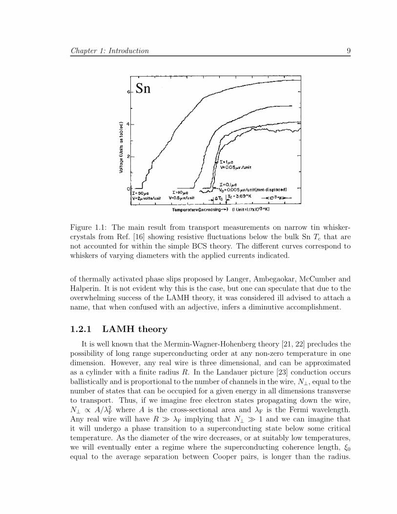
In 1968, Webb and Warburton performed a remarkable transport experiment onthin whisker-crystal Sn wires [16] with the result shown in Fig. 1.1. The tin whiskershad diameters between 40 and 400 µm and they noticed that for the thinnest wires,resistive fluctuations leading to a finite voltage persisted below the bulk critical tem-perature for tin. This strongly departed from any mean field estimates using themaximum supercurrent [17].
The understanding of this behavior, which is specific to quasi-one dimensionalsuperconductors followed rapidly thereafter and is composed of three parts. Thefirst was Little’s qualitative introduction of thermally activated phase slips [18]; ajump in the phase of the superconducting order parameter by ±2π, equivalent to avortex tunneling across the system. Next came the Ginzburg-Landau (GL) theory ofLanger and Ambegaokar [19] for the free energy barrier height of a phase slip eventwhich qualitatively reproduced the most important features of Webb and Warburton’sexperiments. The story concludes with the time-dependent Ginzburg-Landau theoryof McCumber and Halperin [20] who correctly computed the rate at which theseresistive fluctuations occur, and led to full quantitative agreement. Little’s initial isnot prepended to the acronym LAMH which is used as the moniker for the theory
Chapter 1: Introduction 9
Sn
Figure 1.1: The main result from transport measurements on narrow tin whisker-crystals from Ref. [16] showing resistive fluctuations below the bulk Sn Tc that arenot accounted for within the simple BCS theory. The different curves correspond towhiskers of varying diameters with the applied currents indicated.
of thermally activated phase slips proposed by Langer, Ambegaokar, McCumber andHalperin. It is not evident why this is the case, but one can speculate that due to theoverwhelming success of the LAMH theory, it was considered ill advised to attach aname, that when confused with an adjective, infers a diminutive accomplishment.
1.2.1 LAMH theory
It is well known that the Mermin-Wagner-Hohenberg theory [21, 22] precludes thepossibility of long range superconducting order at any non-zero temperature in onedimension. However, any real wire is three dimensional, and can be approximatedas a cylinder with a finite radius R. In the Landauer picture [23] conduction occursballistically and is proportional to the number of channels in the wire, N⊥, equal to thenumber of states that can be occupied for a given energy in all dimensions transverseto transport. Thus, if we imagine free electron states propagating down the wire,N⊥ ∝ A/λ2
F where A is the cross-sectional area and λF is the Fermi wavelength.Any real wire will have R . λF implying that N⊥ . 1 and we can imagine thatit will undergo a phase transition to a superconducting state below some criticaltemperature. As the diameter of the wire decreases, or at suitably low temperatures,we will eventually enter a regime where the superconducting coherence length, ξ0equal to the average separation between Cooper pairs, is longer than the radius.

Chapter 1: Introduction 10
This condition defines the quasi-one dimensional limit, as paired electrons necessarilyexperience the finiteness of the transverse dimension while unpaired electrons do not.
The presence of resistive fluctuations in a narrow wire implies that there are spatialvariations in the magnitude of the superconducting order parameter along its length.In the presence of such inhomogeneities, the BCS theory is not entirely appropriateand we instead appeal to the simple Ginzburg-Landau theory of the superconductingstate [6]. In the quasi-one dimensional case, this phenomenological theory assumesthat the free energy of a superconductor of length L and cross-sectional area A = πR2
can be written in the form
F = A
L∫
0
dx
[|∇Ψ|2 + α|Ψ(x)|2 +
β
2|Ψ(x)|4
](1.23)
where α, β and are arbitrary parameters for the chosen normalization of the orderparameter. Ψ(x) = ∆(x)eiϕ(x) is the complex superconducting order parameter thatis assumed to vary slowly along the x direction and be essentially constant in thetransverse directions. The phenomenological theory can actually be rigorously derivedas a limiting case of the microscopic theory in the spatially inhomogeneous regime[24].
The stationary condition δF/δΨ∗ = 0 leads to the Ginzburg-Landau differentialequation
−∇2Ψ + αΨ + β|Ψ|2Ψ = 0 (1.24)
for suitable boundary conditions. Introducing the magnetic vector potential A throughthe standard replacement ∇ → ∇ − (ie∗/!c)A the constant current solution toEq. (1.24) is a helix described by
Ψ(x) =
√α− k2
βeiϕ(x) (1.25)
where ϕ(x) = kx and the pitch is 2π/k. The allowed wavevectors k = (2π/L)n wheren is an integer are fixed by requiring that the order parameter be single valued forperiodic boundary conditions, ϕ(x+L) = ϕ(x)+2πn. This is equivalent to taking ourwire of radius R and length L and connecting it end-to-end to form a loop. Thus foreach integer n there exists a helical solution given by Eq. (1.25) which is an isolatedsaddle-point of Eq. (1.23). A continuous path in function space connecting two suchsolutions must overcome a free energy barrier.
In this multiply connected geometry, the requirement for a dissipationless currentis the familiar flux quantization condition
∮∇ϕ · d! = 2nπ. (1.26)

Chapter 1: Introduction 11
However, for a straight finite wire with an imposed current, the potential differencebetween the two ends is related to the rate of change in time of the total phasedifference via the Josephson relation [25]
d∆ϕ
dt=
2eV
!, (1.27)
where ∆ϕ = ϕ(L) − ϕ(0). In this configuration, a supercurrent, defined by V = 0requires a constant value for the phase difference, or at least a fluctuating alternatingcurrent (ac) value which oscillates about some mean. The measurement of a finitevoltage which is constant in time implies that the phase difference ∆ϕ must be in-creasing linearly with time. This can be understood by imagining that the helicalsolution described above is fixed at one end of the wire while it is continually woundat the other end around the x axis. Re-expressing this winding phase in terms of thesuperfluid velocity vs, the Josephson relation, Eq. (1.27) can be written as
dvs
dt=
eE
m. (1.28)
The tighter the order parameter is wound, the greater the cost in kinetic energycoming from an increasing superfluid velocity vs contributing to Eq. (1.23). Thus,there is a critical velocity vc related to the critical current Jc where the entire pictureof a uniform solution breaks down.
Little [18] arrived at the solution to this problem by suggesting that the steady-state could be maintained in the presence of a finite voltage, provided that the orderparameter was unwound by phase slips of 2π occurring at the exact rate needed tosatisfy Josephson’s relation. The important point is that since the order parametermust vary continuously, if its ends are held fixed, a phase slip event can only occur at alocation along the x-axis where the magnitude of the order parameter is spontaneouslysuppressed to zero. As shown in Fig. 1.2 with ∆ϕ going from 12π to 10π, phasecoherence is broken in some localized region along the wire, and a single loop isunwound before coherence is reestablished. Phase changes of more than 2π are aresult of a sequence or cascade of single slips.
A single phase slip is thus a thermally induced activated resistive fluctuation thatoccurs at a random position in the wire. With this picture in mind, Langer andAmbegaokar (LA) [19] set out to determine the height of the minimum free energybarrier along the path in function space that connects two saddle point solutions ofEq. (1.23) corresponding to uniform solutions with different numbers of turns. Theyderived the physically appealing result that the free energy barrier is proportional tothe condensation energy in one correlation length of the conductor
∆F =8√
2
3
H2c (T )
8πAξ(T ) (1.29)

Chapter 1: Introduction 12
x
ImΨ
ReΨ
Figure 1.2: A schematic snapshot of the order parameter Ψ at some fixed time fora current carrying state at constant voltage. The total phase difference between thetwo ends changes from 12π in the top panel to 10π in the bottom panel as a result ofa single phase slip event pictured at center.
where H2c (T )/8π is the superconducting condensation energy per unit volume intro-
duced previously, A is the cross-sectional area of the wire and ξ(T ) is the Ginzburg-Landau correlation length at temperature T . McCumber [26] showed that in the inthe absence of an applied current, phase slips of ±2π will occur with equal probabil-ity. In the presence of small current, the arguments above require that −2π phaseslips occur at rate of 2eV/h per second greater than +2π slips. This is related to thedifferent electrical work corresponding to plus and minus jumps
δF ≡ ∆F+ −∆F−
=h
2eI (1.30)
where I is the applied current. In order to determine the rate of change of the phasedifference between the two ends, an attempt frequency Ω must also be calculated.Langer and Ambegaokar essentially guessed that this was the temperature indepen-
Chapter 1: Introduction 13
dent quantity
Ω =NAL
τe(1.31)
where N is the density of conduction electrons in the wire and τe ≈ 10−12 s is thetypical elastic scattering time of electrons in the normal state. The time rate of phasechange between the ends of the wire is thus given by
d∆ϕ
dt= Ωe−∆F/kBT
(eδF/2kBT − e−δF/2kBT
)
= 2Ωe−∆F/kBT sinhδF
2kBT(1.32)
which when combined with Eq. (1.30) and inserted into the Josephson relation,Eq. (1.27) leads to the voltage
VLAMH =!Ω
ee−∆F/kBT sinh
hI
4ekBT. (1.33)
In the limit of small currents we assume there is a linear resistance coming fromOhm’s law and thus
RLAMH =π!2Ω
2e2kBTe−∆F/kBT . (1.34)
McCumber and Halperin (MH) realized that although the LA result for the size ofthe free energy barrier was correct, they had drastically overestimated (by a factor ofalmost 1010!) the rate at which phase slips occur. They reformulated the problem interms of the time dependent Ginzburg-Landau theory and discovered that althoughthe basic structure of the MH form for Ω is correct, when derived properly it istemperature dependent and equal to
Ω(T ) =L
ξ(T )
√∆F
kBT
1
τGL(T )(1.35)
where
τGL(T ) =π!
8kB(Tc − T )(1.36)
is the Ginzburg-Landau relaxation time. Instead of being equal to the number ofelectrons per unit electron relaxation time, it is equal to the number of statisticallyindependent sub-regions of the wire where a phase slip process could occur per unitsuperconducting relaxation time.
Due to the use of the GL free energy, this result should work only arbitrarily closeto Tc, but when adding a normal resistive channel (RN) in parallel, such that thetotal resistance is given by
R =
(1
RN+
1
RLAMH
)−1
, (1.37)

Chapter 1: Introduction 14
excellent agreement was found over six orders of magnitude for micron diameter Snwhiskers. It would be almost thirty years before technological advances in fabricationtechniques had improved enough to reduce the diameters by a factor of one thousand,pushing the limit of the LAMH theory and entering a truly quantum regime.
1.3 Ultra narrow wires
The self grown Sn-whiskers of the original Webb and Warburton experiment haddiameters between 40 and 400 µm and their resistive properties were well describedby the LAMH theory introduced in the previous section. As the diameter of a wire isreduced, there are two important changes that need to be considered. The first is thewell known volume to surface area ratio, and thus surface effects which are somewhatpoorly understood will begin to affect bulk behavior. The second is more subtleand is related to the increased effects of coupling with an external environment. Inthe presence of such dissipation, a small system can undergo a quantum localizationtransition, as is observed in small Josephson junctions [27].
1.3.1 Evidence for quantum phase slips
In the early 1990s, step edge electron beam lithography techniques were used tocreate narrow indium strips with diameters between 40 and 100 nm. When transportmeasurements were performed, there appeared to be significant deviations from theLAMH resistance at low temperatures resulting in a persisting resistance manifestas a “foot” raised upwards from the expected exponentially decreasing behavior [28,29]. It was proposed that this was due to the onset of quantum phase slips at lowtemperatures occurring via the macroscopic tunneling mechanism of Caldeira andLeggett [30]. These ideas were vigorously pursued [31, 32, 33, 34] leading to a host oftheories which did not necessarily agree on the observability of quantum phase slipsin experiments. One of the most interesting results was a upper bound on the wirediameter of approximately 10 nm above which quantum phase slips would be stronglysuppressed [32] as their rate ΩQPS ∼ exp(−N⊥) where N⊥ is the number of transversechannels in the wire discussed above. This upper bound of ten nanometers was fartoo narrow for step edge lithography techniques and it would take the invention ofnovel nanofabrication methods to fully address these issues.
1.3.2 Suspended molecular templating
Wires with truly nanoscale dimensions were not studied until the introduction ofa novel and pioneering nanofabrication technique known as suspended molecular tem-plating in early 2000 [35]. This remarkable process can be used to manufacture wireswith lengths between 100 and 200 nm with diameters less than 10 nm. The key feature

Chapter 1: Introduction 15
100nm
MoGe
Figure 1.3: A diagram courtesy of Ref. [36] of an ultra-thin wire fabricated via sus-pended molecular templating which results in a single nanowire held up over a trenchby a bridge consisting of a single carbon nanotube. The inset shows a scanningelectron microscopy image of a MoGe nanowire with a diameter of approximately10 nm.
is the top down approach that uses a long narrow molecule such as a carbon nanotubeor DNA as a backbone on top of which the wire is deposited. The fabrication processbegins by etching a trench in a substrate formed from a silicon wafer using electronbeam lithography. The backbone molecules are then placed in solution and depositedover the substrate. They are allowed to settle, and at high concentrations some willend up resting over the trench. The entire surface of the substrate is then sputtercoated with several nanometers of a metal like Nb or alloy such as MoGe. The resultis that a thin uniform layer of the deposited material is suspended over the trench bythe backbone molecule. It can be located via scanning electron microscopy (SEM)and then isolated with a mask that is also used to pattern electrodes that will be usedfor transport measurements. A schematic view of the final system is shown in Fig. 1.3with an inset showing an actual SEM image of a MoGe nanowire. A huge advantageof the SMT technique, in addition to allowing for the fabrication of ultra narrow wires,is that it allows for a large number of wires with varying diameters to be quickly andeasily made. Fig. 1.4 reproduces resistance versus temperature measurements fromRef. [37] for five wires ranging in diameter from 10.5 nm to 6.8 nm. The results showtwo exponential dips in the resistance for each wire. The first at high temperatures,corresponds to the large two dimensional leads going superconducting while the lowertemperature drop is due to the actual wire undergoing a phase transition. The tem-perature at which the wire goes superconducting is strongly dependent on its diameterwith thinner wires being pushed to lower temperatures. This is consistent with our

Chapter 1: Introduction 16
Figure 1.4: Experimental transport measurements on MoGe nanowires from Ref. [37]showing excellent agreement with the LAMH theory of thermally activated phaseslips (TAPS) for resistances down to approximately 0.5 Ω. The diameters of wiresMG1 to MG4 are 10.4, 10.0, 9.4 and 6.8 nm respectively.
expectations as discussed at the beginning of this section. Superb agreement with theLAMH theory is found for resistances down to 0.5 Ω using Eq. (1.34) with the bulkcritical temperature Tc and the zero temperature coherence length ξ(0) used as fittingparameters. At resistances below this value, or for thinner wires, there appears to bea growing experimental consensus that there is a non-monotonicity in the resistanceand deviations from the theory of purely thermally activated phase slips. The wiresseem to be entering a regime where resistive fluctuations coming from other effects,possibly including Coulomb blockade and quantum phase slips can either postponeor completely destroy the superconducting transition [35, 38, 39, 40]. This behaviorcan be seen by measuring the resistance of thinner and thinner wires as a function oftemperature leading to a separation between superconducting and metallic transportall the way down to the lowest temperatures as seen in Fig. 1.5. If superconductivityis indeed being destroyed as the temperature is reduced to zero by quantum and notthermal fluctuations upon tuning some parameter related to the size of the transversedimension, then such a transition is by definition a superconductor-metal quantumphase transition (SMT).
Chapter 1: Introduction 17
thickest
thinestthinnest
Figure 1.5: Experimental transport measurements on MoGe nanowires from Ref. [36]showing a distinct difference between thick superconducting and thin metallic orresistive wires as the temperature is reduced. At zero temperature, a quantum criticalpoint would separate the superconducting and metallic phase, with the transitionbetween them being described by a quantum superconductor-metal transition (SMT).
1.4 Pair-breaking theory
We have just seen a plot of the resistance versus temperature for a set of ultra-narrow MoGe wires with varying diameters (Fig. 1.5). As temperature was reducedthe thicker wires all underwent a superconducting transition but it appeared thatthere was some critical wire diameter, below which no such transition occurred. In-stead, the thinnest wires displayed metallic or resistive behavior down to the lowesttemperatures measured and some even hinted at non-monotonic behavior in T . Weproposed an explanation for these observations in terms of a quantum phase tran-sition between a superconducting and metallic state, a SMT, that appeared to betuned by the radius of the wire. The temperature-radius phase diagram would takethe form of the schematic one depicted later in Fig. 1.10 where the choice of symbolfor the tuning parameter seems particularly apt.
In our presentation of the BCS theory of conventional superconductivity we de-

Chapter 1: Introduction 18
rived an explicit equation for the transition temperature
kBTc = 1.14!ωDe−1/N(0)V (1.38)
where ωD was the phonon Debye frequency, N(0) the density of states at the Fermienergy and V the pairing strength. We argued that this expression guarantees thatthere will always be a superconducting state below some temperature for an arbitrarilysmall value of V . Our conclusions about the complete destruction of superconduc-tivity in ultra-thin wires therefore seems to be at odds with a Nobel prize winningtheory, an uncomfortable position to linger in. Luckily, this apparent contradictionwas resolved some time ago by Abrikosov and Gor’kov (AG) [41] when they studiedthe suppression of Tc in superconducting alloys with paramagnetic impurities. Theydiscovered that in the presence of a perturbation which makes it more difficult to formCooper pairs, a pair-breaking interaction, Eq. (1.38) gets modified and some criticalpairing strength is needed to form the superconducting state. The AG theory hassince been generalized to many different sources of physical pair-breaking interactionsand we will introduce the important features of their arguments as well as discusssome modern experimental realizations of the pair-breaking transition.
1.4.1 Magnetic fields and impurities
The most important observation that led to the pair-breaking theory was that thetransition temperature of a clean superconductor is almost completely unchanged bythe addition of a moderate concentration of non-magnetic impurities. This behav-ior is fully explained by Anderson’s theorem [42] which states that although smallconcentrations of disorder will lead to some local impurity states, the system is stillnearly homogeneous at lengths on the order of the BCS coherence length ξ0, and thusCooper pairs are not significantly affected. The Anderson theorem breaks down in thepresence of magnetic impurities as a Cooper pair is composed of two electrons whichare time reversed partners (opposite momentum and spin). Thus any perturbationwhich is odd under time reversal will act differently on the two paired electrons andlead to a finite probability of completely disassociating the pair. If the strength ofthe pair-breaking is large, ξ0 can be reduced enough to completely destroy the phasecoherent superconducting state.
The only restriction on a pair-breaking perturbation is that it must act oppo-sitely on the two members of a Cooper pair. This condition is satisfied in a smallor dirty superconductor placed in a suitably strong magnetic field. In addition, a re-stricted geometry leading to sufficient surface scattering or non-magnetic impuritiesproviding body scattering and diffusive behavior are required to ensure that indi-vidual pair-breaking events are rapid and uncorrelated and that the electrons canexplore their full phase space leading to so called ergodic behavior. A magnetic fieldcan be incorporated into the single electron Hamiltonian in the usual way leading toa term of the form p · A + A · p where p is the momentum and A is the magnetic

Chapter 1: Introduction 19
vector potential. This term is clearly odd under time reversal, changing sign whenp → −p. The contribution of a magnetic impurity as described by the AG theory ismore complicated, and will couple to electrons via a super exchange mechanism
Hex = J(|x− x′|)S(x) · σ(x′) (1.39)
where S(x) is the impurity spin located at position x and σ(x′) is the electron spinat x′. Since a Cooper pair is made up of two paired electrons, one with spin σ andthe other with spin −σ such an exchange term will cause spin flip scattering with anopposite orientation for each member.
Abrikosov and Gor’kov studied the latter case within the diagrammatic Greenfunction formalism using the Born approximation for the scattering of an electron offan impurity atom. We will spare the reader from a presentation of their methodsand instead quote some of the important results from de Genne’s treatment [15]using the linearized Ginzburg-Landau equations in the presence of a constant pairpotential which will be sufficient for our purposes. After some preliminary algebraand simplifications, the final discussion can be framed in terms of the time reversalHeisenberg operator K(t) which acts on the single electron wave functions of thenormal metal.
We begin with the usual local electron Hamiltonian
He =∑
σ
∫ddx
ψ†σ(x)
[1
2m
(p−
e
cA)2− εF
]ψσ(x) +
∑
σ,σ′
ψ†σ(x)Uσσ′(x)ψσ′(x)
− V∑
σ,σ′
ψ†σ(x)ψ†
σ′(x)ψσ(x)ψσ′(x)
(1.40)
where ψ†σ(x) creates an electron at site x with spin σ and Uσσ′(x) is a static, local
spin-dependent interaction. This Hamiltonian includes both types of pair-breakinginteractions discussed above and the self-consistency equation for the superconductinggap ∆ is given by
∆ =V
2
∑
σ,σ′
εσσ′〈ψσ(x)ψσ′(x)〉 (1.41)
where 〈· · · 〉 indicates an average with respect to He and εσσ′ is a fully antisymmetrictensor.
The equations of motion for ψ† and ψ can be linearized, and diagonalizing theHamiltonian by introducing Bogoliubuv quasiparticles we arrive at a modified versionof Eq. (1.41) (after some considerable algebra)
∆(x) =
∫ddx′Φ(x, x′)∆(x′) (1.42)

Chapter 1: Introduction 20
to lowest order where
Φ(x, x′) =∑
ωn
∫dξ
∫dξ′
kBTV N(0)V(ξ − i!ωn)(ξ′ + i!ωn)
g(x, x′, ξ − ξ′) (1.43)
with V the volume of the system, V the BCS pairing interaction, N(0) the densityof states at the Fermi level and ωn = (2n + 1)πkBT/! an odd electron Matsubarafrequency. The function g is defined by
g(x, x′, ε) =∑
m
〈φ∗n(x)φ∗m(x)φm(x′)φn(x′)〉 δ(ξm − ξn − ε) (1.44)
where φm are the normal electron eigenstates of He. Eq. (1.43) should remind thereader of Eq. (1.18) and a key simplification will come by recognizing that the timereversal operator has been essentially defined to lead to the conjugation of thesestates, i.e.
Kφm(x) = φ∗m(x). (1.45)
Using this fact we can rewrite Eq. (1.43) in terms of g, the power spectrum of theoperator K
!
N(0)V=∑
ωn
∫dξ
∫dξ′
kBT
(ξ − i!ωn)(ξ′ + i!ωn)g
(ξ − ξ′
!
)(1.46)
where
g(ω) =
∫dt
2π〈K†(0)K(t)〉e−iωt. (1.47)
The first thing to note is that in the absence of any pair-breaking perturbations
〈K†(0)K (t)〉 = 1 (1.48)
and g(ω) = δ(ω). Eq. (1.46) thus reduces exactly to Eq. (1.18) in BCS theory. Inthe presence of a pair-breaking interaction, the ergodicity condition discussed earlieris equivalent to requiring that
〈K†(0)K (t)〉 ∼ e−t/τK (1.49)
as t → ∞ where τK is the time required to sufficiently randomize the phase ofthe two electrons composing a single Cooper pair; the spin-flip scattering time. Acorresponding energy scale,
!α =!
2τK, (1.50)
can be interpreted as the depairing energy or splitting between the two time-reversedelectrons of a Cooper pair, averaged over the time required to completely uncorre-lated their phases. This interpretation allows one to generalize the pair-breaking

Chapter 1: Introduction 21
theory presented here to large variety of physical situations provided the destructionof superconductivity occurs via a second order phase transition [15].
Substituting Eq. (1.49) in Eq. (1.47) we find
g(ω) =1
π
τK1 + ω2τ 2
K
(1.51)
which can be inserted into into Eq. (1.46), and performing the two energy integralswe arrive at
1
N(0)V=
kBT
!
∑
ωn
2π
2|ωn| + τ−1K
. (1.52)
The sum is divergent as a result of the fact that we have forgotten to enforce theBCS constraint in Eq. (1.13). Taking this into account, and adding and subtracting∑
ωn(2|ωn|)−1 the equation for the critical temperature is given by
1
N(0)V=
[
ln
(1.14!ωD
kBT
)+
2πkBT
!
∑
ωn
(1
2|ωn| + τ−1K
−1
2|ωn|
)]
(1.53)
where we have used Eq. (1.38). The sum can now be performed and yields the finalAG result for the mean field pair-breaking phase boundary
ln
(T
Tc0
)= ψ
(1
2
)− ψ
(1
2+
!α
2πkBT
)(1.54)
where ψ(x) is the polygamma function, kBTc0 = 1.14!ωDe−1/N(0)V is the BCS tran-sition temperature in the absence of any pair-breaking perturbations and α is thepair-breaking frequency defined in Eq. (1.50). Eq. (1.54) is the main result of thissection and shows that by perturbing a conventional superconductor with a suitablystrong interaction that breaks time reversal symmetry, it is possible to completelydestroy the superconducting state at finite temperature as shown in Fig. 1.6. Math-ematically, this is equivalent to the observation that for large enough α, Eq. (1.54)has no non-zero solution at finite temperature.
1.4.2 Experimental manifestations
We have presented a derivation of the relationship between the pair-breaking fre-quency α and the temperature at which superconductivity is destroyed for the partic-ular case of a superconductor with paramagnetic impurities. However, we argued thatthe result is much more general and can be applied to any perturbation which breakstime reversal symmetry. We now introduce three experimentally tunable sources ofpair-breaking which are of considerable interest.

Chapter 1: Introduction 22
0.0 0.2 0.4 0.6 0.8 1.0 1.2 1.4
hα/kBTc0
0.0
0.2
0.4
0.6
0.8
1.0
1.2
T/T
c0
Figure 1.6: The Abrikosov-Gor’kov pair-breaking phase diagram [41] with the phaseboundary given by Eq. (1.54). The superconducting phase is shaded, and for a suit-ably large α the ordered phase is completely destroyed for all finite temperatures.
Radius tuned nanowire
A possible superconductor-metal transition in ultra-narrow MoGe wires was dis-cussed at the beginning of this section inferred from an examination of Fig. 1.5. Atfirst glance, it would appear to be driven by a source of pair-breaking related to thediameter of the wire, however this could be an example of correlation not implyingcausation. Recent experiments have provided some evidence [37] that there may bemagnetic impurities sitting on the surface of nanowires made using the SMT tech-nique. Any impurity at the surface would be much less effectively screened, and onecould imagine a BCS coupling V (ρ) which depends on the radial coordinate of thewire. In this picture, V (ρ) would change sign from negative (attractive) to positive(repulsive) as ρ changes from ρ = 0 to ρ = R where R is the diameter of the wire.This behavior is schematically outlined in Fig. 1.7. For the thickest wires, R > ξ0 andthe mean field solution to the BCS equations will lead to the wire being describedby a superconducting core surrounded by a cylindrical metallic envelope. A similarpicture was recently put forward to describe the SMT in two dimensions by imag-ining superconducting grains embedded into a film with a pairing interaction whichdepended on the distance from the center of the islands [43]. In the nanowire case, asone reduces the transverse dimension, there will be a critical radius, R ≈ ξ0, where
Chapter 1: Introduction 23
V < 0
V > 0
Figure 1.7: A schematic cross-section of a metallic wire where magnetic impuritieson the surface are poorly screened leading to a change in sign of the BCS pairinginteraction as one moves from the center, |Ψ| 3= 0 to the edge, |Ψ| + 0 where Ψ(ρ) isthe superconducting order parameter. Below some temperature, the wire would becomposed of a superconducting core with a normal resistive sheath.
the superconducting core will vanish and the wire will enter a metallic state. This isa rather physically appealing picture as it is suitable for the destruction of supercon-ductivity in a wire that is only weakly disordered in the bulk and is well suited totheoretical models.
Magnetic field tuned nanowire
It is clearly impossible to systematically reduce the diameter of a single wire whilemeasuring its transport properties and thus other more systematic examples of a SMTwould be beneficial. The most obvious candidate is a transition that can be observedin a single wire by increasing the strength of a magnetic field oriented parallel to itslong axis. This experiment has been performed by Rogachev, Bollinger and Bezryadin[44] on individual Nb nanowires with the most important result shown in Fig. 1.8. Therightmost curve is in zero magnetic field and shows a superconducting transition thatis well described by LAMH theory (solid line). As the strength of the parallel magneticfield is increased, the transition appears at lower and lower temperatures with theexpectation that for suitably strong fields it will vanish all together and the wire willexhibit metallic behavior; a quantum SMT. To completely destroy superconductivity,pair-breaking events must be uncorrelated over long time scales and a theoreticaldescription would require diffusive electrons or suitably strong boundary scattering.

Chapter 1: Introduction 24
Figure 1.8: Resistance versus temperature for a Nb nanowire with a diameter of 8nmand length L = 120nm in a parallel magnetic field with strength ranging from 0 T(right curve) to 11 T (left curve). The symbols are data points while the lines are fitsto LAMH theory using Tc and ξ0 as free parameters.
Magnetic flux tuned cylinder
A final experimental example which is relatively well understood is the destructionof superconductivity in a multiply connected metallic cylinder with a nearly half-integer flux quantum trapped in its interior. Liu et al. have fabricated ultra-thindoubly connected metallic cylinders by coating quartz poles with aluminum [45].The Al coating is thin enough to be considerably smaller than the penetration depthin the presence of a magnetic field oriented parallel to the long axis of the cylinder.Below some transition temperature the doubly connected cylinder will exhibit thewell known phenomena of flux quantization in an external field as a result of globalphase coherence and a circulating supercurrent around the cylinder. Because of thenarrow walls, the superfluid velocity vs should be constant in the aluminum and for agiven value of the external magnetic flux Φ =
∫H · dS through the cylinder we find
vs =!
m∗R
(n−
Φ
Φ0
)(1.55)
where R is the radius, Φ0 = h/2e is the flux quantum and m∗ is twice the electronmass. The integer n will adjust to minimize vs for a given field strength and thisis known to lead to Little-Parks oscillations in the critical temperature for large R[46]. However, if the radius of the wire is reduced until it is on the order of the

Chapter 1: Introduction 25
Figure 1.9: The superconductor-normal phase diagram for a 150 nm long ultra-thinwalled aluminum cylinder as a function of the magnetic flux trapped inside, measuredin units of the flux quantum Φ0 = h/2e from Ref. [45].
superconducting coherence length, the ordered state can completely disappear. FromEq. (1.55), the superfluid velocity will reach a maximum whenever Φ/Φ0 is equalto a half-integer. Due to the small sample volume, the condensation energy cannotovercome the drastic increase in kinetic energy due to vs and superconductivity will nolonger be energetically possible. This completely destructive quantum size effect wasfirst observed in Ref. [45] and is highlighted in the phase diagram shown in Fig. 1.9.We observe a lobed structure showing finite temperature phase transitions betweena superconducting and normal state, as well as indicating the presence of a seriesof quantum critical points at field strengths corresponding to a half integer trappedflux. The transition is crucially dependent on the specific topology of the system andis therefore not directly amenable to a microscopic pair-breaking description.
In this section we have presented three experimental examples of a quantum phasetransition between a superconductor and a metallic state tuned by a non-thermalparameter. The quantum SMT is a single example of a broader class of transitionsdriven by quantum fluctuations at zero temperature. The complex interplay betweenthermal and quantum fluctuations will lead to a host of novel and interesting phasetransitions and crossovers which we now address.

Chapter 1: Introduction 26
1.5 Quantum phase transitions
In the previous section we were led by an analysis of experimental results to theconcept of a phase transition between a superconductor and a metal occurring at zerotemperature, driven by quantum and not thermal fluctuations in a ultra-narrow wireor cylinder. This is just one example of a fascinating type of phase transition wherethe dynamic and static critical behavior are inexorably intertwined. The couplingbetween thermodynamics and dynamics at all length scales at T = 0 can have drasticand non-trivial effects throughout the finite temperature phase diagram and in thissection we present the basic ingredients that will be necessary to motivate the resultsin the remainder of the thesis. The theory of quantum phase transitions and crossovershas been developing over the last thirty years with its official “coming out” party oftenattributed to Hertz [47]. As a result, many excellent books [48], lectures [49, 50] andcolloquia [51] have been written on the subject; with the author having a conspicuouspreference for Ref. [48].
We begin with a brief review of classical phase transitions and the scaling hy-pothesis which will be useful for mapping quantum phase transitions to their classicalcounterparts in one additional dimension. After highlighting the properties of thezero temperature quantum critical point, a generalization to finite temperatures isprovided, where the finite size of the system in the imaginary time direction will leadto highly non-trivial crossover phenomena. We finally conclude with a discussion ofthe failings of the quantum to classical mapping and the necessity of taking a quantumfield theoretic perspective from the outset.
1.5.1 Landau theory
The theory of classical phase transitions is built around the existence of an orderparameter which is identically zero in a disordered phase and takes on a finite value inan ordered phase. It is usually related to an obvious macroscopic feature in a physicalsystem such as the magnetization near a ferromagnetic transition or the density ofCooper pairs near a superconducting transition. A phase transition can occur betweenthe ordered and disordered phases (where disorder here refers to a phase without longrange order, not to be confused with quenched randomness or defects) by tuning thetemperature of the system. The nature of the phase transition, either continuous(second order) or discontinuous (first order) is related to the continuity of the orderparameter across the critical point. One of the most common phase transitions whichoccurs in nature, the melting of ice to form water is first order, as the two phasescoexist at the critical point and a latent heat is released. We will be primarilyconcerned with the theory of continuous phase transitions, which do not have phasemixing and exhibit fluctuations of the order parameter at the critical point with bothdiverging length and time scales. Standard sources which include much more detailon these and other points include Refs. [52] and [53].

Chapter 1: Introduction 27
Landau theory assumes that the free energy of the system F is analytic in aspatially uniform order parameter m and can be written as a power series expansion
F = hm + rm2 + vm3 + um4 + · · · (1.56)
where all constants h, r, v and u are unknown, but usually some of their values canbe set to zero by symmetry. For example if the system we are attempting to describewith F is invariant under the transformation m → −m then we would necessarilyrequire that h = v = 0 and we will consider this case here. It is also assumed thatthe leading order temperature dependence is contained within r = r0(T − Tc) whereTc is the critical temperature at which the phase transition occurs. In the absence ofthe linear or cubic terms, the free energy can be trivially minimized with respect tovariations of the order parameter and it is clearly seen that for T > Tc or r > 0 theminimum will occur for m identically zero. For T < Tc, r < 0 and a non-zero solutionappears with m =
√−r/2u.
If we identify m as the magnetization of a ferromagnetic Ising model, then as thecritical point is approached from the ordered phase m ∼ |r|β where β = 1/2 is a meanfield critical exponent, with similar exponents existing for other macroscopic observ-ables. Thus Landau theory provides an experimentally verifiable prediction for theonset of order in any system invariant under the change of sign of its order parameteras the temperature is reduced. This is an example of the concept of universality,where macroscopic critical behavior is independent of any of the microscopic detailsof a given system. Universality is indeed observed in experiments, but it is not asstrong as the hyper-universality of Landau theory would predict. In reality, differentsystems can be grouped into various universality classes which depend on both thedimension of space d and the number of components (or symmetry) N of the orderparameter.
The main flaw in Landau theory is that it does not allow for any fluctuations of theorder parameter about its mean field value. It is known that lower dimensions or moreorder parameter components tend to produce larger fluctuations, and such systems arepoorly described by Landau theory. This observation leads naturally to the conceptof an upper critical dimension dUCD above which fluctuations can be neglected andthe simple Landau theory provides the correct leading order physical description ofcritical behavior. On the other end of the spectrum lies the lower critical dimensiondLCD where fluctuations are so strong that they completely destroy the possibility ofany ordered phase, and no finite phase transition can exist. If the dimension of thesystem of interest lies between the lower and upper critical dimension than a phasetransition will exist, but it will exhibit non-mean field critical behavior.
dUCD = 4 for all values of N , while dLCD = 1 for N = 1 and dLCD = 2 for N > 1.A more subtle phase transition exists in the special marginal case of d = 2 and N = 2known as the Kosterlitz-Thouless (KT) transition.

Chapter 1: Introduction 28
1.5.2 The scaling hypothesis
The failings of Landau theory can be overcome below the upper critical dimensionby generalizing the spatially independent order parameter m to a coarse grained fieldφ(x) which should not be thought of as a microscopic variable, but rather as anaverage of some quantity over a region of space. With this generalization, the simplefree energy in Eq. (1.56) now takes the form of the classical O(N) model, a functionalin d dimensions where
F [φa] =
∫ddx|∇φa(x)|2 + rφ2
a(x) +u
4![φ2
a(x)]2 − haφa(x)
(1.57)
and a = 1, . . . , N will allow us to consider any order parameter symmetry and we usethe usual short form notation
φ2a(x) ≡ φ2
1(x) + · · · + φ2N(x). (1.58)
There is an energy cost associated with spatial gradients of the order parameter, andwe have added a field ha conjugate to φa. The partition function is defined by thefunctional integral over φa(x)
Z =
∫Dφa e−F [φa]/kBT , (1.59)
and the study of the free energy functional, F is referred to as the Ginzburg-Landau(GL) or Ginzburg-Landau-Wilson (GLW) theory. The field φa has been defined suchthat its average value with respect to Z, 〈φa(x)〉 is the Landau order parameter ofthe previous subsection
m ≡1
Z
∫Dφa φa(x) e−F [φa]/kBT (1.60)
where in general for any observable O
〈O〉 =1
Z
∫Dφa O e−F [φa]/kBT . (1.61)
The free energy functional in Eq. (1.57) was introduced in order to allow for the studyof fluctuations of the order parameter. These are characterized by its correlationfunction (or propagator)
G(x) = 〈φa(x)φa(0)〉 (1.62)
which is expected to decay exponentially with separation in the disordered phase
G(x) ∼ e−|x|/ξ (1.63)
defining the correlation length ξ. As the ordered phase is approached, correlationsdiverge as
ξ ∼ |r − rc|−ν (1.64)

Chapter 1: Introduction 29
where rc is the critical coupling signaling the onset of a phase transition and ν isdefined as the correlation length critical exponent. The diverging correlation lengthhas profound implications for critical phenomena, as it will be the only length scaleaffecting physical observables as the critical point is approached.
The existence of a single length scale is the crucial observation of the scalinghypothesis. Suppose we rescale all lengths in the system by a positive number b,but adjust all external parameters (temperature, magnetic field, etc) so that thecorrelation length retains its original value. We have just described a single iterationof the renormalization group (RG) procedure, and due to the sole dependence onξ, all physical quantities must remain unchanged. To be precise, consider the freeenergy density f defined by
f = −kBT
VlnZ (1.65)
where V is the volume. Performing the process described above for the Gaussiantheory (u = 0) we find a homogeneity relation for the singular part of the free energydensity
fs(r, h) = b−dfs(rb1/ν , hbyh) (1.66)
where yh is another critical exponent and we have rescaled our coupling r = r/r0 andfield h = h/h0 in order to make them dimensionless. In Eq. (1.66), b is a dimensionlessscaling factor that we are free to choose, so let us pick b = r−ν , and we have
fs(r, h) = rdνΦf
(h
rνyh
)(1.67)
where Φf is a scaling function. Although the specific microscopic details of a givensystem are obfuscated in the scale factors r0 and h0, the functional form of Φf doesnot, it is universal. Similar relations can be derived for other observables by takingthe appropriate derivatives of fs(r, h) leading to various universal critical exponents,and the scaling relations between them. The scaling laws can be rigorously derivedwithin the framework of the renormalization group and all together lead to remarkableuniversal critical behavior due to the presence of a single diverging length scale, ξ.
1.5.3 Quantum statistical mechanics
The fundamental result of the existence of homogeneity relations is that the crit-ical exponents that describe the properties of observables as the phase transition isreached are universal; they are the same for a wide variety of different types of phasetransitions in different physical systems. They depend only on the universality class,a function of the dimension of space and the symmetry of the order parameter. Allmicroscopic details are unimportant near the phase transition as the presence of a di-verging length scale of fluctuations effectively averages over a larger and larger volumeof the system.

Chapter 1: Introduction 30
Up until this point we have been able to completely neglect dynamics, or the time-dependence of physical observables, for the simple reason that in classical statisticalmechanics the kinetic and potential parts of the Hamiltonian commute and we wereable to study an effective classical field theory in terms a free energy functional F . Ifwe were instead to begin from a description of our system in terms of some N -particleHamiltonian H(pi, qi), then the partition function would be written as an integralover all phase space variables qi, pi:
Z =1
N !hNd
∫ ∏
i
dqidpi e−βH(pi,qi)
=1
N !hNd
∫ ∏
i
dpie−βHkin(pi)
∫ ∏
i
dqie−βHpot(qi)
= ZkinZpot, (1.68)
where β = 1/kBT and h is Planck’s constant. As the kinetic part simply consists ofa product of simple Gaussian integrals it is singularity free, and it can be neglected,allowing us to study thermodynamic critical behavior using time independent theo-ries, such as the GLW theory above. The situation is clearly not so simple in thequantum mechanical case where the kinetic and potential parts of the Hamiltoniando not commute. This is equivalent to the fact that when computing Z classically, weonly need the Hamiltonian and not the equation of motion, but both factor into thequantum calculation. In other words, H alone does not fix the equation of motion,but we also need the Poisson brackets or commutation relations to determine theclassical oscillation frequencies, ω, which when multiplied by ! give the energy levelspacings. As a result, the partition function does not factorize and we are left withthe task of computing
Z = Tr e−βH. (1.69)
The expression for the quantum partition function can be very elegantly analyzedin the path-integral formulation of quantum mechanics due to Feynman with all thedetails provided in Ref. [54]. We first recall the usual time evolution operator ofordinary quantum mechanics
U(t) = e−iHt/! (1.70)
and note that it is equal to the expression we are tracing over in Eq. (1.69) if weevolve over imaginary instead of real time, i.e. t = −iβ!. Then writing the trace asa sum over states n
Z =∑
n
〈n|U(−iβ!)|n〉 (1.71)
we observe that the partition function is just the sum of imaginary time transitionamplitudes for the case where the system begins and returns to the same state |n〉after an imaginary time −iβ!. We are thus led to one of the fundamental conclusionsof quantum statistical mechanics:

Chapter 1: Introduction 31
Calculating the thermodynamics of a quantum system is equivalent to com-puting transition amplitudes for its evolution over an imaginary time in-terval set by the measurement temperature.
In the path integral formulation, the net transition amplitude between any twostates of the system can be found by summing the individual amplitudes over allpossible space-time trajectories which connect them. The key point is that althoughit is not possible to calculate the individual amplitudes over the full imaginary timeinterval, for an infinitesimal time interval they may be calculated in perturbationtheory to any desired accuracy. We imagine breaking up the full time interval intoM steps and can write
U(−iβ!) = e−βH
=(e−∆τH/!
)M
= [U(−i∆τ)]M (1.72)
where ∆τ is taken to be a microscopic real time interval such that ∆τ = !β/Mcorresponding to the imaginary time interval −i∆τ with M a large integer. Weproceed by inserting M complete sets of of intermediate states into our expression forthe partition function Eq. (1.71)
Z =∑
n
∑
m1
〈n|U(−i∆τ)|m1〉
M−1∏
i=1
∑
mi+1
〈mi|U(−i∆τ)|mi+1〉
〈mM |U(−i∆τ)|n〉
=∑
n,m1,...,mM
〈n|e−∆τH/!|m1〉〈m1|e−∆τH/!|m2〉 × · · ·× 〈mM |e−∆τH/!|n〉. (1.73)
This complicated looking expression has a rather straightforward physical interpre-tation, that of a classical partition function written as a sum over transfer matricesprovided we think of our imaginary time direction as another spatial dimension. Thus,for a d dimensional quantum system at finite temperature, the expression in Eq. (1.73)appears to be a partition function for a classical system in d + 1 dimensions, wherethe +1th dimension is not of infinite extent. This can be seen even more clearly if wetake the limit M → ∞ of Z, (∆τ → 0), then the sum over states can be convertedinto a functional integral in the usual way
Z =
∫Dφa e−S[φa]/! (1.74)
and for the simple GLW theory presented above, the static free energy functional Fcan be promoted to the action
S[φa] =
!β∫
0
dτ
∫ddx
1
2
[[∂τφa(x, τ)]2 + c|∇φa(x, τ)|2 + rφ2
a(x, τ)]+
u
4![φ2
a(x, τ)]2
(1.75)
Chapter 1: Introduction 32
where c is a velocity, r and u are coupling constants and the field φa(x, τ) is periodicin imaginary time τ with period !β. We point out that in principle, one must distin-guish the bare value of r which appears in the action with critical value rc, and therenormalized or physical value which we will also sometimes call r which measuresthe true distance from the critical point. From this expression, the d + 1 classicalanalogy is readily apparent. Furthermore, if T → 0, then the upper bound on thetime integral extends to infinity and we are left with a truly d+1 dimensional effectiveclassical system.
The action S[φα] defines a continuum quantum field theory (CQFT) which, byaltering the value of r at T = 0 can be tuned through a quantum phase transitionbetween two phases, one with 〈φa〉 = 0 and the other with 〈φa〉 3= 0. It turns out thatevery second order quantum phase transition will have such a description, with theinteresting feature of it being defined on a somewhat peculiar slab geometry that isof infinite extent in d spatial dimensions, but has a finite “length” in the imaginarytime direction given by
Lτ = !β =!
kBT. (1.76)
The quantum field theory shares many similarities to ordinary quantum mechanicswith a unitary time evolution operator defined in a continuum limit, except thatfor the case of the field φa(x, τ), we have an infinite number of degrees of freedomper unit volume. The utility of such a description is that the concepts of universalityintroduced for the classical case carry over here. Only the essential qualitative featuresof the microscopic Hamiltonian, like the order parameter symmetry or dimension ofspace survive the continuum limit.
Our analysis of classical phase transitions completely relied on the existence of asingle length scale ξ which diverged as the transition was approached according toξ ∼ |r − rc|−ν where ν = 1/2 in the mean field or Gaussian theory. In the presenceof a dynamic order parameter, causality requires the introduction of a diverging timescale, the correlation time ξτ . This follows directly from the observation that the timeit takes to propagate information across a distance equal to the correlation lengthshould increase as we approach the critical point. In S[φa], space and imaginary timeentered the action in the same way (the space and time derivative were raised to thesame power), but this will not always be the case, and in fact, it will not be true forthe superconductor-metal quantum phase transition considered in this thesis. Thus,we allow for an asymptotic relationship between space and time
ξτ ∼ ξz (1.77)
which defines the dynamic critical exponent z. As mentioned, z = 1 for the CQFTin Eq. (1.75) but z = 2 for the SMT that will be described by Eq. (2.1).
Before addressing the specific details of quantum phase transitions at both zeroand finite temperatures, we close this section by reiterating the statement of thequantum-classical mapping [48]:

Chapter 1: Introduction 33
The imaginary time correlations of a d dimensional quantum system attemperature T are related to the correlations of a d+1 dimensional classicalsystem with a finite extent, Lτ = !/kBT in one dimension.
Or, in the language of statistical mechanics:
One can always reinterpret the imaginary time functional integral of a ddimensional quantum field theory as the finite temperature Gibbs ensembleof a d + 1 dimensional classical field theory.
The presence of a diverging time scale (Eq. (1.77)) implies that the frequency asso-ciated with critical fluctuations ωc vanishes at the transition and a quantum systemwill behave classically provided that !ω * kBT ; the critical fluctuations are classi-cal. One is inevitably lead to the conclusion that the asymptotic critical behavior ofany phase transition which occurs at a strictly non-zero value of temperature will beentirely classical.
1.5.4 Quantum critical phenomena
The power of the quantum-classical mapping is substantial, and based on theconcluding sentence of the last chapter one might even wonder whether quantummechanics plays any role whatsoever. The answers to this question ranges fromsubtle: the very existence of an order parameter may depend on quantum mechanics,to complex: analytic continuation of results to real time may be an ill posed problem,to banal: the corresponding d + 1 dimensional classical models are either unphysicalor have not been previously studied.
If we move sufficiently close to the critical point at finite temperature, quantumfluctuations must become important at the microscopic scale, but they will still notcontribute at the large distances that dominate critical behavior. It is thus only ex-actly at T = 0, directly at the quantum phase transition, that the critical fluctuationsmust be treated quantum mechanically.
The quantum critical point (T = 0)
At zero temperature, the quantum phase transition occurs at the point where thecharacteristic energy scale of fluctuations above the ground state disappear as r → rc.If ∆ is used to represent the energy of these fluctuations away from criticality thenthey vanish as
∆ ∼ |r − rc|zν. (1.78)
The presence of a finite gap indicates that any autocorrelation function should decayexponentially to zero at long times. To see this, consider the Heisenberg representa-tion of an operator O in imaginary time
O(τ) = eHτ/!Oe−Hτ/!. (1.79)
Chapter 1: Introduction 34
Its autocorrelation function is given by
GO(τ) = 〈0|O(τ)O(0)|0〉
=∑
n
e−(εn−ε0)τ/! |〈0|O|n〉|2 (1.80)
where we have inserted a complete set of states in the second line with H|n〉 = εn|n〉.As τ →∞, only the n = 1 term with ∆ = ε1− ε0 contributes significantly to the sumand we have
GO(τ) ∼ e−∆ τ/!
∼ e−τ/ξτ (1.81)
where we have used Eq. (1.78) and ∆ τ is the product of the gap ∆ and the imaginarytime τ , not be confused with the small time interval used previously. The autocorre-lation function is thus an exponentially decaying function of imaginary time, with acharacteristic time scale equal to the inverse energy gap; this confirms our assertionthat all critical systems are gapless.
Away from the critical point, but with |r − rc| * 1, we have argued that theremust be only two large, but not yet infinite length scales that determine the criticalbehavior. In analogy with our homogeneity relation for the free energy density inEq. (1.66) an operator O representing a general physical observable should obey thedynamic scaling form
O(k,ω, r) = ξdim[O]ΦO (kξ,ωξτ) (1.82)
where k ≡ |k|, dim[O] is the scaling dimension of the operator O and ΦO is ascaling function. The scaling dimension of a given quantity defines how it behavesunder the renormalization group transformation. It is simply the power to whichthe dimensionless length rescaling factor b introduced earlier must raised in order toobtain the proper scaling transformation. We point out that the tuning parameterr does not explicitly appear on the right hand side of Eq. (1.82) except through thedependence of the correlation length and the correlation time on the distance fromthe critical point.
Directly at the critical point when r = 0, both ξ → ∞ and ξτ → ∞ and thusthe scaling form in Eq. (1.82) is no longer meaningful. At the scale invariant criticalpoint, the only possible length scale corresponds to the inverse wavevector at whichthe system is being probed, which immediately sets the characteristic frequency atω ∼ kz. Our scaling form can now be written in a simplified form
O(k,ω, 0) = k−dim[O]ΦO
( ωckz
)(1.83)
where c is a constant with engineering dimensions that depend on the value of z butscaling dimension 0.

Chapter 1: Introduction 35
At a classical phase transition driven by thermal fluctuations a unique groundstate is selected in the ordered phase as T → 0. At a quantum phase transition, fluc-tuations are driven by the Heisenberg uncertainty principle and persist at all lengthand time scales even at zero temperature. These fluctuations have a single character-istic frequency, given by kz and thus all collective modes have become overdampedand the system is in a incoherent diffusive regime.
The proceeding discussion has focused on the properties of the zero temperaturequantum critical point. Any real experiment has access to only finite temperatures,and in order to move beyond the purely theoretical, and strive towards the practical,we must extend the theory to T > 0. In this region of the phase diagram there will bea fascinating and complex reciprocity between quantum and thermal fluctuations. Informing an understanding of their contributions to critical phenomena, the quantum-classical mapping will once again come to our aid.
1.5.5 Finite temperature crossovers
We have already learned that turning on a finite temperature has the effect ofplacing our d + 1 dimensional quantum field theory on a slab which is infinite in thed spatial dimensions but of finite length
Lτ =!
kBT(1.84)
in the imaginary time direction. The leading order effects of temperature can thereforebe deduced by appealing to the well established ideas of finite size scaling [55]. Beforedelving into the details, it is useful to think broadly about the two possible outcomesthat may result from introducing any finite boundary conditions into our previouslyinfinite system.
(i) The transition can be completely destroyed, with only the T = 0 quantumphase transition remaining. This is the case for an array of one dimensionalJosephson junctions which have a continuous quantum degree of freedom equalto the phase of the superconducting order parameter. The quantum-classicalmapping tells us that at finite temperature, this theory maps onto an effectiveclassical O(2) model on an infinite strip of width c!β where c is a velocity. Thissystem is clearly below its lower critical dimension and no ordered phase existsat T > 0.
(ii) The transition persists at T > 0, but changes to a different universality class.The quantum O(2) model in two dimensions has an effective classical theory atT = 0 corresponding to a three dimensional XY model. At finite temperaturesthe system is marginal and the transition is of the Kosterlitz-Thouless typementioned previously.
Chapter 1: Introduction 36
The effects of temperature appear to be rather drastic, they either destroy thetransition, or completely change its universality class. It turns out that if we areclose enough to the quantum phase transition, the crossover physics is completelycontrolled by the quantum critical point itself. This is akin to saying that we cancontinuously tune the system away from criticality not by changing some parameter,but by smoothly reducing its dimensionality. If such a process can be done continually,then there must be a temperature scale at which for a given value of the tuningparameter r, the correlation time ξτ approaches Lτ and the system realizes for thefirst time that it is not at zero temperature and must therefore crossover to finitetemperature behavior. Suppose we are at low temperatures and far from the criticalpoint in the quantum disordered phase. The characteristic frequencies will obey !ω .kBT and the system is quantum mechanical in nature. On the other hand, suppose|r − rc|* 1 but the temperature is large, the correlation length will also be sizeableand ξτ = ξz, therefore !ω * kBT and the critical behavior is effectively classical. Thephenomena of quantum-classical crossover is schematically shown in Fig. 1.10. Theexistence of the crossover frequency kBT/! leads to a physical crossover thermal length
scale L1/zτ , which spatial fluctuations associated with quantum fluctuations cannot
exceed. Using the quantitative theory of finite size scaling, and again appealing toour previous homogeneity relations we arrive at the finite temperature generalizationof the scaling relation in Eq. (1.82)
O(k,ω, r, T ) =
(!
kBT
)dim[O]/z
Φ
(!kz
kBT,
!ω
kBT,!|r − rc|νz
kBT
), (1.85)
where we have written the arguments of the scaling function in terms of T and |r−rc|,parameters equivalent to ξ and Lτ . The most important feature of this expression isthat temperature alone sets the length scale one must measure the wavevector against,the time scale to measure the frequency against and the relative distance from thecritical point. Directly at the critical coupling r = rc, there is only one energy scaleequal to kBT .
The singular quantity of import is the ratio of the finite size in the time directionto the T = 0 temporal correlation length in that dimension. At zero temperature, thequantum critical point is gapless and we have quantum fluctuations at all energiesand length scales. Moving to finite temperature introduces a new dominant energyscale to the problem and modes with ω > kBT/! will be unaffected, while those withω < kBT/! will become occupied with many quanta leading to classical behavior. Inother words, the existence of a finite temperature scale cuts off coherent quantumfluctuations in the infrared.
The presence of such coherence effects leads to the natural introduction of a de-phasing time, τφ which has no classical analog and is the time scale over which themany-body wavefunction retains the memory of its phase. Any local measurementwith an inverse frequency longer than τφ will display quantum interference effects.

Chapter 1: Introduction 37
quantumcritical
quantumdisordered
QCPorder
rlong range
T
Figure 1.10: A schematic phase diagram corresponding to case (ii) in the text wherea phase transition persists at T > 0. At zero temperature, a long range ordered state(lighter shaded region) is separated from a quantum disordered state by a quantumcritical point (QCP) where the energy gap vanishes and all length and time scalesdiverge. The solid line at finite temperature corresponds to a continuous phase tran-sition driven by thermal fluctuations with the darker shaded region indicating theportion of the phase diagram where the theory of classical critical behavior can beapplied. The dashed lines are finite temperature crossovers, below which the tem-perature is smaller than the excitation gap and the system must be studied quantummechanically. Above the dashed lines in the quantum critical regime, the correlationtime is much longer than the time scale set by the temperature !T and the system iseffectively classical.
The goal of the study of quantum phase transitions is to understand not onlythe zero temperature quantum critical behavior but also the effects it has on finitetemperature dynamical quantities, usually response functions, that can be probedby experimentalists. The response functions can include spectral densities from angleresolved photoemission spectroscopy (ARPES) experiments, inelastic neutron scatter-ing (NS) cross sections or relaxation rates measured with nuclear magnetic resonance(NMR) or muon spin rotation (µSR) techniques. The continuum quantum field the-ories introduced in this chapter are defined in imaginary time, and in order to obtainaccess to measurable quantities, they need to be analytically continued to real time.As mentioned previously, this can be a highly non-trivial process and any approxi-mations made in imaginary time will usually lead to unreliable and even completelyunphysical results in real time. The operation of expanding in some control parame-ter and analytical continuation do not in general commute and the problem becomesworse as the time scale of interest increases. Long time scales are associated with the

Chapter 1: Introduction 38
small probe frequencies we are most interested in, and thus in the finite temperaturelow frequency regime, we cannot appeal to the quantum-classical mapping and useexisting analytical results from the theory of classical critical phenomena to provideany useful insights into dynamical processes.
Another problem that we will run into in the next section is the fundamentaldifference between the role of disorder in quantum and classical systems. Quencheddisorder will in general have short range spatial correlations. However, in a quantumsystem, the frozen nature of any randomness means that it has infinite range cor-relations in imaginary time. Upon performing the quantum-classical mapping, thedisorder profile of the resulting d + 1 dimensional classical system will be highly ir-regular and an entirely new type of physics can sometimes emerge, that of infiniterandomness and activated scaling.
In condensed matter physics, we will often be concerned with d dimensionalCQFTs whose corresponding effective classical theory in d + 1 spatial dimensionsis close to the upper critical dimension. These strongly fluctuating theories are rel-evant to many systems of interest including the high temperature superconductorsand low dimensional nanomaterials. Their study can lead to the calculation of variousuniversal numbers which fully characterize their long wavelength and low frequencycritical behavior which can be measured in real experiments.
1.6 Disordered critical phenomena
The real world is dirty, and pure systems without disorder rarely exist outside ofidealized and sanguine theories. Disorder can appear in various forms in condensedmatter including point defects, like vacancies or impurity atoms in crystals, or moreextended forms such as dislocations or grain boundaries. In Section 1.5 the importantconcepts of continuous phase transitions and universality were introduced and this isa natural point to ponder the question of how quenched (or frozen in) disorder mightchange our conclusions. If a clean system exhibits a phase transition, three questionsnaturally arise upon the inclusion of disorder.
(i) Will the phase transition remain sharp, or will it be smeared out as differentregions of the sample order independently?
(ii) If there is a sharp phase transition, will the critical behavior change quantita-tively causing the universality class to be altered, or even qualitatively wherethe wonted power-law scaling of observables may no longer apply.
(iii) Can disorder have far reaching effects away from the phase transition that dras-tically alter the ordered and disordered phase?
In the absence of translational invariance, there are almost no exact solutions andfew analytical approaches that can address these questions. The study of disordered
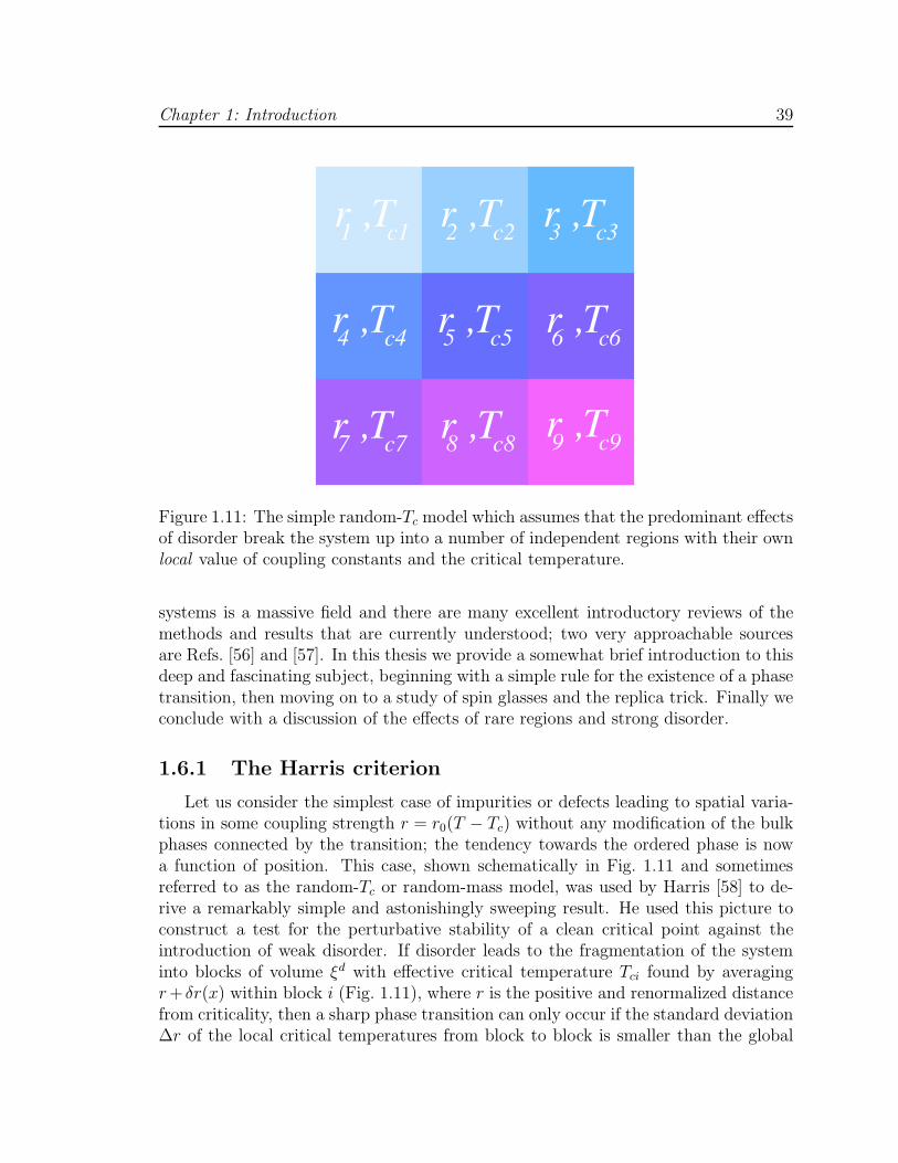
Chapter 1: Introduction 39
2 c2 r ,T3 c3
r ,T
r ,T
r ,T5 c5 r ,T6 c64 c4
7 c7 r ,T8 c8 r ,T9 c9
r ,T 1 c1 r ,T
Figure 1.11: The simple random-Tc model which assumes that the predominant effectsof disorder break the system up into a number of independent regions with their ownlocal value of coupling constants and the critical temperature.
systems is a massive field and there are many excellent introductory reviews of themethods and results that are currently understood; two very approachable sourcesare Refs. [56] and [57]. In this thesis we provide a somewhat brief introduction to thisdeep and fascinating subject, beginning with a simple rule for the existence of a phasetransition, then moving on to a study of spin glasses and the replica trick. Finally weconclude with a discussion of the effects of rare regions and strong disorder.
1.6.1 The Harris criterion
Let us consider the simplest case of impurities or defects leading to spatial varia-tions in some coupling strength r = r0(T − Tc) without any modification of the bulkphases connected by the transition; the tendency towards the ordered phase is nowa function of position. This case, shown schematically in Fig. 1.11 and sometimesreferred to as the random-Tc or random-mass model, was used by Harris [58] to de-rive a remarkably simple and astonishingly sweeping result. He used this picture toconstruct a test for the perturbative stability of a clean critical point against theintroduction of weak disorder. If disorder leads to the fragmentation of the systeminto blocks of volume ξd with effective critical temperature Tci found by averagingr + δr(x) within block i (Fig. 1.11), where r is the positive and renormalized distancefrom criticality, then a sharp phase transition can only occur if the standard deviation∆r of the local critical temperatures from block to block is smaller than the global

Chapter 1: Introduction 40
distance from the critical point r. For disorder with short range correlations (theblocks only interact at their boundaries) the central limit theory yields ∆r ∼ ξ−d/2
and assuming that ξ ∼ r−ν we have
∆r ∼ rdν/2. (1.86)
Thus for a transition to occur we must satisfy the Harris criterion: ∆r < r or
dν > 2. (1.87)
This criterion can be used to classify critical points based on the behavior of theaverage disorder strength as the length scale under consideration is increased.
(i) The Harris criterion dν > 2 is satisfied and the strength of disorder decreasesunder coarse graining with the system becoming asymptotically homogeneous atlong length scales. An example of this case, where all macroscopic variables areself-averaging is the three dimensional classical Heisenberg model with ν = 0.698[59].
(ii) Under renormalization, the relative disorder strength increases to some finitevalue and the system remains inhomogeneous. The critical point still exhibitsconventional scaling behavior but the critical exponents are modified such thattheir new values satisfy the Harris criterion. The width of the probability distri-bution for observables is no longer zero and they are consequently not self aver-aging. The three dimensional Ising model belongs to this case where ν = 0.627[60] in the clean system and shifts to ν = 0.684 [61] in the presence of disorder.
(iii) Finally, the relative magnitude of the randomness continues to increase with-out limit upon coarse graining with a fixed point characterized by an infinitedisorder strength. At this fixed point, the scaling is qualitatively modified tak-ing on a highly asymmetric exponential form and all probability distributionsbecome extremely broad, diverging with system size. Physical observables areno longer self-averaging but have averages dominated by rare events. Manifes-tations of such behavior occur in the McCoy-Wu model (Fig.1.12) [62, 63] andthe quantum random transverse field Ising model [64, 65].
Not surprisingly, most early work on disordered systems focused on cases (i) or (ii)where the average effects of disorder fluctuations on large length scales are small.Before returning to the very interesting case (iii), let us first briefly mention forcompleteness one of the most important weak disorder approaches which is suitableeven when the ordered phase is of a fundamentally different structure than its cleancounterpart.

Chapter 1: Introduction 41
1.6.2 Spin Glasses
A pedagogical review of classical disordered systems can be found in Refs. [66, 67],but it will be convenient to introduce some of their physical properties in terms ofa particular model consisting of Ising spins coupled randomly to all other spins; theSherrington-Kirkpatrick (SK) model [68]. It is described by the Hamiltonian
H = −1
2
∑
i,j
Jijσiσj (1.88)
where the exchange constants are randomly distributed according to
P (Jij) =1√
2πJ2exp
(J2
ij
2J2
)(1.89)
and it is the spread in the signs of the interaction parameters Jij that provides frustra-tion and can lead to glassy behavior. It is assumed that the variance of the couplingdistribution is not too large and such systems are referred to as “spin glasses”. Thepresence of disorder leads to an extraordinarily rough free energy landscape withmany nearly degenerate minima separated by large barriers, and one can imaginethree possible scenarios.
(i) The energy barriers separating the different minima are finite. The system canthus explore its phase space and will be paramagnetic (〈σi〉 = 0) although withpossibly slow dynamics.
(ii) A certain state could have a much lower free energy than all other states, andat low enough temperatures the system would freeze into this state. However,due to the presence of disorder, 〈σi〉 will still fluctuate from site-to-site and thetotal magnetization
m =1
N
∑
i
σi (1.90)
will be identically zero.
(iii) At low temperatures there exists a large number of states in which the systemcould be frozen into, separated by infinite energy barriers in the thermodynamiclimit.
Focusing on the third case, below some critical temperature, Tc, a phase transition ofergodicity breaking takes place and the energy landscape is divided into many valleysseparated by large (possibly infinite) energy barriers. At T = Tc − δT , each valleywill be characterized by a non-zero value of 〈σi〉(α) at each site where 〈· · · 〉(α) refers toa thermal average limited to valley α. In the presence of broken ergodicity, only such
Chapter 1: Introduction 42
restricted expectation values make sense and the order parameter which characterizesfreezing in each valley is
q =1
N
[∑
i
〈σi〉(α)
]2
(1.91)
where q is independent of the valley in the thermodynamic limit (N →∞) and goesto zero as T → Tc from below. The key point is that any further decrease in thetemperature leads to new ergodicity breaking phase transitions; each valley breaksinto smaller ones, separated by infinite energy barriers. This is a continuous processbelow Tc and within each infinite minimum, there may still be many finite valleys sothe spectrum of energy barriers goes smoothly to infinity. This hierarchical structureof minima is known as the ultrametricity of the spin glass state [69].
In Eq. (1.88), each spin can interact with every other spin and there is no conceptof space or a lattice; the SK model effectively lives in infinite dimensions. It is thismean field or maximally coupled behavior that allows for a solution and it can bestudied using a clever way of rewriting the partition function known as the replicatrick. For suitably weak disorder and at large length scales the free energy shouldbe a self-averaging quantity, and we are thus only interested in the logarithm of thepartition function averaged over disorder. We exploit a crafty way of writing thenatural logarithm,
lnZ = limn→0
Zn − 1
n(1.92)
and say that we have replicated the partition function n times, and Zn can nowbe straightforwardly averaged over the distribution of disorder, with translationalinvariance reappearing at the expense of generating additional interactions betweenreplicas. The replica method and replica field theory has formed the basis for a largeamount of the work done on random systems. Without serious consideration, it mightappear that the expectation values of physical observables should not depend on areplica index, this is known as the replica symmetric solution . However, this solutionoften leads to unphysical results (such as negative entropy) and we are ineluctablylead to consider more and more complicated methods of breaking replica symmetry.The physical origin of replica symmetry breaking may lay hidden in the limit n → 0required by Eq. (1.92) which does not necessarily commute with the thermodynamiclimit of infinite system size formally required for the existence of a phase transition.In addition, within replica field theory, many approaches are perturbative, and relyon the presence of only weak disorder. It is now becoming increasingly clear that foreven moderately strong randomness, an important role is played by rare but largedisorder fluctuations and the atypical spatial regions where they occur.

Chapter 1: Introduction 43
Figure 1.12: The McCoy-Wu model [62, 63] where each circle represents an Ising spinand although all horizontal bonds are equal, the vertical bonds are different in eachrow.
1.6.3 Rare region effects
The appearance of rare regions contributing to thermodynamic behavior was firstnoticed in the McCoy-Wu model [62, 63], a two dimensional Ising model with longrange disorder correlations in one dimension pictured schematically in Fig. 1.12. Thephysics can be more easily understood in a diluted classical Ising ferromagnet, asdepicted in Fig. 1.13. In the presence of dilution, the critical temperature Tc0 of theclean system, is reduced to Tc but in an infinitely large system there will always existarbitrarily large portions of the sample with volume VRR without any impurities (asseen in the highlighted portion of Fig. 1.13) with probability
P (VRR) ∼ e−pVRR (1.93)
where p is the impurity concentration. For all temperatures Tc < T < Tc0, these areaswill exhibit local magnetic order even though the bulk is paramagnetic. Griffithsshowed that these rare regions (RR) can lead to a singularity in the free energy, overan entire region of parameter space close to the transition now known as the Griffithsphase [70]. The type of singularity depends strongly on various details and in classicalsystems with short range disorder, the singularity is only essential leading to very weakthermodynamic Griffiths effects. Inside the Griffiths phase, the long time dynamics iscompletely dominated by rare regions leading to a spin-spin autocorrelation functionwhich decays as a power-law in time for the diluted ferromagnet considered here.
At a quantum phase transition, the rare regions become infinitely extended in theimaginary time direction (Fig. 1.14) precipitating even more sluggish fluctuations.The slow dynamics of rare regions can have a considerable effect, and in the presenceof completely static order, can even lead to the complete destruction of the phase

Chapter 1: Introduction 44
Figure 1.13: A diluted ferromagnet in the paramagnetic phase where the highlightedarea shows a region in the sample devoid of impurities which is strongly ordered andcan lead to a singularity in the free energy.
transition. The importance of RR physics in a given system depends on the relation-ship between the contribution of a single region to macroscopic observables and itssize. We can characterize this behavior by considering a single isolated rare regionwith linear size LRR that is locally in the ordered phase, that is, the local average barecoupling r defined along the lines of the random-mass model (Fig. 1.11) is negative.There are three distinct possibilities depending on the effective dimensionality, dRR
of the rare region, where dRR is the sum of both the temporal and spatial dimensionsof the droplet.
(i) If dRR < dLCD, where dLCD is the lower critical dimension, the rare regioncannot order independently of the rest of the system and its local couplingwill be renormalized to a positive value r > 0. The leading contributionsto all thermodynamic variables are controlled by at most a power of r whichcannot overcome the exponential scarcity of a RR. An example is found in anyclassical systems with point defects where dRR = 0; the rare regions are finitein dimension, and all their effects are subleading at the critical point.
(ii) If dRR = dLCD, the rare region cannot undergo a phase transition by itself,and although the renormalized coupling r is positive, it decreases exponentiallyquickly to zero with the volume of the region. The contribution to observables

Chapter 1: Introduction 45
Figure 1.14: The strongly ordered rare region from Fig. 1.13 extended a “length”Lτ = !β in imaginary time, Lτ →∞ at the quantum phase transition.
thus increases exponentially with size, exactly compensating for their exponen-tially suppressed probability in Eq. (1.93). The result is that the critical pointis dominated by rare regions, leading to exotic non-power law activated scaling.Examples include the McCoy-Wu model shown in Fig. 1.12 where the defectsare extended linear objects and dRR = 1, the lower critical dimension of the Isingmodel. The same is true for the quantum random transverse field Ising modelwhich has rare regions with spatial dimension zero, but temporal dimension oneat zero temperature.
(iii) If dRR > dLCD, the rare region can autonomously order, the renormalized cou-pling is negative and all dynamics freeze out as a static order parameter devel-ops. The global phase transition is destroyed by smearing due to different partsof the system ordering at different values of r. Classical three dimensional Isingmodels with planar defects exhibit such behavior as dRR = 2 and dLCD = 1[71, 72] as well as one dimensional quantum Ising models with suitably strongdamping [73, 74].
Very little analytical progress was made towards understanding the quantitativeeffects of rare regions until D.S. Fisher’s [64, 65] ingenious solution of the quantumrandom transverse field model using the strong disorder renormalization group pro-cedure of Ma, Dasgupta and Hu [75]. The details of his derivation are beyond thescope of this introductory chapter and are saved until Section 5.1.
We have argued that disorder can have profound implications for critical phenom-

Chapter 1: Introduction 46
ena ranging from small quantitative changes arbitrarily close to criticality, all theway to causing exotic non-power law activated dynamic scaling or the complete de-struction of the phase transition. This section has attempted to provide an overviewof this phenomenology with special focus on the effects of rare regions characterizedby the relationship between their size and the lower critical dimension. The connec-tion will be revisited in Chapter 5 when we find compelling evidence for an infiniterandomness fixed point and activated scaling at the superconductor-metal quantumphase transition.
1.7 Organization
This rest of this thesis is composed of four chapters providing details on methodsand results and a final concluding chapter.
We begin by introducing a particular continuum quantum field theory for thesuperconductor-metal quantum phase transition in nanowires in terms of a Cooperpair order parameter and discuss a number of its general properties through a scalinganalysis. The relationship between its coupling constants and microscopic quantitiesis discussed with specific details provided on their values in the clean and dirty limit.In the approximation where the number of components of the order parameter islarge, we perform a detailed study of the electrical and thermal transport propertiesof ultra-narrow wires throughout the phase diagram. We next discuss a systematicexpansion that can be performed for a finite number of order parameter componentsand find fluctuation corrections to various results near criticality. Finally we introducequenched disorder into our theory and find evidence for infinite randomness andactivated scaling. We conclude with some general observations on the diverse types ofphysics on display at the superconductor-metal transition and discuss some promisingavenues for future research.

Chapter 2
Dissipative Theory of theSuperconductor-Metal Transition
This chapter will focus on a possible model for the quantum phase transitionbetween a superconductor and a metal (a SMT). The physical system of interest,as studied in numerous recent experiments [35, 45, 38, 76, 77, 44, 78, 39, 37] andintroduced in Chapter 1, is a quasi-one dimensional nanowire, of length L with alarge number of transverse conduction channels, N⊥. This guarantees that surfaceeffects will not be particularly destructive, and that the electronic localization lengthξloc, given by ξloc = N⊥3 is much larger than the mean free path 3.
From the Cooper instability in BCS theory we know that the existence of a non-trivial quantum critical point in a metal implies a finite electron interaction strength.Naively the existence of interactions would seem to preclude the possibility of anyquantum phase transition between a superconductor and a metal because the orderedphase will exist at all strictly non-zero temperatures for arbitrarily weak paring (seeEq. (1.21)). Moreover, if the temperature is driven to zero in a pure BCS supercon-ductor pair fluctuations will be completely eliminated [79]. The solution arrives inthe form of pair-breaking interactions, or any perturbation that is odd under timereversal, which act differently on the spin and momentum reversed constituents ofa Cooper pair. The presence of these interactions effectively cuts of the logarithmicsingularity in the pair susceptibility and sets a critical value for the strength of thepair potential before superconductivity can develop. Therefore, our proposed SMTmust live in the pair-breaking universality class.
As discussed in the introduction, the mean-field theory for the SMT goes back tothe early work [41] of Abrikosov and Gor’kov (AG). In one of the preliminary discus-sions of a quantum phase transition, they showed that a large enough concentrationof magnetic impurities could induce a SMT at T = 0. It has since been shown thatsuch a theory applies in a large variety of situations with pair-breaking perturba-tions: anisotropic superconductors with non-magnetic impurities [80, 81, 82], lower-dimensional superconductors with magnetic fields oriented in a direction parallel to
47

Chapter 2: Dissipative Theory of the Superconductor-Metal Transition 48
the Cooper pair motion [83, 84], and s-wave superconductors with inhomogeneity inthe strength of the attractive BCS interaction [43]. Indeed, it is expected that pair-breaking is present in any experimentally realizable SMT at T = 0. In the nanowireexperiments, explicit evidence for pair-breaking magnetic moments on the wire sur-face was presented recently by Rogachev et al. [37] and in Section 1.4.2 we describedan avenue by which they could lead to the destruction of superconductivity as theradius of the wire is reduced.
Fluctuations about the AG theory have been considered [85, 86, 87, 83, 84] in themetallic state, and lead to the well-known Aslamazov-Larkin (AL), Maki-Thompson(MT) and Density of States (DoS) corrections to the conductivity. The form of thesecorrections is usually introduced in terms of the structure of their diagrammaticrepresentation within the finite temperature disordered electron perturbation theorybut they all have the same physical origin: in the presence of strong pair-breaking,the normal metal still experiences pairing fluctuations near the Fermi surface as aresult of its proximity to the superconducting state. Specifically, the AL effect comesfrom the direct charge transfer from fluctuating Cooper pairs, the MT correctionresults from coherent Andreev scattering off the fluctuating pairs and the Densityof States (DoS) correction is due to the reduction of the normal electron densityof states near the Fermi surface accounting for the paired electrons [88]. At theSMT, field-theoretic analyses [89, 90] show that the AG theory, along with the AL,MT and DoS corrections, is inadequate in spatial dimension d ≤ 2, and additionalrepulsive self-interactions among Cooper pairs have to be included. Here, d definesthe dimensionality of the Cooper pair motion. The confining dimension, or radiusof the wire, R, is larger than the inverse Fermi wavevector, but smaller than thesuperconducting coherence length or Cooper pair size, ξ. This is the exact conditiondiscussed in the introduction for the quasi-one dimensional limit. While the Cooperpairs are effectively one dimensional, any unpaired electrons have a three dimensionalFermi surface and thus strictly 1d Luttinger liquid physics do not apply.
In the remaining chapters of this thesis, we will examine the d = 1 SMT forboth a clean and disordered wire in great detail. We will find that the transition isdescribed by a strongly-coupled field theory of bosonic Cooper pairs, overdamped bytheir coupling to the fermionic quasiparticles (normal electrons).
As our goal is to understand the aforementioned experiments on ultra-thin metallicwires and we are interested in the fluctuation corrections to the thermal and electri-cal conductivity across the SMT as well as the nature of the crossovers from thisuniversal quantum critical physics to previously studied regimes at low T about thesuperconducting and metallic phases. To frame the discussion in the duration of thischapter, the full crossover phase diagram is summarized in Fig. 2.1. The importantfeatures of the global pair-breaking phase diagram are as follows. On the metallic sideof the transition, there is a crossover to a low T regime described by the theory [83] ofAL+MT+DoS corrections in d = 1 (dashed line in Fig. 2.1). On the superconductingside, there is a regime of intermediate temperatures where the classical phase slip

Chapter 2: Dissipative Theory of the Superconductor-Metal Transition 49
FSC
LAMH
α
T
Mαc
QC
Figure 2.1: Crossover phase diagram of the superconductor-metal transition in aquasi-one dimensional superconductor. The metal (M) is described by the pertur-bative theory of Ref. [83]. The quantum critical (QC) region is described by oureffective theory Sα for temperatures above Tdis where the effects of disorder may beneglected. The Mooij-Schon mode is present everywhere, but couples strongly tosuperconducting fluctuations only in the fluctuating superconductor (FSC) regime,where it is described by Eq. (2.31); note that Sα does not apply here. The dashedlines are crossover boundaries which occur at T ∼ |α− αc| (from Eq. (2.11)) and theintermediate LAMH region should be described by the theory of thermally activatedphase slips discussed in Chapter 1 with the possible modifications of Chapter 3.
theory of Langer, Ambegaokar, McCumber, and Halperin (LAMH) applies [19, 20],and eventually another crossover at still lower temperatures to a phase fluctuatingregime whose description requires a non-linear σ-model of fermion pair fluctuationscoupled to the superconducting order [91]. Intermediate between these regimes is thequantum criticality we describe here, in which phase and amplitude fluctuations mustbe treated on equal footing.
In the rest of this chapter, we present details of the dissipative theory which willbe used as the starting point for all computations in this thesis. After a brief scalinganalysis, the role of particle-hole symmetry and the Mooij-Schon [92] mode is dis-cussed, as well as the relationship between the model parameters and the microscopicBCS theory. Finally, the effects of the Cooper pair self-interactions on universalitythroughout the quantum critical regime and the role of disorder are highlighted.

Chapter 2: Dissipative Theory of the Superconductor-Metal Transition 50
2.1 Dissipative model
The approach to the SMT taken here is akin to previously studied theories [93,94, 95] of disordered superconducting films with unconventional pairing symmetry.Such films are assumed to be composed of a network of small Josephson coupled su-perconducting islands. The transition between the normal and superconducting statecan be tuned by altering the distance between the grains; if the separation becomeslarge enough, quantum fluctuations can destroy superconducting order even at zerotemperature. Physically, the transition occurs when the Josephson coupling becomesless than the Coulomb energy due to the transfer of a single Cooper pair betweenislands. These arguments can be made more rigorous by starting from microscopicBCS theory and deriving an effective model for the fluctuations of the Cooper pairorder parameter. The order parameter is strongly overdamped by decay into quasi-particle excitations manifest as an interaction that is long range in imaginary time[80, 79, 83, 84, 43].
These ideas can be directly applied to the d = 1 quantum superconductor-metaltransition in the pair-breaking universality class which is relevant for ultra-narrowquasi one-dimensional metallic wires. The physical ingredients include repulsivepaired states and a lack of charge conservation of the condensate requiring the ex-istence of a semi-infinite bath (the large number of transverse conduction channels)into which the former member electrons of a disassociated Cooper pair can flow intoupon breaking. The final description will be in terms of a strongly-coupled field the-ory of bosonic Cooper pairs, overdamped by their coupling to the normal unpairedfermionic states of the metal.
It turns out that the fluctuation corrections to transport associated with the ALcorrection discussed above are naturally captured in this picture. These have [83,84] a Cooper pair propagator (Dk2 + |ωn| + α)−1 at wavevector k and imaginarybosonic Matsubara frequency iωn in the metal in both the clean and dirty limits.Here, the “mass” or pair-breaking frequency α measures the strength of the pair-breaking interaction which could come from a variety of sources as mentioned in theintroduction. D is equal to the usual diffusion constant D = D = vF3/3 (vF is theFermi velocity) in the dirty limit where the mean free path is much smaller than thesuperconducting coherence length (3* ξ0). In the clean limit, where 3. ξ0, D willbe in general some non-universal number that depends on the specific microscopicdetails (such as the lattice constant) of the system in question. This motivates thequantum critical theory of Ref. [89, 96] for a field Ψ(x, τ) which represents the local

Chapter 2: Dissipative Theory of the Superconductor-Metal Transition 51
Cooper pair operator
Sα =
L∫
0
dx
1/T∫
0
dτ[D|∂xΨ(x, τ)|2 + α|Ψ(x, τ)|2 +
u
2|Ψ(x, τ)|4
]
+ T∑
ωn
L∫
0
dx γ|ωn||Ψ(x,ωn)|2,
(2.1)
where we have used the temporal Fourier transform of Ψ(x, τ)
Ψ(x,ωn) =
1/T∫
0
dtΨ(x, τ)eiωnτ . (2.2)
with ωn = 2πnT to more compactly express the non-locality of the dissipative termin imaginary time and we will work in units where ! = kB = 1 for convenience.From this point forward, we will suppress the limits of integration for the sake ofcompactness unless their inclusion is required for clarity. The quartic coupling u mustbe positive to ensure stability, and describes the repulsion between Cooper pairs. Thepairs are strongly overdamped, and the rate of their decay into the metallic bath ischaracterized by the coupling constant multiplying the |ωn| term, γ, which is requiredto be positive by causality. It will be convenient to rescale the field Ψ such that thecoefficient of the Landau damping term is equal to unity. In addition, we rescale allcouplings according to
Ψ→Ψ√γ
; D → γD; α→ γα; u→ γ2u. (2.3)
This theory describes the vicinity of a superconductor-metal quantum critical point,corresponding to the (bare) value z = 2 for the dynamic critical exponent. A differentdescription (z 3= 2) cannot be completely ruled out, but it would most likely requireadditional tuning parameters as well as the inclusion of unusual pairing phenomenalike gapless superconductivity [79].
The transition is driven by altering the strength of the pair-breaking frequencyα as was shown schematically in Fig. 2.1. As α is reduced, the quantum criticalpoint, αc is defined as the special value where the Cooper pair operator first acquiresa non-zero expectation value, 〈Ψ(x, τ)〉Sα 3= 0. For α > αc there is normal metallicconduction, while for α < αc both thermal and quantum phase slips, included underthe guise of amplitude fluctuations of Ψ destroy the superflow.
The field theory in Eq. (2.1) is identical in form to the Hertz-Millis-Moriya theory[47, 97, 98] describing the Fermi liquid to spin-density wave (SDW) transition, withthe Cooper pair operator Ψ replaced by an O(3) order parameter representing diffusive

Chapter 2: Dissipative Theory of the Superconductor-Metal Transition 52
paramagnons. In the neighborhood of this transition, k measures the magnitude ofthe deviation from the SDW ordering wave vector K and the dissipative |ωn| termarises from the damping of order parameter fluctuations resulting from coupling togapless fermionic excitations of the metal near points on the Fermi surface connectedby K. A more careful analysis leads to the realization that at T = 0 on the ordered(SDW) side of the transition, a gap appears in the fermion spectrum for small k. Thus,this description is only fully accurate at T = 0 on the disordered (metallic) side ofthe transition or at finite temperature in the quantum critical regime above the SDWstate. The same logic applies to the role of phase fluctuations at low temperaturesin the superconducting phase near the SMT. We will return to this point later witha thorough discussion of the Mooij-Schon normal mode, but for now we begin with adetailed scaling analysis of Sα.
2.2 Scaling analysis
Let us rewrite the rescaled version of Eq. (2.1) via Eq. (2.3) in d dimensions
Sα =
∫ddx
∫dτ[D|∂xΨ(x, τ)|2 + α|Ψ(x, τ)|2 +
u
2|Ψ(x, τ)|4
]
+ T∑
ωn
∫ddx |ωn||Ψ(x,ωn)|2.
(2.4)
The anisotropic relationship between space and time allows us to identify the dynam-ical critical exponent z = 2 implying that dim[ωn] = dim[T ] = z so simple powercounting leads to
dim[Ψ] =d
2(2.5a)
dim[α] = 2 (2.5b)
dim[u] = 2− d (2.5c)
where dim[· · · ] is the scaling dimension introduced in Section 1.5.4. From the scalingdimension for u we can immediately identify the lower critical dimension of the SMTas d = 2. By definition, for d > 2 the quartic coupling is irrelevant, and all physicalproperties could be computed perturbatively in the (small) value of u, resulting inu-dependent non-universal results. d = 2 is marginal, and for the case consideredhere, d = 1, u is a relevant perturbation, and we will need to employ alternatemethods. However, in the strong coupling regime (u →∞) we can expect results tobe universal.
Pankov et al. [99] studied a theory similar to Sα with Ψ replaced by an O(N)field φa via the renormalization group (RG) in an ε = 2 − d expansion in one andtwo dimensions at zero temperature. The most important result obtained from their

Chapter 2: Dissipative Theory of the Superconductor-Metal Transition 53
RG analysis is that the damping term, |ωn|, generated from the long-range 1/τ 2
interaction between order parameter fluctuations does not require an independentrenormalization, and thus the frequency dependence of the propagator only involveswavefunction renormalization. At T = 0 and α = αc in one dimension, they find anon-trivial fixed point and an analysis of the RG equations leads to an expression forthe dynamical susceptibility at small frequencies and momenta
χ(k,ω) =
∫dτ
∫dx〈φa(x, τ)φa(0, 0)〉e−i(kx−ωτ)
= k−2+ηΦχ
( ω
ck2−η
)(2.6)
where Φχ is a universal scaling function. This is simply Eq. (1.83) with the scalingdimension of the susceptibility dim[χ] = 2 − η. The constant c turns out to beuniversal
c =(N + 2)[6π2 ln 2− 11ζ(3)]
1728(2.7)
with ζ(x) the Riemann zeta function and N the number of real order parametercomponents.
These results carry through to the study of our effective action, Eq. (2.4) with theonly modification being that c changes to a non-universal number due to the presenceof D. From Eq. (2.6) and Eq. (1.83), the modified dynamical critical exponent canbe read off as
z = 2− η (2.8)
where η is the anomalous dimension; a result which holds to all orders due to theexistence of only wavefunction renormalization [99, 100]. This scaling form can begeneralized to finite temperatures (see Eq. (1.85) with r = rc and ! = kB = 1) wherewe expect
χ(k,ωn, T ) =1
TΦχ
(ωn
T,
c1k
T 1/z
), (2.9)
with Φχ another universal scaling function and c1 a non-universal constant. Mostinterestingly, at k = 0 and ω = 0 the value of the inverse susceptibility in thequantum critical region will be fixed by temperature alone,
χ−1(0, 0) = C1T (2.10)
and the highly non-trivial universal constant C1 will be computed in a 1/N expansionin chapter 4.
Scaling functions for the most singular parts of the dc electrical σ and thermal κconductivities can also be derived with a knowledge of their scaling dimensions alone.We know that in one dimension, the conductivity is equal to e2/h times a length,and for k = ωn = 0 but finite temperature we have only one length scale available to

Chapter 2: Dissipative Theory of the Superconductor-Metal Transition 54
us, the thermal length, L1/zτ . Similar considerations for the thermal conductivity in
conjunction with Eq. (1.85) allow us to write
σ =e2
!
(kBT
!D
)−1/z
Φσ
([!(α− αc)]ν
(kBT )1/z
)(2.11)
and
κ =k2
BT
!
(kBT
!D
)−1/z
Φκ
([!(α− αc)]ν
(kBT )1/z
)(2.12)
where z = 2 and ν = 1/2 in the Gaussian limit and we have returned to real physicalengineering units. If we include interactions but perform calculations in the large-Nlimit, z is unchanged, but ν = 1 and one would need to replace
[!(α− αc)]ν
(kBT )1/z→
!(α− αc)
(kBT )2/zν(2.13)
in the scaling functions. Upon comparing Eq. (2.11) with the microscopic resultfor the conductivity calculated within perturbation theory [83, 84] and reproduced inEq. (3.4) we see that the the most divergent contribution at T > 0 but for |α−αc|* 1,corresponding to the AL correction of the direct contribution of Cooper pairs to themetallic conductivity is included in our critical theory.
This section has unequivocally demonstrated the power and utility of scaling anduniversality, allowing us to derive scaling forms for the finite temperature dynamicorder parameter susceptibility as well as the electrical and thermal conductivity withalmost no effort in terms of the critical exponents ν, η and z. We now provide somepreviously determined analytical and numerical results for their values.
The anomalous dimension η and correlation exponent ν defined by ξ ∼ |α−αc|−ν ,can be computed in the ε = 2− d expansion [99, 89] and are found to be
η =(N + 2)(12− π2)
4(N + 8)2ε2 + O(ε3) (2.14)
ν =1
2+
(N + 2)
4(N + 8)ε
+(N + 2)[6N2 + (228− 7π2)N + 792− 38π2]
48(N + 8)3ε2 + O(ε3). (2.15)
These results are in agreement with Monte Carlo simulations [101] which found z =1.97(3), z + η = 1.985(20) and ν = 0.689(6). The exponents ν and η can also becomputed in the 1/N expansion and the results are detailed in chapter 4.
The main results of this section, and the analysis of Ref. [99] is that Sα satisfiesconventional hyperscaling relations at the T = 0 SMT in the absence of disorder.This implies that we can neglect any irrelevant operators, and transport should be

Chapter 2: Dissipative Theory of the Superconductor-Metal Transition 55
fully described by Eq. (2.4). Moreover, the most singular part of the dc conductivityof a given wire will be described by Eq. (2.11) which is independent of its length L.The is a consequence of the dominant physics in the quantum critical regime beingcontrolled by low energy superconducting fluctuations with a characteristic lengthscale equal to the extent of the wire [89] itself.
2.3 Particle-hole asymmetry
In the scaling analysis of the previous section, we neglected an important detail;for z = 2, when the energy dependence of the electronic density of states near theFermi level is included, a propagating term in the action can arise from the weakparticle-hole asymmetry of the electronic spectrum
Sη =
∫dx
∫dτηΨ∗(x, τ)
∂
∂τΨ(x, τ). (2.16)
The magnitude of particle-hole symmetry breaking, η is proportional to the energyderivative of the density of states at the Fermi energy, and we therefore expect itsbare value to be small. This is supported by the fact that our quasi-one dimensionaltreatment of Cooper pairs coupled to a bath composed of three dimensional electrons,required the ratio of the pairing to Fermi energy to be small. In fact, a microscopicweak coupling derivation of Eq.(2.4) for a dirty two dimensional superconductor withd-Wave pairing symmetry [80] finds that the ratio of the dissipative to propagativeterms is proportional to the dimensionless conductivity of the normal phase, η ∝1/εFτ where τ is the scattering time in the self-consistent Born approximation. Fora good metal, the product of the scattering time and Fermi energy is large, and thusη * 1. This is consistent with results at finite temperature for a weak-coupling shortcoherence length superconductor [102].
At tree level, η is marginal, and as just argued, we expect its bare value to besmall. However, we can examine the renormalization group fate of Sη near the fixedpoint of Sα. The scaling dimension of η can be computed in a d = 2 − ε expansionfor a massless (α = 0) quantum critical theory through the conventional methodof isolating any logarithmic singularities (or 1/ε poles) in the Feynman diagramscorresponding to all possible insertions of the perturbing term, iηω. For the caseconsidered here, there are two unique graphs
2
iω1
+iω1
(2.17)

Chapter 2: Dissipative Theory of the Superconductor-Metal Transition 56
where a solid line is equal to the bare propagator (k2 + |ω|)−1, a dot represents thequartic interaction u and a cross is an insertion coming from Eq. (2.16).
If the external lines have frequency Ω and zero momentum, then the combinationof these graphs leads to the integral
I(Ω) = −i2ηu2
∫dω1
2π
∫dω2
2π
∫ddk
(2π)d
∫ddq
(2π)d
×ω1
(k2 + |ω1|)2(q2 + |ω2|)[(k + q)2 + |ω1 + ω2 + Ω|].
(2.18)
A simple power counting analysis of the integrand in d = 2 − ε dimensions leads tothe appearance of the predicted pole
I(Ω) = iΩηA
2ε, (2.19)
where as usual, the flow equation for η is related to the residue A via
dη
d3= Aη. (2.20)
Doing the two momentum integrals by employing Feynman parameters we find
I(Ω) = −i2ηu2Γ(4− d)
(4π)d
1∫
0
dx
1∫
0
dy
∫dω1
2π
∫dω2
2π
(1− y)y1−d/2
[1− y(x2 − x + 1)]d/2
×ω1
[(1− y)|ω1| + y(1− x)|ω2| + xy|ω1 + ω2 + Ω|]4−d.
(2.21)
where Γ(x) is the gamma function. The double frequency integral, can be done bydetermining the sign of the various absolute values in the relevant seven regions ofthe ω1 − ω2 plane, leading to the following useful but complicated looking result
Iω(A, B, C, σ) =
∫dω1
2π
∫dω2
2π
ω1
(A|ω1| + B|ω2| + C|ω1 + ω2 + Ω|)σ
= −ABCΓ(σ − 3)Ω3−σ
π2Γ(σ)
A3−σ
[2(2A2 −B2 − C2)
(A2 − B2)2(A2 − C2)2
−3− σ
A2(A2 − C2)(A2 − B2)
]− B3−σ
[2
(B2 − C2)(A2 − B2)2
]
+ C3−σ
[2
(B2 − C2)(A2 − C2)2
]. (2.22)
In d = 2− ε and σ = 2 + ε, Iω has a pole at ε = 0 with a residue that can be read offfrom
Iω(A, B, C, 2 + ε) = −Ω
π2
[BC(2A + B + C)
(A + B)2(A + C)2(B + C)
]1
ε+ O(1). (2.23)

Chapter 2: Dissipative Theory of the Superconductor-Metal Transition 57
Using Eq. (2.23) in Eq. (2.21) we find
I(Ω) =iΩu2
8π4ε
1∫
0
dx
1∫
0
dyxy(1− x)(1− y)(2− y)
[1− y(x2 − x + 1)][1− y + xy2(1− x)]2
=iΩu2η
8π4ε
(π2
4− 2
)(2.24)
and comparing with Eq. (2.20) we can read off the flow equation
dη
d3=
u2
16π2
(1−
8
π2
)η. (2.25)
The fixed point value of u is given in Ref. [99] for the equivalent z = 2 O(N)model with the change of notation u0 = 3u. Equivalently it can be easily computedto one loop order as
u∗ =2π2
5ε (2.26)
leading todη
d3=ε2
100(π2 − 8)η (2.27)
or η(3) ∼ e0.02ε2/ at RG scale 3. Thus we conclude that although η is relevant, itsscaling dimension is extremely small. In conjunction with a bare value that we haveargued should be small, we will neglect Sη in future calculations.
There is still one piece missing in our analysis of Sα as alluded to in the previoussection; the role of charge conservation (which Sα breaks) and the associated normalmodes.
2.4 Phase fluctuations
Models similar to Eq. (2.1), but lacking amplitude fluctuations (so called phase-only theories) have been previously applied to the physical situation considered here[32, 103, 104, 105, 106]. In these continuum theories, the destruction of supercon-ductivity is due to the proliferation of quantum phase slips resulting in a normalphase which we maintain is insulating and not metallic at T = 0. Such theories maydescribe a quantum superconductor-insulator transition (SIT) which could be appro-priate in short inhomogeneous wires. The superfluid’s conductivity will be controlledby irrelevant phase-slip operators since the resulting d = 1 SIT in this descriptionlives in the Kosterlitz-Thouless universality class [107].
From hydrodynamic arguments, we know that a one-dimensional metal or super-conductor should support a gapless plasmon, or a Mooij-Schon normal mode [92],which disperses as ω ∼ k ln1/2(1/(kR)). Our discussion of this issue parallels that in

Chapter 2: Dissipative Theory of the Superconductor-Metal Transition 58
Refs. [108, 109] on the role of conservation laws in the critical fluctuations of quantumtransitions in metallic systems for which the order parameter is overdamped (as isthe case here). We couple Ψ to a fluctuating scalar potential Aτ with bare action
SA =
∫dk
2π
∫dω
2π
|Aτ (k,ω)|2
4 ln(1/(kR)). (2.28)
However, the nature of the Aτ -Ψ coupling differs between the “quantum critical”and “fluctuating superconductor” regimes of Fig. 2.1. For the main results of thisstudy, we need only the coupling in the quantum critical region, where the physics ofthe plasmon mode is unchanged from that in the “Metal” region of Fig. 2.1. Afterintegrating out the fermions, we obtain the Aτ action
SΠ =
∫dk
2π
∫dω
2π
1
2Π(k,ω)|Aτ(k,ω)|2, (2.29)
where Π is the irreducible density correlation function (the “polarizability”) of themetal. For ω . k, we have Π(k,ω) ∼ k2/ω2, and then SA + SΠ has a pole at theplasmon frequency noted above. We also observe that the coupling between these Aτ
fluctuations and Ψ is negligible: a slowly varying Aτ is a shift in the local chemicalpotential, and to the extent we can ignore the variation in the electronic density ofstates at these energy scales, the effective couplings in Sα do not change with Aτ ,and there is no Aτ − Ψ coupling. The existence of an Aτ − Ψ coupling non-analyticin frequency has been discussed by Ioffe and Millis [108]. However, they show byWard identities, which also apply here, that these couplings do not contribute to thephysical charge correlations. So, in the quantum critical region, Sα and SA + SΠ areindependent theories describing the pairing and charge fluctuations respectively.
As described in the previous section, the coupling constant which measures particle-hole asymmetry is formally, albeit weakly relevant (see Eq. (2.27)) and thus a smallAτ −Ψ coupling appears by making the τ -derivative in Eq. (2.16) Gauge covariant
Sη =
∫dxdτ
[ηΨ∗
(∂
∂τ− 2eiAτ
)Ψ
]. (2.30)
However, the combination of the small scaling dimension and the small bare valueof η implies that such particle-hole asymmetric effects, and the consequent couplingbetween pairing and charge fluctuations, can justifiably be ignored in theories hopingto describe realistic experiments.
We conclude by addressing the physics in the “Fluctuating superconductor” regimeof Fig. 2.1 for α < αc. Now coupling between the pairing and charge fluctuations ismuch stronger. When T < (αc − α) the action Sα does not apply for the smallestfrequencies. The reasons for this are again analogous to arguments made for the spin-density-wave ordering transition in metals, as discussed in Section 2.1 and Ref. [48].

Chapter 2: Dissipative Theory of the Superconductor-Metal Transition 59
For the latter case, it was argued that with the emergence of long-range spin den-sity wave order, the low energy fermionic particle-hole excitations at the orderingwavevector were gapped out, and so the diffusive paramagnon action applied onlyfor energies larger than this gap. At energies smaller than the gap, spin-waves withdispersion ω ∼ k emerge. In the superconducting case, there is no true long-rangeorder at any T > 0, but the order is disrupted primarily by ‘renormalized classical’thermal fluctuations of the phase, φ of the complex Ψ field. We assume that there is alocal pairing amplitude in the fermion spectrum, analogous to the spin-density waveorder. The low energy effective action for φ obtained by integrating the fermions inthe presence of a local pairing, is
Sφ =
∫dxdτ
[K1(∂τφ− 2eAτ )
2 + K2(∂xφ)2]
(2.31)
where K1,2 vanish as power of (αc−α) [109]. The strongly coupled pairing and chargefluctuations in the “Fluctuating superconductor” regime of Fig. 2.1 are described bySA + Sφ, and this theory contains the Mooij-Schon mode, which is the analog ofthe ‘spin-wave’ mode. We do not claim that SA + Sφ can extended across quantumcriticality into the normal phase, in contrast to other works [32] which consider vortexunbinding in such a theory.
The arguments presented in this section strive to justify the use of Sα throughoutthe quantum critical regime, and we now make a slight aside to discuss the relationshipbetween the parameters of the theory, α, γ, u and D to those of the microscopic BCStheory.
2.5 Connection to microscopic BCS theory
In order to motivate the experimental relevance of the effective action Sα, wewould like to determine the microscopic values of the pair-breaking frequency α, thebare diffusion constant D, dissipation strength γ and quartic coupling u in both theclean and dirty limits. We begin with the connection of the pair-breaking frequency tovarious experimentally relevant geometries, then move on to the relationship betweenour theory and a time dependent Ginzburg-Landau (TDGL) theory for a conventionalsuperconductor.
2.5.1 Pair-breaking in quasi-one dimensional wires
As mentioned in the Section 1.4, one can consider pair-breaking perturbationscoming from a variety of sources. The most theoretically appealing consists of mag-netic impurities localized on the surface of a metallic wire leading to an inhomoge-neous BCS coupling (Fig. 1.7). In this case, the microscopic value of α is not knownexactly, but it can be related to the inverse of the spin-flip scatting time. However,

Chapter 2: Dissipative Theory of the Superconductor-Metal Transition 60
H
Figure 2.2: Two possible geometries discussed in the introduction, consisting of ametallic nanowire or a cylinder (formed by coating an insulating core) with a diameteron the order of the zero temperature BCS coherence length in a longitudinal magneticfield.
there are a number of well-defined experimental geometries where one can computethe actual value of α in terms of the physical properties of the system. Two such caseswhich are of interest here were previously introduced, along with some experimentalmanifestations. These include a narrow metallic wire or multiply connected metalliccylinder in a parallel magnetic field, schematically shown in Fig. 2.2.
In the dirty limit, Shah and Lopatin [84] have computed the precise form of αthrough the use of the Usadel equation formalism. They find that for a narrowdiffusive wire with radius R smaller than both the superconducting coherence lengthand the magnetic penetration depth placed in a parallel magnetic field H ,
αwire =D
2
(eHR
c
)2
(2.32)
where D is the diffusion constant and c the speed of light. Alternatively, for a multiplyconnected cylinder of inner radius R1 and outer radius R2 in a parallel magnetic fieldthey find
αcyl = D
eH
4c
[eH
c(R2
1 + R22)− 4n
]+ n2 ln(R2/R1)
R22 −R2
1
, (2.33)
where n is the integer that minimizes the superfluid velocity for a given value thetrapped flux. As mentioned in Chapter 1, the former geometry is relevant to themeasurements of Rogachev et al on Tc suppression in MoGe nanowires [44] in aparallel magnetic field (Fig. 1.8), while the in-field phase diagram of ultra-thin Aland Au0.7In0.3 cylinders has been measured in Ref. [45] (Fig. 1.9).
2.5.2 Microscopic parameters in the clean and dirty limits
The microscopic values of D ,γ and u can be found through an analysis of the timedependent Ginzburg-Landau theory studied by Tucker and Halperin [110]. There, the
Chapter 2: Dissipative Theory of the Superconductor-Metal Transition 61
three dimensional equation of motion for the Cooper pair operator Ψ(x, t) in real timeis given by
!γ∂
∂tΨ(x, t) = −
[a + b|Ψ(x, t)|2 + δ(−i∇)2
]Ψ(x, t). (2.34)
Rescaling, to ensure that the coefficient of the time derivative term is unity (as wehave done in Eq. (2.4), and performing an integral over the cross-sectional area of thewire to move to the quasi-one dimensional case of interest (Ψ(x, y, z, t) ∼ Ψ(x, t)), weread off the value of the coupling constants to be
D =δ
!γ(2.35a)
u =b
A!2γ2(2.35b)
where A is the cross-sectional area of the wire. Appendix A of Ref. [110] gives themicroscopic values of δ, b and γ as
δ =!2
2m, (2.36a)
b =!2
2mξ2(0)
2
Nχ(0.882ξ0/l), (2.36b)
γ =π!2
16mξ2(0)kBTc0. (2.36c)
where ξ(T ) is the Ginzburg-Landau coherence length, ξ0 the BCS coherence length,3 the mean free path and χ(ρ) the Gor’kov function defined by
χ(ρ) =∞∑
n=0
1
(2n + 1)2(2n + 1 + ρ)
[∞∑
n=0
1
(2n + 1)3
]−1
. (2.37)
The critical temperature and density of conduction electrons in the normal state areknown to be
1
kBTc0=
ξ00.18!vF
; (2.38a)
N =k3
F
3π2(2.38b)
respectively, while, the zero temperature coherence length and relevant Gor’kov func-tion depend on whether we are in the clean or dirty limit
ξ(0) =
0.74ξ0 ; ξ0 * 3
0.85√ξ03 ; ξ0 . 3
, (2.39a)
χ(0.882ξ0/l) =
1 ; ξ0 * 3
1.333/ξ0 ; ξ0 . 3. (2.39b)

Chapter 2: Dissipative Theory of the Superconductor-Metal Transition 62
We have now gathered all the required information to compute the actual microscopicvalues of our model parameters in the dirty (ξ0 . 3) and clean (ξ0 * 3) limitsdifferentiated by the subscripts d for dirty and c for clean.
Dirty limit (ξ0 . 3)
Using the above relations, we find that for the dirty limit
Dd = D =1
3vF3 (2.40a)
γd +1.5
kF3(2.40b)
ud + 2.9vF
!N⊥(2.40c)
where the number of transverse conduction channels is assumed to be large, and isgiven by
N⊥ =2k2
FA
3π. (2.41)
Clean limit (ξ0 * 3)
Similarly, in the clean limit
Dc =1
4vF ξ0 (2.42a)
γc +2.0
kFξ0(2.42b)
uc = ud + 2.9vF
!N⊥(2.42c)
where we note that the bare value of the quartic coupling is identical in both limits.The value of these parameters clearly depends on the particular normalization schemechosen for the order parameter, but the final results for all physically measurablequantities, such as the conductivity, will obviously be normalization independent.
With these values computed, we may now discuss the role of Hartree corrections toour theory, that is, the temperature range where the quartic interaction u is stronglyrelevant and universal results may be expected.
2.6 Universality in the quantum critical regime
The microscopic theory of the superconductor-metal transition was consideredin great detail by Shah and Lopatin [84] in a Gaussian theory of superconductingfluctuations that corresponds to the effective field theory presented here with u set

Chapter 2: Dissipative Theory of the Superconductor-Metal Transition 63
to zero. In Chapter 3 we will compare the transport properties computed from theeffective action Sα with Shah’s results in the metallic regime where α . αc butarmed with the microscopic values of our model parameters we can make a numberof observations regarding the validity of the non-interacting theory in the stronglyfluctuating quantum critical regime (which they refer to as the classical regime). Thekey point is their use of the mean-field temperature dependence of the superconductor-metal phase boundary αc(T ) computed from an expansion of Eq. (1.54) for T * αc
corresponding to the shaded “quantum critical” region of Fig. 2.1. They use ratherunconventional notation to measure the deviation from criticality in terms of thefinite temperature mean field phase boundary
αc(T ) = αc −πγkBT 2
3!Tc0, (2.43)
where γ ≈ 0.577 is the Euler-Mascheroni constant and Tc0 is the classical BCS tran-sition temperature in the absence of pair-breaking. This somewhat strange notation(which we temporarily adopt) requires comment. The location of the quantum crit-ical point is as usual defined as αc at T = 0, but in Eq. (2.43) αc(T ) is the functionwhich locates the value of the pair breaking frequency at which superconducting orderis lost for a given temperature. It is the approximate functional inverse of the thesolid line shown in Fig. 1.6 in the low temperature limit. To summarize, Shah andLopatin are interested in large positive values of α (measured from the origin) far intothe metallic phase and have chosen to define a coupling constant that measures thedistance from classical criticality defined by the temperature dependent mean fieldphase boundary and not the distance from quantum criticality as we would normallydo.
To successfully compare our two approaches we shift the definition of α accordinglyand write
Sα =
∫dx
∫dτ
[D|∂xΨ(x, τ)|2 +
πγkB
3!Tc0T 2|Ψ(x, τ)|2 +
u
2|Ψ(x, τ)|4
]
+kBT
!
∑
ωn
∫dx |ωn||Ψ(x,ωn)|2,
(2.44)
in this form, it is clear that the theory only goes critical at T = 0. We assumethat D and u can take on the values computed in the previous section for the cleanand dirty limits, but are primarily concerned with the role of the quartic couplingu, characterizing the strength of the Cooper pair self interaction. For d = 1, fromEq. (2.5c), this quantity has scaling dimension one and from Eq. (2.40c) it has engi-neering dimensions of inverse mass times inverse length or frequency squared timeslength over energy. We would like to identify the length scales or temperature rangeswhich define three distinct regions of the phase diagram near the critical coupling.These regions are defined by the conditions:
Chapter 2: Dissipative Theory of the Superconductor-Metal Transition 64
(I) The quartic coupling can be ignored and the Gaussian theory of Ref. [84] iscorrect.
(II) The quartic coupling is relevant, and Hartree corrections to the mass must beincluded leading to non-universal results.
(III) The quartic coupling is relevant, its bare value is large, and all results areuniversal.
Cases I and II can be distinguished by examining the lowest order correction tothe perturbatively renormalized or Hartree corrected mass coming from Eq. (2.44) atone loop order
R =πγkBT 2
3!Tc0+ !u
∫dk
2π
(kBT
!
∑
ωn
1
Dk2 + |ωn| + πγkBT 2/3!Tc0
−∫
dω
2π
1
Dk2 + |ω|
)
(2.45)where we have applied the usual shift to subtract off a zero temperature contributionso that our renormalized mass R = 0 at quantum criticality. The Hartree correctioncan be separated into two contributions, one coming from the integral, and one comingfrom the most dominant contribution to the sum, the ωn = 0 term. These are givenby
∫dω
2π
∫dk
2π
( 1
Dk2 + |ωn| + πγkBT 2/3!Tc0
−1
Dk2 + |ω|
)
= −1
2π2
∫dk ln
(1 +
πγkBT 2
3!Dk2Tc0
)
= −1
π
√πγkBT 2
3!DTc0
(2.46)
and
kBT
!
∫dk
2π
1
Dk2 + πγT 2/3Tc0
=kBT
2!
√3!Tc0
πγDkBT 2
=1
2
√3kBTc0
πγ!D(2.47)
respectively. Provided that T < Tc0, the second is the most dominant contribution,and thus the renormalized mass is significant when it is greater than the bare massof Eq. (2.43),
!u
2
√3kBTc0
πγ!D>πγkBT 2
3!Tc0(2.48)

Chapter 2: Dissipative Theory of the Superconductor-Metal Transition 65
which defines the Hartree temperature
kBTH =
(3!kBTc0
πγ
)3/4(
u
2√
D
)1/2
. (2.49)
For temperatures above TH one can ignore the presence of a repulsive interactionbetween the Cooper pairs, and the non-interacting results of Ref. [84] will be accurate.
The temperature below which all results scale to universal values can be obtainedby considering the thermal length which follows naturally from the scaling analysisof Section 2.2, LT ∼ L1/z
τ ∼ T−1/z or more precisely for z = 2
LT =
√!D
kBT. (2.50)
The bare quartic coupling can be assumed to be large with respect to all other pa-rameters and thus flow to infinite strength when the potential energy is greater thanthe kinetic energy, i.e.,
!2u
LT>
!D
L2T
. (2.51)
This relation sets the temperature Tu below which one can safely take u → ∞ andobtain universal results to be
kBTU =!3u2
D. (2.52)
We may now use the values of the microscopic parameters given above to evaluatethe temperatures defined in Eqs. (2.49) and (2.52) which separate the regions I-II andII-III. As before, we will find different values in the clean and dirty limit.
Dirty Limit (ξ0 . 3):
The Hartree temperature in the dirty limit can be found by substituting Eqs. (2.38a),(2.40a) and (2.40c) in Eq. (2.49)
TH,d = 0.83!vF
(ξlocN⊥ξ30)1/4
, (2.53)
where the single electron localization length is defined to be
ξloc = N⊥3. (2.54)
This temperature can be converted into a length scale, which gives a lower bound onlengths over which one must explicitly include Hartree corrections
LH,d = 0.63ξ1/4loc (3ξ0)
3/8. (2.55)

Chapter 2: Dissipative Theory of the Superconductor-Metal Transition 66
The universal temperature scale is found from Eq. (2.52) to be
TU,d =25
N⊥
!vF
ξloc, (2.56)
corresponding to length scales longer than
LU,d = 0.12ξloc. (2.57)
Clean Limit (ξ0 * 3):
We can repeat the same analysis, now using Eqs. (2.42a) and (2.42c) for the cleanlimit. The Hartree temperature is given by
TH,c = 0.96!vF√N⊥ξ0
(2.58)
with associated length scaleLH,c = 0.51N1/4
⊥ ξ0. (2.59)
For universal results we find
TU,c = 33!vF
N2⊥ξ0
(2.60)
withLU,c = 0.090N⊥ξ0. (2.61)
The results are summarized in Table 2.1, but it is immediately clear that when in theclean limit, LT > LU,c can be easily satisfied, whereas in the dirty limit LT > LU,d
would require lengths on the order of 3loc, and thus weak localization effects notpresent in this analysis would have to be carefully considered.
2.7 The role of disorder
We conclude this chapter with a brief discussion on the region of the phase diagramin Fig. 2.1 where the effects of disorder, manifest as spatially dependent coefficients inSα can be safely neglected. This topic will be returned to in great detail in Chapter 5but for now we can make a rough estimate of the temperature scale Tdis where disordereffects must be included by equating the thermal length with the localization length.This yields
LT = ξloc = N⊥3, (2.62)
and using Eq. (2.50) and Eq. (2.40a) we find
kBTdis =!
3N2⊥τel
(2.63)

Chapter 2: Dissipative Theory of the Superconductor-Metal Transition 67
Gaussian non-Gaussian non-Gaussian
non-universal universal
Dirty Limit (ξ0 . 3)
kBT > 0.83 !vF
(ξlocN⊥ξ30)1/425N⊥
!vFξloc
< kBT < 0.83 !vF
(ξlocN⊥ξ30)1/4 kBT < 25N⊥
!vFξloc
L < 0.63ξ1/4loc (3ξ0)3/8 0.63ξ1/4
loc (3ξ0)3/8 < L < 0.12ξloc L > 0.12ξloc
Clean Limit (ξ0 * 3)
kBT > 0.96 !vF√N⊥ξ0
33 !vF
N2⊥ξ0
< kBT < 0.96 !vF√N⊥ξ0
kBT < 33 !vF
N2⊥ξ0
L < 0.51N1/4⊥ ξ0 0.51N1/4
⊥ ξ0 < L < 0.090N⊥ξ0 L > 0.090N⊥ξ0
Table 2.1: The temperature and length scales in the clean and dirty limits corre-sponding to the regions of applicability described in I-III for the effective action Sα.
where τel = 3/vF is the elastic scattering time. Tdis can therefore be made arbitrarilysmall by considering thicker or cleaner wires.
The analysis performed in this chapter has provided a firm foundation for theapplicability of the effective action Sα to the SMT in ultra-narrow wires. In the nextchapter we compute transport results near this quantum phase transition in the limitwhere the number of complex components of Ψ is large.

Chapter 3
Thermoelectric Transport in theLarge-N Limit
In this chapter, the effective dissipative action already discussed at length is con-sidered with the generalization of the physical case of a 1-component complex field Ψcorresponding to the Cooper pair operator, to an N -component complex field Ψa witha = 1, . . . , N . We will compute the thermal κ and electrical σ transport coefficients inthe “LAMH”, “quantum critical” and “metal” regimes described in Fig. 2.1 throughthe application of both analytical and numerical methods. It is always assumed,unless otherwise specified, that these fluctuation corrections are the most singularterms at finite temperature resulting from the direct contribution to transport dueto Cooper pairs, (i.e. we suppress any subscripts on transport coefficients). It isunderstood, that in order to make contact with any real experiment, a subtraction ofthe normal state values would be required.
Before embarking on a detailed description of calculations for the large-N limit,we first discuss some previous approaches to transport both with and without pair-breaking perturbations. After computing both κ and σ in our theory, we will introducethe physical significance of their ratio, known as the Wiedemann-Franz law and com-pute its value which can be compared to the Lorenz number, its value for a normalmetal.
3.1 Previous transport results
There are a number of tractable approaches to describing transport near the SMTand we will present the two most relevant to this work here. The first is the time-dependent Ginzburg-Landau theory of a low-dimensional BCS superconductor nearits mean field transition temperature, and the second is a microscopic approach basedon finite temperature disordered electron perturbation theory to lowest order, whichapplies in the low temperature metallic regime. The goal of this discussion will be to
68

Chapter 3: Thermoelectric Transport in the Large-N Limit 69
highlight previous results as well as to frame our effective action as a useful tool forcomputing transport results in the quantum critical region and beyond.
3.1.1 LAMH theory
In Section 1 we have given a broad historical introduction to the study of thedestruction of superconductivity by resistive fluctuations in quasi-one dimensionalsystems. Transport near the finite temperature phase boundary is controlled bythermally activated events, known as phase slips, which cause an unwinding of thephase of the superconducting order parameter by an integer multiple of 2π. Thetheory describing the size of the free energy barrier height ∆F and rate of phase slipevents Ω was set down by Langer and Ambegaokar [19] and McCumber and Halperin[20] and is commonly known as the LAMH theory. When used in conjunction withthe Josephson relation, we showed that the LAMH resistance of a wire is found to be[6]
RLAMH = Rq!Ω(T )
kBTe−∆F (T )/kBT (3.1)
where Rq = h/(2e)2 is the quantum of resistance and Ω(T ) and ∆F (T ) are given inEqs. (1.35) and (1.29) respectively. This result can be applied to a nanowire of lengthL and normal resistance RN to obtain the LAMH contribution to the conductivity[38]
σLAMH =4e2
hL
√RN
Rq
(T ξ(0)
TcL
)3/2(1−
T
Tc
)−9/4
exp
[
0.83TcL
T ξ(0)
(1−
T
Tc
)3/2]
(3.2)or
σLAMH = Le2
hΦLAMH
(Rq
RN,T
Tc,
L
ξ(0)
)(3.3)
where ΦLAMH is a universal dimensionless function, Tc is the superconducting transi-tion temperature and ξ(0) is the zero temperature Ginzburg-Landau coherence length.
A multitude of experiments on superconducting nanowires [35, 45, 38, 76, 77, 44,78, 39, 37] have confirmed the accuracy of the LAMH theory by fitting Eq. (3.2) toexperimental transport measurements with Tc and ξ(0) as free parameters with greatsuccess. We have already seen a set of excellent LAMH fits earlier for MoGe nanowiresin Fig. 1.4. This description includes the effects of only thermally activated phaseslips, and neglects the possibility of quantum phase slips at low temperatures [111,112] where, if present, one would expect a deviation from the LAMH theory. There aresome experimental indications that quantum phase slips (QPT) may indeed be presentat the lowest temperatures [28, 29, 113] and we attempt to address some of theseissues in Section 3.3 by presenting a version of the LAMH theory with parametersrenormalized by quantum fluctuations.

Chapter 3: Thermoelectric Transport in the Large-N Limit 70
3.1.2 Microscopic theory
Having discussed fluctuation corrections to transport near the ordered phasewithin LAMH theory, it will be useful to also place the results of this chapter forthe metallic phase in the context of recent microscopic computations in BCS theory[83, 84]. These results are valid at low temperatures, with the pair-breaking pa-rameter α larger than critical αc of the SMT. They were obtained in the dirty limit(3* ξ), but we expect that the results computed here should apply in the quantumcritical regime in the both the clean and dirty limits with some caveats (there arecertainly distinctions in the “fluctuating superconductor” regime of Fig. 2.1). For theconductivity, these results are [83]
σ = σ0 +e2
!
(kBT
!D
)−1/2[π
12√
2
(kBT
!(α− αc)
)5/2]
+e2
!
(kBT
!D
)[c!(α− αc)
kBT
](3.4)
where σ0 is a background metallic conductivity, c is a non-universal constant, Dis the diffusion constant in the metal, and the remaining corrections from pairingfluctuations have been written in the form of a power of T times a factor withinthe square brackets which depends only upon the ratio !(α− αc)/kBT . This way ofwriting the results allows us to deduce the importance of the fluctuations corrections,in the renormalization group sense, to the SMT. The first square bracket representsthe usual Aslamazov-Larkin (AL) correction [85] and has a prefactor of a negativepower of T , and so is a relevant perturbation; this is so even though this correctionvanishes as T → 0. The structure of this term is captured in our previously computedscaling function for the conductivity Eq. (2.11) and would require Φσ(x) ∼ x−5,we will soon find that this is indeed the case. The second square bracket arisesfrom the additional AL, Maki-Thompson (MT) [86, 87] and Density of States (DoS)corrections: the prefactor has no divergence as a power of T , and so this correction isformally irrelevant at the SMT. The complete second term has a finite limit as T → 0,and so becomes larger than the formally relevant AL term at sufficiently low T inthe metal. The second term is therefore identified as being dangerously irrelevant incritical phenomena parlance: it is important for the properties of the low T metallicregion, but can be safely neglected in the shaded quantum critical region of Fig. 2.1.
3.2 Finite temperature dynamics
We are now ready to study the effective action of Eq. (2.1) generalized to thelarge-N limit
Sα =
∫dx
∫dτ[D|∂xΨa(x, τ)|2 + α|Ψa(x, τ)|2 +
u
2|Ψa(x, τ)|4
]
+ T∑
ωn
∫dx |ωn||Ψa(x,ωn)|2,
(3.5)

Chapter 3: Thermoelectric Transport in the Large-N Limit 71
where we have used the short hand notation
|Ψa(x, τ)|2 ≡ |Ψ1(x, τ)|2 + · · · + |ΨN(x, τ)|2 (3.6)
|Ψa(x, τ)|4 ≡ (|Ψ1(x, τ)|2 + · · ·+ |ΨN(x, τ)|2)2 (3.7)
for the sake of compactness. Such a procedure is required to address the fact that ind = 1 the quartic coefficient u is strongly relevant, and perturbative approaches arenot possible.
Our goal will be the calculation of uniform electrical and thermal transport prop-erties at zero frequency, the dc limit, while taking special care to ensure that ω → 0while the temperature remains finite. We begin with a derivation of a quadratic ac-tion with an associated constraint which will be the starting point for many of thecomputations in this chapter. The universal properties of the SMT can be most eas-ily accessed in the strong coupling regime, and focusing on only the quadratic andquartic terms in Eq. (3.5) we can write∫
dx
∫dτ[α|Ψa(x, τ)|2 +
u
2|Ψa(x, τ)|4
]=α2
2u
∫dx
∫dτ
[√u
|α|Ψa(x, τ)|2 − 1
]2
(3.8)where we have neglected a constant. A rescaling of the field Ψa →
√|α|/uΨa, leads
to
Sα =
∫dx
∫dτ
D|α|
u|∂xΨa(x, τ)|2 +
α2
2u
[|Ψa(x, τ)|2 − 1
]2
+ T∑
ωn
∫dx
|α|u|ωn||Ψa(x,ωn)|2.
(3.9)
Defining a new coupling constant
g =u
α(3.10)
we can send u → ∞ while keeping the ratio of u to α fixed and arrive at a muchsimpler quadratic action
Sg =1
g
∫dk
2πT∑
ωn
|Ψa(k,ωn)|2(Dk2 + |ωn|). (3.11)
along with the constraint |Ψa(x, τ)|2 = 1 where Ψa(k,ωn) is the Fourier transform ofΨa(x, τ) defined by
Ψa(k,ωn) =
∫dx
∫dτΨa(x, τ)e−i(kx−ωnτ). (3.12)
The parameter g now tunes us across the quantum critical point and the modifiedscaling dimensions at tree level are found to be
dim[Ψa] = 0 (3.13)
dim[g] = −1. (3.14)
Chapter 3: Thermoelectric Transport in the Large-N Limit 72
3.2.1 Effective classical theory
The quantum partition function is given by
Z =
∫DΨaDΨ∗
a δ(|Ψa|2 − 1) e−Sg (3.15)
and our first approach will be to derive an effective classical model from Z. Thiscan be done in the large-N limit by first imposing the constraint Ψa(x, τ) = 1 via aLagrange multiplier µ
N∏
a=1
δ(|Ψa|2 − 1) =
∫Dµ exp
[−
i
g
∫dx
∫dτµ(x, τ)(|Ψa(x, τ)|2 −N)
](3.16)
and then integrating out all non-zero Matsubara frequencies from Z over their Gaus-sian action. The resulting effective action has an overall factor of N , and as N →∞we can perform the functional integral over µ by the method of steepest descents(the saddle point approximation) where we replace r = iµ. This yields the classicalpartition function
Zc =
∫DΨaDΨ∗
a exp
−
N
T
∫dx[D|∂xΨa(x)|2 + V (|Ψa(x)|2)
](3.17)
where
Ψa(x) =T√
g
1/T∫
0
dτΨa(x, τ) (3.18)
is an imaginary time independent classical field governed by the sombrero shapedeffective potential V (z) (z = |Ψa|2) given by
V (z) = zr(z) + T∑
ωn *=0
∫dk
2πln[Dk2 + |ωn| + r(z)]−
r(z)
g. (3.19)
The function r = iµ is to be determined by solving the saddle point constraintequation ∂V/∂r = 0,
z + T∑
ωn *=0
∫dk
2π
1
Dk2 + |ωn| + r(z)=
1
g. (3.20)
The scaling limit of equations (3.19) and (3.20) can be reached leading to a uni-versal, cutoff-independent expression for V (z). First consider Eq. (3.20) and notethat the T = 0 quantum critical point is at g = gc, where gc is determined in thelarge-N limit by ∫
dω
2π
∫dk
2π
1
Dk2 + |ω|=
1
gc(3.21)

Chapter 3: Thermoelectric Transport in the Large-N Limit 73
and we must include an ultra-violet (UV) cutoff for finiteness. Defining
δ ≡√
D
(1
gc−
1
g
), (3.22)
we can use δ as our tuning parameter; the quantum critical point now resides atδ = 0, T = 0. Subtracting Eq. (3.21) from (3.20) we obtain
δ + z√
D =√
D
∫dk
2π
Λω∫
−Λω
dω
2π
1
Dk2 + |ω|− T
|ωn|<Λω∑
ωn *=0
1
Dk2 + |ωn| + r(z)
=√
D
∫dk
2π2
[
ln
(Λω + Dk2
Dk2
)
− ψ
(
1 +Λω + Dk2 + r(z)
2πT
)
+ ψ
(
1 +Dk2 + r(z)
2πT
)]
(3.23)
where ψ is the digamma function. The limit Λω → ∞ can now be safely be taken,and we find, after rescaling to a dimensionless momentum
δ√T
+ z
√D
T=
∫dk
2π2
[ln
(2π
k2
)+ ψ
(1 +
k2 + r(z)/T
2π
)]. (3.24)
This is one of the most important results in the scaling limit, and determines r(z)/T
as a universal function of δ/√
T and z√
D/T . A numerical solution of Eq. (3.24) isshown in Fig. 3.1, and we note that it has a minimum possible value of −2π due tothe argument of the polygamma function. The effective potential V = V (z, δ, T ) andrenormalized mass r = (z, δ, T ) are actually functions of three variables z = |Ψ|2, δand T . For the sake of brevity, we will usually just explicitly indicate their z = |Ψ|2dependence whenever possible.
Now consider the scaling limit of the effective potential in Eq. (3.19). Substitutingthe expression for 1/g in Eq. (3.20) into Eq. (3.19), and subtracting a constant whichis independent of z, we obtain
V (z) = T∑
ωn *=0
∫dk
2π
[
ln
(Dk2 + |ωn| + r(z)
Dk2 + |ωn|
)
−r(z)
Dk2 + |ωn| + r(z)
]
=T 3/2
√D
2∞∑
n=1
∫dk
2π
[ln
(k2 + 2πn + r(z)/T
k2 + 2πn
)−
r(z)/T
k2 + 2πn + r(z)/T
]
=
√2π
DT 3/2
∞∑
n=1
[2n + r(z)/2πT√
n + r(z)/2πT− 2√
n
]
. (3.25)

Chapter 3: Thermoelectric Transport in the Large-N Limit 74
−100 −80 −60 −40 −20 0 20
(δ +√
D|Ψ|2)/√
T
10−4
10−3
10−2
10−1
100
101
102
103
104
r/T
+2π
metalsuperconductor
−0.1 0.0 0.1
(δ +√
D|Ψ|2)/√
T
−4.8
−4.6
−4.4
−4.2
−4.0
−3.8
r/T
Figure 3.1: The numerical solution of the transcendental saddle point equation (3.24)which will be used in all computations of the effective classical potential V (z). Thesymbols were calculated using the approximate solution to r/T found in the metallic(Eq. (3.33)) and superconducting (Eq. (3.41)) limits.
The structure of the effective classical potential indicates that it can be written inthe scaling form
V (z, T, δ) =T 3/2
√DΦV
δ√T
, z
√D
T
(3.26)
where ΦV is a universal dimensionless function. By truncating the sum in Eq. (3.25)at some large, but finite value, the scaling function ΦV (z) can be evaluated at fixed
δ/√
T as seen in Fig. 3.2. For δ/√
T = z√
D/T = 0 we find r = −0.697278 leading
to V (0) + 1.5100. For fixed δ/√
T , the effective potential is proportional to |Ψ|2 as|Ψ| → 0 and behaves like |Ψ|6 for large |Ψ|. This behavior can be confirmed in thelimiting cases corresponding to δ/
√T → ±∞ where we will examine the effective
potential as T → 0.

Chapter 3: Thermoelectric Transport in the Large-N Limit 75
0.0 0.2 0.4 0.6 0.8 1.0 1.2 1.4√D|Ψ|2/
√T
0
2
4
6
8
10
12
ΦV
δ/√
T = -0.10
δ/√
T = 0.00
δ/√
T = 0.10
102 103 104 105 106 107
Λω/2πT
1.00
1.04
1.08
1.12
1.16
ΦV(0
.0,1
.0)
Figure 3.2: The scaling form of the effective potential calculated by including N = 107
terms in the frequency summation. The inset shows the convergence properties ofthe sum for fixed δ/
√T and z = |Ψ|2.
Metallic phase
Here we have δ/√
T →∞, which corresponds to setting r(z) →∞ in Eq. (3.24).In this limit, ψ(y) is the digamma function with asymptotic expansion
ψ(1 + y) = ln y +1
2y−
∞∑
n=1
B2n
(2n)y2n(3.27)
where B2n are the even integer Bernoulli numbers. Let us rewrite the integral on theright hand side of Eq. (3.24) as
I(z) =
∫dk
2π2
[ln
(2π
k2
)+ ψ
(k2 + x(z)
2π
)](3.28)
where we have defined
x(z) = 2π +r(z)
T. (3.29)

Chapter 3: Thermoelectric Transport in the Large-N Limit 76
Combining the logarithm in Eq. (3.24) with the logarithm in the expansion of thedigamma function, we obtain the integral
I0 =
∞∫
−∞
dk
2π2ln(1 +
x
k2
)
=
√x
π. (3.30)
The expansion of the digamma function in inverse powers of [x(z) + k2] gives rise tointegrals of the type
In =
∞∫
−∞
dk
2π2
(2π)2n
(k2 + x)2n∼ x−(2n−1/2) (3.31)
and we can write
I(z) =
√x(z)
π+
1
2√
x(z)−
1√2π
∞∑
n=1
B2n
2n
(2π)2n−1/2 Γ(2n− 1
2
)
Γ(2n)[x(z)]−(2n−1/2). (3.32)
For large values of x(z), the leading contribution to Eq. (3.28) is I0. Indeed, one canfind a solution of Eq. (3.24) for which r(z) is large and it will be convenient to write
√r(z) + π
√T
δ√T
+ z
√D
T
or
r(z) + π2(δ + z
√D)2
. (3.33)
This limiting case agrees very well with the exact result as see in Fig. 3.1.For r(z) . 1 let us rewrite the effective potential in Eq. (3.25) in terms of a sum
over Matsubara frequencies. Adding and subtracting the n = 0 term we have
V (z) = −T√
D
√r(z) +
T√
D
∞∑
n=0
(2ωn + r(z)√ωn + r(z)
− 2√ωn
)
. (3.34)
In the low temperature limit, the Matsubara summation can be converted into anintegral
V (z) + −T√
D
√r(z) +
1√
D
∞∫
0
dω
2π
(2ω + r(z)√ω + r(z)
− 2√ω
)
+ −T√
D
√r(z) +
1
3π√
D[r(z)]3/2 (3.35)

Chapter 3: Thermoelectric Transport in the Large-N Limit 77
which can be combined with Eq. (3.33) to give
V (z) +T 3/2
√D
−π
δ√T
+ z
√D
T
+π2
3
δ√T
+ z
√D
T
3
(3.36)
and as T → 0 we find the temperature independent result
V (z) ∼(δ + z
√D)3
. (3.37)
Superconducting phase
Here we have δ/√
T → −∞ and the analysis is less straightforward. If we nowconsider x(z) → 0, the kernel of I(z) is well behaved for large k but tends to −∞ ask → 0. In order to extract the divergent behavior of I(z) in this limit, we considerthe expansion of ψ(y) for y * 1
ψ(y) = −1
y− γ +
∞∑
n=2
(−1)nζ(n)yn−1 (3.38)
where γ is the Euler-Mascheroni constant and ζ(n) is the Riemann-Zeta function. Thefirst term in this expression indicates that we can analyze the infrared singularity inI(z) by adding and subtracting the integral of 2π/(k2 + x(z)) to Eq. (3.28)
I(z) =
∫dk
2π2
[ln
(2π
k2
)+ ψ
(k2 + x(z)
2π
)+
2π
k2 + x(z)−
2π
k2 + x(z)
]. (3.39)
The first three terms can be integrated numerically to give a finite constant C1(x)which only weakly depends on x for x * 1 and C1(0) = 0.5829571. The last termcan be integrated exactly and gives the singular form of I(z) as x(z) → 0
I(z) = −1√x
+ C1(x) (3.40)
which when combined with Eq. (3.24) gives the limiting form of r(z) when δ/√
T →−∞
√ω1
r(z) + ω1+ −
√2π
δ√T
+ z
√D
T
or
r(z) + ω1 + T 2(δ + z
√D)−2
(3.41)

Chapter 3: Thermoelectric Transport in the Large-N Limit 78
where ω1 = 2πT is the first Matsubara frequency and we find excellent agreementwith the exact result in the correct limit (Fig. 3.1).
As δ/√
T → −∞ or r(z) → −ω+1 all terms in Eq. (3.25) are well behaved, except
the n = 1 term. Let us extract this term and write
V (z) =T√
D
[(2ω1 + r(z)√
r(z) + ω1
− 2√ω1
)
+∞∑
n=1
(2ωn+1 + r(z)√
r(z) + ωn+1
− 2√ωn+1
)]
(3.42)
where we have shifted the sum by one. In the first term, we substitute Eq. (3.41) toinvestigate the divergence, while we set r(z) + ω1 = 0 in the second term
V (z) =T 3/2
√D
−2π
δ√T
+ z
√D
T
−
δ√T
+ z
√D
T
−1
+ C2
(3.43)
where C2 is a constant given by
C2 =√
2π
[∞∑
n=1
(2n + 1√
n− 2√
n + 1
)− 2
]
= −3.66056590. (3.44)
In the low temperature limit we can write
V (z) ∼ −2π(δ + z
√D)
T . (3.45)
It seems somewhat surprising that in the superconducting phase, the effectivepotential vanishes linearly with temperature, as T → 0. However, at this point,we will endeavor to calculate transport only in the quantum critical regime whereδ/√
T * 1 and can thus safely ignore the irregularity. We will return to the issue inSection 3.3 by investigating the low temperature ordered phase through a calculationof the Coleman-Weinberg effective potential at T = 0, as well as constructing aneffective Ginzburg-Landau potential, near Tc.
3.2.2 Classical conductivity
In order to calculate the electrical conductivity via the Kubo formula [114], wereintroduce a real time dependence to our classical order parameter by approximatingits low frequency dynamics by a Langevin equation [90].
∂Ψ(x, t)
∂t= −
[−D
∂2Ψ(x, t)
∂x2+ V ′(|Ψ(x, t)|2)Ψ(x, t)
]+ f(x, t)
= −[−D
∂2Ψ(x, t)
∂x2+ r(|Ψ(x, t)|2)Ψ(x, t)
]+ f(x, t) (3.46)

Chapter 3: Thermoelectric Transport in the Large-N Limit 79
where f is a complex Gaussian correlated random noise obeying
〈f(x, t)f ∗(x′, t′)〉 = 2T δ(x− x′)δ(t− t′) (3.47)
and we have taken a derivative of Eq. (3.19) and used the saddle point equation (3.20)to obtain V ′(z) = r(z). This is simply the definition of Model A dynamics [115] andshould capture the correct quantum critical dynamics whenever the renormalizedmass r takes a value such that the ωn 3= 0 modes are sufficiently gapped.
The electrical current is defined to be
J = ie∗D (Ψ∗∂xΨ− ∂xΨ∗Ψ) (3.48)
and thus the dc conductivity is given by
σ =1
T
∫dx
∞∫
0
dt〈J(x, t)J(0, 0)〉 (3.49)
By dimensional analysis of the equation of motion and using the scaling form(3.26), we can deduce that the classical conductivity obeys the scaling form
σ =e∗2
!
√!D
kBTΦσ
(δ√
!kBT
)(3.50)
where we have inserted the dimensionally correct powers of ! and kB in the finalresult. This is simply Eq. (2.11) with the replacement given in Eq. (2.13) written interms of our new measure of the distance from criticality δ.
The scaling function Φσ(x) is a smooth function of x through x = 0 and it can bedetermined by finding a numerical solution to the classical equations of motion (3.46)for a one-component complex field Ψ. This was done by employing both classicalMonte Carlo simulations and a stochastic partial differential equation solver. Webegin by fixing δ/
√T at some small value, and discretize the Hamiltonian described
by the classical partition function Eq. (3.17) to a unit spaced lattice of L sites. Weare interested in equilibrium configurations of the order parameter field Ψ, and thesecan be obtained by Monte Carlo methods for a large number of initial conditions.These configurations are stored after a suitable number of Monte Carlo time steps(large enough to eliminate any possible autocorrelations) have been performed. Theset of configurations are then used as the initial (t = 0) states of the stochasticequation of motion, Eq. (3.46). At each time step, we draw the noise function f(x, t)from a suitable distribution and by using the second order stochastic Runge Kutta(or Heun) algorithm [116] the time dependence of Ψ(x, t) can be determined. Thecurrent-current correlator in Eq. (3.49) is computed as an average over all temporaltrajectories of Ψ and the dc conductivity can be found after integrating over all space

Chapter 3: Thermoelectric Transport in the Large-N Limit 80
−0.12−0.08−0.04 0.00 0.04 0.08 0.12
δ/√
T
0.00
0.05
0.10
0.15
0.20
Φσ
N = 1
0.00 0.05 0.10 0.15√T/D∆x
0.00
0.04
0.08
0.12
Φσ
( δ/√
T=
0)
0 4 5.3 8 16
0.00
0.04
0.08
0.12 (T∆t) × 103
Figure 3.3: The dc conductivity scaling function Φσ near the quantum critical pointcalculated by brute force integrating the current-current correlator measured using theLangevin dynamics formalism for a one-component complex field (N = 1). The insetshows the spatial and temporal finite size scaling for a single data point correspondingto δ/
√T = 0.
and time. The results are necessarily dependent on the size of the spatial and temporaldiscretization and the final value for the scaling function Φσ must be finite size scaledin both space and time. The resulting value of Φσ directly above the quantum criticalpoint, δ = 0 T > 0 was found to be
Φσ(0) = 0.07801± 0.01. (3.51)
This fully universal number is independent of any of the specific details of the partic-ular quasi-one dimensional system under consideration. We have also computed thevalue of Φσ for a range of δ near the critical coupling as seen in Fig. 3.3. The semi-classical result for the physical one-component complex order parameter determinedhere should quite accurately reproduce the real electrical transport in the quantumcritical regime, and we will use it to benchmark our N = ∞ results in Section 3.4.

Chapter 3: Thermoelectric Transport in the Large-N Limit 81
3.3 The ordered phase
To address the physics of the ordered phase we again consider the action for anN component complex field Ψa(x, τ) with magnitude |Ψa(x, τ)| = 1 but instead oftreating the fluctuations semi-classically, we take a σ-model approach [117]. After en-forcing the fixed magnitude constraint on Ψa with a Lagrange multiplier field µ(x, τ),its action in the presence of a finite magnetic field ha reads
S =1
g
∫dx
∫dτ
Ψ∗
a(x, τ)[−D∂2
x + |∂τ | + iµ(x, τ)]Ψa(x, τ)− iµ(x, τ)
− g [haΨ∗a(x, τ) + h∗
aΨa(x, τ)]
. (3.52)
where we have integrated the kinetic term by parts, and used the abuse of notation|∂τ | to infer the dissipative |ωn| term in frequency space. To derive saddle pointequations in the large-N limit, we explicitly break the O(N) symmetry by choosingonly one component of our conjugate field ha to be non-zero in the N th direction.Integrating over N − 1 components of Ψ and keeping only one component σ (notto be confused with the conductivity and dropping the space and imaginary timedependence)
Seff =N − 1
g
∫dx
∫dτ[σ∗(−D∂2
x + |∂τ | + iµ)σ − iµ− g (hσ∗ + h∗σ)
]
+ (N − 1)Tr ln(−D∂2x + |∂τ | + iµ)
= (N − 1)
∫dx
∫dτ
[1
gσ∗(−D∂2
x + |∂τ |)σ + V
(|σ|2, iµ
)− (hσ∗ + h∗σ)
]
(3.53)
where we have rescaled the coupling g by a factor of N−1. In the limit of large N , wecan use the saddle point approximation, and defining r = iµ, the effective potentialis given by
V (|σ|2, r) =r
g(|σ|2 − 1) + T
∑
ωn
∫dk
2πln(Dk2 + |ωn| + r) (3.54)
leading to the saddle point equations for r and σ
σr = gh (3.55a)
|σ|2 = 1− Tg∑
ωn
∫dk
2π
1
Dk2 + |ωn| + r. (3.55b)
We note that an important distinction between Eq. (3.55a) and (3.55b) and thesaddle point equation (3.20) derived in the last section is that here we integrate over

Chapter 3: Thermoelectric Transport in the Large-N Limit 82
all Matsubara frequencies. In the absence of an external magnetic field at T = 0, thequantum critical point corresponds to the solution σ = 0, s = 0, and as before definesa critical coupling strength
1
gc=
∫dω
2π
∫dk
2π
1
Dk2 + |ω|. (3.56)
It will also be convenient to use the notation of the previous section and parameterizethe distance for this quantum critical point by introducing a parameter δ where
δ ≡√
D
(1
gc−
1
g
). (3.57)
Using this definition, the solution to Eq. (3.55a) in zero magnetic field is given byr = 0 and thus from Eq.(3.55b) with |σ|2 = |σ0|2 we have
|σ0|2 ≡ 1−g
gc= −
g√
Dδ (3.58)
which is clearly only valid in the ordered phase characterized by δ < 0. UsingEq. (3.58), Eq. (3.55b) can be rewritten as
|σ|2 = |σ0|2 − g
∫dk
2π
[
T∑
ωn
1
Dk2 + |ωn| + r−∫
dω
2π
1
Dk2 + |ωn|
]
(3.59)
and by a method identical to the one used when integrating over all ωn 3= 0 we canwrite
|σ|2 = −g√
Dδ + g
∫dk
2π2
[
ψ
(
1 +Dk2 + r
2πT
)
+ ln
(2πT
Dk2
)−
πT
Dk2 + r
]
, (3.60)
where ψ is the digamma function. This expression can be inverted numerically toprovide r as a function of |σ|2 and δ. After this has been accomplished, Eqs. (3.54)and (3.55b) can be combined to give the finite temperature effective potential
V (|σ|2, δ) = T∑
ωn
∫dk
2π
[
ln
(
1 +r(|σ|2, δ)
Dk2 + |ωn|
)
−r(|σ|2, δ)
Dk2 + |ωn| + r(|σ|2, δ)
]
, (3.61)
where we have subtracted off a term independent of r.
3.3.1 Zero temperature effective potential
At zero temperature we return to Eq. (3.59) and write the momentum and fre-quency integrals in an isotropic fashion. For finite magnetic field, both |σ|2 and r are

Chapter 3: Thermoelectric Transport in the Large-N Limit 83
nonzero, and dropping the explicit |σ|2 and δ dependence of r
V (|σ|2, δ) =4√
D
∫d3p
(2π)3
[ln
(1 +
r
p2
)−
r
p2 + r
]
=r3/2
3π√
D(3.62)
where the saddle point equation (3.55b) can now be solved as
|σ|2 = |σ0|2 +4g√
D
∫d3p
(2π)3
s
p2(p2 + r)
= |σ0|2 +g
π√
D
√s , (3.63)
which indicates that a solution exists only for |σ|2 > |σ0|2, requiring the presence of anon-zero conjugate field h. In the ordered phase, this equation cannot be solved for|σ|2 < |σ0|2, and hence the effective potential defined below will not be valid in theweakly ordered regime.
The zero temperature Coleman-Weinberg effective action for a quantum field Ψis defined to be [118]
Γ[Ψcl] = −Seff [Ψcl]−∫
dx
∫dτ (h∗Ψcl + hΨ∗
cl) (3.64)
such that it is the function whose minimum gives exactly Ψcl = 〈Ψ〉. To lowest orderin perturbation theory it is simply the classical potential energy, but is modified byquantum corrections at higher order. Using Eqs. (3.53), (3.62) and (3.63), we obtain
Veff =Γ(|σ|2, δ)Ω(N − 1)
=π2D
3g3
(|σ|2 − |σ0|2
)3
=π2
3√
D
(√D
g|σ|2 + δ
)3
(3.65)
where Ω denotes the system volume in space-time. As noted above, this effectivepotential is only valid for |σ|2 > |σ0|2, as it has a minima at |σ|2 = 0 (for δ < 0) anda point of inflection at |σ|2 = |σ0|2.
In order to find a solution for |σ|2 < |σ0|2, and to derive a Ginzburg-Landaueffective potential for the description of any slow degrees of freedom, we should notintegrate over all degrees of freedom, but only over those with a wavelength smallerthan some cutoff Λ−1. This is necessary due to the fact that when integrating overall Matsubara frequencies we are restricted to r > 0 and thus can never access |σ|2 <|σ0|2. In Ref. [20] a similar viewpoint was expressed, and the cutoff was taken to be of

Chapter 3: Thermoelectric Transport in the Large-N Limit 84
DΛ2
k
ω
Λ
Figure 3.4: The shaded portion shows the region of integration after the implemen-tation of a symmetric infrared cutoff in frequency and momentum.
the order of the zero temperature superconducting coherence length. We will followthis approach here, and the cutoff is implemented symmetrically in momentum andfrequency space, consistent with dynamically critical exponent z = 2. A schematicdiagram showing the shaded region of integration can be seen in Fig.3.4. We can nowdefine a zero temperature effective potential, with r < 0 as
Veff =r
g(|σ|2 − |σ0|2) +
4√
D
∞∫
√eDΛ
d3p
(2π)3
[ln
(1 +
r
p2
)−
r
p2
]. (3.66)
Differentiation with respect to r gives rise to the modified saddle point equation (fornegative r)
|σ|2 = |σ0|2 −2g
π2
√|r|D
∞∫
reD|s|Λ
dp1
p2 − 1, (3.67)
where |σ0|2 is now modified from Eq. (3.58) as a result of our infrared cutoff
|σ0|2 = 1−g
gc+
1
π2
Λ∫
0
dk
eD(Λ2−k2)∫
0
dω
Dk2 − ω
= −gδ√
D+
2gΛ
π2. (3.68)
In order to gain intuition about the relative size of the cutoff and the effective mass(Lagrange multiplier) r, we calculate the zero temperature superconducting coherence

Chapter 3: Thermoelectric Transport in the Large-N Limit 85
length ξ(0) as a function of r. It is determined as usual by the relation
dVeff
d|σ|2
∣∣∣∣|σ|2=0
= −D
g
1
ξ2(0). (3.69)
By explicitly differentiating the effective potential Eq. (3.66) and using Eq. (3.67),we find
dVeff
d|σ|2
∣∣∣∣|σ|2=0
=1
gr(|σ|2 = 0), (3.70)
and combining the last two equations leads to the relation
ξ(0) =
√D
|r(|σ|2 = 0)|. (3.71)
Using this definition at T = 0 and |σ|2 = 0 we can now determine the coherencelength ξ(0) self-consistently from Eq. (3.67)
ξ(0) =2g
π2|σ0|2
∞∫
ξ(0)Λ
dp1
p2 − 1
=g
π2|σ0|2ln
(ξ(0)Λ + 1
ξ(0)Λ− 1
)
=
√D
π2|δ|
[ln
(Λξ(0) + 1
Λξ(0)− 1
)− 2Λξ(0)
], (3.72)
where we have used Eq. (3.68). Note that this equation has a solution for all choicesof Λ such that 1 < ξ(0)Λ ! 6/5 with ξ(0) → ∞ logarithmically as Λξ(0) → 1 andξ(0) → 0 as Λξ(0) → 6/5. Let us parameterize Λξ(0) = 1 + ε where ε * 1, anddefining
f(ε) =1
π2
[ln
(1 +
2
ε
)− 2(1 + ε)
](3.73)
the zero temperature coherence length is
ξ(0) =
√D
|δ|f(ε). (3.74)
Due to the logarithmic divergence as ε → 0, one possible choice of ε + 1.4 × 10⁻⁵
gives f(ε) + 1 leading to the simple relation ξ(0) =√
D/|δ| or Λ + |δ|/√
D. Theproceeding arguments now allow us to express the effective potential (Eq. (3.66))

Chapter 3: Thermoelectric Transport in the Large-N Limit 86
in terms of |σ(r < 0)|2 < |σ0|2 and δ. If we choose ε such that f(ε) = π2, i.e.
ξ(0) =√
Dπ2/|δ| then the saddle point equation (3.67) simplifies to
−
√D
g|σ|2 +
(1 +
2
π2
)|δ|−
2
π2
√|r|arctanh
(√|r|δ2
)
= 0 (3.75)
which when solved for numerically for r can be substituted into Eq. (3.66) to give theeffective potential
Veff =1√
D
r
[√D
g|σ|2 +
(1 +
2
π2
)δ
]
+2
3π2
[−rδ + δ3 ln
(1 +
r
δ2
)
+√
r3 ln
(δ +√
|r|δ −√|r|
)]
. (3.76)
This result, valid at T = 0 and |σ|2 < |σ0|2 can now be combined with Eq. (3.65)which is valid for |σ|2 > |σ0|2 to obtain the effective potential everywhere at T = 0and δ < 0 corresponding to the ordered or superconducting state, as seen in Fig. 3.5.
3.3.2 Construction of a Ginzburg-Landau potential
Having computed the form of the infrared momentum cutoff Λ self-consistently asa function of δ and investigating the form of the effective potential at zero tempera-ture, we now move to finite temperatures and consider expanding around some criticaltemperature Tc for the ordered phase. We posit the usual form for the potential
VGL = V0 + α0(T − Tc)|σ|2 +1
2β|σ|4 + · · · (3.77)
and will endeavor to evaluate Tc, α0 and β in terms of the parameters g, D andδ. The goal of such a procedure will be to derive an effective Ginzburg-Landautheory for the superconducting state near Tc with quantum renormalized coefficients.By multiplying this potential by the finite temperature Ginzburg-Landau coherencelength ξ(T ), we will obtain an effective free energy from which the barrier height fora thermally activated phase slip can be determined directly from the LAMH theory.
Evaluation of the critical temperature Tc
We begin by considering the saddle point equation (Eq. (3.55b)) in the presenceof our symmetric cutoff. A similar procedure that led to Eq. (3.60) can be used here,

Chapter 3: Thermoelectric Transport in the Large-N Limit 87
−1.5 −1.0 −0.5 0.0 0.5 1.0 1.5
D1/4/√
g |σ|
0.0
0.2
0.4
0.6
0.8
1.0
√D
Vef
f
δ = 0.00δ = -0.40δ = -0.60
Figure 3.5: The effective quantum potential at T = 0 calculated via the Coleman-Weinberg procedure for |σ|2 > |σ0|2 and through the self-consistent insertion of aninfrared cutoff for |σ|2 < |σ0|2 with f(ε) = π2.
giving
|σ|2 =g|δ|√
D+
gΛ
π2
[
2− ln
(DΛ2
2πT
)
+ ψ
(DΛ2 + r
2πT
)]
−g
π2
∞∫
Λ
dk
[πT
Dk2 + r− ψ
(
1 +Dk2 + r
2πT
)
+ ln
(Dk2
2πT
)]
. (3.78)
Returning to Eq. (3.70) and noting that at T = Tc, r(|σ|2 = 0) = 0, we can derive anequation for Tc from Eq. (3.78)
0 =|δ|√2πTc
+(1 + ε)
π2f(ε)
|δ|√2πTc
2− ln
[(1 + ε)2δ2
2πTcf 2(ε)
]+ ψ
[(1 + ε)2δ2
2πTcf 2(ε)
]
−1
π2
∞∫
(1+ε)|δ|√2πTcf(ε)
dk
[1
2k2− ψ(1 + k2) + ln k2
], (3.79)
where we have rescaled the momentum integral. Solving numerically using a secantmethod gives the result seen in Fig. 3.6. For a given cutoff, characterized by ε we find

Chapter 3: Thermoelectric Transport in the Large-N Limit 88
0.00 0.25 0.50 0.75 1.00 1.25 1.50 1.75
f(ε)
10
20
30
40
50
60
70
80
Tc/δ2
0.00 0.05 0.10 0.15 0.20ε
10−3
10−2
10−1
100
f(ε
)
Figure 3.6: The rescaled critical temperature found from the solution of Eq. (3.79)as a function of f(ε) given in Eq. (3.73) which is shown in the inset.
that Tc ∝ δ2 and more specifically
Tc = c1(ε)δ2 (3.80)
where c1 + 1.90 for f(ε) = 1. One could either fix ε at this value, or choose a value of εusing a plot like Fig. 3.6 that reproduced the relationship between Tc and δ measuredin an experiment.
Evaluation of the quadratic coefficient α0
In order to evaluate α0 in Eq. (3.77) we again appeal to Eq. (3.70) and note that
α0(T − Tc) =1
gr(|σ|2 = 0). (3.81)
Near Tc we expect r * 1 and perform a double expansion of Eq. (3.78) in r and thereduced temperature t = T−Tc
Tcleading to (after some considerable algebra)
r
2πTc
(1 + ε)
π2f(ε)
|δ|√2πTc
ψ(1)
[(1 + ε)2δ2
2πTcf 2(ε)
]+ c2(ε)
=
− t
|δ|
2√
2πTc
+1
π2
[(1 + ε)|δ|√2πTcf(ε)
]3
ψ(1)
[(1 + ε)2δ2
2πTcf 2(ε)
]−√
2πTcf(ε)
4π2|δ|
(3.82)

Chapter 3: Thermoelectric Transport in the Large-N Limit 89
0.00 0.25 0.50 0.75 1.00 1.25 1.50 1.75
f(ε)
0.0
0.2
0.4
0.6
0.8
1.0
1.2
1.4
gα
0
Figure 3.7: The rescaled quadratic coefficient gα0 found from Eq. (3.84) using thenumerical solution to Eq. (3.79) as a function of f(ε) given in Eq. (3.73). f(ε) vs. εcan be seen in the inset of Fig. 3.6.
where we have kept only linear terms in r and t, ψ(1)(x) is the first polygammafunction and
c2(ε) =1
π2
∞∫
(1+ε)|δ|√2πTcf(ε)
dk
[1
2k4+ ψ(1)(1 + k2)
]. (3.83)
Comparing Eq. (3.82) with Eq. (3.81) we find
α0 =2π
g
|δ|2√
2πTc+ 1
π2
[(1+ε)|δ|√2πTcf(ε)
]3ψ(1)
[(1+ε)2δ2
2πTcf2(ε)
]−
√2πTcf(ε)4π2|δ|
(1+ε)π2f(ε)
|δ|√2πTcψ(1)
[(1+ε)2δ2
2πTcf2(ε)
]+ c2(ε)
(3.84)
which can be seen in Fig. 3.7, and upon choosing f(ε) = 1 we find c2 + 0.856 andα0 + 0.509385/g.

Chapter 3: Thermoelectric Transport in the Large-N Limit 90
Evaluation of the quartic coefficient β
In order to determine the value of the quartic coefficient, we can examine Eqs. (3.70)and (3.77) at T = Tc leading to
β ≡d2VLG
d(|σ|2)2=
1
g
dr
d|σ|2
∣∣∣∣T=Tc
. (3.85)
Taking a derivative with respect to |σ|2 of Eq. (3.78) we find
1 =g
2πTc
Λ
π2ψ(1)
(DΛ2
2πTc
)
+
√2πTc
D
1
π2
∞∫
qeD
2πTcΛ
dk
[1
2k4+ ψ(1)(1 + k2)
]
dr
d|σ|2
∣∣∣∣T=Tc
(3.86)
and using our relation between Λ and ξ(0), Eqs. (3.72) and (3.73) as well as Eq. (3.85),the quartic coefficient is given by
β =
√D
g2|δ|
(1 + ε)
π2f(ε)ψ(1)
[(1 + ε)2δ2
2πTcf 2(ε)
]+
√2πTcc2(ε)
|δ|
−1
. (3.87)
where we have employed Eq. (3.83). The full expression is shown in Fig. 3.8, and for
f(ε) = 1 we find β + 0.495√
D|δ|/g2.We have now amassed all the required ingredients to construct the Ginzburg-
Landau potential of Eq. (3.77) as seen in Fig. 3.9. We have presented the potentialfor f(ε) = π2 but as can be seen from Figs. 3.7 to 3.8, the f(ε) dependence ofall coefficients is relatively weak for f(ε) > 1. We find a relatively steep doublewell potential which unsurprisingly has both a barrier height and order parameterexpectation value that depends on the value of δ.
3.3.3 Free energy barrier height and LAMH theory
Having derived a effective Ginzburg-Landau potential (which has engineering di-mensions of energy divided by length) we may convert it into a free energy functionalby multiplying by the finite temperature coherence length
ξ(T ) = ξ(0)
(1−
T
Tc
)−1/2
. (3.88)
This is due to the fact that the presence of phase slips below Tc necessarily reducethe phase coherence of the wire and we have L/ξ(T ) independent segments, that
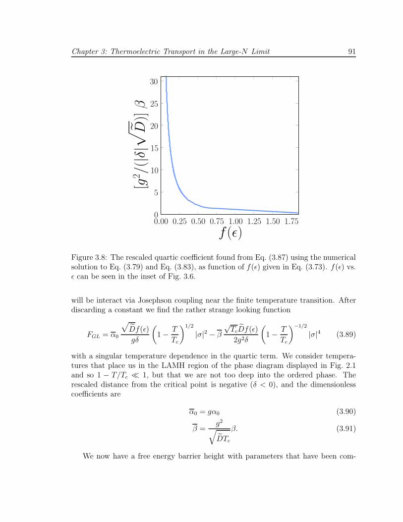
Chapter 3: Thermoelectric Transport in the Large-N Limit 91
0.00 0.25 0.50 0.75 1.00 1.25 1.50 1.75
f(ε)
0
5
10
15
20
25
30
[g2 /
(|δ|√
D)]
β
Figure 3.8: The rescaled quartic coefficient found from Eq. (3.87) using the numericalsolution to Eq. (3.79) and Eq. (3.83), as function of f(ε) given in Eq. (3.73). f(ε) vs.ε can be seen in the inset of Fig. 3.6.
will be interact via Josephson coupling near the finite temperature transition. Afterdiscarding a constant we find the rather strange looking function
FGL = α0
√Df(ε)
gδ
(1−
T
Tc
)1/2
|σ|2 − β√
TcDf(ε)
2g2δ
(1−
T
Tc
)−1/2
|σ|4 (3.89)
with a singular temperature dependence in the quartic term. We consider tempera-tures that place us in the LAMH region of the phase diagram displayed in Fig. 2.1and so 1 − T/Tc * 1, but that we are not too deep into the ordered phase. Therescaled distance from the critical point is negative (δ < 0), and the dimensionlesscoefficients are
α0 = gα0 (3.90)
β =g2
√DTc
β. (3.91)
We now have a free energy barrier height with parameters that have been com-

Chapter 3: Thermoelectric Transport in the Large-N Limit 92
−0.8 −0.4 0.0 0.4 0.8
D1/4/√
g |σ|
0.000
0.004
0.008
0.012
0.016
√D
VG
L
δ = 0.00δ = -0.40δ = -0.60
T = 0.8Tc
Figure 3.9: The Ginzburg-Landau potential of Eq. (3.77) for δ = 0.0,−0.4,−0.6 usingthe values of Tc, α0 and β found for f(ε) = π2 at T = 0.8Tc.
puted directly from the non-linear sigma model version of the full quantum theory,
∆F = −α2
2β
= −α2
0
2β
f(ε)T 3/2c
δ
(1−
T
Tc
)3/2
= −Tc
√2πf 3(ε)
4(1 + ε)3
(√Tc
δ
)3(1−
T
Tc
)3/2
×
π(1+ε)
f(ε)δ2
Tc+ 4[
(1+ε)δf(ε)
√2πTc
]4ψ(1)
[(1+ε)2δ2
f2(ε)2πTc
]− 1
2
c2(ε)− (1+ε)δf(ε)
√2πTcψ(1)
[(1+ε)2δ2
f2(ε)2πTc
] (3.92)
which can be written in terms of a dimensionless scaling function of two unique scalingvariables, the first expressing the classical and the second the quantum nature of thebarrier height
∆F = TcΦ∆F
(T
Tc,δ√Tc
). (3.93)
∆F can now be directly inserted into the LAMH theory in place of the phase slip

Chapter 3: Thermoelectric Transport in the Large-N Limit 93
0.0 0.2 0.4 0.6 0.8 1.0
|δ|/√
Tc
0.015
0.020
0.025
0.030
0.035
Φ∆
F(0
.8,δ
/√T
c)
T = 0.8Tc
Figure 3.10: The dimensionless free energy barrier height corresponding to Eq. (3.89)as a function of a single scaling variable δ/
√Tc.
barrier height calculated by Langer and Ambegaokar, with the rest of the argumentsleading to the LAMH resistance remaining unaffected.
Before this is done, we remark on the seemingly sneaky way in which we havewritten Eq. (3.93). The ability to write the barrier height as a cutoff independentscaling function with no explicit dependence on Λ or f(ε) is due to the fact that byfixing the dimensionless variable δ/
√Tc a unique value of ε and thus f(ε) can be found
from Eq (3.79). This is demonstrated in Fig. 3.10 where it appears that Φ∆F is nearlya linear function of δ/
√Tc, with a slight kink for T = 0.8Tc. Therefore, using the
same method as discussed in Section 3.1.1 we can write the quantum renormalizedLAMH conductivity in terms of the scaling function Φ∆F as
σQRLAMH = 4πe2
h
√!D
kBTc
f(ε)
c1(ε)√
Φ∆F (δ/√
Tc)
(T
Tc
)3/2(1−
T
Tc
)−3/2
× exp
[Φ∆F
(δ√Tc
)Tc
T
]. (3.94)
By the same argument given above for the cutoff independence of Φ∆F and equatingthe thermal length with the wires length at Tc (which is suitable for the crossover

Chapter 3: Thermoelectric Transport in the Large-N Limit 94
0.00 0.04 0.08 0.12 0.16
T/Tc
10−1
100
101
102
103
104
105
106
ΦQ
RLA
MH
δ/√
Tc = -1.25
δ/√
Tc = -0.50
δ/√
Tc = -0.25
Figure 3.11: The quantum renormalized LAMH scaling function for the conductiv-ity plotted as a function of the reduced temperature for three values of δ/
√Tc =
−1.25,−0.5,−0.25.
behavior expected here at finite temperatures) we have
σQRLAMH = Le2
hΦQRLAMH
(T
Tc,δ√Tc
)(3.95)
where ΦQRLAMH is shown in Fig. 3.11. The arguments discussed in Section 2.5.1provide a recipe to convert the parameter δ to the physical pair-breaking frequency αfor a given experimental geometry. The suppression of the critical temperature as aresult of an external magnetic field directed parallel to the wire has been observed inRef. [44]. Thus, in principle, the relationship between δ and Tc could be determinedexperimentally from a fitting procedure, and the expression for the conductivity inEq. (3.95) could be applied to the experimental transport results with one less fittingparameter than the form currently used in Eq. (3.3).
3.4 Large-N expansion
At low temperatures, away from the quantum critical point (√
T * δ), quantumfluctuations are large and we may now have finite Matsubara frequencies which lie
Chapter 3: Thermoelectric Transport in the Large-N Limit 95
within the gap. Thus the classical model of Section 3.2.1 is not an adequate descrip-tion of superconducting fluctuations. In this regime of the phase diagram we mayhowever use the direct 1/N expansion on the full quantum theory. Starting withthe effective action Eq. (3.5) and decoupling the quartic interaction with a Hubbard-Stratonovich field µ we arrive at the effective action
S =
∫dx
∫dτ
[D|∂xΨa(x, τ)|2 + iµ(x, τ)|Ψa(x, τ)|2 +
1
2uµ2(x, τ) + i
α
uµ(x, τ)
]
+ T∑
ωn
∫dx |ωn||Ψa(x,ωn)|2. (3.96)
Integrating out Ψa over its now quadratic action, we as usual recognize an over-all factor of N which allows us to perform the functional integral of the Hubbard-Stratonovich field µ in the saddle point approximation where we identify R = iµ. Inthe universal limit we arrive at the new quadratic effective action
SR =
∫dk
2πT∑
ωn
Ψ∗a(k,ωn)(Dk2 + |ωn| + R)Ψa(k,ωn), (3.97)
where the ‘mass’ R is defined by the saddle point condition
1
g=
∫dk
2πT∑
ωn
1
Dk2 + |ωn| + R. (3.98)
The evaluation of R is straightforward and follows our derivation of Eq (3.24)
δ√T
=
∫dk
2π2
[ln
(2π
k2
)+ ψ
(1 +
k2 + R/T
2π
)−
π
k2 + R/T
]. (3.99)
In general, this expression must be inverted numerically to determine R/T as a func-tion of δ/
√T as is shown in Fig. 3.12. However, at the quantum critical point (QC,
δ = 0) and in the metallic (M,δ → ∞) and superconducting (SC, δ → −∞) we cananalyze Eq. (3.99) along the same lines as was done for Eq. (3.24) in Section 3.2.1.We write R = TΦR(δ/
√T ) and find the following results
ΦR(x) +
1/4x2 ; x→ −∞0.625 ; x* 1π2x2 ; x→∞
. (3.100)
Understanding the behavior of the effective mass will be crucial in the followingsections where we first define and then calculate the thermal and electrical transportcoefficients in the zero frequency limit.

Chapter 3: Thermoelectric Transport in the Large-N Limit 96
−15 −10 −5 0 5 10 15
δ/√
T
10−3
10−2
10−1
100
101
102
103
104
R/T
superconductormetal
Figure 3.12: The renormalized mass R plotted as a function of the rescaled distancefrom criticality δ/
√T . The symbols refer to the analytic results of Eq. (3.100) in the
metallic and superconducting limits.
3.4.1 Thermoelectric transport
The electrical (σ) and thermal (κ) conductivities and the Peltier coefficient (α) aredefined in terms of the electrical j0 and thermal j2 current densities via the relation
(j0
j2
)=
(σ ααT κ
)(E−∇T
), (3.101)
where E is an external electric field, ∇T is an imposed temperature gradient andκ/T = κ/T − α2/σ. The current operators can also be defined in terms of thederivatives of our large-N action SR
j0 =∂SR
∂A0(3.102a)
j2 =∂SR
∂A2(3.102b)
where A0 is the scalar electric potential and A2 is the thermal vector potential, afterwe have made it gauge-covariant through the introduction of these two gauge fields[119] via the replacement
∂x → D ≡ ∂x − ie∗A0(x, τ)− iA2(x, τ)(i∂τ ) (3.103)

Chapter 3: Thermoelectric Transport in the Large-N Limit 97
leading to
j0 = ie∗D [ψ∗Dψ − ψ(Dψ)∗] (3.104)
j2 = D [∂τψ(Dψ)∗ + Dψ∂τψ∗] . (3.105)
where e∗ = 2e is the charge of a Cooper pair.We now employ the quantum Kubo formula [114, 120], to obtain results for the
thermoelectric conductivities at external frequency iωn (where we ignore the Peltiercoefficient as its dc part will turn out to be identically zero)
Gp(iωn) = −1
ωnT p
∂
∂Ap
⟨∂S
∂Ap
⟩∣∣∣∣A0=A2=0
= −1
ωnT p
β∫
0
dτ〈Jp(τ)Jp(0)〉eiωnτ − 2e∗2−pD
∫dx⟨∣∣∂p/2
τ ψ(x, 0)∣∣2⟩
(3.106)
where the currents are defined by
Jp(τ) = ie∗1−p/2D
∫dx[∂p/2τ ψ∗(x, τ)∂xψ(x, τ)− (−1)p/2∂xψ
∗(x, τ)∂p/2τ ψ(x, τ)
]
(3.107)and p = 0 corresponds to the electrical conductivity while p = 2 defines the thermalconductivity, i.e. σ(iωn) = G0(iωn) and κ(iωn)/T = G2(iωn).
We express the conductivities in terms of a one-loop polarization function,
Gp(iωn) = −4D2e∗2−p
ωnT pKp(iωn) (3.108)
which contains both paramagnetic and diamagnetic contributions
Kp(iωn) = −
= T∑
εn
∫dk
2πk2(εn +
ωn
2
)p[
1
(|ωn| + Dk2 + R)(|ωn + εn| + Dk2 + R)
−1
(|ωn| + Dk2 + R)2
]
, (3.109)
where a solid line represents the bare propagator G0(k,ωn) = (Dk2 + |ωn| + R)−1,an open circle corresponds to a term linear in the potential Ap and an open square

Chapter 3: Thermoelectric Transport in the Large-N Limit 98
to a term quadratic in Ap. We will employ the spectral representation for the barepropagator
A(k,ω) = −2Im G0(k, iωn → ω + iη)
= −2ω
ω2 + (Dk2 + R)2(3.110)
where a |ωn| dependence along the imaginary frequency axis becomes −iω just abovethe real frequency axis. The polarization function is then given by
Kp(iωn) = T∑
εn
∫dk
2πk2
∫dω1
2π
∫dω2
2π
(ω1 + ω2
2
)p
A(k,ω1)A(k,ω2)
×[
1
(iεn − ω1)(i(εn + ωn)− ω2)−
1
(iεn − ω1)(iεn − ω2)
], (3.111)
where we have made the replacement (εn + ωn/2) → (ω1 + ω2)/2, due to the tem-poral non-locality of j2 [119, 121]. Performing the Matsubara sum, and analyticallycontinuing to real frequencies yields
Kp(ω + iε) =
∫dk
2π
∫dω1
2π
∫dω2
2π
(ω1 + ω2
2
)p
A(k,ω1)A(k,ω2)k2
× [n(ω1)− n(ω2)]
(1
ω2 − ω1 − ω − iη−
1
ω2 − ω1
), (3.112)
where
n(ω) =1
eω/T − 1(3.113)
is the Bose distribution function, and η is a positive infinitesimal. After checkingthat the delta-function contribution to ReGp(ω) at zero frequency is proportional tothe external frequency, i.e. it vanishes as ω → 0, we can combine Eqs. (3.108) and(3.112) to give the remaining regular part
ReGp(ω) =4D2e∗2−p
T p
∫dΩ
π
[n(Ω)− n(Ω + ω)]
ω
(Ω +
ω
2
)p
×∫
dk
2π
k2Ω(Ω + ω)
[Ω2 + (Dk2 + R)2][(Ω + ω)2 + (Dk2 + R)2]. (3.114)
The classical limit of Eq. (3.114) corresponding to replacing n(ω) + T/ω is examinedin Appendix A but here we directly perform the limit ω → 0 and obtain the quantumdc conductivities
ReGp =D2e∗
2−p
T p+1
∫dΩ
π
Ω2+p
sinh2(Ω/2T )
∫dk
2π
k2
[Ω2 + (Dk2 + R)2]2
=
√2e∗2−p
√D
8T p+1
∫dΩ
2π
Ω2+p
sinh2(Ω/2T )
1√Ω2 + R2
(R +
√Ω2 + R2
)3/2. (3.115)

Chapter 3: Thermoelectric Transport in the Large-N Limit 99
which is the major result of this section. From this expression it is immediately clearthat the Peltier coefficient α (corresponding to p = 1) is identically zero by symmetry,and thus κ = κ.
In addition to the scaling function Φσ defined for the electrical conductivity inEq. (3.50) and given by
σ =e∗2
!
√!D
kBTΦσ
(δ√
!kBT
)(3.116)
the thermal conductivity must obey a similar form
κ
T=
k2B
!
√!D
kBTΦκ
(δ√
!kBT
), (3.117)
where we have re-inserted the appropriate factors of ! and kB for clarity.The δ/
√T dependence of Φσ and Φκ can be found by numerically inverting
Eq. (3.99), (Fig. 3.12) and the result is shown in Fig. 3.13. We can now comparethe large-N result with the previously calculated value in Section 3.2.2 for N = 1.The quantitative agreement is not striking, but the two results have similar δ/
√T de-
pendence near δ = 0 indicating that the correct physics are manifest even at N =∞.The temperature dependence of the transport functions is found by fixing δ leadingto the results displayed in Fig. 3.14 and 3.15. The singular correction to the electri-cal conductivity clearly shows behavior consistent with a quantum phase transitionbetween a superconductor (diverging conductivity) and metal (finite or vanishing con-ductivity). Moreover, the inset shows that for a fixed value of δ which places us nottoo far into the metallic phase, as we lower the temperature a crossover can be seenfrom an increasing to decreasing conductivity. As mentioned in the introduction, ex-periments have seen evidence of such non-monotonic resistance in the metallic regime,and this strongly supports the crossover picture we have presented here.
We now attempt to quantify these crossovers by investigating the limiting formsof the two scaling functions Φσ and Φκ.
Limiting forms of σ an κ/T
We can obtain analytical estimates for the electrical and thermal conductivityin three distinct limits using the results of Eq. (3.100). The first is deep in thesuperconducting (SC) regime where δ/
√T → −∞ or R/T → 0. The next is at the
quantum critical point (QC), where δ = 0 or R/T = 0.624798 and the final regime ison the metallic side of the transition (M) where δ, R/T →∞. For low temperatures,

Chapter 3: Thermoelectric Transport in the Large-N Limit 100
−4 −3 −2 −1 0 1 2 3 4
δ/√
T
10−5
10−4
10−3
10−2
10−1
100
101
102
Φσ
N = ∞, p = 0N = 1, p = 0
−4 −3 −2 −1 0 1 2 3 40.0
0.1
0.2
0.3
0.4
0.5
0.6
0.7
Φκ
N = ∞, p = 2
Figure 3.13: The solid lines show the N = ∞ universal scaling functions the elec-trical (p = 0, left axis) and thermal (p = 2, right axis) conductivity calculated byintegration of Eq. (3.115). The symbols show the effective classical scaling functionfor the electrical conductivity calculated in the Langevin formalism in Section 3.2.2and previously shown in Fig. 3.3 for a one component complex field.
we can evaluate Eq. (3.115) in these three limits leading to
σ = e∗2
√D
T
18
(RT
)−3/2; SC
0.217997 · · · ; QCπ12
(RT
)−5/2; M
(3.118)
κ
T=
√D
T
34√
2πζ(
32
); SC
0.24592 · · · ; QCπ3
15
(RT
)−5/2; M
. (3.119)

Chapter 3: Thermoelectric Transport in the Large-N Limit 101
1 2 3 4
T
10−710−610−510−410−310−210−1100101102103104105106
σ/e
∗2√
D
δ = -0.50δ = -0.20δ = -0.10δ = 0.00δ = 0.10δ = 0.20δ = 0.50
0 1 2 3 4
T
0.00
0.04
0.08
0.12
σ/e
∗2√
D
δ = 0.10δ = 0.20δ = 0.50
Figure 3.14: The temperature dependence of dc electrical conductivity at fixed valuesof δ. The inset shows non-monotonic behavior just above the quantum critical pointdefined by δ = 0.
and using Eq. (3.100)
Φσ(x) =
x3 ; SC0.217997 · · · ; QC(12π4x5)−1 ; M
(3.120)
Φκ(x) =
34√
2πζ(
32
); SC
0.24592 · · · ; QC(15π2x5)−1 ; M
. (3.121)
The temperature dependence of these results are summarized in Table 3.1. We havenow derived the exact form of the temperature dependence describing the crossoverbehavior, with the conductivity increasing like 1/
√T at high temperatures while
the system is in the quantum critical regime of Fig. 2.1 and finally decreasing asT 2 after we have fully returned to metallic behavior. Although we are about toshow that a microscopic theory reproduces the T 2 metallic conduction, the 1/
√T
dependence of the conductivity is not present in the simple Gaussian theory and anaccurate determination of the full crossover phase diagram necessitates the inclusionof interactions between Cooper pairs.
We now comment on a shared regime of validity between our large-N theory andthe disordered electron perturbation theory of Ref. [83]. A closer investigation of the

Chapter 3: Thermoelectric Transport in the Large-N Limit 102
1 2 3 4T
0.0
0.5
1.0
1.5
2.0
(κ/T
)/√
Dδ = -0.50δ = -0.20δ = -0.10δ = 0.00δ = 0.10δ = 0.20δ = 0.50
0 1 2 3 4
T
0.00
0.05
0.10
0.15
0.20
0.25
0.30
(κ/T
)/√
D δ = 0.10δ = 0.20δ = 0.50
Figure 3.15: The temperature dependence of dc electrical conductivity at fixed valuesof δ. The inset shows non-monotonic behavior just above the quantum critical pointdefined by δ = 0.
dc electrical conductivity in the metallic regime with careful attention to all prefactorsyields
σ =e∗2
!
π√
DT 2
12R5/2. (3.122)
We note that upon comparing the large-N propagator of Eq. (3.98) with Eq. (4) ofRef. [83] that our mass R is exactly double the mass α employed by Lopatin et al.,i.e. R = 2[α− αc(T )]. Having made this identification, we may compare Eq. (3.122)above, with the finite temperature fluctuation correction to the normal state con-ductivity computed via diagrammatic perturbation theory (Eq. (8) in Ref. [83]), andfind exact agreement. After a rather lengthy calculation it was confirmed that per-fect correspondence is also found for the thermal conductivity in this limit [96]. Theconcurrence between the two theoretical approaches in this limit is a result of anapproximation made in the diagrammatic calculation involving an infinite sum over aclass of ladder diagrams which turns out to be equivalent to the large-N limit takenhere.
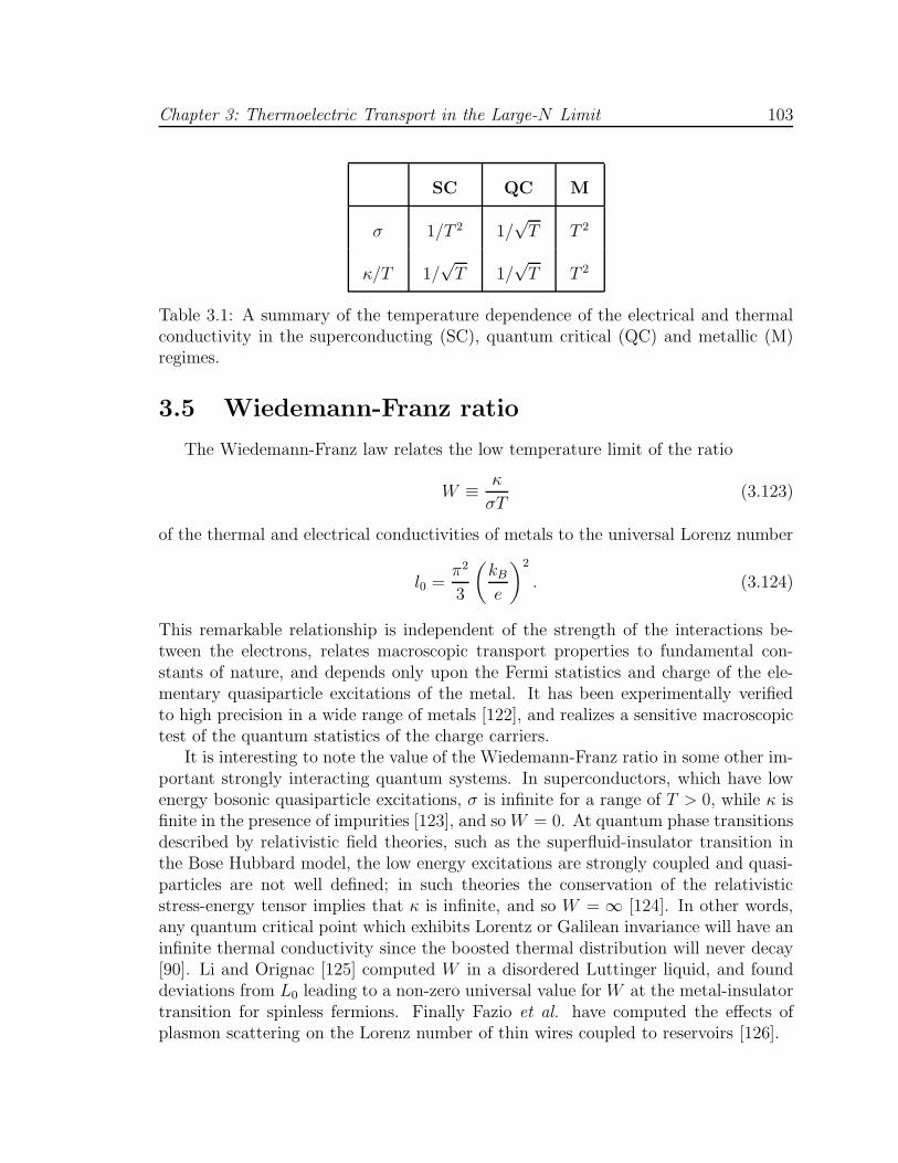
Chapter 3: Thermoelectric Transport in the Large-N Limit 103
SC QC M
σ 1/T 2 1/√
T T 2
κ/T 1/√
T 1/√
T T 2
Table 3.1: A summary of the temperature dependence of the electrical and thermalconductivity in the superconducting (SC), quantum critical (QC) and metallic (M)regimes.
3.5 Wiedemann-Franz ratio
The Wiedemann-Franz law relates the low temperature limit of the ratio
W ≡κ
σT(3.123)
of the thermal and electrical conductivities of metals to the universal Lorenz number
l0 =π2
3
(kB
e
)2
. (3.124)
This remarkable relationship is independent of the strength of the interactions be-tween the electrons, relates macroscopic transport properties to fundamental con-stants of nature, and depends only upon the Fermi statistics and charge of the ele-mentary quasiparticle excitations of the metal. It has been experimentally verifiedto high precision in a wide range of metals [122], and realizes a sensitive macroscopictest of the quantum statistics of the charge carriers.
It is interesting to note the value of the Wiedemann-Franz ratio in some other im-portant strongly interacting quantum systems. In superconductors, which have lowenergy bosonic quasiparticle excitations, σ is infinite for a range of T > 0, while κ isfinite in the presence of impurities [123], and so W = 0. At quantum phase transitionsdescribed by relativistic field theories, such as the superfluid-insulator transition inthe Bose Hubbard model, the low energy excitations are strongly coupled and quasi-particles are not well defined; in such theories the conservation of the relativisticstress-energy tensor implies that κ is infinite, and so W = ∞ [124]. In other words,any quantum critical point which exhibits Lorentz or Galilean invariance will have aninfinite thermal conductivity since the boosted thermal distribution will never decay[90]. Li and Orignac [125] computed W in a disordered Luttinger liquid, and founddeviations from L0 leading to a non-zero universal value for W at the metal-insulatortransition for spinless fermions. Finally Fazio et al. have computed the effects ofplasmon scattering on the Lorenz number of thin wires coupled to reservoirs [126].
Chapter 3: Thermoelectric Transport in the Large-N Limit 104
Upon examination of Table 3.1 it can immediately be seen that the Wiedemann-Franz ratio is temperature independent in both the quantum critical and metallicregimes. Remarkably, all important couplings between bosons and fermions scale touniversal values, and consequently, by studying equations (3.118) and (3.119) we findthe universal constant
WQC = (0.28203 · · · )(
kB
e
)2
(3.125)
in the quantum critical regime whereas in the metallic region of the phase diagram
WM =π2
5
(kB
e
)2
. (3.126)
Both of these corrections are smaller than the Lorenz number and thus it appearsthat the Cooper pairs tend to carry more charge than heat.
These results for the Wiedemann-Franz ratio conclude this chapter, but in thenext chapter we will extend the theory presented here for N = ∞ to the first orderin 1/N . We will exploit the anomalous scaling dimension of the dynamical criticalexponent z to find additional universal corrections to Eq. (3.125).

Chapter 4
1/N Corrections to Transport
This chapter is quite heavy on calculational details and can be skipped by thecasual reader. The main results include the derivation of a critical theory for a finiteN component complex field Ψa governing the fluctuations of Cooper pairs near asuperconductor-metal transition. This theory is used to systematically compute the1/N corrections to critical exponents and the zero frequency transport coefficientscalculated in the previous chapter at N = ∞ when the coupling parameter whichdrives the SMT attains its critical value. We will find (Eq. (4.86)) that although theindividual values of the electrical and thermal conductivities are not universal, butdepend explicitly on an ultra-violet cutoff, their Wiedemann-Franz ratio is a pure,temperature independent universal number proportional to 1/N that characterizesthe most singular corrections to transport in the strongly fluctuating quantum criticalregime
W =
(0.282 +
0.0376
N
)(kB
e
)2
. (4.1)
4.1 The critical theory
We begin by reintroducing the strong-coupling effective action of Eq. (3.11) foran N -component Cooper pair operator Ψa
Sg =1
gT∑
ωn
∫dk
2π(k2 + |ωn|)|Ψa(k,ωn)|2 (4.2)
where we have chosen to rescale distances by a factor of the square root of the effectivediffusion constant D and must enforce the “hard spin” constraint |Ψ(x, τ)|2 = 1.Imposing the delta-function constraint via a Lagrange multiplier µ and performing a
105

Chapter 4: 1/N Corrections to Transport 106
rescaling of the field Ψa →√
gΨa we have the partition function
Z =
∫DΨaDΨ∗
aDµ exp
−∫
dx
∫dτ
[Ψ∗
a(x, τ)(−∂2
x + |∂τ | + iµ(x, τ))Ψa(x, τ)
−N
giµ(x, τ)
], (4.3)
where we have again used the notation |∂τ | to infer |ωn| after Fourier transforming.Integrating out the Ψa fields, we are left with
Z =
∫Dµ exp
−N
[Tr ln
(−∂2
x + |∂τ | + iµ(x, τ))−
i
g
∫dx
∫dτµ(x, τ)
](4.4)
and as previously, for N large, we can approximate the functional integral over µ byits saddle point value defined to be r = iµ leading to
1
g= T
∑
ωn
∫dk
2π
1
k2 + |ωn| + r. (4.5)
This is an auspicious point to make a brief comment regarding the relationship be-tween the notation introduced here and that of the previous chapter. Eq. (4.5) isidentical to Eq. (3.98) with the replacement of r → R. However, in this chapter,unless otherwise stated, we will be considering a critical theory (whether at zero orfinite temperatures) with the coupling g equal to its critical value gc which will beshifted from its N = ∞ value by a correction of order 1/N . As a result, the effectivemass r will be also corrected from its N = ∞ saddle point value. This will be mademore explicit soon, but for now we simply indicate that r = R+O(1/N) with R equalto its N = ∞ value defined by Eq. (3.98) with g = gc.
Let us now look at fluctuations around the saddle point by defining iµ = r+iλ, andafter expanding to quadratic order in λ and noticing that with the help of Eq. (4.5)all linear terms cancel we have
Z =
∫Dλ exp
−N
[
Tr ln(−∂2x + |∂τ | + r) +
1
2
∑
ωn
∫dk
2πλ2ΠT (k,ωn, r)
]
(4.6)
where
ΠT (k,ωn, r) = T∑
εn
∫dq
2π
1
[(k + q)2 + |ωn + εn| + r](q2 + |εn| + r)(4.7)
can be thought of as the propagator for a λ field leading to 1/N fluctuations.Upon examination of Eq. (4.6), we observe that we could have simply started from
a partition function for our original field Ψa with an additional interaction term such

Chapter 4: 1/N Corrections to Transport 107
that its diagrammatic expansion is equivalent to that of Eq. (4.6), i.e.
Z =
∫DΨaDΨ∗
aDλ exp
−∫
dx
∫dτ
[Ψ∗
a(x, τ)(−∂2
x + |∂τ | + r)Ψa(x, τ)
+ iλ(x, τ)|Ψa(x, τ)|2 +N
2
∫dx′∫
dτ ′λ(x, τ)ΠT (x− x′, τ − τ ′, r)λ(x′, τ ′)
]
(4.8)
leading to the effective action in momentum space
Sr = T∑
ωn
∫dk
2π
[(k2 + |ωn| + r)|Ψa(k,ωn)|2 +
N
2|λ(k,ωn)|2ΠT (k,ωn, r)
+ T∑
εn
∫dq
2πΨ∗
a(k,ωn)Ψa(q, εn)λ(k − q,ωn − εn)
] (4.9)
where we note that in order to avoid double-counting, the λ or fluctuation propagatorΠT cannot have a self-energy contribution of a single Ψa bubble (since it has alreadybeen included). Thus, performing a direct 1/N expansion from Z for G(k,ωn) =〈|Ψa(k,ωn)|2〉 [48] we have
G(k,ωn) = + + + · · · (4.10)
where a solid line is equal to (k2 + |ωn| + r)−1, a dashed line equal to ΠT /N and asolid dot represents the interaction vertex i. There is no tadpole graph as it is alreadyincluded in the 1/N correction to the effective mass r. The third graph has two loops,but is only of order 1/N as we any closed Ψa loop gives a factor of N . Combiningthese graphs leads to
G−1(k,ωn) = k2 + |ωn| + r +1
NT∑
εn
∫dq
2π
1
ΠT (q, εn, r)
1
((k + q)2 + |ωn + εn| + r)
−1
N
1
ΠT (0, 0, r)T∑
εn
∫dq
2πT∑
νn
∫dp
2π
1
ΠT (q, εn, r)
×1
(p2 + |νn| + r)2[(p + q)2 + |εn + νn| + r]. (4.11)
4.1.1 Critical point at T = 0
Now let us determine the value of the critical coupling gc to order 1/N at T = 0.At T = 0, the critical point is determined by the condition G−1(0, 0) = 0, r = rc. So
Chapter 4: 1/N Corrections to Transport 108
keeping terms only up to order 1/N
rc = −1
N
∫dk
2π
∫dω
2π
1
Π0(k,ω, 0)
1
k2 + |ω|
+1
N
1
Π0(0, 0, 0)
∫dk
2π
∫dω
2π
∫dq
2π
∫dε
2π
1
(k2 + |ω|)2[(k + q)2 + |ω + ε|]1
Π0(q, ε, 0)(4.12)
where
Π0(k,ω, 0) =
∫dq
2π
∫dε
2π
1
(q2 + |ε|)[(k + q)2 + |ω + ε|]
=1
4π|k|
[2 arcsin
(k2 − |ω|k2 + |ω|
)+ π
](4.13)
+1
4π√
k2 + 2|ω|ln
(2√
|ω|√
k2 + 2|ω|+ k2 + 3|ω||2√|ω|√
k2 + 2|ω|− k2 − 3|ω||
)
(4.14)
with details given in Appendix B. Note that Π0(0, 0, 0) is infrared divergent, butthis will shortly cancel out of observable quantities. Inserting the expansion for rc inEq. (4.5), we obtain
1
gc=
∫dk
2π
∫dω
2π
1
k2 + |ω|+
Π0(0, 0, 0)
N
∫dk
2π
∫dω
2π
1
Π0(k,ω, 0)
1
k2 + |ω|
−1
N
∫dk
2π
∫dω
2π
∫dq
2π
∫dε
2π
1
(k2 + |ω|)2[(k + q)2 + |ω + ε|]1
Π0(q, ε, 0)
=
∫dk
2π
∫dω
2π
1
k2 + |ω|+
1
N
∫dk
2π
∫dω
2π
∫dq
2π
∫dε
2π
1
Π0(q, ε, 0)(k2 + |ω|)2
×[
1
q2 + |ε|−
1
(k + q)2 + |ω + ε|
](4.15)
which is free of infrared divergences.
4.1.2 Quantum critical propagator
Now let us move to T > 0 at g = gc where we write r = R+R1 with R1 ∼ O(1/N).As mentioned previously, R is determined by setting r = R in Eq. (4.5) when g = gc
takes its N = ∞ value
T∑
ωn
∫dk
2π
1
k2 + |ωn| + R=
∫dk
2π
∫dω
2π
1
k2 + |ω|. (4.16)
We have seen this equation before in Eq. (3.98) with g = gc and can thus express it asEq. (3.99) with δ = 0 giving an equation that can be inverted to uniquely determine

Chapter 4: 1/N Corrections to Transport 109
R/T ,
0 =
∫dk
2π
[πT
k2 + R− ψ
(1 +
k2 + R
2πT
)+ ln
(k2
2πT
)](4.17)
where ψ(x) is the polygamma function. Solving numerically we find
R
T+ 0.624798. (4.18)
Now, returning to Eq. (4.5) we can write (to order 1/N)
1
gc= T
∑
ωn
∫dk
2π
1
k2 + |ωn| + R + R1
= T∑
ωn
∫dk
2π
1
k2 + |ωn| + R− ΠT (0, 0, R)R1 (4.19)
which can be compared with our expression for 1/gc in Eq. (4.15) order by order toyield
R1 = −1
NΠT (0, 0, R)
∫dk
2π
∫dω
2π
∫dq
2π
∫dε
2π
1
(k2 + |ω|)2
1
Π0(q, ε, 0)
×[
1
q2 + |ε|−
1
(k + q)2 + |ω + ε|
](4.20)
and note that√
T ΠT (0, 0, R) is a finite universal number given by (see Appendix B)
√T ΠT (0, 0, R) =
1
4(2π)3/2
[ζ
(3
2,
R
2πT
)+ ζ
(3
2,
R
2πT+ 1
)], (4.21)
where ζ(m, x) is the Hurwitz Zeta function.Inserting everything in Eq. (4.11) we write
G−1(k,ωn) = k2 + |ωn| + R + R1 + Σ(k,ωn) (4.22)
where the self energy Σ(k,ωn) is defined to be
Σ(k,ωn) =1
NT∑
εn
∫dq
2π
1
ΠT (q, εn, R)
[1
(k + q)2 + |ωn + εn| + R−
1
q2 + |εn| + R
]
(4.23)such that Σ(0, 0) = 0, and
R1 = −1
NΠT (0, 0, R)
∫dk
2π
∫dω
2π
∫dq
2π
∫dε
2π
1
(k2 + |ω|)2
1
Π0(q, ε, 0)
×[
1
q2 + |ε|−
1
(k + q)2 + |ω + ε|
]
−1
ΠT (0, 0, R)T∑
ωn
∫dk
2π
1
(k2 + |ωn| + R)2Σ(k,ωn). (4.24)

Chapter 4: 1/N Corrections to Transport 110
This is equivalent to Eq. (4.6) in Ref. [127]. It will be useful to interchange the ordersof integration in both terms and write
R1 =1
NΠT (0, 0, R)
−∫
dq
2π
∫dε
2π
1
Π0(q, ε, 0)
∫dk
2π
∫dω
2π
1
(k2 + |ω|)2
×[
1
q2 + |ε|−
1
(k + q)2 + |ω + ε|
]
+ T∑
εn
∫dq
2π
1
ΠT (q, ε, R)T∑
ωn
∫dk
2π
1
(k2 + |ωn| + R)2
×[
1
(q2 + |εn| + R)−
1
(k + q)2 + |ωn + εn| + R)
]. (4.25)
Now, both the inner integral or sum over (k,ω) and (k,ωn) is ultraviolet convergent,but the outer integral appears to be divergent. We carefully re-arrange the integralas follows (where we now explicitly indicate the integration bounds)
R1 =1
NΠT (0, 0, R)
−
Λ2∫
−Λ2
dω
2π
Λ∫
−Λ
dk
2π
1
Π0(k,ω, 0)
×∞∫
−∞
dq
2π
∞∫
−∞
dε
2π
1
(q2 + |ε|)2
[1
k2 + |ω|−
1
(k + q)2 + |ω + ε|
]
+ T∑
|ωn|<Λ2
Λ∫
−Λ
dk
2π
1
ΠT (k,ωn, R)
[ΠT (0, 0, R)
k2 + |ωn| + R+
1
2
∂ΠT (k,ωn, R)
∂R
]
, (4.26)
where Λ is an ultra-violet momentum cutoff. This expression can be evaluated nu-merically for a fixed Λ by rescaling the integration variables to be dimensionless suchthat
R1
T=
1
N
8√
2π3/2
ζ(3/2, R/2πT ) + ζ(3/2, R/2πT + 1)
×
−
Λ2/T∫
−Λ2/T
dω
2π
Λ/√
T∫
−Λ/√
T
dk
2π
1
Π0(k,ω, 0)
∞∫
−∞
dq
2π
∞∫
−∞
dε
2π
1
(q2 + |ε|)2
×[
1
k2 + |ω|−
1
(k + q)2 + |ω + ε|
]+ T
∑
2π|n|<Λ2/T
Λ/√
T∫
−Λ/√
T
dk
2π
1
ΠT (k, 2πn, R/T )
×[ζ(3/2, R/2πT ) + ζ(3/2, R/2πT + 1)
(8√
2π3/2)(k2 + 2π|n| + R/T )+
1
2
∂ΠT (k, 2πn, R/T )
∂(R/T )
]
. (4.27)

Chapter 4: 1/N Corrections to Transport 111
0.00 0.02 0.04 0.06 0.08√T/Λ
0.100
0.102
0.104
0.106
0.108
0.110
0.112
NR
1/T
R1T
∣∣Λ→∞ ' 0.1069
N
Figure 4.1: The behavior of Eq. (4.27) as the UV cutoff Λ → ∞. When fit to aquadratic polynomial in
√T/Λ it converges to the value R1/T + 0.1069/N .
Using Eq. (4.18), we find that R1/T converges to the universal finite value
R1
T+
0.1069
N(4.28)
as seen in in Fig. 4.1. Therefore, as described in Ref. [99] and Section 2.2 as aconsequence of the scaling relation z = 2− η where η is the anomalous dimension ofΨa, the uniform static order parameter susceptibility
χ =
∫dx
∫dτ〈Ψ∗
a(x, τ)Ψa(0, 0)〉 (4.29)
is determined by the value of kBT alone using Eqs. (4.18) and (4.22) as
χ−1 = kBT
(0.6248 +
0.107
N
). (4.30)
4.2 Critical exponents
With our quantum critical theory firmly established, we may now investigate anypossible 1/N corrections to the large-N critical behavior characterized by exponents

Chapter 4: 1/N Corrections to Transport 112
z = 2 and ν = 1. Such corrections can be obtained by exploiting the known scalingbehavior of the susceptibility in conjunction with various hyperscaling relations. Webegin by computing the anomalous dynamical scaling dimension η which corrects zat order 1/N .
Evaluation of η
We know that the susceptibility should scale with momentum like G−1(k, 0) = kz
where the bare dynamical critical exponent z = 2 will be corrected by the criticalexponent η as z = 2− η. Therefore, we can write
G−1(k, 0) = k2−η
= k2
(1 + η ln
Λ
k
)(4.31)
where Λ is a large momentum cutoff. From Eq. (4.11) at r = rc, T = 0 and ω = 0 wehave
G−1(k, 0) = k2 +1
N
∫dq
2π
∫dε
2π
1
Π0(q, ε, 0)
[1
(k + q)2 + |ω + ε|−
1
q2 + ε
](4.32)
and thus we need only extract the log divergence in the above equation. UsingEq. (B.5) and rescaling such that all variables of integration are dimensionless wehave
G−1(k, 0) = k2 +k2
N
Λ/k∫
−Λ/k
dq
2π|q|
∞∫
0
dε
π
1
Π0(1, ε, 0)
[1
(1 + 1/q)2 + ε−
1
1 + ε
]. (4.33)
Expanding the integrand for large q and identifying the logarithmic prefactor leadsto
η =1
π2N
∞∫
0
dε3− ε
Π0(1, ε, 0)(ε+ 1)3
+0.13106
N. (4.34)
Knowing the value of η will be particularly useful because it will fix the cutoff de-pendence of the quantum critical conductivity at order 1/N , since z = 2− η, and weexpect σ(T ) ∼ T−1/z. Thus, if σ(T ) = A/
√T where A is a constant at N = ∞, then
at order 1/N we should have σ = (A/√
T )[1 + (η/2) ln(Λ/√
T )].

Chapter 4: 1/N Corrections to Transport 113
Evaluation of ν
Calculating the 1/N correction to the correlation length exponent ν is unfortu-nately not so simple, but we begin by examining the behavior of the inverse sus-ceptibility at T = 0 and k = ω = 0 as one tunes the coupling constant g towardsgc
G−1(0, 0) ∼ (g − gc)γ (4.35)
which defines the susceptibility exponent γ. At N =∞ we know γ = 2, and thus forfinite N let us parameterize γ = 2(1− α), which can be related to ν via the scalingrelation γ = (2− η)ν. To this end, let us define rg via
1
gc−
1
g≡∫
dk
2π
∫dω
2π
(1
k2 + |ω|−
1
k2 + |ω|+ rg
)
=
√rg
π, (4.36)
where we have exploited the fact that
√rg =
1
2πΠ0(0, 0, rg). (4.37)
Thus, from Eq. (4.36) we have rg ∼ (g − gc)2, and upon comparison with Eq. (4.35)we find
G−1(0, 0) = (g − gc)2(1−α)
= r1−αg
= rg
(1 + α ln
Λ2
rg
). (4.38)
So again we can extract a critical exponent by determining the prefactor of a log-arithmic divergence of G−1. At this stage it will useful to quote the following tworesults (with details given in Appendix B)
Π0(k,ω, r) =1
2π|k|
[
asin
(k2 + |ω|
√(k2 + |ω|)2 + 4k2r
)
+ asin
(k2 − |ω|
√(k2 + |ω|)2 + 4k2r
)]
+1
4π√
k2 + 2|ω| + 4r
[
ln
(2√
r + |ω|√
k2 + 2|ω| + 4r + k2 + 3|ω|+ 4r
|2√
r + |ω|√
k2 + 2|ω|+ 4r − k2 − 3|ω|− 4r|
)
− ln
(2√
r√
k2 + 2|ω| + 4r + k2 + |ω| + 4r
|2√
r + |ω|√
k2 + 2|ω| + 4r − k2 − |ω|− 4r|
)]
(4.39)
and
Π′0(k,ω, r) ≡
∂Π0(k,ω, r)
∂r= −2
∫dq
2π
∫dε
2π
1
(q2 + |ε| + r)2[(k + q)2 + |ω + ε| + r].
(4.40)
Chapter 4: 1/N Corrections to Transport 114
Combining Eqs. (4.5) with (4.15) and (4.36) we can write
r = rg −2π√
rg
N
∫dk
2π
∫dω
2π
∫dq
2π
∫dε
2π
1
(k2 + |ω|)2
1
Π0(q, ε, 0)
×(
1
q2 + |ε|−
1
(k + q)2 + |ω + ε|
). (4.41)
Now using Eq. (4.11) and (4.41), we have the result for the inverse susceptibility
G−1(0, 0) = rg +1
N
∫dk
2π
∫dω
2π
1
Π0(k,ω, rg)
1
(k2 + |ω| + rg)
−1
N
1
Π0(0, 0, rg)
∫dk
2π
∫dω
2π
∫dq
2π
∫dε
2π
×
1
Π0(q, ε, rg)
1
(k2 + |ω| + rg)2[(k + q)2 + |ω + ε| + rg]
+1
Π0(q, ε, 0)
1
(k2 + |ω|)2
[1
q2 + |ε|−
1
(k + q)2 + |ω + ε|
](4.42)
where we have been able to replace r with rg in any term that is already of order1/N . A useful check is to note that G−1(0, 0) = 0 above for rg = 0. Let us now writethis result in the form
G−1(0, 0) = rg + F (rg)−2π√
rg
N
∫dk
2π
∫dω
2π
∫dq
2π
∫dε
2π
1
Π0(q, ε, 0)
×1
(k2 + |ω|)2
[1
q2 + ε−
1
(k + q)2 + |ω + ε|
](4.43)
where
F (rg) =1
N
∫dk
2π
∫dω
2π
1
Π0(k,ω, rg)
[1
k2 + |ω| + rg+
Π′0(k,ω, rg)
2Π0(0, 0, rg).
](4.44)
The next step is to find the small rg behavior of F (rg). For this, let us first examinethe small rg behavior of Π′
0:
Π′0(k,ω, rg) = −2
∫dq
2π
∫dε
2π
1
(q2 + |ε| + rg)2[(k + q)2 + |ω + ε| + rg]
= −1
π(k2 + |ω|)√rg+ C1(k,ω) + C2(k,ω)
√rg + · · · (4.45)
where
C1(k,ω) = 2
∫dq
2π
∫dε
2π
1
(q2 + |ε|)2
[1
k2 + |ω|−
1
(k + q)2 + |ω + ε|
]
≡1
|k|3Φ1
(|ω|k2
)(4.46)

Chapter 4: 1/N Corrections to Transport 115
with
Φ1
(|ω|k2
)=
∫dq
2π
∫dε
2π
1
(q2 + |ε|)2
[1
1 + |ω|/k2−
1
(1 + q)2 + |ε+ ω/k2|
]. (4.47)
and
C2(k,ω) = − limrg→0
4√
rg
∫dq
2π
∫dε
2π
d
drg
[1
(q2 + |ε| + rg)2[(k + q)2 + |ω + ε| + rg]
−1
(k2 + |ω|)(q2 + |ε| + rg)2−
1
(q2 + |ε|)2[(k + q)2 + |ω + ε|]
+1
(q2 + |ε|)2(k2 + |ω|)
]
=3
π(k2 + |ω|)2+
3k2 − |ω|π(k2 + |ω|)3
≡1
k4Φ2
(|ω|k2
), (4.48)
with
Φ2
(|ω|k2
)=
2
π
3 + |ω|/k2
(1 + |ω|/k2)3(4.49)
where we have used the fact that |ε| * ω over the regime important for small rg.From this expansion we can also determine the small rg expansion of Π0
Π0(k,ω, rg) = Π0(k,ω, 0)−2√
rg
π(k2 + |ω|)+ C1(k,ω)rg +
2C2(k,ω)
3r3/2g + · · · (4.50)
and finally that of F (rg)
F (rg) =π√
rg
N
∫dk
2π
∫dω
2π
C1(k,ω)
Π0(k,ω, 0)+
rg
N
∫dk
2π
∫dω
2π
[2C1(k,ω)
(k2 + |ω|)Π20(k,ω, 0)
+πC2(k,ω)
Π0(k,ω, 0)−
1
(k2 + |ω|)2Π0(k,ω, 0)
]. (4.51)
Now, comparing this result with Eq. (4.38) and (4.43) the second term, which is linearin rg defines α by
F (rg) = · · ·+ αrg ln
(Λ2
rg
)+ · · · (4.52)
where α is related to the critical exponents by γ = 2(1 − α) = ν(2 − η). UsingEq. (B.5) to define
Φ0
(|ω|k2
)= |k|Π0(k,ω, 0) (4.53)

Chapter 4: 1/N Corrections to Transport 116
and via Eqs. (4.46) and (4.48), α is given by
α =1
2π2N
∞∫
0
dω
[2Φ1(ω)
(ω + 1)Φ20(ω)
+πΦ2(ω)
Φ0(ω)−
1
(1 + ω)2Φ0(ω)
]
+0.455
N. (4.54)
The value of ν can be finally determined using Eq. (4.34) as
ν = 1− α +η
2
+ 1−0.389
N. (4.55)
The values found in this section for z = 2 − η (Eq. (4.34)) and ν (Eq. (4.55))corresponding to a N component complex field are fully consistent with previouscalculations including an ε expansion near 2 dimensions [99, 89] (Eq. (2.14) and(2.15)) and via Monte Carlo simulations where z = 1.97(3) and ν = 0.689(6) [101].
4.3 Quantum transport at finite N
We now we endeavor to compute the dc values of the thermal and electrical con-ductivity in a 1/N expansion in the quantum critical regime. Transport is againcalculated via the Kubo formula, and the initial steps are identical to those presentedin Section 3.4.1 for the derivation of Eq. (3.108). However, unlike the case where thenumber of components of our order parameter field was infinite, we now have themodified propagator of Eq. (4.22) and the single polarization bubble diagrams willbe corrected by additional loops giving rise to corrections of order 1/N .
It will turn out that although the individual values of the thermal (κ) and elec-trical (σ) conductivities are not by themselves universal to order 1/N their ratio isa universal number, solely as a result of the appearance of an anomalous dimensionthat alters the critical dynamic scaling.
4.3.1 Diagrammatic expansion
We refer the reader to Eq. (3.101) to Eq. (3.108) and begin by writing down theexpression for the value of the transport coefficients (p = 0 for electrical conductivityand p = 2 for thermal conductivity) obtained from the Kubo formula in terms of apolarization function at external imaginary frequency iωn
Gp(iωn) = −4e∗2−p
ωnT pKp(iωn). (4.56)
Chapter 4: 1/N Corrections to Transport 117
Written in Fourier space it takes the form, where 〈· · · 〉 refers to an expectation valuewith respect to Sr, Eq. (4.9).
Kp(iωn) = −T
2
∑
εn
∫dk
2π(εn + ωn/2)p
[〈|ψ(k, εn)|2〉
− k2〈Ψ∗a(k, εn)Ψa(k, εn + ωn)Ψ∗
a(k, εn + ωn)Ψa(k, εn)〉].
(4.57)
As we are only interested in the dc thermal and electric transport, we will need todetermine the imaginary part of Kp, analytically continued to real frequencies. Ourprevious experience indicates that we need only focus on the paramagnetic contri-butions to Eq. (4.57) which correspond to the four-point correlation function aboveresulting from quadratic insertions of the scalar or thermal potentials Aj. The re-sulting paramagnetic polarization function has the diagrammatic expansion to order1/N given by
Kparap (iωn) = + 2 + 2 + (4.58)
= + (4.59)
where
=1
k2 + |εn| + r(4.60)
= G0(k, εn) =1
k2 + |εn| + R(4.61)
=1
k2 + |εn| + R + R1 + Σ(k, εn), (4.62)
r = R + R1 and an open circle indicates a factor of k(εn + ωn/2)p/2 where p = 0for electrical transport and p = 2 for thermal transport. R1 is the finite shift inthe critical point to order 1/N given by Eq. (4.28) and the self-energy is defined inEq. (4.23) such that Σ(0, 0) = 0. To identify the role of various 1/N corrections to

Chapter 4: 1/N Corrections to Transport 118
transport it will be useful to present the full integral form
Kparap (iωn) = T
∑
εn
∫dk
2πk2(εn + ωn/2)pG0(k, εn)G0(k, εn + ωn)
− 2R1T∑
εn
∫dk
2πk2(εn + ωn/2)pG2
0(k, εn)G0(k, εn + ωn)
− 2T∑
εn
∫dk
2πk2(εn + ωn/2)pG2
0(k, εn)G0(k, εn + ωn)Σ(k, εn)
−2
NT 2∑
εn,Ωn
∫dq
2π
∫dk
2π
k(k + q)(εn + ωn/2)p/2(εn + Ωn + ωn/2)p/2
ΠT (q,Ωn, R)
× G0(k, εn)G0(k, εn + ωn)G0(k + q, εn + Ωn)G0(k + q, εn + Ωn + ωn).(4.63)
The first term is just the paramagnetic contribution in the large-N polarization func-tion previously defined in Eq. (3.109). The second term arises from the 1/N correctionto the mass R, and the final two terms from the self-energy and vertex correctionsrespectively.
4.3.2 Frequency summations
We can perform the Matsubara sums by solving integrals in the complex planewith repeated use of the basic identity [128]
T∑
εn
F(iεn) =1
2
∫dε
2πicoth
( ε2T
)[F (ε+ iη)− F (ε− iη)] (4.64)
where we note that if F (iεn) = F(|εn|) then after analytic continuation F (ε± iη) =F(∓iε). The full details on the derivation of various summation formulae used in thissection are given in an Appendix C. The general approach will be as follows: usethe relevant summation formula to obtain an expression for each term in Eq. (4.63)analytically continued to real frequencies. Since we are only interested in dc transport,an examination of Eq. (4.56) tells us that we will require the imaginary part of theterm that is linear in the external frequency, ω. Thus by Taylor expanding ouranalytically continued result, we can extract the relevant transport coefficients. Wewill examine each term separately.
Large-N result
For the first term in Eq. (4.63) we could just as easily perform the Matsubarasum using the spectral representation of the bare Green function, which was done in

Chapter 4: 1/N Corrections to Transport 119
Section 3.4.1 and led to Eq. (3.115). This will allow us to test and benchmark ourcontour integration approach. We need to evaluate:
I2,p(iωn) = T∑
εn
(εn + ωn/2)p
(k2 + R + |εn|)(k2 + R + |εn + ωn|)
≡ T∑
εn
F2,p(iεn, i(εn + ωn)) (4.65)
where we have suppressed the momentum dependence of F2,p for compactness. UsingEq. (C.3) we find
limω→0
Im I2,p(ω + iη)
ω=
1
2T
∫dε
2π
ε2+p
sinh2(ε/2T )
1
[(k2 + R)2 + ε2]2, (4.66)
which does indeed agree with our previous result, Eq. (3.115). Substituting intoEq. (4.56) and defining
Gp ≡ limω→0
Gp(ω + iη) (4.67)
= GN=∞p + GR1
p + GΣp + GΓ
p (4.68)
where we have broken the total dc transport into a sum of four contributions comingfrom the four types of terms in Eq. (4.63). Because we have ignored the diamagneticpart of the polarization function, Kpara
p is purely imaginary and thus after analyticcontinuation Gp is a real number. The N =∞ contribution is
GN=∞p =
4e∗2−p
2T p+1
∫dε
2π
ε2+p
sinh2(ε/2T )
∫dk
2π
k2
[(k2 + R)2 + ε2]2
=
√2
8
e∗2−p
T p+1
∫dε
2π
ε2+p
sinh2(ε/2T )
1√R2 + ε2(R +
√R2 + ε2)3/2
=1√T
0.217997 · · · e∗2 ; p = 00.24592 · · · ; p = 2
. (4.69)
R1 correction
Due to the finite shift in the critical point, coming from R1 ∼ O(1/N), we needto evaluate a correction of the form
I2,p(iωn) = T∑
εn
(εn + ωn/2)p
(k2 + R + |εn|)2(k2 + R + |εn + ωn|)
≡ T∑
εn
F2,p(iεn, i(εn + ωn)) (4.70)

Chapter 4: 1/N Corrections to Transport 120
however, upon examination of Eq. (4.65) it is clear that in the dc limit, this can beevaluated by taking a derivative of Eq. (4.69) with respect to R.
GR1p = −
1
2
∂
∂R
[(−2R1)GN=∞
p
]
= −√
2R1
16
e∗2−p
T p+1
∫dε
2π
ε2+p
sinh2(ε/2T )
3ε2 + 5R(R +√
R2 + ε2)
(R2 + ε2)3/2(R +√
R2 + ε2)5/2
= −1√TN
0.062251 · · · e∗2 ; p = 00.026867 · · · ; p = 2
(4.71)
where we have used the previously calculated values of R/T = 0.6248 and R1/T =0.1069/N . Eq. (4.18).
Self-energy correction
Examining the third term in Eq. (4.63) we now have to perform a dual Matsubarasum over a function with four separate frequency arguments
I4,p(iωn) = T∑
εn
(εn + ωn/2)p
(k2 + R + |εn|)2(k2 + R + |εn + ωn|)Σ(k, εn)
= T 2∑
εn,Ωn
(εn + ωn/2)p
(k2 + R + |εn|)2ΠT (q,Ωn, R)(k2 + R + |εn + ωn|)
×[
1
(k + q)2 + R + |εn + Ωn|−
1
q2 + R + |Ωn|
]
= T 2∑
εn,Ωn
F4,p(iεn, iΩn, i(εn + Ωn), i(εn + ωn)). (4.72)
Using Eq. (C.8) we can write:
limω→0
Im I4,p(ω + iη)
ω=
1
T
∫dΩ
2π
∫dε
2π
ipε2+p(k2 + R)csch2(
ε2T
)Re [ΠT (q,Ω, R)]−1
[(k2 + R2)2 + ε2]3
×
(ε+ Ω) coth
(ε+Ω2T
)
[(k + q)2 + R]2 + (ε+ Ω)2−
Ω coth(
Ω2T
)
(q2 + R)2 + Ω2
(4.73)
which leads to the self-energy corrections to the dc conductivities
GΣp = −
8e∗2−pip
NT p+1
∫dq
2π
∫dΩ
2π
∫dk
2π
∫dε
2π
ε2+pk2(k2 + R)csch2(
ε2T
)
[(k2 + R2)2 + ε2]3
× Re [ΠT (q,Ω, R)]−1
(ε+ Ω) coth
(ε+Ω2T
)
[(k + q)2 + R]2 + (ε+ Ω)2−
Ω coth(
Ω2T
)
(q2 + R)2 + Ω2
.
(4.74)

Chapter 4: 1/N Corrections to Transport 121
Vertex correction
The final term in Eq. (4.63) has five separate frequency arguments
I5,p(iωn) = T 2∑
εn,Ωn
(εn + ωn/2)p/2(εn + Ωn + ωn/2)p/2
(k2 + R + |εn|)(k2 + R + |εn + ωn|)[(k + q)2 + R + |εn + Ωn|]
×1
[(k + q)2 + R + |εn + Ωn + ωn|]ΠT (q,Ωn, R)
= T 2∑
εn,Ωn
F5,p(iεn, i(εn + ωn), i(εn + Ωn), i(εn + Ωn + ωn), iΩn). (4.75)
Using Eq. (C.13) we can write:
limω→0
Im I5,p(ω + iη)
ω=
1
2T
∫dΩ
2π
∫dε
2π
ip[ε(ε+ Ω)]1+p/2csch2(
ε2T
)csch2
(ε+Ω2T
)Re [ΠT (q,Ω, R)]−1
[(k2 + R2)2 + ε2]2[(k + q)2 + R]2 + (ε+ Ω)22
×
(k2 + R)(ε+ Ω) sinh( ε
T
)+ [(k + q)2 + R]ε sinh
(ε+ Ω
T
)(4.76)
giving the vertex contribution to the ω = 0 transport coefficients
GΓp = −
4e∗2−pip
NT p+1
∫dq
2π
∫dΩ
2π
∫dk
2π
∫dε
2π
k(k + q)[ε(ε+ Ω)]1+p/2
[(k2 + R2)2 + ε2]2
×csch2
(ε
2T
)csch2
(ε+Ω2T
)Re [ΠT (q,Ω, R)]−1
[(k + q)2 + R]2 + (ε+ Ω)22
×
(k2 + R)(ε+ Ω) sinh( ε
T
)+ [(k + q)2 + R]ε sinh
(ε+ Ω
T
). (4.77)
4.3.3 Numerical evaluation
The 1/N corrections to thermoelectric transport coming from the self-energy andvertex corrections are written in Eqs. (4.74) and (4.77) as two four dimensional in-tegrals that cannot be evaluated analytically. Before we attempt to compute themnumerically, we first present a simple argument concerning their expected ultra-violetbehavior. From scaling we understand
Gp ∼1
T 1/z(4.78)
where in Section 4.2 we found that z = 2− η with η ∼ O(1/N). Thus we can write
Gp ∼1
T 1/(2−η)
= GN=∞p
(1 +
Cp
N+η
2ln
Λ√T
)(4.79)

Chapter 4: 1/N Corrections to Transport 122
where Cp are universal constants and Λ is a non-universal ultra violet cutoff. Imme-diately we see that to order 1/N , the ratio of the thermal to electrical conductivitydivided by temperature — the Wiedemann-Franz ratio — will be independent of anycutoff as Λ→∞:
W ≡G2
G0
=GN=∞
2
GN=∞0
[
1 +C2 − C0
N+ O
(√T
Λ
)]
. (4.80)
This is an important equation that guarantees the universality of our final result, andwill allow us to test the accuracy of our numerical integration procedure.
We begin by combining the expressions for the self-energy and vertex correctionssuch that Re [ΠT (q,Ω, R)]−1 (the most costly function to compute, as described inAppendix B) is in the outermost integral.
GΣp + GΓ
p = −4e∗2−pip
NT p+1
∫dq
2π
∫dε
2πRe
[1
ΠT (q,Ω, R)
]
×∫
dk
2π
∫dω
2π
[Y Σ
p (k, ε, q,Ω) + Y Γp (k, ε, q,Ω)
](4.81)
where
Y Σp (k, ε, q,Ω) =
2k2(k2 + R)ε2+pcsch2(
ε2T
)
[(k2 + R)2 + ε2]3
×
(ε+ Ω) coth
(ε+Ω2T
)
[(k + q)2 + R]2 + (ε+ Ω)2−
Ω coth(
Ω2T
)
(q2 + R)2 + Ω2
(4.82a)
Y Γp (k, ε, q,Ω) =
k(k + q)[ε(ε+ Ω)]1+p/2csch2(ε+Ω2T
)csch2
(ε
2T
)
[(k2 + R)2 + ε2]2[(k + q)2 + R]2 + (ε+ Ω)22
×
(k2 + R)(ε+ Ω) sinh( ε
T
)+ [(k + q)2 + R]ε sinh
(ε+ Ω
T
).
(4.82b)
We will first test for the correct divergent behavior described above by evaluating theinner Ω, k and ε-integrals. Defining
Dp(q) = −4
T p+1
∫dΩ
2πRe
[1
ΠT (q,Ω, R)
] ∫dk
2π
∫dω
2π
[Y Σ
p (k, ε, q,Ω) + Y Γp (k, ε, q,Ω)
]
(4.83)we can examine the large-q behavior of Dp as seen in Fig. 4.2. The upper panel,corresponding to corrections to the electrical conductivity shows excellent agreementwith the expected 1/q behavior for q > 100 while the lower panel, detailing correc-tions to thermal conductivity shows significantly slower convergence. This is due to
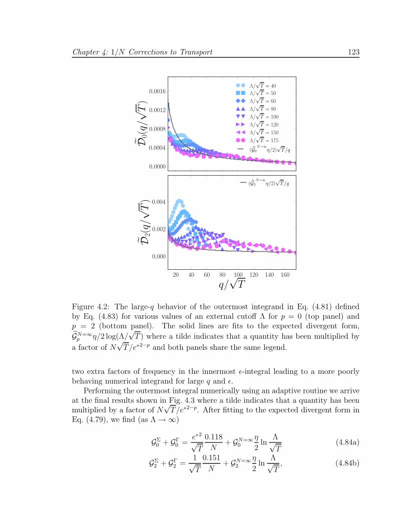
Chapter 4: 1/N Corrections to Transport 123
0.0000
0.0004
0.0008
0.0012
0.0016
D0(
q/√
T)
Λ/√
T = 40
Λ/√
T = 50
Λ/√
T = 60
Λ/√
T = 80
Λ/√
T = 100
Λ/√
T = 120
Λ/√
T = 150
Λ/√
T = 175
(G0N=∞
η/2)√
T/q
20 40 60 80 100 120 140 160
q/√
T
0.000
0.002
0.004
D2(
q/√
T)
(G2N=∞
η/2)√
T/q
Figure 4.2: The large-q behavior of the outermost integrand in Eq. (4.81) definedby Eq. (4.83) for various values of an external cutoff Λ for p = 0 (top panel) andp = 2 (bottom panel). The solid lines are fits to the expected divergent form,GN=∞
p η/2 log(Λ/√
T ) where a tilde indicates that a quantity has been multiplied by
a factor of N√
T/e∗2−p and both panels share the same legend.
two extra factors of frequency in the innermost ε-integral leading to a more poorlybehaving numerical integrand for large q and ε.
Performing the outermost integral numerically using an adaptive routine we arriveat the final results shown in Fig. 4.3 where a tilde indicates that a quantity has beenmultiplied by a factor of N
√T/e∗2−p. After fitting to the expected divergent form in
Eq. (4.79), we find (as Λ→∞)
GΣ0 + GΓ
0 =e∗2
√T
0.118
N+ GN=∞
0
η
2ln
Λ√T
(4.84a)
GΣ2 + GΓ
2 =1√T
0.151
N+ GN=∞
2
η
2ln
Λ√T
, (4.84b)

Chapter 4: 1/N Corrections to Transport 124
0 20 40 60 80 100 120
Λ/√
T
0.00
0.05
0.10
0.15
0.20
0.25
GΣ p+GΓ p
0.118 − 0.13√
T/Λ +(G0
N=∞η/2
)lnΛ/
√T
p = 0
0.151 − 0.54√
T/Λ +(G2
N=∞η/2
)lnΛ/
√T
p = 2
Figure 4.3: The 1/N corrections to thermoelectric transport coming from self-energyand vertex corrections (p = 0 for σ and p = 2 for κ/T ) plotted as a function of adimensionless external ultra violet momentum cutoff Λ/
√T . The solid lines are fits
to the expected divergent behavior, from which one can extract the non-divergentcorrections as Λ→∞.
and combining with the previous results of Eq. (4.69) and (4.71) we have the dcthermoelectric transport coefficients to order 1/N
σ =e∗2
√T
(0.218 +
0.0561
N+
0.0142
Nln
Λ√T
)(4.85a)
κ
T=
1√T
(0.246 +
0.124
N+
0.0161
Nln
Λ√T
), (4.85b)
which both explicitly depend on Λ as expected.
4.3.4 Wiedemann-Franz law in the quantum critical regime
We have evaluated the full fluctuation corrections to thermoelectric transportup to order 1/N (Eqs. (4.85a) and (4.85b)) coming from the direct contributionsof Cooper pairs due to the proximate superconducting state. Initially dismayed bytheir cutoff dependence, we now recall the previous argument that led to Eq. (4.80).We found from scaling that the required T−1/z temperature dependence of κ/T and σ

Chapter 4: 1/N Corrections to Transport 125
0.00 0.05 0.10 0.15 0.20√T/Λ
−0.15
−0.10
−0.05
0.00
0.05
NδW
δW | Λ√T→∞ = 0.038
N
Figure 4.4: The 1/N corrections to the Wiedemann-Franz ratio plotted as a functionof the inverse external rescaled ultra violet momentum cutoff. The solid line is afit to a second order polynomial and the individual divergences of the electrical andthermal conductivity are canceled as Λ/
√T → ∞ giving the universal correction
δW = 0.0376/N .
implied that when dividing them to form the Wiedemann-Franz (WF) ratio, all diver-gent Λ-dependence must exactly cancel. This exact cancellation is seen in Fig. (4.4)where we plot the total correction to the WF ratio, δW as a function of the inverse ofthe rescaled dimensionless cutoff. As Λ→∞, δW approaches a constant. Extractingthe infinite cutoff result via a polynomial fit we find (after inserting the proper powerof the Boltzmann constant)
W =κ
σT=
(0.282 +
0.0376
N
)(kB
e
)2
. (4.86)
Therefore, the WF ratio is indeed obeyed, (i.e. is temperature independent) indicatingthe presence of only fully elastic scattering and is independent of any microscopicconstants. The term proportional to 1/N is quite small, and for the physical case,N = 1 it corresponds to a correction on the order of ten percent.

Chapter 5
Infinite Randomness and ActivatedScaling
The previous three chapters have dealt with the superconductor-metal quantumphase transition as described by a quantum field theory of fluctuating Cooper pairscoupled to an Ohmic bath of fermionic quasiparticles tuned by a pair-breaking in-teraction. Although the role of disorder was briefly discussed in Section 2.7 in termsof a temperature scale above which randomness could be neglected, and estimatesfor model parameters were given in both the clean and dirty limits, the issue hasmostly been ignored. Moreover, the conditions summarized in Table 2.1 hinted at thepossibility that there might be no parametrically large temperature range over whichthe self-interaction between Cooper pairs is large (a requisite condition for universalresults) and weak localization corrections can be neglected. In fact, it was arguedby de Gennes [15] that in the absence of suitably strong bulk or diffusive boundaryscattering, (the clean limit) a superconducting quasi-one dimensional wire in a par-allel magnetic field would be non-ergodic in the sense that time-reversal symmetryis spontaneously broken at long times. The physical implication of non-ergodicityis that the relative phase of the two members of a Cooper pair is not sufficientlyrandomized by the pair-breaking perturbation. The resulting modification of the pairsusceptibility due the interaction which breaks time reversal symmetry cannot cut offthe BCS logarithm, and there will always be a superconducting state down to zerotemperature, where pair fluctuations completely cease.
In this chapter, we vigorously attack the problem of a dirty quasi-one dimensionalsuperconductor at zero temperature in the presence of pair-breaking with great zeal.We will find that not only is disorder a relevant perturbation near the SMT, butthe fixed point is of a quite exotic infinite randomness flavor. The details of thecritical point are investigated using large scale numerical simulations and the rathersurprising conclusion is that the transition is in the same universality class as the onsetof ferromagnetism in the quantum random transverse field Ising model (RTFIM) —a model with discrete symmetry and no dissipation.
126

Chapter 5: Infinite Randomness and Activated Scaling 127
We begin with a brief reminder of the physics of infinite randomness and intro-duce the strong disorder renormalization group with special focus on the recent andsubdolous calculations of Hoyos et al. [129]. We next define a discretized versionof the continuum action studied in Chapters 2 to 4 in the presence of quenched dis-order, and discuss how it can be replaced by an effective quadratic theory in thelarge-N limit. The quadratic theory has a concomitant constraint that is solved via acomputational algorithm we refer to as the solve-join-patch or SJP procedure that ispresented in detail. Finally, we provide both static and dynamic evidence for infiniterandomness and dynamically activated scaling at the SMT through an analysis ofequal time correlation functions, gap statistics and dynamic susceptibilities.
5.1 Strong disorder renormalization group
The role played by quenched randomness in quantum systems is of considerableinterest as disorder correlations are of infinite range in the imaginary time direction.The quantum-classical mapping discussed in Section 1.6 provides little insight here, asdisorder fluctuations can be strongly renormalized by quantum effects and except fora few carefully constructed artificial models, long range disorder correlations rarelyappear in previously studied classical systems. Naively, it might appear that longrange disorder correlations reduce the influence of randomness. However, it turns outthat the opposite is actually true since it is more difficult to integrate out an extendedfluctuation than a local one. As such, the inclusion of randomness in the vicinity ofa quantum phase transition can lead to unusual and non-trivial modifications of theclean critical phenomena [57].
In Chapter 1 the modification of critical behavior in the presence of disorder wasintroduced in the context of the Harris criterion. It was concluded that three outcomeswere possible; disorder is irrelevant and the clean critical behavior is unchanged,disorder is relevant, but there are only quantitative changes to critical exponents,and finally, disorder is relevant and its strength flows to infinity under renormalizationleading to qualitative differences at the critical point and the emergence of non-powerlaw activated scaling. The qualitative change in critical behavior is due to the roleof rare regions, or spurious disorder configurations in the disordered system whichare exponentially rare in their volume. Such regions are manifestly non-perturbativedegrees of freedom and are not accounted for in conventional approximate approaches.As a result, a number of erroneous conclusions were made and it was not until Ma,Dasgupta and Hu [75] applied the strong disorder renormalization group (SDRG)procedure to the random antiferromagnetic spin chain that the physics of rare regionswas fully understood.
The standard momentum shell renormalization group procedure assumes the pres-ence of translational symmetry and is ill suited for disordered systems. The SDRGis essentially an RG in energy space, and since its introduction, it has been success-
Chapter 5: Infinite Randomness and Activated Scaling 128
fully applied to random quantum spin chains [64, 65, 130, 131, 132], ladders [133],random walks [134] and many non-equilibrium systems [135, 136] (for an exhaustivereview see Ref. [137]). The main idea is as follows, at each energy scale, the strongestcoupling in the system is determined, and the ground state of the corresponding partof the Hamiltonian is found exactly. The coupling of this part of the system to theremaining part is treated perturbatively. The excited states of the strongest couplingpiece are neglected and a new effective Hamiltonian is derived with a reduced num-ber of degrees of freedom. This basic step is repeated until some low energy scale isreached.
The SDRG procedure was applied with great success to the RTFIM in one di-mension by D.S. Fisher [64, 65] where he calculated many results exactly and we willintroduce its mechanics in this context here. The transverse field Ising model is oneof the simplest Hamiltonians that is known to undergo a quantum phase transitionas the strength of the transverse field is increased. In the presence of both randomcouplings and fields it is described by the Hamiltonian
H = −∑
i
Jiσzi σ
zi+1 −
∑
i
hi σxi (5.1)
where the σαi are Pauli matrices and the interaction constants Ji and fields hi areindependent random variables drawn from some random distributions. As the modelis one dimensional, a gauge transformation can be performed to make all the Ji andhi positive excluding any possible frustration or the glassy physics that it can incur.
Beginning from this Hamiltonian, the SDRG procedure proceeds as follows. Wefirst determine the maximum coupling in the system defined by Ω = maxi(hi, Ji).Suppose it is the random field at site k, Ω = hk, the part of the Hamiltonian containingthis term is HΩ = −hkσx
k which has ground state | →k〉 and excited state | ←k〉separated by a gap equal to hk. The ground state of σk is mostly unaffected by alongitudinal field (it will make little contribution to the magnetic susceptibility) andit can thus be decimated out of the chain. The coupling of the spin σk to its neighbors,−J1σz
1σz2−J2σz
2σz3 are then treated in second order perturbation theory which results
in a renormalized coupling
J =JkJk+1
hk. (5.2)
The result is a new chain with one less spin and all couplings less than Ω. Onthe other hand, suppose the strongest coupling was a bond, Ω = Jk, then the twospins connected by Jk can flip coherently in a longitudinal field, i.e. the unperturbedpiece of the Hamiltonian −Jkσz
kσzk+1 has two degenerate ground states | ↑k↑k+1〉 and
| ↓k↓k+1〉. These two spins act as an effective composite spin and the fields hk andhk+1 act on it in a perturbative manner described by a renormalized field
h =hkhk+1
Jk(5.3)

Chapter 5: Infinite Randomness and Activated Scaling 129
strong field
h1 h2 h3 h4 h5
J4J1 J = J2J3/h3
strong bond
h1 h2 h3 h4 h5
J4
J1 J2 J3 J4
h = h2h3/J2
J1 J3
J1 J2 J3 J4
Figure 5.1: A schematic representation of a single strong disorder renormalizationgroup step as described in the text for the special case of k = 2. In the presenceof a strong field, a spin is decimated and the adjacent spins are connected by arenormalized bond. If a strong bond is present, two neighboring spins are mergedand experience a renormalized field.
where we have thrown out the antiparallel states and the effective magnetic momentof the new spin cluster is given by
µ = µk + µk+1. (5.4)
Again we have a new spin chain with one less degree of freedom and all couplingssmaller than Ω. In summary, at each RG step, if the strongest coupling is a field, thecorresponding cluster is annihilated and when it is a bond, the two clusters it connectsare joined. This procedure is explained schematically in Fig. 5.1. In the paramagneticphase annihilation dominates as Ω→ 0 and no large clusters are formed, whereas inthe ordered ferromagnetic phase, aggregation dominates as Ω → 0 and at Ω = 0 aninfinite cluster is formed. In this language, the quantum critical point is defined tobe the point where the first infinite cluster appears.
The multiplicative structure of the recursion relations in Eq. (5.2) and (5.3) iscrucial as it leads to the exponential relationship between lengths and energy scales;

Chapter 5: Infinite Randomness and Activated Scaling 130
at each step of the RG, clusters or bonds are added (see Eq. (5.4)) while their couplingsare multiplied. RG flow equations can be written which describe how the probabilitydistributions for ln Ji and lnhi change as the energy is reduced. At the fixed point,these distributions become identical and the solution of the single RG equation leadsto a striking conclusion: lengths and energies are not related in a simple power lawmanner, but scale according to
Lψ ∼ lnΩ0
Ω(5.5)
µ ∼ lnφΩ0
Ω(5.6)
where Ω0 is a reference energy scale. These expressions are starkly different from theusual power law relations between lengths and energies at conventional critical points(Ω ∼ L−z) and the exponential relationship between space and has led to the termactivated dynamical scaling to describe this behavior.
In addition to this novel scaling, Fisher [65] found that at the critical point definedby ln Ji = ln hi (where an overline indicates a disorder average), the probabilitydistributions broaden without limit as the energy scale Ω is reduced. The fact thatthese distributions become infinitely broad is an a posteriori justification of the SDRGprocedure since the recursion relations become asymptotically exactly in this limit.Any fixed point with RG equations that yield infinitely wide probability distributionsfor couplings constants is thus known as an infinite randomness fixed point.
Before discussing the specific critical properties found for the RTFIM, let us makesome general comments on the physics of infinite randomness. In the disorderedphase, there will be some length scale, say ξ, at which the RG procedure describedabove changes qualitatively. For lengths larger than ξ, all fields are larger than allexchange constants and upon further iteration, only fields will be decimated out of thechain leading to longer and weaker bonds, but no new clusters will be formed. Thelength ξ must therefore be related to the physical correlation length which divergeswith the magnitude of the distance from criticality δ as
ξ ∼ δ−ν (5.7)
which defines the correlation length exponent ν. A similar argument can be madein the ordered phase where excitations only exist up to a length scale defined by ξ.At distances longer than ξ, most exchange interactions are larger than any fields andupon further RG iterations all clusters are joined, leading to an infinite cluster forΩ = 0.
The critical exponents ψ, φ and ν from Eqs. (5.5) to (5.7) completely determinethe properties of the infinite randomness fixed point, and for the RTFIM due to theinfinitely wide probability distributions, their values are known exactly to be ν = 2 foraverage correlations (satisfying the Harris criterion dν ≥ 2 in one dimension), ψ = 1/2

Chapter 5: Infinite Randomness and Activated Scaling 131
for tunneling between clusters and φ = (1 +√
5)/2 characterizing the moment of acluster.
Activated scaling is also referred to as highly anisotropic scaling and can lead toextremely slow dynamics in the paramagnetic phase as highly ordered rare regionsfluctuate sedately. This can have important consequences for correlation functionssince their probability distributions will also become very broad with spins located inthe same well-ordered cluster giving contributions to averages of order one. One musttherefore make a distinction between the usual definition of an average observableO(x) and a typical observable Otyp(x) defined by the re-exponentiated average of alogarithm:
O(x) =
∫P (x)O(x) (5.8a)
Otyp(x) = exp
[∫P (x) lnO(x)
](5.8b)
where P (x) is the probability distribution for the random variable x. The distinctionbetween average and typical quantities is a hallmark of infinite randomness criticalpoints and can persist well into the Griffiths region discussed in Section 1.6.
Defining the spin-spin correlation function as
C(x) =⟨σz
i σzi+x
⟩(5.9)
Fisher found that at the critical point (δ = 0)
C(x) ∼1
x2(d−φψ)(5.10a)
Ctyp ∼ e−xψ(5.10b)
whereas in the paramagnetic region where δ > 0
C(x) ∼exp[−(x/ξ)− (27π2/4)1/3(x/ξ)1/3
]
(x/ξ)5/6(5.11a)
Ctyp ∼ e−x/eξ (5.11b)
with ξ defined to be the length scale which describes typical correlations with modifieddivergence
ξ ∼ δ−eν (5.12)
and ν = 1.A natural questions arises regarding how far the SDRG and the results found for
the RTFIM can be generalized to other systems with different symmetries, dimension-ality and interactions. In higher dimensions the aggregation/decimation procedure

Chapter 5: Infinite Randomness and Activated Scaling 132
highlighted in Fig. 5.1 does not lead to analytic recursion relations as the topologyof the lattice is changed with each iteration. Motronich et al. [138] implementeda numerical version of the SDRG for the two dimensional Ising model in a randomtransverse field and find evidence for the flow to strong disorder with modified criticalexponents ν ≈ 1.1, ψ ≈ 0.42 and φ ≈ 2.5. Generalizing the Ising symmetry to a Pottsmodel, Senthil and Majumdar [139] found that any random quantum system with acontinuous quantum phase transition at which a discrete symmetry of a non-conservedorder parameter is broken will have the same critical behavior as the RTFIM; its prop-erties are hyper-universal. Strong disorder physics can even overcome frustration, asat an infinite randomness critical point, the coupling distribution becomes so broadthat in any loop, the frustrated interaction can be neglected. Infinite randomness forIsing symmetry does not survive, however, in the presence of a relaxation mechanismsuch as the coupling to bath degrees of freedom [73, 74]. The tunneling betweenlarge ordered droplets is completely suppressed and the transition is destroyed bysmearing. This behavior can be understood in terms of the localization transition ina dissipative two state system [140].
For disordered O(N) models with continuous symmetry order parameters it ap-pears that in d > 1, any infinite randomness fixed point is unstable and flows to afinite disorder fixed point with conventional power-law scaling. Systems with bothcontinuous symmetry and dissipation — the case studied in this thesis — are onlyjust starting to be understood, and will be the focus of the remaining part of thischapter. Such systems were first studied in the context of itinerant electron systemswhose excitations are damped by coupling between magnetic modes and the gaplessparticle-hole excitations of the metal. Without any damping, the order parameterof a rare region slowly fluctuates and can give rise to quantum Griffiths effects. Asmentioned above, the presence of dissipation retards dynamics, and can lead to thecomplete destruction of the phase transition by smearing [141, 142].
The particular case of d = 1 and Ohmic dissipation z = 2, corresponding to ouroverdamped Cooper pair model with disorder, was recently studied via the SDRGby Hoyos et al. [129]. They found evidence that the SMT is described by a strongdisorder fixed point exhibiting activated dynamic scaling where the logarithm of char-acteristic frequencies of Ψ fluctuations grows as a power of their characteristic lengthscale. They argued further that the strong disorder fixed point is in the same univer-sality class as the one describing the onset of ferromagnetism in the quantum randomtransverse field Ising model in one spatial dimension described in detail above.
Note that this is a non-trivial result, as the RTFIM contains no dissipation, andpossesses a discrete symmetry. The remainder of this chapter presents numericalresults which provide compelling evidence for the applicability of their strong ran-domness RG predictions.
Chapter 5: Infinite Randomness and Activated Scaling 133
5.2 Lattice theory
We begin with a generalized version of the field theory Sα in Eq. (2.1) at zerotemperature which describes the fluctuations of a coarse-grained N -component su-perconducting order parameter Ψa in 1 + 1 dimensions
Sα =
∫dx
∫dτ
[D(x)|∂xΨa(x, τ)|2 + α(x)|Ψa(x, τ)|2 +
u(x)
2|Ψa(x, τ)|4
]
+
∫dω
2π
∫dx γ(x)|ω||Ψa(x,ω)|2.
(5.13)
Quenched disorder has entered the theory through the spatial dependence of all cou-pling constants, D(x), α(x), γ(x) and u(x). We have dropped the tilde on the couplingconstant D as in the dirty limit, it can be identified with the real electron diffusionconstant D = vF3/3. Note that we have not yet performed any rescalings to obtain aunit strength coupling in front of the dissipative |ω| term, allowing for the possibilityof a spatially dependent Ohmic bath.
In our previous studies of this action, we have taken the limit u → ∞ at theoutset to rapidly approach the strong coupling limit, which facilitated the calculationof universal results. In this chapter we will take a slightly different approach, whereu is large with respect to other energy scales, but is still finite, and some results willtake a slightly different form. The loss of translational invariance due to the presenceof disorder inexorably necessitates a numerical approach to fluctuations of the Ψa
field. We first briefly describe the disorder free theory at finite u before introducingthe finite disordered chain that will be our focus for the duration of this chapter.
5.2.1 Infinite clean chain
To ground ourselves, we will first discretize the action on an infinite lattice in theclean limit with a space and time rescaled such that D(x) = 1, α(x) = α, γ(x) = γ = 1and u(x) = u
S =∞∑
j=1
∫dτ[|Ψa,j(τ)−Ψa,j+1(τ)|2 + α|Ψa,j(τ)|2 +
u
2|Ψa,j(τ)|4
]
+
∫dω
2π
∞∑
j=1
|ω||Ψa,j(ω)|2(5.14)
where Ψa,j(τ) is the ath component of the order parameter at lattice site j and imag-inary time τ and
Ψa,j(ω) =
∫dτΨa,j(τ)e
iωτ (5.15)

Chapter 5: Infinite Randomness and Activated Scaling 134
is the Fourier transform of Ψa,j(τ). In the large-N limit, the methods introduced inChapter 3 can be straightforwardly generalized to the finite u case in order to derivethe effective quadratic action (now suppressing the a subscript on all fields)
S0,c =∑
j
∫dτ[D|Ψj(τ)−Ψj+1(τ)|2 + r|Ψj(τ)|2
]+
∫dω
2π
∑
j
|ω||Ψj(ω)|2. (5.16)
The renormalized distance from criticality, r must be found from the self-consistency(saddle point) condition
r = α + u⟨|Ψj(τ)|2
⟩S0,c
= α + u
π∫
−π
dk
2π
Λω∫
0
dω
π
1
r + ω + 2(1− cos k), (5.17)
and as usual, we have absorbed a factor of N into a redefinition of the quartic coupling,introduced a large frequency cutoff Λω and set the lattice constant to unity. Thequantum critical point is found by choosing α = αc so that r = 0 and hence takingthe cutoff Λω = π2 we find
αc = −u
π∫
−π
dk
2π
π2∫
0
dω
π
1
ω + 2(1− cos k)(5.18)
= −2u
πasinh
(π2
)(5.19)
and for u = 1, αc + −0.785. It will be useful to keep the clean value of αc in mindwhen we discuss the disordered theory as it provides an upper bound.
5.2.2 Finite disordered chain
Motivated by the calculations of Hoyos et al. [129] we desire to confirm theirproposition that in the presence of Ohmic dissipation, quantum fluctuations stronglyrenormalize the effects of disorder, leading to a quantum phase transition between asuperconductor and metal governed by an infinite randomness fixed point with theassociated dynamically activated scaling.
As mentioned above, quenched disorder can be introduced into a L-site latticediscretization of the our continuum overdamped Cooper pair model Sα at T = 0
S =
∫dτ
L−1∑
j=1
Dj |Ψj(τ)−Ψj+1(τ)|2 +L∑
j=1
[αj|Ψj(τ)|2 +
uj
2|Ψj(τ)|4
]
+ cl|Ψ1(τ)|2 + cr|ΨL(τ)|2
+
∫dω
2π
L∑
j=1
γj|ω||Ψj(ω)|2, (5.20)

Chapter 5: Infinite Randomness and Activated Scaling 135
where all couplings are random functions of j and we have introduced fixed butrandom boundary conditions cl and cr, similar to those employed in Ref. [89] todescribe the effects of leads on the conductance of ultra-narrow finite length metallicwires. The quartic coefficients uj must all be positive to ensure stability and repulsionbetween Cooper pairs. The dissipation into the metallic bath as represented by γj,is also required to be positive by causality. Finally, we can choose a gauge such thatDj > 0. A more careful analysis and suitable rescalings [110] allow us to reduce therandomness to only the spatial dependence of Dj and αj while setting uj = u andγj = 1. Disorder in these two couplings alone is sufficient to generate disorder in γj
under renormalization.The random diffusion constant Dj is taken to be uniformly distributed on (0, 1]
P (Dj) =
1 ; 0 < Dj ≤ 10 ; otherwise
(5.21)
such that its mean D = 1/2 while αj is assumed to be Gaussian distributed with
mean α and standard deviation√α2 − α2 = 1/2 in units of γ2
P (αj) =
√2
πe−2(αj−α)2 . (5.22)
At zero temperature, the SMT can be tuned by reducing the mean of the αj distri-bution, α, while keeping its variance constant.
Equivalently, we could have also chosen to work in a lattice model of fluctuatingphases with Ψj(τ) = eiθj(τ) of unit magnitude [89, 93]; this should have the sameproperties as S, but our analysis proceeds more conveniently by also allowing formagnitude fluctuations.
While S is a suitable model for describing the influence of disorder on the fluctuat-ing Cooper pair states, we also have to consider the effect of randomness on the singleelectron states. We have estimated such effects in the framework of weak-couplingBCS theory: at criticality, we find that on a scale parametrically smaller than thesingle electron localization length, the gain in condensation energy can offset the costin elastic energy when order parameter fluctuations take advantage of randomnessin the αj . This justifies our focus on the influence of disorder in a purely bosonicoverdamped Cooper pair theory (see Ref. [43]).
The RG analysis [129] was carried out in a model with an N -component orderparameter and it was found that flows had only an irrelevant dependence on the valueof N [143]. Thus the exact critical properties can be obtained by studying the modelin the large-N limit. As above, this is equivalent to approximating S by the Gaussian
Chapter 5: Infinite Randomness and Activated Scaling 136
action
S0 =
∫dω
2π
[L−1∑
j=1
Dj |Ψj(ω)−Ψj+1(ω)|2 +L∑
j=1
(rj + |ω|)|Ψj(ω)|2
+ cl|Ψ1(ω)|2 + cr|ΨL(ω)|2]
=L∑
j=1
∫dω
2πΨ∗
j (ω) (Mij + |ω|δij)Ψj(ω) (5.23)
where the frequency independent coupling matrix is given by
Mij =
D1 + cl + r1 ; i = j = 1DL−1 + cr + rL ; i = j = L(Di + Di−1 + ri)δi,j −Djδi,j+1 −Diδi,j−1 ; otherwise
(5.24)
with each rj determined self-consistently by solving the now site dependent saddlepoint equation
rj = αj +⟨|Ψj(τ)|2
⟩S0
, (5.25)
and we have set u = 1 to reach a strong coupling regime. In this simplified form, theaverage equal time on-site order parameter susceptibility in Eq. (5.25) is given by
⟨|Ψj(τ)|2
⟩S0
=
∫dω
2π[ |ω|1 + M ]−1
jj (5.26)
where 1 is the L× L identity matrix.From Eq. (5.24), it is clear that M is a real, symmetric tridiagonal matrix (due
to the fixed boundary conditions chosen), and it will convenient to find its spectraldecomposition in terms of the eigenvector Vij and accompanying diagonal eigenvalueEij = λjδij matrices defined by
L∑
j=1
MijVjk = Vikλk (5.27)
where V is orthogonal. This decomposition can be used to write inverses involving M
like the one in Eq. (5.26) as
[ |ω|1 + M ]−1ij =
L∑
k=1
VikVkj
|ω| + λk(5.28)
and thus the saddle point equation is given by
Qi ≡1
π
L∑
j=1
(Vij)2 ln
(1 +
π2
λj
)+ αj − rj = 0 (5.29)

Chapter 5: Infinite Randomness and Activated Scaling 137
where we sum over the ith component of each eigenvector and have introduced an ultraviolet cutoff Λω = π2 for convergence of the frequency integral. It will be convenientto introduce the analytical form of the Hessian matrix at the saddle point given by
∂Qi
∂rj= −δi,j −
u
π
L∑
k,/=1
VikVjkVi/Vj/lnλk − lnλ/λk − λ/
. (5.30)
By the use of the spectral decomposition of M we have eliminated the need to computeits inverse and are left with the task of diagonalizing a tri-diagonal matrix which canbe accomplished using a standard QL algorithm which scales linearly with the numberof sites L.
5.3 The solve-join-patch algorithm
Solving the innocuous looking Eq. (5.29) for a large number of disorder realizationsand large system sizes was the primary time-consuming numerical step in obtainingthe results of this chapter. Similar numerical large-N methods have been used previ-ously for disordered systems with conventional (power law) dynamic scaling [144, 145]but the presence of activated scaling leads to sluggish dynamics and the necessity toproperly include spurious disorder configurations that, although exponentially rare,can make large contributions to thermodynamic properties. The full numerical so-lution corresponding to the set rj for a given realization of disorder, system sizeL and mean random pair-breaking α can be obtained by an iterative process usinga modified version of Powell’s hybrid method [146, 147]. The computational effortis drastically reduced by having access to the analytic form of the Hessian matrixgiven in Eq. (5.30). This approach works quite well for large α or small system sizes,but as we draw nearer the critical point, characterized by the crossover conditionthat the correlation length ξ ∼ L, the direct iterative solution of Eq. (5.25) quicklybecomes computationally prohibitive. This is a result of the fact that the eigenmodesof S0 begin to delocalize and have a characteristic energy scale that is exponentiallysmall in the distance from criticality, requiring that the solutions rj be computedwith exponentially increasing precision.
This obstacle was overcome through the development and implementation of aniterative solve-join-patch (SJP) procedure in the spirit of real space renormalization.It takes advantage of the presence of only short range nearest neighbor interactionsin the effective action Eq. (5.23). The SJP algorithm which can be applied to verylarge systems near criticality is shown schematically in Fig. 5.2. Algorithmically, itis defined by the following steps.
1. Generate a realization of disorder for a system composed of L = n3 sites, labeledby i = j3+ k where 0 ≤ j ≤ n− 1, 1 ≤ k ≤ 3 and n is an even integer.

Chapter 5: Infinite Randomness and Activated Scaling 138
joinjoin
patch
solve
solve
L = 64
solve solve solve
patch
solve
Figure 5.2: A schematic outline of one iteration of the solve-join-patch procedure forthe specific case of L = 64 with n = 4 and 3 = 16.
2. Break the large system into n subsystems of size 3 and iteratively solve Eq. (5.29)for each subsystem via Powell’s method described above, with the modificationthat for interior systems (0 < j < n− 1), the fixed boundary conditions previ-ously Determined by the random numbers cl and cr are replaced by cl = Jj/ andcr = Jj/+/+1. The result is n sets of 3 ri’s which solve the individual subsystemself-consistency equations, (5.29).
3. Join the now solved n subsystems into n/2 larger subsystems of length 23. Notsurprisingly, Eq. (5.29) for the new enlarged subsystem will be poorly satisfiednear the interfaces where the neighboring values of ri are poorly matched. Thiscan be addressed through a patching procedure where one considers a smallmini-system composed of only six sites, centered at the joint.
4. For each subsystem whose left half is labeled by j construct the mini-systemcomposed of the sites i = j3 + 3 − 2, . . . , j3 + 3 + 3. Set cl = Jj/+/−3 andcr = Jj/+/+4 and iteratively solve for the six new values r′i. With thesenew values included, each subsystem of length 23 is now quite close to sat-isfying Qi = 0 and can be quickly solved using the set of initial conditionsrj/+1, . . . , rj/+/−3, r′j/+/−2, . . . , r
′j/+/+3, rj/+/+4, . . . , rj/+2/ producing a solution
set ri.

Chapter 5: Infinite Randomness and Activated Scaling 139
5. Redefine 3→ 23, n→ n/2.
6. Iteratively repeat the SJP procedure outlined in steps 3 → 5 until a self-consistent solution is found to Qi = 0 for the full system composed of L sites(n = 1, 3 = L).
Although the SJP method works quite well, we are still limited by the requirementof performing a full diagonalization of larger and larger matrices and have consideredup to 3000 realizations of disorder for the four system sizes, L = 16, 32, 64, 128. Thethermodynamic limit is approximated by finite size scaling where appropriate.
5.4 Evidence for infinite randomness
Fisher’s remarkable solution of the RTFIM [64, 65] includes asymptotically exactresults for the exponents and correlation functions at the infinite randomness fixedpoint, and many directly translate to the RG calculations by Hoyos et al. [129] forthe dissipative model considered here. In particular, one expects activated dynamicscaling with ln(1/Ω) ∼ Lψ where Ω is a characteristic energy scale and ψ = 1/2is a tunneling exponent. This reflects the fact that at an infinite randomness fixedpoint, the dynamical critical exponent z is formally infinite. The RG approach definesa real space decimation procedure that either creates or destroys clusters or bondsas the energy scale is reduced. The typical moment of a surviving cluster scales likeµ ∼ lnφ(1/Ω) at criticality, where φ = (1+
√5)/2 + 1.62 is the golden mean. Average
correlations are described by a correlation length which diverges as ξ ∼ |δ|−ν withν = 2 and δ a measure of the distance from criticality. From Ref. [129], δ is expectedto be proportional to ln(ri/rc) where rc is some critical value. Our numerical studyreveals that close to criticality this quantity is linearly related to the detuning of theaverage α from its quantum critical value, αc, (which has yet to be determined) andit further demonstrates that correlations among the ri due to their self-consistencydoes not affect the strong randomness RG flow.
The remainder of this chapter will present a numerical confirmation of the resultsof Ref. [129] by providing arguments for the presence of dynamically activated scalingat the quantum SMT, characterized by exponents ν, ψ and φ taking on their RTFIMvalues. The evidence comes from an analysis of equal time correlations, energy gapstatistics and dynamic susceptibilities in the weakly disordered quantum Griffithsphase [70].
5.4.1 Equal time correlation functions
We begin by studying the disorder averaged equal-time correlation function
C(x) = 〈Ψ∗x(τ)Ψ0(τ)〉S0
, (5.31)

Chapter 5: Infinite Randomness and Activated Scaling 140
5 10 15 20 25 30x
10−8
10−7
10−6
10−5
10−4
10−3
10−2
10−1
100
101
102
C(x
)
αc = −0.93(3)ν = 1.9(2)
α0.00-0.25-0.50-0.65-0.75
−2.0 −1.5 −1.0 −0.5 0.0
ln δ
0
1
2
3
lnξ
Figure 5.3: The equal-time disorder averaged correlation functions for L = 64 and fivevalues of the mean of the αj distribution, α. The solid lines are fits to the asymptoticform described in Eq. (5.32) via ξ and an overall scale parameter. The inset showsthe result of a fit to the power law form of the finite size scaled correlation lengthleading to an estimate for the location of the critical point αc = −0.93(3) and thecorrelation length exponent ν = 1.9(2).
(where x is now a site index) which can be computed from the quadratic effective ac-tion S0 once the full set of solutions rj has been obtained, and an overline indicatesan average over realizations of disorder. In the disordered phase, where δ ≡ α−αc > 0the asymptotic form of C(x) for the RTFIM has been predicted to describe both ex-ponential as well as stretched exponential decay in addition to power law behavior[65]
C(x) ∼exp[−(x/ξ)− (27π2/4)1/3(x/ξ)1/3
]
(x/ξ)5/6. (5.32)
If we use this expression to define the correlation length ξ, we can perform fits foreach value of L and various α to extract ξ(L,α) as is seen in Fig. 5.3 for L = 64. Wefind remarkable agreement (solid lines) with Eq. (5.32) over six orders of magnitudefor all system sizes considered.
As mentioned above, the length scale which describes average correlations is ex-pected to diverge like ξ ∼ |δ|−ν as the critical point is approached. We have employedthis result to perform a log-log fit to the finite size scaled correlation length (dataextrapolated to L →∞) as a function of δ, as is shown in the inset of Fig. 5.3. The

Chapter 5: Infinite Randomness and Activated Scaling 141
0 5 10 15 20 25 30
|α− αc|νL
0.0
0.2
0.4
0.6
0.8
1.0
1.2
ξ/L
L128643216
Figure 5.4: Data collapse of the finite size data for the correlation length using αc =−0.93 and ν = 1.9 highlighting the consistency of the finite size scaling and fittingprocedures.
value of αc was found from the mean of the critical αj distribution which minimizedthe least square error of power law fits involving δ = α− αc. This leads to a value ofαc = −0.93(3) for the critical point and ν = 1.9(2) for the correlation length expo-nent with the number in brackets indicating the uncertainty in the last digit computedfrom the fitting procedure. The obtained value of ν is in accord with the value of 2predicted for the RTFIM. The correlation length could also have been defined via theexponential tail of C(x) at large separations which yields compatible values for bothαc and ν. The accuracy of the finite size scaling and fitting results was confirmedthrough the observation of good data collapse when plotting ξ(L, δ)L−1 against δν L[52] as seen in Fig. 5.4.
5.4.2 Energy gap statistics
For each realization of disorder and each value of α we define the gap Ω(L) tobe the smallest excitation energy in the system, which in general corresponds to themost delocalized mode of S0. Rare disorder configurations cause clusters to behaveas if they were much more critical than the global value of δ would suggest. Theseclusters dominate the critical modes and exhibit abnormally small gaps that make

Chapter 5: Infinite Randomness and Activated Scaling 142
−25 −20 −15 −10 −5 0
lnΩ10−4
10−3
10−2
10−1P
(lnΩ
)
δ = 0.18
L128643216
−8 −6 −4 −2 0
lnΩ
δ = 0.93
Figure 5.5: The system size dependent probability distribution (over all realizations ofdisorder) for the logarithm of the gap (minimum eigenvalue) for α close to criticality(left panel) and far from criticality (right panel) where δ = α− αc with αc = −0.93.
large contributions to disorder averages of lnΩ, leading to the highly anisotropicscaling relationship between space and time that is the hallmark of strong disorderfixed points. We have performed a direct analysis of the probability distribution forthe logarithm of the energy gap with the result shown in Fig. 5.5. We observe thatwhen the mean of the αj distribution is close to its critical value (left panel) the gapdistribution gets broader with increasing system size, characteristic of having more“space” in the sample where a strongly ordered (rare) region can form. Far fromcriticality (right panel) the histograms look very similar for different system sizesand are just horizontally shifted from one another. This is consistent with the ideathat well into the disordered phase the excitations leading to a small gap are welllocalized and have a probability proportional to L. The drastic change in qualitativebehavior between δ = 0.18 and δ = 0.93, with the width of the small δ distributionstrongly depending on system size, provides cogent evidence for z = ∞ at the criticalpoint. A similar analysis for the RTFIM was carried out by Young and Rieger [148]where they found identical results. In addition we find that lnΩ, as the minimalexcitation energy, is naturally characterized by extreme value statistics and has aGumbel probability distribution
P (x) =1
βexp
[(x− µ
β
)− exp
(x− µ
β
)](5.33)

Chapter 5: Infinite Randomness and Activated Scaling 143
−20 −15 −10 −5
lnΩ10−3
10−2
10−1
P(l
nΩ
)
L = 128
δ = 0.18Gumbel
Figure 5.6: A fit of the probability distribution of the minimum excitation energy forsystem size L = 128 and δ = 0.18 (symbols) to a Gumbel distribution with locationµ + −9.2 and scale β + 2.3 (solid line). The Gumbel form is not unexpected as thelogarithm of the gap for each realization of disorder is an extremal value.
with location µ and scale β. A Gumbel fit for L = 128 and δ = 0.18 is shown inFig. 5.6.
If activated dynamic scaling is indeed present, the disorder averaged value of thelogarithm of the gap should scale like
|lnΩ| ∼ ξψ ∼ δ−νψ (5.34)
where we have used the scaling form of the correlation length. Such divergent behaviorfor the finite size scaled value of |lnΩ| is demonstrated in Fig. 5.7. The possibility ofconventional scaling was considered but ultimately excluded through the examinationof the maximum likelihood estimator for a wide range of power law fits. Using thepreviously determined values of αc and ν, the tunneling exponent can be extractedfrom a log-log linear fit of the average logarithmic spectrum as shown in the inset ofFig. 5.7, producing ψ = 0.53(6) which is consistent with the RTFIM prediction of 1/2.A final consistency check is to investigate data collapse for the probability distributionof the rescaled logarithmic energy scale δνψ lnΩ near criticality as detailed in Fig. 5.8.

Chapter 5: Infinite Randomness and Activated Scaling 144
0.5 1.0 1.5 2.0 2.5
δ0
2
4
6
8
10
12
14
16
|lnΩ|
ψ = 0.53(6)
−2.0 −1.5 −1.0 −0.5 0.0
ln δ
0.0
0.5
1.0
1.5
2.0
2.5
3.0
ln|ln
Ω|
Figure 5.7: The finite size scaled value of the disorder averaged logarithm of theminimum excitation energy plotted against the distance from the critical point δ. Weobserve divergence consistent with the scaling form |lnΩ| ∼ δ−νψ and using the valueof αc and ν found above we determine ψ = 0.53(6) from a log-log linear fit (inset).
5.4.3 Dynamical Susceptibility
To confirm full agreement with the universality class of the RTFIM, we mustfinally determine the value of the exponent φ which controls the average moment,µ ∼ | lnω|φ, of a cluster fluctuating with frequency ω. This can be accomplished byinvestigating the imaginary part of the disorder averaged dynamical order parametersusceptibilities after they have been analytically continued to real frequencies. Weare interested in the average (k = 0) and local susceptibilities defined by
Im χ(ω) =1
L
∑
x
Im 〈Ψ∗x(iω)Ψ0(iω)〉S0
∣∣∣iω→ω+iε
(5.35a)
Im χloc(ω) = Im 〈Ψ∗0(iω)Ψ0(iω)〉S0
∣∣∣iω→ω+iε
(5.35b)
respectively, where 〈· · · 〉S0 indicates an average with respect to the large-N action inEq. (5.23) and x = |i− j| is the separation between two sites. Note that ω is now areal frequency, and we point out that our facile access to such dynamical quantitiesis one of the perquisites of the numerical approach we have taken. All frequencies aremeasured with respect to an ultra-violet cutoff Λω which is required for convergencewhen computing the set of solutions to Eq. (5.25).

Chapter 5: Infinite Randomness and Activated Scaling 145
−6 −5 −4 −3 −2 −1
δνψ lnΩ
10−4
10−3
10−2
10−1
P(δ
νψ
lnΩ
)
δ
L = 128
0.430.280.18
Figure 5.8: The rescaled probability distribution for the natural logarithm of thesmallest excitation energy for L = 128 and δ = 0.18, 0.23, 0.43 which exhibits datacollapse consistent with activated scaling for the values αc = −0.93, ν = 1.9 andψ = 0.53 discussed in the text.
The spectral decomposition of the coupling matrix M introduced in Section 5.2.2can be used here to derive explicit results for the average and local susceptibility,whose forms will be useful in determining scaling relations. For a single realizationof disorder, Eq. (5.28) leads to an expression for the dynamic order parameter sus-ceptibility between two sites i and j at imaginary frequency iω
χij(iω) = 〈Ψ∗i (iω)Ψj(iω)〉S0
= [ |ω|1+ M ]−1ij
=L∑
k=1
VikVkj
|ω| + λk(5.36)
where λk is an eigenvalue corresponding to the kth column of the eigenvector matrixV. The local susceptibility is an average over all sites of the response to a local “field”

Chapter 5: Infinite Randomness and Activated Scaling 146
at each site
χloc(iω) =1
L
L∑
i=1
χii(iω)
=1
L
L∑
i,j=1
(Vij)2
|ω| + λj
=1
L
L∑
i=1
1
|ω| + λi(5.37)
where we have used the orthogonality of V. Analytically continuing to real frequenciesiω → ω + iη and taking the imaginary part of both sides
Imχloc(ω) =1
L
L∑
i=1
ω
ω2 + λ2i
(5.38)
where we immediately observe that Imχloc ∼ ω−1 for ω . Ω and Imχloc ∼ ω forω * Ω, with the gap Ω = miniλi.
Identical arguments lead to an expression for the average susceptibility defined asthe k = 0 component of the spatial Fourier transform of χij(iω)
Imχ(ω) =1
L2
L∑
i,j,k=1
ωVikVjk
ω2 + λ2j
(5.39)
which should have the same leading frequency dependence as Imχloc except the ex-pressions will be modified by a term
∑ij VikVjk which is directly related to the mag-
nitude of local order (the cluster moment).Appendix D provides a detailed derivation of the scaling forms for the dynamical
susceptibilities in the quantum Griffiths region, and from Eq. (D.16a) and Eq. (D.16b)
Imχloc(ω) ∼δ1/ψ−φνδ
(δνψ | lnω |
)δ/ψ
ω1−δ/ψ. (5.40)
Imχ(ω) ∼δ1/ψ−φνψ(1+δ/ψ)
(δνψ | lnω |
)1−δ/ψ
ω1−δ/ψ. (5.41)
The disorder averaged dynamical susceptibilities are plotted for δ > 0 in Figs. 5.9and 5.10 for L = 128 with insets that show data collapse confirming the predictedscaling behavior of Eqs. (5.40) and (5.41). The leading order frequency dependenceof both susceptibilities can be understood as follows: for ω " Λω = π2 we find atrivial 1/ω behavior, independent of δ. However, as argued above, the non-trivialfrequency dependence of the susceptibility can be understood in terms of the relative

Chapter 5: Infinite Randomness and Activated Scaling 147
10−510−410−310−210−1 100 101 102 103 104 105
ω10−3
10−2
10−1
100
101
102
103
104
105
χlo
c
δ0.930.680.430.280.18
0 2 4 6 8 10
δνψ| ln ω|100
101
102
103
ωλ
1δλ
3χ
loc
Figure 5.9: The disorder averaged local dynamical susceptibility for five values of δ inthe quantum Griffiths phase with L = 128. The inset shows data collapse compatiblewith Eq. (5.40) where λ1 = 1− δ/ψ and λ3 = φνδ − 1/ψ.
size of ω when compared to the energy of the most critical mode, labeled by Ω. Forω * Λω and δ ∼ 1 we are far from criticality and all modes are well localized. Theprobe frequency is the smallest energy scale in the system and the susceptibility islinear in ω. When δ * 1, vanishingly low energy modes may appear as a consequenceof strongly ordered rare regions; the susceptibility is now inversely proportional toprobe frequency.
Physically, one can argue that the average cluster moment will be given by theratio of the average to local susceptibility due to the extra sum over sites implicit inin Eq. (5.35a). This is proven in Appendix D, and we define
R(ω) =Imχ(ω)
Imχloc(ω)∼ | lnω|φ ΦR
(δνψ| lnω|
), (5.42)
where the scaling function ΦR approaches a constant when the dimensionless variableδνψ| lnω|* 1. In the quantum disordered phase with δνψ| lnω|. 1, a scaling analysis(Appendix D) predicts ΦR(x) ∼ x1−φ and hence
R ∼ δνψ(1−φ)| lnω|. (5.43)
In order to determine the value of φ, it is useful to consider a rescaled value of thesusceptibility ratio
R(δ) =R(ω)
δνψ| lnω|(5.44)

Chapter 5: Infinite Randomness and Activated Scaling 148
10−510−410−310−210−1 100 101 102 103 104 105
ω10−5
10−4
10−3
10−2
10−1
100
101
102
103
104
χ
δ0.930.680.430.280.18
0 2 4 6 8 10
δνψ| ln ω|0.0
0.5
1.0
1.5
2.0
2.5
ωλ
1δλ
2χ
Figure 5.10: The disorder averaged average dynamical susceptibility for five valuesof δ in the quantum Griffiths phase with L = 128. The inset shows data collapsecompatible with Eq. (5.41) where λ1 = 1− δ/ψ and λ2 = φνψ(1 + δ/ψ)− 1/ψ.
which should be frequency independent according to the predicted scaling form forR(ω) as ω → 0. We plot the finite size scaled susceptibility ratio in Fig. 5.11 forthe three smallest values of δ, and find confirmation of its linear | lnω| dependence.The inset of Fig. 5.11 confirms the frequency independence of R and by determiningthe best linear fit of ln R to ln δ for ω ≤ 10−3 with νψ = 1.0(1), we find a clusterexponent φ = 1.6(2) which is very close to the predicted RTFIM value of (1 +
√5)/2.
5.4.4 Summary
The results of the previous section, as highlighted in Figs. 5.3, 5.7 and 5.11, providecompelling evidence for the applicability of the real space RG analysis of Hoyos etal., and further reproduces a number of results of [65] to unexpected accuracy. Thisconfirms that the considered model for overdamped repulsive Cooperon fluctuations inthe presence of quenched disorder near a SMT exhibits dynamically activated scalingand is controlled by an infinite randomness fixed point in the same universality classas the RTFIM with the schematic phase diagram shown in Fig. 5.12. As summarizedin Table 5.1, the transition is characterized by the numerically computed criticalexponents (ν,ψ,φ) + (1.9, 0.53, 1.6) which are entirely consistent with those of theone dimensional random quantum Ising model in a transverse field (2, 1/2, (1+
√5)/2).

Chapter 5: Infinite Randomness and Activated Scaling 149
6 8 10 12 14
| ln ω|0.00
0.02
0.04
0.06
0.08
0.10
0.12
0.14
R
φ = 1.6(2)
δ0.430.280.18
−2.0 −1.5 −1.0 −0.5
ln δ
−6
−5
−4
−3
lnR
| lnω|16.114.513.812.2
Figure 5.11: The real frequency dependence of the finite size scaled value of thedisorder averaged susceptibility ratio defined in Eq. (5.42) for three values of δ =α−αc. We observe the predicted | lnω| behavior. After a suitable rescaling describedin the text we find that R does not depend on frequency as ω → 0 (inset), and alog-log linear fit gives the value of the cluster exponent to be φ = 1.6(2).
ν ψ φ
RTFIM 2 1/2 (1 +√
5)/2
Ohmic Cooperon Theory 1.9(2) 0.53(6) 1.6(2)
Table 5.1: A summary and comparison of the critical exponents describing the correla-tion length (ν), tunneling (ψ) and cluster moment (φ) for the onset of ferromagnetismin the quantum random transverse field Ising model (RTFIM) where their values areasymptotically exact, and the zero temperature quantum phase transition between asuperconductor and a metal in a dissipative theory of Cooperon fluctuations coupledto an Ohmic bath which have been calculated numerically.

Chapter 5: Infinite Randomness and Activated Scaling 150
QC
SC N
T
δIRFPFigure 5.12: A schematic phase diagram for the transition between a superconduct-ing (SC) and normal (N) state connected by an infinite randomness fixed point(IRFP). The shape of the finite temperature phase boundary was predicted to beTc ∼ exp(−C|δ|νψ) in Ref. [129] where C is a constant.

Chapter 6
Conclusions
This thesis has been concerned with a topic that could be mistakingly confusedwith one of limited scope, the pair-breaking quantum phase transition between asuperconductor and a metal in an ultra-narrow wire as modeled by a continuumquantum field theory. Instead, we have discovered a remarkably rich phase diagramfull of interesting phases and crossovers, and even the presence of infinite randomnessand exotic non-power law activated scaling relations between space and time in thepresence of disorder.
Experimental motivations exist in the form of transport experiments on metallicnanowires, formed through molecular templating by sputtering material on top of along rigid “bridge” or “backbone” molecule lying over a trench [35]. In this way, wireswith diameters of less than 10 nm can be fabricated; a giant step towards reachingthe quantum limit. In an applied current and at fixed temperatures, below the bulksuperconducting transition temperature for the wires composite material, a givenwire can display either metallic or superconducting behavior depending on its radius,with the general trend that thinner wires are less superconducting. In addition, for aparticular wire which does exhibit electrical transport without resistance, supercon-ductivity can be destroyed by turning on a suitably strong magnetic field orientedalong its parallel axis. In both of these cases, it is some non-thermal parameter whichtunes between the superconducting and normal metallic state at zero temperatureproviding an excellent manifestation of a quantum phase transition.
The description of the transition that we have adopted in this thesis is in terms ofa critical theory of strongly repulsive, fluctuating Cooper pairs, written in terms of acomplex order parameter overdamped by its coupling to a bath of unpaired fermionsresulting from the presence of some type of pair-breaking interaction. The existence ofthe bath, imagined as a large number of unpaired electrons residing in the transverseconduction channels of the wire, leads to a long range interaction in imaginary timeproviding Ohmic dissipation in the form of a non-analytic |ωn| term in the effectiveaction. The presence of such an anisotropic relationship between space and time inthe presence of a continuous symmetry order parameter fixes the dynamical critical
151

Chapter 6: Conclusions 152
exponent at z = 2, and the resulting upper critical dimension is dUCD = 2.The thinness of these wires provided us with a useful theoretical framework in the
form of the quasi-one dimensional limit, where the radius of the wire R is on the orderof, or much smaller than the superconducting coherence length ξ0 at low temperatures.The length scale ξ0 measures the average separation between the electrons in a Cooperpair, and as R < ξ0 they begin to feel the boundary. If the wire is sufficiently long,the paired states can be described in terms of a quantum field theory in one space andone imaginary time dimension. In 1 + 1 dimensions, we found ourselves below dUCD,with the repulsive self-interactions between Cooper pairs being strongly relevant. Asa result, any perturbative or mean field approaches were unable to provide a completeand accurate picture of the physical phenomena.
By employing a large number of field theoretic and numerical techniques in con-junction with a careful scaling analysis, we have determined the behavior of the zerofrequency (dc) conductivity as a function of temperature and the pair-breaking pa-rameter which drives the transition. Our first experimentally testable result is acomplete crossover phase diagram for the quantum superconductor-metal transition(SMT). We predict that upon fixing the source of pair-breaking (either magnetic fieldor wire radius) at a value near criticality, as function of decreasing temperature, theconductivity should first increase as 1/
√T due to the influence of the quantum crit-
ical point, then change to decreasing as T 2 once the low temperature metallic phasehas been reached. There is already qualitative evidence for transport in this regimethat is non-monotonic in temperature.
The second prediction is that in the quantum critical regime at finite tempera-tures, defined by a pair-breaking strength that is close to the one that would destroyorder at zero temperatures, the ratio of dc thermal (κ) to electrical (σ) conductivity(the Wiedemann-Franz ratio) should be linear in temperature, with a proportionalityconstant that is corrected from the Lorenz number for a normal metal. We havecomputed the exact value of this correction in a systematic expansion in the inversenumber of complex order parameter components N and found
W ≡κ
σT=
(0.282 +
0.0376
N
)(kB
e
)2
. (6.1)
Conversations with experimentalists have been initiated on the feasibility of per-forming thermal transport experiments on nanowires and we are hopeful that suchmeasurements will be made in the foreseeable future.
Further avenues for theoretical progress still remain in these systems, includinga full understanding of the low temperature ordered phase which has not been at-tempted here. Such a description would require proper inclusion of the pairing in-teraction as well as Coulomb repulsion, leading to a plasmon mode describing thestrongly fluctuating phase of the superconducting order parameter.
Possible real time approaches like Keldysh or even the density matrix renormal-ization group (DMRG) might also offer directions of attack. In particular, it would

Chapter 6: Conclusions 153
be of considerable interest to determine the best method for simulating an Ohmicbath in DMRG by approximating the formally infinite number of degrees of freedomthat would exist at each spatial location.
The role of randomness in the nanowire transport experiments is still an openquestion, as it can be difficult to obtain an accurate picture of how much disorderis present in the real ultra-narrow wires beyond estimates inferred from their normalstate resistance. There is some evidence that the surface of the wires may be hometo localized magnetic impurities but beyond that little is known. The theoreticalinclusion of disorder is straightforward in principle, and can be done by allowing anycoupling constants to have an explicit spatial dependence.
Spurred on by some compelling strong disorder RG results, we have simulated alarge number of finite length disordered wires ranging from 16 to 128 “sites”. At zerotemperature, we analyzed both equal time and dynamic correlation functions andfound a phase transition between a superconductor and metal described by an infi-nite randomness fixed point. The physics near such a critical point has some unusualand fascinating properties due to the contribution of rare regions, including highlyanisotropic scaling relations between space and time (activated scaling) and a mea-surable difference between the average and typical values of macroscopic observables.An even more interesting property of this transition is that it is fully described bythree critical exponents, ν + 1.9 which determines the diverging length scale describ-ing average equal time order parameter correlations, ψ + 0.53 a tunneling exponentwhich relates the logarithm of the characteristic frequency of fluctuations to theirwavevector and φ + 1.6 which fixes how the magnitude of a critical mode describinglocal order scales with the logarithm of its characteristic frequency. These exponentsare in full agreement with ν = 2, ψ = 1/2 and φ = (1 +
√5)/2 which are known to
exactly describe the infinite randomness fixed point which characterizes the onset offerromagnetic order in a one dimensional quantum Ising model in a random trans-verse field [64]. We find that our 1 + 1 dimensional description of the quantum SMTin terms of a z = 2 theory of overdamped Cooperon fluctuations not only exhibits in-finite randomness, but is also in the same universality class as the random transversefield Ising model (RTFIM).
This appears to be a highly non-trivial result, as the RTFIM has discrete symmetryand no dissipation, to be contrasted with at least O(2) symmetry and strong dampingfor the model considered in this thesis. It can be understood in the context of theeffective dimensionality of the strongly ordered rare regions in our theory in relationto their lower critical dimension. For the pair-breaking quantum SMT with disorderat zero temperature, the rare regions are well-ordered droplets that have an infiniteextent in the imaginary time direction with a long range 1/τ 2 coupling (which gives|ω| in frequency space). It is known that a one dimensional classical O(N) modelwith long range 1/x2 interactions in space has a lower critical dimension dLCD = 1[149]. The quantum-classical mapping tells us that our rare regions can be effectivelydescribed in this manner and we expect them to be marginal. The strong damping in

Chapter 6: Conclusions 154
the form of an Ohmic bath leads to this marginality and the resultant flow to infiniterandomness, as the dynamics of the largest ordered regions become extremely slow asthe energy scale is reduced producing Griffiths singularities in the disordered phase.The correspondence to the Ising model can be framed in terms of its hyper-universalityand the rough picture that a region of the wire possesses a kind of effective discretesymmetry in that it either has phase coherence or it does not.
The resulting infinite randomness fixed point of the superconductor-metal transi-tion could have profound and novel implications. Many future research directions areimmediately clear, with the most obvious being a study of transport at zero temper-ature via the Kubo formula. Although a type of ac spin transport has already beencomputed for some one dimensional spin models possessing infinite randomness crit-ical points [150], no real electron transport calculations have ever been performed inthe presence of activated scaling. The formalism presented here can also be straight-forwardly generalized to finite temperatures and one could even study the temperaturedependence of the conductivity in the presence of strong disorder physics. The phys-ical description would be in terms of weak-links, where for small currents, a suitablydisordered region of a wire could completely destroy electrical transport below sometemperature scale. An understanding of this behavior could lead to better agreementbetween theory and experiment, and even spur new measurements in the nanowiresystems.
The method can also be extended to higher dimensions, setting our sights on theambitious problem of the superconductor-metal transition in amorphous two dimen-sional films. This problem has a long history with basic questions and controversysurrounding the correct model and mechanisms still unresolved. Recent progress hasbeen made within a droplet picture of superconducting islands that are coupled toa metallic bath described by the z = 2 theory, with the addition of a long rangeJosephson coupling between the islands [151]. Our numerical methods could be eas-ily generalized to this case with with the benefits of being able to treat the marginalrepulsion between Cooper pairs self-consistently.
There is also a possibility of wider applicability of our disordered z = 2 theorybeyond the SMT to other systems, including the onset of spin density wave order initinerant magnets like CeCuAu where experimentalists have some systematic controlover the number of impurities. In the cleanest systems, there are indications ofmetallic Hertz-like behavior, and one could try to study the crossovers that wouldnaturally arise upon entering the strong disorder regime.
A muted but resolute undercurrent of this thesis is that the adage of having to“resort to numerics”, often uttered by theorists and experimentalists alike, is bothantiquated and banal. The analytical results of this work were completely dependenton modern numerical methods. We used multi-scale adaptive mesh techniques tocancel subtle divergences in high dimensional integrals in the 1/N expansion, andboth classical Monte Carlo and high order spatial and temporal finite differencingmethods to solve a stochastic equation of motion in the Langevin formalism leading

Chapter 6: Conclusions 155
to strong support for the accuracy N = ∞ limit. Our large scale numerics for disor-dered systems were both motivated and informed by the principles of universality andscaling, as well as calculations done within the strong disorder renormalization groupformalism. In fact, an analysis of the numerical data that ultimately lead to the deter-mination of the tunelling exponent φ resulted in the location and eventual correctionof a previously published analytical scaling result [129]. The label “numericist” is nolonger appropriate, and our aspirations towards the observation, manipulation andunderstanding of matter at the truly atomic scale will surely require the successfulunification and not divergence of many analytical and numerical methods.

Appendix A
Classical transport
The classical limit of Eq. (3.114) is obtained by approximating n(Ω) + T/Ω. Thisleads to
Re [Gp,cl(ω)] =4D2e∗2−p
T p−1
∫dk
2πk2
∫dΩ
π
Ωp
[(Ω− ω/2)2 + (Dk2 + R)2]
×1
[(Ω− ω/2)2 + (Dk2 + R)2], (A.1)
and thus the classical conductivity at frequency ω , corresponding to p = 0 above is
Re [σcl(ω)] = 8D2e∗2T
∫dk
2π
k2
(Dk2 + R)[ω2 + 4(Dk2 + R)2](A.2)
and in the dc limit
σcl =e∗2
!
√!DkBT
8
(!
R
)3/2
. (A.3)
Note that Eq. (3.100) tells us that in the metallic phase, R ∼ δ2 and thus σcl ∼ Tat low temperatures. This clearly incorrect result for the temperature dependenceindicates a breakdown of the classical theory in this regime where quantum fluctu-ations are important. Keeping this fact in mind, we press on and calculate the acconductivity which is better analyzed in the time domain, and using Eqs. (3.49) and
156

Appendix A: Classical transport 157
(3.50) we obtain
∫dx〈J(x, t)J(0, 0)〉 = T
∞∫
−∞
dω
2π2Re[σcl(ω)]eiωt
=4e∗2T 2
!
∫dk
2π
D2k2e−2( eDk2+R)|t|
(Dk2 + R)2
=e∗2D1/2T 2
!R1/2
[
(4R|t| + 1)erfc(√
2R|t|)−√
8R|t|π
e−2R|t|
]
.
(A.4)
The expression in the square brackets has the value 1 at t = 0, decays exponentiallyfor large t, and its integral over t is 1/(8R) which agrees with Eq. (A.3).
Although we argued above that the classical result is unphysical in the metallicregime, we can still use the full frequency dependence of the classical conductivityto benchmark the numerical procedure that was used to compute effective classicaltransport in the quantum critical regime (Section 3.2.2). This is done by taking R tobe the mass of a Gaussian theory for a N -component classical complex field
Sfree =
∫dx[D|∂xΨa(x)| + R|Ψa(x)|2
](A.5)
where we know that the N = 1 and N = ∞ results are identical. We assume simplerelaxational dynamics in real time, and can brute force solve the stochastic partialdifferential equation
∂Ψ(x, t)
∂t= D
∂2Ψ(x, t)
∂x2− RΨ(x, t) + f(x, t) (A.6)
where f is a complex Gaussian correlated random noise obeying
〈f(x, t)f ∗(x′, t′)〉 = 2T δ(x− x′)δ(t− t′) (A.7)
for the time dependence of the one component complex field Ψ(x, t). By averagingover all space-time trajectories of the current operator, we obtain the classical con-ductivity from Eq (3.49). This result can then be compared with the analytic resultof Eq. (A.4) as seen in Fig. (A.1). All error bars are smaller then symbol sizes andthe excellent agreement, in principle indicates the accuracy of our effective classicalresults where the field is no longer free, but fluctuates in the presence of the effectiveclassical potential Eq. 3.25.
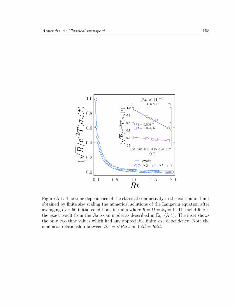
Appendix A: Classical transport 158
0.0 0.5 1.0 1.5 2.0
Rt
0.0
0.2
0.4
0.6
0.8
1.0
(√R
/e∗2
T)σ
cl(t
)
exact∆x → 0,∆t → 0
0.00 0.05 0.10 0.15 0.20 0.25
∆x
0.5
0.6
0.7
0.8
0.9
1.0
(√R
/e∗2
T)σ
cl(t
)t = 0.000t = 0.024/R
0 4 6 8 12 24∆t × 10−3
0.5
0.6
0.7
0.8
0.9
1.0
Figure A.1: The time dependence of the classical conductivity in the continuum limitobtained by finite size scaling the numerical solutions of the Langevin equation afteraveraging over 50 initial conditions in units where ! = D = kB = 1. The solid line isthe exact result from the Gaussian model as described in Eq. (A.4). The inset showsthe only two time values which had any appreciable finite size dependency. Note thenonlinear relationship between ∆x =
√R∆x and ∆t = R∆t.

Appendix B
The Fluctuation Propagator
In this appendix, we will provide details on various results related to the evaluationof the fluctuation propagator at both zero and finite temperatures.
B.1 T = 0
At zero temperature, and coupling g the fluctuation propagator is given by
Π0(k,ω, r) =
∫dq
2π
∫dε
2π
1
(q2 + |ε| + r)[(k + q)2 + |ω + ε| + r]. (B.1)
The momentum and frequency integrals can be done by employing Feynman param-eters to yield
Π0(k,ω, r) =1
2π
1∫
0
dx1
2x− 1
(x
√(k2 − |ω|)x− k2x2 + |ω|
+x− 1
√(k2 + |ω|)x− k2x2
)
=1
2π|k|
[
asin
(k2 + |ω|
√(k2 + |ω|)2 + 4k2r
)
+ asin
(k2 − |ω|
√(k2 + |ω|)2 + 4k2r
)]
+1
2π√
k2 + 2|ω|+ 4r
Re
[
atanh
(k2 + 3|ω| + 4r
2√
k2 + 2|ω| + 4r√
r + |ω|
)]
− Re
[
atanh
(k2 + |ω| + 4r
2√
k2 + 2|ω|+ 4r√
r
)]
. (B.2)
Using the relation
Re [atanh(z)] =1
2ln
∣∣∣∣1 + z
1− z
∣∣∣∣ (B.3)
159
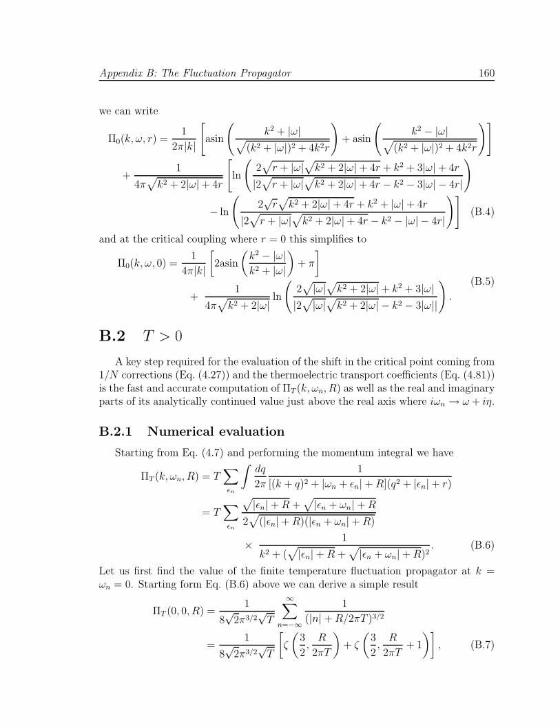
Appendix B: The Fluctuation Propagator 160
we can write
Π0(k,ω, r) =1
2π|k|
[
asin
(k2 + |ω|
√(k2 + |ω|)2 + 4k2r
)
+ asin
(k2 − |ω|
√(k2 + |ω|)2 + 4k2r
)]
+1
4π√
k2 + 2|ω| + 4r
[
ln
(2√
r + |ω|√
k2 + 2|ω| + 4r + k2 + 3|ω|+ 4r
|2√
r + |ω|√
k2 + 2|ω|+ 4r − k2 − 3|ω|− 4r|
)
− ln
(2√
r√
k2 + 2|ω|+ 4r + k2 + |ω|+ 4r
|2√
r + |ω|√
k2 + 2|ω|+ 4r − k2 − |ω|− 4r|
)]
(B.4)
and at the critical coupling where r = 0 this simplifies to
Π0(k,ω, 0) =1
4π|k|
[2asin
(k2 − |ω|k2 + |ω|
)+ π
]
+1
4π√
k2 + 2|ω|ln
(2√|ω|√
k2 + 2|ω| + k2 + 3|ω||2√|ω|√
k2 + 2|ω|− k2 − 3|ω||
)
.
(B.5)
B.2 T > 0
A key step required for the evaluation of the shift in the critical point coming from1/N corrections (Eq. (4.27)) and the thermoelectric transport coefficients (Eq. (4.81))is the fast and accurate computation of ΠT (k,ωn, R) as well as the real and imaginaryparts of its analytically continued value just above the real axis where iωn → ω + iη.
B.2.1 Numerical evaluation
Starting from Eq. (4.7) and performing the momentum integral we have
ΠT (k,ωn, R) = T∑
εn
∫dq
2π
1
[(k + q)2 + |ωn + εn| + R](q2 + |εn| + r)
= T∑
εn
√|εn| + R +
√|εn + ωn| + R
2√
(|εn| + R)(|εn + ωn| + R)
×1
k2 + (√|εn| + R +
√|εn + ωn| + R)2
. (B.6)
Let us first find the value of the finite temperature fluctuation propagator at k =ωn = 0. Starting form Eq. (B.6) above we can derive a simple result
ΠT (0, 0, R) =1
8√
2π3/2√
T
∞∑
n=−∞
1
(|n| + R/2πT )3/2
=1
8√
2π3/2√
T
[ζ
(3
2,
R
2πT
)+ ζ
(3
2,
R
2πT+ 1
)], (B.7)

Appendix B: The Fluctuation Propagator 161
where ζ(a, x) is the Hurwitz zeta function. In order to evaluate the sum in Eq. (B.6)at finite frequencies and wavevectors, we explicitly sum the terms up to some largevalue of |εn| < 2πL where 2πL. |ωn|. For the remaining terms, we perform a seriesexpansion of the summand in powers of 1/|εn| and then use the asymptotic series
∞∑
n=L
1
ns=
L−s+1
Γ(s)
∞∫
0
ys−2e−ydy
1− e−s/L
= L−s+1
[1
s− 1+
1
2L+
s
12L2−
Γ(s + 3)
720Γ(s)L4+
Γ(s + 5)
30240Γ(s)L6
−Γ(s + 7)
1209600Γ(s)L8+
Γ(s + 9)
47900160Γ(s)L10+ . . .
]
. (B.8)
As discussed in Ref. [127], we must use the value of R given in Eq. (4.18) for theresulting ΠT (k,ωn, R) to be well behaved at large k and ωn.
B.2.2 Re [ΠT (q,Ω, R)]−1
Here we provide details on the use of the summation formulas described in Ap-pendix C to evaluate the real and imaginary parts of the fluctuation propagatoranalytically continued to real frequencies. Again, we start from
ΠT (q,Ωn, R) = T∑
εn
∫dk
2π
1
(k2 + R + |εn|)[(k + q)2 + R + |εn + Ωn|](B.9)
and need to analytically continue to real frequencies iΩn → Ω + iη. Thus, usingEq. (C.3) we perform the Matsubara summation to give
ΠT (q,Ω + iη, R) =1
2
∫dk
2π
∫dε
2π
coth( ε
2T
) [FΠ(q, k, ε+ iη, ε+ Ω + iη)
− FΠ(q, k, ε− iη, ε+ Ω + iη)]
+ coth
(ε+ Ω
2T
)[FΠ(q, k, ε− iη, ε+ Ω + iη)
− FΠ(q, k, ε− iη, ε+ Ω− iη]
(B.10)
where
FΠ(q, k, ε± iη, ν ± iη) =1
(k2 + R∓ iε)[(k + q)2 + R∓ iν]. (B.11)

Appendix B: The Fluctuation Propagator 162
Considering each of the four terms in Eq. (B.10) separately, we will have to performan integral of the form
IΠ(q, a, b) =
∫dk
2π
1
(k2 + a)[(k + q)2 + b]=
1
2
(1√a
+1√b
)1
q2 + (√
a +√
b)2(B.12)
which was evaluated using Feynman parameters and in the particular case consideredhere Re a = Re b = R > 0.
We will use the fact that
1√a∓ ib
=1√
2√
a2 + b2
(√√a2 + b2 + a ± i sgn(b)
√√a2 + b2 − a
)(B.13)
and
Re1
q2 + (√
a− iζbb +√
a− iζcc)2=
1
∆(q, a, b, ζb, c, ζc)
[
q2 + 2a +√
(√
a2 + b2 + a)(√
a2 + c2 + a)
− ζbζc sgn(b) sgn(c)√
(√
a2 + b2 − a)(√
a2 + c2 − a)
]
(B.14a)
Im1
q2 + (√
a− iζbb +√
a− iζcc)2=
1
∆(q, a, b, ζb, c, ζc)
[
ζbb + ζcc + ζc sgn(c)√
(√
a2 + b2 + a)(√
a2 + c2 − a)
+ ζb sgn(b)√
(√
a2 + b2 − a)(√
a2 + c2 + a)
]
(B.14b)
where
∆(q, a, b, ζb, c, ζc) =
[
q2 + 2a +√
(√
a2 + b2 + a)(√
a2 + c2 + a)
− ζbζc sgn(b) sgn(c)√
(√
a2 + b2 − a)(√
a2 + c2 − a)
]2
+
[
ζbb + ζcc + ζc sgn(c)√
(√
a2 + b2 + a)(√
a2 + c2 − a)
+ ζb sgn(b)√
(√
a2 + b2 − a)(√
a2 + c2 + a)
]2
(B.15)

Appendix B: The Fluctuation Propagator 163
with a, b, c ∈ R and ζb,c = ±1.Therefore, using Eq. (B.12) to Eq. (B.15) we can write the real and imaginary parts
of the analytically continued fluctuation propagator as (suppressing all R dependence)
ReΠT (q,Ω± iη) =1
2
∫dε
2π
coth( ε
2T
)Im fΠ(q, ε+ iη, ε+ Ω + iη)
− coth
(ε+ Ω
2T
)Im fΠ(q, ε− iη, ε+ Ω− iη)
+
[coth
(ε+ Ω
2T
)− coth
( ε2T
)]Im fΠ(q, ε− iη, ε+ Ω + iη)
(B.16a)
ImΠT (q,Ω± iη) = ∓1
2
∫dε
2π
coth( ε
2T
)Re fΠ(q, ε+ iη, ε+ Ω + iη)
− coth
(ε+ Ω
2T
)Re fΠ(q, ε− iη, ε+ Ω− iη)
+
[coth
(ε+ Ω
2T
)− coth
( ε2T
)]Re fΠ(q, ε− iη, ε+ Ω + iη)
(B.16b)
with
Re fΠ(q, ε+ iζεη, ν + iζνη) =
1
2√
2∆(q, R, ε, ζε, ν, ζν)
(√√R2 + ε2 + R√R2 + ε2
+
√√R2 + ν2 + R√R2 + ν2
)
×[q2 + 2R +
√(√
R2 + ε2 + R)(√
R2 + ν2 + R)
− ζεζν sgn(ε) sgn(ν)√
(√
R2 + ε2 − R)(√
R2 + ν2 −R)
]
−
(
ζε sgn(ε)
√√R2 + ε2 −R√R2 + ε2
+ ζν sgn(ν)
√√R2 + ν2 − R√R2 + ν2
)
×[ζεε+ ζνν + ζν sgn(ν)
√(√
R2 + ε2 + R)(√
R2 + ν2 −R)
+ ζε sgn(ε)√
(√
R2 + ε2 − R)(√
R2 + ν2 + R)
]
(B.17a)

Appendix B: The Fluctuation Propagator 164
and
Im fΠ(q, ε+ iζεη, ν + iζνη) =
1
2√
2∆(q, R, ε, ζε, ν, ζν)
(
ζε sgn(ε)
√√R2 + ε2 −R√R2 + ε2
+ ζν sgn(ν)
√√R2 + ν2 − R√R2 + ν2
)
×[q2 + 2R +
√(√
R2 + ε2 + R)(√
R2 + ν2 + R)
− ζεζν sgn(ε) sgn(ν)√
(√
R2 + ε2 − R)(√
R2 + ν2 −R)
]
+
(√√R2 + ε2 + R√R2 + ε2
+
√√R2 + ν2 + R√R2 + ν2
)
×[ζεε+ ζνν + ζν sgn(ν)
√(√
R2 + ε2 + R)(√
R2 + ν2 −R)
+ ζε sgn(ε)√
(√
R2 + ε2 − R)(√
R2 + ν2 + R)
]
, (B.17b)
where ζε,ν = ±1. Such a formulation allows us to compute both the real and imaginaryparts of ΠT without having to resort to a Kramers-Kronig relation, leading to
Re
[1
ΠT (q,Ω, R)
]=
ReΠT (q,Ω, R)
[ReΠT (q,Ω, R)]2 + [ImΠT (q,Ω, R)]2. (B.18)

Appendix C
Details on the Evaluation ofMatsubara Sums
We begin with the basic identity [128]
T∑
εn
F(iεn) =1
2
∞∫
−∞
dε
2πicoth
( ε2T
)[F (ε+ iη)− F (ε− iη)] , (C.1)
noting that if F (iεn) = F(|εn|), then after analytic continuation F (ε± iη) = F(∓iε).By a similar application of contour integration we obtain
I2(iωn) = T∑
εn
F(iεn, i(εn + ωn))
=1
2
∞∫
−∞
dε
2πicoth
( ε2T
) [F (ε+ iη, ε+ iωn)− F (ε− iη, ε+ iωn)
+ F (ε− iωn, ε+ iη)− F (ε− iωn, ε− iη)]
(C.2)
and so
I2(ω + iη) =
∞∫
−∞
dε
2πi
coth( ε
2T
) [F (ε+ iη, ε+ ω + iη)− F (ε− iη, ε+ ω + iη)
]
+ coth
(ε+ ω
2T
)[F (ε− iη, ε+ ω + iη)− F (ε− iη, ε+ ω − iη)
]
=
∞∫
−∞
dε
2πi
coth( ε
2T
) [F (++)− F (−+)
]
+ coth
(ε+ ω
2T
)[F (−+)− F (−−)
]
(C.3)
165

Appendix C: Details on the Evaluation of Matsubara Sums 166
where in the last expression we only denote the sign of the iη term, because thefrequency arguments remain the same in all terms:
F (±±) ≡ F (ε± iη, ε+ ω ± iη). (C.4)
Rearranging the terms to preserve the order of the frequency arguments will allow usto pull out common factors in the numerator and lead to many simplifications.
Any corrections coming from the presence of a finite self energy at order 1/Nrequire that we perform a dual Matsubara summation over a function with fourfrequency arguments. Through a further generalization of the method of contourintegration used to obtain Eq. (C.2 we find
I4(iωn) = T 2∑
εn,Ωn
F(iεn, iΩn, i(εn + Ωn), i(εn + ωn))
= T∑
εn
1
2
∞∫
−∞
dΩ
2πicoth
(Ω
2T
)[F (iεn,Ω + iη,Ω + iεn, i(εn + ωn))
− F (iεn,Ω− iη,Ω + iεn, i(εn + ωn))
+ F (iεn,Ω− iεn,Ω + iη, i(εn + ωn)) (C.5)
− F (iεn,Ω− iεn,Ω− iη, i(εn + ωn))]
=1
4
∞∫
−∞
dΩ
2πicoth
(Ω
2T
) ∞∫
−∞
dε
2πicoth
( ε2T
)
×[Υ+
4 (ε,Ω, iωn; iη)−Υ−4 (ε,Ω, iωn; iη)
](C.6)
where
Υ+4 (ε,Ω, iωn; iη) = F (ε+ iη,Ω + iη,Ω + ε+ iη, ε+ iωn)
+ F (ε+ iη,Ω− ε− iη,Ω + iη, ε+ iωn) + F (ε− iη,Ω− iη,Ω + ε− iη, ε+ iωn)
+ F (ε− iη,Ω− ε+ iη,Ω− iη, ε+ iωn) + F (ε− iωn,Ω + iη,Ω + ε− iωn, ε+ iη)
+ F (ε− iωn,Ω− ε+ iωn,Ω + iη, ε+ iη) + F (ε− iωn,Ω− iη,Ω + ε− iωn, ε− iη)
+ F (ε− iωn,Ω− ε+ iωn,Ω− iη, ε− iη) (C.7)
and
Υ−4 (ε,Ω, iωn; iη) = F (ε+ iη,Ω− iη,Ω + ε+ iη, ε+ iωn)
+ F (ε+ iη,Ω− ε− iη,Ω− iη, ε+ iωn) + F (ε− iη,Ω + iη,Ω + ε− iη, ε+ iωn)
+ F (ε− iη,Ω− ε+ iη,Ω + iη, ε+ iωn) + F (ε− iωn,Ω− iη,Ω + ε− iωn, ε+ iη)
+ F (ε− iωn,Ω− ε+ iωn,Ω− iη, ε+ iη) + F (ε− iωn,Ω + iη,Ω + ε− iωn, ε− iη)
+ F (ε− iωn,Ω− ε+ iωn,Ω + iη, ε− iη)
Appendix C: Details on the Evaluation of Matsubara Sums 167
so that
I4(ω + iη) =1
4
∞∫
−∞
dΩ
2πi
∞∫
−∞
dε
2πi
×
coth
(Ω
2T
)coth
( ε2T
) [F (+ + ++)− F (+−++)
+ F (−−−+)− F (−+−+)]
+ coth
(Ω + ε
2T
)coth
( ε2T
) [F (+−++)− F (+−−+)
+ F (−+−+)− F (−+ ++)]
+ coth
(Ω
2T
)coth
(ε+ ω
2T
)[F (−+−+)− F (−−−+)
+ F (−−−−)− F (−+−−)]
+ coth
(Ω + ε
2T
)coth
(ε+ ω
2T
)[F (−+ ++)− F (−+−+)
+ F (−+−−)− F (−+ +−)]
. (C.8)
Multiple change of variable transformations have been performed to ensure that thefunction F in the terms above have the same arguments ε, Ω, ε+ Ω, ε+ ω, and thusonly the signs of the iη terms have been denoted,
F (±±±±) = F (ε± iη,Ω± iη, ε+ Ω± iη, ε+ ω ± iη). (C.9)
Finally, the vertex corrections are similar in that we still need to perform a dualMatsubara sum, but now the frequency arguments are more complicated, and there
Appendix C: Details on the Evaluation of Matsubara Sums 168
are five unique combinations
I5(iωn) = T 2∑
εn,Ωn
F(iεn, i(εn + ωn), iΩn, i(Ωn + ωn), i(Ωn − εn))
= T∑
εn
1
2
∞∫
−∞
dΩ
2πicoth
(Ω
2T
)
×[F (iεn, i(εn + ωn),Ω + iη,Ω + iωn,Ω− iεn)
− F (iεn, i(εn + ωn),Ω− iη,Ω + iωn,Ω− iεn)
+ F (iεn, i(εn + ωn),Ω− iωn,Ω + iη,Ω− iεn − iωn)
− F (iεn, i(εn + ωn),Ω− iωn,Ω− iη,Ω− iεn − iωn)
+ F (iεn, i(εn + ωn),Ω + iεn,Ω + iωn + iεn,Ω + iη)
− F (iεn, i(εn + ωn),Ω + iεn,Ω + iωn + iεn,Ω− iη)]
=1
4
∞∫
−∞
dΩ
2πicoth
(Ω
2T
) ∞∫
−∞
dε
2πicoth
( ε2T
)
×[Υ+
5 (ε,Ω, iωn; iη)−Υ−5 (ε,Ω, iωn; iη)
](C.10)
where
Υ+5 (ε,Ω, iωn; iη) = F (ε+ iη, ε+ iωn,Ω + iη,Ω + iωn,Ω− ε− iη)
+ F (ε+ iη, ε+ iωn,Ω− iωn,Ω + iη,Ω− ε− iωn)
+ F (ε+ iη, ε+ iωn,Ω + ε+ iη,Ω + iωn + ε,Ω + iη)
+ F (ε− iη, ε+ iωn,Ω− iη,Ω + iωn,Ω− ε+ iη)
+ F (ε− iη, ε+ iωn,Ω− iωn,Ω− iη,Ω− ε− iωn)
+ F (ε− iη, ε+ iωn,Ω + ε− iη,Ω + iωn + ε,Ω− iη)
+ F (ε− iωn, ε+ iη,Ω + iη,Ω + iωn,Ω− ε+ iωn)
+ F (ε− iωn, ε+ iη,Ω− iωn,Ω + iη,Ω− ε− iη)
+ F (ε− iωn, ε+ iη,Ω + ε− iωn,Ω + ε+ iη,Ω + iη)
+ F (ε− iωn, ε− iη,Ω− iη,Ω + iωn,Ω− ε+ iωn)
+ F (ε− iωn, ε− iη,Ω− iωn,Ω− iη,Ω− ε+ iη)
+ F (ε− iωn, ε− iη,Ω + ε− iωn,Ω + ε− iη,Ω− iη) (C.11)
Appendix C: Details on the Evaluation of Matsubara Sums 169
and
Υ−5 (ε,Ω, iωn; iη) = F (ε+ iη, ε+ iωn,Ω− iη,Ω + iωn,Ω− ε− iη)
+ F (ε+ iη, ε+ iωn,Ω− iωn,Ω− iη,Ω− ε− iωn)
+ F (ε+ iη, ε+ iωn,Ω + ε+ iη,Ω + iωn + ε,Ω− iη)
+ F (ε− iη, ε+ iωn,Ω + iη,Ω + iωn,Ω− ε+ iη)
+ F (ε− iη, ε+ iωn,Ω− iωn,Ω + iη,Ω− ε− iωn)
+ F (ε− iη, ε+ iωn,Ω + ε− iη,Ω + iωn + ε,Ω + iη)
+ F (ε− iωn, ε+ iη,Ω− iη,Ω + iωn,Ω− ε+ iωn)
+ F (ε− iωn, ε+ iη,Ω− iωn,Ω− iη,Ω− ε− iη)
+ F (ε− iωn, ε+ iη,Ω + ε− iωn,Ω + ε+ iη,Ω− iη)
+ F (ε− iωn, ε− iη,Ω + iη,Ω + iωn,Ω− ε+ iωn)
+ F (ε− iωn, ε− iη,Ω− iωn,Ω + iη,Ω− ε+ iη)
+ F (ε− iωn, ε− iη,Ω + ε− iωn,Ω + ε− iη,Ω + iη). (C.12)
Again performing multiple variable shifts yields a much simpler expression where thefrequency arguments of each term are the same. Suppressing the frequency depen-

Appendix C: Details on the Evaluation of Matsubara Sums 170
dence of I5 = I5(ω + iη) we have
I5 =1
4
∞∫
−∞
dΩ
2πi
∞∫
−∞
dε
2πi
×
coth
(Ω
2T
)coth
( ε2T
) [F (+ + + + +)− F (+ + + +−)
+ F (−+−+−)− F (−+−+ +)]
+ coth
(Ω + ε
2T
)coth
( ε2T
) [F (+ + + +−)− F (+ +−+−)
+ F (−+−+ +)− F (−+ + + +)]
+ coth
(Ω + ε+ ω
2T
)coth
( ε2T
) [F (+ +−+−)− F (+ +−−−)
+ F (−+−−−)− F (−+−+−)]
+ coth
(Ω + ε
2T
)coth
(ε+ ω
2T
)[F (−+ + + +)− F (−+−+ +)
+ F (−−−+ +)− F (−−+ + +)]
+ coth
(Ω + ε+ ω
2T
)coth
(ε+ ω
2T
)[F (−+−+−)− F (−+−−−)
+ F (−−−−+) + F (−−−+ +)]
+ coth
(Ω
2T
)coth
(ε+ ω
2T
)[F (−+−+ +)− F (−+−+−)
+ F (−−−−−) + F (−−−−+)]
(C.13)
where the arguments of F have been shifted to be ε, ε+ ω, ε+ Ω, ε+ Ω + ω, Ω,
F (±,±,±,±,±) ≡ F (ε± iη, ε+ ω ± iη, ε+ Ω± iη, ε+ Ω + ω ± iη,Ω± iη). (C.14)

Appendix D
Susceptibility Scaling
In this appendix, we derive scaling forms for the average and local dynamical orderparameter susceptibilities by appealing to the physical picture provided by the strongdisorder renormalization group [129, 152]. In the presence of flow to infinite random-ness, averages of physical quantities in the Griffiths phase will be dominated by rareregions that are strongly ordered. The susceptibility will feel a maximal contributionfrom the small number of clusters with abnormally small eigenvalues, thus we beginby considering the action of a single cluster at zero temperature characterized byorder parameter Ψ
Sclust =
∫dω
2πΨ∗(ω)(r + γ0|ω|)Ψ(ω) (D.1)
where γ0 measures the bare strength of the Ohmic dissipation. The renormalizeddistance from criticality, r, can be found by solving
⟨|Ψ(τ)|2
⟩Sclust
= 1. (D.2)
Adding a source term and taking the suitable derivative we find
χclust(iω) =1
r + γ0|ω|(D.3)
or analytically continuing to real frequencies
Imχclust(ω) =γ0ω
r2 + γ20ω2
. (D.4)
The above analysis neglects fluctuations within a cluster, and to compensate wedefine the average moment of a cluster fluctuating with frequency ω to be µ(ω).Then from simple dimensional considerations, the renormalized single cluster contri-bution to the total susceptibility will be µ2 Imχclust for the average susceptibility and
171

Appendix D: Susceptibility Scaling 172
µ Imχclust for the local susceptibility:
Imχclust(ω) ∼µ2γω
r2 + γ2ω2(D.5a)
Imχclustloc (ω) ∼
µγω
r2 + γ2ω2(D.5b)
where γ = µγ0 has been renormalized due to the modified coupling between joinedclusters and the bath (see for example Eq. (5.4) which describes how the momentrenormalizes under cluster creation). In order to determine the total susceptibilities,the RG procedure is run down to an energy scale Ω = γ0µ(Ω)ω where µ(Ω) is thetypical moment at frequency Ω/! as a result of the narrow distribution of moments.The clusters that get eliminated while reducing the energy scale are strongly fluctuat-ing and do not significantly contribute to the susceptibility. In fact, the only clustersthat contribute will have r * Ω so we have
Imχclust(ω) ∼µ2(Ω)γ0µ(Ω)ω
γ20µ
2(Ω)ω2=
µ(Ω)
ω(D.6a)
Imχclustloc (ω) ∼
µ(Ω)γ0µ(Ω)ω
γ20µ2(Ω)ω2
=1
ω. (D.6b)
Now, performing a summation over all clusters in the sample which contribute atthe energy scale Ω, we find that the total susceptibility is given by the results above,modified by a factor of n(Ω), the density of surviving clusters
Imχ(ω) ∼µ(Ω)n(Ω)
ω(D.7a)
Imχloc(ω) ∼n(Ω)
ω(D.7b)
which can be investigated for δ = 0 at criticality and δ > 0 in the disordered phase.
D.1 δ = 0
Right at criticality, many results are known exactly from Fisher’s solution of theRTFIM [64, 65] and specifically
n(Ω) = | lnΩ |−1/ψ (D.8)
µ(Ω) = | lnΩ |φ (D.9)
where ψ = 1/2 is the tunneling exponent and φ = (1 +√
5)/2 is the cluster exponentfor the RTFIM. When δ = 0, we can set Ω + !ω as corrections coming from µ(Ω) are
Appendix D: Susceptibility Scaling 173
beyond scaling. Substituting into Eqs. (D.7a) and (D.7b) we find
Imχ(ω) ∼| lnω |φ−1/ψ
ω(D.10a)
Imχloc(ω) ∼| lnω |−1/ψ
ω(D.10b)
and thus their ratio scales like the fluctuating cluster moment
R(ω) =Imχ(ω)
Imχloc(ω)∼ | lnω |φ . (D.11)
This was the expected result, as physically argued in Section 5.4.3 or as can be seenfrom an examination of Eq. (D.7a) and (D.7b).
D.2 δ > 0
In the quantum Griffiths phase we expect that δνψ | lnω |. 1 where ν = 2 is thecorrelation length exponent for the RTFIM, Eqs. (D.8) and (D.9) have the modifiedform [65, 153, 137]
n(Ω) ∼ Ωδ/ψδ1/ψ (D.12)
µ(Ω) ∼ δνψ(1−φ) | lnΩ | (D.13)
and now we must use the fact that Ω = γ0µ(Ω)ω which yields
n(Ω) ∼ ωδ/ψδ1/ψ−φνδ(δνψ | lnω |δ/ψ
)(D.14)
µ(Ω) ∼ δ−νψφ(δνψ | lnω |
). (D.15)
Combining these results with Eq. (D.7a) and (D.7b) we find the scaling expressionsin the Griffiths phase
Imχ(ω) ∼δ1/ψ−φνψ(1+1/z)
(δνψ | lnω |
)1−1/z
ω1−1/z(D.16a)
Imχloc(ω) ∼δ1/ψ−φνδ
(δνψ | lnω |
)1/z
ω1−1/z(D.16b)
where we have identified z ≡ ψ/δ as an effective dynamic exponent. These scalingforms are confirmed in Figs. 5.9 and 5.10. Their ratio is given by
R(ω) =Imχ(ω)
Imχloc(ω)∼ δ−φνψ
(δνψ | lnω |
)(D.17)
and the existence of this scaling form was essential in our numerical computation ofthe exponent φ in Section 5.4.3.

References
[1] R. Feynman, There is plenty of room at the bottom,http://www.its.caltech.edu/ feynman/plenty.html, 1959.
[2] T. Newman, K. Williams, and R. Pease, J. Vac. Sci. Tech. B 5, 88 (1987).
[3] C. Hirjibehedin, C. Lutz, and A. Heinrich, Science 312, 1021 (2006).
[4] H. Onnes, Comm. Phys. Lab. Univ. Leiden 122, 124 (1911).
[5] W. Meissner and R. Ochsenfeld, Naturwissenschaften 21, 787 (1933).
[6] M. Tinkham, Introduction to Superconductivity (McGraw-Hill, New York,1996).
[7] J. Bednorz and K. Muller, Z. Phys. B 64, 189 (1986).
[8] P. Dai, B. Chakoumakos, G. Sun, K. Wong, Y. Xin, and D. Lu, Physica C 243,201 (1995).
[9] W. S. Corak, B. B. Goodman, C. B. Satterthwaite, and A. Wexler, Phys. Rev.96, 1442 (1954).
[10] L. N. Cooper, Phys. Rev. 104, 1189 (1956).
[11] E. Maxwell, Phys. Rev. 78, 477 (1950).
[12] C. A. Reynolds, B. Serin, W. H. Wright, and L. B. Nesbitt, Phys. Rev. 78, 487(1950).
[13] J. Bardeen, L. N. Cooper, and J. R. Schrieffer, Phys. Rev. 108, 1175 (1957).
[14] N. Nagaosa, Quantum Field Theory in Condensed Matter Physics (Springer,Berlin, 1999).
[15] P. de Gennes, Superconductivity of Metals and Alloys (Perseus Books Group,New York, 1999).
174

References 175
[16] W. W. Webb and R. J. Warburton, Phys. Rev. Lett. 20, 461 (1968).
[17] J. Bardeen, Rev. Mod. Phys. 34, 667 (1962).
[18] W. A. Little, Phys. Rev. 156, 396 (1967).
[19] J. S. Langer and V. Ambegaokar, Phys. Rev. 164, 498 (1967).
[20] D. E. McCumber and B. I. Halperin, Phys. Rev. B 1, 1054 (1970).
[21] N. D. Mermin and H. Wagner, Phys. Rev. Lett. 17, 1133 (1966).
[22] P. C. Hohenberg, Phys. Rev. 158, 383 (1967).
[23] R. Landauer, IBM J. Res. Dev. 44, 251 (2000).
[24] L. Gor’kov, Soviet Phys. JETP 9, 1364 (1959).
[25] B. Josephson, Phys. Lett. 1, 251 (1962).
[26] D. E. McCumber, Phys. Rev. 172, 427 (1968).
[27] A. Schmid, Phys. Rev. Lett. 51, 1506 (1983).
[28] N. Giordano, Phys. Rev. Lett. 61, 2137 (1988).
[29] N. Giordano, Physica B 203, 460 (1994).
[30] A. O. Caldeira and A. J. Leggett, Phys. Rev. Lett. 46, 211 (1981).
[31] J.-M. Duan, Phys. Rev. Lett. 74, 5128 (1995).
[32] A. D. Zaikin, D. S. Golubev, A. van Otterlo, and G. T. Zimanyi, Phys. Rev.Lett. 78, 1552 (1997).
[33] A. Zaikin, D. Golubev, A. van Otterlo, and G. Zimanyi, Usp. Fiz. Nauk. 41,226 (1998).
[34] D. Golubev and A. Zaikin, Phys. Rev. B 64, 14504 (2001).
[35] A. Bezryadin, C. Lau, and M. Tinkham, Nature 404, 971 (2000).
[36] A. Bezryadin, NanoGallery, http://www.nanogallery.info, 2004.
[37] A. Rogachev, T.-C. Wei, D. Pekker, A. T. Bollinger, P. M. Goldbart, and A.Bezryadin, Phys. Rev. Lett. 97, 137001 (2006).
[38] C. N. Lau, N. Markovic, M. Bockrath, A. Bezryadin, and M. Tinkham, Phys.Rev. Lett. 87, 217003 (2001).
References 176
[39] F. Altomare, A. Chang, M. Melloch, Y. Hong, and C. Tu, Phys. Rev. Lett. 97,17001 (2006).
[40] A. Bollinger, R. Dinsmore, A. Rogachev, and A. Bezryadin, arXiv:0707.4532(2008).
[41] A. Abrikosov and L. Gorkov, Sov. Phys. JETP 12, 1243 (1961).
[42] P. Anderson, J. Phys. Chem. Solids 11, 2 (1959).
[43] B. Spivak, A. Zyuzin, and M. Hruska, Phys. Rev. B 64, 132502 (2001).
[44] A. Rogachev, A. T. Bollinger, and A. Bezryadin, Phys. Rev. Lett. 94, 017004(2005).
[45] Y. Liu, Y. Zadorozhny, M. Rosario, B. Rock, P. Carrigan, and H. Wang, Science294, 2332 (2001).
[46] W. A. Little and R. D. Parks, Phys. Rev. Lett. 9, 9 (1962).
[47] J. A. Hertz, Phys. Rev. B 14, 1165 (1976).
[48] S. Sachdev, Quantum Phase Transitions (Cambridge University Press, NewYork, 1999).
[49] T. Vojta, in Computational Statistical Physics, edited by K. Hoffmann and M.Schreiber (Springer, Berlin, 2002).
[50] T. Vojta, arXiv:0709.0964 (2007).
[51] S. L. Sondhi, S. M. Girvin, J. P. Carini, and D. Shahar, Rev. Mod. Phys. 69,315 (1997).
[52] N. Goldenfeld, Lectures on Phase Transitions and the Renormalization Group(Westview Press, New York, 1992).
[53] H. Stanley, Introduction to Phase Transitions and Critical Phenomena (OxfordUniversity Press, New York, 1971).
[54] J. Negle and H. Orland, Quantum Many-Particle Systems (Addison-Wesley,New York, 1988).
[55] J. Cardy, Scaling and renormalization in statistical physics (Cambridge Univer-sity Press, Cambridge, England, 1996).
[56] G. Grinstein, in Fundamental Problems in Statitical Mechanics, edited by E.Cohen (North Holland, Amsterdam, 1985), Vol. VI.

References 177
[57] T. Vojta, J. Phys. A: Math. Gen. 39, R143 (2006).
[58] A. Harris, J. Phys. C 7, 1671 (1974).
[59] C. Holm and W. Janke, Phys. Rev. B 48, 936 (1993).
[60] A. M. Ferrenberg and D. P. Landau, Phys. Rev. B 44, 5081 (1991).
[61] H. G. Ballesteros, L. A. Fernandez, V. Martın-Mayor, A. Munoz Sudupe, G.Parisi, and J. J. Ruiz-Lorenzo, Phys. Rev. B 58, 2740 (1998).
[62] B. M. McCoy and T. T. Wu, Phys. Rev. Lett. 21, 549 (1968).
[63] B. M. McCoy and T. T. Wu, Phys. Rev. 176, 631 (1968).
[64] D. Fisher, Phys. Rev. Lett. 69, 534 (1992).
[65] D. Fisher, Phys. Rev. B 51, 6411 (1995).
[66] K. Binder and A. Young, Rev. Mod. Phys. 58, 801 (1986).
[67] K. Fischer and J. Hertz, Spin Glasses (Cambridge University Press, Cambridge,England, 1991).
[68] D. Sherrington and S. Kirkpatrick, Phys. Rev. Lett. 35, 1792 (1975).
[69] V. Dotsenko, An Introduction to the Theory of Spin Glasses and Neural Net-works (World Scientific, New Jersey, 1994).
[70] R. Griffiths, Phys. Rev. Lett. 23, 17 (1969).
[71] T. Vojta, J. Phys. A: Math. Gen. 36, 10921 (2003).
[72] R. Sknepnek and T. Vojta, Phys. Rev. B 69, 174410 (2004).
[73] G. Schehr and H. Rieger, Phys. Rev. Lett. 96, 227201 (2006).
[74] J. Hoyos and T. Vojta, arXiv:0802.2303 (2008).
[75] S.-k. Ma, C. Dasgupta, and C.-k. Hu, Phys. Rev. Lett. 43, 1434 (1979).
[76] A. Rogachev and A. Bezryadin, Appl. Phys. Lett. 83, 512 (2003).
[77] G. Boogaard, A. Verbruggen, W. Belzig, and T. Klapwijk, Phys. Rev. B 69,220503 (2004).
[78] A. Bollinger, A. Rogachev, and A. Bezryadin, Europhys. Lett. 76, 505 (2006).
[79] R. Ramazashvili and P. Coleman, Phys. Rev. Lett. 79, 3752 (1997).

References 178
[80] I. F. Herbut, Phys. Rev. Lett. 85, 1532 (2000).
[81] V. Galitski, Phys. Rev. B 77, 100502 (2008).
[82] V. Galitski, Phys. Rev. Lett. 100, 127001 (2008).
[83] A. V. Lopatin, N. Shah, and V. M. Vinokur, Phys. Rev. Lett. 94, 037003 (2005).
[84] N. Shah and A. Lopatin, Phys. Rev. B 76, 094511 (2007).
[85] L. Aslamazov and A. Larkin, Sov. Phys. Solid State 10, 1104 (1968).
[86] K. Maki, Prog. Theor. Phys. 40, 193 (1968).
[87] R. Thompson, Phys. Rev. B 1, 327 (1970).
[88] B. Altshuler and A. Aronov, in Electron–Electron Interactions in DisorderedSystems, edited by E. Efros and M. Pollak (North-Holland, Amsterdam, 1985).
[89] S. Sachdev, P. Werner, and M. Troyer, Phys. Rev. Lett. 92, 237003 (2004).
[90] D. Podolsky, A. Vishwanath, J. Moore, and S. Sachdev, Phys. Rev. B 75,014520 (2007).
[91] D. A. Pesin and A. V. Andreev, Phys. Rev. Lett. 97, 117001 (2006).
[92] J. E. Mooij and G. Schon, Phys. Rev. Lett. 55, 114 (1985).
[93] M. V. Feigel’man and A. I. Larkin, Chem. Phys. 235, 107 (1998).
[94] M. V. Feigel’man, A. I. Larkin, and M. A. Skvortsov, Phys. Rev. Lett. 86, 1869(2001).
[95] V. Galitski and A. Larkin, Phys. Rev. Lett. 87, 87001 (2001).
[96] A. Del Maestro, B. Rosenow, N. Shah, and S. Sachdev, Phys. Rev. B 77, 180501(2008).
[97] A. J. Millis, Phys. Rev. B 48, 7183 (1993).
[98] T. Moriya and A. Kawabata, J. Phys. Soc. Jpn. 34, 639 (1973).
[99] S. Pankov, S. Florens, A. Georges, G. Kotliar, and S. Sachdev, Phys. Rev. B69, 054426 (2004).
[100] A. Gamba, M. Grilli, and C. Castellani, Nucl. Phys. B 556, 463 (1999).
[101] P. Werner, M. Troyer, and S. Sachdev, J. Phys. Soc. Jpn. Supl. 74, 67 (2005).

References 179
[102] S. Stintzing and W. Zwerger, Phys. Rev. B 56, 9004 (1997).
[103] H. P. Buchler, V. B. Geshkenbein, and G. Blatter, Phys. Rev. Lett. 92, 067007(2004).
[104] G. Refael, E. Demler, Y. Oreg, and D. S. Fisher, Phys. Rev. B 75, 014522(2007).
[105] D. Meidan, Y. Oreg, and G. Refael, Phys. Rev. Lett. 98, 187001 (2007).
[106] G. Refael, E. Demler, and Y. Oreg, arXiv:0803.2515 (2008).
[107] T. Giamarchi, Phys. Rev. B 46, 342 (1992).
[108] L. B. Ioffe and A. J. Millis, Phys. Rev. B 51, 16151 (1995).
[109] S. Sachdev, A. V. Chubukov, and A. Sokol, Phys. Rev. B 51, 14874 (1995).
[110] J. Tucker and B. Halperin, Phys. Rev. B 3, 3768 (1971).
[111] A. Van Run, J. Romijn, and J. Mooij, Jpn. J. Appl. Phys 26, 1765 (1987).
[112] S. Saito and Y. Murayama, Phys. Lett. A 139, 85 (1989).
[113] N. Shah, D. Pekker, and P. Goldbart, arXiv:0709.3971 (2007).
[114] G. Mahan, Many-Particle Physics (Plenum Publishing Corporation, Boston,2000).
[115] P. Hohenberg and B. Halperin, Rev. Mod. Phys. 49, 435 (1977).
[116] J. Garcıa-Ojalvo and J. Sancho, Noise in Spatially Extended Systems (Springer,New York, 1999).
[117] J. Zinn-Justin, Quantum Field Theory and Critical Phenomena (Oxford Uni-versity Press, New York, 2002).
[118] M. Peskin and D. Schroeder, An Introduction to Quantum Field Theory (PerseusBooks, New York, 1995).
[119] J. Moreno and P. Coleman, cond-mat/9603079 (1996).
[120] D. Fisher and P. Lee, Phys. Rev. B 23, 6851 (1981).
[121] V. Ambegaokar and A. Griffin, Phys. Rev. 137, 1151 (1965).
[122] F. Ronning, R. W. Hill, M. Sutherland, D. G. Hawthorn, M. A. Tanatar, J.Paglione, L. Taillefer, M. J. Graf, R. S. Perry, Y. Maeno, and A. P. Mackenzie,Phys. Rev. Lett. 97, 067005 (2006).

References 180
[123] S. Vishveshwara and M. Fisher, Phys. Rev. B 64, 174511 (2001).
[124] M. Vojta, Y. Zhang, and S. Sachdev, Int. J. Mod. Phys. B 14, 3719 (2000); T.Senthil (unpublished).
[125] M. Li and E. Orignac, Europhys. Lett. 60, 432 (2002).
[126] R. Fazio, F. Hekking, and D. Khmelnitskii, Phys. Rev. Lett. 80, 5611 (1998).
[127] A. V. Chubukov, S. Sachdev, and J. Ye, Phys. Rev. B 49, 11919 (1994).
[128] A. Abrikosov, L. Gorkov, and I. Dzyaloshinski, Methods of Quantum Field The-ory in Statistical Physics (Prentice-Hall, New Jersey, 1963).
[129] J. Hoyos, C. Kotabage, and T. Vojta, Phys. Rev. Lett. 99, 230601 (2007).
[130] D. S. Fisher, Phys. Rev. B 50, 3799 (1994).
[131] C. Dasgupta and S.-k. Ma, Phys. Rev. B 22, 1305 (1980).
[132] G. Refael, S. Kehrein, and D. S. Fisher, Phys. Rev. B 66, 060402 (2002).
[133] J. A. Hoyos and E. Miranda, Phys. Rev. B 69, 214411 (2004).
[134] D. S. Fisher, P. Le Doussal, and C. Monthus, Phys. Rev. Lett. 80, 3539 (1998).
[135] J. Hooyberghs, F. Igloi, and C. Vanderzande, Phys. Rev. Lett. 90, 100601(2003).
[136] J. Hooyberghs, F. Igloi, and C. Vanderzande, Phys. Rev. E 69, 066140 (2004).
[137] F. Igloi and C. Monthus, Phys. Rep. 412, 277 (2005).
[138] O. Motrunich, S.-C. Mau, D. A. Huse, and D. S. Fisher, Phys. Rev. B 61, 1160(2000).
[139] T. Senthil and S. N. Majumdar, Phys. Rev. Lett. 76, 3001 (1996).
[140] A. J. Leggett, S. Chakravarty, A. T. Dorsey, M. P. A. Fisher, A. Garg, and W.Zwerger, Rev. Mod. Phys. 59, 1 (1987).
[141] A. J. Millis, D. K. Morr, and J. Schmalian, Phys. Rev. Lett. 87, 167202 (2001).
[142] A. J. Millis, D. K. Morr, and J. Schmalian, Phys. Rev. B 66, 174433 (2002).
[143] T. Senthil and S. Majumdar, Phys. Rev. Lett. 76, 3001 (1996).
[144] Y. Tu and P. Weichman, Phys. Rev. Lett. 73, 6 (1994).

References 181
[145] J. Hartman and P. Weichman, Phys. Rev. Lett. 74, 4584 (1995).
[146] M. Powell, in Numerical Methods for Nonlinear Algebraic Equations, edited byP. Rabinowitz (Gordon and Breach, New York, 1970).
[147] J. More and M. Cosnard, ACM Trans. Math. Softw. 5, 64 (1979).
[148] A. Young and H. Rieger, Phys. Rev. B 53, 8486 (1996).
[149] T. Vojta and J. Schmalian, Phys. Rev. B 72, 045438 (2005).
[150] O. Motrunich, K. Damle, and D. A. Huse, Phys. Rev. B 63, 134424 (2001).
[151] B. Spivak, P. Oreto, and S. Kivelson, arXiv:0803.2902 (2008).
[152] T. Vojta, “private communication”, 2008.
[153] F. Igloi, Phys. Rev. B 65, 64416 (2002).

![Research Article An FPGA-Based Quantum Computing ...namely, ion trap [ ], nuclear magnetic resonance [ ], and superconductor [ ], were attempted. Nevertheless, only small-scale quantum](https://static.fdocuments.in/doc/165x107/613f7adef0f55d448e4cd24a/research-article-an-fpga-based-quantum-computing-namely-ion-trap-nuclear.jpg)


![arXiv:1307.4403v2 [cond-mat.str-el] 7 Aug 2013 · Universal topological quantum computation from a superconductor/Abelian quantum Hall heterostructure Roger S. K. Mong, 1David J.](https://static.fdocuments.in/doc/165x107/600186f790f11001fe784ae4/arxiv13074403v2-cond-matstr-el-7-aug-2013-universal-topological-quantum-computation.jpg)


