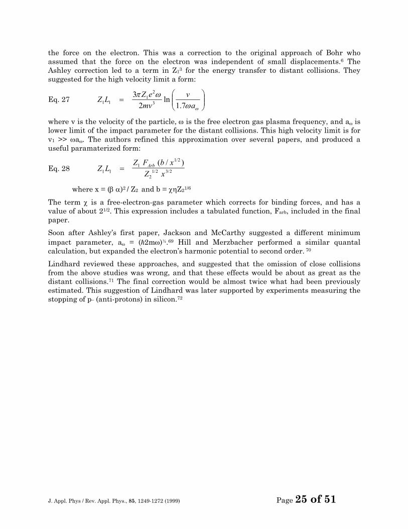
![[1] J. Zhang et al. , Appl. Phys. Lett . 88 , 123112 (2006).](https://static.fdocuments.in/doc/165x107/56815152550346895dbf774f/1-j-zhang-et-al-appl-phys-lett-88-123112-2006.jpg)
[1] J. Zhang et al. , Appl. Phys. Lett . 88 , 123112 (2006).
J. Appl. Phys / Rev. Appl. Phys., 85, 1249-1272 (1999) Page 1 of 51
The Stopping of Energetic Light Ions in Elemental Matter
J. F. Ziegler
J. Appl. Phys / Rev. Appl. Phys., 85, 1249-1272 (1999)
ABSTRACT The formalism for calculating the stopping of energetic light ions (H, He and Li) at energies above 1 MeV/u, has advanced to the point that stopping powers may now be calculated with an accuracy of a few percent for all elemental materials. Although the subject has been of interest for a century, only recently have the final required corrections been understood and evaluated. The theory of energetic ion stopping is reviewed with emphasis on those aspects that pertain to the calculation of accurate stopping powers.
Table of Contents HISTORICAL REVIEW.......................................................................................................1 THE BETHE-BLOCH EQUATION.......................................................................................3
Variations of the Bethe-Bloch Equation.......................................................................6 Low Velocity Limit of the Bethe-Bloch Theory: Particle Neutralization .....................8
THE PRIMARY STOPPING NUMBER, L0...........................................................................9 Shell Corrections, C/Z2...............................................................................................11
Shell Corrections using Hydrogenic Wave Functions ....................................................... 12 Shell Corrections using the Local Density Approximation ............................................... 13 Empirical Summed Shell and Ionization Corrections ........................................................ 15 Comparison of Two Types of Shell Correction Calculations ............................................ 19
Density Effect Correction to L0, δ/2 ...........................................................................21 THE BARKAS CORRECTION, L1 ....................................................................................23
The Barkas Effect from Charge Sign Considerations ................................................24 The Barkas Effect from Charge Magnitude Considerations ......................................26 Theoretical Barkas-Effect Calculations .....................................................................27 Unified Barkas Correction Factor .............................................................................28 Empirical Barkas Correction Term............................................................................30
THE BLOCH CORRECTION, L2 ......................................................................................32 RELATIVE MAGNITUDE OF BETHE-BLOCH CORRECTIONS..........................................36 THE ACCURACY OF CURRENT STOPPING THEORY ......................................................37 APPENDIX .......................................................................................................................40
Stopping Powers using the Local Density Approximation.........................................40 Lindhard Stopping in a Free Electron Gas ................................................................40 Stopping Calculations using Local Density Approximation ......................................43
HISTORICAL REVIEW Soon after the discovery of energetic particle emission from radioactive materials, there was interest in how these corpuscles were slowed down in traversing matter. From her work in
J. Appl. Phys / Rev. Appl. Phys., 85, 1249-1272 (1999) Page 2 of 51
1898-1899, Marie Curie stated the hypothesis that "les rayons alpha sont des projectiles materiels susceptibles de perdre de leur vitesse en traversant la matiere."1 Many scientists immediately realized that since these particles could penetrate thin films, such experiments might finally unravel the secrets of the atom. Early attempts to create a particle energy loss theory were inconclusive for there was not yet an accurate proposed model of the atom. The theoretical treatment for the scattering of two point charges was derived by J. J. Thomson in his classic book on electricity.2 Much of the traditional particle energy-loss symbolism can be traced to this book which introduced a comprehensive treatment for classical Coulombic scattering between energetic charged particles. This work, however, did not attempt to calculate actual stopping powers.
Enough experimental evidence of radioactive particle interactions with matter was collected in the next decade to make stopping power theory one of the central concerns of those attempting to develop an atomic model. In 1909, Geiger and Marsden were studying the penetration of alpha-particles through thin foils, and the spread of the trajectories after emerging from the back side.3 They reported that about .01% of the heavy alpha-particles were scattered backwards from the target, and from an analysis of the data statistics such backscattered events had to be from isolated single collisions. Two years later, Rutherford was able to demonstrate theoretically that the backscattering was indeed due to a single event, and by analyzing this and electron scattering data he was able to first calculate that the nucleus of Al atoms must have a mass of about 22 and platinum would have a mass of 138 !4 J. J. Thomson, director of the prestigious Cavendish Laboratory, and Niels Bohr, a fresh post-doctoral scientist who had left the Cavendish lab for Rutherford's Manchester Laboratory, published almost simultaneously an analysis of the stopping of charged particles by matter.5 These papers illustrate much of their divergent ideas on the model of an atom. Thomson incredibly ignored the alpha-particle backscattering measurements of Geiger3 and the Rutherford heavy-particle scattering theory4 which emphasized the atomic positive charge must be concentrated within the atom. But the nuclear atom with a heavy positively-charged core was the basis of Bohr's ideas.67 Bohr's early work is instructive because for the first time a unified theory of stopping was attempted, and we can see in this and in similar works the essential problems of stopping theory:
• How does an energetic charged particle (a point charge) lose energy to the quantized electron plasma of a solid (inelastic energy loss)?
• How do you incorporate into this interaction simultaneous distortion of the electron plasma caused by the particle (target polarization)?
• How can you extend the point charge-plasma interaction to that for a finite moving atom in a plasma?
• How do you estimate the degree of ionization of the moving atom and describe its electrons when it is both ionized and within an electron plasma?
• How do you calculate the screened Coulomb scattering of the moving atom with each heavy target nucleus it passes?
• How do you include relativistic corrections to all of the above?
This is a brief list of the major problems encountered, and scientific interest shifts back and forth between them over the decades because of external scientific tidal forces such as (a) the development of quantal scattering in the nineteen twenties, (b) the study of nuclear fission in the thirties and forties, (c) the study of nuclear physics in the fifties, (d) the
J. Appl. Phys / Rev. Appl. Phys., 85, 1249-1272 (1999) Page 3 of 51
technological applications of ion implantation for material modification in the sixties, and the use of ion beams in material analysis and in radiation oncology in the seventies. This ebb and flow of interest continues because of the recurrent importance of the problem, and the difficulty of calculating the penetration of energetic atoms in solids from first principles. We briefly review some of the historical milestones in this field below.
One of Bohr's original conclusions was that the energy loss of ions passing through matter could be divided into two components: nuclear stopping (energy loss to the medium's atomic positive cores) and electronic stopping (energy loss to the medium's light electrons). Bohr, in his first papers, correctly deduced that the electronic stopping would be far greater than the nuclear stopping for energetic light ions such as are emitted by radioactive sources. This conclusion was based on recoil kinematics considering only the relative masses and abundance of the target electrons and nuclei. Bohr further introduced atomic structure into stopping theory by giving target electrons the orbital frequencies obtained from optical spectra and calculating the energy transferred to such harmonic oscillators. He noted that the experimentally reported stopping powers for heavy atom targets indicated that many electrons in these targets must be more tightly bound than the optical data suggested. He also realized that his accounting of the energy loss process was seriously limited by a lack of knowledge of the charge state of the ion inside the matter, i.e., its effective charge in its interaction with the target medium.
A major advance in understanding stopping powers came 20 years later when Bethe89 and Bloch1011 restated the problems from the perspective of quantum mechanics, and derived in the Born approximation the fundamental equations for the stopping of very fast particles in a quantized medium. This theoretical approach remains the basic method for evaluating the energy loss of light particles with velocities above 1 MeV/amu.
THE BETHE-BLOCH EQUATION The stopping of high velocity light ions in matter usually assumes two major simplifications in stopping theory: (1) the ion is moving much faster than the target electrons and is fully stripped of its electrons, and (2) the ion is much heavier than the target electrons. In general, this paper will treat light ions (H, He and Li) with energies between 1 MeV/u to 10 GeV/u. Considerations of partial ion neutralization at lower velocities establishes the lower energy limit (see details in the section Low Velocity Limits), while the upper energy limit is constrained by the lack of experimental data.
Extended reviews of the early concepts of Bohr, Bethe and Bloch, with significant additions using quantum-mechanical perturbation treatments, have been written by Fano12-16, Inokuti17, Bichsel18, Sigmund19, Jackson20 and Ahlen21
Relativistic quantum mechanics allows quite different approaches to analyze the transfer of energy from the particle to the medium, and the results of using various theoretical procedures are sometimes difficult to compare. All attempts to create tables of high energy ion stopping powers have required normalization of the theory to experimental data to obtain accurate values (see books by Fano22, Northcliffe23, Janni24, Andersen25, Ziegler26 and the ICRU27).
Bohr's early work evaluated the classical stopping of a fast heavy charged particle to an electron bound in a harmonic potential.6,7 This early work was extended by others who applied quantum mechanics to particle energy loss - of note was the early work by Henderson in 1922, who considered the energy loss by a particle to an atom with quantized
J. Appl. Phys / Rev. Appl. Phys., 85, 1249-1272 (1999) Page 4 of 51
electrons, but ignored distant interactions or any collective excitation of the electronic medium of the target.28 Gaunt, in 1927, applied a quantum mechanical treatment to the perturbation of atomic electrons by a charged particle.29 Unfortunately, Gaunt made an error in one approximation that led to the wrong formula for the particle’s energy loss.30 Bethe presented the first complete solution to high velocity stopping using the first Born approximation where the entire physical system is considered quantized.8 Then Moller31 and Bethe9 extended these ideas by including relativistic corrections.
The following theoretical review will assume the following symbols: Z1 = Particle atomic number
M1 = Particle mass (u) E = Particle energy v = Particle velocity
vo = The Bohr velocity = e2/h = 25 keV/u b = Impact parameter of particle to a target electron
Z2 = Target atomic number M2 = Target atomic weight (u) N = Density of target atoms per unit volume e = Charge of an electron
me = Mass of an electron c = Velocity of light β = Relative particle velocity, v/c
Certain primary assumptions pertain to all theories described. The particle is assumed to interact with the target only through electromagnetic forces. Any energy loss to nuclear reactions between the particle and the target nuclei are ignored. For high velocities, Bethe showed that the ratio of the energy loss by the particle to the target electrons was greater than the loss to the heavier target nuclei by at least M2/meZ2.8 Less than 0.1% of the energy loss of high velocity particles is to the target nuclei (ignoring nuclear reactions). Hence we shall not evaluate the energy loss between the particle and the target nuclei.
With the above assumptions, we can reduce the energy loss problem to one which considers only the energy loss by the high velocity particle to the atomic electrons, which are bound to infinitely heavy nuclei.
There are two basic approaches used to evaluate a particle’s energy loss to target electrons. These are the Bohr approach, which is dependent on the impact parameter between the particle’s trajectory and the target nucleus, and the Bethe approach which depends on momentum transfer from the particle to the target electrons. Bethe’s approach was necessary since quantum mechanics prohibits a particle with a well defined momentum having a spatially localized position. Hence Bohr’s concept of an impact parameter (defined in 1913, before quantum mechanics was developed) could not be directly upgraded to wave mechanics. There was no quantized solution to close collisions if one attempted to use the Bohr impact parameter concepts.
Briefly, the highlights of the Bethe-Bloch theory are described below. The reader is referred to the lengthy tutorials cited in the first paragraph of this paper for extended derivations.
The classical Bohr approach considers an heavy charged particle of charge, Z1e, moving at a velocity, v, passing near a light electron of charge, e, and mass, m, at an impact parameter, b. The transverse momentum impulse, ∆p, to the light electron is:
J. Appl. Phys / Rev. Appl. Phys., 85, 1249-1272 (1999) Page 5 of 51
Eq. 1 ∆p = 2
12)(bv
eZdttEe =∫∞
∞−
where E is the transverse electrical field. The energy transferred is then:
Eq. 2 ∆E = ( )
( )∆p
mZ emv b
21
2 4
2 222 1
=
This expression assumes that the electron does not move much relative to the impact parameter, b. To obtain the stopping power, S, this transferred energy must be integrated over all possible impact parameters, b. Assuming the target is made of atoms of atomic number, Z2. the energy loss per target atom is :
Eq. 3 S Z E b b db= ∫2 2π ∆ ( )
Eq. 4 ∫∞
=0
22
421
214 dbbbvm
eZZπ
The integral of this expression diverges as b → 0, so it is necessary to argue a minimum impact parameter, bmin. If the electron mass is assumed to be very much smaller than the mass of the incident particle, the electron will recoil strongly for very small impact parameters. Noting that the maximum energy transfer is for a head-on collision, we may use Rutherford two-particle elastic scattering to estimate the closest distance of approach for a head-on collision. This gives a minimum distance of bmin ∼ Z1e2/mv2.
The integral also becomes undefined for bmax→ ∞. This can be made tractable by noting that, for distant collisions, if the interaction is long compared to the orbiting frequency of an electron, the collision will become adiabatic and no energy will be transferred. This suggests a cutoff when the collision time becomes longer than the orbital frequency, bmax∼ v/ω, where ω is the orbital frequency.
Inserting these values for bmin and bmax, the energy loss becomes:
Eq. 5
=
ωπ 2
1
3
2
421
2 ln4eZ
mvvmeZZ
dxdE
The relativistic form of this equation is made by equating the particle’s energy, E = γ M1c2, where γ = 1/(1-β2)½ and β=v/c. This expands bmax∼ γv/ω, and bmin ∼ Z1e2/γmv2 and the integral becomes:
Eq. 6
=
ωγπ
21
322
12
42 ln4
eZmvZ
vmeZ
dxdE
Bohr used this expression to form the basis of his evaluation of the energy loss of a heavy particle to a medium of harmonically bound electrons.6
Bloch evaluated the differences between the classical (Bohr) and quantum-mechanical (Bethe) approaches for particles with velocities much larger than the target electrons . He showed that Bohr’s approach was valid also in the quantum mechanics of a bound electron if the energy transferred was assumed to be the mean energy loss, summed over all possible
J. Appl. Phys / Rev. Appl. Phys., 85, 1249-1272 (1999) Page 6 of 51
atomic transitions. However, Bloch needed to assume the dipole approximation (impact parameter >> orbit diameter) to avoid the localization problem discussed above.
Bloch then analyzed the problem of close collisions. He did not assume, as Bethe had done, that it was valid to consider the electrons to be plane waves in the center of momentum frame. Instead, he confined the electrons to the interior of a cylinder, which then introduced transverse momentum components that interfere with one another under the forces of the electromagnetic interaction. This led to quite different momentum transfers than for the case of Bethe’s plane wave scattering.
Bloch then showed that for low momentum transfers, his cylinder confinement radius would be large enough to permit the use of Bethe’s plane-wave approach, and so for these collisions the Bethe approach was correct. Further, for large momentum transfers, the wave packets would scatter classically, and hence the Bohr approach would be valid. Thus Bloch found the bridging formulation between the classical Bohr impact-parameter approach, and the quantized Bethe momentum transfer approach to energy loss. Unfortunately, Bloch made a small error in estimating one scattering cross-section, and his final formula as presented in original the paper contains an error.
The original Bethe-Bloch relativistic stopping formula, S may be stated as:
Eq. 7 Se Z
m vZ
mvI
Ze
=< >
− − − +
4 21
42
2 12
22 2
1
πβ βln ln( ) ( )Ψ
where <I> is the averaged excitation potential per electron, and is defined as
Eq. 8 ln ln< > =∑I f En n
where the logarithm of the mean ionization potential, ln <I>, can be expanded as the dipole oscillator strength for the nth energy level:
Eq. 9 fmE
Zn xn
nj
j= ∑2
022
2
h
Normalization for this sum rule is that Σfn = 1.
The final term, Ψ(Z1) in Eq. 7, is a small term which contains Bloch’s error so that the Bloch result does not reduce to the Bethe result for the limit Z1α/β → 0, where α = the fine structure constant, e2/hc = 1/137.
Variations of the Bethe-Bloch Equation
The theoretical studies of the energy loss of high velocity particles have been active for almost a century. The earliest works which are still quoted are those by J. J. Thomson - 1903, 191232, E. Rutherford - 191133 and N. Bohr - 191334. There are many traditions, practices and nomenclature that may make the field difficult to understand. Below we review some of the most widely used conventions.
Fano published various extensions of Bethe’s and Bloch’s work which summarized most of the theoretical work in the prior fifty years.12-15 The reader is referred to Fano’s landmark review paper for a detailed derivation of many concepts and approximations.16
J. Appl. Phys / Rev. Appl. Phys., 85, 1249-1272 (1999) Page 7 of 51
Fano’s approach was to consider the momentum, q, transferred to a bound electron with an energy transfer, ∆E. Consider three regions for the energy transfer to an atomic electron at a distance, r, from the particle:
1. For small ∆E, one assumes that q.r << h, so that the interaction between the particle and electron reduces to dipole matrix elements.
2. For mid-∆E (the definition of mid-∆E is quite complex), one assumes that only the longitudinal electromagnetic terms of the interaction contribute to the momentum transfer.
3. For large ∆E, one assumes that the target electrons may be considered to be unbound, and the transfer can be reduced to standard two-particle relativistic interactions.
Assuming these approximations, Fano described a relativistic version of the Bethe-Bloch energy loss formula where two additional corrective terms are included, the Shell Correction term, C/Z2, and the Density Effect correction term, δ/2 (these will be described in detail later):
Eq. 10
−−−−−
><=
2)1ln(2ln4
2
222
212
24 δββπ
ZC
ImvZ
vmZeS
e
which is usually simplified using the definitions:
ro ≡ e2/mc2 (the Bohr electron radius)
Eq. 11 f(β) ≡ ln[ 2mc2β2/(1-β2)] - β2 (combining the relativistic terms)
Eq. 12 Sr m c Z
Z f ICZ
e= − < > − −
42
02 2
22 1
2
2
πβ
βδ
( ) ln
The prefactor constant to this equation can also be simplified, using the definition κ ≡ 4πr02mec2. The pre-factor constants have the value, 4πr02mec2 = 0.0005099, for stopping in units of eV/(1015 atoms/cm2), which is about the energy loss per mono-layer in a solid. This pre-factor may be converted to stopping units of keV/(mg/cm2) by multiplying the above pre-factor by (N0/1021M2), where N0 = Avagadro’s number, 6.02213x10²³ , and M2 is the target atomic weight (u). Thus the stopping pre-factor, κ, is 0.3071/M2 for stopping units of keV/(mg/cm2), which is the energy loss per mg/cm2 of the target transited.
There have been many corrections proposed to improve on Fano’s theoretical approximations. Traditionally, this is done by expanding this equation in powers of Z1, which can be used to add additional corrections to the ion and target interaction:
The Bethe-Bloch stopping power formula is commonly expressed as:
Eq. 13 [ ]SZ
Z L=κβ
β β β22 1
2 2L ( ) + Z L ( ) + Z ( ) ...0 1 1 2 2
where the term, L0, contains all the correction factors of the Fano formulation, Eq. 12, and extra higher order terms are added, L1, L2 …, which will be discussed below.
The term in the brackets of Eq. 13 is defined as the Stopping Number, L(β),and this expansion will contain all the corrections to the basic two-particle energy loss process.
Eq. 14 L(β) ≡ L0(β) + Z1L1(β) + Z12L2(β)...
J. Appl. Phys / Rev. Appl. Phys., 85, 1249-1272 (1999) Page 8 of 51
This reduces the Bethe-Bloch formula to its simplest notation:
Eq. 15 SZ
Z L=κβ
β22 1
2 ( )
The second term of the stopping number expansion, L1, is usually called the Barkas Correction or the Z13 Correction, and the third term, L2, is called the Bloch Correction or the Z14 Correction. Note that only the stopping number term L1 contains an odd power of Z1, and hence would be sensitive to the sign of the particle’s charge (positive or negative). The implications of this are discussed in the later section on the Barkas effect. Rigorously , the name “Barkas Correction” should apply to the sum of all odd-power terms of Z1 in Eq. 13 because it is based in part on the stopping differences between particles with opposite charge signs (+ or -). But since this term is historically used only for the factor L1Z1, we shall continue this practice.
Low Velocity Limit of the Bethe-Bloch Theory: Particle Neutralization
The above discussion concerns the evaluation of the energy loss by a heavy charged particle to target electrons. However, at low velocities, the particle may capture electrons from the target and partially neutralize its nuclear charge. The Bethe-Bloch equation, in all its forms, requires a constant particle charge. Thus a lower limit to its applicability is necessary. Estimating the degree of particle neutralization has a long theoretical history. Various approaches may be understood by looking at the basic scaling relationships of the Thomas-Fermi atom:
Eq. 16
Charge density ≡ ρ ∝ Z2
Electron binding energy ≡ Eb ∝ Z7/3
Binding energy / electron ≡ eb ∝ Z4/3
Electron velocity ≡ ve ∝ Z2/3
Historically, scaling laws for heavy ions first received considerable attention in 1938-41 because of interest in nuclear fission experiments. It was recognized that a theory of stopping powers and ranges required both understanding the stopping due to the large charge-state of fission fragments, and also an understanding of neutralization of the particles from captured electrons. Lamb suggested that the particle’s electron binding energies would be the primary influence in determining the degree of ionization of the fission fragments in matter,35 while Bohr suggested that the electron orbital velocities would be the critical parameter.36,37 Later evidence supported the Bohr view that one could estimate the particle’s charge neutralization by assuming it to be stripped of all electrons whose classical orbital velocities were less than the ion velocity. This Bohr concept was later set in explicit form by Northcliffe as:38
Eq. 17 ZZ
vv Z
1
1
1
0 12 31
*
/exp= −−
J. Appl. Phys / Rev. Appl. Phys., 85, 1249-1272 (1999) Page 9 of 51
where Z1* is the statistical net charge on the partially neutralized ion. At high velocities, Z1*/Z1 = 1 when the ion is fully stripped. This expression is useful in the analysis of heavy ion stopping data, but it is not considered accurate for low mass ions. As an example, Eq. 17 would indicate that protons could be expected to be 99% stripped at 529 keV, and 99.9% stripped at 1191 keV. For He ions these energies are 840 and 1890 keV. Various experiments with light ions indicate that these energies are too high (there has been extensive discussions of whether protons are ever partially neutralized while in motion, since its electron’s orbital diameter would be greater than the mean distance between atoms in most solids).
The term statistical net charge (or effective charge) is sometimes defined as the charge state required to reduce calculated Bethe-Bloch stopping to agree with experimental stopping values. The implication is that it accounts for the partial neutralization of some of the ions, or it compensates for polarization of the target electrons. Clearly, a proton can not have a charge of 0.9 units. But, measured low velocity proton stopping powers, averaged over many protons, may be reduced to that calculated for a particle with this effective charge due to partial neutralization of some of the protons. However, a more reasonable interpretation is that the Bethe-Bloch theory is being used beyond its limits, and that this term is just a fitting parameter.
The problem of partial particle neutralization indicates the difficulty of a clear definition of where “high velocity” particle stopping starts, and when it can be assumed that the particle’s nuclear charge is unshielded by orbital electrons. For light ions, H and He, the Bethe-Bloch theory is usually assumed to hold for energies above 1 MeV/amu.27
THE PRIMARY STOPPING NUMBER, L0 The stopping number term, L0, contains the largest corrections to the basic high-energy stopping power formula. Fano expressed it theoretically as:
Eq. 18 Lm c E C
ZIe
0
2 2
22
2
12
21 2
=−
− − − < > −ln lnmaxβ
ββ
δ∆
where C/Z2 is the shell correction for the target atom, <I> is the mean ionization energy of the target atom, and δ/2 is the density effect correction. These three terms correct for:
C/Z2 - This shell correction term corrects the assumption that the ion velocity is much larger than the target electron velocity. The term is usually calculated by detailed accounting of the particle’s interaction with each electronic orbit in various elements. This term contributes up to a 6% correction to stopping powers, and will be discussed in considerable detail later.
ln <I> This mean ionization term corrects for the quantum mechanical energy levels available for transfer of energy to target electrons. It can also be used to correct for any band-gap in solids and also target phase changes (e.g. stopping differences in targets of water in liquid or vapor states). This term will be discussed in detail later.
δ/2 - This density effect term corrects for polarization effects in the target, which reduces the stopping power since the ion’s electromagnetic fields may not be at the assumed free-space values, but reduced by the dielectric constant of the target medium.
J. Appl. Phys / Rev. Appl. Phys., 85, 1249-1272 (1999) Page 10 of 51
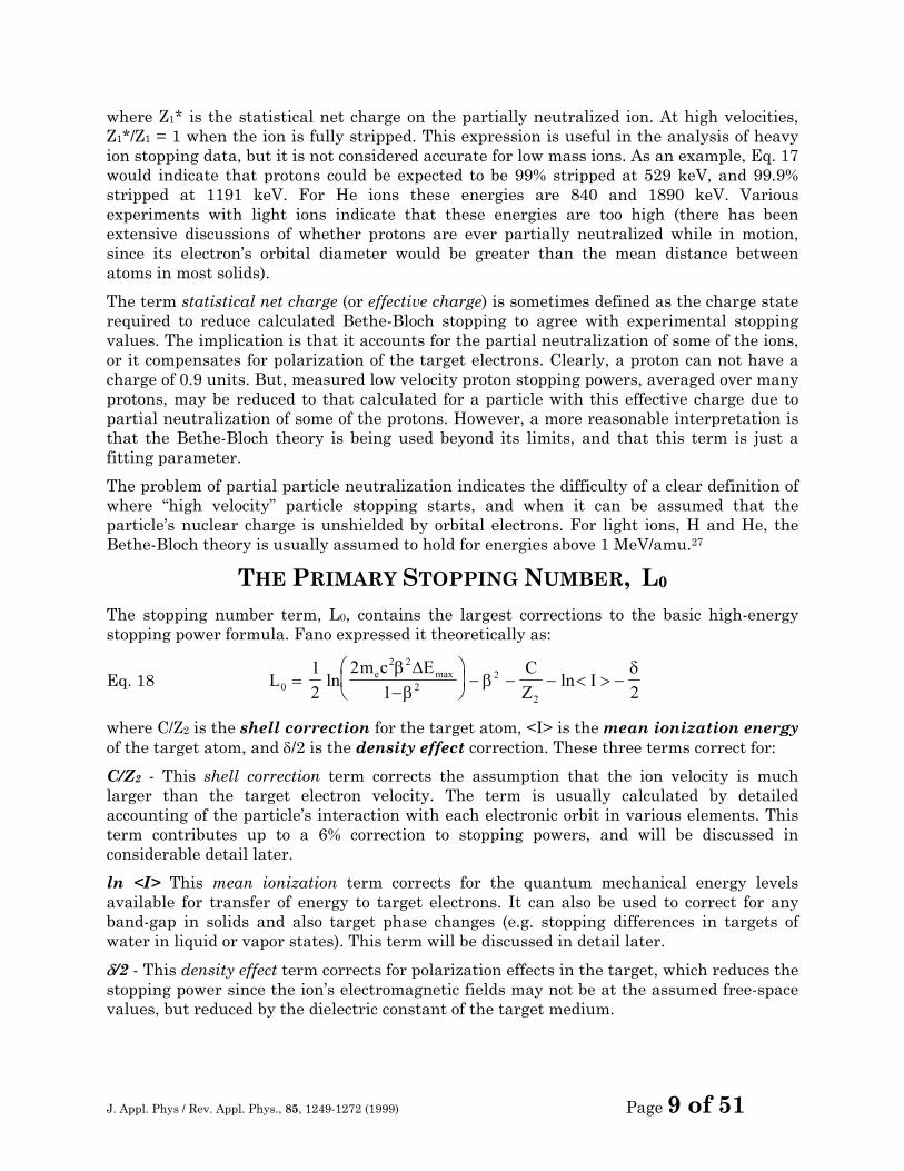
Figure 1 Evaluation of the term, ∆Emax, on Stopping Powers
The traditional derivation of the first stopping number term, L0, includes a term which indicates the largest possible energy loss in a single collision with a free electron, Eq. 19. This plots shows the error introduced to calculated stopping powers by approximating this term with the simpler form, Eq. 20, ∆Emax = (2mec2β2/1-β2). The full term adds a stopping correction which is always below 0.1% in effect, and usually is about 0.01%, which is far greater accuracy than other terms. So we shall use the abbreviated approximate form for ∆Emax hereafter.The term ∆Emax, in Eq. 18, is the largest possible energy loss in a single collision, and can be defined as:27
Eq. 19 ∆Em c m
MmM
e e emax /( )
=−
+
−+
−2
11
21
2 2
21
2 1 21
2 1β
β β
The magnitude the right-hand correction term to ∆Emax is quite small, and it is usually set to unity. In is shown the effect on calculated stopping powers by considering the full term, Eq. 19, and using on the abbreviated term,
Eq. 20 ∆Em ce
max ≈ −
21
2 2
2
ββ
The full term, Eq. 19, adds a correction which is always below 0.1%, and usually is contributes about 0.01%, which is beyond the accuracy of other corrective terms. So we shall use the abbreviated form for ∆Emax.
Note that for non-relativistic energies,
Eq. 21 ∆Em c
m veemax ≈ −
≈
21
22 2
22β
β
J. Appl. Phys / Rev. Appl. Phys., 85, 1249-1272 (1999) Page 11 of 51
The term ∆Emin is also sometimes used to restrict energy loss processes, which might occur with band-gap materials or insulators. Eq. 19 may be considered as the theoretical form of L0, since the term ∆Emin is derived by considerations of the target medium.
By substituting Eq. 21 into Eq. 18, the stopping number term, L0, is converted to an equivalent form that is widely used for the analysis of experimental data:
Eq. 22 Lm c C
ZIe
0
2 2
22
2
21 2
=−
− − − < > −ln ln
ββ
βδ
which is commonly simplified with the definition:
Eq. 11 f(β) ≡ ln [ 2mc2 β2 / (1-β2)]-β2
to obtain:
Eq. 23 L fCZ
I02 2
= − − < > −( ) lnβδ
With this equation, and using the Bethe-Bloch equation, Eq. 13, experimental data may be directly compared to theoretical evaluations of L0.
Shell Corrections, C/Z2
Shell corrections constitute a large correction to proton stopping powers in the energy range of 1-100 MeV, with a maximum correction of about 6%. It corrects the Bethe-Bloch theory requirement that the particle’s velocity is far greater than the bound electron velocity. As a particle velocity decreases from relativistic energies, the particle-electron collisions need to be considered with detailed evaluation of each target electron’s orbital bonding in order to obtain accurate stopping powers.
Shell corrections have been calculated using various approximations. As we shall show, these all produce approximately the same curves and are effective in correcting stopping powers.
The two most common approaches to calculate non-relativistic shell corrections are:
Hydrogenic Wave Functions - This HWF approach considers the particle interacting with individual target atom electrons which are described by hydrogenic wave functions.
Local Density Approximation - This LDA approach considers a particle interacting with a free electron gas (FEG) of various densities. The shell correction is then extracted by considering the target to be a linear superposition of FEG corrections based on their weighted densities in the target.
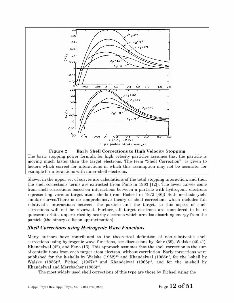
An early example of the results of these approaches is shown in
J. Appl. Phys / Rev. Appl. Phys., 85, 1249-1272 (1999) Page 12 of 51
Figure 2 Early Shell Corrections to High Velocity Stopping The basic stopping power formula for high velocity particles assumes that the particle is moving much faster than the target electrons. The term “Shell Correction” is given to factors which correct for interactions in which this assumption may not be accurate, for example for interactions with inner-shell electrons.
Shown in the upper set of curves are calculations of the total stopping interaction, and then the shell corrections terms are extracted (from Fano in 1963 [12]). The lower curves come from shell corrections based on interactions between a particle with hydrogenic electrons representing various target atom shells (from Bichsel in 1972 [46]) Both methods yield similar curves.There is no comprehensive theory of shell corrections which includes full relativistic interactions between the particle and the target, so this aspect of shell corrections will not be reviewed. Further, all target electrons are considered to be in quiescent orbits, unperturbed by nearby electrons which are also absorbing energy from the particle (the binary collision approximation).
Shell Corrections using Hydrogenic Wave Functions Many authors have contributed to the theoretical definition of non-relativistic shell corrections using hydrogenic wave functions, see discussions by Bohr (39), Walske (40,41), Khandelwal (42), and Fano (16). This approach assumes that the shell correction is the sum of contributions from each target atom electron, without correlation. Early corrections were published for the k-shells by Walske (1952)40 and Khandelwal (1968)42, for the l-shell by Walske (1956)41, Bichsel (1967)43 and Khandelwal (1968)42, and for the m-shell by Khandelwal and Merzbacher (1966)44.
The most widely used shell corrections of this type are those by Bichsel using the
J. Appl. Phys / Rev. Appl. Phys., 85, 1249-1272 (1999) Page 13 of 51
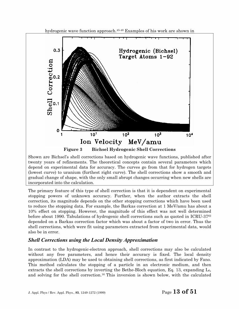
hydrogenic wave function approach.45-48 Examples of his work are shown in
Figure 3 Bichsel Hydrogenic Shell Corrections
Shown are Bichsel’s shell corrections based on hydrogenic wave functions, published after twenty years of refinements. The theoretical concepts contain several parameters which depend on experimental data for accuracy. The curves go from that for hydrogen targets (lowest curve) to uranium (furthest right curve). The shell corrections show a smooth and gradual change of shape, with the only small abrupt changes occurring when new shells are incorporated into the calculation.
The primary feature of this type of shell correction is that it is dependent on experimental stopping powers of unknown accuracy. Further, when the author extracts the shell correction, its magnitude depends on the other stopping corrections which have been used to reduce the stopping data. For example, the Barkas correction at 1 MeV/amu has about a 10% effect on stopping. However, the magnitude of this effect was not well determined before about 1990. Tabulations of hydrogenic shell corrections such as quoted in ICRU-3762 depended on a Barkas correction factor which was about a factor of two in error. Thus the shell corrections, which were fit using parameters extracted from experimental data, would also be in error.
Shell Corrections using the Local Density Approximation In contrast to the hydrogenic-electron approach, shell corrections may also be calculated without any free parameters, and hence their accuracy is fixed. The local density approximation (LDA) may be used to obtaining shell corrections, as first indicated by Fano. This method calculates the stopping of a particle in an electronic medium, and then extracts the shell corrections by inverting the Bethe-Bloch equation, Eq. 13, expanding L0, and solving for the shell correction.16 This inversion is shown below, with the calculated
J. Appl. Phys / Rev. Appl. Phys., 85, 1249-1272 (1999) Page 14 of 51
stopping of the particle indicated by the term, Scalc (to distinguish it from Sexp which will be used later):.
Eq. 24 22
111212
2
2 2ln)( LZLZ
ZZSIf
ZC calc ++−−><−=
δκββ
Examples of obtaining shell corrections using this method requires the calculation of stopping powers, S, using a different method, and then using Eq. 24 to extract shell corrections. Since calculations of stopping powers using the local density approximation does not use explicit shell corrections, the use of Eq. 24 allows these values to be directly compared to those calculated using hydrogenic wave functions.
The first attempt to evaluate electronic stopping cross-sections for protons in solids using the Lindhard stopping formalism and the local density approximation was by Bonderup who used Lenz-Jensen atoms to represent the atoms in the solid.89 This work was extended to isolated Hartree-Fock atoms by Rousseau et al.49 and to actual solid-state charge distributions by Ziegler.26
The LDA approach assumes that the gradient of electron densities in the target is small, and that the response of any volume element of the target is independent of other elements. The first assumption can be made tractable by using very small volume elements, but any error introduced by the second assumption is difficult to evaluate. Note that the LDA approach can not directly evaluate the effects of many basic solid state parameters such as band gaps and surfaces
Note that Eq. 24 requires the knowledge of the mean ionization potential, <I>. The theoretical calculation of the mean ionization potential has a long history, for it is a straight-forward calculation which may be done with almost any theoretical atom. Bonderup used the estimate that <I> = 11.4 Z2 (eV), and then solved for the shell correction term, C/Z2.
There have been many other calculations of <I>. Summaries of these calculations may be found in reviews such as by Fano22, Ziegler50, Ahlen21 or the ICRU27. In the local density approximation, the value of <I> may be calculated using : 51,88,89,52
Eq. 25 ln ln( )< > = ∫IZ
dVV1
20χ ω ρh
Where Z2 is the target atom atomic number, ω0 is the classical plasma frequency, ω0 = (4 π ρ e2 / m)½, and χ is a constant of the order of 1 and has been estimated by various theorists to be between 1 and 1.5.
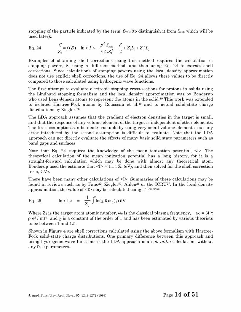
Shown in Figure 4 are shell corrections calculated using the above formalism with Hartree-Fock solid-state charge distributions. One primary difference between this approach and using hydrogenic wave functions is the LDA approach is an ab initio calculation, without any free parameters.
J. Appl. Phys / Rev. Appl. Phys., 85, 1249-1272 (1999) Page 15 of 51
Figure 4 Lindhard Winther LDA Shell Corrections
Shown are shell corrections by Ziegler, based on Lindhard Winther’s theory of particle stopping in a free electron gas, with the local density approximation (LDA) being used to generate shell corrections. This calculation is ab initio, without free parameters The curves go from that for hydrogen targets (lowest curve) to uranium (highest curve). The shell corrections show a smooth and gradual change of shape, with the only small abrupt changes occurring when new shells are incorporated into the calculation. Although this calculation is based on totally different assumptions as those based hydrogenic atoms, the results are quite similar.
Empirical Summed Shell and Ionization Corrections
Fano suggested22
that the calculation of the mean ionization potential, and the shell correction, could properly be linked as a single term which could be evaluated directly from experimental stopping data, Sexp, by rearranging Eq. 24:
Eq. 26 ln ( ) exp< > + = −
− + +I
CZ
fS
Z ZZ L Z L
2
2
2 12 1 1 1
222
ββ
κδ
where Sexp is the experimentally measured electronic stopping power. This approach has the advantage of isolating the two factors in the Bethe-Bloch equation which require extensive theoretical models, i.e. the mean ionization potential, <I>, and the shell correction, C/Z2. Using this equation, experimental data may be shown in reduced form and compared to theoretical calculations.
The importance of this approach is for the interpolation of stopping powers to targets with little experimental data. If the summed terms could be directly obtained from experimental data, then these can be used to interpolate for stopping powers of similar targets without
J. Appl. Phys / Rev. Appl. Phys., 85, 1249-1272 (1999) Page 16 of 51
experimental data. This technique was first used by Ziegler to extract the summed correction terms in order to normalize stopping calculations for targets without data, or to extrapolate to energies without experimental data.50
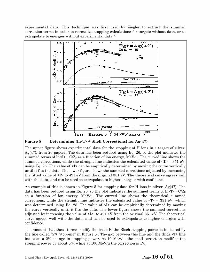
Figure 5 Determining (ln<I> + Shell Corrections) for Ag(47)
The upper figure shows experimental data for the stopping of H ions in a target of silver, Ag(47), from 26 papers. The data has been reduced using Eq. 26, so the plot indicates the summed terms of ln<I> +C/Z2 as a function of ion energy, MeV/u. The curved line shows the summed corrections, while the straight line indicates the calculated value of <I> = 351 eV, using Eq. 25. The value of <I> can be empirically determined by moving the curve vertically until it fits the data. The lower figure shows the summed corrections adjusted by increasing the fitted value of <I> to 491 eV from the original 351 eV. The theoretical curve agrees well with the data, and can be used to extrapolate to higher energies with confidence.
An example of this is shown in Figure 5 for stopping data for H ions in silver, Ag(47). The data has been reduced using Eq. 26, so the plot indicates the summed terms of ln<I> +C/Z2 as a function of ion energy, MeV/u. The curved line shows the theoretical summed corrections, while the straight line indicates the calculated value of <I> = 351 eV, which was determined using Eq. 25. The value of <I> can be empirically determined by moving the curve vertically until it fits the data. The lower figure shows the summed corrections adjusted by increasing the value of <I> to 491 eV from the original 351 eV. The theoretical curve agrees well with the data, and can be used to extrapolate to higher energies with confidence.
The amount that these terms modify the basic Bethe-Bloch stopping power is indicated by the line called “2% Stopping” in Figure 5 . The gap between this line and the thick <I> line indicates a 2% change in stopping power. At 10 MeV/u, the shell correction modifies the stopping power by about 6%, while at 100 MeV/u the correction is 1%.
J. Appl. Phys / Rev. Appl. Phys., 85, 1249-1272 (1999) Page 17 of 51
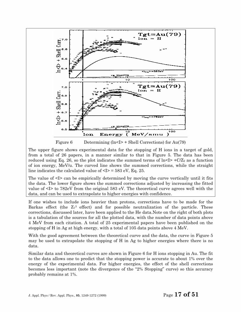
Figure 6 Determining (ln<I> + Shell Corrections) for Au(79)
The upper figure shows experimental data for the stopping of H ions in a target of gold, from a total of 26 papers, in a manner similar to that in Figure 5. The data has been reduced using Eq. 26, so the plot indicates the summed terms of ln<I> +C/Z2 as a function of ion energy, MeV/u. The curved line shows the summed corrections, while the straight line indicates the calculated value of <I> = 583 eV, Eq. 25.
The value of <I> can be empirically determined by moving the curve vertically until it fits the data. The lower figure shows the summed corrections adjusted by increasing the fitted value of <I> to 782eV from the original 583 eV. The theoretical curve agrees well with the data, and can be used to extrapolate to higher energies with confidence.
If one wishes to include ions heavier than protons, corrections have to be made for the Barkas effect (the Z13 effect) and for possible neutralization of the particle. These corrections, discussed later, have been applied to the He data.Note on the right of both plots is a tabulation of the sources for all the plotted data, with the number of data points above 4 MeV from each citation. A total of 25 experimental papers have been published on the stopping of H in Ag at high energy, with a total of 105 data points above 4 MeV.
With the good agreement between the theoretical curve and the data, the curve in Figure 5 may be used to extrapolate the stopping of H in Ag to higher energies where there is no data.
Similar data and theoretical curves are shown in Figure 6 for H ions stopping in Au. The fit to the data allows one to predict that the stopping power is accurate to about 1% over the energy of the experimental data. For higher energies, the effect of the shell corrections becomes less important (note the divergence of the “2% Stopping” curve) so this accuracy probably remains at 1%.
J. Appl. Phys / Rev. Appl. Phys., 85, 1249-1272 (1999) Page 18 of 51
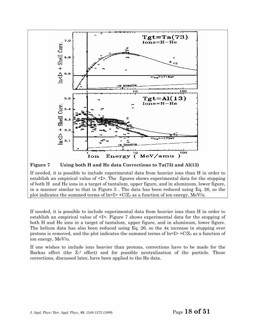
Figure 7 Using both H and He data Corrections to Ta(73) and Al(13)
If needed, it is possible to include experimental data from heavier ions than H in order to establish an empirical value of <I>. The figures shows experimental data for the stopping of both H and He ions in a target of tantalum, upper figure, and in aluminum, lower figure, in a manner similar to that in Figure 5 . The data has been reduced using Eq. 26, so the plot indicates the summed terms of ln<I> +C/Z2 as a function of ion energy, MeV/u.
If needed, it is possible to include experimental data from heavier ions than H in order to establish an empirical value of <I>. Figure 7 shows experimental data for the stopping of both H and He ions in a target of tantalum, upper figure, and in aluminum, lower figure. The helium data has also been reduced using Eq. 26, so the 4x increase in stopping over protons is removed, and the plot indicates the summed terms of ln<I> +C/Z2 as a function of ion energy, MeV/u.
If one wishes to include ions heavier than protons, corrections have to be made for the Barkas effect (the Z13 effect) and for possible neutralization of the particle. These corrections, discussed later, have been applied to the He data.
J. Appl. Phys / Rev. Appl. Phys., 85, 1249-1272 (1999) Page 19 of 51
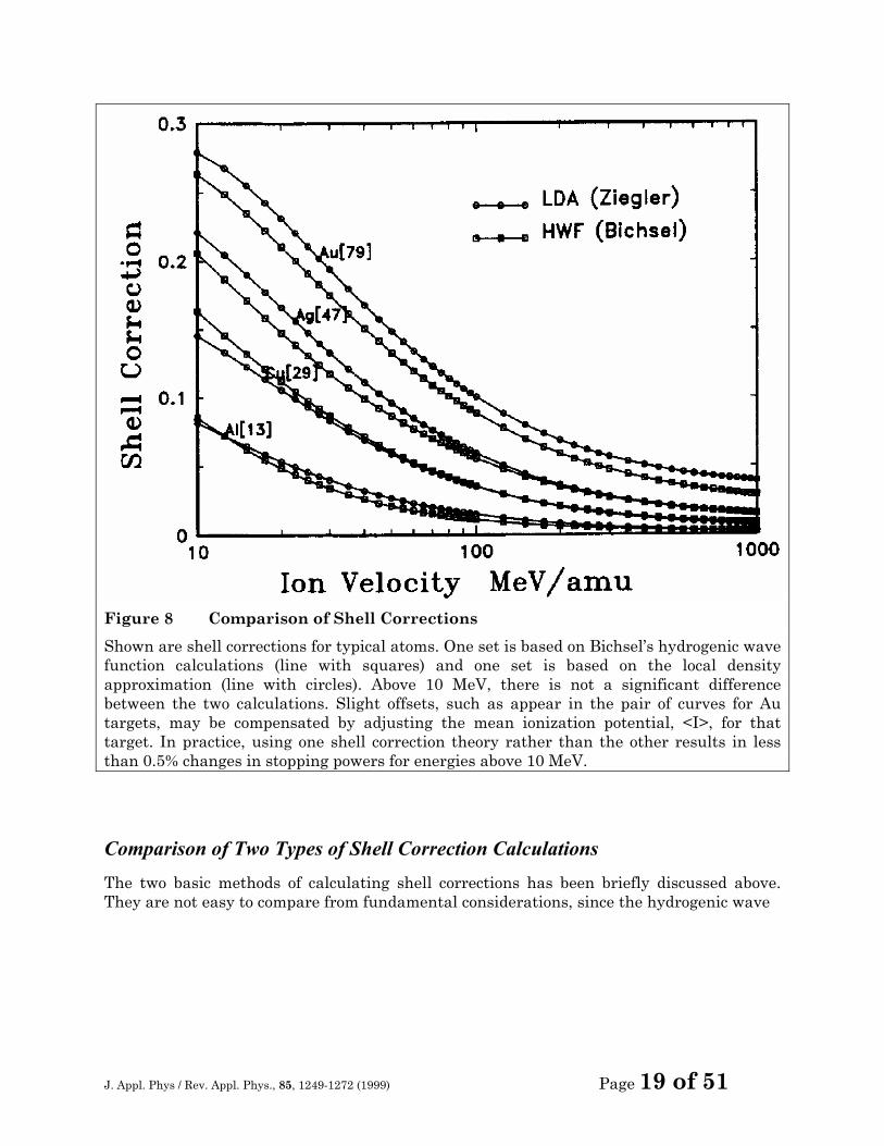
Figure 8 Comparison of Shell Corrections
Shown are shell corrections for typical atoms. One set is based on Bichsel’s hydrogenic wave function calculations (line with squares) and one set is based on the local density approximation (line with circles). Above 10 MeV, there is not a significant difference between the two calculations. Slight offsets, such as appear in the pair of curves for Au targets, may be compensated by adjusting the mean ionization potential, <I>, for that target. In practice, using one shell correction theory rather than the other results in less than 0.5% changes in stopping powers for energies above 10 MeV.
Comparison of Two Types of Shell Correction Calculations The two basic methods of calculating shell corrections has been briefly discussed above. They are not easy to compare from fundamental considerations, since the hydrogenic wave
J. Appl. Phys / Rev. Appl. Phys., 85, 1249-1272 (1999) Page 20 of 51
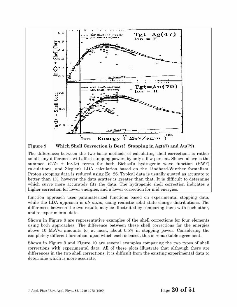
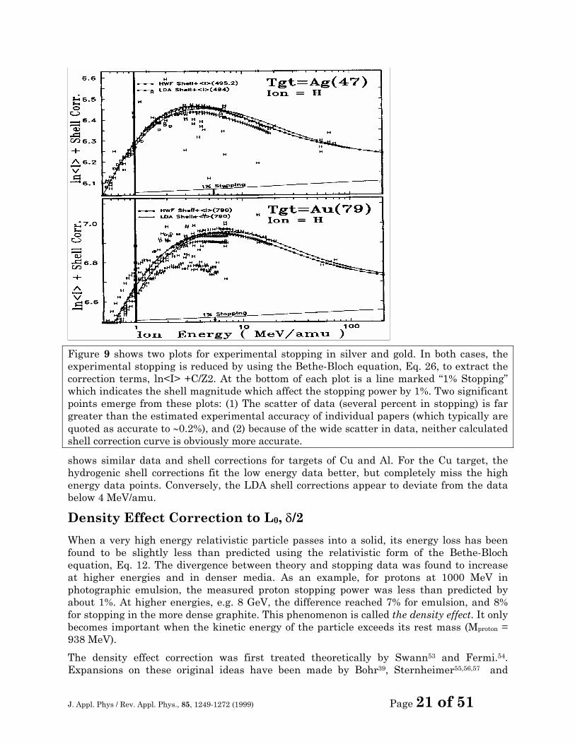
Figure 9 Which Shell Correction is Best? Stopping in Ag(47) and Au(79)
The differences between the two basic methods of calculating shell corrections is rather small- any differences will affect stopping powers by only a few percent. Shown above is the summed (C/Z2 + ln<I>) terms for both Bichsel’s hydrogenic wave function (HWF) calculations, and Ziegler’s LDA calculation based on the Lindhard-Winther formalism. Proton stopping data is reduced using Eq. 26. Typical data is usually quoted as accurate to better than 1%, however the data scatter is greater than that. It is difficult to determine which curve more accurately fits the data. The hydrogenic shell correction indicates a higher correction for lower energies, and a lower correction for mid energies.
function approach uses paramaterized functions based on experimental stopping data, while the LDA approach is ab initio, using realistic solid state charge distributions. The differences between the two results may be illustrated by comparing them with each other, and to experimental data.
Shown in Figure 8 are representative examples of the shell corrections for four elements using both approaches. The difference between these shell corrections for the energies above 10 MeV/u amounts to, at most, about 0.5% in stopping power. Considering the completely different formalism upon which each is based, this is remarkable agreement.
Shown in Figure 9 and Figure 10 are several examples comparing the two types of shell corrections with experimental data. All of these plots illustrate that although there are differences in the two shell corrections, it is difficult from the existing experimental data to determine which is more accurate.
J. Appl. Phys / Rev. Appl. Phys., 85, 1249-1272 (1999) Page 21 of 51
Figure 9 shows two plots for experimental stopping in silver and gold. In both cases, the experimental stopping is reduced by using the Bethe-Bloch equation, Eq. 26, to extract the correction terms, ln<I> +C/Z2. At the bottom of each plot is a line marked “1% Stopping” which indicates the shell magnitude which affect the stopping power by 1%. Two significant points emerge from these plots: (1) The scatter of data (several percent in stopping) is far greater than the estimated experimental accuracy of individual papers (which typically are quoted as accurate to ∼0.2%), and (2) because of the wide scatter in data, neither calculated shell correction curve is obviously more accurate.
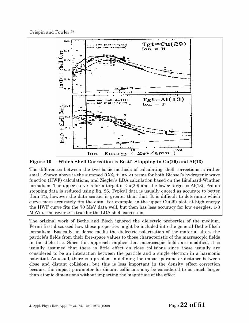
shows similar data and shell corrections for targets of Cu and Al. For the Cu target, the hydrogenic shell corrections fit the low energy data better, but completely miss the high energy data points. Conversely, the LDA shell corrections appear to deviate from the data below 4 MeV/amu.
Density Effect Correction to L0, δ/2
When a very high energy relativistic particle passes into a solid, its energy loss has been found to be slightly less than predicted using the relativistic form of the Bethe-Bloch equation, Eq. 12. The divergence between theory and stopping data was found to increase at higher energies and in denser media. As an example, for protons at 1000 MeV in photographic emulsion, the measured proton stopping power was less than predicted by about 1%. At higher energies, e.g. 8 GeV, the difference reached 7% for emulsion, and 8% for stopping in the more dense graphite. This phenomenon is called the density effect. It only becomes important when the kinetic energy of the particle exceeds its rest mass (Mproton = 938 MeV).
The density effect correction was first treated theoretically by Swann53 and Fermi.54. Expansions on these original ideas have been made by Bohr39, Sternheimer55,56,57 and
J. Appl. Phys / Rev. Appl. Phys., 85, 1249-1272 (1999) Page 22 of 51
Crispin and Fowler.58
Figure 10 Which Shell Correction is Best? Stopping in Cu(29) and Al(13)
The differences between the two basic methods of calculating shell corrections is rather small. Shown above is the summed (C/Z2 + ln<I>) terms for both Bichsel’s hydrogenic wave function (HWF) calculations, and Ziegler’s LDA calculation based on the Lindhard-Winther formalism. The upper curve is for a target of Cu(29) and the lower target is Al(13). Proton stopping data is reduced using Eq. 26. Typical data is usually quoted as accurate to better than 1%, however the data scatter is greater than that. It is difficult to determine which curve more accurately fits the data. For example, in the upper Cu(29) plot, at high energy the HWF curve fits the 70 MeV data well, but then has less accuracy for low energies, 1-3 MeV/u. The reverse is true for the LDA shell correction.
The original work of Bethe and Bloch ignored the dielectric properties of the medium. Fermi first discussed how these properties might be included into the general Bethe-Bloch formalism. Basically, in dense media the dielectric polarization of the material alters the particle’s fields from their free-space values to those characteristic of the macroscopic fields in the dielectric. Since this approach implies that macroscopic fields are modified, it is usually assumed that there is little effect on close collisions since these usually are considered to be an interaction between the particle and a single electron in a harmonic potential. As usual, there is a problem in defining the impact parameter distance between close and distant collisions, but this is less important in the density effect correction because the impact parameter for distant collisions may be considered to be much larger than atomic dimensions without impacting the magnitude of the effect.
J. Appl. Phys / Rev. Appl. Phys., 85, 1249-1272 (1999) Page 23 of 51
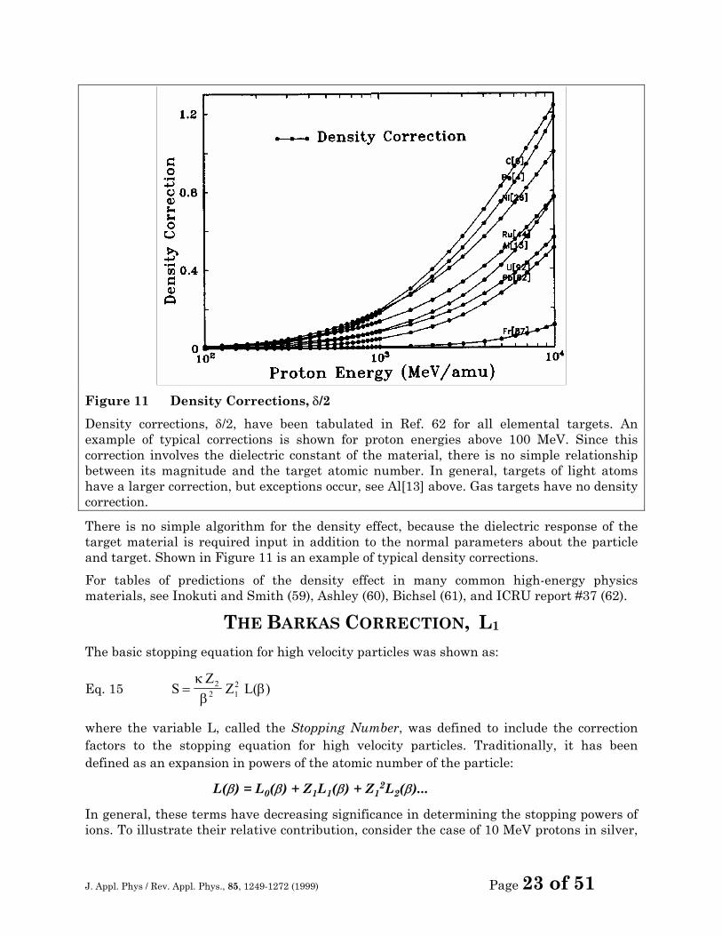
Figure 11 Density Corrections, δ/2
Density corrections, δ/2, have been tabulated in Ref. 62 for all elemental targets. An example of typical corrections is shown for proton energies above 100 MeV. Since this correction involves the dielectric constant of the material, there is no simple relationship between its magnitude and the target atomic number. In general, targets of light atoms have a larger correction, but exceptions occur, see Al[13] above. Gas targets have no density correction.
There is no simple algorithm for the density effect, because the dielectric response of the target material is required input in addition to the normal parameters about the particle and target. Shown in Figure 11 is an example of typical density corrections.
For tables of predictions of the density effect in many common high-energy physics materials, see Inokuti and Smith (59), Ashley (60), Bichsel (61), and ICRU report #37 (62).
THE BARKAS CORRECTION, L1 The basic stopping equation for high velocity particles was shown as:
Eq. 15 SZ
Z L=κβ
β22 1
2 ( )
where the variable L, called the Stopping Number, was defined to include the correction factors to the stopping equation for high velocity particles. Traditionally, it has been defined as an expansion in powers of the atomic number of the particle:
L(β) = L0(β) + Z1L1(β) + Z12L2(β)...
In general, these terms have decreasing significance in determining the stopping powers of ions. To illustrate their relative contribution, consider the case of 10 MeV protons in silver,
J. Appl. Phys / Rev. Appl. Phys., 85, 1249-1272 (1999) Page 24 of 51
Ag(47) - the terms will contribute: L0 ≈ 98.8%, Z1L1 ≈ 1.1%, Z12L2 ≈ 0.1%. However, there are special situations in which the higher-order terms become more significant.
Much of the work on the higher order terms, L1 and L2, has been stimulated by two remarkable kinds of experimental evidence which highlighted inadequacies in the Bethe-Bloch equation:
1. The discovery of different ranges for particles at the same velocity and in the same target, whose only difference was that one had a positive charge and the other had a negative charge. Since the Bethe-Bloch equation, Eq. 15 above, shows only a stopping dependence on Z12, there should be no difference in the stopping power of positive particles when compared to those of equivalent negative particles.
2. The discovery of errors in the scaling of stopping powers for particles at the same velocity and in the same target, whose only difference was their amount of charge. According to the Bethe-Bloch equation, Eq. 15, a particle with charge +2 should have four times the stopping of a similar particle with charge +1. However, the stopping of +2 charged particles was discovered to exceed 4x that of an equivalent +1 charged particle
Both of these experimental results will be discussed below, with some emphasis on the historical path leading to an understanding of how these remarkably different experiments led to a single explanation and solution. This final resolution concerns a correction to the basic Bethe-Bloch assumption that the initial distribution of target electrons are uniformly distributed about quiescent atoms. However, a positive charge will pull these target electrons towards it as it approaches, increasing the local electron density, while a negative charge will repel them. For the case of similar negative and positive particles, example (1) above , this polarization of the target will cause positive particles to pass through a slightly higher density of target electrons, increasing its energy loss relative to that of a negatively charged particle. At high velocities this effect may becomes negligible, since the target electrons do not have time to move, but near the maximum of the energy loss of light particles, about 1 MeV/amu, this effect becomes apparent. In the case of particles with different charges, example (2) above, a higher charged particle will pass through a slightly higher density of target electrons compared to the singly charged particle, increasing its stopping above what might be expected.
The Barkas Effect from Charge Sign Considerations
The Barkas Correction, Z1L1, was named after Walter Barkas, who discovered in 1956 a difference in the ranges of positive and negative pions in photographic emulsion, and showed that the range of negative pions was longer than that of positive pions.63 This range difference was small, about 0.36%, but Barkas measured it with great precision and established the clear unexpected difference. The explanation of this difference was later suggested by Barkas as being caused by a correction to the first-order Born approximation of the Bethe-Bloch equation.64 Positive projectiles tend to pull electrons towards its trajectory, while negative particles tend to repel them. The early experimental work by Barkas and others has been reviewed by Heckman.65
This work prompted a series of papers by Ashley et al. from 1972-74.66,67,68 These papers presented a non-relativistic stopping power correction based on a harmonic oscillator approach. The authors assumed that close collisions would not be significant in the L1 correction, and presented results for a correction to distant collision events. They assumed a target electron in a harmonic oscillator potential, which for small displacements varied
J. Appl. Phys / Rev. Appl. Phys., 85, 1249-1272 (1999) Page 25 of 51
the force on the electron. This was a correction to the original approach of Bohr who assumed that the force on the electron was independent of small displacements.6 The Ashley correction led to a term in Z13 for the energy transfer to distant collisions. They suggested for the high velocity limit a form:
Eq. 27
=
ωωωπ
av
vmeZLZ
7.1ln
23
3
21
11
where v is the velocity of the particle, ω is the free electron gas plasma frequency, and aω is lower limit of the impact parameter for the distant collisions. This high velocity limit is for v1 >> ωaω. The authors refined this approximation over several papers, and produced a useful paramaterized form:
Eq. 28 Z LZ F b x
Z xArb
1 11
1 2
21 2 3 2=
( / )/
/ /
where x = (β α)2 / Z2 and b = χηZ21/6
The term χ is a free-electron-gas parameter which corrects for binding forces, and has a value of about 21/2. This expression includes a tabulated function, Farb, included in the final paper.
Soon after Ashley’s first paper, Jackson and McCarthy suggested a different minimum impact parameter, aω = (h2mω)½.69 Hill and Merzbacher performed a similar quantal calculation, but expanded the electron’s harmonic potential to second order. 70
Lindhard reviewed these approaches, and suggested that the omission of close collisions from the above studies was wrong, and that these effects would be about as great as the distant collisions.71 The final correction would be almost twice what had been previously estimated. This suggestion of Lindhard was later supported by experiments measuring the stopping of p_ (anti-protons) in silicon.72
J. Appl. Phys / Rev. Appl. Phys., 85, 1249-1272 (1999) Page 26 of 51
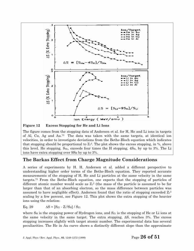
Figure 12 Excess Stopping for He and Li Ions
The figure comes from the stopping data of Andersen et al. for H, He and Li ions in targets of Al, Cu, Ag and Au.73 The data was taken with the same targets, at identical ion velocities, in order to investigate deviations from the Bethe-Bloch equation which indicates that stopping should be proportional to Z12. The plot shows the excess stopping, in %, above this level. He stopping, SHe, exceeds four times the H stopping, 4SH, by up to 3%. The Li ions have extra stopping over 9SH by up to 3%.
The Barkas Effect from Charge Magnitude Considerations
A series of experiments by H. H. Andersen et al. added a different perspective to understanding higher order terms of the Bethe-Bloch equation. They reported accurate measurements of the stopping of H, He and Li particles at the same velocity in the same targets.73 From the Bethe-Bloch equation, one expects that the stopping of particles of different atomic number would scale as Z12 (the mass of the particle is assumed to be far larger than that of an absorbing electron, so the mass difference between particles was assumed to have negligible effect). Andersen found that the ratio of stopping exceeded Z12 scaling by a few percent, see Figure 12. This plot shows the extra stopping of the heavier ions using the relation:
Eq. 29 ∆S = [SZ1 - Z12SH] / SZ1
where SH is the stopping power of Hydrogen ions, and SZ1 is the stopping of He or Li ions at the same velocity in the same target. The extra stopping, ∆S, reaches 3%. The excess stopping increases slightly with target atomic number. The experimental data has several peculiarities. The He in Au curve shows a distinctly different slope than the approximate
J. Appl. Phys / Rev. Appl. Phys., 85, 1249-1272 (1999) Page 27 of 51
1/E decrease of the other He stopping curves. One He curve (Ag target) and all the Li curves show a peak in the excess stopping, while the others show no peak.
Andersen et al. suggested that their experimental stopping powers for H, He and Li (covering the energy range of 0.8-7.2 MeV/u) could be fit by using complex Barkas + Bloch terms (the Bloch correction will be discussed in the next section):
Eq. 30 Z12L2 (Bloch term) = -1.6 ( Z1 v0 / v )2
Eq. 31 Z1L1 (Barkas term) = ( )
− V
VZZL ln264.0168.2
22/12
10
V ≡ ( v / v0Z21/3 )
where Z1 is the particle charge, v is the particle velocity and v0 is the Bohr velocity (25 keV/u) and Z2 is the target atomic number. Note that the Barkas term depends on L0, the basic stopping number which includes shell corrections and the mean ionization potential of the target. These proposed correction terms are not clean expansion terms relative to the particle’s charge, which was the original assumption in the expansion of the Bethe-Bloch equation into stopping numbers dependent on integer powers of the particle charge.
Bichsel approached the problem of the Barkas Correction by a limited empirical approach.27,48,83 He started with a variation of the Ashley equation, Eq. 27, and used only Andersen’s experimental stopping data shown in Figure 12 to extract a simpler Z1L1 correction expression than that shown in Eq. 30 and Eq. 31. His results were:
Eq. 32 Z1 L1 = Z C12/ β α
where C and α were constants which varied with various targets: Target C α Al (13) .001050 0.80
Cu (29) .002415 0.65 Ag (47) .006812 0.45 Au (79) .002833 0.60
This fit was limited to He ions over the narrow energy range of the experimental data, 1-6 MeV/u. The expression is asymptotically incorrect since it rapidly diverges for energies below 1 MeV/u.
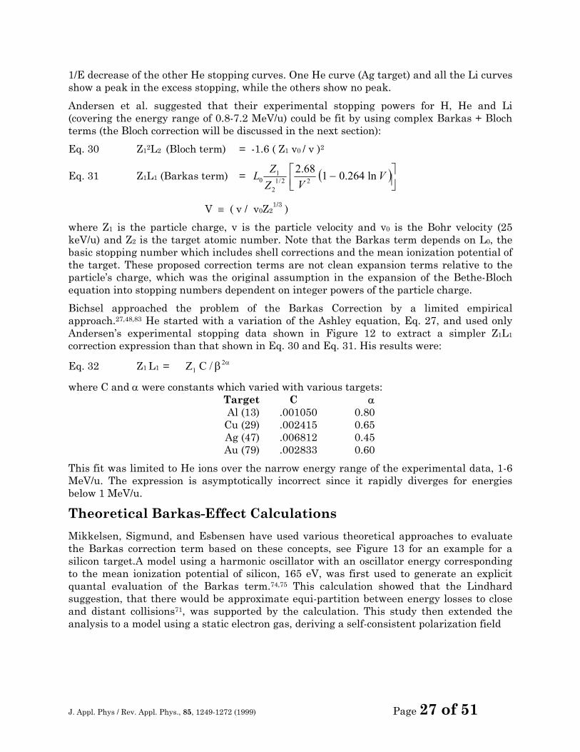
Theoretical Barkas-Effect Calculations
Mikkelsen, Sigmund, and Esbensen have used various theoretical approaches to evaluate the Barkas correction term based on these concepts, see Figure 13 for an example for a silicon target.A model using a harmonic oscillator with an oscillator energy corresponding to the mean ionization potential of silicon, 165 eV, was first used to generate an explicit quantal evaluation of the Barkas term.74,75 This calculation showed that the Lindhard suggestion, that there would be approximate equi-partition between energy losses to close and distant collisions71, was supported by the calculation. This study then extended the analysis to a model using a static electron gas, deriving a self-consistent polarization field
J. Appl. Phys / Rev. Appl. Phys., 85, 1249-1272 (1999) Page 28 of 51
Figure 13 Theoretical evaluation of the Barkas Correction for Silicon
Shown are evaluations of the Barkas effect using various models by Sigmund, Mikkelsen and Esbensen.74-79 The single oscillator model considers the target as an oscillator with a resonance frequency of I/h, where I is the mean ionization energy or the target atoms. The oscillator model uses a spherical harmonic oscillator, with the Born series evaluated up to second order and preserving shell corrections in evaluating the Barkas correction. The Lindhard gas model assumes the Lindhard interaction of a particle to an electron gas with a resonance frequency of I/h.87 The dielectric model considers the particle in a self-consistent polarized dense electron gas, and uses the local density model to evaluate the Barkas correction.
for the medium, and again reached the conclusion that the Lindhard ideas were approximately correct.76 The evaluation of the Barkas correction term was also evaluated using the local-density-approximation (see Appendix) using a Lenz-Jensen model for the target atoms.77 This work was further extended to find a complete solution using a time-dependent Schrodinger equation for the interaction between the particle and a target electron represented as a quantum harmonic oscillator.78
All these approaches have been reviewed by Sigmund, who discussed many relevant approaches to stopping powers in the region where the Barkas correction was significant.79
Unified Barkas Correction Factor
The Barkas effect is caused by target electrons responding to the approaching particle, and slightly changing their orbits before any energy loss interaction occurs (called target polarization). At high energies (above 20 v0 ≈ 10 MeV/u) the Barkas effect becomes insignificant because the ion will be moving too fast to cause initial motion of the target electrons. At low energies, <<1 MeV/u, the Barkas effect is difficult to isolate in experiments because of the onset of neutralization of the ion. That is, at low velocities
J. Appl. Phys / Rev. Appl. Phys., 85, 1249-1272 (1999) Page 29 of 51
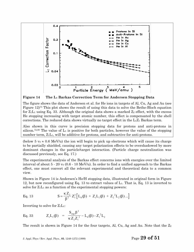
Figure 14 The L1 Barkas Correction Term for Andersen Stopping Data
The figure shows the data of Andersen et al. for He ions in targets of Al, Cu, Ag and Au (see Figure 12)73 This plot shows the result of using this data to solve the Bethe-Bloch equation for Z1L1 using Eq. 33. Although the original data shows a marked Z2 effect, with the excess He stopping increasing with target atomic number, this effect is compensated by the shell corrections. The reduced data shows virtually no target effect in the L1Z1 Barkas term.
Also shown in this curve is precision stopping data for protons and anti-protons in silicon.72,80 The value of L1 is positive for both particles, however the value of the stopping number term, Z1L1, will be additive for protons, and subtractive for anti-protons.
(below 5 v0 ≈ 0.6 MeV/u) the ion will begin to pick up electrons which will cause its charge to be partially shielded, causing any target polarization effects to be overshadowed by more dominant changes in the particle/target interaction. (Particle charge neutralization was discussed previously, see Eq. 17.)
The experimental analysis of the Barkas effect concerns ions with energies over the limited interval of about 5 - 20 v0 (0.6 - 10 MeV/u). In order to find a unified approach to the Barkas effect, one must convert all the relevant experimental and theoretical data to a common view.
Shown in Figure 14 is Andersen’s He/H stopping data, illustrated in original form in Figure 12, but now reconfigured using Eq. 13 to extract values of L1. That is, Eq. 13 is inverted to solve for Z1L1 as a function of the experimental stopping powers:
Eq. 13 [ ]SZ
Z L=κβ
β β β22 1
2 2L ( ) + Z L ( ) + Z ( ) ...0 1 1 2 2
Inverting to solve for Z1L1:
Eq. 33 Z L ( ) = ( ) -1 1 0ββ
κβ
SZ Z
L Z Lexp2
2 12 1
22−
The result is shown in Figure 14 for the four targets, Al, Cu, Ag and Au. Note that the Z2
J. Appl. Phys / Rev. Appl. Phys., 85, 1249-1272 (1999) Page 30 of 51
dependency noted in the original data has disappeared, since this has been accounted for by the L0 shell corrections.
Also shown in Figure 14 are representative stopping results from precision measurements of protons and anti-protons in silicon, discussed before.72,80 These papers extracted the Barkas correction directly by assuming it was proportional to exactly one-half the difference between proton and anti-proton stopping in the same target, at the same velocity. The Barkas factor was determined by dividing this stopping difference by the Bethe-Bloch pre-factor, shown above in Eq. 13. Remarkably, these results overlap the He results for four different targets, reinforcing the conclusion that the Barkas term is independent of target atomic number.
Most important, Figure 14 shows that the two basic Barkas effects described above are probably the same effect, seen in two different kinds of experiments. The proton/anti-proton stopping shows differences associated with the particle charge sign, while the He/H excess stopping shows differences from the basic Bethe-Bloch Z12 stopping formalism. Both of these effects are caused by target electrons having time to polarize (move) in response to the incident charged particle. For the anti-proton data, Z1 = -1, L1 will be positive as shown but the value of Z1L1 will be negative. Hence Z1L1 for protons will contribute to the stopping (increasing its magnitude) while it will be subtracted from the anti-proton stopping. This may be viewed as an increased local electron density for the positive particle, and a decreased local electron density for the negative anti-protons.
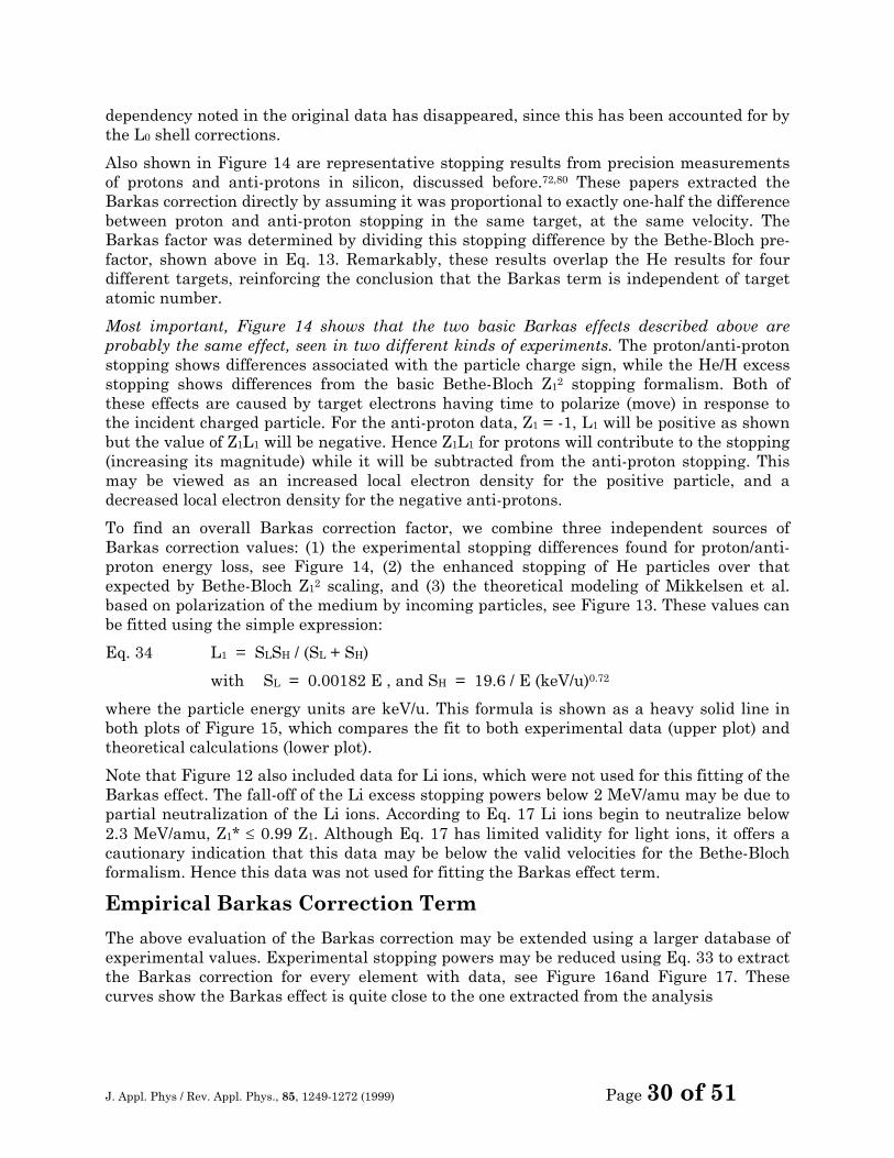
To find an overall Barkas correction factor, we combine three independent sources of Barkas correction values: (1) the experimental stopping differences found for proton/anti-proton energy loss, see Figure 14, (2) the enhanced stopping of He particles over that expected by Bethe-Bloch Z12 scaling, and (3) the theoretical modeling of Mikkelsen et al. based on polarization of the medium by incoming particles, see Figure 13. These values can be fitted using the simple expression:
Eq. 34 L1 = SLSH / (SL + SH)
with SL = 0.00182 E , and SH = 19.6 / E (keV/u)0.72
where the particle energy units are keV/u. This formula is shown as a heavy solid line in both plots of Figure 15, which compares the fit to both experimental data (upper plot) and theoretical calculations (lower plot).
Note that Figure 12 also included data for Li ions, which were not used for this fitting of the Barkas effect. The fall-off of the Li excess stopping powers below 2 MeV/amu may be due to partial neutralization of the Li ions. According to Eq. 17 Li ions begin to neutralize below 2.3 MeV/amu, Z1* ≤ 0.99 Z1. Although Eq. 17 has limited validity for light ions, it offers a cautionary indication that this data may be below the valid velocities for the Bethe-Bloch formalism. Hence this data was not used for fitting the Barkas effect term.
Empirical Barkas Correction Term
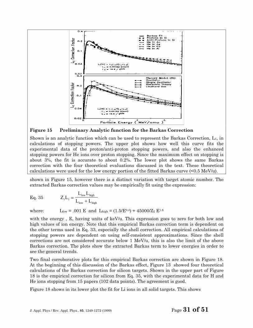
The above evaluation of the Barkas correction may be extended using a larger database of experimental values. Experimental stopping powers may be reduced using Eq. 33 to extract the Barkas correction for every element with data, see Figure 16and Figure 17. These curves show the Barkas effect is quite close to the one extracted from the analysis
J. Appl. Phys / Rev. Appl. Phys., 85, 1249-1272 (1999) Page 31 of 51
Figure 15 Preliminary Analytic function for the Barkas Correction
Shown is an analytic function which can be used to represent the Barkas Correction, L1, in calculations of stopping powers. The upper plot shows how well this curve fits the experimental data of the proton/anti-proton stopping powers, and also the enhanced stopping powers for He ions over proton stopping. Since the maximum effect on stopping is about 3%, the fit is accurate to about 0.2%. The lower plot shows the same Barkas correction with the four theoretical evaluations discussed in the text. These theoretical calculations were used for the low energy portion of the fitted Barkas curve (<0.5 MeV/u).
shown in Figure 15, however there is a distinct variation with target atomic number. The extracted Barkas correction values may be empirically fit using the expression:
Eq. 35 Z LL L
L Llow high
low high1 1 = +
where: Llow = .001 E and Lhigh = (1.5/E0.4) + 45000/Z2 E1.6
with the energy , E, having units of keV/u. This expression goes to zero for both low and high values of ion energy. Note that this empirical Barkas correction term is dependent on the other terms used in Eq. 33, especially the shell correction. All empirical calculations of stopping powers are dependent on using self-consistent approximations. Since the shell corrections are not considered accurate below 1 MeV/u, this is also the limit of the above Barkas correction. The plots show the extracted Barkas term to lower energies in order to see the general trends.
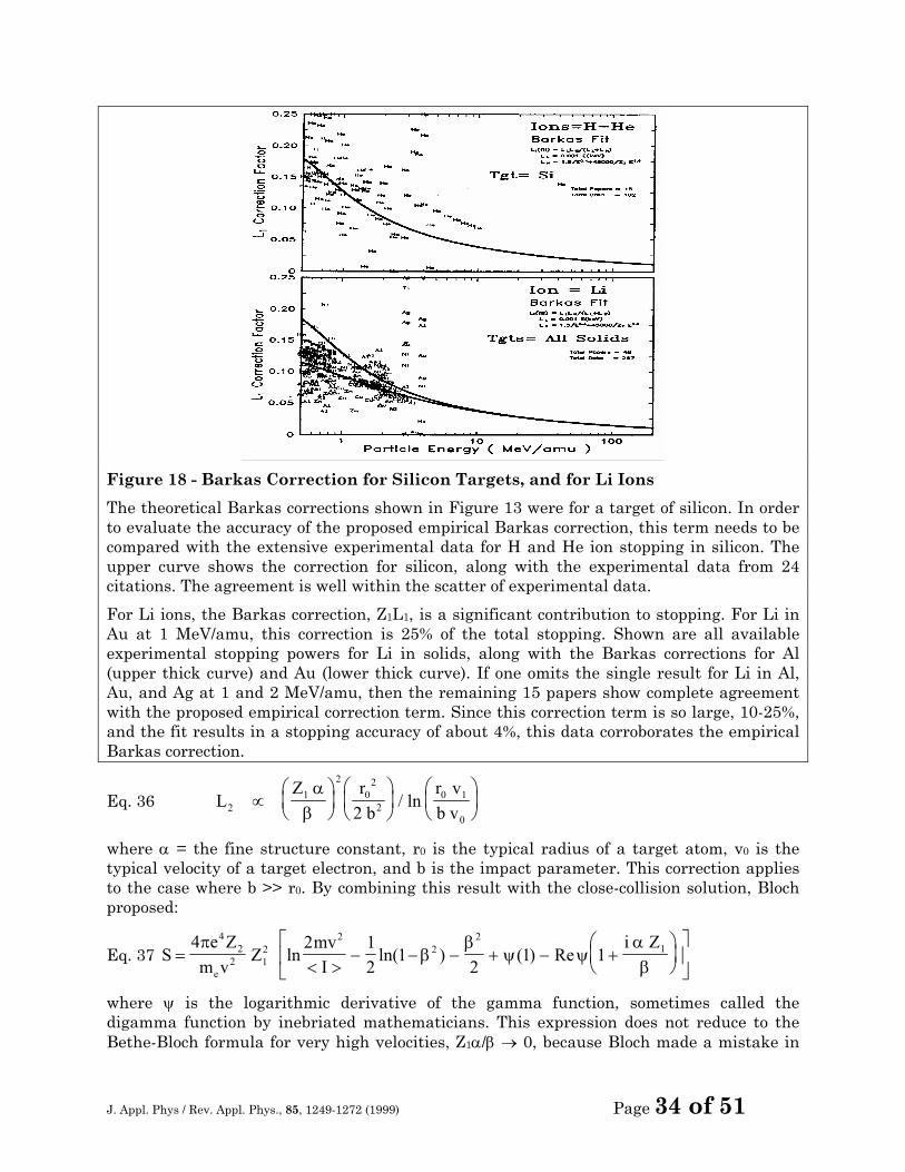
Two final corroborative plots for this empirical Barkas correction are shown in Figure 18. At the beginning of this discussion of the Barkas effect, Figure 13 showed four theoretical calculations of the Barkas correction for silicon targets. Shown in the upper part of Figure 18 is the empirical correction for silicon from Eq. 35, with the experimental data for H and He ions stopping from 15 papers (102 data points). The agreement is good.
Figure 18 shows in its lower plot the fit for Li ions in all solid targets. This shows
J. Appl. Phys / Rev. Appl. Phys., 85, 1249-1272 (1999) Page 32 of 51
Figure 16 Barkas Correction for C, Al, Fe, Co, Ni and Cu
Shown are the Barkas correction terms to the Bethe-Bloch stopping equation extracted from experimental data using Eq. 33. The upper curve shows data from C and Al targets, while the bottom curve shows data from Fe, Co, Ni and Cu targets. Clearly, the data do not indicate a target-independent Barkas correction value in the two plots. An empirical Barkas correction expression, Eq. 35, is shown as a thick line in each plot. In the upper plot, for C and Al targets, the two lines are clearly separate, with the upper curve being for carbon targets. In the lower plot, the separate curves for the Barkas correction for Fe, Co, Ni and Cu are too close to separate. Note that this empirical Barkas correction is only valid when used with the other corrections used in Eq. 33, especially the shell correction term.
important support for this Barkas correction, Z1L1, because of its very large contribution to the stopping of Li ions. For example, for 1 MeV/amu Li ions in Au, the Barkas correction is 25% of the total stopping power. However, the scatter of data in the figure is quite small, such that the average stopping error is less than 4.
THE BLOCH CORRECTION, L2 The basic stopping equation for high velocity particles, as traditionally formulated, was shown as:
Eq. 15 SZ
Z L=κβ
β22 1
2 ( )
where the variable L, called the Stopping Number, was defined to include the correction factors to the stopping equation for high velocity particles. Traditionally, it is defined as
J. Appl. Phys / Rev. Appl. Phys., 85, 1249-1272 (1999) Page 33 of 51
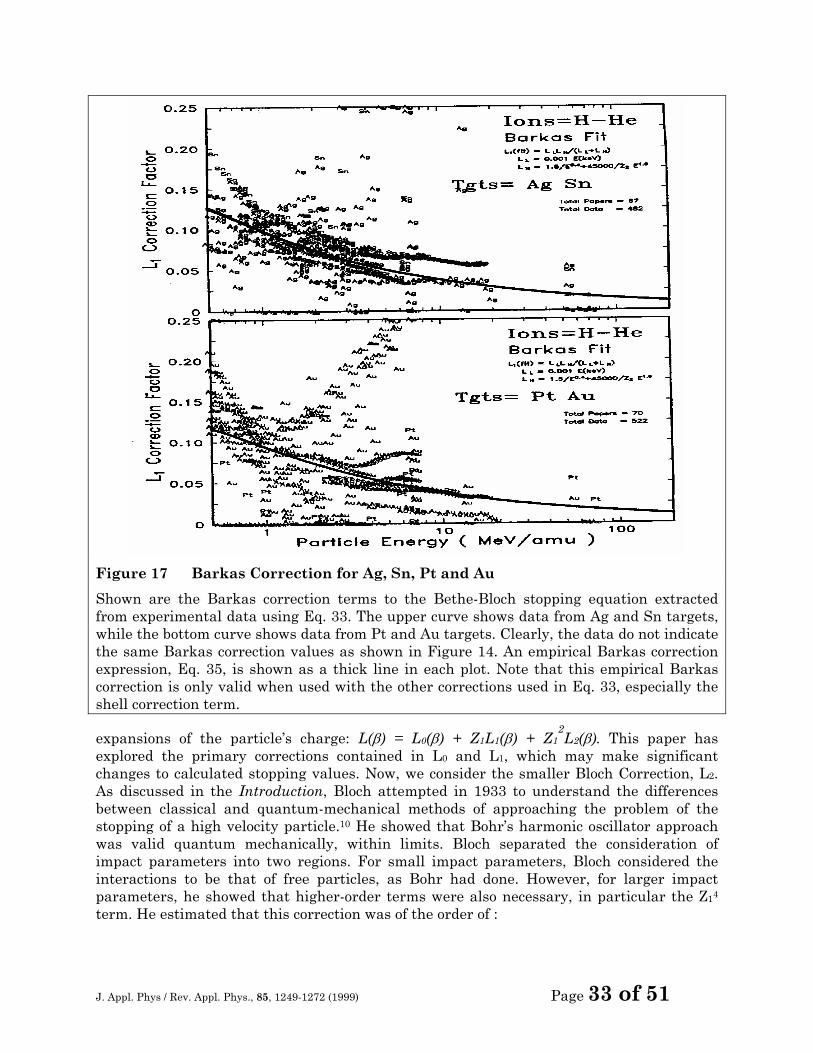
Figure 17 Barkas Correction for Ag, Sn, Pt and Au
Shown are the Barkas correction terms to the Bethe-Bloch stopping equation extracted from experimental data using Eq. 33. The upper curve shows data from Ag and Sn targets, while the bottom curve shows data from Pt and Au targets. Clearly, the data do not indicate the same Barkas correction values as shown in Figure 14. An empirical Barkas correction expression, Eq. 35, is shown as a thick line in each plot. Note that this empirical Barkas correction is only valid when used with the other corrections used in Eq. 33, especially the shell correction term.
expansions of the particle’s charge: L(β) = L0(β) + Z1L1(β) + Z12L2(β). This paper has
explored the primary corrections contained in L0 and L1, which may make significant changes to calculated stopping values. Now, we consider the smaller Bloch Correction, L2. As discussed in the Introduction, Bloch attempted in 1933 to understand the differences between classical and quantum-mechanical methods of approaching the problem of the stopping of a high velocity particle.10 He showed that Bohr’s harmonic oscillator approach was valid quantum mechanically, within limits. Bloch separated the consideration of impact parameters into two regions. For small impact parameters, Bloch considered the interactions to be that of free particles, as Bohr had done. However, for larger impact parameters, he showed that higher-order terms were also necessary, in particular the Z14 term. He estimated that this correction was of the order of :
J. Appl. Phys / Rev. Appl. Phys., 85, 1249-1272 (1999) Page 34 of 51
Figure 18 - Barkas Correction for Silicon Targets, and for Li Ions
The theoretical Barkas corrections shown in Figure 13 were for a target of silicon. In order to evaluate the accuracy of the proposed empirical Barkas correction, this term needs to be compared with the extensive experimental data for H and He ion stopping in silicon. The upper curve shows the correction for silicon, along with the experimental data from 24 citations. The agreement is well within the scatter of experimental data.
For Li ions, the Barkas correction, Z1L1, is a significant contribution to stopping. For Li in Au at 1 MeV/amu, this correction is 25% of the total stopping. Shown are all available experimental stopping powers for Li in solids, along with the Barkas corrections for Al (upper thick curve) and Au (lower thick curve). If one omits the single result for Li in Al, Au, and Ag at 1 and 2 MeV/amu, then the remaining 15 papers show complete agreement with the proposed empirical correction term. Since this correction term is so large, 10-25%, and the fit results in a stopping accuracy of about 4%, this data corroborates the empirical Barkas correction.
Eq. 36 LZ r
br vb v2
12
02
20 1
02∝
αβ
/ ln
where α = the fine structure constant, r0 is the typical radius of a target atom, v0 is the typical velocity of a target electron, and b is the impact parameter. This correction applies to the case where b >> r0. By combining this result with the close-collision solution, Bloch proposed:
Eq. 37 Se Z
m vZ
mvI
i Z
e=
< >− − − + − +
4 2 12
12
1 14
22 1
22
22
1πβ
βψ ψ
αβ
ln ln( ) ( ) Re
where ψ is the logarithmic derivative of the gamma function, sometimes called the digamma function by inebriated mathematicians. This expression does not reduce to the Bethe-Bloch formula for very high velocities, Z1α/β → 0, because Bloch made a mistake in
J. Appl. Phys / Rev. Appl. Phys., 85, 1249-1272 (1999) Page 35 of 51
estimating the close-collision cross-section. Various studies have corrected the mistake, extended the Bloch approach, and made formulations which allow it to be approximated with simple expressions.81-82
The difference between Bloch’s expression above, and Bethe’s original expression, may be formulated as a Taylor series based on even powers of Z1. The first term of this expansion is often considered to be an accurate estimate of the Bloch correction term, L2.71
Modern evaluations of the Bloch term have been reviewed by Sigmund.79 He points out that the contribution of this term is negligible for low particle energies, i.e. below 2Z1e2/hv (100 keV protons). As soon as this correction becomes noticeable, one should also expect higher order terms, e. g. the L3 and L4 terms, to begin to contribute. By ending the summation series of the total stopping number, L, at the Bloch term, L2Z12, the result is either insignificant or possibly wrong. For light ions, the Bloch term clearly overestimates the even corrections near the peak of the stopping power curve.
From a practical viewpoint of calculating accurate stopping powers, Bichsel has proposed a simple parameterization of the Bloch correction which accurately fits a wide range of high velocity stopping data:83,27
Eq. 38 Z12L2 = -y2 [1.202 - y2 ( 1.042 - 0.855 y2 + 0.343 y4 )]
where y = Z1 α / β (α=1/137)
For low velocities, the value of Z12L2 → -0.58 - ln(y), and thus the Bloch correction provides the transition to the classical stopping power formula of Bohr. For high velocities, i.e. y → 0, Z12L2 →.-1.2 y2. As will be shown in the next section, this term is usually quite small.
This expression is derived in conjunction with Bichsel’s calculation of the other stopping numbers, especially his expressions for the shell correction, the mean ionization potential, and the Barkas correction, L1. However, since this Bloch correction term is usually quite small, the Bichsel approach is quite useful in practice.
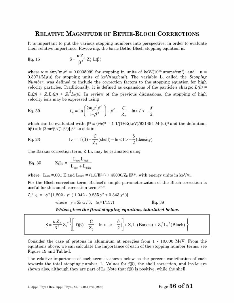
J. Appl. Phys / Rev. Appl. Phys., 85, 1249-1272 (1999) Page 36 of 51
RELATIVE MAGNITUDE OF BETHE-BLOCH CORRECTIONS It is important to put the various stopping numbers into perspective, in order to evaluate their relative importance. Reviewing, the basic Bethe-Bloch stopping equation is:
Eq. 15 SZ
Z L=κβ
β22 1
2 ( )
where κ ≡ 4πro2mec2 = 0.0005099 for stopping in units of keV/(1015 atoms/cm2), and κ = 0.3071/M2(u) for stopping units of keV/(mg/cm2). The variable L, called the Stopping Number, was defined to include the correction factors to the stopping equation for high velocity particles. Traditionally, it is defined as expansions of the particle’s charge: L(β) =
L0(β) + Z1L1(β) + Z12L2(β). In review of the previous discussions, the stopping of high
velocity ions may be expressed using
Eq. 39 2
ln1
2ln2
22
22
0δβ
ββ
−><−−−
−
= IZCcmL e
which can be evaluated with: β2 ≡ (v/c)2 = 1-1/[1+E(keV)/931494 M1(u)]2 and the definition: f(β) ≡ ln[2mc2β2/(1-β2)]-β2 to obtain:
Eq. 23 L0 = fCZ
shell I density( ) ( ) ln ( )βδ
− − < > −2 2
The Barkas correction term, Z1L1, may be estimated using
Eq. 35 Z1L1 = L L
L Llow high
low high+
where: Llow =.001 E and Lhigh = (1.5/E0.4) + 45000/Z2 E1.6 , with energy units in keV/u.
For the Bloch correction term, Bichsel’s simple parameterization of the Bloch correction is useful for this small correction term:27,84
Z12L2 = -y2 [1.202 - y2 ( 1.042 - 0.855 y2 + 0.343 y4 )]
where y ≡ Z1 α / β, (α=1/137) Eq. 38
Which gives the final stopping equation, tabulated below.
SZ
Z fCZ
I Z L Barkas Z L Bloch= − − < > −
+ +
κβ
βδ2
2 12
21 1 1
22
2
2( ) ln ( ) ( )
Consider the case of protons in aluminum at energies from 1 - 10,000 MeV. From the equations above, we can calculate the importance of each of the stopping number terms, see Figure 19 and Table-I.
The relative importance of each term is shown below as the percent contribution of each towards the total stopping number, L. Values for f(β), the shell correction, and ln<I> are shown also, although they are part of L0. Note that f(β) is positive, while the shell
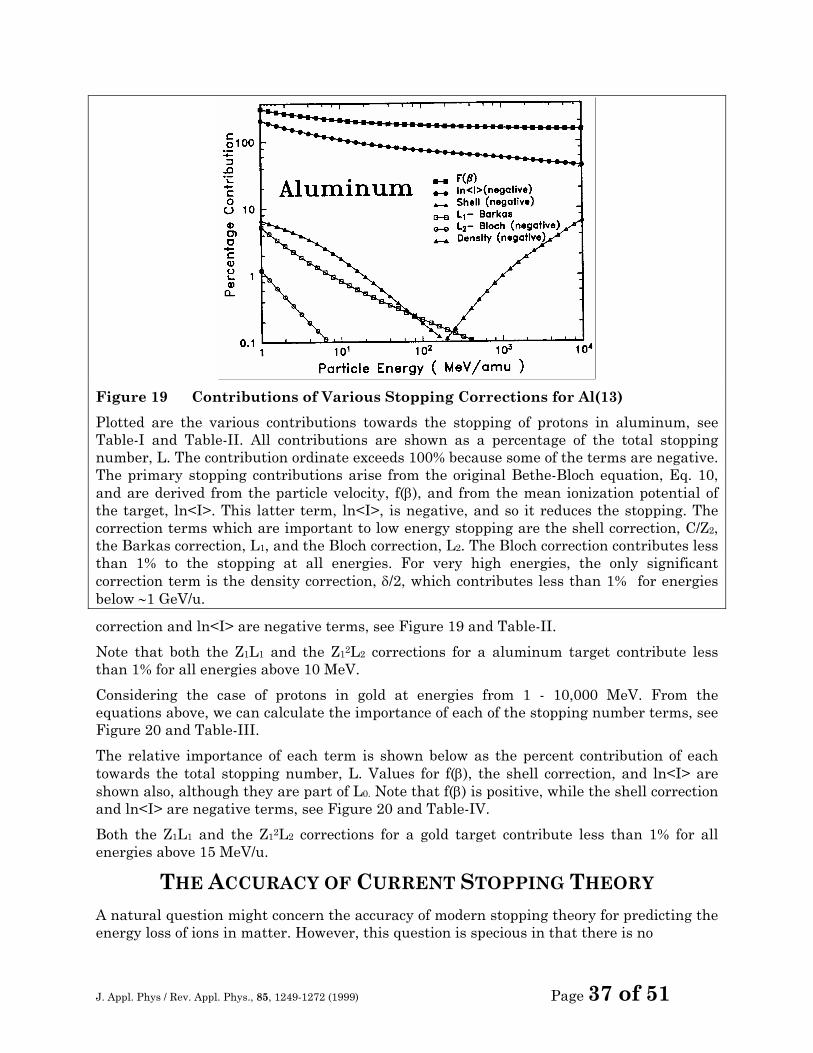
J. Appl. Phys / Rev. Appl. Phys., 85, 1249-1272 (1999) Page 37 of 51
Figure 19 Contributions of Various Stopping Corrections for Al(13)
Plotted are the various contributions towards the stopping of protons in aluminum, see Table-I and Table-II. All contributions are shown as a percentage of the total stopping number, L. The contribution ordinate exceeds 100% because some of the terms are negative. The primary stopping contributions arise from the original Bethe-Bloch equation, Eq. 10, and are derived from the particle velocity, f(β), and from the mean ionization potential of the target, ln<I>. This latter term, ln<I>, is negative, and so it reduces the stopping. The correction terms which are important to low energy stopping are the shell correction, C/Z2, the Barkas correction, L1, and the Bloch correction, L2. The Bloch correction contributes less than 1% to the stopping at all energies. For very high energies, the only significant correction term is the density correction, δ/2, which contributes less than 1% for energies below ∼1 GeV/u.
correction and ln<I> are negative terms, see Figure 19 and Table-II.
Note that both the Z1L1 and the Z12L2 corrections for a aluminum target contribute less than 1% for all energies above 10 MeV.
Considering the case of protons in gold at energies from 1 - 10,000 MeV. From the equations above, we can calculate the importance of each of the stopping number terms, see Figure 20 and Table-III.
The relative importance of each term is shown below as the percent contribution of each towards the total stopping number, L. Values for f(β), the shell correction, and ln<I> are shown also, although they are part of L0. Note that f(β) is positive, while the shell correction and ln<I> are negative terms, see Figure 20 and Table-IV.
Both the Z1L1 and the Z12L2 corrections for a gold target contribute less than 1% for all energies above 15 MeV/u.
THE ACCURACY OF CURRENT STOPPING THEORY A natural question might concern the accuracy of modern stopping theory for predicting the energy loss of ions in matter. However, this question is specious in that there is no
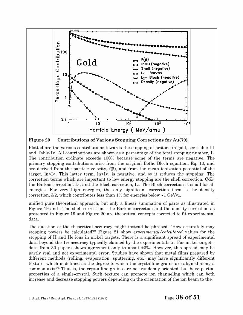
J. Appl. Phys / Rev. Appl. Phys., 85, 1249-1272 (1999) Page 38 of 51
Figure 20 Contributions of Various Stopping Corrections for Au(79)
Plotted are the various contributions towards the stopping of protons in gold, see Table-III and Table-IV. All contributions are shown as a percentage of the total stopping number, L. The contribution ordinate exceeds 100% because some of the terms are negative. The primary stopping contributions arise from the original Bethe-Bloch equation, Eq. 10, and are derived from the particle velocity, f(β), and from the mean ionization potential of the target, ln<I>. This latter term, ln<I>, is negative, and so it reduces the stopping. The correction terms which are important to low energy stopping are the shell correction, C/Z2, the Barkas correction, L1, and the Bloch correction, L2. The Bloch correction is small for all energies. For very high energies, the only significant correction term is the density correction, δ/2, which contributes less than 1% for energies below ∼1 GeV/u.
unified pure theoretical approach, but only a linear summation of parts as illustrated in Figure 19 and . The shell corrections, the Barkas correction and the density correction as presented in Figure 19 and Figure 20 are theoretical concepts corrected to fit experimental data.
The question of the theoretical accuracy might instead be phrased: "How accurately may stopping powers be calculated?" Figure 21 show experimental/calculated values for the stopping of H and He ions in nickel targets. There is a significant spread of experimental data beyond the 1% accuracy typically claimed by the experimentalists. For nickel targets, data from 30 papers shows agreement only to about ±3%. However, this spread may be partly real and not experimental error. Studies have shown that metal films prepared by different methods (rolling, evaporation, sputtering, etc.) may have significantly different texture, which is defined as the degree to which the crystalline grains are aligned along a common axis.85 That is, the crystalline grains are not randomly oriented, but have partial properties of a single-crystal. Such texture can promote ion channeling which can both increase and decrease stopping powers depending on the orientation of the ion beam to the
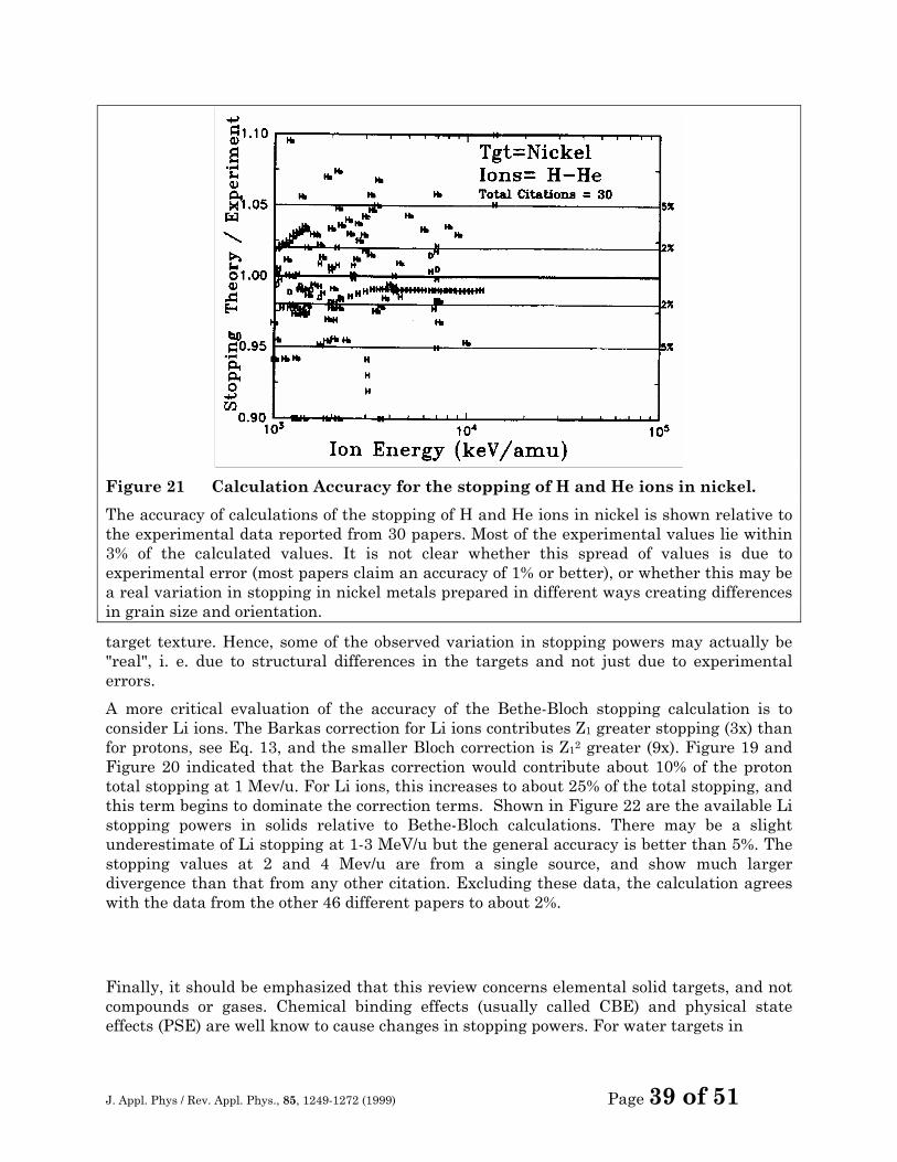
J. Appl. Phys / Rev. Appl. Phys., 85, 1249-1272 (1999) Page 39 of 51
Figure 21 Calculation Accuracy for the stopping of H and He ions in nickel.
The accuracy of calculations of the stopping of H and He ions in nickel is shown relative to the experimental data reported from 30 papers. Most of the experimental values lie within 3% of the calculated values. It is not clear whether this spread of values is due to experimental error (most papers claim an accuracy of 1% or better), or whether this may be a real variation in stopping in nickel metals prepared in different ways creating differences in grain size and orientation.
target texture. Hence, some of the observed variation in stopping powers may actually be "real", i. e. due to structural differences in the targets and not just due to experimental errors.
A more critical evaluation of the accuracy of the Bethe-Bloch stopping calculation is to consider Li ions. The Barkas correction for Li ions contributes Z1 greater stopping (3x) than for protons, see Eq. 13, and the smaller Bloch correction is Z12 greater (9x). Figure 19 and Figure 20 indicated that the Barkas correction would contribute about 10% of the proton total stopping at 1 Mev/u. For Li ions, this increases to about 25% of the total stopping, and this term begins to dominate the correction terms. Shown in Figure 22 are the available Li stopping powers in solids relative to Bethe-Bloch calculations. There may be a slight underestimate of Li stopping at 1-3 MeV/u but the general accuracy is better than 5%. The stopping values at 2 and 4 Mev/u are from a single source, and show much larger divergence than that from any other citation. Excluding these data, the calculation agrees with the data from the other 46 different papers to about 2%.
Finally, it should be emphasized that this review concerns elemental solid targets, and not compounds or gases. Chemical binding effects (usually called CBE) and physical state effects (PSE) are well know to cause changes in stopping powers. For water targets in
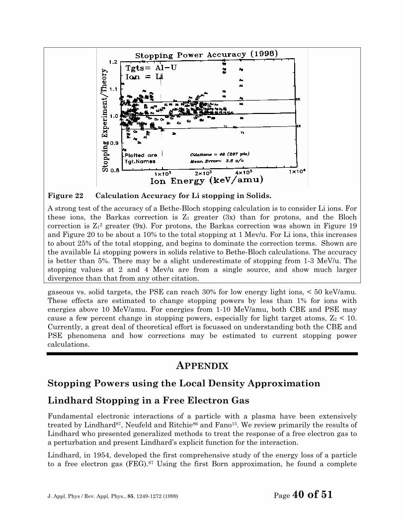
J. Appl. Phys / Rev. Appl. Phys., 85, 1249-1272 (1999) Page 40 of 51
Figure 22 Calculation Accuracy for Li stopping in Solids.
A strong test of the accuracy of a Bethe-Bloch stopping calculation is to consider Li ions. For these ions, the Barkas correction is Z1 greater (3x) than for protons, and the Bloch correction is Z12 greater (9x). For protons, the Barkas correction was shown in Figure 19 and Figure 20 to be about a 10% to the total stopping at 1 Mev/u. For Li ions, this increases to about 25% of the total stopping, and begins to dominate the correction terms. Shown are the available Li stopping powers in solids relative to Bethe-Bloch calculations. The accuracy is better than 5%. There may be a slight underestimate of stopping from 1-3 MeV/u. The stopping values at 2 and 4 Mev/u are from a single source, and show much larger divergence than that from any other citation.
gaseous vs. solid targets, the PSE can reach 30% for low energy light ions, < 50 keV/amu. These effects are estimated to change stopping powers by less than 1% for ions with energies above 10 MeV/amu. For energies from 1-10 MeV/amu, both CBE and PSE may cause a few percent change in stopping powers, especially for light target atoms, Z2 < 10. Currently, a great deal of theoretical effort is focussed on understanding both the CBE and PSE phenomena and how corrections may be estimated to current stopping power calculations.
APPENDIX
Stopping Powers using the Local Density Approximation
Lindhard Stopping in a Free Electron Gas
Fundamental electronic interactions of a particle with a plasma have been extensively treated by Lindhard87, Neufeld and Ritchie86 and Fano15. We review primarily the results of Lindhard who presented generalized methods to treat the response of a free electron gas to a perturbation and present Lindhard’s explicit function for the interaction.
Lindhard, in 1954, developed the first comprehensive study of the energy loss of a particle to a free electron gas (FEG).87 Using the first Born approximation, he found a complete
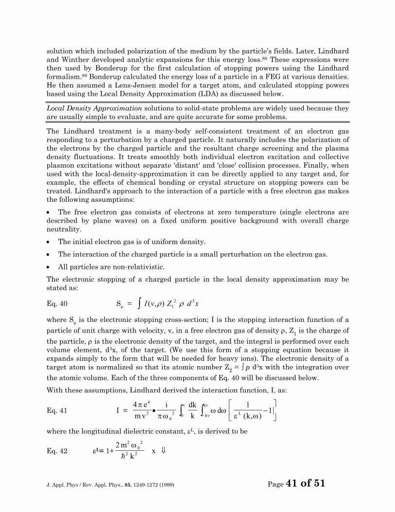
J. Appl. Phys / Rev. Appl. Phys., 85, 1249-1272 (1999) Page 41 of 51
solution which included polarization of the medium by the particle’s fields. Later, Lindhard and Winther developed analytic expansions for this energy loss.88 These expressions were then used by Bonderup for the first calculation of stopping powers using the Lindhard formalism.89 Bonderup calculated the energy loss of a particle in a FEG at various densities. He then assumed a Lens-Jensen model for a target atom, and calculated stopping powers based using the Local Density Approximation (LDA) as discussed below.
Local Density Approximation solutions to solid-state problems are widely used because they are usually simple to evaluate, and are quite accurate for some problems.
The Lindhard treatment is a many-body self-consistent treatment of an electron gas responding to a perturbation by a charged particle. It naturally includes the polarization of the electrons by the charged particle and the resultant charge screening and the plasma density fluctuations. It treats smoothly both individual electron excitation and collective plasmon excitations without separate 'distant' and 'close' collision processes. Finally, when used with the local-density-approximation it can be directly applied to any target and, for example, the effects of chemical bonding or crystal structure on stopping powers can be treated. Lindhard's approach to the interaction of a particle with a free electron gas makes the following assumptions:
• The free electron gas consists of electrons at zero temperature (single electrons are described by plane waves) on a fixed uniform positive background with overall charge neutrality.
• The initial electron gas is of uniform density.
• The interaction of the charged particle is a small perturbation on the electron gas.
• All particles are non-relativistic.
The electronic stopping of a charged particle in the local density approximation may be stated as:
Eq. 40 Se = I v Z d x( , )ρ ρ12 3∫
where Se is the electronic stopping cross-section; I is the stopping interaction function of a
particle of unit charge with velocity, v, in a free electron gas of density ρ, Z1 is the charge of
the particle, ρ is the electronic density of the target, and the integral is performed over each volume element, d3x, of the target. (We use this form of a stopping equation because it expands simply to the form that will be needed for heavy ions). The electronic density of a target atom is normalized so that its atomic number Z2 = ∫ p d3x with the integration over
the atomic volume. Each of the three components of Eq. 40 will be discussed below.
With these assumptions, Lindhard derived the interaction function, I, as:
Eq. 41 I = 4 1
14
20
2 0
ππω
ω ωε ω
em v
i dkk
dkLkv
kv• −
−
∞
∫∫ ( , )
where the longitudinal dielectric constant, εL, is derived to be
Eq. 42 εL= 1+2 2
02
2 2
mk
xω
h ⇓
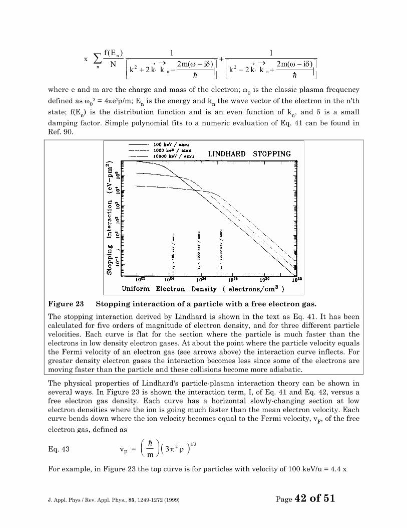
J. Appl. Phys / Rev. Appl. Phys., 85, 1249-1272 (1999) Page 42 of 51
x f E
Nk k k
m ik k k
m in
nn
n
( )( ) ( )
1
22
1
222 2+ ⋅
→−
−
+− ⋅
→+
−
→ →∑ ω δ ω δh h
where e and m are the charge and mass of the electron; ω0 is the classic plasma frequency
defined as ω02 = 4πe2ρ/m; En is the energy and kn the wave vector of the electron in the n'th
state; f(En) is the distribution function and is an even function of kn, and δ is a small
damping factor. Simple polynomial fits to a numeric evaluation of Eq. 41 can be found in Ref. 90.
Figure 23 Stopping interaction of a particle with a free electron gas.
The stopping interaction derived by Lindhard is shown in the text as Eq. 41. It has been calculated for five orders of magnitude of electron density, and for three different particle velocities. Each curve is flat for the section where the particle is much faster than the electrons in low density electron gases. At about the point where the particle velocity equals the Fermi velocity of an electron gas (see arrows above) the interaction curve inflects. For greater density electron gases the interaction becomes less since some of the electrons are moving faster than the particle and these collisions become more adiabatic.
The physical properties of Lindhard's particle-plasma interaction theory can be shown in several ways. In Figure 23 is shown the interaction term, I, of Eq. 41 and Eq. 42, versus a free electron gas density. Each curve has a horizontal slowly-changing section at low electron densities where the ion is going much faster than the mean electron velocity. Each curve bends down where the ion velocity becomes equal to the Fermi velocity, vF, of the free
electron gas, defined as
Eq. 43 vF = ( )h
m
3 2 1 3
π ρ/
For example, in Figure 23 the top curve is for particles with velocity of 100 keV/u = 4.4 x
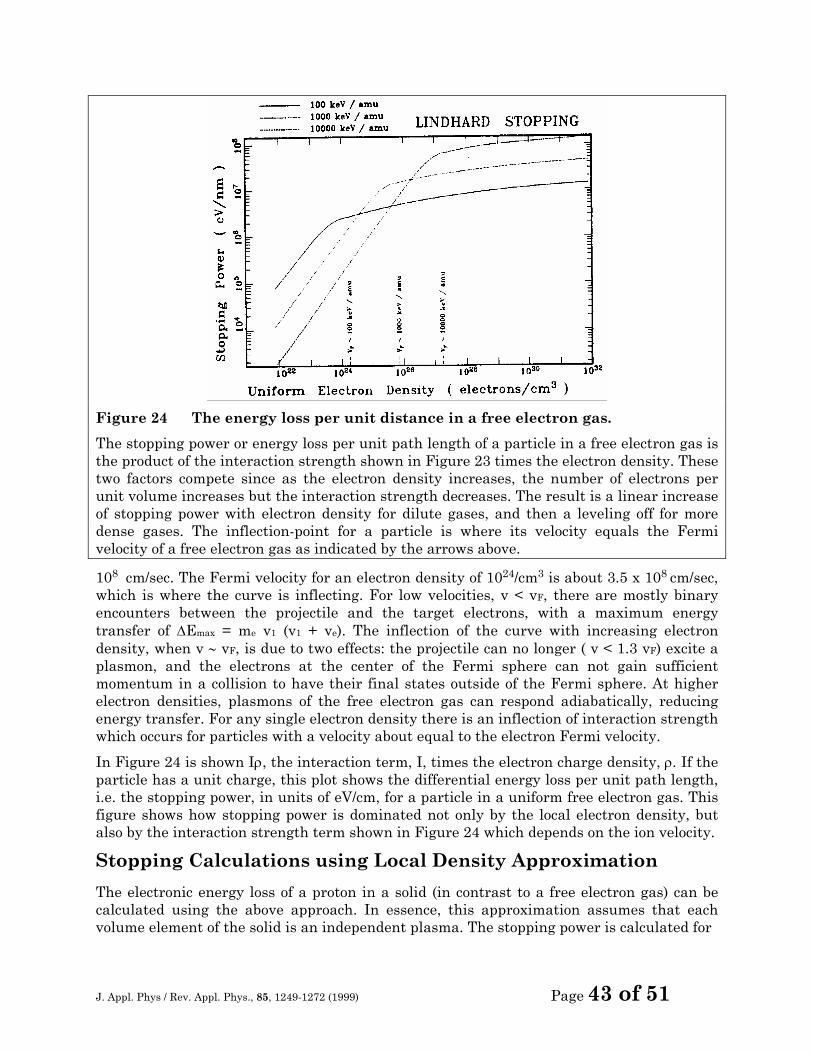
J. Appl. Phys / Rev. Appl. Phys., 85, 1249-1272 (1999) Page 43 of 51
Figure 24 The energy loss per unit distance in a free electron gas.
The stopping power or energy loss per unit path length of a particle in a free electron gas is the product of the interaction strength shown in Figure 23 times the electron density. These two factors compete since as the electron density increases, the number of electrons per unit volume increases but the interaction strength decreases. The result is a linear increase of stopping power with electron density for dilute gases, and then a leveling off for more dense gases. The inflection-point for a particle is where its velocity equals the Fermi velocity of a free electron gas as indicated by the arrows above.
108 cm/sec. The Fermi velocity for an electron density of 1024/cm3 is about 3.5 x 108 cm/sec, which is where the curve is inflecting. For low velocities, v < vF, there are mostly binary encounters between the projectile and the target electrons, with a maximum energy transfer of ∆Emax = me v1 (v1 + ve). The inflection of the curve with increasing electron density, when v ∼ vF, is due to two effects: the projectile can no longer ( v < 1.3 vF) excite a plasmon, and the electrons at the center of the Fermi sphere can not gain sufficient momentum in a collision to have their final states outside of the Fermi sphere. At higher electron densities, plasmons of the free electron gas can respond adiabatically, reducing energy transfer. For any single electron density there is an inflection of interaction strength which occurs for particles with a velocity about equal to the electron Fermi velocity.
In Figure 24 is shown Iρ, the interaction term, I, times the electron charge density, ρ. If the particle has a unit charge, this plot shows the differential energy loss per unit path length, i.e. the stopping power, in units of eV/cm, for a particle in a uniform free electron gas. This figure shows how stopping power is dominated not only by the local electron density, but also by the interaction strength term shown in Figure 24 which depends on the ion velocity.
Stopping Calculations using Local Density Approximation
The electronic energy loss of a proton in a solid (in contrast to a free electron gas) can be calculated using the above approach. In essence, this approximation assumes that each volume element of the solid is an independent plasma. The stopping power is calculated for
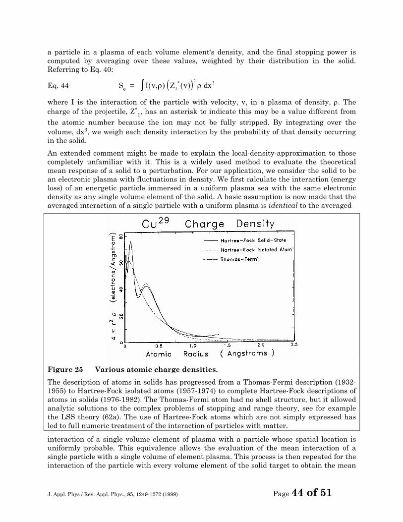
J. Appl. Phys / Rev. Appl. Phys., 85, 1249-1272 (1999) Page 44 of 51
a particle in a plasma of each volume element's density, and the final stopping power is computed by averaging over these values, weighted by their distribution in the solid. Referring to Eq. 40:
Eq. 44 Se = ( )I v Z v dx( , ) ( )*ρ ρ1
2 3∫
where I is the interaction of the particle with velocity, v, in a plasma of density, ρ. The charge of the projectile, Z*
1, has an asterisk to indicate this may be a value different from
the atomic number because the ion may not be fully stripped. By integrating over the volume, dx3, we weigh each density interaction by the probability of that density occurring in the solid.
An extended comment might be made to explain the local-density-approximation to those completely unfamiliar with it. This is a widely used method to evaluate the theoretical mean response of a solid to a perturbation. For our application, we consider the solid to be an electronic plasma with fluctuations in density. We first calculate the interaction (energy loss) of an energetic particle immersed in a uniform plasma sea with the same electronic density as any single volume element of the solid. A basic assumption is now made that the averaged interaction of a single particle with a uniform plasma is identical to the averaged
Figure 25 Various atomic charge densities.
The description of atoms in solids has progressed from a Thomas-Fermi description (1932-1955) to Hartree-Fock isolated atoms (1957-1974) to complete Hartree-Fock descriptions of atoms in solids (1976-1982). The Thomas-Fermi atom had no shell structure, but it allowed analytic solutions to the complex problems of stopping and range theory, see for example the LSS theory (62a). The use of Hartree-Fock atoms which are not simply expressed has led to full numeric treatment of the interaction of particles with matter.
interaction of a single volume element of plasma with a particle whose spatial location is uniformly probable. This equivalence allows the evaluation of the mean interaction of a single particle with a single volume of element plasma. This process is then repeated for the interaction of the particle with every volume element of the solid target to obtain the mean
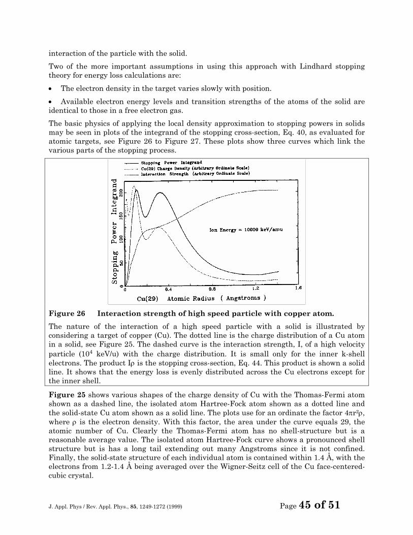
J. Appl. Phys / Rev. Appl. Phys., 85, 1249-1272 (1999) Page 45 of 51
interaction of the particle with the solid.
Two of the more important assumptions in using this approach with Lindhard stopping theory for energy loss calculations are:
• The electron density in the target varies slowly with position.
• Available electron energy levels and transition strengths of the atoms of the solid are identical to those in a free electron gas.
The basic physics of applying the local density approximation to stopping powers in solids may be seen in plots of the integrand of the stopping cross-section, Eq. 40, as evaluated for atomic targets, see Figure 26 to Figure 27. These plots show three curves which link the various parts of the stopping process.
Figure 26 Interaction strength of high speed particle with copper atom.
The nature of the interaction of a high speed particle with a solid is illustrated by considering a target of copper (Cu). The dotted line is the charge distribution of a Cu atom in a solid, see Figure 25. The dashed curve is the interaction strength, I, of a high velocity particle (104 keV/u) with the charge distribution. It is small only for the inner k-shell electrons. The product Iρ is the stopping cross-section, Eq. 44. This product is shown a solid line. It shows that the energy loss is evenly distributed across the Cu electrons except for the inner shell.
Figure 25 shows various shapes of the charge density of Cu with the Thomas-Fermi atom shown as a dashed line, the isolated atom Hartree-Fock atom shown as a dotted line and the solid-state Cu atom shown as a solid line. The plots use for an ordinate the factor 4πr2ρ, where ρ is the electron density. With this factor, the area under the curve equals 29, the atomic number of Cu. Clearly the Thomas-Fermi atom has no shell-structure but is a reasonable average value. The isolated atom Hartree-Fock curve shows a pronounced shell structure but is has a long tail extending out many Angstroms since it is not confined. Finally, the solid-state structure of each individual atom is contained within 1.4 Å, with the electrons from 1.2-1.4 Å being averaged over the Wigner-Seitz cell of the Cu face-centered-cubic crystal.
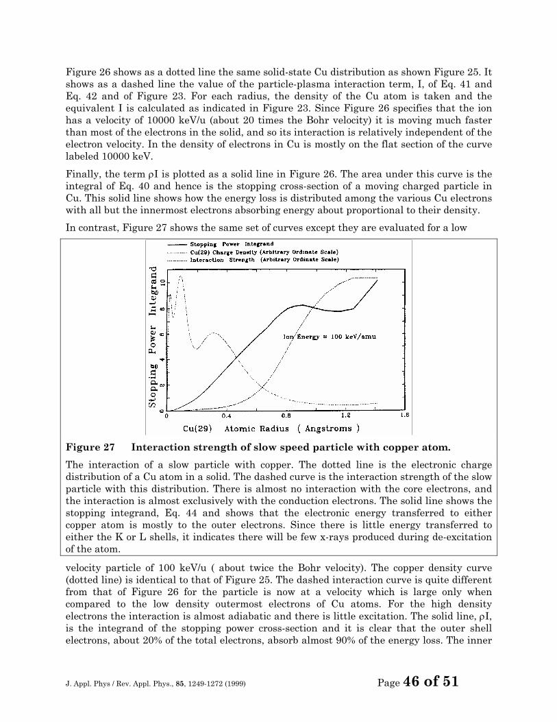
J. Appl. Phys / Rev. Appl. Phys., 85, 1249-1272 (1999) Page 46 of 51
Figure 26 shows as a dotted line the same solid-state Cu distribution as shown Figure 25. It shows as a dashed line the value of the particle-plasma interaction term, I, of Eq. 41 and Eq. 42 and of Figure 23. For each radius, the density of the Cu atom is taken and the equivalent I is calculated as indicated in Figure 23. Since Figure 26 specifies that the ion has a velocity of 10000 keV/u (about 20 times the Bohr velocity) it is moving much faster than most of the electrons in the solid, and so its interaction is relatively independent of the electron velocity. In the density of electrons in Cu is mostly on the flat section of the curve labeled 10000 keV.
Finally, the term ρI is plotted as a solid line in Figure 26. The area under this curve is the integral of Eq. 40 and hence is the stopping cross-section of a moving charged particle in Cu. This solid line shows how the energy loss is distributed among the various Cu electrons with all but the innermost electrons absorbing energy about proportional to their density.
In contrast, Figure 27 shows the same set of curves except they are evaluated for a low
Figure 27 Interaction strength of slow speed particle with copper atom.
The interaction of a slow particle with copper. The dotted line is the electronic charge distribution of a Cu atom in a solid. The dashed curve is the interaction strength of the slow particle with this distribution. There is almost no interaction with the core electrons, and the interaction is almost exclusively with the conduction electrons. The solid line shows the stopping integrand, Eq. 44 and shows that the electronic energy transferred to either copper atom is mostly to the outer electrons. Since there is little energy transferred to either the K or L shells, it indicates there will be few x-rays produced during de-excitation of the atom.
velocity particle of 100 keV/u ( about twice the Bohr velocity). The copper density curve (dotted line) is identical to that of Figure 25. The dashed interaction curve is quite different from that of Figure 26 for the particle is now at a velocity which is large only when compared to the low density outermost electrons of Cu atoms. For the high density electrons the interaction is almost adiabatic and there is little excitation. The solid line, ρI, is the integrand of the stopping power cross-section and it is clear that the outer shell electrons, about 20% of the total electrons, absorb almost 90% of the energy loss. The inner
J. Appl. Phys / Rev. Appl. Phys., 85, 1249-1272 (1999) Page 47 of 51
k-shell electrons absorb almost no energy and one would anticipate that there would be almost no k-shell x-rays emitted from the Cu target.
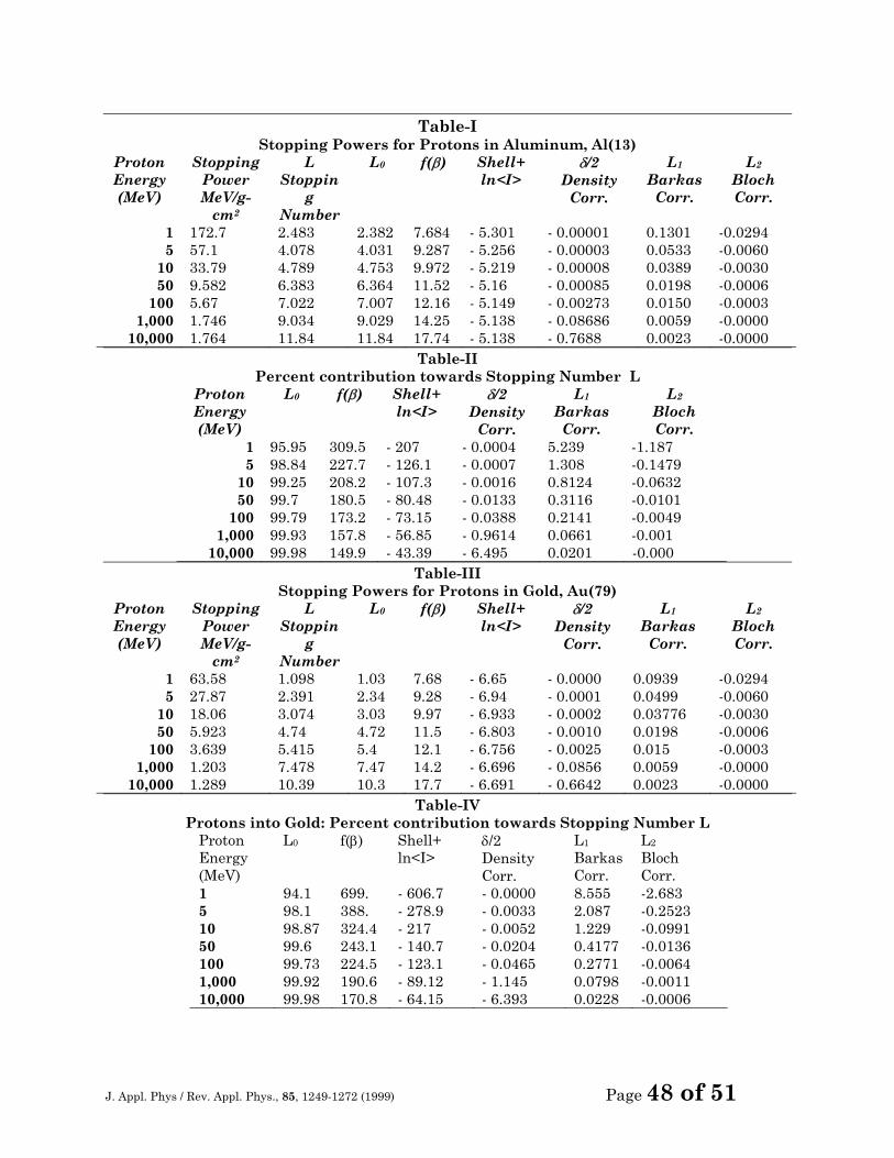
J. Appl. Phys / Rev. Appl. Phys., 85, 1249-1272 (1999) Page 48 of 51
Table-I Stopping Powers for Protons in Aluminum, Al(13)
Proton Energy (MeV)
Stopping Power MeV/g-
cm2
L Stoppin
g Number
L0 f(β) Shell+ ln<I>
δ/2 Density
Corr.
L1 Barkas Corr.
L2 Bloch Corr.
1 172.7 2.483 2.382 7.684 - 5.301 - 0.00001 0.1301 -0.0294 5 57.1 4.078 4.031 9.287 - 5.256 - 0.00003 0.0533 -0.0060
10 33.79 4.789 4.753 9.972 - 5.219 - 0.00008 0.0389 -0.0030 50 9.582 6.383 6.364 11.52 - 5.16 - 0.00085 0.0198 -0.0006
100 5.67 7.022 7.007 12.16 - 5.149 - 0.00273 0.0150 -0.0003 1,000 1.746 9.034 9.029 14.25 - 5.138 - 0.08686 0.0059 -0.0000
10,000 1.764 11.84 11.84 17.74 - 5.138 - 0.7688 0.0023 -0.0000 Table-II
Percent contribution towards Stopping Number L Proton Energy (MeV)
L0 f(β) Shell+ ln<I>
δ/2 Density
Corr.
L1 Barkas Corr.
L2 Bloch Corr.
1 95.95 309.5 - 207 - 0.0004 5.239 -1.187 5 98.84 227.7 - 126.1 - 0.0007 1.308 -0.1479
10 99.25 208.2 - 107.3 - 0.0016 0.8124 -0.0632 50 99.7 180.5 - 80.48 - 0.0133 0.3116 -0.0101
100 99.79 173.2 - 73.15 - 0.0388 0.2141 -0.0049 1,000 99.93 157.8 - 56.85 - 0.9614 0.0661 -0.001
10,000 99.98 149.9 - 43.39 - 6.495 0.0201 -0.000 Table-III
Stopping Powers for Protons in Gold, Au(79) Proton Energy (MeV)
Stopping Power MeV/g-
cm2
L Stoppin
g Number
L0 f(β) Shell+ ln<I>
δ/2 Density
Corr.
L1 Barkas Corr.
L2 Bloch Corr.
1 63.58 1.098 1.03 7.68 - 6.65 - 0.0000 0.0939 -0.0294 5 27.87 2.391 2.34 9.28 - 6.94 - 0.0001 0.0499 -0.0060
10 18.06 3.074 3.03 9.97 - 6.933 - 0.0002 0.03776 -0.0030 50 5.923 4.74 4.72 11.5 - 6.803 - 0.0010 0.0198 -0.0006
100 3.639 5.415 5.4 12.1 - 6.756 - 0.0025 0.015 -0.0003 1,000 1.203 7.478 7.47 14.2 - 6.696 - 0.0856 0.0059 -0.0000
10,000 1.289 10.39 10.3 17.7 - 6.691 - 0.6642 0.0023 -0.0000 Table-IV
Protons into Gold: Percent contribution towards Stopping Number L Proton Energy (MeV)
L0 f(β) Shell+ ln<I>
δ/2 Density Corr.
L1 Barkas Corr.
L2 Bloch Corr.
1 94.1 699. - 606.7 - 0.0000 8.555 -2.683 5 98.1 388. - 278.9 - 0.0033 2.087 -0.2523 10 98.87 324.4 - 217 - 0.0052 1.229 -0.0991 50 99.6 243.1 - 140.7 - 0.0204 0.4177 -0.0136 100 99.73 224.5 - 123.1 - 0.0465 0.2771 -0.0064 1,000 99.92 190.6 - 89.12 - 1.145 0.0798 -0.0011 10,000 99.98 170.8 - 64.15 - 6.393 0.0228 -0.0006
J. Appl. Phys / Rev. Appl. Phys., 85, 1249-1272 (1999) Page 49 of 51
References
1 Mme. Pierre Curie, Comptes Rendus, 130, 76 (1900). 2 J. J. Thomson, "Conduction of Electricity through Gases", Cambridge University
Press (1903). 3 H. Gieger and E. Marsden, Proc. Roy. Soc., 82, 495 (1909). 4 E. Rutherford, Phil. Mag., 21, 212 (1911); ibid. 21, 699 (1911). 5 J. J. Thomson, Phil. Mag., 6-23, 449 (1912). 6 N. Bohr, Phil. Mag., 25, 10 (1913). 7 N. Bohr, Phil. Mag., 30, 581 (1915). 8 H. Bethe, Ann. Physik, 5, 325 (1930). 9 H. Bethe, Z. Phys., 76, 293 (1932). 10 F. Bloch, Ann. Phys., 16, 285 (1933). 11 F. Bloch, Z. Phys., 81, 363 (1933). 12 U. Fano, Ann. Rev. Nucl. Sci., 13, 1 (1963). This extended work is based on earlier
papers:); U. Fano, Phys. Rev. 13 U. Fano, Phys. Rev., 72, 26 (1947). 14 U. Fano, Phys. Rev., 102, 385 (1956). 15 U. Fano, Phys. Rev., 103, 1202 (1956). 16 U. Fano, Ann. Rev. Nucl. Sci., 13, 67 (1963). This paper can also be found in
reference 22, included as Appendix A. 17 M. Inokuti, Rev. Mod. Phys., 43, 297 (1971) 18 H. Bichsel, Amer. Inst. of Physics Handbook, McGraw-Hill, New York, 8-142 (1972). 19 P. Sigmund, Radiation Damage Processes in Materials, C. duPuy, ed., Noordhoff,
Leiden, 3 (1975). 20 J. D. Jackson, Classical Electrodynamics, 2nd Ed., Wiley, New York, Chap. 13, 15
(1975). 21 S. P. Ahlen, Rev. Mod. Phys., vol. 52, 121 (1980). 22 U. Fano, Chr., Studies in Penetration of Charged Particles in Matter, Nucl. Sci. Rpt..
39, U. S. National Academy of Sciences, Washington, 1-338 (1964). 23 L. C. Northcliffe and R. F. Schilling, Nucl. Data Tables, 7, 233-463 (1970). 24 J. F. Janni, Atom. Data and Nucl. Data Tables, vol. 27, (1982). Two volumes. 25 H. H. Andersen and J. F. Ziegler, Hydrogen Stopping Powers and Ranges in All
Elements, Pergamon, New York (1977). 26 J. F. Ziegler, Helium Stopping Powers and Ranges in All Elemental Matter,
Pergamon, New York (1977). 27 ICRU-49, H. O. Wyckoff (ICRU Scientific Counsellor), “Stopping Powers and Ranges
for Protons and Alpha Particles”, Intl. Comm. on Rad. Units, Bethseda, MD (1993). 28 G. H. Henderson, Phil. Mag., vol. 44, 680 (1922). 29 I. A. Gaunt, Proc. Camb. Phil. Soc., vol. 23, 732 (1927). 30 N. F. Mott, Proc. Camb. Phil. Soc., vol. 27, 553 (1931). 31 C. Moller, Ann. Physik, vol. 14, 531 (1932). 32 J. J. Thomson, “Conduction of Electricity Through Gases”, Cambridge University
Press, (1903). J. J. Thomson, Phil. Mag., 6-23, 449 (1912). 33 E. Rutherford, Phil. Mag., 21, 212 (1911); ibid 21, 699 (1911). 34 N. Bohr, Phil. Mag., 25, 10 (1913).
J. Appl. Phys / Rev. Appl. Phys., 85, 1249-1272 (1999) Page 50 of 51
35 W. E. Lamb, Phys. Rev., 58, 696 (1940). 36 N. Bohr, Phys. Rev., 58, 654 (1940). 37 N. Bohr, Phys. Rev., 59, 279 (1941). 38 L. C. Northcliffe, Phys. Rev., 120, 1744 (1960). 39 N. Bohr, Kgl. Dansk. Vid. Sel., Mat.-Fys. Medd., 18, 1 (1948). 40 M. C. Walske, Phys. Rev., 88, 1283 (1952), and Phys. Rev., 101, 940 (1956). 41 M. C. Walske, Phys. Rev., 101, 940 (1956). 42 G. S. Khandelwal, Nucl. Phys., A116, 97 (1968). 43 H. Bichsel, Univ. of Calif. Rpt. USC-136-120. 44 G. S. Khandelwal and E. Merzbacher, Phys. Rev., 144, 349 (1966). 45 H. Bichsel, Studies in Penetration of Charged Particles in Matter, U. S. Natl. Acad.
Sci., Pub. 1133, 17-38 (1964). 46 H. Bichsel, Amer. Inst. Phys. Handbook, McGraw Hill, New York, 8-142 (1972). 47 H. Bichsel, Phys. Rev. A, 28, 1147 (1983). 48 H. Bichsel, Phys. Rev. A, 46, 5761 (1992). Includes citations to numerous prior
calculations. 49 C. C. Rousseau, W. K. Chu and D. Powers, Phys. Rev., A4, 1066 (1970). 50 J. F. Ziegler, “Handbook of Stopping Cross-Sections for Energetic Ions in All
Elements”, Pergamon Press (1980). 51 J. Lindhard and M. Scharff, Mat. Fys. Medd. Dan. Vid. Selsk., 27, No. 15 (1952). 52 W. K. Chu and D. Powers, Phys. Lett., 40A, 23 (1972). 53 W. F. G. Swann, J. Franklin Inst., 226, 598 (1938). 54 E. Fermi, Phys. Rev., 57, 485 (1940), 55 R. M. Sternheimer, Phys. Rev., 117, 485 (1960). 56 R. M. Sternheimer, Phys. Rev., 145, 247 (1966). 57 R. M. Sternheimer, S. M. Seltzer and M. J. Berger, Phys. Rev., B26, 6067 (1982). 58 A. Crispin and G. N. Fowler, Rev. Mod. Phys., 42, 290 (1970). 59 M. Inokuti and D. Y. Smith, Phys. Rev., B25, 61 (1982). 60 J. C. Ashley, Radiat. Res., 89, 32 (1982). 61 H. Bichsel, Rev. Mod. Phys., 60, 663 (1988). 62 ICRU Report #37, H. O. Wyckoff (ICRU Scientific Counsellor), “Stopping Powers for
Electrons and Positrons”, Intl. Comm. on Rad. Units, Bethseda, MD (1984). 63 W. H. Barkas, W. Birnbaum and F. M. Smith, Phys. Rev., 101, 778 (1956). 64 W. H. Barkas, N. J. Dyer and H. H. Heckmann, Phys. Rev. Lett., 11, 26 (1963). 65 H. H. Heckman, “Penetration of Charged Particles in Matter”, U.S. National
Academy of Science Report # 1133, Washington, D.C., 41 (1970). 66 J. C. Ashley, R. H. Ritchie and W. Brandt, Phys. Rev., B5, 2393 (1972). 67 J. C. Ashley, R. H. Ritchie and W. Brandt, Phys. Rev., A8, 2404 (1973) 68 J. C. Ashley, V. E. Anderson, R. H. Ritchie and W. Brandt, National Auxiliary
Publication Service, New York. 69 J. D. Jackson and R. L. McCarthy, Phys. Rev., B6, 4131 (1972). 70 K. W. Hill and E. Merzbacher, Phys. Rev., A9, 156 (1974). 71 J. Lindhard, Nucl. Inst. Methods, 132,1 (1976). 72 R. Medenwaldt, S. P. Moller, E. Uggerhoj, T. Worm, P. Hvelplund, H. Knudsen and
K. Eksener, Nucl. Inst. Methods, B58, 1 (1991), and Phys. Rev. Lett., A155, 155 (1991)..
73 H. H. Andersen, J. F. Bak, H. Knudsen, P. Moller-Petersen and B. R. Nielsen,
J. Appl. Phys / Rev. Appl. Phys., 85, 1249-1272 (1999) Page 51 of 51
“Physics of Ionized Gases”, Navinsek (ed.), J. Stefan Institute, Ljubljana, 221 (1976). H. H. Andersen, J. F. Bak, H. Knudsen, and B. R. Nielsen, Phys. Rev., A16, 1929 (1977). H. H. Andersen, Physica Scripta, 28, 268 (1983).
74 H. H. Mikkelsen and P. Sigmund, Phys. Rev., A40, 101 (1989). 75 H. H. Mikkelsen and E. H. Mortensen, Nucl. Inst. Methods, B48, 39 (1990). 76 H. Esbensen and P. Sigmund, Ann. Physics, 201, 152 (1990). See also: H. Esbensen,
Ph. D. Thesis, Odense University, Denmark (1991). 77 H. H. Mikkelsen, H. Exbensen and P. Sigmund, Nucl. Inst. Methods, B48, 8 (1990). 78 H. H. Mikkelsen and H. Flyvbjerg, Phys. Rev., A45, 3025 (1992). 79 P. Sigmund, Nucl. Inst. Methods, B85, 541 (1994). 80 L. H. Andersen, P. Hvelplund, H.. Knudsen, S. P. Moller, J. O. P. Pedersen, E.
Uggerhoj, K. Elsener and E. Morenzoni, Phys. Rev. Lett., 62, 1731 (1989). 81 H. Bichsel and L. E. Porter, Phys. Rev., A25, 2499 (1982). 82 H. H. Andersen, J. F. Bak, H. Knudsen and B. R. Nielsen, Phys. Rev., A16, 1929
(1977). 83 H. Bichsel, Phys. Rev., A41, 3642 (1990). 84 H. Bichsel, Phys. Rev., A41, 3642 (1990). 85 H. H. Andersen, K. N. Tu and J. F. Ziegler, Nucl. Inst. Methods, 149, 247-251 (1978). 86 J. Neufeld and R. H. Ritchie, Phys. Rev., 98, 1632 (1955). 87 J. Lindhard, Mat. Fys. Medd. Dan. Vid. Selsk., 28, No. 8 (1954). 88 J. Lindhard and A. Winther, Mat. Fys. Medd. Dan. Vid. Selsk., 34, No. 4 (1964). 89 E. Bonderup, Mat. Fys. Medd. Dan. Vid. Selsk., 35, No. 17 (1967). 90 G. J. Iafrate and J. F. Ziegler, J. Appl. Phys., 50, 5579 (1979) plus errata available
from the authors.