The Stochastic Human Exposure and Dose Si

for Multimedia, Multipathway Chemicals (SHEDS-Multimedia):Dietary Module

mulation Model

SHEDS-Dietary version 1

User Guide

June 4, 2012

Prepared by: Kristin Isaacs1, Jianping Xue1, Casson Stallings2, and Valerie Zartarian1 1 US Environmental Protection Agency, Office of Research and Development, National Exposure Research Laboratory 2Alion Science and Technology

i

TABLE OF CONTENTS LIST OF FIGURES ................................................................................................................... iii LIST OF TABLES ...................................................................................................................... v Acknowledgments ...................................................................................................................... vi Computing Issues, Disclaimer, and Support ............................................................................... vii ACRONYMS AND ABBREVIATIONS .................................................................................. viii 1 Overview of SHEDS-Dietary .................................................................................................1 2 Version History .....................................................................................................................1 3 Installation .............................................................................................................................2

3.1 Requirements .......................................................................................................2 3.2 Installation under MS Windows ............................................................................3

3.2.1 Starting with a CD...................................................................................3 3.2.2 Starting with a Downloaded File ..............................................................3 3.2.3 The Standard Installation Process ............................................................3 3.2.4 Starting the Model Interface ....................................................................6 3.2.5 Removing SHEDS-Dietary ......................................................................7

4 The SAS User Interface .........................................................................................................8 4.1 The SAS Screen ...................................................................................................8

5 General Interface Hints ........................................................................................................ 11 5.1 Display Issues ..................................................................................................... 11 5.2 Grayed Out Buttons or Widgets ......................................................................... 11

6 SHEDS-Dietary: The Graphical User Interface .................................................................... 12 6.1 Overview of the SHEDS-Dietary Interface ......................................................... 12 6.2 SHEDS-Dietary Main Interface Screen ............................................................... 13 6.3 Specify Run File ................................................................................................. 14 6.4 Main Simulation Settings .................................................................................... 15 6.5 Import and Enter Residue File ............................................................................ 22

6.5.1 The Residue File Editor and Residue File Format ................................... 22 6.5.2 Importing and Editing a Residue File ..................................................... 24 6.5.3 Creating a New Residue File .................................................................. 25 6.5.4 Validating a Residue File ....................................................................... 25

6.6 Assign Residues to Commodities ........................................................................ 26 6.6.1 Overview of the Assign Residues to Commodity Screen Options ........... 26 6.6.2 Assigning Residues to Commodities ...................................................... 28 6.6.3 Validating the Residue Data .................................................................. 29

6.7 Set Up and Run SHEDS-Dietary Module ........................................................... 32 6.7.1 Other Options........................................................................................ 33 6.7.2 Risk (Toxicological) Parameters ............................................................ 33

6.8 Pre-Process Output Data .................................................................................... 35 6.9 View Results ...................................................................................................... 38

6.9.1 The View Cross-Sectional Results Window ........................................... 38 6.9.2 CDFs..................................................................................................... 40

ii

6.9.3 Exposure: Percentile Table .................................................................... 41 6.9.4 Exposure and aPAD: Summary Table .................................................... 43 6.9.5 Contribution by Commodity: Bar Chart or Pie Chart.............................. 44 6.9.6 Contribution by Commodity: Summary Table ........................................ 46 6.9.7 View Longitudinal Results ..................................................................... 48

7 PDP Generator .................................................................................................................... 51 8 Example Case Studies .......................................................................................................... 53

8.1 Case Study 2: Cis-Permethrin, Cross-Sectional Run ............................................ 53 8.2 Case Study 3: Cis-Permethrin, Longitudinal Run ................................................ 65 8.3 Case Study 4: Pyrethroids, Cross-Sectional Run ................................................. 73

9 References ........................................................................................................................... 86 Appendix A. Directories, Libraries, and Files ............................................................................. 87

A.1 Directories/Libraries ........................................................................................... 87 A.2 Input Files .......................................................................................................... 88

A.2.1 The Run Information File ...................................................................... 88 A.2.2 Final (Processed) Residue Files for Single Chemicals ............................. 90 A.2.3 Final (Processed) Residue Files for Multiple Chemicals .......................... 91 A.2.4 Bridge Files for Multiple Chemicals ....................................................... 93 A.2.5 Processing Factor Files (Multiple Chemicals) ......................................... 95 A.2.6 Chemical Code Files (Multiple Chemicals) ............................................. 96

A.3 Output Files ....................................................................................................... 97 A.3.1 Cross-Sectional Output Datasets ........................................................... 98 A.3.2 Longitudinal Output Datasets ................................................................ 99 A.3.3 Summary Output Datasets ..................................................................... 99

iii

LIST OF FIGURES Figure 3-1. Setup Screens: Initial Screen. .....................................................................................4Figure 3-2. Setup Screens: Welcome and Information Screen. .....................................................4Figure 3-3. Setup Screens: Installation Directory Screen. .............................................................5Figure 3-4. Setup Screens: Shortcut Folder Name. .......................................................................5Figure 3-5. Setup Screens: Confirmation Screen. .........................................................................6Figure 3-6. Setup Screens: Completion Confirmation. ..................................................................6Figure 3-7. SHEDS Dietary Desktop Icon. ..................................................................................6Figure 4-1. The Main SHEDS-Dietary Interface Screen in the SAS Window on Startup. .............9Figure 4-2. The SAS Menu Bar and the View Menu. ...................................................................9Figure 4-3. The SAS Explorer Window. .................................................................................... 10Figure 5-1. Sample of Two Buttons, One Normal and One Grayed Out (Bottom). ..................... 11Figure 6-1. Overview of the SHEDS-Dietary Interface. ............................................................. 12Figure 6-2. SHEDS-Dietary Main Screen. ................................................................................. 13Figure 6-3. The Specify Run Screen. .......................................................................................... 14Figure 6-4. Selecting a Run File. ................................................................................................ 14Figure 6-5. The Main Simulation Settings Screen. ...................................................................... 16Figure 6-6. The Study Design Options for a Longitudinal Run. .................................................. 16Figure 6-7. The Chemical Information Section of the Main Simulation Settings Screen for a

Cumulative Simulation. ...................................................................................................... 17Figure 6-8. The Second Main Settings Screen for Single-Chemical Runs. .................................. 18Figure 6-9. The Second Main Settings Screen for Multi-Chemical (Cumulative) Runs. ............... 20Figure 6-10. Longitudinal Settings Screen. ................................................................................ 21Figure 6-11. The Residue File Editor Screen. ............................................................................. 23Figure 6-12. Assign Residues to Food Commodities Screen. ...................................................... 27Figure 6-13. The Select One or More Commodities Widget when Food Form Variables (Cooking

Method, Cooking Status, and Food Form) are Selected. .................................................... 28Figure 6-14. Residue File Selection Box .................................................................................... 29Figure 6-15. The SHEDS Error Screen. ..................................................................................... 31Figure 6-16. The Run SHEDS-Dietary Screen for Single and Multichemical Cross-Sectional Runs

.......................................................................................................................................... 32Figure 6-17. Run Screen Error Field .......................................................................................... 34Figure 6-18. Check Run Variables ............................................................................................. 35Figure 6-19. The Preprocess Output Data Screen. ..................................................................... 36Figure 6-20. The View Results Screen. ...................................................................................... 38Figure 6-21. The View Cross-Sectional Results Control Section ................................................ 39Figure 6-22. Example of a CDF Plot Created with View Results ................................................ 41Figure 6-23. Example of an Exposure Percentile Table .............................................................. 42Figure 6-24. Example of an Exposure and %APAD Summary Table .......................................... 43Figure 6-25. Example of a Contribution by Commodity Bar Chart ............................................. 45Figure 6-26. Example of a Contribution by Commodity Pie Chart .............................................. 46Figure 6-27. Example of a Contribution by Commodity Summary Table .................................... 47Figure 6-28. The Control Section of the View Longitudinal Results Window ............................. 48Figure 6-29. A Daily Exposure Time-Series for a Longitudinal Run. .......................................... 49

iv

Figure 6-30. A Persistent Exposure Time Series Added to a Longitudinal Plot. .......................... 50Figure 7-1. The PDP Generator Screen. ..................................................................................... 51 Figure A-1. An Example Single-Chemical Residue File. ............................................................ 91 Figure A-2. A Final Residue File for Multiple Chemicals (Pyrethroids). ..................................... 92 Figure A-3. A Pesticide Code File for Pyrethroids ..................................................................... 93 Figure A-4. Example Bridge File for Multiple Chemicals........................................................... 94 Figure A-5. Example Processing Factor File ............................................................................. 96 Figure A-6. Example Chemical Code File ................................................................................. 97

v

LIST OF TABLES Table 6-1. Risk (Toxicological) Parameters in the Run Information File ..................................... 34 Table A-1. SHEDS-Dietary Directories and Libraries ............................................................... 87 Table A-2. Variables in the Run Information File ..................................................................... 88 Table A-3. Variables in the Final Residue File for Single Chemicals .......................................... 90 Table A-4. Variables in the Final Residue File for Multiple Chemicals ....................................... 92 Table A-5. Variables in the Final Residue File for Multiple Chemicals (Pyrethroids) ................. 93 Table A-6. Variables in the Bridge File for Multiple Chemicals ................................................. 94 Table A-7. Variables in the Processing Factor File for Multiple Chemicals ................................ 95 Table A-8. Variables in the Chemical Code File for Multiple Chemicals .................................... 96 Table A-9. Variables in the Cross-Sectional Output Datasets .................................................... 98 Table A-10. Variables in the Longitudinal Output Datasets ....................................................... 99

vi

Acknowledgments We would like to thank our colleagues in EPA’s Office of Pesticide Programs, and Dr. Andrew Geller in EPA's Office of Research and Development, for their input into the SHEDS-Dietary Graphical User Interface design and their review of this User Guide.

vii

Computing Issues, Disclaimer, and Support Computing Issues It is strongly advised that the SHEDS user maximize windows so that as much as possible of the full dialog is displayed. You may still need to scroll down to see all of some dialogs. Refer to the images in this User Guide to ensure that all components of a dialog are displayed. It is recommended that the user’s display have a resolution of at least It is highly recommended that the user pause or disable any automated anti-virus or back-up programs that access the SHEDS installation or data output directories, or place these directories in locations that are not virus-checked or backed up. Such programs may access SHEDS data files and interfere with model performance, causing unpredictable results. Disclaimer EPA's SHEDS-Dietary model is a probabilistic, population-based dietary exposure assessment model that simulates individual exposures to chemicals in food and drinking water over different time periods (e.g., daily, yearly). SHEDS-Dietary is one module (along with the separate SHEDS-Residential module) of EPA’s more comprehensive human exposure model, the Stochastic Human Exposure and Dose Simulation model for multimedia, multipathway chemicals (SHEDS-Multimedia), which can simulate aggregate or cumulative exposures over time via multiple routes of exposure (dietary & non-dietary) for different types of chemicals and scenarios. SHEDS-Residential and SHEDS-Dietary will be merged together in a future version of SHEDS-Multimedia. SHEDS-Dietary version 1 includes case study examples for illustrative purposes, as described in the the Technical Manual and User Guide. All input values used in the SHEDS-Dietary model for a given application should be entered or reviewed by the researcher so that the model results are based on appropriate data sources for the given application. The United States Environmental Protection Agency through its Office of Research and Development developed and funded the SHEDS-Dietary model with assistance from contractor Alion Science and Technology. SHEDS-Dietary Version 1 will undergo external peer review by EPA's Scientific Advisory Panel July, 2010, and should be considered draft at this time. Support Please contact one of the following individuals with any questions, comments, or specific suggestions related to this beta version of the SHEDS model: Dr. Jianping Xue, (919) 541-7962, xue.jianping@epa.gov Dr. Valerie Zartarian, (617) 918-1541, zartarian.valerie@epa.gov

viii

ACRONYMS AND ABBREVIATIONS aRfD – acute reference dose cancer Q – cancer potency factor CDFs – cumulative distribution functions EDFs – empirical distribution functions FCID – Food Commodity Intake Database NOEL – no observed effect level aPAD – acute population adjusted dose cPAD – chronic population adjusted dose PDFs – probability density functions PF – processing factor RDF – residue distribution file RPF – relative potency factor RfD – reference dose SHEDS – Stochastic Human Exposure and Dose Simulation ug (in SAS printout or variable names) – microgram

1

1 Overview of SHEDS-Dietary SHEDS-Dietary is a stochastic dietary exposure model that can be used to estimate population estimates of dietary exposure, based on food consumption data from either the United States Department of Agriculture’s Continuing Surveys of Food Intake by Individuals (CSFII) for the years 1994-1996 and 1998 or the National Health and Nutrition Examination Survey (NHANES) What We Eat In America (WWEIA) study. Exposure is determined from food consumption through the stochastic assignment of chemical residues to food commodities. SHEDS-Dietary Version 1 is a stand-alone module that can be used in conjunction with the SHEDS-Multimedia Version 4 residential module (also referred to as ‘SHEDS’), a sophisticated but user-friendly cumulative human exposure model for chemicals contacted in a residential setting (Isaacs et al. 2010, Glen et al. 2010). The model has been used to quantify exposures for a number of application and evaluation case studies (Xue et al. 2012, Zartarian et al. 2012). This document is intended to be a practical guide to performing a SHEDS-Dietary model simulation using the stand-alone SHEDS-Dietary interface. The interface provides a user-friendly environment for: • Creating the required SHEDS-Dietary input files, including creation of residue distribution

data, assignment of residue distributions to food commodities, and definition of population risk parameters.

• Running the SHEDS-Dietary model.

• Viewing the model output in chart, graph, and tabular form.

Section 7 of this User Guide presents four illustrative case studies intended to guide the user completely through multiple examples of running SHEDS-Dietary from start to finish. A full description of the technical aspects of the SHEDS-Dietary model, including all model data and algorithms, is given the in SHEDS-Dietary Technical Manual (Xue et al., 2010).

2 Version History The current public version of SHEDS-Dietary is Version 1.1 (May 2012). A brief version history is given below. SHEDS-Dietary Version 1.0. Version 1.0 was the initial development version of SHEDS-Dietary. It was reviewed by EPA's external Scientific Advisory Panel (SAP) in July 2010.

2

SHEDS-Dietary Version 1.1. This version includes updates to the model interface and documentation to address the comments of the July 2010 SAP. The major change from Version 1.0 was an improvement to the way chemical residues are assigned to food commodities via the interface (via the addition of the Assign Residues to Commodities Screen and the elimination of the less intuitive Bridge File Editor).

3 Installation

3.1 Requirements SHEDS-Dietary was developed under SAS version 9.2 on computers running MS Windows 2000 and XP Professional. To install and use SHEDS-Dietary, you will need a computer running 32-bit SAS version 9.2 or higher. A version of SHEDS for 64-bit SAS is available upon request. SAS must be installed prior to installing SHEDS. Your computer hardware needs to be adequate to run SAS and MS Windows. Additionally you should have:

a 600 MHz processor, 64 MB of RAM, and 1.3 GB of free disk space.

However, it is recommended that you have:

a faster processor, 128 MB or more RAM, and more than 2 GB of free disk space.

The software should run on other systems where SAS is implemented, but this has not been tested.

WARNING: It is highly recommended that the user pause or disable any automated anti-virus or back-up programs that access the SHEDS installation or data output directories, or place these directories in locations that are not virus-checked or backed up. Such programs may access SHEDS data files and interfere with model performance, causing unpredictable results.

3

3.2 Installation under MS Windows

Installation has been designed so that administrative privileges are not required.

3.2.1 Starting with a CD If you have a CD, do the following:

1. Insert the CD into your CD reader. 2. Use Windows Explorer to navigate to the top level files on the CD.

Double click on the SHEDS_Dietary_Setup.exe file to initiate the installation. The installation may have version numbers after the “Setup”. For instance …Setup_3.14.exe.

3.2.2 Starting with a Downloaded File You may obtain the setup file via FTP or another electronic means.

1. Save the attachment to a local or network hard drive. The method you use to do this will vary depending on the program you use to obtain the file.

2. Use the Windows explorer to navigate to the saved file. 3. Double click on the saved file to start the installation.

3.2.3 The Standard Installation Process Once the installation wizard is initiated, simply follow the instructions. This will install the necessary program and data files, create a program group on the Start menu, and create an icon on the desktop. The desktop icon will execute the interface within SAS. The program group will contain an additional shortcut (menu item) to uninstall the model and program data. The screens encountered during install, and an explanation of each, are shown in the following figures. For a default install, users should simply continue to click the Next buttons until the final screen.

WARNING: If you wish to save the results from model runs, copy the affected results files from the installation directories to another location before uninstalling or reinstalling SHEDS.

4

Figure 3-1. Setup Screens: Initial Screen.

The initial screen informs the user what version will be installed. Click the Next button to continue.

Figure 3-2. Setup Screens: Welcome and Information Screen.

This screen provides some information about the current state of the program and how to get support.

5

Figure 3-3. Setup Screens: Installation Directory Screen.

The user may elect to install the files somewhere besides the default location. The default location is in the user’s My Documents directory. If the user desires, the Browse button can be clicked and a dialog allowing the choice of an alternate location will come up. The main reason one might want to install somewhere else is that the user generated simulation results are large and by default are stored under the install directory. Note that the user may redirect the output to another location.

Figure 3-4. Setup Screens: Shortcut Folder Name.

The next window allows the user to set the name of the program group in the Start Menu. The user should not need to change this.

6

Figure 3-5. Setup Screens: Confirmation Screen.

This is the final window before install begins. The user has the chance to review installation specifications on this screen before the installation begins.

Figure 3-6. Setup Screens: Completion Confirmation.

After the files have been extracted and placed in the specified install directory, and the desktop icon has been placed, the final screen will indicate that the installation is complete.

3.2.4 Starting the Model Interface The installation will place an icon on your desktop. The icon should appear as the standard SAS icon, with the label “SHEDS Dietary”. However, this varies depending on the version of SAS the user is running. It will typically include an inverted triangle as part of the icon. Double click on the icon (figure at right) to start SAS and the main screen of the SHEDS-Dietary Interface.

Figure 3-7. SHEDS Dietary Desktop Icon.

7

3.2.5 Removing SHEDS-Dietary If SHEDS was installed using the installation wizard, the user can uninstall it in a manner similar to other Windows programs. Removal of the program will remove all of the user’s output files unless these were saved elsewhere. To start the removal process, click on the “Uninstall SHEDS Dietary” choice in the SHEDS-Dietary group of the Programs menu.

8

4 The SAS User Interface Most of the SAS user interface provides detailed fine-tuning capabilities that are usually not necessary for typical model use. The average user may still find a brief review of this section useful. If the user is unfamiliar with SAS and wishes to explore raw datasets used by the model, then it is a good idea to read this section more carefully.

4.1 The SAS Screen Assuming one uses the link in the MS Windows Programs menu or the screen icon to start the model, the main graphical user interface (GUI) screen will start inside the main SAS window (Figure 4-1). By default, the SAS log window also starts. The SAS window is split into a number of distinct areas. The main area for viewing documents, forms, data sets, and graphs is in the middle (the gray area). This area may have multiple windows active at one time. The user may activate a particular window by clicking on the title of the window. The bar immediately below this area contains one button for each window in the main area. The buttons indicate which window is active, and allow one to activate a different window. In Figure 4-1, the main SHEDS screen is active as can be seen by the colored title bar and the depressed appearing button. Note that since the main SHEDS screen does not have a title on the title bar, its button is unlabeled. As the SHEDS GUI and model are run, informational and error messages will be displayed in the log window. The pull-down menus are on the top of the screen, just under the title. The toolbar is below this. At the very bottom of the SAS window is a status bar.

Additional SAS windows can be opened using the SAS View menu (Figure 4-2). The Graph window displays all graphical output generated. The interface uses a separate output window for this purpose so the Graph window will generally not be needed. It should also be noted, that since the model interface overwrites images of the same type, SAS’s graph window may appear unreliable. The SAS output window is where any tabular output generated is written by default. Generally, the model does not provide this type of output. The Explorer window (Figure 4-3) is used to navigate through SAS libraries and files, data sets, forms, and programs. It can be used to access the raw files used as input or output to the model. This screen may float in SAS’s main area or it may be locked on the left side of the SAS window and be accessed via a tab on the bottom of this area. This screen may be toggled between tree mode (shown) and a single pane, similar to MS Windows Explorer. A number of SAS libraries are created upon installation of SHEDS-Dietary. The names and contents of these libraries are discussed in Appendix A.

9

Figure 4-2. The SAS Menu Bar and the View Menu.

Main Area

Status Bar

Figure 4-1. The Main SHEDS-Dietary Interface Screen in the SAS Window on Startup.

10

Figure 4-3. The SAS Explorer Window.

11

5 General Interface Hints

5.1 Display Issues Display issues can arise when SAS does not have room to display the entire dialog. When a screen does not initially draw correctly, either the top title text or the bottom left button (Continue or Return) do not display. If in doubt compare the display to the appropriate figure in this manual. The easiest method of minimizing these issues is to maximize the main SAS window. On smaller monitors some screens may still not display fully. The screen’s scroll bars should be used to view the bottom of the screen. Unfortunately, SAS does not always display the scroll bars automatically. Resizing the SHEDS dialog will force SAS to redraw the dialog and include scroll bars if necessary.

5.2 Grayed Out Buttons or Widgets Occasionally buttons will be grayed out (displayed with muted text, see Figure 5-1). This may mean that a function has not been implemented. In version 1 the Help and About buttons have not been implemented. In some cases a grayed out button means that additional steps are required before the user is permitted to enter certain data. Another reason a button may be grayed out is due to a current error on the screen. Typically, the user is not allowed to continue or navigate away from a screen when there are data entry errors on the screen. These errors will always be identified by yellow or red highlighting and often accompanied with a more specific error message.

Figure 5-1. Sample of Two Buttons, One Normal and One Grayed Out (Bottom).

12

6 SHEDS-Dietary: The Graphical User Interface

6.1 Overview of the SHEDS-Dietary Interface A flow chart of the SHEDS-Dietary interface is provided in Figure 6-1. This figure may be useful when navigating the interface screens. The main SHEDS-Dietary screen serves as jumping-off point for navigating the other interface windows.

Future Implementation

Specify Run File

Main Simulation Settings

View Results

Open New Run, Create New Run, Copy Run, or

Delete Run or Data

Main

Main Simulation SettingsDetails

Longitudinal Run Settings (if needed)

Import and Enter Residue File

Assign Residues to Commodities

Run Progress

Add New Crop Group

PDP Generator

Set Up and Run SHEDS-Dietary

View Cross Sectional Results

View Longitudinal Results

Check Inputs

Pre-Process Output Data

Figure 6-1. Overview of the SHEDS-Dietary Interface.

13

6.2 SHEDS-Dietary Main Interface Screen When SHEDS-Dietary is started the main screen will be displayed (Figure 6-2). This is the main interface window that the user will be returned to after completing each main step. It contains the following buttons:

Specify Run File: Create a new SHEDS-Dietary run, open an existing run, copy an existing run to a new run, delete an existing run, or delete model output data.

Main Simulation Settings: Select the main

settings for the current run, including single chemical versus multi-chemical, cross-sectional versus longitudinal output.

Create or Edit Residue File: Import and edit

existing single-chemical residue files for foods, or create new residue files from scratch.

Assign Residues to Foods: Assign residue

distribution files to different food commodities

Add New Crop Group: This is a future feature of SHEDS-Dietary and is currently inactive. PDP Generator: Create chemical, residue, and processing factor files from the United States

Department of Agriculture Pesticide Data Program (PDP) database. (Currently, the created files assume a processing factor equal to 1.)

Set Up and Run SHEDS-Dietary Module: Set general run parameters for the simulation and

save the file that governs the run. Run the simulation. Pre-Process Output Data: Produce summary data from raw SHEDS-Dietary output. View Results: View results from cross-sectional or longitudinal SHEDS-Dietary runs.

Figure 6-2. SHEDS-Dietary Main Screen.

14

Help: Bring up the contents for the help screens (to be implemented in future). About: Bring up the help screen describing this version of the model (to be implemented in

future). Exit: Close the SHEDS-Dietary user interface.

6.3 Specify Run File Clicking the Specify Run File button from the Main SHEDS-Dietary screen opens the dialog shown in Figure 6-3. From this window, the user may select a number of options related to creating or deleting Run Information Files. Run Information files (or “Run Files” for short) are the SAS datasets that contain all the required main settings for the SHEDS-Dietary run. The files can be created in SHEDS and then saved, so that they can be reopened, edited, and run at a later time. In such a way, the user can create a library of different Run Files with different settings to meet their needs. The details of the information contained in the Run Files are included in Appendix A. The interface screens guide the user through the process of creating and editing the information in these files. Normally, the user should have no reason to edit Run Files outside of the interface. The first button on the Specify Run File Screen is the Edit Selected Run button. Clicking it opens the run that has been highlighted in the Select An Exiting Run list box. When the user selects a run from the dialog, the interface loads the information from the Run File and returns to the main SHEDS-Dietary screen. The other buttons on the main screen will be enabled when the file is loaded. The second button is the Copy

Figure 6-3. The Specify Run Screen.

Figure 6-4. Selecting a Run File.

15

Selected Run to New Run. This utility will copy the selected existing run and all of its associated input and output data to a new run. Pushing this button opens the dialog shown in Figure 6-4. The user may then enter a name for the new run, the location where it is to be stored, and (if desired) a description of the run. The run name must not contain any spaces or odd characters; SHEDS will warn the user if the name is invalid and prompt for a new name. The screen shown in Figure 6-4 also opens when the user selects the Create a New Run button. The process is the same as for Copy Selected Run to New Run, except that a new, empty run is created. The final button on this screen is the Delete Selected Run button. This button will remove the selected run and all of its associated input and output data. SHEDS will warn the user that all data will be removed and ask the user to confirm the delete.

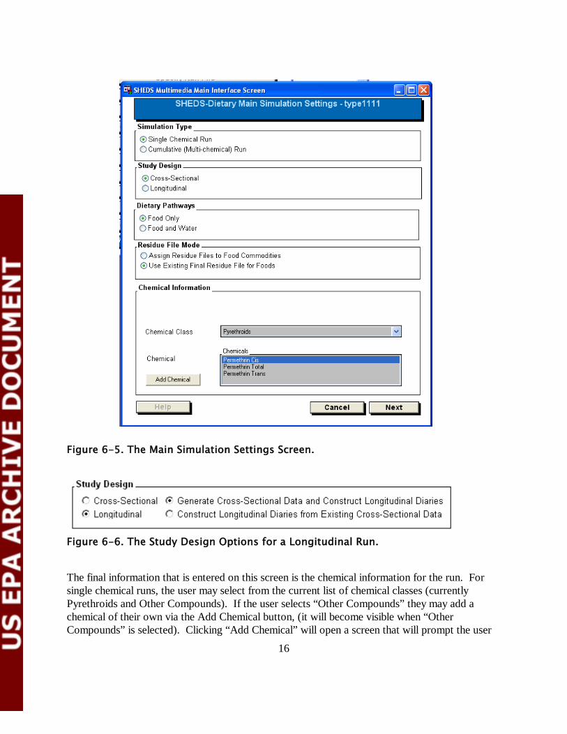
6.4 Main Simulation Settings The first window that a user encounters after creating a new run is the Main Simulation Settings window (Figure 6-5). In this window, the user selects the four main simulation options for performing a SHEDS-Dietary Run: the simulation type (single chemical or cumulative), the study design (cross-sectional or longitudinal), the exposure pathways to model (food exposure or food and water), and an option that determines the type of input residue information the user will be providing. If the user selects “Longitudinal Run,”, then two other options become available in the “Study Design” box (Figure 6-6). The user has the option of creating cross-sectional data and longitudinal diaries at the same time, or constructing longitudinal diaries from existing cross-sectional data (that was created earlier with the model). There are two options for providing residue information in SHEDS-Dietary. In the first option, the user provides individual food residue files (RDF files), which are linked to food commodity groups via the Assign Residues to Foods screen in the interface. The details of this mapping procedure are discussed later in this manual. This option is currently only available for single-chemical cross-sectional runs. The second option is for the user to provide a pre-constructed SAS dataset (a Final or “Processed” Residue File) that contains the residue measurements of interest for different foods. The foods in this file are then linked to food commodity IDs or commodity groups via a mapping file known as a Bridge File. This option is available for any type of run, including cumulative or longitudinal runs. The interface will limit the choices of these options to valid combinations. The contents and formats of all these files are detailed in the Appendix.

16

Figure 6-6. The Study Design Options for a Longitudinal Run.

The final information that is entered on this screen is the chemical information for the run. For single chemical runs, the user may select from the current list of chemical classes (currently Pyrethroids and Other Compounds). If the user selects “Other Compounds” they may add a chemical of their own via the Add Chemical button, (it will become visible when “Other Compounds” is selected). Clicking “Add Chemical” will open a screen that will prompt the user

Figure 6-5. The Main Simulation Settings Screen.

17

to enter a chemical name. When the user selects OK, the chemical will be added to the selection list, which will allow the user to select it. For multiple chemical runs, however, the user must select a Chemical Code file (see Figure 6-7). Chemical Code files contain a list of chemicals that the user may include in the current run. These files are saved in the m_pest library, and their format is described in Section A.2.6. These files can be created in the PDP Generator (see Chapter 6). SHEDS-Dietary contains an example default Chemical Code file for pyrethroids, called b_pestcode. For multiple chemicals, the chemical class is automatically determined by the chemicals contained in the Chemical Code file. If more than one class of chemicals is included in the file, the class will read “Multiple Classes.” Once the desired options and chemicals are selected on the first Main Simulation Settings screen, the user can continue to a second screen of simulation settings. NOTE: This screen is bypassed if the user is creating longitudinal data from an existing cross-sectional run; in this case this input information is not needed since the cross-sectional data has already been generated. However, if the user is generating cross-sectional data and constructing longitudinal diaries, the screen is not bypassed. The appearance of this screen is different depending on the options selected on the first screen; different input settings are required from the user for different types of SHEDS-Dietary runs. The screens for different combinations of the four main settings are shown in Figure 6-8 and Figure 6-9. The settings that the user must potentially select in this window are described below.

Figure 6-7. The Chemical Information Section of the Main Simulation Settings Screen for a Cumulative Simulation.

18

Age Groups. Required for all runs. The user selects the age groups to be considered in the current SHEDS-Dietary run. Multiple groups may be selected. Dietary Data Source. Required for all runs. The source of the dietary food consumption diaries that form the basis of the simulation. The options are diaries from either the Continuing Survey of Food Intakes by Individuals (CSFII) or National Health and Nutrition Examination Survey (NHANES).

Figure 6-8. The Second Main Settings Screen for Single-Chemical Runs.

19

Number of Run Iterations: Required for all runs. This is the number of simulations performed per food diary for all diaries in the selected age group. Multiple runs can be performed to increase the total number of cross-sectional exposure outcomes that are generated. A number of files are also specified in this window. Clicking the button associated with each file opens a selection dialog in the appropriated SHEDS library where the file type is stored. The specific location, contents, and formats of all files are provided in the Appendix. Bridge File: Required for runs using a final (processed) residue file. The main purpose of the Bridge File is to map residue information to different EPA FCID commodity codes. FCID is the Food Commodity Intake Database which refers to food recipes; it is also known as the 100 g tables. Processed Food Residue File: Required for runs using a final (processed) residue file, thus all cumulative runs require this type of file. This file contains a database of residue measurements from different food items, indexed by number (single chemicals) or measured food commodity code (multiple chemicals). The residue measurements from the different food items are linked to specific EPA food commodity IDs via a Bridge File. Processed Water Residue File: Required for all runs modeling water exposure. A file containing water residue measurements is required for all water exposure runs. Processing Factor File: Required for all cumulative runs. If no processing factor data available, then this file can contain values all equal to 1 so that the processing factor will have no effect on the exposure estimates.

20

After the user selects all the settings and files on this screen with valid values, the button on the right of the screen can be selected. In the case of a cross-sectional run, the button will read “Save,” and clicking it returns the user to the main SHEDS screen. When the “Generate Cross-Sectional Data and Construct Longitudinal Diaries” option is being used, the button will read “Next,” and clicking it will send the user to the Longitudinal Settings screen. The Longitudinal Settings screen is the final screen in the Main Simulation Setting screen cascade (Figure 6-10). This screen will appear only for longitudinal runs (i.e. when the longitudinal option was selected on the first main settings screen). It contains the following settings related to creating longitudinal data. Simulation Dates: The start and stop dates for the longitudinal simulation. Diary Assembly Method: SHEDS provides three different methods for assembling longitudinal diaries. The first is an eight-diary method that uses repeats of eight daily diaries for a person (two diaries per season, a weekday and a weekend) to construct the longitudinal diary. The second method is a method that reproduces certain population variance (diversity) and autocorrelation statistics for individuals and the population. The final method uses the results from the cross-sectional analyses – interleaving the outcomes from each person’s two diaries to construct a longitudinal exposure pattern.

Multi-chemical run, food exposure only Multi-chemical run, with water exposure

Figure 6-9. The Second Main Settings Screen for Multi-Chemical (Cumulative) Runs.

21

Key Diary Variable: Only required if the Diversity and Autocorrelation method is selected. This is the variable on the dietary diaries to which the variance-based method is applied. Diversity: Only required if the Diversity and Autocorrelation method is selected. This variable is the desired value of the ratio of between-person variance to total variance in the key diary variable. Autocorrelation: Only required if the Diversity and Autocorrelation method is selected. This variable is the desired value of the ratio of mean day-to-day autocorrelation in the key diary variable.

Prefix for Cross-Sectional Output: All SHEDS output datasets are assigned a prefix. In this manner all datasets from a single run can be identified. If the option “Generate Cross-Sectional Data and Construct Longitudinal Diaries” was selected, this widget will be a text box; the user enters a prefix for the cross-sectional data to be created. If the option “Generate Longitudinal Diaries from Existing Cross-Sectional Data” was selected, this widget will be a selection list of

Figure 6-10. Longitudinal Settings Screen.

22

available cross-sectional runs; the selected prefix will identify the cross-sectional data to be used to create the longitudinal diaries. Longitudinal Dataset Name: This is the name of the dataset where the longitudinal exposure diaries will be stored. Any food exposures are saved in this file, while any water exposures are given the same name, with the added suffix “_w”. The location for longitudinal datasets is the Olong library. Age Groups. The age groups for which to create longitudinal diaries. The displayed age groups will be a subset of those selected for the corresponding cross-sectional run. Number of Persons: The number of persons for which longitudinal diaries will be created. Number of Run Iterations: The number of run iterations to use when constructing the longitudinal diaries. Must be equal to or smaller than the number of runs used to generate the corresponding cross-sectional data. When the option “Construct Longitudinal Runs from Existing Cross-Sectional Data” has been selected, there must be existing cross-sectional data available in the cross-sectional directory, or a message box will appear that reads “Error: No Available Multiple Chemical Cross-Sectional Datasets in Output Library.”

6.5 Import and Enter Residue File

6.5.1 The Residue File Editor and Residue File Format Residue files are text files that contain residue measurements for a particular food group. The measurements define an empirical distribution of residue values from which samples are made. Selecting the “Import and Enter Residue File” button on the Main Screen brings up the Residue File Editor screen (Figure 6-11). This screen can be used to edit existing Residue files or create new files from scratch.

23

Residue files can be created in the SHEDS-Dietary Residue Editor or in any text editor. However, the following formatting rules apply: 1. The file may contain comments; they must be marked with a leading single apostrophe (‘). 2. The file may contain the following descriptive variables, using the keywords below. These variables must be entered each on a line, using the format KEYWORD=value. TOTALNZ - total non-zero residue values in file TOTALZ - total zero residue values LODRES - limit of detection TOTALLOD - total number of limit of detections in file USAGE - pesticide usage percent

AVGPCT - average percent of crop treated MAXPCT - maximum pesticide usage percent

Figure 6-11. The Residue File Editor Screen.

24

3. Of the above keywords, only TOTALNZ and TOTALZ are required by SHEDS to be present. NOTE: Currently, MAXPCT is not used by the model. 4. Residue values may be entered as single numerical values (one on each line) in units of parts per million (ppm). They may also be entered as a block of values using the format NUMBER, RESIDUE where NUMBER is the number of measurements at a particular value, and RESIDUE is the value. Note that NUMBER and RESIDUE must be separated by a comma. The two methods of entering residues (single values and blocks) may both be used in the same file. The total number of measurements (all the single values plus any measurements contained in blocks) must be equal to the TOTALNZ variable (see above). All residue values must be greater than zero. Any zeros should be included in the TOTALZ variable (see above) and not entered as residues. As an example, the following is a valid Residue file: ‘Example Residue File TOTALZ=10 TOTALNZ=20 15, 0.002 0.005 0.005 0.004 0.002 0.006

6.5.2 Importing and Editing a Residue File An existing Residue file can be imported and edited using the Residue File Editor Screen. A file is imported by clicking the “Import Residue File” button. This action opens a standard Windows File selection dialog. The user selects the file to be edited, and then selects “OK”. The values in the residue file are read in to the corresponding widgets on the Residue File Editor. The residue values are loaded into the “Residue and Count Values” text pad. Residue values can be added or edited within this text pad using the formatting rules described above. Any comments in the file (i.e. the lines marked by a leading apostrophe) are displayed in the “Comments” text pad. Comments may be edited or added in this field. The variables listed in the previous section are loaded into the corresponding text boxes along the left side of the Editor. The values for Total Zeros and Total Non-Zeros must be updated to reflect any changes made to the residue values, or else an error will result (see Validating a Residue File, below). The user may elect to save the edited file with the same name by clicking the “Save” button, or save it with a different name using the “Save As” button. Exiting the Editor without saving discards any changes to the Residue file; the user will be prompted to confirm the exit in this case.

25

6.5.3 Creating a New Residue File When the “New Residue File” is clicked, a standard Windows File Selection dialog opens and the user is prompted for a name of the new file. As an alternative, the user may also select an existing Residue file to overwrite. Once the file selection is complete, the user is presented with an entirely blank Editor which can then be populated with residue values, comments, and values for the descriptive variables. The user then proceeds as described above to save the new file when it is complete.

6.5.4 Validating a Residue File Clicking the “Validate” button in the Residue File Editor checks the current values within the Editor (including residue values and the descriptive variables) for errors. Validation is also performed prior to any Save or Save As action. If errors exist, the Editor widget containing the error will be colored yellow, and a description of the error will be printed in the “Validation Errors” text pad. The following are the possible validation errors: • Count of residue values entered does not equal value input to Total Non-Zeros text

box. The correct number of non-zero values will be noted in the Validation text pad. The user must update the Total Non-Zeros text pad to match this value.

• A zero residue value is entered in the text pad. Zero values cannot be added to the list of residue measurements; they must be entered in the Total Zeros text box. For all zero values added to the text pad, the user will be asked if they would like to increment Total Zeros.

• Value too large for percentage. Max Percent Usage and Average Percent Usage must be less than or equal to 100.

• Invalid or negative value. None of the descriptive variables can have negative values.

• Invalid number format. A line with a comma is missing either the residue or count value, or an invalid character or character combination has been entered.

• Error: Fractional counts are not allowed. A non-integer count value is entered on a line with a comma.

• Negative count and residue values are not allowed. A negative count or residue has been entered.

26

6.6 Assign Residues to Commodities The Assign Residues to Commodities screen provides an interactive user interface for assigning residue distribution files (RDF files) to specific food commodities. Residues files may be assigned to a single commodity or to a group of food commodities. In addition, different food forms or cooking methods within a single commodity can be assigned different RDF files, if desired. The food commodities available in SHEDS-Dietary are those listed in EPA's Food Commodity Intake Database (FCID), which was developed from intake commodity data from both CSFII and NHANES-WWEIA.

6.6.1 Overview of the Assign Residues to Commodity Screen Options The Assign Residues to Commodities screen is shown in Figure 6-12 contains a number of widgets to control the quick and intuitive assignment of residue files to commodities. They include:

• Assign Residues by Cooking Status, Cooking Method, or Food Form. These are

three tick boxes under the "Select Options" area. Selecting these options informs the screen that the user intends to assign different residues to commodities based on these food form variables. This controls how many entries per commodity are displayed in the Select One or More Commodities widget (see below). The FCID food form variables specify the commodities’ cooking status (1=cooked, 2=uncooked), food form (1=fresh or not specified; 2=frozen; 3=dried; 4=canned; 5=cured, pickled, smoked, salted; 6=no applicable), and cooking method (0=not specified,1=baked, 2=boiled, 3=fried, 4=fried or baked, 5=boiled or baked).

• Set Residue File Directory. The user can tell the interface where to look for Residue Files by selecting “Set Residue File Directory”. This opens a standard Windows file section dialog. By default, the residue file directory is the folder ./Dietary/rdf under the SHEDS-Dietary main installation directory. Note that currently Residue files must be stored somewhere under the main installation directory tree for SHEDS to run properly. All residue files for a single run must be stored in the same directory.

• Select Crop Group(s). The Select Crop Group(s) widget contains a listing of all the crop groups in the FCID database. The user may select one or more crop groups at a time to assign RDF files. When the user selects a crop group or set of groups, the corresponding commodities are displayed in the Select One or More Commodities widget (see below).

• Select One or More Commodities. This listbox contains a list of all the food commodities for the selected Crop Groups. If the tick boxes for Cooking Status, Cooking

27

Method, and/or Food Forms are selected, then there will be a commodity are entry for each combination of these variables as well, to allow the user to assign residue files specific to these food forms. An example of this is shown Figure 6-13.

Figure 6-12. Assign Residues to Food Commodities Screen.

28

Figure 6-13. The Select One or More Commodities Widget when Food Form Variables (Cooking Method, Cooking Status, and Food Form) are Selected.

6.6.2 Assigning Residues to Commodities The following is the procedure for assigning residue files to commodities:

1) Select the options for assigning residues by cooking status, cooking method, or food form (if desired).

2) Select the location where the residue files are stored. 3) Select the food commodity or commodities (or commodity-food form combinations) to

which to assign residues. 4) Click the "Select Residue File" button. This will bring up a residue file selection box

(Figure 6-14). 5) Select the desired file and click OK. The selected filename will now be shown in the

Residue File text box on the main Assign Residues screen. 6) Click "Apply Data to Selected Commodities" button. This will link the selected file to the

selected commodities. A summary of commodities and their assigned files will be listed in the Defined Commodities table at the bottom of the screen. Each food form available in the FCID database will be individually listed in the summary. Data can be removed from one or more commodities using the "Clear Data from Selected Commodities" button. This will also remove the definitions listed in the Defined Commodities table. The "Clear All" button will remove all data from all commodities.

7) Repeat steps 1-6 for each commodity to be included in the simulation.

29

Figure 6-14. Residue File Selection Box

Note that assigning residue files to all foods in the Bridge File is not required. If a food is not a significant source of the chemical being studied, then it may be ignored. Note: In the future, users will be able to add point residue values to commodities directly in this screen as well. However, currently this can be done by creating a residue file containing a single measurement.

After assigning all the residues, the user can validate the residue information by clicking the "Validate" button if desired (see below). Clicking the "Save and Exit" button will save the Residue-commodity linkage information and return the user to the Main SHEDS screen. The user can return to the Assign Residues screen at any point to edit or add residue assignment information.

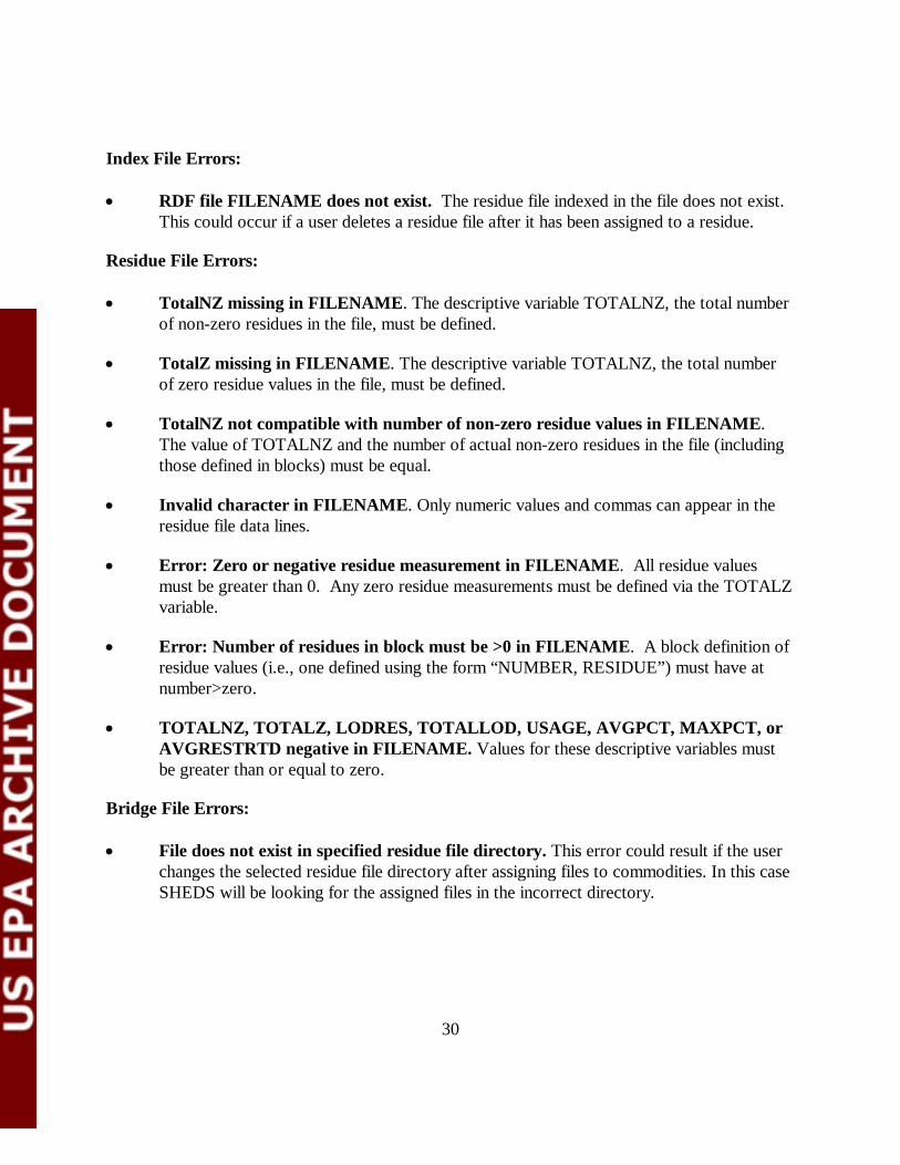
6.6.3 Validating the Residue Data After the residue files have been assigned to commodities, the user can validate the residue information. The validation process will identify any errors in the creation of residue files. Note that the validation procedure that is performed on the Residue Files is the same that is performed on the Residue File Editor screen, but the process is offered here as well since the user may create Residue Files outside of the SHEDS-Dietary editor. The validation process is initiated by clicking the “Validate” button on the Assign Residues to Food Commodities Screen. Any errors are written to the SAS log and to a pop-up error screen (Figure 6-15). The potential errors are given below. Note that the Index File and Bridge File are internal files SHEDS creates. However, errors with these files may indicate an error by the user within the interface.

30

Index File Errors: • RDF file FILENAME does not exist. The residue file indexed in the file does not exist.

This could occur if a user deletes a residue file after it has been assigned to a residue.

Residue File Errors: • TotalNZ missing in FILENAME. The descriptive variable TOTALNZ, the total number

of non-zero residues in the file, must be defined.

• TotalZ missing in FILENAME. The descriptive variable TOTALNZ, the total number of zero residue values in the file, must be defined.

• TotalNZ not compatible with number of non-zero residue values in FILENAME. The value of TOTALNZ and the number of actual non-zero residues in the file (including those defined in blocks) must be equal.

• Invalid character in FILENAME. Only numeric values and commas can appear in the residue file data lines.

• Error: Zero or negative residue measurement in FILENAME. All residue values must be greater than 0. Any zero residue measurements must be defined via the TOTALZ variable.

• Error: Number of residues in block must be >0 in FILENAME. A block definition of residue values (i.e., one defined using the form “NUMBER, RESIDUE”) must have at number>zero.

• TOTALNZ, TOTALZ, LODRES, TOTALLOD, USAGE, AVGPCT, MAXPCT, or AVGRESTRTD negative in FILENAME. Values for these descriptive variables must be greater than or equal to zero.

Bridge File Errors: • File does not exist in specified residue file directory. This error could result if the user

changes the selected residue file directory after assigning files to commodities. In this case SHEDS will be looking for the assigned files in the incorrect directory.

31

Figure 6-15. The SHEDS Error Screen.

32

6.7 Set Up and Run SHEDS-Dietary Module Selecting “Set Up and Run SHEDS-Dietary Module” from the Main Screen opens the Run Screen (Figure 6-16). This screen is used to set a number of options for the current SHEDS-Dietary run, which are then saved in the Run file. This screen is also used to initiate the actual SHEDS-Dietary simulation. In this screen, the user can both confirm settings that have already been selected for the run, and set risk parameters and other options. The appearance of this screen is also dependent on the run settings. All of the required files designated in the Main Settings Screen can also be updated here prior to running the simulation. The types of files that are present depend on the run type. In the case of a run where the “Convert Via Bridge File” option is used, the residue file location (directory) is present. The selection widgets for these files will be pre-populated with the values chosen earlier; this screen gives the user a chance to make any final changes.

Single Chemical Multichemical

Figure 6-16. The Run SHEDS-Dietary Screen for Single and Multichemical Cross-Sectional Runs

33

In addition, the output file libraries and prefixes for cross-sectional and (if present) longitudinal data are also present in the Output Settings box on the screen. A note about prefixes: if the prefix designated does not end with an underscore, SHEDS will add one. This underscore is necessary for constructing the filenames. When the user visits the screen again, the underscore will be present. Again, these values are populated with any prior selections of these values that were made on the Longitudinal Settings screen. In the case of a solely cross-sectional run, the output library and prefix are first specified here. The user may also indicate which outputs should be written for the run using three checkboxes: Daily Totals and/or Eating Occasions.

6.7.1 Other Options There are three additional options provided in this section. • Use Pesticide Usage to Fill in LOD for No Detected Value. Use any pesticide usage

information included in the residue files to fill in limit-of-detection values. • Bayer DWCS. Use data from the Bayer Drinking Water Consumption Survey (Barraj

and Daniels, 2004) to model direct drinking water consumption (the default). If this box is unchecked, CSFII data will be used to model water consumption (spread equally over 6 drinking occasions per day).

• Same Food-Same Residue. When this option is selected, any instance of the same RAC

of the same food being eaten more than one time in day will use the same sampled value from the residue distribution.

6.7.2 Risk (Toxicological) Parameters Risk (toxicological) parameters are also entered on the Set Up and Run screen. NOTE: Currently these risk factors are not used by the model, therefore risk values have not been linked with exposure values in this version. The parameters are given in Table 6-1. By default, all risk (toxicological) parameters are initially given a value of 0.002.

34

Table 6-1. Risk (Toxicological) Parameters in the Run Information File

Risk (Toxicological) Parameter Description aRFD Acute reference dose aRDF: Default Default acute reference dose Chronic PAD: Default Chronic population adjusted dose Chronic PAD: Females 13-49 Chronic population adjusted dose for females

13-49 Acute PAD: Default Default acute population adjusted dose for

females 13-49 Acute PAD: Females 13-49 Acute population adjusted dose for females 13-

49 Chronic NOEL Chronic no observed effect level Acute NOEL Acute no observed effect level Cancer Q Cancer potency factor Reference dose is assigned to each age group; the user must select each defined age group from the Age Group menu and enter appropriate values for the parameter. If an invalid value has been assigned for any age group, the field will be colored yellow, indicating an error. Note that this may occur, even if the value for the currently displayed age group is valid. If an error exists, a text field will appear at the bottom of the Run Screen and the current errors will be displayed (Figure 6-17). All errors in this field need to be resolved before the user can save the Run File or run the SHEDS-Dietary simulation.

Figure 6-17. Run Screen Error Field

Advanced users of SHEDS-Dietary may want to directly view or edit values of the Run Files variables. This can be done using the Check Run Variables screen (Figure 6-18), which is initiated via the “Check Other Inputs” button on the Set up and Run screen. This screen will display all the relevant Run File variables for the current run, editable as text. Note that any changes made to the Run File from this dialog is not subjected to the rigorous error testing that is provided by the other interface screens. When all the fields in the run screen are completed with valid values, then the “Save Run File”, “Save As Run File” and “Run Simulation” buttons are active. Clicking the Save Run File button

35

will save all the current values of the Run file variables. The Save As Run File button performs the same function as the Save Run File button, with the exception that is always opens a dialog in order for the user to designate a filename different from the current Run file name. Finally, selecting the “Run Simulation” button will initiate the SHEDS-Dietary Run. The model outputs are discussed in Appendix A of this manual.

Figure 6-18. Check Run Variables

6.8 Pre-Process Output Data Once cross-sectional data is generated by a SHEDS-Dietary run, it must be processed to generate summary and percentile data tables. The contents of these tables are described in the Appendix. This step is accomplished via the Pre-Process Output Data screen (Figure 6-19), which is accessed via a button on the Main SHEDS Screen. If the user has a Run File open when the screen is initiated, much of the data in this screen will be populated with valid values. The user may also open a new Run File via the Runinfo file button at the top of the screen.

36

The following variables must be specified in this window in order to successfully preprocess cross-sectional output data. Input Data Library: This is the library where the data that is to pre-processed (the cross-sectional model output) is located. Selecting a library will populate the Input Data Prefix widget with a list of the available cross-sectional runs. Input Data Prefix: The user selects the prefix of the model output data they would like to preprocess from the list. (Recall that all model runs are supplied a output prefix for identifying unique sets of data). This selection will populate several of the other widgets on the screen with default values. Output data Library: This is the library where the SHEDS summary datasets will be created. By default, the data is written to the Sumtab library, but the user may select any library.

Figure 6-19. The Preprocess Output Data Screen.

37

Output Data Prefix. This is the prefix for the output data table filenames. The interface will add a underscore to all prefixes before they are used to create filenames. Input Variable: The variable to be processed. In a single chemical run, this variable is always called “Exposure: XXX” where XXX is a chemical name. In a multi-chemical run, the variables will be identified as either “Total Exposure” (total cumulative exposure) or Exposure: XXX, where XX X is a chemical name. Use Half-Life. If this option is selected, SHEDS uses a half-life value (in hours) when estimating exposures, otherwise, SHEDS uses the Maximum Exposure-Eating Occasion to calculate per capita exposures. Input Variable Label. Label to give the input variable in the processed datasets. (Not currently required). Loop Number: Number of run iterations (loops) to include in the summary statistics. For example, if 4 repetitions were run in the original simulation, the user may choose any number less than 4 to include in the summary statistics. Contribution for Lower Percentile and Contribution for Upper Percentile. Specify lower and upper range for contribution analyses. Pathway. Pathways to include in the analysis. Label. Label for the output datasets. (Not currently required).

38

6.9 View Results Selecting the “View Results” button on the Main SHEDS-Dietary screen opens the View Results window (Figure 6-20), which contains two option buttons: View Cross-Sectional Results and View Longitudinal results. Clicking either of these buttons will open a screen to that provides to the user tools for viewing and exploring the results of the current SHEDS-Dietary run or previous runs. Details of the View Results windows are discussed in the next two sections.

6.9.1 The View Cross-Sectional Results Window The View Cross-Sectional Results window is used to view the summary datasets that are generated using the Pre-process output screen. This screen has two sections, the control section and the display window. The control section (Figure 6-21) contains the widgets and menus that control the creation of the tables and figures. The display window is directly beneath the control section; it is the area of the screen where the selected figure or table is displayed. After the user selects the desired settings from the control section, he or she can select the “Update Display” button to render the figure or table in the display window. Selecting the “Print the Figure” button sends whatever figure or table is currently displayed to the default printer. There are several widgets and menus that are used to select the figure or table to display. The “Set Output Library” button is used to designate which SAS library contains the output data of interest. By default, this is the main SHEDS-Dietary library named “output.” Clicking this button will bring up a SAS library dialog box, in which the user may select other available SAS libraries, if desired.

Figure 6-20. The View Results Screen.

39

Figure 6-21. The View Cross-Sectional Results Control Section

The “Select Run to View” menu will be populated with a list of all of the runs whose outputs are saved in the current run library. By default, the first run in the list will be selected. As is normal in SHEDS, the output is selected by choosing the prefix for the run of interest. The “Select Output to View” menu provides 5 different methods of visualizing the results of a model run. These output types are: • CDFs. Plot cumulative distribution functions for one or more exposure or dose variables.

• Exposure: Percentile Table. Display a table containing selected population statistics for one or more exposure variables.

• Exposure and %APAD: Summary Table. Display a table containing percentiles and statistics for both exposure and % APAD.

• Contribution by Commodity: Bar or Pie Chart. Plot the contribution of each food commodity to either the amount of food or chemical consumed, either in bar or pie chart format.

• Contribution by Commodity: Summary Table. Display a table listing the contribution of each food commodity to either the amount of food or chemical consumed.

These output types are defined in detail (with examples) in the next five subsections. For each of the above output types, the population group of interest must be set using the Select Population Group Menu. The population groups available are only those that were included in the run. If either Exposure: Percentile Table and Exposure and %APAD: Summary Table is

40

selected as the output to view, there will an All Groups option available and the resulting table will include entries for all of the population groups in the run. All the other output types can only display one population group at a time. The last two menus in the control section of the screen are the Variable Group and Select Variable(s) menus. These control which variables are displayed on the current figure or table. The contents of these menus will differ for each output type; they are discussed below. When viewing a figure, a “Print Figure” button will be visible. Clicking this button will print a copy of the current figure to the default printer. When viewing a table, a “Print to File” button is visible. This button can be used to save the current table in *.csv format. The table can also be printed to the default printer by right-clicking on the table and selecting “Print.”

6.9.2 CDFs By selecting the CDFs option on the Select Output to View menu the user can plot cumulative distribution functions of exposure and dose variables. Multiple CDFs (exposure or dose variables) can be displayed at one time. The user first selects either Exposure or Percent Acute Population Adjusted Dose from the Variable Group menu. This selection will populate the Select Variable(s) menu with either a list of exposure or %APAD variables. For exposure, the available variables are: • Dietary Exposure: Day • Water Exposure: Day • Combined Exposure: Day • Dietary Exposure: Eating Occasion • Water Exposure: Eating Occasion • Combined Exposure: Eating Occasion For % APAD, the available variables are: • Dietary % APAD: Day • Water % APAD: Day • Combined % APAD: Day • Dietary % APAD: Eating Occasion • Water % APAD: Eating Occasion • Combined % APAD: Eating Occasion

41

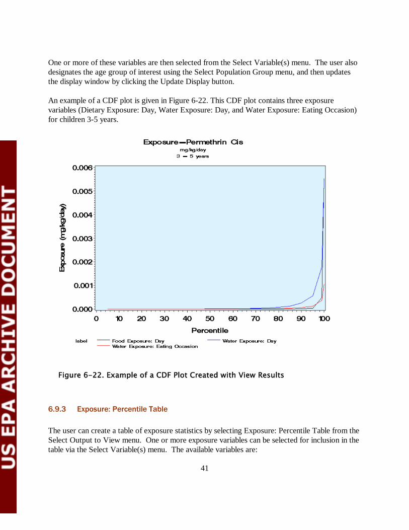
One or more of these variables are then selected from the Select Variable(s) menu. The user also designates the age group of interest using the Select Population Group menu, and then updates the display window by clicking the Update Display button. An example of a CDF plot is given in Figure 6-22. This CDF plot contains three exposure variables (Dietary Exposure: Day, Water Exposure: Day, and Water Exposure: Eating Occasion) for children 3-5 years.

6.9.3 Exposure: Percentile Table The user can create a table of exposure statistics by selecting Exposure: Percentile Table from the Select Output to View menu. One or more exposure variables can be selected for inclusion in the table via the Select Variable(s) menu. The available variables are:

Figure 6-22. Example of a CDF Plot Created with View Results

42

• Dietary Exposure: Day • Water Exposure: Day • Combined Exposure: Day • Dietary Exposure: Eating Occasion • Water Exposure: Eating Occasion • Combined Exposure: Eating Occasion One or more of these variables are then selected from the Select Variable(s) menu. The user also designates the age group of interest using the Select Population Group menu. For this output type, the user can choose to include all available population groups in the table by selecting All Groups from the menu. The table is created by clicking the Update Display button. This type of output table includes the following information (columns): • Exposure Type: Food (Dietary), Water, or Combined • Exposure Category: Daily or Eating Occasion • Age Group: One or more Population age groups as defined using the Select Population

Group menu • Sample size: number of simulated persons in age group (number of person days = number

of daily food diaries times the number of run iterations) • Mean, Standard Deviation, Median, and 5th, 25th, 75th, 95th and 99th percentiles: statistics

of the corresponding exposure variable for age group An example of an exposure percentile table is given in Figure 6-23. In this example, daily food (dietary) and water exposures are given for all population groups.

Figure 6-23. Example of an Exposure Percentile Table

43

6.9.4 Exposure and aPAD: Summary Table

The user can create a summary table of exposure and dose (%APAD) statistics by selecting Exposure and aPAD: Summary Table from the Select Output to View menu. One or more exposure variables (and the corresponding doses) can be selected for inclusion in the table via the Select Variable(s) menu. The available variables are: • Dietary Exposure: Day • Water Exposure: Day • Combined Exposure: Day • Dietary Exposure: Eating Occasion • Water Exposure: Eating Occasion • Combined Exposure: Eating Occasion One or more of these variables are then selected from the Select Variable(s) menu. The user also designates the age group of interest using the Select Population Group menu. For this output type, the user can choose to include all available population groups in the table by selecting All Groups from the menu. The table is created by clicking the Update Display button. The Exposure and APAD Summary Table includes the following information (columns): • Exposure Type: Food (Dietary), Water, or Combined • Exposure Category: Daily or Eating Occasion • Age Group: One or more Population groups as defined using the Select Population Group

menu • Sample Size: number of simulated persons in age group • The 95th , 99th, and 99.9th percentiles An example of an exposure and APAD Summary Table is given in Figure 6-24. In this example, daily combined exposures are given for all population groups.

Figure 6-24. Example of an Exposure and %APAD Summary Table

44

6.9.5 Contribution by Commodity: Bar Chart or Pie Chart By selecting the Contribution by Commodity: Bar Chart or the Contribution by Commodity: Pie Chart option on the Select Output to View menu the user can create plots of the contribution of individual food commodities to exposure. The user selects the desired variable from the Select Variable(s) menu. The available variables are: • % Food: For each food commodity, the percent of total food consumed. • % Chemical: For each food commodity, the percent of total chemical consumed. Only commodities accounting for greater than 1% of the total food or chemical consumed are included in the graphs. The user selects one of these variables, and then designates the age group of interest using the Select Population Group menu. The chart is created in the display window by clicking the Update Display. An example of a Contribution by Commodity Bar Chart is given in Figure 6-25. In this example, the age group of interest was children aged 3-5 years. An analogous pie chart for children 0-1 years is given in Figure 6-26.

45

Figure 6-25. Example of a Contribution by Commodity Bar Chart

46

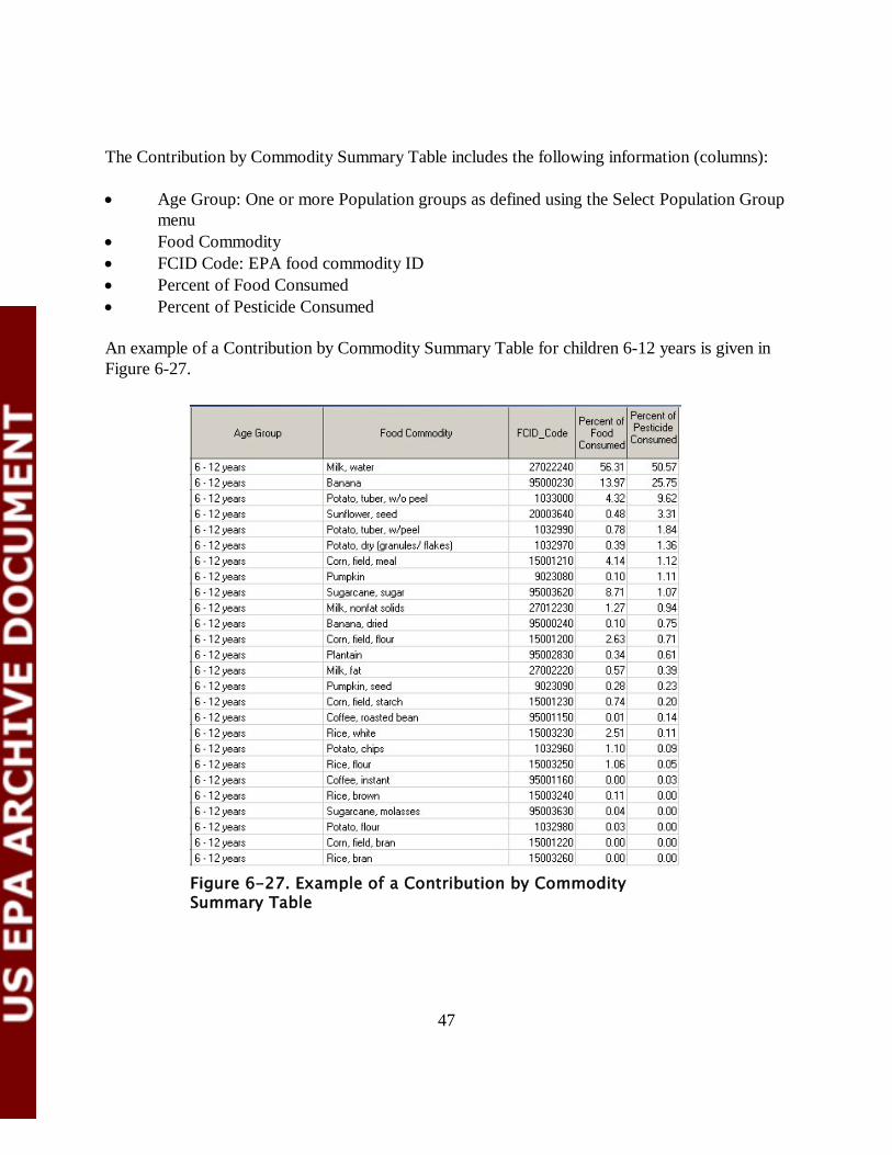
6.9.6 Contribution by Commodity: Summary Table The user can create a summary table contribution by commodity statistics by Contribution by Commodity: Summary Table from the Select Output to View menu. For this output type there are no variables to select; information on both the percent of food and chemical consumed are included automatically in the table.

Figure 6-26. Example of a Contribution by Commodity Pie Chart

47

The Contribution by Commodity Summary Table includes the following information (columns): • Age Group: One or more Population groups as defined using the Select Population Group

menu • Food Commodity • FCID Code: EPA food commodity ID • Percent of Food Consumed • Percent of Pesticide Consumed An example of a Contribution by Commodity Summary Table for children 6-12 years is given in Figure 6-27.

Figure 6-27. Example of a Contribution by Commodity Summary Table

48

6.9.7 View Longitudinal Results The longitudinal time series of daily exposures can be visualized using the View Longitudinal Results window. The View Longitudinal Results window (Figure 6-28) is similar in format to the cross-sectional window, in that it contains a control section and a display window. As discussed before, the user may select both an output data library (by default, the Olong library) and a run to view. The variable selection list is populated with the available exposure variables for the loaded run. For a single chemical run, food (dietary) exposure and water exposure (if present) are available. For a cumulative run, food (dietary) and water exposures for each chemical as well as total exposures will be present in the selection list. The user can limit the portion of the simulation to be viewed by selecting a start and ending date. Each person in the run is listed in the Select Individuals list box. The user can choose a single individual to view by clicking on a single person ID, or view multiple individuals by clicking and dragging within the list box.

An example of a daily exposure time series is shown in Figure 6-29.

Figure 6-28. The Control Section of the View Longitudinal Results Window

49

Figure 6-29. A Daily Exposure Time-Series for a Longitudinal Run.

If the “Use Half-Life” button is selected, the time-series of persistent exposure is also plotted on the graph. The user enters a half-life (in hours) and clicks the Update Display button. The persistent exposure will be added to the plot. An example for cis-permethrin using a half-life of 48 hours is shown in Figure 6-30.

50

Figure 6-30. A Persistent Exposure Time Series Added to a Longitudinal Plot.

51

7 PDP Generator The PDP Generator is a feature that allows the user to create multichemical input files for SHEDS-Dietary using data from the U.S. Department of Agriculture’s Pesticide Data Program database. This database contains food residue measurements collected from 1996-present for dozens of chemicals. See the SHEDS-Dietary Technical Manual (Xue et al., 2010) for more information about the PDP database and the information it contains. The PDP Generator screen is shown in Figure 7-1. The user first selects one or more chemical classes from the Select Chemical Classes to View list box. The chemicals available in the database in these classes are then listed in the Available Chemicals list box. The user then highlights one or more chemicals in the list box and uses the arrow keys to move them to the Chemicals to Use list. NOTE: Although the PDP Generator creates input files for cumulative (multi-chemical) runs, it is a valid choice in SHEDS-Dietary to perform runs in cumulative mode that contain a single chemical. Therefore, creating files with only one chemical is valid.

Figure 7-1. The PDP Generator Screen.

52

Once the list of chemicals to use is created, the user must then select names and locations for the three output files that the PDP generator creates: 1. A Chemical Code file. Chemical code files are discussed in Section 6.4 and Appendix A. By default, the code file is saved in the default SHEDS-Dietary multichemical chemical code library (m_pest). 2. A Residue file. Multichemical residue files are discussed in Section A.2.3. By default, the residue file is saved in the default SHEDS-Dietary multichemical residue library (m_res). 3. A Processing Factor file. Processing Factor files are discussed in Section A.2.5. By default, the residue file is saved in the default SHEDS-Dietary multichemical processing factor library (m_pf). These files can then be used as input to future SHEDS-Dietary runs. When a multichemical run is created using these files, the user will also need to designate a bridge file. The bridge file B_py_bridge (that is included with the SHEDS-Dietary release) may always be used with files created with the PDP Generator. WARNING: When using these files in a run, these three files must all be used together. These files may not be compatible with other files generated outside of SHEDS or made with different PDP generator settings. Therefore, it is a good idea to name them in such a way (with a prefix, for example) that makes it easy to recall which files are compatible.

53

8 Example Case Studies The following case studies are meant to guide the user completely through multiple examples of running SHEDS-Dietary from start to finish. Each step in the examples are described briefly, and illustrated with accompanying screenshots. Any necessary input files are included with SHEDS-Dietary or created within the case study steps. The main run options for the included case studies included are as follows: Case Study 1: Arsenic (As). Single chemical, cross-sectional run. Food exposure only. Convert food residue files via Bridge File. This case study resides in the SHEDS Quick Start Guide. Case Study 2: Cis-Permethrin. Single chemical, cross-sectional run. Food exposure only. Use final residue file. Case Study 3: Cis-Permethrin. Single chemical, longitudinal run. Food exposure only. Use final residue file. Case Study 4: Pyrethroids. Multi-chemical, cumulative, cross-sectional run, using input files made with the PDP Generator. Food exposure only. Use final residue file.

8.1 Case Study 2: Cis-Permethrin, Cross-Sectional Run This case study is a single-chemical example for simulation of food exposure to cis-permethrin. This is also a cross-sectional simulation. This run uses a final residue file, rather than assigning residue files to commodities. 1) Create the Bridge File and final residue files for the chemical. This method is best used by

persons familiar with the creation or editing of SAS datasets. The format of these files is described in the Appendix. In addition, the SHEDS installation provides several examples of these files that can be used as templates. A final residue file final_cisperm_res and Bridge File I_perm_cisbridge were generated. These files are included in the SHEDS-Dietary installation; they will be available for selection as the user steps through this case study.

54

Final (processed) residue file, final_cisperm_res

Bridge file, I_perm_cisbridge

55

2) Initiate a SHEDS-Dietary session by double-clicking the SAS icon.

Double click here to start SAS

3) Select <Specify Run File>-><Create New Run File> to initiate the creation of a new run for cis-permethrin. Follow the steps provided in the Case Study in the Quick Start Guide to specify a new run called "Cispermethrin."

4) The Main Simulation Settings button will now be enabled. Select it and the Main Simulation Settings screen will appear. Select “Pyrethroids” for Chemical Class in the Chemical Information box and Permethrin Cis for pesticide. Select “Use Existing Final Residue File for Foods” in the Residue File Mode box (note that this option is different from that used in Case Study #1), then hit the Next button.

56

Select <Main Simulation Settings>

57

5) The second Main Simulation Settings screen appears. Click the Bridge File button to select a Bridge File for the run. Select I_perm_cisbridge from the file selection dialog, then hit OK. The dialog widget will be filled in with the full name of the dataset (including the SAS library). For the Processed Food Residue File, select the file Final_cisperm_res from the selection dialog. Then select 3 as the number of run iterations and click <Save>.

Select bridge file and final residue files, click <Save> 6) Select the <Set Up and Run SHEDS-Dietary> button from the Main SHEDS screen. This

screen finalizes the settings for the run. Specify an Output File Prefix for the run (“cisperm_”). Edit any desired risk (toxicological) parameters (or use the ones provided in the example). The simulation is then run by selecting <Run Simulation>, then hit <Exit>. When the run is complete, click <Close>.

58

59

7) Now preprocess the raw model output data to generate summary tables and percentiles that

can be visualized (the screen will open automatically when the Run Progress screen is closed). Select the prefix of the run to be preprocessed (“cisperm_”) and a prefix for the summary data (“cispermsum”). Select the variable to process. Since this is a single chemical run, the only available variable is Exposure: Permethrin Cis. Also select how many run iterations should be processed and the contribution percentiles. Click <Run Preprocessing Routine>, then <OK>.

Enter a prefix for the summary data (“cispermsum”) and click <Run Preprocessing Routine>. 8) Click on the <View Results> button to display the View Results selection screen. Select

<View Cross-Sectional Results>.

60

Click here

9) The main View Cross-Sectional Results screen will now appear. Select the run of interest from the run selection list, by selecting the prefix that was entered in the Pre-process screen (cispermsum, in this case). Select “CDFs” as the output to view, and highlight one of the two available variables (daily or eating occasion food exposure). Selecting <Update Display> will

61

update the figure with the selected options. In this way, different output tables and graphs can be generated.

Select the run “cispermsum”, “CDFs” as output to view, and <Update Display> 10) Select “Exposure Percentile Table” as the output to view, select the two available variables,

and click <Update Display>. This will generate the requested table for the selected variables.

62

11) Repeat this process by selecting “Exposure and %APAD: Summary Table” and again

updating the display.

12) Selecting “Contribution by Commodity: Bar Chart” as output to view and %Chemical as the

variable produces a bar chart of the contribution of food types to total chemical exposure.

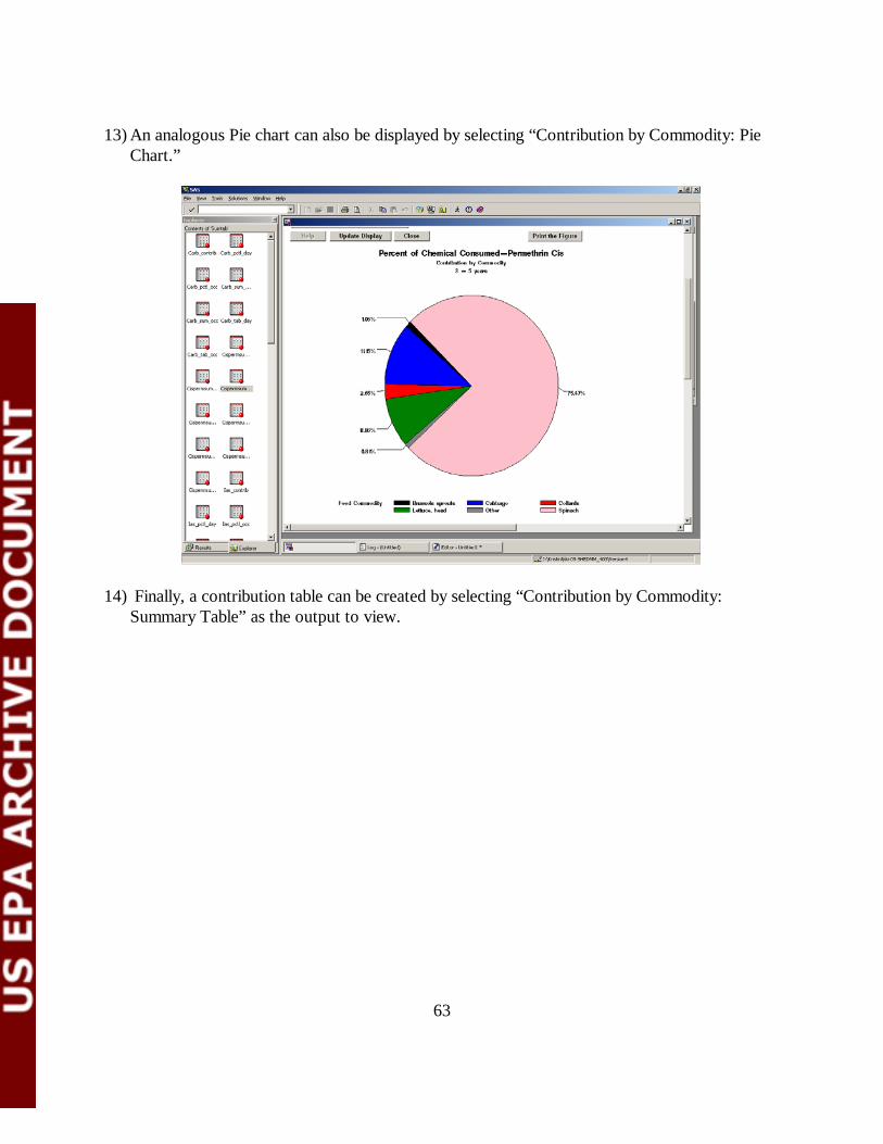
63

13) An analogous Pie chart can also be displayed by selecting “Contribution by Commodity: Pie Chart.”

14) Finally, a contribution table can be created by selecting “Contribution by Commodity: Summary Table” as the output to view.

64

65

8.2 Case Study 3: Cis-Permethrin, Longitudinal Run This case study is a single-chemical example for simulation of food exposure to cis-permethrin. This is a longitudinal, rather than cross-sectional, simulation. This run also uses a final residue file, rather than converting food residue files. Steps 1)-5). Repeat Steps 1-5 of Case Study 2, giving the run the name “Cisperm”.

6) The Main Simulation Settings button will now be enabled. Select it and the Main Simulation Settings screen will appear. Select “Pyrethroids” for chemical category and Permethrin Cis for chemical. Select “Longitudinal” under the Study Design box, then hit <Next>.

Select <Longitudinal> and <Permethrin Cis>

7) The second Main Simulation Settings screen appears. Click the Bridge File button to select a Bridge File for the run. Select I_perm_cisbridge from the file selection dialog, then <OK>. For Processed Food Residue file, select the file final_cisperm_res from the selection dialog. (The text field will be filled in automatically with the full name of the dataset, including the SAS library prefix). Then select 3 as the number of run iterations and click <Next>.

66

Select bridge file and final residue file, click next 8) The Longitudinal dataset screen now opens. Select 1-1-2006 as the start date of the run and 12-31-2006 as the end date. The dates can be entered as text in the fields or selected using the arrow buttons. Select “Diversity and Autocorrelation” as the Diary Assembly Method. Enter 0.3 for both the Diversity and Autocorrelation values. Enter “cperm_” as the prefix for the cross-sectional output data, and “cperm_long” as the name of the longitudinal dataset file. Choose to simulate 100 people. Select 3 as the number of cross-sectional run iterations to include when creating the longitudinal exposures, then hit <Save>.

67

Select <Diversity and Autocorrelation method. Enter diversity and autocorrelation values. Select run dates, names for output files, number of persons, number of interaction runs to use, and. Click <Save>.

9) Select the <Set Up and Run SHEDS-Dietary> button from the Main SHEDS screen. This screen finalizes the settings for the run. Edit any of the example risk parameters as desired. The simulation is then run by selecting <Run Simulation>. Depending on computing resources, this may take more than several minutes. When completed, hit <Exit.>

68

Click here

Accept defaults, and click <Run Simulation>

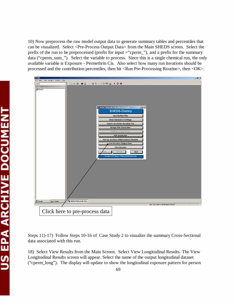
69

10) Now preprocess the raw model output data to generate summary tables and percentiles that can be visualized. Select <Pre-Process Output Data> from the Main SHEDS screen. Select the prefix of the run to be preprocessed (prefix for input =“cperm_”), and a prefix for the summary data (“cperm_sum_”). Select the variable to process. Since this is a single chemical run, the only available variable is Exposure - Permethrin Cis. Also select how many run iterations should be processed and the contribution percentiles, then hit <Run Pre-Processing Routine>, then <OK>.

Click here to pre-process data

Steps 11)-17) Follow Steps 10-16 of Case Study 2 to visualize the summary Cross-Sectional data associated with this run. 18) Select View Results from the Main Screen. Select View Longitudinal Results. The View Longitudinal Results screen will appear. Select the name of the output longitudinal dataset (“cperm_long”). The display will update to show the longitudinal exposure pattern for person

70

number 1. Any person from the simulation can be viewed, by using the “Select Individuals” list box. Multiple persons can be visualized at once by clicking and dragging on the selection box to highlight multiple persons, and then clicking “Update Display.” The persistence of the chemical in the body can also be added to the plot, by checking “use-half life”, entering a half-life value (hit the return button), and clicking “Update Display”. The example below depicts the results of using a half-life of 48 hours. NOTE: Time series may not look identical to that shown below due to the stochastic nature of the longitudinal diary assembly.

Click here

71

72

73

8.3 Case Study 4: Pyrethroids, Cross-Sectional Run This case study is a cumulative (multi-chemical) example for simulation of food exposure. This is a cross-sectional simulation. This run uses files created by the PDP Generator. 1) Proceed to SHEDS as in the above demos.

2) Select the PDP Generator.

Click <PDP Generator>

3) Select the chemical class “Pyrethroids”. (Note that additional classes can also be viewed by clicking on the class name). For this example, click and drag in the Available Chemicals list box to highlight “Bifenthrin”, Cyfluthrin”, “Cypermethrin”, and “Permethrin Total.” Click the single arrow button to select these chemicals. They will move to the Chemicals to Use listbox. Enter names for the Chemical code file, the residue file, and the processing factor file: py_pest, py_res, and py_pf. Click “Create Data Files”. (This may take several minutes). When the screen closes, the file creation is complete.

74

Click and drag to highlight the first four chemicals

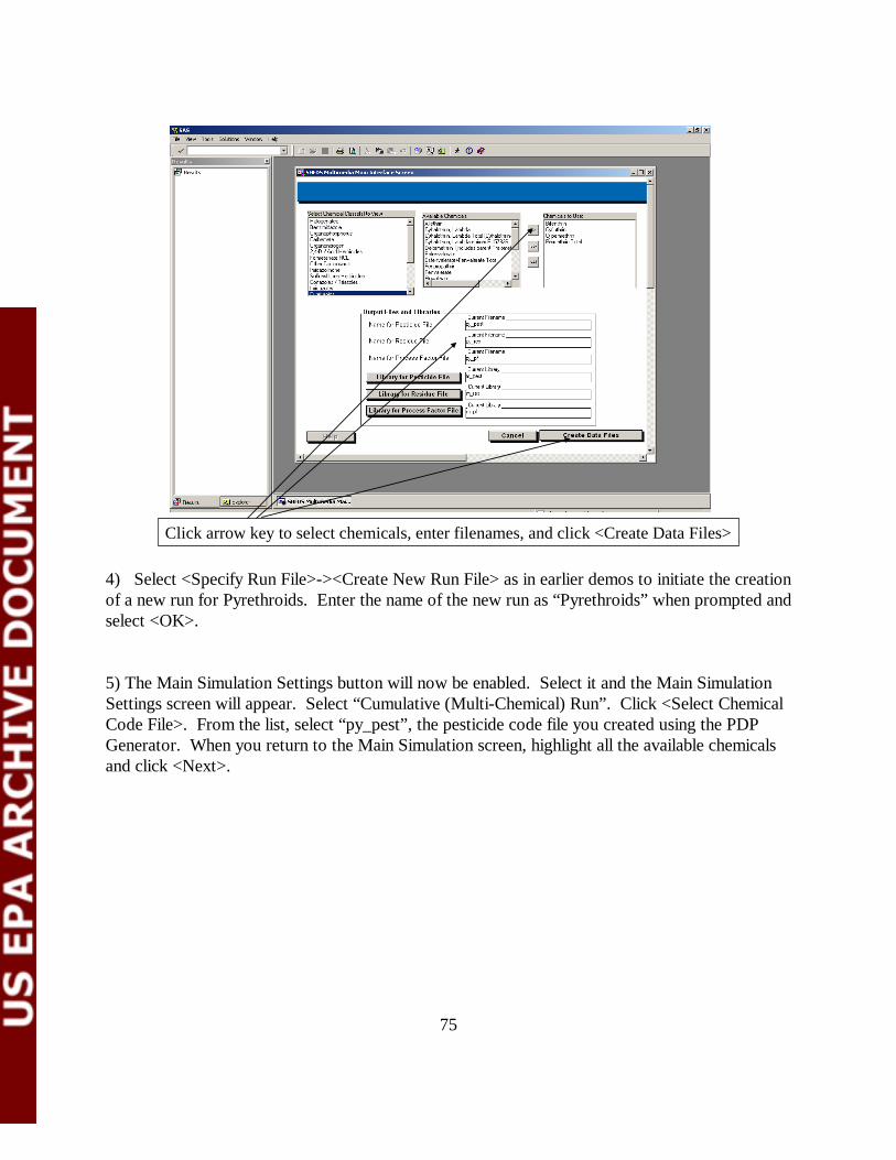
75

Click arrow key to select chemicals, enter filenames, and click <Create Data Files> 4) Select <Specify Run File>-><Create New Run File> as in earlier demos to initiate the creation of a new run for Pyrethroids. Enter the name of the new run as “Pyrethroids” when prompted and select <OK>.

5) The Main Simulation Settings button will now be enabled. Select it and the Main Simulation Settings screen will appear. Select “Cumulative (Multi-Chemical) Run”. Click <Select Chemical Code File>. From the list, select “py_pest”, the pesticide code file you created using the PDP Generator. When you return to the Main Simulation screen, highlight all the available chemicals and click <Next>.

76

Select <Cumulative Run> and click <Select Chemical Code File>

Select file “Py_pest” and click <OK>.

77

Select all four chemicals, click <Next>

6) The second Main Simulation Settings screen appears. Click the Bridge File button to select a Bridge File for the run. Select B_py_Bridge from the file selection dialog. Repeat the process to select the processing factor and dietary residue files, selecting “py_pf” and “py_res” (text fields will fill in with the full dataset name, including the SAS library prefix) . Then select 1 as the number of run iterations and click <Save>.

78

Click <Bridge File>, select “B_py_bridge’ from dialog. Repeat for Processing factor and Dietary residue files, selecting “py_pf” and “py_res,”respectively. Click <Save>.

7) Select the <Set Up and Run SHEDS-Dietary> button from the Main SHEDS screen. This screen finalizes the settings for the run. Provide a prefix for the run (“py_test_”). Edit any desired risk (toxicological) parameters. The simulation is then run by selecting <Run Simulation>.

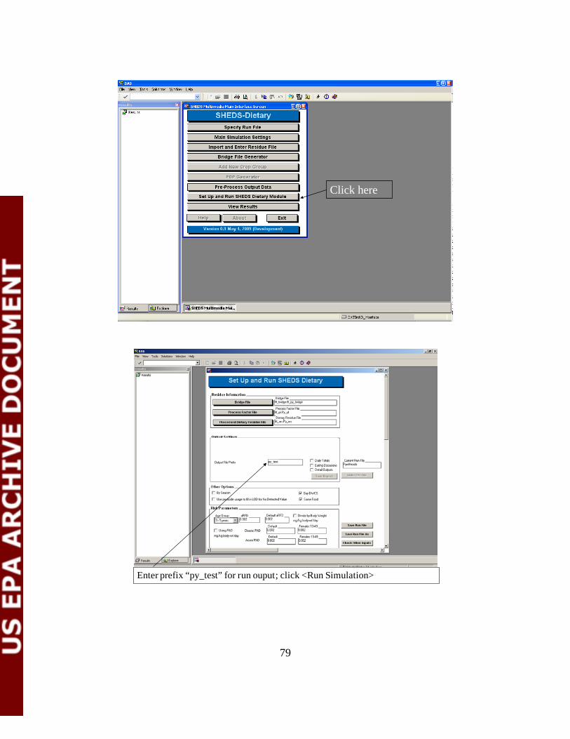
79

Click here

Enter prefix “py_test” for run ouput; click <Run Simulation>

py_test

80

8) The "Preprocess Output Data" screen will open automatically upon exiting the Run screen. Select the prefix of the run to be preprocessed (“py_test_”), and a prefix for the output (“total_exp_”). Select the variable to process. Since this is a multiple chemical run, exposure variables for many different chemicals are available. Select “Total Exposure”, which the cumulative exposure due to the four selected chemicals for the run. Also select how many run iterations runs should be processed and the contribution percentiles.

9) Click on the <View Results> button to display the View Results selection screen. Select <View Cross-Sectional Data>.

10) The main View Cross-Sectional Results screen will now appear. Select the run of interest from the run selection list, by selecting the prefix that was entered in the Pre-process screen (“total_exp”, in this case). Select “CDFs” as the output to view, and highlight one of the two available variables (daily or eating occasion food exposure). Selecting <Update Display> will update the figure with the selected options. In this way, different output tables and graphs can be generated.

Select “TOTAL_EXP” from list. Click <Update Display>.

81

11) Select “Exposure Percentile Table” as the output to view, and click <Update Display>. This will generate the requested table for the selected variables.

Select “Exposure: Percentile Table” from list. Click <Update Display>.

Select “Exposure: Percentile Table” from list. Click <Update Display>.

82

12) Repeat this process by selecting “Exposure and %APAD: Summary Table” and again updating the display.

Select “Exposure and %APAD: Summary Table” from list. Click <Update Display>.

83

13) Selecting “Contribution by Commodity: Bar Chart” as output to view and “%Chemical” as the variable produces a bar chart of the contribution of food types to total chemical exposure.

Select “Contribution By Commodity: Bar Chart” from list and %Chemical as the variable. Click <Update Display>.

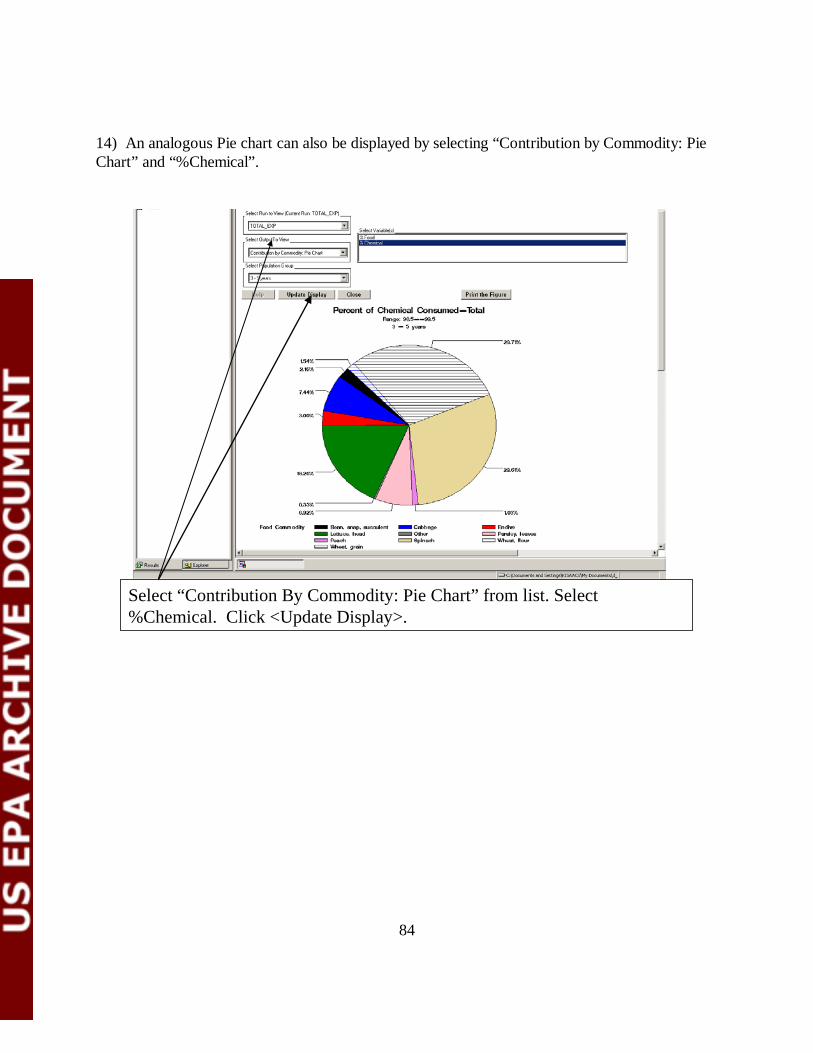
84

14) An analogous Pie chart can also be displayed by selecting “Contribution by Commodity: Pie Chart” and “%Chemical”.

Select “Contribution By Commodity: Pie Chart” from list. Select %Chemical. Click <Update Display>.

85

15) Finally, a contribution table can be created by selecting “Contribution by Commodity: Summary Table” as the output to view.

Select “Contribution By Commodity: Summary Table” from list. Click <Update Display>.

86

9 References Barraj, L.M., Daniels, C.L. 2004. “Drinking Water Consumption Survey”, September 15, 2004, Sponsored by BayerCropScience, Performing Laboratory, Exponent.®, pp.40. Glen G., Zartarian V.G., Smith, L., and Xue J. (2010). The Stochastic Human Exposure and Dose Simulation (SHEDS)-Residential Model Technical Manual. Prepared for the July 20-22, 2010 EPA FIFRA SAP, Crystal City, VA. Isaacs K., Xue J., Stallings C., Zartarian V.G. (2010) Stochastic Human Exposure and Dose Simulation (SHEDS) Model for Multimedia, Multipathway Chemicals: Version 1 SHEDS-Dietary Module User Guide. Prepared for the July 20-22, 2010 EPA FIFRA SAP, Crystal City, VA.

Xue J., Zartarian V.G., Nako S. 2010. The Stochastic Human Exposure and Dose Simulation (SHEDS)-Dietary Model Technical Manual. Prepared for the July 20-22, 2010 EPA FIFRA SAP, Crystal City, VA. Xue J, Zartarian VG, Liu SV, Geller AM. Methyl mercury exposure from fish consumption in vulnerable racial/ethnic populations: probabilistic SHEDS-Dietary model analyses using 1999-2006 NHANES and 1990-2002 TDS data. Sci Total Environ. 2012 Jan 1;414:373-9. Zartarian V, Xue J, Glen G, Smith L, Tulve N, Tornero-Velez R. Quantifying children's aggregate (dietary and residential) exposure and dose to permethrin: application and evaluation of EPA's probabilistic SHEDS-Multimedia model. J Expo Sci Environ Epidemiol. 2012 Mar 21.

87

Appendix A. Directories, Libraries, and Files All of the directories that SHEDS-Dietary uses are placed underneath the installation directory, which is chosen by the user at install time. By default this is in the user’s My Documents/SHEDSDietary (or similar) directory. The install directory will be referred to as the install directory or <install> in the following discussion and diagrams.

A.1 Directories/Libraries On installation, the directories are laid out as in Table A-1. The indentation of a directory name implies that it is within the directory above it. Each of these directories is also assigned to a SAS library. Default and example SHEDS-Dietary input files can be found in the libraries highlighted in green. The libraries highlighted in blue are the default locations for SHEDS output files. The yellow libraries are those containing model input data that should not be edited by the user. The pink libraries contain model code.

Table A-1. SHEDS-Dietary Directories and Libraries

Directory SAS Library Description <install>/d_interface/Diet_all diet_all Contains all the raw dietary data . This

includes Food Diaries, Demographics, ADD FCID Recipes and LOOKUP tables: e.g. commodity names, name of eating occasion, food sources.

<install>/d_interface /Output output Default directory for cross-sectional output

<install>/d_interface /Output/detail Odetail Default directory for detailed output <install>/d_interface /Output/long Olong Default directory for longitudinal

output <install>/d_interface /Output/sumtab sumtab Default directory for summary output <install>/d_interface /User Usr Contains the dietary model code <install>/d_interface /Macro Macro Not currently used <install>/d_interface /Dietary/ Diet_data Data Default datasets required by the

interface <install>/d_interface/Dietary/Multi/Bridge m_bridge Bridge Files for multi chemical runs <install>/d_interface/Dietary/Multi/Res m_ res Processed residue files for multi

chemical runs <install>/d_interface/Dietary/Multi/RPF m_ RPF RPF files for multi chemical runs <install>/d_interface/Dietary/Multi/PF m_ PF PF files for multi chemical runs

<install>/d_interface/Dietary/Multi/Pest m_ pest Chemical code files for multi chemical runs

<install>/d_interface/Dietary/Multi/Usage m_ usage Usage files for multi chemical runs <install>/d_interface /Dietary/Prg prg Directory containing interface macro

code

88

Directory SAS Library Description <install>/d_interface /Dietary/Runinfo r_info Directory containing run information

files <install>/d_interface /Dietary/Runinfo/chemicals chem Contains chemical code files for each

run; contains PDP database <install>/d_interface /Dietary/Runinfo/ages ages Contains age group files for each run <install>/d_interface/Dietary/ Single /Bridge m_bridge Bridge Files and index files for single

chemical runs <install>/d_interface/Dietary/ Single /Res s_ res Processed residue files for single

chemical runs <install>/d_interface/Dietary/ Single /RPF s_ RPF RPF files for single chemical runs (not

currently used) <install>/d_interface/Dietary/ Single /PF s_ PF PF files for single chemical runs (not

currently used) <install>/d_interface/Dietary/ Single /Pest s_ pest Chemical code files for single

chemical runs (not currently used) <install>/d_interface/Dietary/ Single /Usage s_ usage Usage files for single chemical runs

A.2 Input Files This Appendix provides data on the format and contents of the SHEDS-Dietary Input files. This information can be used as guidance for creating such files for different types of runs. Information about the format of food residue distribution files (RDF files) and single chemical Bridge Files are provided in the main body of the manual, as these files can be edited directly within the interface.

A.2.1 The Run Information File The Run Information File is the main file that controls the SHEDS-Dietary simulation. The contents of the file are given in Table A-2.

Table A-2. Variables in the Run Information File

Variable Description ResidueDir Residue file location (relative to Dietary root) ByWeight Risk factors are normalized by weight in kg (Yes/No) (Not currently used) UsePAD Use population adjusted dose (Yes/No) (Not currently used) BySeason Not currently used ShwDaily Add daily totals to output (Yes/No) ShwDetails Add details to output (Yes/No) (Not currently used) ShwEating Add eating occasions to output (Yes/No) chronicPAD Chronic population adjusted dose (Not currently used) chronicPADF Chronic population adjusted dose – females (Not currently used, could be used to enter unique

data for females) acutePAD Acute population adjusted dose (Not currently used) acutePADF Acute population adjusted dose – females (Not currently used, could be used to enter unique

data for females)

89

Variable Description chronicNOEL Chronic no adverse effect level (Not currently used) acuteNOEL Acute no adverse effect level (Not currently used) cancerQ Cancer potency factor (Not currently used) defaultARFD Default adjusted reference dose (Not currently used) ARFD Adjusted reference doses for age groups 1-9 (group variable also present) (Not currently used) i_type Type of run - 1: Single 2: Multiple chemical i_longtype Longitudinal type - 1: Generate cross-section and construct longitudinal 2: Construct

longitudinal from existing cross-sectional data a_out_prex Cross-sectional data prefix a_loop_num Number of interaction runs a_w_res Water residue file a_res_final Final food residue file a_conv Residue method: 1: Conversion using bridge 2:Use final residue file a_grp Age group dataset for cross-sectional run a_res a_code Dataset containing pesticides for multichemical run a_pf Processing factor file a_rpf RPF file a_bridge Bridge File a_res_or Original food residue file a_exp_va Need description from Jim a_lod Use pesticide info to fill in LOD for No Detected Value b_pest Pesticide to run in a single chemical run b_pest_cat Pesticide category b_long Type of study - 1: Longitudinal 2: Cross-sectional b_diet_type Source of dietary data - CSFII or NHANES b_year Year of dietary data (if NHANES) Not currently used. b_outlib Output data library for cross-sectional run b_outlibdir Location of b_outlib (relative to Dietary installation directory) b_prex Prefix for cross-sectional output data b_diet_water Pathways modeled - 1: Diet only 3: Diet and water l_in Directory containing input cross-sectional data for longitudinal run l_indir Location of l_in (relative to Dietary installation directory) l_out Output data library for longitudinal run l_outdir Location of l_outdir (relative to Dietary installation directory) l_food_data_num Number of interaction dietary runs for assembling longitudinal data l_numPersons Number of persons to simulate l_simbegin Beginning date of longitudinal run l_simend Ending data of longitudinal run l_diarymethod Diary method: Eight or New l_diaryD Population diversity statistic D l_diaryAmean Mean population lag-1 autocorrelation l_agegrp Dataset containing agegroups for longitudinal run l_keyvar Key variable for constructing longitudinal diaries l_prex Longitudinal output dataset l_out_prex Longitudinal output dataset filename rr_in Input library for preprocessing rr_indir Input library location for preprocessing

90

Variable Description rr_out Output library for preprocessing rr_outdir Output library location for preprocessing rr_in_prex Input prefix for preprocessing rr_out_prex Output prefix for preprocessing rr_var Input ariable for preprocessing rr_varlabel Input variable label for preprocessing rr_loop Loop number for preprocessing rr_lowperc Contribution of lower percentile for preprocessing rr_upperc Contribution of upper percentile for preprocessing rr_diet_water Pathway for preprocessing- 1: Diet only 3: Diet and water rr_label Label for pre-processing

A.2.2 Final (Processed) Residue Files for Single Chemicals Recall that SHEDS-Dietary can use either individual food residue distribution files (RDF files) or a final processed residue file. The format of the food residue files is discussed in Section 6.5.1. This section describes how a final residue file may be constructed. Like food residue files, final residue files are also used in conjunction with the single-chemical Bridge File discussed in Section 6.6.1. The index set in the Bridge File refers to a record in the final residue file. In this way, the EDFs are linked to the food commodities listed in the Bridge File. A final residue file is a SAS dataset containing multiple rows, where each row contains data for a single studied food item, and is given an index. All units must be ppm. Each row also contains a comma-separated list of residue values that are assigned to the food commodities listed in the Bridge File via the index. The variables required in the Residue file are given in Table A-3, and an example final residue file is shown in Figure A-1.

Table A-3. Variables in the Final Residue File for Single Chemicals

Variable SAS Format Description Index_num Numeric Integer index for the food in

question; used to link to the Bridge File: corresponds to Bridge File variable rdl_1 (File Index 1).

resid_n Numeric Number of non-zero residue measurements

total_zero Numeric Number of zero residue measurements

all_residue Character (20000 max) A comma-separated list of all non-zero residue values.

91

Figure A-1. An Example Single-Chemical Residue File.

A.2.3 Final (Processed) Residue Files for Multiple Chemicals The multichemical residue file provides a database of residue measurements for a number of related chemicals. A multichemical residue file for pyrethroids is provided with SHEDS-Dietary. These residue files can be created in SAS or generated within SHEDS-Dietary via the PDP Generator. The required variables in the file are given in Table A-4. An example is shown in Figure A-2 . The file has a relatively simple structure. On each observation, the studied food commodity and type are listed along with the year of sample and the measured values for each of N chemicals. All units must be in ppm. Each row of the file lists one residue measurement for each chemical for the studied food commodity and type pair listed. The residue measurements will be linked to standard food commodities listed in the Bridge File via the IDs of the commodity-type pair.

92

Table A-4. Variables in the Final Residue File for Multiple Chemicals

Variable SAS Format

Description

Commod Char Studied commodity code Commtype Char Studied commodity type Year Numeric Year of sample Sample_pk Numeric

Ppm_XXX Numeric Residue concentration in ppm for chemical code XXX (There may be many chemicals in each file, and thus many ppm_XXX variables).

Figure A-2. A Final Residue File for Multiple Chemicals (Pyrethroids).

The assignments of chemical names to chemical codes must be provided in the b_pestcode input file contained in the m_pest library. This file contains a list of chemical codes and their corresponding names; is shown below in Table A-5 and Figure A-3. If the user is going to run their own chemicals they would need to add the codes and names they are going to use to this file.

93

Table A-5. Variables in the Final Residue File for Multiple Chemicals (Pyrethroids)

Variable SAS Format

Description

Pest_code Numeric Pesticide code Test_class Character Pesticide class Pest_name Character Pesticide name Rpf Numeric Relative potency factor

See Section A.2.6 for a list of the available pesticide classes.

Figure A-3. A Pesticide Code File for Pyrethroids

A.2.4 Bridge Files for Multiple Chemicals The form of the Bridge File for multiple chemicals is different than that for single chemicals, it serves an analogous purpose: to assign the residue measurements present in the multi-chemical residue file to food commodity IDs. Like the single chemical Bridge File, the multi-chemical file contains a single of food commodity, form, and type on each row. Each of these commodities is then assigned one or more of the commodity-type pairs for which measurements are present in the residue file. The variables present in the file are given in Table A-6; and example is shown in Figure A-5.

94

Table A-6. Variables in the Bridge File for Multiple Chemicals

Variable SAS Format Description Com_ff Character Commodity food form Commod_Code Character Commodity code Commtype Character Commodity type ZZ_Code Character List of commodity codes from residue

file (commod in that file). ZZ_code and ZZ_Type together define commodity-type pairs to assign to this food form

ZZ_Type Character Corresponding list of commodity types from residue file (commtype in that file). ZZ_code and ZZ_Type together define commodity-type pairs to assign to this food form

Figure A-4. Example Bridge File for Multiple Chemicals

95

A.2.5 Processing Factor Files (Multiple Chemicals) These files are required for multichemical runs. They include processing factors that can be used to adjust residue values based on the anticipated change in residue concentration during the processing of raw food. Processing Factor files can be created in SAS or generated within SHEDS-Dietary via the PDP Generator. The contents of this file are given in Table A-7. An example Processing Factor File is shown in Figure A-5.

Table A-7. Variables in the Processing Factor File for Multiple Chemicals

Variable SAS Format Description Com_ff Character Commodity food form ID PF_XXX Numeric Processing factor for each commodity

for chemical XXX; one column for each chemical in the simulation.

96

Figure A-5. Example Processing Factor File

A.2.6 Chemical Code Files (Multiple Chemicals) Chemical code files contain a list of chemicals that can be run in a multichemical simulation. The information that is included in this file is given in Table A-8. An example chemical code file is shown in Figure A-6. Chemical code files can be created in SAS or generated within SHEDS-Dietary via the PDP Generator.

Table A-8. Variables in the Chemical Code File for Multiple Chemicals

Variable SAS Format Description PEST_CODE Numeric Chemical code TEST_CLASS Character Chemical class PEST_NAME Character Chemical name rpf numeric Relative potency factor

97

Figure A-6. Example Chemical Code File

The defined pesticide classes are as follows: A Halogenated B Benzimidazole C Organophosphorus E Carbamate F Organonitrogen G 2,4-D / Acid Herbicides H Formetanate HCL I Other Compounds J Imidazolinone K Sulfonyl Urea Herbicides L Conazoles / Triazoles N Imidazoles O Pyrethroids P Thiocarbamates R Triazines S Triazine, Non-Halogenated T Nitrile U Uracil V Pyrimidone W Morpholine

A.3 Output Files By default, all output files from the SHEDS-Dietary run are stored in <install>/Output. Cross-sectional output is stored in the main Output library, longitudinal datasets are stored in the Olong library, and summary datasets are stored in Sumtab. However, note that the interface allows the user to choose libraries other than these for writing output. The general structures of different types of SHEDS-Dietary outputs are provided here.

98

A.3.1 Cross-Sectional Output Datasets By default, output from a cross-sectional SHEDS-Dietary run is written to the Output library. These files will begin with the cross-sectional prefix assigned by the user for the run, and food exposure files will end with a suffix “_X” where X is the loop number. Water exposure output files will have an analogous suffix “_X_w”. The contents of the cross-sectional files are given in Table A-9.

Table A-9. Variables in the Cross-Sectional Output Datasets

Variable Format Description HHID Numeric SPNUM Numeric Daycode Numeric AGE Numeric Age in years (food consumption diary) SEX Numeric Sex WGT_KG Numeric Weight in kilograms WT4_2DAY Numeric Statistical weight tot_cal Numeric Total calories consumed age_group Character Age-group simulated ARFD Numeric Acute reference dose OCC_TIME Numeric Time of eating occasion comcode (FCID code) Numeric EPA commodity code Ff Numeric food form com_gram Numeric grams of chemical consumed exp_ug (single chemicals) Numeric Exposure in micrograms exp_ug (multiple chemicals) Numeric Total exposure in micrograms

ug_XXX (multiple chemicals) Numeric Exposure in micrograms for chemical code

XXX

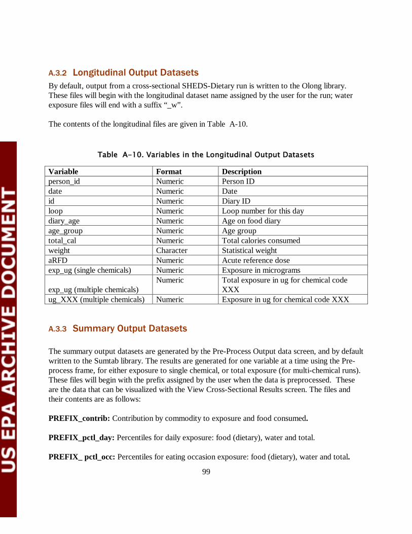
99

A.3.2 Longitudinal Output Datasets By default, output from a cross-sectional SHEDS-Dietary run is written to the Olong library. These files will begin with the longitudinal dataset name assigned by the user for the run; water exposure files will end with a suffix “_w”. The contents of the longitudinal files are given in Table A-10.

Table A-10. Variables in the Longitudinal Output Datasets

Variable Format Description person_id Numeric Person ID date Numeric Date id Numeric Diary ID loop Numeric Loop number for this day diary_age Numeric Age on food diary age_group Numeric Age group total_cal Numeric Total calories consumed weight Character Statistical weight aRFD Numeric Acute reference dose exp_ug (single chemicals) Numeric Exposure in micrograms

exp_ug (multiple chemicals) Numeric Total exposure in ug for chemical code

XXX ug_XXX (multiple chemicals) Numeric Exposure in ug for chemical code XXX

A.3.3 Summary Output Datasets The summary output datasets are generated by the Pre-Process Output data screen, and by default written to the Sumtab library. The results are generated for one variable at a time using the Pre-process frame, for either exposure to single chemical, or total exposure (for multi-chemical runs). These files will begin with the prefix assigned by the user when the data is preprocessed. These are the data that can be visualized with the View Cross-Sectional Results screen. The files and their contents are as follows: PREFIX_contrib: Contribution by commodity to exposure and food consumed. PREFIX_pctl_day: Percentiles for daily exposure: food (dietary), water and total. PREFIX_ pctl_occ: Percentiles for eating occasion exposure: food (dietary), water and total.

100

PREFIX_ summary_day: Summary percentiles for daily exposure by age group: food (dietary), water and total. PREFIX_ summary _occ: Summary percentiles for eating occasion exposure by age group: food (dietary), water and total. PREFIX_ tab_day: Daily exposure and percent %APAD percentiles by age group: food (dietary), water and total. PREFIX_ tab _occ: Eating occasion exposure and percent %APAD percentiles by age group: food (dietary), water and total.