Struct Multidisc OptimDOI 10.1007/s00158-013-1005-7

RESEARCH PAPER

The stiffness spreading method for layout optimizationof truss structures

Peng Wei · Haitao Ma · Michael Yu Wang

Received: 2 September 2012 / Revised: 8 September 2013 / Accepted: 19 September 2013© Springer-Verlag Berlin Heidelberg 2013

Abstract A novel optimization method, stiffness spread-ing method (SSM), is proposed for layout optimization oftruss structures. In this method, stiffness matrices of thebar elements in a truss structure are represented by a set ofequivalent stiffness matrices which are embedded in a weakbackground mesh. When the proposed method is used, itis unnecessary for the bar elements in a truss structure tobe connected to each other during the optimization process,and each of the bar elements can move independently in thedesign domain to form an optimized design. Another fea-ture of the method is that the sensitivity analysis can be doneanalytically, making gradient based optimization algorithmsapplicable in the solution. This method realizes the size,shape and topology design optimization of truss structuressimultaneously and allows for more flexibility in topologychange. Numerical examples illustrate the feasibility andeffectiveness of the proposed method.

The research work is supported by The National ScienceFoundation for Young Scientists of China (Grant Nos. 11002058and 11002056) and State Key Lab of Subtropical Building Science(SCUT) (Grant Nos. 2010ZA03 and 2012ZC22)

P. Wei (�) · H. MaState Key Laboratory of Subtropical Building Science,School of Civil Engineering and Transportation,South China University of Technology,Guangzhou, Chinae-mail: ctpwei@scut.edu.cn

M. Y. WangDepartment of Mechanical and Automation Engineering,The Chinese University of Hong Kong,Hong Kong, Chinae-mail: yuwang@cuhk.edu.hk

Keywords Layout optimization · Structural optimization ·Topology optimization · Truss structure

1 Introductions

The structural layout optimization means optimizing thesize, shape and topology of a structure simultaneously. It canbe considered as one of the most challenging set of problemsin structural optimization field. In this paper we focus onthe well-known optimal design of truss structures. The studyof the layout optimization of truss structures was pioneeredby Michell (1904), when he derived the exact solutions byanalytical method for some simple problems with stressconstraint. Although Michell’s pioneering work is of greatfundamental importance, it was neglected about 40 years.Until 1950s, Cox (1958), Hemp (1997), Prager and Rozvany(1977) and other researchers did systematic studies ofMichell trusses and the truss layout optimization theory hasbeen explored extensively in the following several decades.

The exact solutions are very important for subsequentstudies, but they are hard to be obtained for real worldengineering problems. The well-known ground structure (orstructural universe) approach proposed by Dorn et al. (1964)opened up a fruitful period of structural layout optimization.Ground structure denotes a union of all potential membersconnected between a set of nodal points. The optimizationis a procedure of eliminating inefficient members from theground structure with some criteria. The ground structureapproach converts the truss layout design problem into asize design problem. In recent years, a great number of stud-ies of truss layout optimization are based on the groundstructure approach.

In the ground structure approach, the number of designvariables grows dramatically as the number of nodal points

P. Wei et al.

is increased. Furthermore, the ground structure approachlimits the feasible design space of the problem at the begin-ning. As the number of the nodal points is finite, thefinal design obtained can only be a local optimum. Animproved approach incorporates the locations of the jointsas the design variables and the new model can optimizethe geometrical variables and sectional areas simultane-ously or iteratively (Pedersen 1972; Vanderplaats and Moses1972; Topping 1983) thus realizes the shape and topologyoptimization together.

Kirsch (1990) investigated the relationship between theshape and topology optimization problems. Later, Achtziger(2007) studied the difference between simultaneous anditerative strategies for the geometry and topology optimiza-tion of a truss structure. These approaches increase thechance to obtain better solutions and reduce the numberof variables to reduce the computational cost. More detailsabout the approaches can be found in the review paper ofRozvany et al. (1995), the monograph of Bendsøe andSigmund (2003) and a recent review paper of Rozvany(2011).

In this paper, the authors propose an innovative method,stiffness spreading method (SSM), to solve the truss layoutoptimization problem. In this method, a regular backgroundmesh is introduced in the design domain so that bar elementscan be put anywhere within this domain. The displacementsof the nodes of a bar element are related to those of thebackground mesh with radial basis function (RBF) interpo-lation (Buhmann 2004). Based on this RBF interpolation,stiffness matrices of bar elements are then transformed toequivalent stiffness matrices, which can be regarded as aspreading of the stiffness contribution of the bar elementsto the background mesh. Unlike the conventional shape andtopology optimization methods of truss structures, neitherthe ground structure nor the prior knowledge of the elementconnections and node locations is necessary. During theoptimization process, it is unnecessary for the bar elementsto be connected to each other and as a result, each ele-ment is allowed to move independently. This model offersthe bar elements very high freedom to assemble the opti-mized design with an optimization algorithm. This can beconsidered as a great improvement compared with the con-ventional layout optimization models for truss structuresbecause it eliminates the solution dependency on the ini-tial ground structure. This method and some preliminarynumerical examples were initially presented at the SixthChina-Japan-Korea Joint Symposium on Optimization ofStructural and Mechanical Systems (Wei et al. 2010).

Furthermore, as shown below, the proposed method inthis paper can be considered as optimizing a truss structureembedded in a very weak continuum mesh. This conceptcan also be implemented in reinforced concrete topologyoptimization. Amir and Sigmund (2013) have implemented

the ground structure method for solving this problem. Ahybrid routine combining truss and continuum topologyoptimization methodologies was also proposed by Gaynoret al. (2013) for reinforced concrete design. Zegard andPaulino (2013) solved this problem by embedding discretetruss members in a continuum based on a convolution oper-ator whose effect can be found very similar to that of theradial basis functions used in this paper. Thus it is verylikely that this method can be combined with these algo-rithms in solving these problems. A tentative approach hasbeen implemented in solving a similar layout optimizationproblem which considers simultaneously the sizes and posi-tions of discrete bar elements together with the topology ofa supporting continuum (Wei et al. 2012).

In this model, the sensitivities required for the opti-mization can be obtained analytically thus optimizationalgorithms based on mathematical programming methodscan be easily implemented. In this paper, the Method ofMoving Asymptotes (MMA) (Svanberg 2002) is applied asthe optimizer. The objective function is the strain energy.The design variables are defined as the nodal coordinatesand cross sectional areas of the bar elements. This paperis organized as follows. Firstly, a brief introduction of thetruss structure layout optimization is given. Then the stiff-ness spreading method and the interpolation approach withradial basis functions are presented. After that, some numer-ical examples and discussions are presented and finally theconclusions are given.

2 Optimization model

The optimization problem is defined as follows:

Find : x = {A, w}A = {A1, A2, · · · , An}w = {w1, w2, · · · , w2n}

Min : J = J (x, u(x))

s.t. K(x)u(x) = F (x)

V (x) ≤ V0 (1)

where x is the design variable vector which includes twoparts: A for the sectional areas of bar elements and w thenodal coordinates, n denotes the total number of the bar ele-ments, J is the objective function which is defined as thetotal strain energy of the structure, K(x) the stiffness matrix,u(x) the displacement vector, F(x) the load vector, V (x)the total volume of the structure, V0 the upper bound of thevolume of the designed structure.

The derivative of the objective function is

dJ

dx= ∂J

∂x+ ∂J

∂u· du

dx(2)

The SSM for truss layout optimization

When the total strain energy is taken as the objectivefunction, we have

J = 1

2uT · K · u (3)

By applying the adjoint method, (2) leads to

dJ

dx= −1

2uT · dK

dx· u + uT · dF

dx(4)

For the case when the load is independent of design vari-ables, namely dF/dx = 0, the sensitivities can be stated as

dJ

dx= −1

2uT · dK

dx· u (5)

The total volume of the truss structure is given as

V =n∑

i=1

Aili (6)

where n is the number of the bar elements, Ai the sectionalarea and li the length of the i-th element. Here Ai’s aredesign variables and li ’s are functions of nodal coordinateswhich are also to be optimized. The derivatives of the objec-tive function and the volume constraint with respect to thedesign variables can be easily obtained by using the aboveexpressions.

3 Stiffness spreading method

In this section, some implementation details of the stiff-ness spreading method (SSM) are presented. In SSM, thetruss structure is embedded in the design domain filled witha uniformly distributed weak material. The weak materialshould be modeled and included in the finite element anal-ysis together with the truss structure and the finite elementmesh representing the weak material part is called the back-ground mesh. The fundamental concept of the SSM is torepresent the nodal displacements of bar elements for a trussstructure in terms of displacements of the background meshduring the optimization process. Thus, even though two barsare not directly linked through a common node, they canstill be considered to be connected indirectly because thenodal displacements of both elements are related to nodaldisplacements of the background mesh. The connectionbetween these two bars depends on the type of the interpo-lation function and their relative positions. Therefore, theinfluence of one bar’s stiffness will not be limited to itstwo nodes but will also extend to the surrounding fields. Inother words, the stiffness of this element spread from its twonodes to those of the background mesh. More details of theSSM are given in the rest of this section.

3.1 Finite element model with interpolation

In a standard finite element procedure, the potential energyof a structure is

�p =∑

e

(aT

e ·∫

�e

1

2BT DBdV · ae

)

−∑

e

(aT

e ·∫

�e

NT f dV

)

−∑

e

(aT

e ·∫

�e

NT pdS

)(7)

where ae denotes the displacement vector of an element,B the element strain-displacement matrix, D the elasticitymatrix, N the shape function matrix of the element, f thebody force vector and p the traction force on the boundary� of the structure.

The element stiffness matrix is

Ke =∫

�e

BT DBdV (8)

and the equivalent nodal load vector is

F e =∫

�e

NT f dV +∫

�e

NT pdS (9)

If the displacement vector ae can be represented in terms ofanother displacement vectors ue with the following equation

ae = T · ue (10)

where T is the transformation matrix (7) can be written as:

�p =∑

e

(uT

e · T T · Ke · T · ue

)−

∑

e

(uT

e · T T · F e

)

(11)

The formation of T will be discussed in detail later.The element stiffness matrix after interpolation can be

written as:

K̃e = T T · Ke · T (12)

and the nodal load vector:

F̃ e = T T · F e (13)

The global stiffness matrix K of the truss structure is formedfrom the stiffness matrices of bar elements and the stiffnessmatrix for a 2D truss element can be written as:

Kei = EAi

li

⎡⎢⎢⎣

cos2θi cosθi sinθi

cosθi sinθi sin2θi

−cos2θi −cosθi sinθi

−cosθi sinθi −sin2θi

−cos2θi −cosθi sinθi

−cosθi sinθi −sin2θi

cos2θi cosθi sinθi

cosθi sinθi sin2θi

⎤⎥⎥⎦

(14)

where E is the Young’s modulus and θi is the slope angle ofthe i-th element in the coordinate system, see Fig. 1.

P. Wei et al.

Fig. 1 A 2D bar element

Thus the derivative of the i-th elemental stiffness matrixin the linear model with respect to the sectional area can beobtained with

∂Kei

∂Aj

=

⎧⎪⎨

⎪⎩

1

Aj

Kei i = j

0 i �= j

(15)

The derivative of Ke with respect to the coordinates of thenodes of a bar element can be obtained by the chain rule:

∂Kei

∂wj

= ∂Kei

∂l· ∂l

∂wj

+ ∂Kei

∂θ· ∂θ

∂wj

(16)

where wj (j = 1, 2, . . . , 2n) is the j-th component in thedesign variable vector for nodal coordinates, w. The deriva-tive is zero when wj is not for one of the end nodes ofelement.

As illustrated in Fig. 2, the displacement DOFs of abar element ae are interpolated with a set of displacementvector ue in the background mesh with (10). One straight-forward approach is to use the element shape function tomake the interpolation. However, our experience has shownthat the use of element shape functions is not suitable forthis framework because of their piecewise property andnon-smoothness. Therefore, we adopt the well-developedcompactly supported radial basis functions (CS-RBF) in thisstudy for its globally continuous and differentiable proper-ties which satisfy the requirement of our method very well.In the next section, a brief introduction about the radial basisfunctions method (RBF) is given for completeness.

Fig. 2 The transformation of DOFs

3.2 Radial basis functions modeling

Radial basis functions method is a well-developed method-ology to approximate or reconstruct an admissible designwith a set of basis functions which are globally continuousand differentiable. Some attractive features of radial basisfunctions such as the unique solvability of the interpolationproblem and their smoothness and convergence make themsuitable in the stiffness spreading model.

Radial basis functions are a set of radially-symmetricfunctions centered at particular points, or knots. Thesefunctions can be expressed as following:

gi(s) = g(||s − si ||), s ∈ Rd (17)

where s denotes coordinates of points in Euclidean spaceand ‖·‖ denotes the Euclidean norm on Rd , si is the positionof the i-th knot, and g : R+ → R with g(0) ≥ 0.

A large number of different radial basis functions areavailable and used in the engineering fields, which can beroughly divided into two classes, one is of the globally sup-ported radial basis functions (GS-RBF), including thin-platespline, polyharmonic splines, Sobolev splines, Gaussians,multiquadrics (MQ), inverse multiquadrics (IMQ) and soon, the other is of the compactly supported radial basisfunctions (CS-RBF) (Wu 1995; Wendland 1995). Althoughthe GS-RBF have many attractive features such as highernumerical accuracy hence the positive definite MQ and IMQhave been incorporated into the level set method to developthe ODEs type scheme (Luo et al. 2008), in this paper apopularly used CS-RBF (Wendland 1995), the one with C2

continuity, is chosen due to some practical advantages suchas the strictly positive definite property, sparsity of the sys-tem matrix, calculation efficiency, principle of locality andso on. The following C2 Wendland CS-RBF is chosen inpresent work

g(r) = (max(0, 1 − r))4 · (4r + 1) (18)

where radial distance r is given as:

r =√

(ξ − ξi)2 + (η − ηi)2

dsp

(19)

where dsp is a predefined constant known as the supportradius of the RBF and si = (ξi , ηi) is the 2D coordinate ofthe i-th knot point and s = (ξ, η) is the coordinate of thesample point. The derivative of this CS-RBF can be easilyobtained by the chain rule as follows:

∂g(ξ, η)

∂ξ= (max(0, 1 − r))3 · (−20r) · ∂r

∂ξ

∂g(ξ, η)

∂η= (max(0, 1 − r))3 · (−20r) · ∂r

∂η(20)

The SSM for truss layout optimization

a. A basis function of the C2 CS-RBF b. Partial derivative of the C2 CS-RBF in x direction

Fig. 3 The C2 CS-RBF and its partial derivative

The C2 CS-RBF and its derivative are shown in Fig. 3.A scalar function (s) can be represented with N basis

functions centered at N knots as:

(s) =N∑

i=1

gi(s)αi + p(s) (21)

where αi is the weight of the radial basis function posi-tioned at the i-th knot si , and p(s) a first-degree polynomialto account for the linear and constant portions of g(s) andto ensure polynomial precision (Buhmann 2004). For C2CS-RBF the polynomial is not needed, thus the (21) can bere-written as:

(s) =N∑

i=1

gi (s) αi (22)

or

(s) = gT (s)α (23)

where

g = [g1(s), g2(s), · · · , gN(s)]T (24)

α = [α1, α2, · · · , αN ]T ∈ RN×1 (25)

The coefficient vector α can be determined by solving thefollowing equation

H 0α = � (26)

where

H 0 =

⎡

⎢⎢⎢⎣

g1(s1) g2 (s1) · · · gN(s1)g1(s2) g2 (s2) · · · gN(s2)

.

.

....

. . ....

g1(sN ) g2 (sN ) · · · gN(sN )

⎤

⎥⎥⎥⎦ (27)

� =

⎡⎢⎢⎢⎣

φ1φ2...

φN

⎤⎥⎥⎥⎦

(28)

a. The node of a bar element is not coincident with a node of the background mesh.

b. The node of a bar element is coincident with a node of the background mesh.

Fig. 4 Spreading scheme of a node in one end of a bar element with CS-RBFs

P. Wei et al.

Fig. 5 A short cantilever beam design problem

and si denotes the location of the i-th knot. A thoroughlytheoretical implementation viewpoint on RBF can be foundin (Buhmann 2004).

3.3 Stiffness spreading method implementation with RBF

In RBF based interpolation, displacements everywhere canbe represented by a set of coefficients α and basis func-tions g(s). Here g(s) is a function of the locations of knots

Fig. 6 The iteration process of the short cantilever beam designproblem

and the sample points as show in (17). The interpolateddisplacement field can be expressed as

u(s) =N∑

i=1

gi (s) αi (29)

For a set of displacements (29) can be written in a matrixform,

u = H · α. (30)

In a framework with fixed knots and sample points, suchas both of them are on the nodes of the background grid(collocation), the H matrix is changed to H0 in (26) whichis also fixed. Thus

α = H−10 · u0 (31)

where u0 = {u1, u2, . . . , uN }T denotes the displace-ments of background mesh on the grid. According to (29),an interpolated displacement at location s can be written as

u(s) = {g1(s) · · · gN (s)} · H−10 ·

⎧⎪⎪⎪⎨

⎪⎪⎪⎩

u1

u2...

uN

⎫⎪⎪⎪⎬

⎪⎪⎪⎭(32)

According to (23), the displacements on the degrees of free-dom ae can be represented with the displacement vector u0

on the background grid as

⎧⎪⎪⎨

⎪⎪⎩

ae(s1)ae(s2)

.

.

.ae(sm)

⎫⎪⎪⎬

⎪⎪⎭=

⎡

⎢⎢⎣

g1(s1) g2(s1) · · · gN(s1)g1(s2) g2(s2) · · · gN(s2)

.

.

....

. . ....

g1(sm) g2(sm) · · · gN (sm)

⎤

⎥⎥⎦ · H−10 ·

⎧⎪⎪⎨

⎪⎪⎩

u1u2...

uN

⎫⎪⎪⎬

⎪⎪⎭

(33)

where si (i = 1, 2, . . . , m) denotes the coordinates of loca-tions where the displacements are interpolated as shown inFig. 2. Then it can be easily find that in (10)

T =

⎡

⎢⎢⎢⎣

g1(s1) g2(s1) · · · gN(s1)

g1(s2) g2(s2) · · · gN(s2)...

.... . .

...

g1(sm) g2(sm) · · · gN(sm)

⎤

⎥⎥⎥⎦ · H−10 (34)

Substituting (34) into (12), we can calculate the transformedstiffness matrix with RBF interpolation. Figure 4 illustratesthe spreading effect of a bar element in the backgroundmesh with CS-RBF. If the node of a bar element is not coin-cident with a node of the background mesh as shown inFig. 4a, the stiffness contribution of the bar element is addedinto the background elements which are connected to thenodes with red color. The big red circle indicates the sup-port area of the CS-RBF which is centered on the end ofthe bar element. The nodes of red color in the backgroundmesh are surrounded by the circle. The degree of influence

The SSM for truss layout optimization

Table 1 The initial andoptimal design of the shortcantilever beam design problem

Coordinates of node1 Coordinates of node2 Sectional areas

Initial design Bar 1 (1.5000, −3.0000) (3.5000, −3.0000) 1.0000

Bar 2 (1.5000, 3.0000) (3.5000, 3.0000) 1.0000

Optimal design Bar 1 (0.0002, −4.9998) (4.9997, −0.0068) 0.2831

Bar 2 (0.0002, 4.9999) (4.9997, 0.0068) 0.2831

of the bar’s stiffness to each node depends on the interpo-lation function, namely the CS-RBF in this paper, and thedistance between the nodes in the background mesh andthe node of the bar element. In the case of the node of abar element being coincident with one node of the back-ground mesh, the spreading approach takes no effect andthe bar element can be considered just being connectedto that node in the background mesh. This property canalso be easily developed from (33) in which if si = si ,ae(si) is precisely equal to ui . Thus the corresponding vec-tor in T matrix will be a unit vector with only one unitelement at i and according to (12) the stiffness matrix of thebar element is originally added into the background meshin FEA model without spreading. This is a very impor-tant property of the proposed method which indicates asmooth transition between connecting and disconnectingof the nodes in background mesh and the bar element.This property provides an approximate FEA approach offree layout of discrete components in a continuous struc-ture without considering the way of connections betweenthem and this is very important for layout optimization. Therelated sensitivities can be easily obtained as shown in whatfollows.

Considering a design variable x which may be the nodalcoordinate or the sectional area of a bar element, the sensi-tivity leads to

dK

dx=

∑

i∈Js

d

dx

(T T · Kei · T

)(35)

where Js is the set of indices of the bar elements which arerelated to the design variable x. Since T = T(x), it can befound that

dKdx

=∑

i

(∂TT

∂x· Kei

· T + TT · ∂Kei

∂xT + TT Kei

· ∂T∂x

)(36)

where

∂T

∂x=

⎡

⎢⎢⎢⎢⎢⎢⎢⎣

∂g1(x)

∂x

∂g2(x)

∂x· · · ∂gn(x)

∂x∂g1(x)

∂x

∂g2(x)

∂x· · · ∂gn(x)

∂x...

.... . .

...∂g1(x)

∂x

∂g2(x)

∂x· · · ∂gn(x)

∂x

⎤

⎥⎥⎥⎥⎥⎥⎥⎦

· H−10 (37)

It can be easily found that ∂T/∂x = 0 if x denotes a sectionalarea.

Fig. 7 The iteration history ofthe objective function andvolume constraint

P. Wei et al.

Fig. 8 The optimal results withdifferent initial designs

Substituting (36) and (37) into (5), the derivatives ofthe objective with respect to the design variables can beeasily obtained. According to (6), the derivatives of the vol-ume constraint with respect to the design variables can alsobe obtained. Based on the sensitivity analysis results pre-sented above, gradient based optimization methods can beimplemented in the SSM based model to solve the layoutoptimization problem of truss structures. In this paper, themethod of moving asymptotes (MMA) is used for solvingthe following numerical examples (Svanberg 2002).

4 Numerical examples

In this section, several numerical examples are presented toshow the properties of the SSM. The first model considered

Fig. 9 The optimal results with mesh size 5 × 20

is a short cantilever beam design problem as shown inFig. 5. The left end of the beam is fixed and a vertical loadF = 105 is applied at the middle of the right end. In thepresent work, the stiffness maximization problem is consid-ered by minimizing the total strain energy of the structure.

Fig. 10 The strain energy test of the 2-bar problem with respect to thenodal locations and the support radii of RBF

The SSM for truss layout optimization

Fig. 11 The possible locationsof local minimum

Firstly we consider the case of putting only 2 bars intothe design domain. The optimization process is illustratedin Fig. 6 and the iteration history of the objective func-tion and the volume constraint are shown in Fig. 7. Table 1shows the initial and optimal designs of this problem. Thedesign domain is divided into a 5 × 10 background mesh.The knots of the RBFs are coincident with the nodes in thebackground mesh grid. A support radius of 4-element sizeis used. In this case, the maximum number of iterations isfixed at 50.

According to the iteration history shown in Fig. 7, theiteration process converged after about 40 steps. The totalvolume of the bars is set the same as the initial design and itis satisfied well after convergence as illustrated.

Solutions with different initial designs of this problemhave also been obtained and are shown in Fig. 8. Two barremoval schemes are implemented to remove the bars whichare considered useless. One scheme is to remove a bar if itscross sectional area is less than a lower bound Aε, and theanother one is to remove a bar if its length is below a lower

Fig. 12 The influence of thesupport radius on the structure’sstrain energy

P. Wei et al.

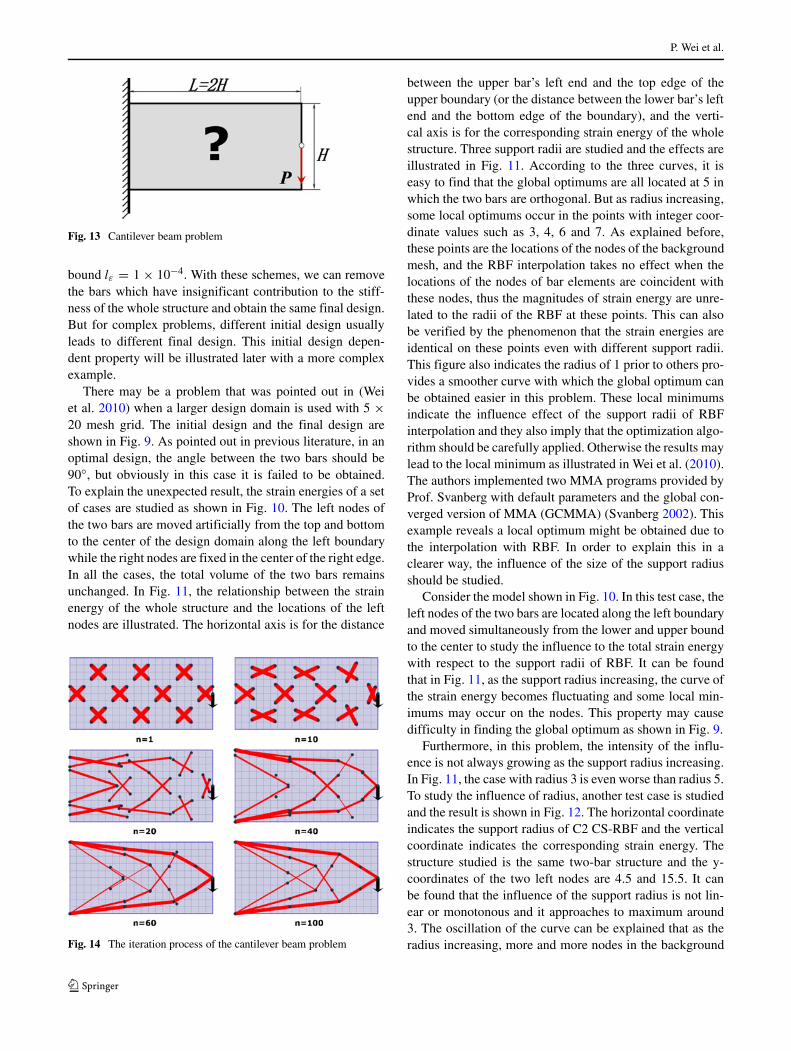
Fig. 13 Cantilever beam problem

bound lε = 1 × 10−4. With these schemes, we can removethe bars which have insignificant contribution to the stiff-ness of the whole structure and obtain the same final design.But for complex problems, different initial design usuallyleads to different final design. This initial design depen-dent property will be illustrated later with a more complexexample.

There may be a problem that was pointed out in (Weiet al. 2010) when a larger design domain is used with 5 ×20 mesh grid. The initial design and the final design areshown in Fig. 9. As pointed out in previous literature, in anoptimal design, the angle between the two bars should be90◦, but obviously in this case it is failed to be obtained.To explain the unexpected result, the strain energies of a setof cases are studied as shown in Fig. 10. The left nodes ofthe two bars are moved artificially from the top and bottomto the center of the design domain along the left boundarywhile the right nodes are fixed in the center of the right edge.In all the cases, the total volume of the two bars remainsunchanged. In Fig. 11, the relationship between the strainenergy of the whole structure and the locations of the leftnodes are illustrated. The horizontal axis is for the distance

Fig. 14 The iteration process of the cantilever beam problem

between the upper bar’s left end and the top edge of theupper boundary (or the distance between the lower bar’s leftend and the bottom edge of the boundary), and the verti-cal axis is for the corresponding strain energy of the wholestructure. Three support radii are studied and the effects areillustrated in Fig. 11. According to the three curves, it iseasy to find that the global optimums are all located at 5 inwhich the two bars are orthogonal. But as radius increasing,some local optimums occur in the points with integer coor-dinate values such as 3, 4, 6 and 7. As explained before,these points are the locations of the nodes of the backgroundmesh, and the RBF interpolation takes no effect when thelocations of the nodes of bar elements are coincident withthese nodes, thus the magnitudes of strain energy are unre-lated to the radii of the RBF at these points. This can alsobe verified by the phenomenon that the strain energies areidentical on these points even with different support radii.This figure also indicates the radius of 1 prior to others pro-vides a smoother curve with which the global optimum canbe obtained easier in this problem. These local minimumsindicate the influence effect of the support radii of RBFinterpolation and they also imply that the optimization algo-rithm should be carefully applied. Otherwise the results maylead to the local minimum as illustrated in Wei et al. (2010).The authors implemented two MMA programs provided byProf. Svanberg with default parameters and the global con-verged version of MMA (GCMMA) (Svanberg 2002). Thisexample reveals a local optimum might be obtained due tothe interpolation with RBF. In order to explain this in aclearer way, the influence of the size of the support radiusshould be studied.

Consider the model shown in Fig. 10. In this test case, theleft nodes of the two bars are located along the left boundaryand moved simultaneously from the lower and upper boundto the center to study the influence to the total strain energywith respect to the support radii of RBF. It can be foundthat in Fig. 11, as the support radius increasing, the curve ofthe strain energy becomes fluctuating and some local min-imums may occur on the nodes. This property may causedifficulty in finding the global optimum as shown in Fig. 9.

Furthermore, in this problem, the intensity of the influ-ence is not always growing as the support radius increasing.In Fig. 11, the case with radius 3 is even worse than radius 5.To study the influence of radius, another test case is studiedand the result is shown in Fig. 12. The horizontal coordinateindicates the support radius of C2 CS-RBF and the verticalcoordinate indicates the corresponding strain energy. Thestructure studied is the same two-bar structure and the y-coordinates of the two left nodes are 4.5 and 15.5. It canbe found that the influence of the support radius is not lin-ear or monotonous and it approaches to maximum around3. The oscillation of the curve can be explained that as theradius increasing, more and more nodes in the background

The SSM for truss layout optimization

Fig. 15 Iteration histories ofobjective function and totalvolume for the long cantileverbeam problem

mesh are surrounded in the support area of the RBF. Oncea new node joins in the support area, the stiffness spreadingeffect will change correspondingly. Because of this prop-erty, the support radius should be chosen carefully to reducethe effect of local minimum.

A long cantilever beam problem shown in Fig. 13 is stud-ied. The left side of the beam is fixed and a concentratedforce is applied at the middle of the right side. Here H =

10 and L = 20. A 20 × 10 background mesh is used inthis problem and the knots of RBF for interpolation areplaced on the nodes of the mesh. The Young’s modulus ofthe bars is 1,000 times the one of the background mate-rial. The C2 CS-RBF with the support radius 2.2 elementssize is used. The initial design and five designs obtainedduring the iteration process of the optimization are illus-trated in Fig. 14. The solution converges in about 100 steps.

Table 2 The initial and final designs of the cantilever beam problem with different support radii

Initial design

Number of bars 20 40 42

Support radius = .5× element size

Strain energy 2.309 × 10−3 2.730 × 10−3 3.056 × 10−3

Support radius = 3.5 × element size

Strain energy 3.094 × 10−3 2.898 × 10−3 3.801 × 10−3

Support radius = 4.5 × element size

Strain energy 2.722 × 10−3 2.978 × 10−3 3.807 × 10−3

P. Wei et al.

Table 3 The cantilever beam problem compared with ground structure method

Initial design

Final design (200 iterations)

Optimization model SSM Ground structure with Groud structure with

fixed nodal positions movable nodal positions

Number of bars 20 36 36

Computation time (s) 857 306 336

Strain energy 2.31 × 10−3 2.70 × 10−3 2.17 × 10−3

During the iteration, each bar element moves independentlyfrom the initial location to the final position. The changesof the bars’ sectional areas can also be easily seen from thefigures. The stiffness spreading method realizes the size,shape and topology optimization simultaneously in thisproblem. It should be noted that, in the converged design,the two bar elements located in the same line and with onenode of each overlapped should be considered as one ele-ment because a bar element can only sustain axial force.Thus this 20-bar truss structure is actually a 10-bar trussstructure in this model. The iteration history of the objectivefunction and the total volume are shown in Fig. 15.

A reasonably result is shown in Fig. 14. Unfortunately,the optimized results may sometimes be sensitive to solutionparameters, such as the support radius of RBF, the initiallayout of bars, the parameters in MMA program and so on.This means that the users may have to tune the parametersto get a better final result. The existence of this problem isnot hard to understand: in each iteration step, the locationof each node may greatly influence the follow-up layout ofthe truss. Some optimized results are presented in Table 2 toillustrate the influence of the support radius and the initialdesign with the same example.

In Table 2, optimal results for different initial designsand support radii in RBF interpolation are presented. Thesupport radii used in RBF are chosen as 2.5, 3.5 and 4.5times of the background mesh size and three initial designsare considered. The first initial design has 20 bars, the sec-ond one has 40 bars and the third one has 42 bars. For eachsolution, 200 iterations are allowed. Note that, because thebar-deleting scheme has not been implemented, some “use-less” bars are still present in the final designs. According tothis table, the optimal topology with the first initial designchanges greatest as the support radius increases while thesecond and the third ones do not change so much. Thisindicates the more the number of bars in the initial design,

the less the influence of the support radius. This table alsoillustrates the influence of the initial design on the designobtained. This arouses an important issue about how toinvolve new bars into the design domain. Theoretically, theFEA of the background structure provides some mechani-cal information, such like the strain energy density, in thewhole design domain. And this information could be usedin applying some ways to introducing new bars in appro-priate positions during optimization process. For this issue,further studies are still needed to improve the ability of theproposed method to obtain a true optimum.

Table 3 illustrates a comparison of the proposed methodwith the ground structure approach. Here two schemes areimplemented in ground structure: one considers only theoptimization of the sectional areas, the other considers theoptimization of the sectional areas and the nodal positions.The boundary and load conditions, the material propertiesand the volume constraints of these three problems are thesame. All of these problems are solved using MMA forfair comparison. The results reflect the relatively lower effi-ciency of the SSM because the FEA and sensitivity analysisin this model are time consuming. The objective functionresults illustrate in this example the result of SSM is supe-rior to the ground structure method in which the nodalpositions are fixed, but not as good as the one in which

Fig. 16 Simple supported beam with a downward force

The SSM for truss layout optimization

the nodes are movable. The spreading scheme endows thismodel a gift with much flexible topology modification butit also involves approximation to prevent it approach thereal optimum of the original truss optimization problem.The computation times shows the efficiency of the proposedmethod is much lower than the traditional truss optimizationmethods. For this problem, methods of linear programming(LP) and optimality criteria (OC) are even faster than MMA.The lower efficiency is mainly due to the computation of thebackground mesh and the transformation matrix T and itsderivatives. The efficiency might not be acceptable in solv-ing 3D problems. Thus it is an important issue to improvethe computation efficiency and the interpolation scheme forsolving complex problems.

Based on the proposed method, another problem shownin Fig. 16 is studied. A downward force is applied at themiddle of the bottom edges of a simple supported beam. Thesame meshes and knots distribution scheme are adopted asin the previous example. A support radius of 6 elements sizeis used. The sectional area of every bar element in the initialdesign is 1.

Figure 17 shows the layout of the bars during the opti-mization process and Fig. 18 shows the iteration historyof the objective functions and the total volumes. As shownin the figure the volume constraint is applied to keep thetotal volume of the final design to be the same as the ini-tial design. Here a bar deleting scheme is applied, thereforethe initial design has 20 bars while there are only 14 barsleft after convergence because 6 bars have been deleted in

the optimization process. For the final design, it should benoticed that the four bars at the top lap over each other sothat they look not as thick as they should be. This can beobserved more clearly in the figure of step 60. This solutionconverges in less than 200 steps as shown in Fig. 18.

Figure 19 shows the layout optimization process of thesame problem with a different initial design which includes40 bars. The initial sectional area of each bar is

√2/2 to

keep the total volume same as in the previous example.Figure 20 illustrates the iteration history of the objectivefunction and the total volume. The deleting scheme is alsoapplied and finally 20 bars are deleted after optimization.The optimized objective function is very close to the onein the previous example, but it can be found that there isa little difference in the topologies between these two finaldesigns. Compared these final designs with those in theliterature, both of the final designs are reasonable but thedifference implies that the initial design dependence is hardto be completely avoided in this method.

5 Future works

While advantages of the proposed method in solving lay-out optimization problems of truss structures are obvious,there are still issues which should be further investigatedin the future. One of them is the setting of the supportradii of the radial basis functions. As discussed before, thesize of the support radius decides how the stiffness of a

Fig. 17 The iteration process ofthe optimization design

P. Wei et al.

Fig. 18 The iteration history ofthe objective function andvolume constraint

bar element is spread and then affects the final results. Theauthors have done some research work on this but so farhave not found a strategy to make a perfect choice of thesize. However, the authors have found that a relative large

value for support radius may help to get a more stable solu-tion. A value of 2 to 6 times the background element sizeis suggested. Besides, the size of the support radius influ-ences the final topology greatly for complex problems. This

Fig. 19 The iteration process ofthe optimization design

The SSM for truss layout optimization

Fig. 20 The iteration history ofthe objective function andvolume constraint

issue is very important for successful applications of themethod.

Another issue is associated with the extending of the pro-posed method to 3D optimization problems. Obviously a 3Dbackground mesh is needed for 3D problems, and thus thecomputation time may increase dramatically. Therefore thisframework must be improved to be truly applicable for large3D design problems. A related study was reported in Caoet al. (2012).

6 Conclusions

In this paper, the authors propose a novel method, the stiff-ness spreading method, for layout optimization of trussstructures. Unlike the conventional shape and topologyoptimization design methods, the new method needs nei-ther the ground structure nor the prior knowledge of thenodes connections and locations. Based on the interpo-lation scheme with radial basis functions, the nodal dis-placements of bar elements are correlated with those ofthe background structure. As illustrated in the numericalexamples, the bar elements are not necessary to be con-nected to each other during the optimization process. Allthe sensitivity can be calculated analytically and gradi-ent based optimization algorithms can be used with thismodel, e.g. MMA. This model provides an entirely new con-cept to realize the size, shape and topology optimizationtogether for truss structures. The feasibility and effective-

ness of the proposed stiffness spreading method are illus-trated with the numerical examples. Finally, there are still afew issues which require further studies, such as the solu-tion efficiency, local minimum, initial design dependencyproblems.

Acknowledgments The authors are grateful to Prof. Krister Svan-berg for providing his MMA codes.

References

Achtziger W (2007) On simultaneous optimization of truss geometryand topology. Struct Multidiscip Optim 33:285–304

Amir O, Sigmund O (2013) Reinforcement layout design for con-crete structures based on continuum damage and truss topologyoptimization. Struct Multidiscip Optim 47:157–174

Bendsøe MP, Sigmund O (2003) Topology optimization: theory, meth-ods, and applications. Springer, Berlin Heidelberg

Buhmann MD (2004) Radial basis functions: theory and Implementa-tions. Cambridge University Press, New York

Cao M, Ma H, Wei P (2012) Modified stiffness spreading method forlayout optimization of truss structures. The 7th China-Japan-Koreajoint symposium on optimization of structural and mechanicalsystems, Huangshan

Cox HL (1958) The theory of design. Report of Aeronautical ResearchCouncil, No 2037

Dorn W, Gomory R, Greenberg H (1964) Automatic design of optimalstructures. J de Mechanique 3:25–52

Gaynor AT, Guest JK, Moen CD (2013) Reinforced concrete forcevisualization and design using bilinear truss-continuum topologyoptimization. J Struct Eng 139(4):607–618

Hemp WS (1997) Optimum structures. Clarendon, Oxford

P. Wei et al.

Kirsch U (1990) On the relationship between optimum structuraltopologies and geometries. Struct Optim 2:39–45

Luo Z, Wang MY, Wang SY, Wei P (2008) A level set-based parametrization method for structural shape and topologyoptimization. Int J Numer Methods Eng 76(1):1–26

Michell AGM (1904) The limits of economy of material in frame-structures. Phil Mag 8(6):589–597

Prager W, Rozvany GIN (1977) Optimal layout of grillages. J StructMech 5(1):1–18

Pedersen P (1972) On the optimal layout of multi-purpose trusses.Comput Struct 2:659–712

Rozvany GIN, Bendsøe MP, Kirsch U (1995) Layout optimization ofstructures. Appl Mech Rev 48(2):41–119

Rozvany GIN (2011) A review of new fundamental principles inexact topology optimization. In: Proceedings of 19th InternationalConference on Computer Methods in Mechanics, Warsaw

Svanberg K (2002) A class of globally convergent optimizationmethods based on conservative convex separable approximations.SIAM J Optim 12(2):555–573

Topping BHV (1983) Shape optimization of skeletal structures: areview. J Struct Eng ASCE 109(8):1933–1951

Vanderplaats GN, Moses F (1972) Automated design of trusses foroptimum geometry. J Struct Div 98(3):671–690

Wei P, Ma H, Chen T, Wang MY (2010) Stiffness spreading methodfor layout optimization of truss structures. In: Proceedings ofthe 6th China-Japan-Korea joint symposium on optimization ofstructural and mechanical systems, Kyoto

Wei P, Shi J, Ma H (2012) Integrated layout optimization design ofmulti-component systems based on the stiffness spreading method.In: Proceedings of the 7th China-Japan-Korea joint symposium onoptimization of structural and mechanical systems, Huangshan

Wendland H (1995) Piecewise polynomial, positive definite and com-pactly supported radial functions of minimal degree. Adv ComputMath 4:389–396

Wu Z (1995) Multivariate compactly supported positive definite radialfunctions. Adv Comput Math 4:283–292

Zegard T, Paulino GH (2013) Truss layout optimization within acontinuum. Struct Multidiscip Optim 48(1):1–16