The Steinberg Complex of an Arbitrary Finite Group inArbitrary Positive Characteristic

A DISSERTATION

SUBMITTED TO THE FACULTY OF THE GRADUATE SCHOOL

OF THE UNIVERSITY OF MINNESOTA

BY

Daniel E Swenson

IN PARTIAL FULFILLMENT OF THE REQUIREMENTS

FOR THE DEGREE OF

Doctor Of Philosophy

Peter J Webb

August, 2009

c© Daniel E Swenson 2009

ALL RIGHTS RESERVED

Acknowledgments

I would like to offer my heartfelt thanks to the many people who have helped me to

complete this project.

First, thank you very much to the countless kind people who have discussed this

project with me and shared their own insights. In particular, thank you to everyone

whom I was privileged to get to know at the Mathematical Sciences Research Institute

in Spring 2008.

Second, I would like to thank my older brother, Prof. James Swenson, for helping

me to discover the joys and wonders of mathematics and life. From the time I learned

to count through the present day, James has been a constant source of guidance and

strength for me.

Finally, I must thank my adviser, Prof. Peter Webb, for his patience, wisdom,

advice, and mathematical expertise. I truly appreciate the kindness and the hours of

discussion he has shared with me.

i

Dedication

To my parents.

ii

Contents

Acknowledgments i

Dedication ii

List of Figures v

1 Introduction 1

2 Subgroup complexes 4

3 The Steinberg complex: existence 10

4 Alternative complexes 26

5 Explicit calculations of a Steinberg complex, part I 28

6 Explicit calculations of a Steinberg complex, part II 35

7 Explicit calculations of a Steinberg complex, part III 39

8 Explicit calculations of a Steinberg complex, part IV 43

9 A subgroup of this wreath product 54

10 Another Steinberg complex with non-projective homology 56

11 A minimal group with non-projective Steinberg complex homology 59

iii

12 A further look at coefficient systems 75

References 83

Appendix A. GAP routines used in calculations 89

iv

List of Figures

2.1 Subgroup complexes for G = D12 at p = 2 . . . . . . . . . . . . . . . . . 7

3.1 The natural transformation condition . . . . . . . . . . . . . . . . . . . 16

7.1 A local view of a subspace U of |B3(W )| . . . . . . . . . . . . . . . . . . 41

7.2 A local view of the subspace U , deformed . . . . . . . . . . . . . . . . . 41

12.1 A commutative diagram involving exact sequences . . . . . . . . . . . . 78

12.2 The Eilenberg-Zilber theorem for Coefficient Systems . . . . . . . . . . . 80

v

Chapter 1

Introduction

The Steinberg complex is a generalization, to the case of an arbitrary finite group, of the

Steinberg module of a finite group of Lie type. Given a finite group G, a prime number

p, and a field R of characteristic p, one may build the Steinberg complex StRp (G), which

is a complex of projective RG-modules. If G happens to be a finite group of Lie type

over characteristic p, then the Steinberg complex will be the zero module everywhere,

except in a certain dimension, where it will be the Steinberg module. This is why the

Steinberg complex deserves its name.

In Chapter 2 of this paper we give some background information and definitions

necessary to define the Steinberg complex. Much of this is topological in nature, because

the definition of the Steinberg complex involves a simplicial complex ∆ with a G-action.

Stripping away some extraneous information from ∆ then yields the Steinberg complex.

This process is completely analogous to the case of a finite group of Lie type, where

one defines a topological space called the building, of which the top homology gives the

classical Steinberg module.

In Chapter 3 we prove a generalization of an important theorem of Webb. Webb’s

theorem is the process by which we strip away the extra information from ∆ to define

the Steinberg complex. It says that if a bounded CW-complex ∆ has a G-action with

certain properties, then the chain complex of RG-modules C∗(∆;R) decomposes as

direct sum of two complexes D∗ ⊕ P∗, where D∗ is chain-homotopy equivalent to the

zero complex and P∗ is a complex of projective RG-modules.

We prove that the theorem holds even if ∆ is infinite-dimensional, which allows

1

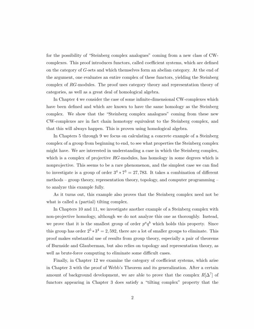
for the possibility of “Steinberg complex analogues” coming from a new class of CW-

complexes. This proof introduces functors, called coefficient systems, which are defined

on the category of G-sets and which themselves form an abelian category. At the end of

the argument, one evaluates an entire complex of these functors, yielding the Steinberg

complex of RG-modules. The proof uses category theory and representation theory of

categories, as well as a great deal of homological algebra.

In Chapter 4 we consider the case of some infinite-dimensional CW-complexes which

have been defined and which are known to have the same homology as the Steinberg

complex. We show that the “Steinberg complex analogues” coming from these new

CW-complexes are in fact chain homotopy equivalent to the Steinberg complex, and

that this will always happen. This is proven using homological algebra.

In Chapters 5 through 9 we focus on calculating a concrete example of a Steinberg

complex of a group from beginning to end, to see what properties the Steinberg complex

might have. We are interested in understanding a case in which the Steinberg complex,

which is a complex of projective RG-modules, has homology in some degrees which is

nonprojective. This seems to be a rare phenomenon, and the simplest case we can find

to investigate is a group of order 34 ∗ 73 = 27, 783. It takes a combination of different

methods – group theory, representation theory, topology, and computer programming –

to analyze this example fully.

As it turns out, this example also proves that the Steinberg complex need not be

what is called a (partial) tilting complex.

In Chapters 10 and 11, we investigate another example of a Steinberg complex with

non-projective homology, although we do not analyze this one as thoroughly. Instead,

we prove that it is the smallest group of order paqb which holds this property. Since

this group has order 25 ∗34 = 2, 592, there are a lot of smaller groups to eliminate. This

proof makes substantial use of results from group theory, especially a pair of theorems

of Burnside and Glauberman, but also relies on topology and representation theory, as

well as brute-force computing to eliminate some difficult cases.

Finally, in Chapter 12 we examine the category of coefficient systems, which arise

in Chapter 3 with the proof of Webb’s Theorem and its generalization. After a certain

amount of background development, we are able to prove that the complex R[∆?] of

functors appearing in Chapter 3 does satisfy a “tilting complex” property that the

2

Steinberg complex (which is obtained by uniformly evaluating the complex R[∆?]) lacks.

3

Chapter 2

Subgroup complexes

Definition 2.1 Let G be a group. A G-poset is a partially-ordered set Y together with

a G-action, such that for all a, b ∈ Y and for all g ∈ G, if a ≤ b then g · a ≤ g · b.A map of G-sets is a function f : X → Y where X and Y are G-sets, such that

f(g · x) = g · f(x) for all g ∈ G and x ∈ X. A map of posets is a function f : X → Y

where X and Y are posets, such that for all x, y ∈ X, if x ≤ y then f(x) ≤ f(y). A

map of G-posets is a function X → Y where X and Y are G-posets, such that f is a

map of G-sets and a map of posets.

Example: Let G be a finite group, and p a prime. We will write Sp = Sp(G) to denote

the poset of nontrivial p-subgroups of G, with the order relation given by inclusion of

subgroups. Then Sp is a G-poset under the (left) G-action given by conjugation.

Definition 2.2 Let G be a group. A G-simplicial complex is a simplicial complex ∆

together with a G-action, such that for each simplex σ of ∆ and each g ∈ G, the image

g · σ is a simplex of G, and if g fixes σ setwise then g fixes σ pointwise.

A map of simplicial complexes is a function f : X → Y where X and Y are simplicial

complexes, such that f sends each simplex of X to a simplex of Y by a linear map which

maps vertices to vertices. A map of G-simplicial complexes is a function f : X → Y

where X and Y are G-simplicial complexes, such that f is a map of simplicial complexes

and f is a map of G-sets.

Now let G be a finite group, and Y a G-poset. We define the order complex of Y to

4

be the simplicial complex whose n-simplices are exactly the totally-ordered subsets

P0 < P1 < . . . < Pn

in Y , for each n ≥ 0. Then Y is a G-simplicial complex.

Further, a map f : X → Y of G-posets induces a map |f | : |X| → |Y | of G-simplicial

complexes.

Definition 2.3 Let X and Y be G-simplicial complexes, and let α, β : X → Y be maps

of G-simplicial complexes. We say that α and beta are G-homotopic if there is a map

F : X×I → Y of G-simplicial complexes, where I is the closed interval [0, 1] with trivial

G-action, such that F (x, 0) = α(x) and F (x, 1) = β(x) for all x ∈ X. In this case F is

called a G-homotopy.

Example: If G is a non-identity p-group, then |Sp| is contractible, by a homotopy

which drags every vertex P0 < G along its edge to the vertex G, and leaves the vertex G

fixed throughout. It turns out that we may choose this homotopy to be a G-homotopy.

Let X = |Sp|, and let α : X → ∗ be the unique map, and let β : ∗ → X be the map

which sends the point ∗ to the vertex G. Of course α β is the identity on ∗, so we

just need to find a homotopy between the constant map β α : x 7→ G and the identity

map x 7→ x. We let F (x, t) = (1 − t) ∗ x + t ∗ G, using barycentric coordinates. Then

checking the definitions shows that F is a G-homotopy.

This example may be generalized. Recall that Op(G) denotes the maximal normal

p-subgroup of G, which is given by the intersection of all Sylow p-subgroups of G. Then:

Theorem 2.4 ([33] 2.4). If Op(G) 6= 1, then |Sp| is G-contractible.

Proof: A G-contraction takes a vertex P and moves it first up to the vertex POp(G),

then down to Op(G). Note that POp(G) is a nonidentity p-subgroup because Op(G) is

normal (and P and Op(G) are nonidentity p-subgroups).

The converse is also true: If Sp is G-contractible, then Op(G) 6= 1. Quillen conjec-

tured a stronger statement: If Sp is contractible (not necessarily G-contractible), then

Op(G) 6= 1. Quillen’s Conjecture has been proven in many cases but remains unproven

in general. Note that for the proof above we needed Op(G) to be non-trivial so that it

would be a vertex in |Sp|.

5

In proving this theorem, Quillen introduced another complex, Ap(G), which we wish

to define now along with several other complexes.

Definition 2.5 (i) Let Ap(G) denote the poset of nontrivial elementary abelian p-

subgroups of G. This is the subposet of Sp(G) whose objects are the subgroups of G

isomorphic to a direct product of a positive number of cyclic groups of order p.

(ii) Let Zp(G) denote the subposet of Ap(G) consisting of objects P satisfying P =

〈x ∈ Op(Z(CG(P ))) : xp = 1〉.(iii) Let Bp(G) denote the subposet of Sp(G) consisting of objects P satisfying P =

Op(NG(P )).

(iv) Let Rp(G) denote the simplicial complex whose vertices are the nonidentity

p-subgroups of G and whose n-simplices are exactly the chains of normal inclusions,

meaning that the n-simplices are all chains of the form K0 < K1 < . . . < Kn such that

Ki / Kn for all i. (Note that the normal subgroup relation is not transitive. However,

A / C and A < B < C imply A / B, so that each nonempty subset of the vertices of a

simplex is itself a simplex.)

(v) [1] Let Cp(G) denote the complex whose vertices are the subgroups of G of order

p and whose n-simplices are the sets of n+1 such subgroups which centralize each other.

Theorem 2.6 ([1], [9], [33], [6], [49]). |Sp(G)|, |Ap(G)|, |Zp(G)|, |Bp(G)|, Rp(G),

and Cp(G) are all G-homotopy-equivalent.

This theorem allows us to consider whichever of these G-equivalent spaces is most

convenient for the purpose at hand: often using the smaller posets Ap, Bp, and Rp can

make calculation substantially easier. Further, theorems like the one of Quillen’s above

may be proven just once rather than several times.

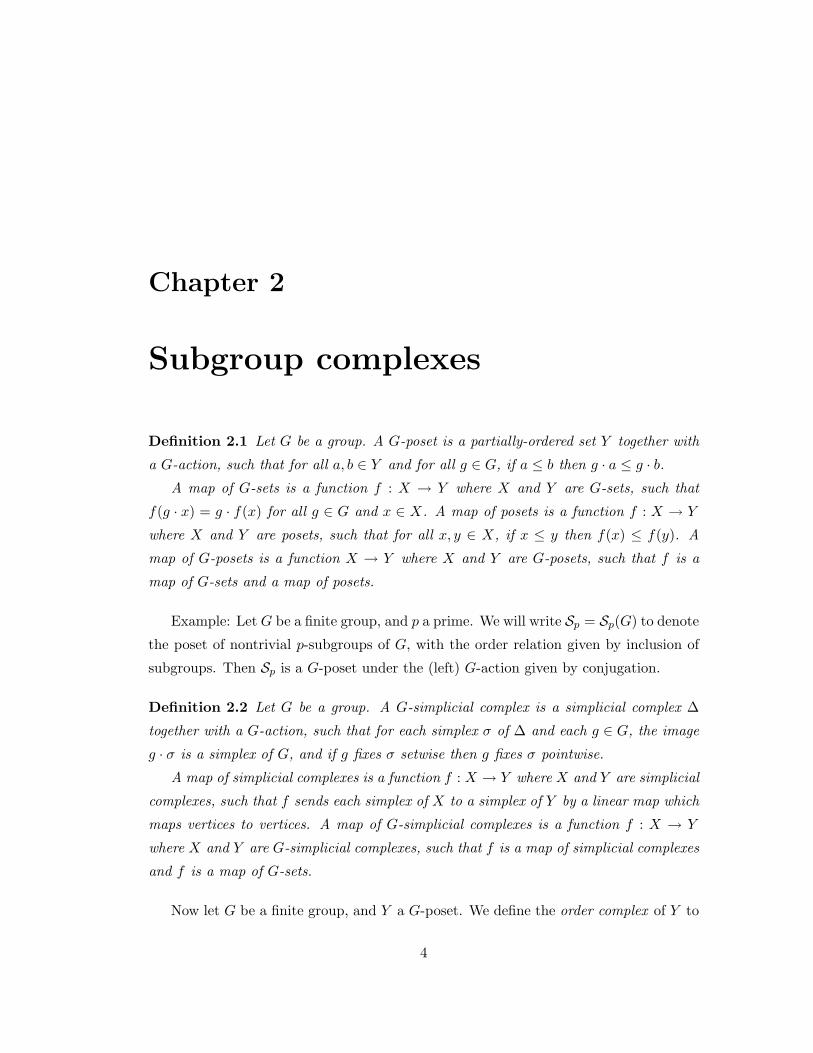
As an example, take G = D12 to be the dihedral group with 12 elements, and p = 2.

D12 has 3 Sylow 2-subgroups isomorphic to V4 (one of these is generated by a horizontal

and a vertical flip of the hexagon). Each copy of V4 has 3 cyclic subgroups of order 2,

and these are all the 2-subgroups of D12. Moreover, the Sylow subgroups all intersect

in a cyclic group Y of order 2, generated by the 180-degree rotation. In each of the

three simplicial complexes in Figure 2.1, the distinguished vertex is this Y . Note: the

three “claws” in the third complex are meant to be the same, even though one is drawn

above the other two.

6

B2(G) = Z2(G)C2(G) S2(G) = A2(G) = R2(G)

Figure 2.1: Subgroup complexes for G = D12 at p = 2

It is not too surprising that Sp,Ap, and even Rp have been defined, but Bp needs

some explanation. Its motivation comes from considering the case whereG is a Chevalley

group in characteristic p: in this case the condition P = Op(N(P )) is satisfied exactly

when P is the unipotent radical of a parabolic subgroup. But the operation of taking

the unipotent radical of a subgroup is inclusion-reversing. Hence Bp is the opposite

poset of the poset of parabolic subgroups; i.e., it is the opposite of the building. But a

poset and its opposite yield equivalent simplicial complexes.

Thus Bp(G) generalizes to an arbitrary finite group the building of a finite group

of Lie type. The Solomon-Tits Theorem states that the building of a finite group of

Lie type is G-homotopy-equivalent to a bouquet of spheres of dimension one less than

the semisimple rank of G. The top homology of the building may be defined to be the

Steinberg module of G. We have:

Theorem 2.7 If G is a finite group of Lie type of characteristic p (or more generally,

is a finite group with a split BN -pair of rank ≥ 2 in characteristic p), then Bp(G) is

homotopy-equivalent to the Steinberg module concentrated in degree one less than the

semisimple rank of G.

So Bp(G), and the other subgroup complexes, generalize the notion of the Steinberg

module of a finite group of Lie type, although for an arbitrary finite group, of course,

7

Bp(G) may be a complex with reduced homology in more than one dimension. Some

people therefore call these complexes “Steinberg complexes,” but strictly speaking we

shall save that name for a closely-related complex, defined in the next section.

We wish to point out one more fact about these subgroup complexes, which we shall

need later on.

Proposition 2.8 ([33]). |Sp(G×H)| ' |G| ? |H|, where |G| ? |H| represents the topo-

logical join of the spaces |G| and |H|.

Finding geometric objects (in this case, complexes) on which a group G acts is a

proven approach to learning about G. The original motivation in studying these p-

subgroup complexes seems to have been in the context of group cohomology (see for

instance [33], [52]). Computational results suggested that certain subgroup complexes

like Ap and Bp would produce good formulas for calculating cohomology groups.

In the next section, given a G-simplicial complex |Y |, we will study the augmented

chain complex C∗(|Y |, k), where k is a commutative ring with identity.

Example: If p does not divide the order of G, then Sp is empty (since we exclude the

trivial subgroup). Therefore C∗(|Sp|;Z) is zero everywhere except in degree -1, where

it is the trivial module Z.

To close this section, we point out that the conjugation action of G on Sp(G) induces

the structure of a complex of kG-modules onto X∗ = C∗(|Sp|; k). In fact, each Xn is a

kG-permutation module.

To see this, we simply need to observe that the vertices of |Sp| are p-subgroups of

G, and G acts on the set of p-subgroups of G by conjugation. The higher-dimensional

simplices are longer chains of inclusions of p-subgroups, and since conjugation respects

inclusion, it follows that G acts on the set of n-simplices of |Sp| for each n ≥ 0. Also,

X−1 is a single copy of k, which is a free k-module on one generator, and there is exactly

one G-action on a one-element set. Thus for each n, G permutes the basis elements of

Xn.

For each element g ∈ G, we extend this action to be k-linear, and we check that

Xn is a kG-module for each n. Finally we check that each boundary homomorphism

dn : Xn → Xn−1 commutes with conjugation by each g ∈ G, and from this it follows

that dn is a map of kG-modules.

8

This means that the homology in each dimension will also be a kG-module, though

not necessarily a kG-permutation module.

We shall prove in the next section that, for instance, the chain complex C∗(Sp;Fp)has a very interesting form, which will have theoretical and computational applications.

9

Chapter 3

The Steinberg complex: existence

This section is devoted to proving quite a deep and surprising theorem. Webb, followed

by others, proved it in the case of bounded complexes ([53], [47], [9]). We have here

extended it to include the case where the complex need not be bounded – that is, it may

have simplices in infinitely many dimensions. We shall need the infinite-dimensional case

of this theorem later on, when we touch on the complexes described by Dwyer [16].

Theorem 3.1 (Main Structure Theorem.) Let G be a finite group, p a prime, and R

a complete p-local ring. Further, let Σ be any (possibly infinite-dimensional) G-CW-

complex having only finitely many cells in each degree, such that for each nonidentity

p-subgroup Q ≤ G, the subcomplex ΣQ consisting of cells fixed by every element of Q is

contractible. Then:

(i) C∗(Σ;R) ∼= D∗ ⊕ J∗, where D∗ is RG-chain homotopy equivalent to the zero

complex and J∗ is a complex of projective RG-modules. This is an isomorphism of

complexes of RG-modules, so in particular C∗(Σ;R) is RG-chain homotopy equivalent

to J∗.

(ii) Up to isomorphism of complexes, there is a unique minimal summand J∗ satis-

fying part (i).

A complete p-local ring is either a field of characteristic p or a complete discrete

valuation ring with residue field of characteristic p. In particular, the p-element field Fpand the ring Zp of p-adic integers are complete p-local rings.

10

Note: if k is of characteristic p and p does not divide |G|, then kG is semisimple, and

every simple module is projective. In this case part (i) of the Main Structure Theorem

is trivial, and (ii) also will be true by the argument below. Thus we shall assume for

the rest of this section that p divides |G|.

Proposition 3.2 If Σ is the G-simplicial complex |Sp(G)|, then Σ satisfies the hypothe-

ses of the Main Structure Theorem.

Remark: Essentially, a G-CW-complex is CW-complex with a G-action, so that for

each g ∈ G, the action of g is a cellular map. A G-simplicial complex is an example of

a G-CW-complex. The complexes we study in this paper are all simplicial complexes,

but there is no reason not to state the theorem in a more general setting.

In view of Proposition 3.2, Theorem 3.1 says that if we take our ring R of coefficients

to be, say, Fp or Zp, then the chain complex of RG-modules C∗(|Sp(G)|;R) has a direct

sum decomposition into a contractible complex and a complex of projectives. (Note:

our chain complexes will generally be reduced, and so by “contractible” we will generally

mean “chain homotopic to the zero complex”.)

Proof of Proposition 3.2: Let G be a finite group, p a prime, and Q a nonidentity

p-subgroup of G, and let Σ = |Sp(G)|. Then Q is a vertex of ΣQ: first, Q is a vertex

of Σ, and second, if q ∈ Q then qQ = Q. Now suppose P is a vertex of ΣQ, so P is

fixed by Q under conjugation, or in other words Q ≤ StabG(P ) = NG(P ). Then, as in

Quillen’s theorem, a contraction of Σ is given by moving each vertex P along an edge

to PQ, and then along an edge to Q.

Remark: Webb’s original theorem for a bounded G-CW-complex applies to the case

of |Sp(G)| for a finite group G, because the poset |Sp(G)| is finite.

Definition 3.3 When Σ = |Sp(G)|, we call such a minimal J∗ as in part (ii) of the

Main Structure Theorem the Steinberg complex of G at p over R, and denote it by

StR(G). If R = Fp, we may write Stp(G) = StR(G).

Webb’s proof of the original theorem uses properties of Mackey functors, which we

do not address here. We give a different proof instead, drawing upon a proof by Peter

Symonds of the finite-dimensional case. Serge Bouc ([9]) has also given a proof of that

case.

11

As an application of the Main Structure Theorem, we prove a theorem of Kenneth

Brown:

Theorem 3.4 ([7] section 3, Cor. 2) The Euler characteristic χ(|Sp(G)|) is congruent

to 1, modulo the size of a Sylow p-subgroup of G.

In the special case in which G is divisible by p but not by p2, this is one of Sylow’s

Theorems: in this case |Sp(G)| will have only 0-simplices, so its Euler characteristic will

be equal to the number of subgroups of order p, which are the Sylow p-subgroups.

Brown states this theorem as a corollary of a more general statement about arbitrary

(possibly infinite) groups. We will prove it instead as a consequence of Theorem 3.1.

Proof of Theorem 3.4: To agree with Brown, we use the familiar convention that

the Euler characteristic of a point is 1, not 0. In other words, for this purpose we agree

that our chain complexes will be unreduced. This has the effect that the contractible

complex D∗ in the Main Structure Theorem will have Euler characteristic 1, not 0.

χ(|Sp|) = Σdn=0(−1)n(rankZ(Sp)n)

= Σdn=0(−1)n(dimFp(Pn ⊕Dn))

= Σdn=0(−1)n(dimFp(Pn)) + (−1)n(dimFp(Dn))

= χ(P∗) + χ(D∗)

= χ(P∗) + 1,

so it remains to show that χ(P∗) is divisible by the order of a p-Sylow subgroup.

But the result then follows immediately since each projective kG-module for k a field

of characteristic p will have k-dimension divisible by the order of a Sylow p-subgroup

of G (see for example [55], Corollary 8.3), and the Euler characteristic is calculated by

taking sums and differences of these numbers.

We devote the rest of this section to a proof of Theorem 3.1. We start by following

a strategy laid out by Symonds (see [47], sections 2 and 6, and also [45]).

Assume p is a prime, G a finite group, and R a complete p-local ring. We assume p

divides |G|, because otherwise the theorem is trivial. We need the following definition:

Definition 3.5 Given a nonempty set W of subgroups of G which is closed under

12

conjugation, we define a coefficient system of G over R to be a contravariant func-

tor F from the category of finite G-sets with stabilizers in W to the category of R-

modules, which respects finite direct sums, meaning that F sends the disjoint union⊕ki=1G/Hi = qki=1G/Hi to the direct sum

⊕ki=1 F (G/Hi). We define CSW(G) to be

the category with objects the coefficient systems of G over R and HomCSW (G)(F,G) =

natural transformations : F → G.

In particular, suppose G is a finite group and W is as above. If H ∈ W, then G/H

is a finite G-set whose stabilizers all lie in W – more precisely, StabG(tH) = tH for

all t ∈ G. So if we fix a G, a W, and an H ∈ W, then every F ∈ CSW(G) gives an

R-module F (G/H), which we could call F (H) without fear of confusion.

Also, whenever K ≤ H and K,H ∈ W, we get a G-set map G/K → G/H and

therefore F determines a map F (H) = F (G/H) → F (G/K) = F (K). And finally for

each g ∈ G,H ∈ W we have a G-set map cg : G/H → G/Hg−1, given by

cg(tH) = tHg−1 = tg−1gHg−1 = tg−1Hg−1.

Therefore F determines a map F (Hg−1) = F (G/Hg−1

)→ F (G/H) = F (H).

Conversely, given F (H), F (H ≤ K), F (cg) for all K ≤ H and for all cg, we can

recover the coefficient system. We send an arbitrary finite G-set, isomorphic to G/H1⊕. . .⊕G/Hn for some n, to F (H1)⊕ . . .⊕F (Hn). And any homomorphism G/H → G/K

of transitive G-sets may be factored as G/H → G/J → G/K, where H ≤ J , K = g−1Jg

for some g ∈ G, and the maps are given by xH 7→ xJ and xJ 7→ xJg = xg(g−1Jg).

This means that CSW is equivalent to the category of contravariant functorsW → R-

mod, where the morphisms of W are generated by the inclusion and conjugation maps.

There is a subtlety here: the conjugation maps are in bijection with the conjugation

maps G/H → G/Hg in the category of G-sets, not the maps H → Hg. This is an

important distinction – for example, if H = 1 is the identity subgroup of G, then there

is only one map 1→ 1g, namely the identity map, since 1 is normal in G. However, the

G-set maps G/1 → G/1g are those which send x1 7→ x1g = xg1, so that these maps

form a group isomorphic to G (or G acting regularly on itself).

It is extremely convenient to observe that CSW(G) is in fact equivalent to the

category mod-RW of all right RW-modules, where RW is the category algebra of W([54], Propositions 2.1 and 2.2). This identification uses the fact that W is a finite

13

category – otherwise we might get only a full embedding into mod-RW. (We get right

modules because we have defined CSW(G) to have contravariant functors, but this is

not a crucial point.)

For a (finite) G-set X, we define R[X?] to be the coefficient system determined by

associating to each H ∈ W the free R-module R[XH ] with generators the fixed points

of X under H. Here H ≤ J is sent to R[XJ ] ⊆ R[XH ], and cg : J → g−1Jg is sent to

the R-module map R[Xg−1Jg] → R[XJ ] given on generators by σ 7→ g · σ.) All of the

coefficient systems we use here are of the form R[X?] for some X. Often we shall have

X = G/H for a fixed subgroup H ≤ G.

We remark here that R[(G/H)K ] is naturally an R[NG(H)]-module and not just an

R-module, by the left action

n · gH = gHn−1 = gn−1H,

for all gH ∈ (G/H)K and n ∈ NG(H). Further, under this action H acts trivially on

R[(G/H)K ], so R[(G/H)K ] is an R[NG(H)/H]-module. In fact for any L ∈ CSW(G),

L(H) is an R[NG(H)/H]-module: if x ∈ L(H) and n ∈ NG(H), then define nH ·x := L(cn)(x), where L(cn) : L(H) → L(Hn−1

) = L(H) is the map induced by the

conjugation map cn : H → Hn−1.

Now, given ∅ 6= V ⊆ W we define ResWV : CSW(G) → CSV(G) to be the forgetful

functor F 7→ Fi, where i : G-sets with stabilizers in V → G-sets with stabilizers in Wis inclusion.

Proposition 3.6 For each H ∈ W and for each coefficient system L ∈ CSW , the map

α(η) = ηH(eH) is an R-module isomorphism

α : HomCSW (R[(G/H)?], L)−→L(H).

Remark: This is essentially the contravariant form of Yoneda’s Lemma, with the

addition that everything takes place in the category of R-modules rather than the cat-

egory of sets. Rather than appealing to the usual version of Yoneda’s Lemma, however,

we will just prove our result directly.

14

Proof: Certainly α is a map of R-modules, so we need only show that it is a bijection.

Let K ∈ W and write S = R[(G/H)?].

To show that α is surjective, we let u ∈ L(H). Then we need to define a natural

transformation η : R[(G/H)?]→ L. We know thatK fixes gH if and only if g−1Kg ≤ H.

Thus if K is not G-conjugate to a subgroup of K, then R[(G/H)K ] = 0 and in this case

ηK must be 0.

On the other hand, suppose there exists a g ∈ G such that Kg ≤ H. Then we have

a pair of G-set maps

G/H π

G/Kg cg

G/K,

which give rise to R-module maps

R[(G/H)H ] - R[(G/H)Kg] - R[(G/H)K ],

tH 7→ tH 7→ gtH

Thus if gH ∈ R[(G/H)K ], and if η is a natural transformation, then we must have

ηK(gH) = ηK S(π cg)(eH) = L(π cg) ηH(eH). This shows that η is completely

determined by the value of ηH(eH), and therefore α is injective.

To show that α is surjective, we must show that for every u ∈ L(H), the choice

ηH(eH) = u determines a well-defined natural transformation η. First, we show that η

is well-defined. Suppose that gH = tH ∈ (G/H)K . Then we have two chains of G-set

maps:

G/KπK

g

H- G/Kg cg- G/H,

sK 7→ sgKg 7→ sgH,

and

G/KπK

t

H- G/Kt ct- G/H,

sK 7→ stKt 7→ stH.

Now, ηK(gH) = L(πKg

H cg)(ηH(eH)) = L(πKg

H cg)(u), and similarly ηK(tH) = L(πKt

H ct)(u). However, we see that πK

g

H cg : sK → sgH for all sK ∈ G/K, and πKt

H ct :

15

sK → stH for all sK ∈ G/K. Thus, since gH = tH by assumption, we have that

πKg

H cg = πKt

H ct : G/K → G/H,

and therefore

L(πKg

H cg)(u) = L(πKt

H ct)(u).

This proves that η is well-defined.

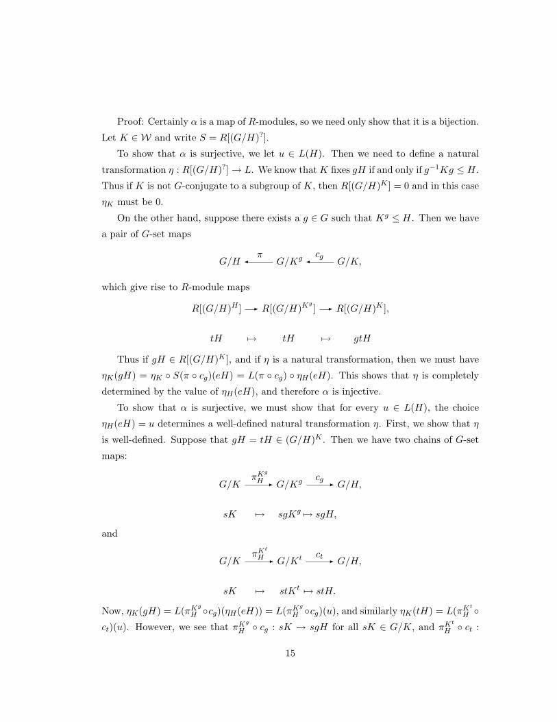
Finally we need to show that η is a natural transformation (i.e., that naturality

holds even for commutative squares that do not involve R[(G/H)H ]). Suppose that

f : G/J → G/K is a G-set map. We need the diagram in Figure 3.1 to commute:

R[(G/H)K ]S(f)- R[(G/H)J ]

L(K)

ηK

? L(f)- L(J)

ηJ

?

Figure 3.1: The natural transformation condition

If R[(G/H)K ] = 0 then the diagram commutes, so we assume that there exists some

gH ∈ (G/H)K . Then Kg ≤ H, and there is a G-set map p : G/K → G/H. Also, since

f : G/J → G/K is a G-set map, J t ≤ K for some t ∈ G, and J tg ≤ H. As before,

ηK(gH) = L(p)(u).

Now

(ηJ S(f))(gH) = ηJ(tgH)

= ηJ S(f) S(p)(eH)

= ηJ S(p f)(eH)

= L(p f) ηH(eH)

= L(p f)(u)

= L(f) L(p)(u)

= L(f) ηK(gH).

16

Proposition 3.7 R[(G/H)?] is projective in CSW(G) if H ∈ W.

Proof: Let θ : M → N be an epimorphism and η : R[(G/H)?] → N be a mor-

phism in CSW(G). Regard CSW(G) as mod-RW. Then by the proof of Proposition

2.1 in [54], each functor L becomes⊕

K∈W L(K) and every natural transformation α

becomes⊕

K∈W αK . In particular, the epimorphism θ is a surjective RW-map equal to⊕K∈W θK .

Since θ is a surjection there exists u ∈M(H) such that θ(u) = ηH(eH) ∈ N(H), and

since θK maps into N(K) for each K, it must be that u ∈M(H) and θH(u) = ηH(eH).

Now let φ : HomCSW (R[(G/H)?],M) → M(H) denote the R-module isomorphism

φ(ζ) = ζH(eH) for all η, guaranteed by the last proposition. Thus

φ−1(u) ∈ HomCSW (R[(G/H)?],M),

and

u = φ(φ−1(u))

= (φ−1(u))H(eH).

Thus we get

ηH(eH) = θH(u)

= θH(((φ−1(u))H)(eH))

= (θH (φ−1(u))H))(eH)

= (θ (φ−1(u))H(eH),

which implies as in Proposition 3.6 that η = θ φ−1(u). Thus R[(G/H)?] is projective.

We now define, for a G-CW complex Ω and a subposet X ⊆ S = S(G) such that Xis closed under conjugation, a chain complex C∗(Ω?) of objects in CSX (G). We define

Cn(Ω?) = R[Ω?n], where Ωn is the G-set of n-cells, and the boundary map dn : Cn(Ω?)→

Cn−1(Ω?) by the “obvious” natural transformation – for each H ∈ X and for all ω ∈ ΩH ,

we set

(dn)H(ω) = δn(ω),

17

where δn is the nth boundary homomorphism in the usual chain complex C∗(Ω;R). Note

that Cn(Ω?) is a complex of projective objects of CSS(G), since S = S(G) is the set of

all subgroups of G and therefore StabG(ω) ∈ S for all ω ∈ Ω.

Now let F be a Sylow p-subgroup of G. By the Note following the statement of

the Main Structure Theorem, F 6= 1. Also, let ∆ = Σ be the G-CW-complex in the

statement of Theorem 3.1, let S = S(F ) be the set of all subgroups of F , let V = S−1be the set of all nonidentity subgroups of F 6= 1, and let ∆S be the subcomplex of ∆

consisting of cells δ ∈ ∆ such that StabF (δ) ∈ V.

First, we note that F acts on ∆S : if 1 6= f ∈ StabF (δ) and h ∈ F then 1 6= hfh−1 ∈F and hfh−1(hδ) = hfδ = hδ, so StabF (hδ) 6= 1 for all δ ∈ ∆S , h ∈ F . Thus ∆S is an

F -subcomplex of ∆.

We get the usual short exact sequence of chain complexes:

0→ C∗(∆?S)→ C∗(∆?)→ C∗((∆,∆S)?)→ 0.

Apply ResVS to C∗(∆?S) to get a chain complex in CSV(F ). This complex is acyclic

if and only if for every X ∈ V, the complex C∗(∆XS ) obtained by evaluating at X is

acyclic. Let X ∈ V = S(F )− 1, or equivalently 1 6= X ≤ F .

Then

∆XS = σ ∈ ∆S |x · σ = σ, ∀x ∈ X

= σ ∈ ∆|StabF (σ) 6= 1, x · σ = σ, ∀x ∈ X

= σ ∈ ∆|1 6= StabF (σ) ≥ X

= σ ∈ ∆|StabF (σ) ≥ X 6= 1

= σ ∈ ∆|StabF (σ) ≥ X

= ∆X .

X is a nontrivial p-subgroup of G, and so to verify that C∗(∆?S) is acyclic we just

need to know that ∆P is R-acyclic for each nontrivial p-subgroup P of G, which is true

by the hypotheses on Σ in the statement of Theorem 3.1.

In addition C∗(∆?S) consists of projective objects of CSV(F ), because as F -sets

∆S,n∼=⊕k

i=1(F/Hi), and therefore as RV-modules R[(∆S,n)?] ∼=⊕k

i=1R[(F/Hi)?] is a

18

direct sum of projective modules since each δ ∈ ∆S,n has stabilizers in V. Thus if we

consider it as a complex of right RV-modules, then C∗(∆?S) is an acyclic complex of

projective modules, and therefore is a contractible complex.

This means that there are sn : ResSVCn → ResSVCn+1 such that (ResSVdn+1)sn +

sn−1ResSVdn = IdResCn= ResSVIdCn . We wish to show that this implies C∗(∆?

S) is a

contractible complex of RS-modules. Note that RV is a subalgebra of RS, so in general

RV-maps may not be RS-maps.

Since Cn(∆?S) ∼=

⊕R[(F/Hi)?] with Hi ∈ V, it suffices to assume Cn(∆?

S) =

R[(F/H)?] for some H ∈ V. Now for each H ∈ V ⊆ S, we have:

HomV(ResSVR[(F/H)?],ResSVT ) = HomV(R[(F/H)?],ResSVT )

∼= ResSVT (H) = T (H) ∼= HomS(R[(F/H)?], T )

and this isomorphism sends f 7→ ResSVf since the left-hand isomorphism sends (ResSVf)

to (ResSVf)H(eH) = fH(eH), which is the image under the right-hand isomorphism of

f . Thus for all H ∈ V and T ∈ CSS(F ),

ResSV : HomS(R[(F/H)?], T )→ HomV(ResSVR[(F/H)?],ResSVT )

is a bijection.

Surjectivity yields the existence of RS-maps tn : Cn → Cn+1 such that sn = ResSVtn.

Injectivity then implies ResSV(tn−1dn + dn+1tn) = ResSVIdn, and thus tn−1dn + dn+1tn =

Idn, so C∗(∆?S) is contractible in CSS(F ). Here we have also used the fact that ResSV is

additive on R[(F/H)?]; this is evident since Res is a forgetful functor. Finally, observe

that the collection sn is a chain map if tn is, since the boundary maps in the

complex ResSVC∗(∆?S) are by construction the images under ResSV of the boundary maps

of C∗(∆?S).

We now prove a lemma:

Lemma 3.8 Let 0→ E∗ → C∗ → P∗ → 0 be a short exact sequence of chain complexes,

where P∗ is a complex of projectives and E∗ is contractible. Then C∗ ∼= P∗ ⊕ E∗.

Proof: Let αn : En → En−1 and βn : Pn → Pn−1 be the differential maps on En and

Pn, let in : En → En ⊕ Pn and jn : Pn → En ⊕ Pn be the canonical inclusions, and let

qn : En ⊕ Pn → En and rn : En ⊕ Pn → Pn be the canonical projections.

19

In each degree we have a short exact sequence

0→ En → Cn → Pn → 0

and since Pn is projective, we may assume for each n that Cn ∼= En⊕Pn and the middle

maps are in and rn respectively. We should like the differential map dn on Cn to be

simply αn⊕βn, but in general this need not be true: the summands of Cn may be mapped

into each other. However, it is true that dn is well-behaved at least on the En summand:

that is, given x ∈ En and 0 = 0Pn , we have dn(x, 0) = dnin(x) = in−1αn(x) = (αn(x), 0).

We also know, given y ∈ Pn, that the Pn−1-entry of dn(0, y) is rn−1dnin(y) =

βnrnin(y) = βn(y). So the only difficulty is that Pn might map to En−1 in a nontrivial

way. This map Pn → En−1 is the composition φn := qn−1dnjn, so that dn(x, y) =

(αn(x) + φn(y), βn(y)).

Now we define φ′n = (−1)nφn. We wish to show that the collection φ′ of all the

φ′n is a chain map P∗ → E∗ of degree -1. We need to show αn−1φ′n = φ′n−1βn, or

equivalently αn−1φn = −φn−1βn. Since in−2 is a monomorphism, it is equivalent to

show in−2αn−1φn = −in−2φn−1βn. The proof is now a routine if slightly lengthy diagram

chase; it uses the fact that inclusion followed by projection is the identity, that squares of

boundary maps are zero, that the identity on a direct sum is the sum of the projections

followed by the inclusions, and the chain map condition.

Thus φ′ is a chain map of degree -1. Now the identity on E∗ is nullhomotopic, so

φ′ = IdE∗φ′ ' 0φ′ = 0 and φ′ is nullhomotopic.

Thus we have maps θn : Pn → En such that φ′n = θn−1βn + αn+1θn. Now let

θ′n = (−1)nθn, and define Θ : C∗ → E∗ ⊕ P∗ by Θ(x, y) = (x + θ′(y), y). Θ is then an

isomorphism of complexes with Θ−1(x, y) = (x− θ′(y), y). To show that Θ and Θ−1 are

chain maps amounts to showing that αθ′ = φ+ θ′β, or φ = αθ′− θ′β, and we know that

(−1)nφn = φ′n = αn+1θn + θn−1βn, so φn = αnθ′n − θ′n−1βn. This proves the lemma.

Thus C∗(∆?) ∼= E∗ ⊕ P∗ where E∗ = C∗(∆?S) is contractible and P∗ = C∗((∆,∆S)?)

in CSS(F ) is a complex of projectives.

Proposition 3.9 Evaluation of a coefficient system at a particular K (or F/K) is a

functor CSW(G)→ R[NG(H)/H]-mod, which: (1) respects direct sums, (2) sends pro-

jective objects to projective objects, and (3) sends contractible complexes to contractible

complexes.

20

Proof: Evaluation at K is a functor because the composition of natural transforma-

tions is defined by (θφ)K = θKφK , and it has values in R[NG(H)/H]-mod as observed

above. Let evK : CSW(G)→ R-mod be this functor.

To show (1) we could define the direct sum of two coefficient systems and show that it

satisfies the universal property of the direct sum. This is straightforward. Alternatively,

we can take direct sums in mod-RW, apply the explicit equivalence of categories s: mod-

RW → CSW(G) from ([30], Theorem 7.1, [54], 2.1), and evaluate at K. We choose to

use this second approach; the idea is that direct sums are very well-understood mod-

RW, while the evaluation functor is very well-understood in CSW(G). We will also

prove (2) and part of (3) this way.

Given K ∈ W and L,M ∈ mod-RW, the explicit formula in [30] and [54] tells us

that evK(s(L⊕M)) = (s(L⊕M)(K) is the R-module (L⊕M)IdK ∼= (LIdK)⊕M IdK),

which is exactly evK(s(L))⊕ evK(s(M)), as desired. Observe that we really get a right

R-module structure this way, but for us R is commutative so left modules and right

modules are the same.

(3) follows from (1), since a contractible complex (Cn, dn) has the form Cn ∼= An+1⊕Bn where dn|An = 0 and dn|Bn is an isomorphism Bn → An. Notice that evK sends zero

maps to zero maps and therefore sends complexes to complexes, because the 0 object is

sent to 0 by the same sort of argument as in the proof of (1).

To show (2), we note that projectives in both R-mod and mod-RW are summands

of free modules. By (1), evaluation respects direct sums, so it is enough to show that

evaluation sends free modules to free (or projective) modules; and by (1) again it is

enough to show that RW is sent to a free R-module by evaluation at K ∈ W.

As in (1), s(RW)(K) = RWIdK . As an R-module, this is generated by all α such

that α IdK is defined; by definition of the category algebra RW, it is therefore the

free R-module on all α which have domain K. We want to show that this is in fact

a free R[NG(K)/K]-module. As seen above, R[α|Dom(α) = K] = R[iKg≤J cg].NG(K)/K acts on the R-basis iKg≤J cg by nK (iKg≤J cg) = iKng≤Jn cng =

iKg≤Jn cng. This action is defined since Kng = (Kn)g = Kg ≤ J . Thus NG(K)/K

acts by permuting the symbols cg : K → Kg. This is a free action, which proves the

proposition.

21

So, continuing with the proof of the Main Structure Theorem, we take our isomor-

phism C∗(∆?) ∼= E∗ ⊕ P∗ of complexes in CSS(F ), and evaluate at K = 1 to get an

isomorphism of complexes of RF -modules: C∗(∆) ∼= P∗(1)⊕ E∗(1).

Now induce these complexes from F to G. In the previous paragraph we have

considered C∗(∆) as an RF -module. Properly, it is the RF -module ResGF C∗(∆) obtained

by taking the RG-module C∗(∆) and letting the subgroup F act. Thus we obtain

IndGFResGF C∗(∆) ∼= IndGFE∗(1) ⊕ IndGFP∗(1), and P ′∗ := IndGFP∗(1) is projective and

E′∗ := IndGFE∗(1) is contractible. Finally, C∗(∆) is a summand of IndGFResGF C∗(∆) by

c 7→∑

g∈G/F

g ⊗ g−1c, h⊗ c 7→ |G : F |−1hc, c ∈ C∗(∆), h ∈ G.

Therefore C∗(∆) is a summand of P ′∗⊕E′∗. If ∆ is a finite-dimensional CW-complex

then the Krull-Schmidt theorem (see for instance [55], 11.5 and 11.6) guarantees that

C∗(∆) ∼= Q∗ ⊕D∗ for some summands Q∗ of P ′∗ and D∗ of E′∗. Thus D∗ is contractible

and Q∗ is a complex of projectives, finishing the proof of Webb’s original theorem.

However, in the new case where our complex is bounded below but not necessarily

above, we need to convince ourselves that the Krull-Schmidt theorem still holds.

Definition 3.10 ([5], Definition A.1) An additive category C is called:

(i) ω-local if every object A ∈ C decomposes into a countable direct sum of objects

with local endomorphism rings;

(ii) fully additive if any idempotent morphism in C splits

(iii) locally finite (over S) if it is fully additive and HomC(A,B) is a finitely-

generated S-module for all objects A,B ∈ C.

(iv) Krull-Schmidt if every object has a unique decomposition into a direct sum of

objects which have local endomorphism rings.

Proposition 3.11 ([5], Proposition A.2) Suppose that S is a complete local noetherian

ring. If C is a locally-finite category over S, then both the category C(C) of chain

complexes of objects of C and the homotopy category K(C) are ω-local.

Proof: The proof appears in Appendix A of [5].

Theorem 3.12 Let G be a finite group and R a complete p-local ring. The category

C(RG)-mod of chain complexs of finitely-generated RG-modules is Krull-Schmidt.

22

We apply Proposition 3.11, taking S = R, and C to be the category of finitely-

generated RG-modules. We verify that the hypotheses of the above proposition are

satisfied. Clearly R is a complete local noetherian ring: it is either a field or a complete

discrete valuation ring, either of which is a complete local noetherian ring. We also

need C to be locally finite over R, which (by definition) means we need the following

two facts:

(1) Every idempotent morphism e : M →M for M in C splits, and (2) HomC(M,N)

is finitely generated over R for all M,N .

Condition (1) follows immediately from Fitting’s Lemma, which says (in particular)

that for any M ∈ C = RG-mod, any endomorphism f of M must satisfy M = Im(fm)⊕Ker(fm) for some m > 0. If we also assume f is idempotent, then we see that f must

split.

Condition (2) is clear if R = k is a field since a finitely-generated kG-module is a

finite-dimensional k-vector space as long as G is a finite group. More generally, suppose

G is a finite group and R is a complete p-local ring, and let M and N be finitely-

generated RG-modules. We want to show that HomRG(M,N) is a finitely-generated

R-module.

First, since G is a finite group, M and N are finitely-generated over R. Then since R

is a principal ideal domain, M ∼= Rr⊕R/(a1)⊕ . . .⊕R/(am) for some integers r,m ≥ 0

and some a1, . . . , am ∈ R, and similarly for N . Thus we may write an R-homomorphism

from M to N as an (r+m)× (r+m) matrix, so HomR(M,N) is finitely-generated over

R.

Finally, R is a noetherian ring, so a finitely-generated R-module is a noetherian

R-module. Thus HomR(M,N) is noetherian, so any R-submodule of HomR(M,N) is

finitely-generated over R. But HomRG(M,N) is an R-submodule of HomR(M,N), so

HomRG(M,N) is finitely-generated over R.

So if C = RG-mod then we have that that C(C) is ω-local, which is to say that every

object in C(C) decomposes into a direct sum of objects which have local endomorphism

rings. Of course, C(C) is not only additive but abelian (it has kernels, cokernels, and

a 0 object). Moreover, C(C) is equivalent to a small category if and only if C is. To

see that C is equivalent to a small category, we make two simple observations. First,

HomC(A,B) is small for all A and B. Second, C is equivalent to the category of all

23

representations, whose objects are group homomorphisms G→ GL(V ) for some finitely-

generated R-module V . Again, any finitely-generated V is a quotient of some Rn, and

the collection of quotients V of Rn such that n ≥ 0 is a set, as is then the collection of

group homomorphisms G→ GL(V ) for all such V .

Therefore, C(C) is equivalent by the Freyd-Mitchell full imbedding theorem (see

[29]) to a full subcategory of the category of T -modules for some ring T . Therefore by

Corollary 4.1.5 of [13], any decomposition of an object of C(C) into objects with local

endomorphism rings is unique up to isomorphism and reindexing. So in fact C(C) is

Krull-Schmidt, proving the theorem.

Corollary 3.13 Suppose G is a finite group and R is a complete p-local ring. Let

P∗ ⊕ E∗ =⊕

i∈IMi∗ be a direct-sum decomposition of P∗ ⊕ E∗ into indecomposable

complexes, where P∗ is a complex of projective RG-modules, E∗ is contractible, and P∗and E∗ are both bounded below. Then each M i

∗ is either a complex of projective modules

or is contractible.

Proof. By the Krull-Schmidt property, any indecomposable M i∗ in the decomposition

is isomorphic to a summand either of P∗ or of E∗.

This finishes the proof of part (i) of Theorem 3.1.

Finally, any summand of any direct sum decomposition of an object of C(C) will also

be an object in C(C), and will therefore (again by Proposition A.2 in [5]!) have a de-

composition into objects with local endomorphism rings. So in fact any indecomposable

summand must have a local endomorphism ring. (The converse is easy; a decomposable

summand has a non-local endomorphism ring, since we may write the identity as the

sum of two non-invertible projection maps). Therefore every object in C(C) decomposes

uniquely into indecomposables. This finishes part (ii) of Theorem 3.1.

Remark. The reader is invited to see [32] for an alternative treatment of the Krull-

Schmidt theorem in arbitrary categories.

Remark. Lemma 3.8, which is used in proving part (i) of Theorem 3.1, is a mod-

ification of a lemma used by Symonds in [47]. In our lemma, the complexes may be

unbounded. In Symonds’ lemma, the complexes must be bounded below. Both lemmas

therefore apply to the chain complex of a finite- or infinite-dimensional CW-complex.

24

Remark. Symonds has adapted this proof to prove a stronger claim, at least in the

case of a bounded CW-complex:

Theorem 3.14 ([45]) Let p be a prime, R a complete p-local ring, G a finite group,

and ∆ a bounded G-CW-complex. Suppose that the fixed point set ∆P is R-acyclic for

each p-subgroup P ≤ G that intersects H non-trivially. Let C∗(∆) denote the augmented

CW-chain complex of ∆ over R, considered as a complex of RG-modules.

Then C∗(∆) ∼= P∗ ⊕ E∗, where P∗ is a complex of trivial source RG-modules that

are projective relative to subgroups that have trivial intersection with H, and E∗ is split

exact.

Remark. Webb’s original theorem then follows by taking H = G.

Corollary 3.15 ([45]) Let Γ be a finite group and let ∆ = |Sp(Γ)|. Thus Aut(Γ) acts

on ∆ and also on C∗(∆).

Then C∗(∆) ∼= P∗⊕E∗ as a complex of RAut(Γ)-modules, where P∗ is a complex of

RAut(Γ)-modules which are projective on restriction to Γ (via the map Γ → Inn(Γ) ≤Aut(Γ)) and E∗ is split exact.

The Corollary ultimately comes from applying the Theorem with G = Aut(Γ) and

H = Inn(Γ). We do not use or prove these statements here, but the reader is invited to

see [45] for details.

25

Chapter 4

Alternative complexes

Let G be a finite group, and p a prime.

So far we have been working with the G-CW-complexes |Sp(G)|, |Ap(G)|, etc., which

are all G-homotopy-equivalent and which are all bounded. The reason for looking at

these complexes in the first place was that they generalized the building of a finite

group of Lie type in characteristic p. More precisely, if G is a finite group of Lie type

in characteristic p, then these complexes have homology only in one degree, where the

homology is the usual Steinberg module (Steinberg representation).

Bill Dwyer ([16], [17]) has found various other constructions of G-CW-complexes,

which all have the same homology as the subgroup complexes we have been considering,

but which may be unbounded. In fact Dwyer exhibits homology isomorphisms from

his infinite-dimensional complexes to |Sp(G)|. These are constructed as the nerves of

various G-categories.

We should like to know whether or not Dwyer’s “alternative” complexes are of the

same homotopy type as Sp(G). (Recall that we know that Sp(G), Ap(G), etc., all have

the same homotopy type.) If not, then these new unbounded complexes would be new

candidates for the title of “Steinberg complex.”

We now state the following general theorem.

Theorem 4.1 Let A∗ and B∗ be complexes of projective modules which are bounded

below, and suppose φ is a chain map A∗ → B∗ which induces isomorphism on homology.

Then φ is a homotopy equivalence.

26

Proof: Let C(φ) be the mapping cone of φ, so C(φ)n = An−1⊕Bn, with differential

dn : C(φ)n → C(φ)n−1 given by (an−1, bn) 7→ (−dAn−1(an−1), φn−1(an−1) + dBn (bn)).

We thus have a short exact sequence of complexes,

0→ B∗ → C(φ)→ A∗[−1]→ 0,

where A∗[−1] is the chain complex with entry An−1 in degree n, together with the

obvious differential maps. Then Hn+1(A∗[−1]) = Hn(A∗), and therefore we have a long

exact sequence:

. . .→ Hn+1(C(φ))→ Hn(A∗)→ HnB∗ → Hn(C(φ))→ . . . ,

and in fact the map Hn(A∗)→ Hn(B∗) is Hn(φ). (This last statement is Lemma 1.5.3

of [57].) Now since φ induces isomorphism on homology, we see that Hn(C(φ)) = 0

for all n. On the other hand, C(φ)n = An−1 ⊕ Bn is projective for all n, so C(φ)

is a complex of projectives which is acyclic and bounded below. Therefore C(φ) is

contractible. But C(φ) is contractible if and only if φ is a homotopy equivalence (see

for instance Proposition 2.8 in Chapter 3 of [3]).

Theorem 4.2 If J∗ is the (unique up to isomorphism) minimal summand of projectives

coming from any of Dwyer’s complexes, then it is homotopy-equivalent to the usual

Steinberg complex.

Proof: From each of his complexes, Dwyer exhibits a map to the p-subgroups com-

plex which induces homology isomorphism. (This map is induced by a functor from the

category whose nerve he takes for his complex.)

Let R be a complete p-local ring. Then upon composition with the RG-chain ho-

motopy equivalences J∗ ' XβC (this equivalence exists by part (i) of the Main Structure

Theorem) and C(Sp(G);R) ' St∗, we get a map φ : J∗ → St∗ between bounded-below

complexes of projectives, which induces isomorphism on homology. Thus J∗ and St∗ are

RG-chain homotopy-equivalent.

27

Chapter 5

Explicit calculations of a

Steinberg complex, part I

The next several sections are devoted to examining a particular Steinberg complex in

great detail. It does seem to be quite challenging to calculate Steinberg complexes in

general. Still, we should like to have some concrete examples at our disposal, and this

type of exploration has not appeared much in the literature on the topic to date. The

question becomes, which example should we try first?

The Steinberg complex is a complex of projective kG-modules, and one may ask

whether or not its homology groups must also be projective as kG-modules. It is now

known that the homology of the Steinberg complex need not always be projective. A

few examples of groups whose Steinberg complexes will exhibit non-projective homology

may be found in [49]. It is one of these examples that we should like to examine first.

Let Cn be the cyclic group of order n, and let G21 = C7 o C3 be the non-abelian

group of order 21. G21 may be realized as the subgroup of S7 generated by (1234567)

and (235)(476), since

(1234567)2 = (1357246) = (235)(476)(1234567)(253)(467).

Then let W = G21 o C3 = ((C7 o C3) × (C7 o C3) × (C7 o C3)) o C3, where the

complement C3 acts by permuting the copies of G21 cyclically. Thus

W = 〈(1234567), (235)(476),

28

(1, 8, 15)(2, 9, 16)(3, 10, 17)(4, 11, 18)(5, 12, 19)(6, 13, 20)(7, 14, 21)〉,

and W has order 3473 = 27783. We wish to determine the Steinberg complex for the

finite group W , at the prime p = 3, over the ring R = F3.

We start by finding B3(W ), the W -poset of nonidentity 3-subgroups H ≤ W sat-

isfying O3(NW (H)) = H. (Recall that for q a prime and G a finite group, Oq(G) is

the unique largest normal q-subgroup of a finite group, equal to the intersection of all

q-Sylow subgroups of G.)

There are only four W -conjugacy classes of such subgroups of W . To enumerate

these conjugacy classes we can restrict our attention to subgroups of a single Sylow 3-

subgroup of W , since the Sylow 3-subgroups are all W -conjugate by Sylow’s Theorem.

Let

S = ((C3 × 0)× (C3 × 0)× (C3 × 0))o C3, or

S = 〈(2, 3, 5)(4, 7, 6), (1, 8, 15)(2, 9, 16)(3, 10, 17)(4, 11, 18)(5, 12, 19)(6, 13, 20)(7, 14, 21)〉.

Then S has order 34 so S ∈ Syl3(W ). When it is clear that we are working inside S we

may identify ((C3 × 0)× (C3 × 0)× (C3 × 0))oC3 with (C3 ×C3 × C3)oC3. We also

let C denote the complement 0× 0× 0× C3.

Lemma 5.1 Let H ≤ S. If (a1, a2, a3, 0) ∈ H and ai 6= 0 for all i, then NW (H) =

NS(H).

Proof: S consists of exactly the elements of W which have 0 in all C7-components.

So we consider an arbitrary element normalizing H and show that it has no nonzero

C7-component.

Writing W as ((C7 o C3)× (C7 o C3)× (C7 o C3))o C3, we conjugate the element

h = (0, a1, 0, a2, 0, a3, 0) ∈ H ≤ S by t = (x1, y1, x2, y2, x3, y3, z). Then if φ : C3 →Aut(C7) is the homomorphism giving the semidirect product C7 oC3 described above,

we find that the ith G21-component of t ∗ h ∗ t−1 is (operations in subscripts are carried

29

out mod 3):

(xi, yi) ∗ (0, ai−z) ∗ (xi, yi)−1 = (xi + φ(yi)(0), yi + ai−z) ∗ (φ(−yi)(−xi),−yi)

= (xi + φ(yi + ai−z)(φ(−yi)(−xi)), yi + ai−z − yi)

= (xi + (φ(yi + ai−z) φ(−yi))(−xi), ai−z)

= (xi + φ(yi + ai−z − yi)(−xi), ai−z)

= (xi + φ(ai−z)(−xi), ai−z)

So if t ∗ h ∗ t−1 ∈ H ≤ S, then −xi = φ(ai−z)(−xi), which is true if and only if

ai−z = 0 or xi = 0. Since ai−z 6= 0 by assumption, this yields xi = 0, and NW (H) ⊆ S.

Corollary 5.2 Let H ≤ S. If (a1, a2, a3, 0) ∈ H and i 6= 0 for all i, then

O3(NW (H)) = NS(H).

Proof: By Lemma 1.1, NW (H) = NS(H), so NW (H) ≤ S. Therefore NW (H) =

NS(H) is a 3-group, and equal to its 3-core.

Proposition 5.3 Any nonidentity subgroup H ≤ S satisfying O3(NW (H)) = H is

W -conjugate either to: (i) S, (ii) C, or (iii) a subgroup of C3 × C3 × C3 × 0.

Proof: Write C3 additively as 0, 1, 2, and write S = C3 × C3 × C3 o C3. Now

let H ≤ S such that O3(NW (H)) = H, and assume that H is not a subgroup of

C3 × C3 × C3 × 0. That is, the restriction to H of the canonical projection π : S → C

is surjective. If this map H → C is an isomorphism, then H = 〈h〉 is cyclic of order 3.

Then the first three components (the non-C components) of h sum to 0. In this case,

H = 〈h〉 is conjugate to C: assume without loss of generality that h has C-component

equal to 1, and write h = (a, b,−a− b, 1). Then

(a, 0,−b, 1)(a, b,−a− b, 1)(0, b,−a, 2) = (a− a− b, 0 + a,−b+ b, 2)(0, b,−a, 2)

= (−b, a, 0, 2)(0, b,−a, 2) = (−b+ b, a− a, 0 + 0, 1) = (0, 0, 0, 1),

30

so h is conjugate to the generator of C, and 〈h〉 is conjugate to C.

So we assume that H → C has a nontrivial kernel, K. K must have order 3,9, or

27. If |K| = 27, then H = S and we are done.

First suppose |K| = 3, so that |H| = 9 and H is abelian. In particular every element

of H centralizes every element of K. We know we have nonidentity elements k, h ∈ Hsuch that π(k) = 0, π(h) = 1, so k = (a, b, c, 0) and h = (t, u, v, 1). Since h centralizes

k, we calculate that k = (a, a, a, 0) with a ∈ 1, 2. From this, Corollary 5.2 yields that

O3(NW (H)) = NS(H).

Now, either H ∼= C9 or H ∼= C3 × C3. If H is not cyclic, then H is generated

by k = (a, a, a, 0) and h = (t, u, v, 1), both of order 3. Thus h = (t, t, t, 1). Hence

H is generated by (1, 1, 1, 0) and (0, 0, 0, 1), so H = ∆(C3) × C3, where ∆(C3) is the

diagonally-embedded subgroup 〈(1, 1, 1)〉 of C3 × C3 × C3. But now direct calculation

on the generators shows that (1, 2, 0, 0) ∈ NS(H) − H, and therefore H 6= NS(H) =

O3(NW (H)).

On the other hand, suppose that H is cyclic, so H ∼= C9. In this case H =

〈(t, u, v, 1)〉, with t + u + v 6= 0 (again, (1, 1, 1, 0) ∈ K ≤ H). Once again it turns

out that we have (1, 2, 0, 0) ∈ NS(H)−H so once again O3(NW (H)) 6= H.

So finally we assume that |K| = 9, and |H| = 27. In particular, H is a maximal

subgroup of S. This shows (see 5.2.4 in [34], p.130) that H / S, so O3(NS(H)) =

NS(H) = S 6= H. We wish to show, therefore, that NW (H) = NS(H). We should like

to show (1, 1, 1, 0) ∈ H, since then Lemma 1.1 would finish the proof. For this, it suffices

to show that (1, 1, 1, 0) is an element of the Frattini subgroup F = Frat(S), since F is

the intersection of all maximal subgroups of S.

Since S is a 3-group, the Burnside Basis Theorem ([34], 5.3.2, p.140) states that

F = S′S3. So we need only exhibit a factorization of (1, 1, 1, 0) as the product of an

element of S′ and an element of S3. But we already know that, for instance, (1, 1, 1, 0) =

(1, 0, 0, 1)3.

Theorem 5.4 The nonidentity subgroups H ≤W which satisfies O3(NW (H)) = H are

exactly the W -conjugates of: (i) S, (ii) C, (iii) C3× 0× 0× 0, and (iv) C3×C3× 0× 0.

Proof: The 3-subgroups H ≤ W are W -conjugate to subgroups of S, by Sylow’s

Theorem, so the only candidates are those listed in Proposition 5.3. By Corollary 5.2,

31

O3(NW (S)) = S (and by Lemma 1.1, NW (S) = NS(S) = S; later we shall want this

fact as well). To show (ii), we let x = (0, 0, 0, 0, 0, 0, 1) ∈ C, so C = 〈x〉. Then

NW (C) =a ∈W |a−1xa ∈ x, x2

However, given a = (x1, y1, x2, y2, x3, y3, z) ∈ W , we have a−1xa = x2 ⇔ xa = ax2 ⇔(0, 0, 0, 0, 0, 0, 1)(x1, y1, x2, y2, x3, y3, z) = (x1, y1, x2, y2, x3, y3, z)(0, 0, 0, 0, 0, 0, 2) ⇒ 1 +

z = z + 2, which is impossible. Thus

NW (C) =a ∈W |a−1xa = x

But let a ∈ W . Then a−1xa = x ⇔ xa = ax ⇔ xax−1 = a ⇔ a ∈ ∆(G21) × C3, so

NW (C) = ∆(G21)× C3.

Now, C is certainly a normal 3-subgroup of NW (C), of order 3. The Sylow 3-

subgroups of ∆(G21)× C3 have order 9, but there are more than one of these: there is

one for each of the Sylow 3-subgroups of G21, and there are exactly 7 of these. Thus

the Sylow 3-subgroups of NW (C) are not normal, and so the largest normal 3-subgroup

of NW (C) is C, verifying (ii).

It remains to show that every nonidentity subgroup H ≤ C3×C3×C3×0 satisfying

O3(NW (H)) = H is W -conjugate either to C3 × 0 × 0 × 0 or to C3 × C3 × 0 × 0. Let

D denote C3 × C3 × C3. By Corollary 5.2, D / S implies O3(NW (D)) = S 6= D. So a

nonidentity subgroup H ≤ D satisfying O3(NW (H)) = H must have order either 3 or

9.

There are 27− 1 = 26 elements of D of order 3, so there are 26/2 = 13 subgroups of

D of order 3. We can also count the subgroups of D of order 9: If we wish to construct

such a subgroup, we can choose a generator in any of 27 − 1 = 26 ways, then choose

another generator in any of 27 − 3 = 24 ways to get a subgroup of order 9. But given

the first generator, 9 − 3 = 6 distinct choices for the second generator will yield the

same subgroup. This means that every nonidentity element of D is contained in exactly

24/6 = 4 subgroups of D of order 9. Now the total number of subgroups of order 9

is the number of nonidentity elements of D, times the number of order-9 subgroups

containing a given nonidentity element, divided by the number of nonidentity elements

in each order-9 subgroup, or 26 ∗ 4/8 = 13. So there are 13 order-3 subgroups and 13

32

order-9 subgroups. (See also [36], where the identity

m∑λ=0

(−1)λp(λ2)Eλ(G) = 0

is proven for G an arbitrary p-group: here |G| = pm, and Eλ(G) denotes the number of

elementary abelian subgroups of G of size pλ. This work is also cited in [37].)

Omitting parentheses and commas, the order-9 subgroups are generated by

(110, 001), (010, 001), (100, 001), (210, 001), (100, 021), (100, 010), (010, 201),

(010, 101), (110, 201), (100, 011), (210, 201), (210, 101), and (110, 101).

Except for 〈010, 001〉, 〈100, 001〉, and 〈100, 010〉, all of these subgroups satisfy the

hypotheses of Corollary 5.2, so for these groups the fact that D is abelian yields

O3(NW (H)) = NS(H) ≥ D H. The remaining order-9 subgroups are visibly W -

conjugate (actually S-conjugate) to 〈100, 010〉 = C3 × C3 × 0. Let H denote this

subgroup. We have D ≤ NW (H), and we see that 0 × 0 × G21 × 0 ≤ NW (H), so

C3×C3×G21× 0 ≤ NW (H). Following the calculation in the proof of Lemma 1.1, and

letting (a1, a2, a3) = (1, 1, 0) ∈ H, we see that if t = (x1, . . . , y3, z) ∈ W normalizes H,

then for each i, either xi = 0 or ai−z = 0. So taking z = 0 for the moment, we see that

NW (H)⋂G21×G21×G21 = C3×C3×G21. Suppose on the other hand that z = 1, so

that x2 = 0, x3 = 0 (since a2−1 6= 0, a3−1 6= 0). Then

NW (H) 3 t2 = (x1, y1, 0, y2, 0, y3, 1)2

= ((x1, y1) ∗ (0, y3), (0, y2) ∗ (x1, y1), (0, y3) ∗ (0, y2), 1 + 1)

= ((x1 + φ(y1)(0), y1 + y3), (0 + φ(y2)(x1), y2 + y1),

(0 + φ(y3)(0), y3 + y2), 2)

= ((x1, y1 + y3), (φ(y2)(x1), y2 + y1), (0, y3 + y2), 2).

This time, since a3−2 6= 0, a1−2 6= 0, the first C7-coordinate of t2 must be zero. But that

says exactly that x1 = 0, so we see that xi = 0 for all i. Hence any element of NW (H)

with nonzero C-coordinate must be an element of S. But we know that D ≤ NW (H),

so if there is any element t ∈ NW (H) with nonzero C-coordinate, then C ≤ NW (H).

33

But we can see that C does not normalize H. Thus NW (H) = C3 × C3 ×G21. Finally

O3(NW (H)) must have order at most 9, since NW (H) has non-normal (non-unique)

Sylow 3-subgroups of order 27, but H is a normal 3-subgroup of its normalizer, of order

9. Thus O3(NW (H)) = H, as claimed.

We are now reduced to showing that the order-3 subgroups of D which belong to

B3(W ) are W -conjugate to C3×0×0. The order-3 subgroups are generated, respectively,

by

100, 010, 110, 120, 001, 101, 201, 011, 012, 111, 112, 121, and 211.

Of these, those generated by 111, 112, 121, and 211 have, by Corollary 1.2, O3(NW (H)) =

NS(H) ≥ D H, since D is abelian. The remaining subgroups of D visibly fall into at

most 3 W -conjugacy classes. We consider a subgroup from each conjugacy class.

First let H = 〈(1, 1, 0)〉 ≤ D. We copy the work we did in showing that NW (C3 ×C3×0) ≤ C3×C3×G21 to show that NW (H) ≤ C3×C3×G21, since to eliminate other

elements we only considered their effect on the element (1, 1, 0). Direct calculation then

shows that NW (H) = C3 × C3 × G21. But we saw above that O3(C3 × C3 × G21 =

C3×C3×0 6= H. The same work also suffices to show thatNW (〈(1, 2, 0)〉) = C3×C3×0 6=(〈(1, 2, 0)〉, since all we used about the element (1, 1, 0) was that it was nonzero in the

first two components.

Finally let H = C3 × 0× 0 = 〈(1, 0, 0)〉 ≤ D. We claim that NW (H) = C3 ×G21 ×G21 × 0. First we assume for contradiction that t = (x1, . . . , y3, 1) ∈ NW (H). We

calculate that t−1 = ((x2, y2)−1, (x3, y3)−1, (x1, y1)−1), 2), so the first G21-component of

t ∗ (0, 1, 0, 0, 0, 0, 0) ∗ t−1 is (x1, y1) ∗ (x1, y1)−1 = (0, 0). Since we have assumed that

t ∈ NW (H), we see that conjugation by t sends a generator of H to zero, a contradiction.

So NW (H) ≤ G21 ×G21 ×G21. We can see directly that C3 ×G21 ×G21 ≤ NW (H), so

NW (H) is either G21 × G21 × G21 or C3 × G21 × G21. But we see that a generator of

C7 × 0× 0 does not normalize H. Thus NW (H) = C3 ×G21 ×G21. However,

O3(NW (H)) =⋂

P∈Syl3(NW (H))

P

= C3 × (⋂

Q∈Syl3(G21)

Q)× (⋂

R∈Syl3(G21)

R)

= C3 × 0× 0.

34

Chapter 6

Explicit calculations of a

Steinberg complex, part II

As in the last section, let W = G21 o C3, where G21 is up to isomorphism the unique

non-abelian group of order 21, and let p = 3. We continue to find information about

the Steinberg complex of W at p = 3 over the ring R = F3.

Let us choose one representative from each of the four conjugacy classes of subgroups

appearing in B3(W ) and give them all names: We have S = C3 × C3 × C3 o C3 and

C = 0× 0× 0× C3. Now let A denote C3 × C3 × 0× 0 and B denote C3 × 0× 0× 0.

We have chosen our representatives in such a way that B ⊆ A ⊆ S and C ⊆ S. In

fact this is the full list of inclusions possible:

Proposition 6.1 No conjugate of C is a subgroup of any conjugate of A.

This says that no other set of representatives would have yielded a larger set of

inclusions of subgroups, since by cardinality this is the only candidate for an additional

inclusion.

Proof: Suppose gC ⊆ hA for some g, h ∈ W ; this would yield xC ⊆ A for some

x ∈ W . But this is impossible; direct computation shows that the C-component of an

element of W is never changed by conjugation.

In particular, C and B are not conjugate, so we have a minimal list of representatives

of B3.

35

Proposition 6.2 The W -stabilizer of a simplex σ = (H0 ≤ . . . ≤ Hn) is⋂ni=0NW (Hi).

Proof: By induction on n. The stabilizer of a vertex H0 is g ∈ W |gHg−1 = H =

NW (H). If n ≥ 1, then the stabilizer of H0 ≤ . . . ≤ Hn is g ∈ W |gHig−1 = Hi∀i =

g ∈ W |gHig−1 = Hi, 0 ≤ i ≤ n − 1 ∩ g ∈ W |gHng

−1 = Hn = (⋂n−1i=0 NW (Hi)) ∩

NW (Hn) = (⋂ni=0NW (Hi)).

We have in the previous section computed the normalizers of the various subgroups

(up to conjugacy) in the G-poset B3(W ). This together with the last proposition allows

us to compute the stabilizer of each of our simplices:

NW (S) = S

NW (C) = ∆(G21)× C3

NW (B) = C3 ×G21 ×G21 × 0

NW (A) = C3 × C3 ×G21 × 0

StabW (C ≤ S) = ∆(C3)× C3

StabW (B ≤ A) = C3 × C3 ×G21 × 0

StabW (B ≤ S) = C3 × C3 × C3 × 0

StabW (A ≤ S) = C3 × C3 × C3 × 0

StabW (B ≤ A ≤ S) = C3 × C3 × C3

We now calculate the size of the W -orbits of the simplices in our list, using the fact

that |Wσ| = |W : StabW (σ)|:

36

|W : StabW (S)| = 73

|W : StabW (C)| = 32 ∗ 72

|W : StabW (B)| = 3 ∗ 7

|W : StabW (A)| = 3 ∗ 72

|W : StabW (C ≤ S)| = 32 ∗ 73

|W : StabW (B ≤ A)| = 3 ∗ 72

|W : StabW (B ≤ S)| = 3 ∗ 73

|W : StabW (A ≤ S)| = 3 ∗ 73

|W : StabW (B ≤ A ≤ S)| = 3 ∗ 73

We saw in the previous section that S includes exactly three subgroups conjugate to

A, and three subgroups conjugate to B. Each A contains two of the subgroups conjugate

to B, and there are 73 = 343 subgroups conjugate to S. Thus there are 73 ∗3∗2 = 2058

2-simplices in |B3(W )|. Each orbit of 2-simplices has size 3 ∗ 73, so there are exactly 2

orbits of 2-simplices. In fact there are 2 orbits of simplices of the form yB ≤ xA, since

no element will simultaneously send C3× 0× 0× 0 to 0×C3× 0× 0 and C3×C3× 0× 0

to C3 × C3 × 0× 0.

Continuing in this way, S contains 3 subgroups conjugate to A, so there are 3 ∗ 73

1-simplices of the form yA ≤ xS, and the orbit of S ≤ A has size 3 ∗ 73, so there is only

one orbit of 1-simplices of this form. Similarly there is only one orbit of simplices of the

form yB ≤ xS. It remains to determine the number of orbits of simplices of the formyC ≤ xS.

As we stated before, any conjugate of C will have a nontrivial C-component. Any

subgroup of S of order 3 that has nontrivial C-component must have generator (t, u, v, 1)

with t+u+v = 0. There are 3∗3∗1 = 9 choices for such triples (t, u, v) = (t, u,−t−u). All

of these give subgroups of S conjugate to C: given (t, u,−t−u, 1) ∈ S, (t, u,−t−u, 1) =

(0, u,−t, 0)(0, 0, 0, 1)(0,−u, t, 0). So there are 32 ∗ 73 1-simplices of the form xC ≤ yS,

and every orbit of such simplices has size 32 ∗ 73. So there is exactly one such orbit.

We can also say, therefore, that each conjugate of C is contained in exactly |W :

37

StabW (C ≤ S)|/|W : StabW (C)| = 32 ∗ 73/(32 ∗ 72) = 7 conjugates of S. Similarly each

conjugate of B is contained in 3 ∗ 73/(3 ∗ 7) = 72 conjugates of S and is contained in 14

conjugates of A.

The orbit complex |B3(W )|/W thus has 4 vertices (S,C,B,A), 5 1-simplices (C ≤S,B ≤ S,A ≤ S,B ≤ A, cB ≤ A), and 2 2-simplices (B ≤ A ≤ S, cB ≤ A ≤ S). The

orbit complex is homotopy equivalent to the cone over the wedge of a 0-sphere and a

1-sphere, which is contractible.

In fact it is always true that the orbit complex will be contractible:

Theorem 6.3 (Webb’s Conjecture.) Given any finite group G and prime p dividing

|G|, the orbit complex |Sp(G)|/G (or |Ap(G)|/G, |Bp(G)|/G, etc.) is contractible.

Proof: See [45].

Remark: Suppose G is a group whose order is divisible by a prime q. Then it is

clear that every Sylow q-subgroup of G lies in Bq(G) If the Sylow q-subgroups are the

only elements of Bq(G), then |Bq(G)|/G = Q is a single vertex since all the Sylow

p-subgroups are conjugate. On the other hand, suppose that Sylq(G) ( Bq(G). One

might think, since every q-subgroup of G is contained in some Sylow q-subgroup and

the Sylow q-subgroups are all conjugate, that |Bq(G)|/G must always be the cone over

the space |Bq(G)− Sylq(G)|/G. This would immediately prove Webb’s conjecture, but

in fact this argument will fail in general. As we have already seen in the example of

B3(W ) at hand, a pair of vertices in the orbit complex may be connected by multiple

edges. In particular, if Q is the vertex of the orbit complex which represents the Sylow

q-subgroups of G, then Q and another vertex may be connected in the orbit complex by

multiple edges, which cannot happen in the cone over |Bq(G)−Sylq(G)|. This situation

occurs if there is a Sylow q-subgroup Q with two subgroups X,Y ∈ Bq(G) such that X

is G-conjugate to Y but not NG(Q)-conjugate to Y .

38

Chapter 7

Explicit calculations of a

Steinberg complex, part III

As in the previous sections, let W = G21 o C3, where G21 is up to isomorphism the

unique non-abelian group of order 21, and let p = 3. We continue to find information

about the Steinberg complex of W at p = 3 over the ring R = F3.

Let ∆ = |B3(W )| and let k = F3. As a complex of vector spaces over k, we calculated

in the last section that the chain complex C∗(∆; k) is

0→(k3∗73 ⊕ k3∗73)→ (

k3∗73 ⊕ k3∗73 ⊕ k3∗72 ⊕ k3∗72 ⊕ k32∗73)→(k73 ⊕ k32∗72 ⊕ k3∗7 ⊕ k3∗72)→ k → 0,

where the nonzero terms are in dimensions 2, 1, 0, and −1.

Now let U be a small open neighborhood of M in ∆, where M the subspace of ∆

obtained by removing all vertices in the W -orbit of the vertex C, and removing all edges

in the orbit of the edge C ≤ S. Let V be a small neighborhood of the subspace of ∆

consisting only of the vertices in the orbits of C and S and the edges in the orbit of

C ≤ S. Then U ∪ V = ∆, and U ∩ V is homotopy-equivalent to the discrete space with

one vertex for each conjugate of S. This discrete space may be described as∨342i=1 S

0,

the bouquet of 342 copies of the 0-sphere, since the 0-sphere is a discrete space with

two points. Thus:

39

Proposition 7.1 We have a Mayer-Vietoris exact sequence:

0→ H2(U ∩ V )→ H2(U)⊕ H2(V )→ H2(∆)

→ H1(U ∩ V )→ H1(U)⊕ H1(V )→ H1(∆)

→ H0(U ∩ V )→ H0(U)⊕ H0(∆)→ 0.

On simplification, the sequence from Proposition 7.1 becomes:

0→ 0→ H2(U)⊕ 0→ H2(∆)

→ 0→ H1(U)⊕ H1(V )→ H1(∆)

→ k342 → H0(U)⊕ H0(V )→ H0(∆)→ 0.

In particular:

Corollary 7.2 H2(∆) ∼= H2(U) as vector spaces.

U has all the 2-simplices of ∆. These are, as we have seen, of the form xB ≤ yA ≤ zS,

for some x, y, z ∈ G. The subgroup S contains exactly 3 conjugates of A and 3 conjugates

of B. Each of these conjugates of A contains 2 conjugates of B, and each conjugate of

B is contained in 14 conjuates of A, of which exactly 2 are contained in S. So each

conjugate of S is a vertex of exactly 3 ∗ 2 = 6 2-simplices, as we have seen. These

2-simplices adjoin each other to form a hexagon whose center is S and whose outer

vertices are alternately conjugate either to A or B. Of course the complex is locally

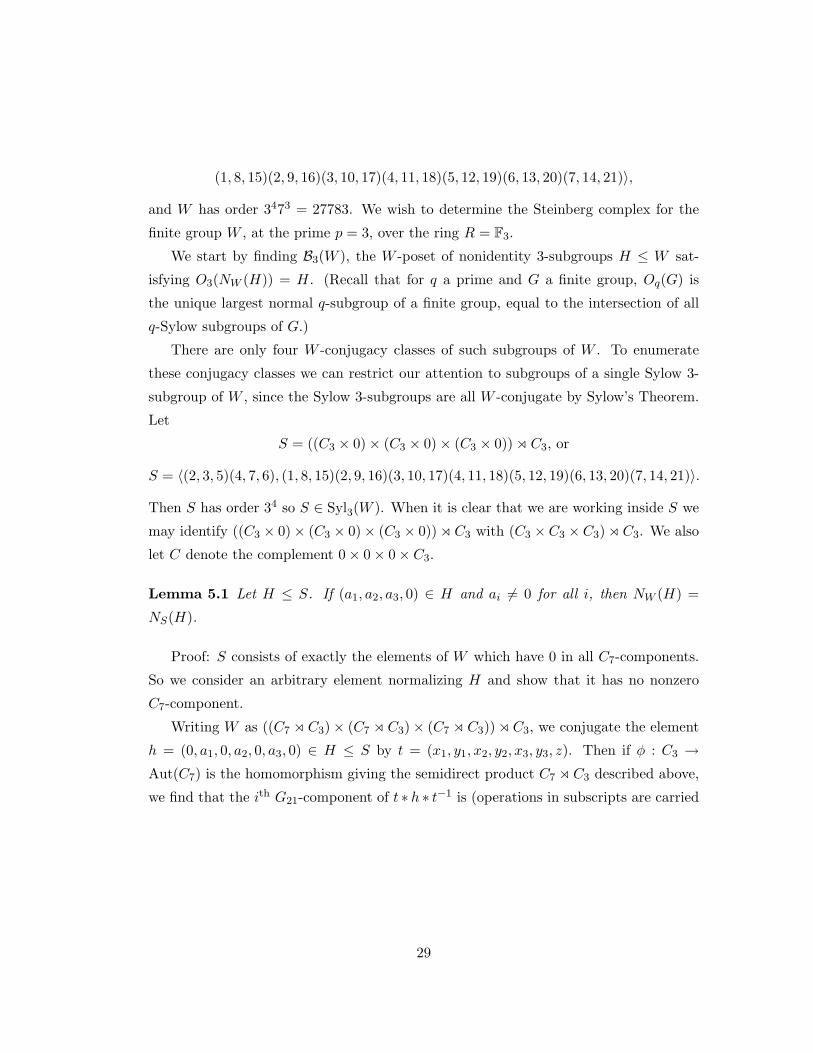
the same near every conjugate of S. We illustrate this in Figure 7.1. The labels on

the vertices are not technically correct; where it says A,B, or S, it really shows some

conjugate of that subgroup.

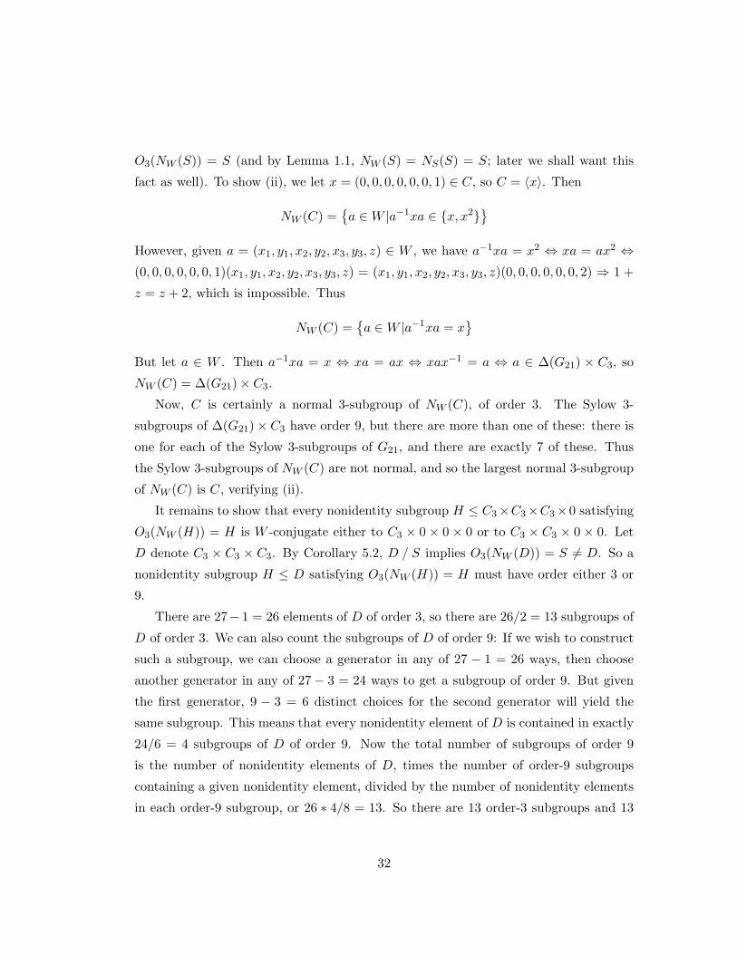
Now, we imagine “deforming” simultaneously all of these hexagons in U so that they

all look like triangles, or barycentrically subdivided triangles, with a conjugate of S in

the center of each triangle, a conjugate of A in the center of each edge, and a conjugate

of B at each vertex, as shown in Figure 7.2.

Relabeling our picture, we get a homotopy-equivalent CW-complex with 3 ∗ 7 = 21

vertices (one for each conjugate of B), 3 ∗ 72 = 147 edges (one for each conjugate of

40

S

B A

B

AB

A

Figure 7.1: A local view of a subspace U of |B3(W )|, near a Sylow 3-subgroup S of W

SB

B

A

B

A

A

Figure 7.2: A local view of the subspace U of |B3(W )|, with edges deformed

A), and 73 = 343 2-cells (one for each conjugate of S), whose barycentric subdivision

is our complex ∆. In this new complex E, two vertices are attached by an edge if and

only if their corresponding subgroups (which are conjugate to B) are contained in the

same conjugate of A. Each conjugate of B was contained in 14 conjugates of A, so in

E each vertex is an endpoint for 14 edges; equivalently, each vertex of E neighbors 14

other vertices.

Proposition 7.3 Let xB and yB be two distinct conjugates of B which do not neighbor

B in E. Then xB and yB do not border each other in E.

Proof: By computer.

Corollary 7.4 The vertices of E are partitioned into three sets, each of which has no

pair of vertices with an edge between them. That is, the vertices and edges of E form a

41

tripartite graph. In fact, the vertices and edges of E form the complete tripartite graph

K7,7,7.

Proof: Each of the 21 vertices of E has 14 neighbors, so each of the vertices of E

has 6 other vertices which it does not neighbor, and which do not neighbor each other

by Proposition 7.3. But this partite set cannot be any bigger than 7 vertices, since each

vertex in this partite set neighbors all the remaining 14 vertices.

The graphK7,7,7 has 73 3-cycles, and each 2-cell of E describes a 3-cycle in its vertices

and edges, so E is completely described as having the vertices and edges of K7,7,7 as

well as a 2-cell for every 3-cycle of K7,7,7. This complex is alternatively described as the

join of a 7-vertex discrete space with itself three times. Thus we have proven:

Theorem 7.5 U is homotopy equivalent to

(6∨i=1

S0) ? (6∨i=1

S0) ? (6∨i=1

S0).

Corollary 7.6 H2(∆; k) ∼= k216.

Proof:

U ' E

' (6∨i=1

S0) ? (6∨i=1

S0) ? (6∨i=1

S0)

'63∨i=1

S2.

Thus

H2(∆) ∼= H2(U)

∼= H2(∨216i=1S

2)

∼= k216.

42

Chapter 8

Explicit calculations of a

Steinberg complex, part IV

As in the previous sections, let W = G21 o C3, where G21 is up to isomorphism the

unique non-abelian group of order 21, and let p = 3. We continue to find information

about the Steinberg complex of W at p = 3 over the ring R = F3.

Proposition 8.1 Let k be a field which is algebraically closed of characteristic 3. There

are exactly eleven isomorphism classes of simple kG-modules: the trivial module, two of

dimension 9, six of dimension 27, and two of dimension 81.

Proof: By computer calculation, run in the program GAP (Groups, Algebras and

Permutations):

gap> new;Group([ (1,8,15)(2,9,16)(3,10,17)(4,11,18)(5,12,19)(6,13,20)(7,14,21),(2,3,5)(4,7,6)(8,9,10,11,12,13,14)(15,21,20,19,18,17,16) ])gap> Size(new);27783gap> tbl:=BrauerTable(new,3);BrauerTable( Group([(1,8,15)(2,9,16)(3,10,17)(4,11,18)(5,12,19)(6,13,20)(7,14,21),(2,3,5)(4,7,6)(8,9,10,11,12,13,14)(15,21,20,19,18,17,16) ]), 3 )gap> Display(tbl);CT1mod3

43

3 4 . . 2 1 2 1 1 1 1 17 3 3 3 3 3 3 3 3 3 3 3

1a 7a 7b 7c 7d 7e 7f 7g 7h 7i 7j2P 1a 7a 7b 7c 7d 7e 7f 7g 7h 7i 7j3P 1a 7b 7a 7e 7f 7c 7d 7j 7i 7h 7g5P 1a 7b 7a 7e 7f 7c 7d 7j 7i 7h 7g7P 1a 1a 1a 1a 1a 1a 1a 1a 1a 1a 1a11P 1a 7a 7b 7c 7d 7e 7f 7g 7h 7i 7j13P 1a 7b 7a 7e 7f 7c 7d 7j 7i 7h 7g17P 1a 7b 7a 7e 7f 7c 7d 7j 7i 7h 7g19P 1a 7b 7a 7e 7f 7c 7d 7j 7i 7h 7g

X.1 1 1 1 1 1 1 1 1 1 1 1X.2 9 A /A E 2 /E 2 J N /N /JX.3 9 /A A /E 2 E 2 /J /N N JX.4 27 -1 -1 6 I 6 /I -1 6 6 -1X.5 27 -1 -1 6 /I 6 I -1 6 6 -1X.6 27 B /B F -1 /F -1 K L /L /KX.7 27 /B B /F -1 F -1 /K /L L KX.8 27 C /C G 6 /G 6 L B /B /LX.9 27 /C C /G 6 G 6 /L /B B LX.10 81 D /D H -3 /H -3 M O /O /MX.11 81 /D D /H -3 H -3 /M /O O M

Remark: The characters come in Galois-conjugate pairs. Over F3, which is not

algebraically closed, it turns out that each nontrivial irreducible module is made up of

one of these pairs of modules. Thus over F3, up to isomorphism there is one simple

module of dimension 18, three of dimension 54, and one of dimension 162. Over the

field of 9 elements, each of these modules decomposes into a direct sum of two absolutely

irreducible modules.

Lemma 8.2 W has a normal 3-complement of size 73 = 343.

Proof: |W | = 34 ∗ 73, so a Sylow 7-subgroup of W has size 73 = 343. By Sylow’s

Theorem, the number of Sylow 7-subgroups of W divides the W -index of a Sylow 7-

subgroup, and is congruent to 1 mod 7. The index is 34 = 81, and 1 is the only divisor

44

of 81 which is congruent to 1 mod 7. Thus W has a unique Sylow 7-subgroup, which is

therefore normal in W .

Corollary 8.3 Each indecomposable projective kW -module P is isomorphic to the pro-

jective cover PU of a unique (up to isomorphism) simple module U . For each simple U ,

PU has composition factors U with multiplicity dim PU/dimU . In particular, if U and

T are simple kW -modules and U T , then Hom(PU , PT ) = 0.

Proof: This is part of Theorem 8.10 in [55].

Proposition 8.4 Let k be algebraically closed of characteristic 3. Then every indecom-

posable projective kW -module has k-dimension 81.

Proof: We have the following identity (see [55], 8.3), where the sum is taken over a

complete set of representatives of isomorphism classes of simple modules:

|W | =∑

U simple

(dim PU ∗ dim U),

and 81 = |W |3 divides dim PU for all U . If∑U

|W |3 ∗ dim U = |W |,

then it follows that dim PU = |G|3 for all U . We have one simple U of dimension 1, two

of dimension 9, six of dimension 27, and two of dimension 81. This gives us

81 ∗ (1 + 2 ∗ 9 + 6 ∗ 27 + 2 ∗ 81) = 81 ∗ (343) = |W |.

So dim PU = 81 for all U .

Corollary 8.5 Let k be an algebraically closed field of characteristic 3, and let S ∈Syl3(W ). For every simple module kW -module U , the restricted module (PU ) ↓S∼= kS.

Proof: PU is a projective kW -module, which implies (see [55], 8.2) that (PU ) ↓S is

a projective kS-module. Every finitely-generated projective kS-module is free (see [55],

8.1), so a projective kS-module of k-dimension 81 is isomorphic to kS.

45

Definition 8.6 Let R be a commutative ring with identity, G a finite group, H ≤ G,

and V an RG- module. We define the set function NormRH : V → V by

v 7→∑g∈H

(g · v).

Remark: We will often write NormH or Norm to mean NormRH if there is no chance

of confusion.

Remark: Norm is not generally an RG-module homomorphism: if g ∈ G, v ∈ V ,

and H ≤ G, then g · NormH(v) =∑

h∈H(gh) · v, while NormH(g · v) =∑

h∈H(hg) · v.

However:

Lemma 8.7 Let R be a commutative ring with identity, H a finite group, and V an

RH-module. Then NormH : V → V is an RH-module homomorphism.

Remark: Lemma 8.7 applies in particular when V is an RG-module for some finite

group G, and H ≤ G.

The proof of Lemma 8.7 is a straightforward check of the module axioms. One starts

by showing that NormH(V ) is an R-module, and then checks that an arbitrary h ∈ Hmaps NormH(V ) into itself. The distributive and identity axioms are automatic because

NormH(V ) ⊆ V .

Often we shall have V a permutation kG-module, so there is a basis B of V whose

elements are permuted by the action of G on V , making B into a G-set.

Definition 8.8 Let G be a finite group, let X be a G-set, and let x ∈ X. The orbit of

x is the set G · x = g · x|g ∈ G. An orbit is free if it has the same cardinality as G.

Lemma 8.9 Let G be a finite group, let k be a field of characteristic p > 0, and let

M be a finite-dimensional kG-permutation module, so that M is a k-vector space with

basis B = e1, . . . , en and B is a G-set. Then for any p-subgroup H of G, the linear

transformation NormH has rank equal to the number of free H-orbits of B.

Example: Suppose H = 1. Then rank (NormH) = rank (In) = n = |B|, which is

the number of H-orbits of B of size 1.

Proof of Lemma 8.9: First let ei ∈ B, and assume |H∗ei| < |H|. Then StabH(ei) 6= 1,

and since H is a p-group this implies that p divides |StabH(ei)|. So for every h ∈ H,

46

the left coset hStabH(Ei) has size divisible by p. For all j, therefore, p divides |g ∈H|g ∗ ei = ej|. So for all j, the jth coefficient of NormH(ei) is divisible by p, and is

therefore 0 when we take coefficients in a field k of characteristic p. So if |H ∗ ei| < |H|then NormH(ei) = 0.

Now assume |H ∗ ei| = |H|, so the H-orbit of ei is free. Then each element of

H sends ei to a different ej , and therefore NormH(ei) =∑

ej∈H∗ei ej . Reordering B

appropriately, then, we see that as a matrix NormH will have blocks of 1’s of size

|H| × |H| along the diagonal, and one such block for each free H-orbit in B, and 0’s

elsewhere.

This proof also shows that NormH sends a permutation basis element to 0 if and

only if its H-orbit is not free.

Definition 8.10 Let Z be a ring with identity, and let U be a Z-module of finite com-

position length. If U is isomorphic to a direct sum of simple Z-modules, then we say

that U is semisimple.

Remark: With notation as in the above definition, it is a fact (see for instance [55],

1.8) that the sum ∑V is a simple submodule of U

V

of all simple submodules of U is semisimple. It is the unique largest semisimple sub-

module of U , and it is called the socle of U , written Soc(U). If A ≤ Z, we often write

SocA(U) to mean Soc((U) ↓A).

Lemma 8.11 Let k be a field of characteristic p and let G be a finite group with Sylow

p-subgroup S. Suppose that P is an indecomposable projective kG-module such that

the restricted module (P ) ↓S is isomorphic to kS (as a kS-module). Then NormS(P )

generates SockG(P ) as a kG-module.

Remark: By ([55] 7.14), P is isomorphic to PU , the projective cover of some simple

kG-module U . Corollary 8.5 guarantees that the hypotheses of Lemma 8.11 are satisfied

if G = W and k is an algebraically closed field of characteristic 3.

Proof of Lemma 8.11: By assumption there exists an RS-module isomorphism α :

(P ) ↓S→ kS. Restricting α to NormS((P ) ↓S), we get a map α : NormS((P ) ↓S) →

47

kS, which sends∑

g∈S(g · u) 7→∑

g∈S(g · α(u)). Thus α maps NormS((P ) ↓S) into

NormS(kS). We know that α is injective, since it is a restriction of an injective map,

and it is straightforward to check that the image of α is exactly NormS(kS). Thus we

have

NormS(P ) = NormS((P ) ↓S)

∼= NormS(kS),

which is a kS-module by Lemma 8.7. By Lemma 8.9, NormS(kS) has dimension 1, and

is therefore simple. So NormS(kS) ≤ Soc(kS).

It is a fact (see [55], 6.3 and 8.13) that Soc(kS) is simple, not just semisimple – in

fact Soc(kS) ∼= k. Thus NormS(kS) = Soc(kS). So we have:

Soc(kS) = NormS(kS)

∼= NormS((P ) ↓S),

so NormS((P ) ↓S) is a simple kS-module. Therefore it is a submodule of Soc((P ) ↓S), but since that module is isomorphic to the simple module Soc(kS) we have that

NormS((P ) ↓S) = Soc((P ) ↓S).

Finally, SockG(P ) is a nonzero kG-submodule of P ; hence (SockG(P )) ↓S is a

nonzero kS-submodule of (P ) ↓S . Therefore there exists some simple kS-submodule

Z of (SockG(P )) ↓S , which will then be a simple submodule of (P ) ↓S . Therefore

Z ≤ Soc((P ) ↓S), which implies that Z = Soc((P ) ↓S). Therefore SockG(P ) ⊇Soc((P ) ↓S) = NormS((P ) ↓S) = NormS(P ). Since SockG(P ) is simple (see [55] 8.13),

it is generated by NormS(P ).

Proposition 8.12 Let G be a finite group, let k be a field of characteristic p > 0, and

let S be a Sylow p-subgroup of G. If P ′ is a kG-module with no non-zero projective

summand, then NormS(P ′) = 0.

Proof: We show the contrapositive. Suppose that x ∈ P ′ and NormS(x) 6= 0. There

is a kG-homomorphism f : kG→ P ′ such that f(1) = x. Now write kG = P1⊕ . . .⊕Pdas a direct sum of indecomposable projective modules.

48

First suppose that for all i we have Soc(Pi) ⊆ Ker(f). Then

NormS(x) ∈ NormS(f(kG))

= f(NormS(kG))

= f(d∑i=1

NormS(Pi))

= f(d∑i=1

Soc(Pi))

= 0,

a contradiction. Thus there is an i such that Soc(Pi)∩Ker(f) 6= Soc(Pi). Since Soc(Pi)

is simple, this means that f is injective on Soc(Pi).

It follows that f is injective on Pi: otherwise there would be a nonzero submodule of

Pi which did not intersect Soc(Pi). Thus P ′ has a submodule isomorphic to Pi, which

must then be a direct summand of P ′ since Pi is also injective: projective and injective

modules are the same over kG.

Proposition 8.13 Let k be a field of characteristic p, let S ∈ Sylp(G), and suppose

that for all simple kG-modules U , dim U ≤ |S|. If V is a semisimple kG-module, then

NormS(V ) generates a maximal projective direct summand of V as a kG-module.

Proof: Write V = T1 ⊕ . . . ⊕ Td where the Ti are simple kG-modules. Then

NormS(V ) =⊕

i NormS(Ti), and this generates⊕NormS(Ti)6=0

Ti

as a kG-module by simplicity of the Ti. We claim that NormS(Ti) 6= 0 if and only if

Ti is projective as a kG-module: if Ti is projective then Ti ↓S is projective as a kS-

module, and so Ti is a free kS-module and by dimensionality Ti ↓S∼= kS. Therefore

NormS(Ti) 6= 0. Conversely, if NormS(Ti) 6= 0 then by Proposition 8.12 Ti ↓S must

have a projective direct summand since S is a p-group. Thus kS is a summand of Ti as

a kS-module, and so by dimensionality Ti ↓S∼= kS and Ti ↓S is projective. Therefore Tiis projective as a kG-module.

49

Proposition 8.14 Let U = P⊕P ′ be a direct sum of kW -modules, where P is projective

and P ′ has no projective summand. Then NormS(U) generates the W -socle of P as a

kW -module. This W -socle is uniquely determined, though P need not be.

Proof: Write P = Q1⊕. . .⊕Qn as a sum of indecomposable projectives. NormS(U) =

NormS(P )⊕NormS(P ′) = NormS(P ) ⊆ P .

We show that NormS(Qi) generates Soc(Qi) as a kW -module, since then NormS(P )

generates Soc(P ).

As in Lemma 8.11, we have SocS(Qi) ⊆ SocW (Qi). Then

〈NormS(Qi)〉S = SocS(Qi) ⊆ SocW (Qi),

and also SocW (Qi), being simple, is generated by any nonzero vector it contains.

Recall that the Steinberg complex is the unique (up to isomorphism) minimal P∗that satisfies the conclusion of Theorem 3.1. Thus to find the Steinberg complex of

W at p = 3, it is reasonable to start by isolating the projective summands of each

permutation module in B3(W ). We can do this, according to the theory put forth in

this section, by applying NormS to each permutation module in turn, and then taking

the direct sum of the projective covers of the simple modules we get back.

We have done this in GAP, and we have calculated that the Steinberg complex

should be chain-homotopic to the complex appearing below (where Pn is the projective

cover of a simple module of dimension n, and the notation Pni is used to distinguish

projective covers of nonisomorphic simple modules of dimension n when they exist).

Note that Pn has dimension 162 in every case since we have taken coefficients in the

field of three elements.

0→ P 2541⊕ P 6

162 → (P541 ⊕ P 3162)⊕ (P541 ⊕ P 3

162)⊕ (P18 ⊕ P 2541⊕ P 3

542⊕ P 3

543⊕ P 9

162)

→ P 2162 ⊕ P542 → 0.

Since the Steinberg complex must be zero except in degrees which have nonzero

homology above and below, we see that this complex is chain-homotopic to:

0→ P 2541⊕ P 6

162 → P18 ⊕ P 4541⊕ P 2

542⊕ P 3

543⊕ P 13

162 → 0.

50

As vector spaces, this complex could be rewritten as:

0→ (k162)8 → (k162)23 → 0,

or

0→ k1296 → k3726 → 0.

Segev and Webb have calculated (see [40]) that as vector spaces this complex ∆ must

have

H2(∆) = k216, and

H1(∆) = k2646.

So the unique nonzero boundary map would have a kernel of dimension 216. We have

calculated this kernel in GAP, and as a kW -module it is the direct sum of two inde-

composable summands, one of dimension 162 and one of dimension 54. The boundary

map is injective on the remaining summands, and so we have:

Theorem 8.15 The Steinberg complex St3(W ) is

0→ P541 ⊕ P162 → P18 ⊕ P 3541⊕ P 2

542⊕ P 3

543⊕ P 8

162 → 0,

where the complex is concentrated in degrees 1 and 2. The boundary map d2 is zero

on P162, and it maps P541 into a summand isomorphic to P541, with kernel the simple

module S541.

In particular, we see that indeed H2(St3(W )) is not a projective kW -module (and

H1(St3(W )) is not projective either). This behavior of exhibiting non-projective ho-

mology is rare, as we will see in the next sections. It would be nice to have a better

understanding of exactly when it does occur.

The endomorphism ring of this complex has morphisms in degrees -1, 0, and 1

which are not chain-homotopic to the zero map. For example, define a chain map

f : St3(W ) → St3(W ) of degree 1 by sending everything to zero except a single P162-

summand in degree 1, which is sent by the identity to the P162-summand in degree 2.

This is a chain map, since d2 restricted to P162 is the zero map, and d1 is the zero map,

so that fn dn−1 = 0 = dn+1 fn for all n. But f is not chain-homotopic to the zero

51

map: suppose f ' 0, so there exists s : St3(W ) → St3(W ) with sd + ds = f . Then s

is of degree 2, but there are no nonzero morphisms of degree 2, a contradiction since

f 6= 0.

Similarly, we may define g ∈ EndkW (St3) of degree -1 by setting g to be zero except

on a single P162-summand, on which g will be the identity. Then g is a chain map.

Suppose g ' 0, so there exists t ∈ EndkW (St3) of degree 0 such that td+ dt = g. Then

since d2 is zero on each P162, on restricting g to the summand on which it is nonzero

we have IdP162 = g2|P162 = d2t2|P162 , so d2t2 6= 0. This means that the image of t2|P162

intersects P541 nontrivially, which says that HomkW (P162, P54) 6= 0, a contradiction. So

we have:

Theorem 8.16 End(St3(W )) in the homotopy category of complexes of kW -modules is

nonzero in dimensions -1, 0, and 1.

We remark also that these maps do not induce homology isomorphisms: one can

either see this directly, or apply Theorem 3.12. Therefore we have established:

Corollary 8.17 The Steinberg complex is not in general a (partial) tilting complex:

i.e., a complex P∗ of finitely-generated projective modules such that Hom(P∗, P∗[i]) = 0

for all i 6= 0 in the derived category.

Corollary 8.18 The Steinberg complex construction is not a functor from the category

of finite groups to the category of R-modules.

Proof: Let G be a finite group and p a prime such that St(G;Fp) 6= 0 (for example,

take G = W and p = 3 as above). Then we have an inclusion map of finite groups

G → G × Cp, and a quotient map G × Cp → G, whose composition is the identity on

G. However, St(G × Cp;Fp) = 0 since Op(G × Cp) = Cp. Thus if St(−;Fp) were a

functor (covariant or contravariant) from the category of finite groups to Fp-mod, then

IdSt(G;Fp) would factor through the zero complex.

On the other hand, St(−) is a functor on the category with objects all finite groups

and morphisms all injections. The proof is, roughly, that each step of the construction is

then functorial: from (Groups) to (posets with a group action) to (simplicial complexes

with a group action) to (chain complexes). The trouble with allowing non-injective

52

maps is that a morphism of groups can send a nonidentity p-subgroup to the identity

subgroup, which we do not accept as part of our poset of p-subgroups.

We will see in section 10 that there are sometimes other ways to “build up” subgroup

complexes from those of smaller groups.

53

Chapter 9

A subgroup of this wreath

product

We choose to focus on the non-projective part of H2(St3(W )), the S541 term. Let M

denote this module. We look for a subgroup H of W , such that M ↓H↑W has a summand

isomorphic to M , written M |(M ↓H↑W ).

Definition 9.1 Let R be a commutative ring with identity, let G be a finite group, and

let H be a subgroup of G. An RG-module M is said to be H-projective, or projective

relative to H, if there exists an RH-module V such that H|(V ↑GH).

Example: If R is a field, then every 1-projective RG-module is projective.

So we are looking in particular for a subgroup H such that M is H-projective. Such

a subgroup is H = (C7×C7×C7)o (δ(C3)×C3), where δ(C3) is the diagonal subgroup

of order 3 in the base group of W , so |G : H| = 9.

A GAP calculation of the Brauer character table of H in characteristic 3 yields that

over a splitting field k of characteristic 3, there are exactly 36 simple kH-modules of

dimension 9, 6 of dimension 3, and 1 of dimension 1. Over F3, as with W , the nontrivial

simples are made up of conjugate pairs of these modules, so that there are 3 of dimension

6 and 18 of dimension 18. Much of the same theory that we used in describing W applies

also to H; in particular, the projective cover of each of these modules has dimension 18.

Let T = δ(C3) × C3, and suppose that 1 A T and xA ≤ yT , so that xAx−1 ≤yTy−1. Then y−1xAx−1y ≤ T , which implies that y−1xAx−1y = A, since T contains

54

only one subgroup which is H-conjugate (in fact, W -conjugate) to A, namely A itself. It

follows that yA = yy−1xAx−1yy−1 = xA. So there exists a unique H-orbit of simplicesxA ≤ yT for each such A. Finally there are exactly 3 such A satisfying O3(NH(A)) = A,

and so we calculate that the Steinberg complex of H over F3 is chain-homotopic to:

0→ ⊕3j=1(⊕18

i=1P18i)→ (⊕18i=1P18i)⊕ (P181 ⊕ P182)⊕ (P183 ⊕ P184)⊕ (P185 ⊕ P186)→ 0,

for a suitable numbering of the P18’s. As k-vector spaces, where k = F3, this is

0→ k972 → k432 → 0.

Let d denote the boundary map between the nonzero chain groups C1 and C0. Each

P18i appears twice in Ker(d), except those which appear twice in C0. So d is onto.

(Alternatively, we could have said that the dimension of the kernel is 540 = 972− 432.)

Each P18i is simple, so St3(H) =

0→ (⊕18i=1P18i)⊕ (⊕18

i=7P18i)→ 0.

In particular, this complex does not exhibit non-projective homology, even though

the non-projective homology of St3(W ) behaves well with respect to this subgroup.

55

Chapter 10

Another Steinberg complex with

non-projective homology

This section will follow a paper of Segev and Webb [40]. We show that H3(A2(G)) is

not projective, where G = (S3 × S3 × S3 × S3) o C2, where C2 acts on the base group

N = S3×S3×S3×S3 by permuting the first two factors and the last two factors. (Thus

G is isomorphic to a subgroup of S3 o C4 of index 2. S3 o C4 is a group whose Steinberg

complex exhibits non-projective homology – see [44]. We thank Prof. Jon Carlson for

suggesting this example.)

Let Ap(G) denote the G-poset of nonidentity elementary abelian p-subgroups of G,

and let Ap(G)N denote the poset obtained by adding to Ap(G) an additional element

0, such that 0 < A for all A ∈ Ap(G) such that A ∩ N 6= 1. We will not actually use

Ap(G)N here, except to state and apply the following theorem.

Theorem 10.1 (Main Theorem of [40].) Let G be a finite group and p a prime. Sup-

pose that N is a normal subgroup of G such that p divides |N |. Further except in (1)

assume that if A is an elementary abelian p-subgroup of G with A ∩ N = 1 then A is

cyclic, and let M = A ∈ Ap(G)|A ∩N = 1.(1) There exists a long exact sequence of ZG-modules

. . .→ Hn(Ap(N))→ Hn(Ap(G))→ Hn(Ap(G)N )→ Hn−1(Ap(N))→ . . .

56

(3) For n ≥ 0,

Hn(Ap(G)N ) ∼=⊕

A∈M, up to conjugacy

Hn−1(Ap(CN (A))) ↑GNG(A)

as ZG-modules.

(We omit mention of conclusions (2) and (4) of their theorem here.)

We set p = 2 and let N and G be the groups described above, and we set V =

H0(A2(S3)), the 0-dimensional reduced homology (with integer coefficients) of the poset

of nonidentity elementary abelian 2-subgroups of the symmetric group on 3 letters.

A2(K) is a K-poset for every group K (with the K-action given by conjugation of

subgroups), so V is a ZS3-module. Thus it may be considered a ZN -module by pro-

jecting N onto its first factor, and may also be considered a Z[∆(S3)× C2]-module by

(∆(a), b) · v = a · v.

We want to apply the Main Theorem of [40] toG, so we first check that its hypotheses

hold. The hypotheses for (1) are clearly true. For (3), we assume that A is an elementary

abelian 2-subgroup of G such that A ∩ N = 1, and show that A is cyclic. Let α ∈ A,

and let πC2 : G→ G/N = C2 = 〈x〉 be the canonical projection.

If πC2(α) = 1 then α ∈ N ∩ A = 1 and α = 1, so let α, β ∈ A − 1 (of course we

may assume A 6= 1). Then πC2(α) = πC2(β) = x, so πC2(αβ) = 1. Therefore by the

above argument, αβ = 1 and β = α−1 ∈ 〈α〉 (in fact β = α). Thus A = 〈α〉 is cyclic, so

part (3) of the Main Theorem also holds.

By (1) we have a long exact sequence of ZG-modules:

. . .→ Hn(A2(N))→ Hn(A2(G))→ Hn(A2(G)N )→ Hn−1(A2(N))→ . . . .

Next, by (3) we have that for all n ≥ 0,

Hn(A2(G)N ) ∼=⊕

A∈M, up to conjugacy

Hn−1(A2(CN (A))) ↑GNG(A)

as ZG-modules.

We calculateM: Suppose A ∈M. Then A = 〈α〉 ∼= C2, and πC2(α) = x. Thus α =

(a, a−1, b, b−1, x) for some a, b ∈ S3, and this is conjugate to (1, 1, 1, 1, x) by (a, 1, b, 1, 1)

under some convention. So up to conjugacy, M consists of one subgroup of G, namely

〈x〉. We let A = 〈x〉.

57

Next we observe that CN (A) = ∆12(S3) ×∆34(S3), where ∆ij(S3) is the subgroup

of N consisting of elements whose ith and jth entries are identical, and whose other

entries are 1. Finally NG(A) = CG(A) = ∆13(S3)×∆24(S3)× 〈x〉.Thus at n = 3 the long exact sequence above becomes:

H3(A2(S3 × S3)) ↑GS3×S3×A→ H3(A2(N))

→ H3(A2(G))→ H2(A2(S3 × S3)) ↑GS3×S3×A

But we note that Hn(A2(S3 × S3)) = 0 for n ≥ 2. This is because A2(S3 × S3) 'A2(S3) ? A2(S3), where ? denotes the topological join, and A2(S3) is a discrete set of

3 points, so that its join with itself is a graph. Therefore H3(A2(N)) ∼= H3(A2(G)).

But now we can argue as in Proposition 5.2 of [40] that A2(N) is the join of 4 copies of

A2(S3), which is a wedge of 24 = 16 spheres of dimension 4− 1 = 3.

Then H0(A2(G)) has a basis given by a − b, b − c, where a, b, c are the three

nonidentity 2-subgroups of S3. And H3(A2(G)) has a basis, given by v1⊗v2⊗v3⊗v4|vi ∈a− b, b− c.

Finally we let k be a field of characteristic 2 and claim that H3(A2(G)) ⊗ k is not

a projective kG-module. If it were, then its restriction to any subgroup would preserve

projectivity. However, the basis we gave above has an element which is fixed by A:

namely, the element (a− b)⊗ (a− b)⊗ (a− b)⊗ (a− b), which says that H3(A2(G)) ↓Ahas a trivial summand. This is not projective since projective kC2-modules must have

k-dimension divisible by 2.

58

Chapter 11

A minimal group with

non-projective Steinberg complex

homology

In the last section, we examined a group B = (S3×S3×S3×S3)oC2, where A = C2 acts

on the base group N = S43 by permuting the first two factors and the last two factors.

We found that if k is a field of characteristic 2, then H3(A2(B); k) is not projective.

Equivalently, the Steinberg complex of B at p = 2 has nonprojective homology in degree

3.

This nonprojectivity condition seems to be somewhat rare. In this section, we will

show that if p and q are prime numbers and J is a group such that |J | = paqb < |B|,then the Steinberg complex of J at any prime will have projective homology in all

dimensions. Note that |B| = 25 ∗ 34 = 2592.

Suppose G is a finite group of order < 2592 and p is a prime. Unless noted, by

Stp(G) we will mean the Steinberg complex St∗(G;Fp), and k will denote Fp. Of course

if p - |G| then Stp(G) is the trivial kG-module k concentrated in degree −1, and this

module is projective since p - |G|. On the other extreme, if G is a p-group, or more

generally if Op(G) 6= 1, then the p-subgroups complex Sp(G) is contractible, so the

Steinberg complex of G at p is the 0 complex.

Lemma 11.1 Suppose G is a finite group such that p3 - |G|. Then Hn(St3(G)) is

59

projective for all n.

Proof: Stp(G) is a complex · · · → P2 → P1 → P0 → 0 of projective FpG-modules.

Let dn : Pn → Pn−1 be the differential maps of this complex, and let X = Stp(G), so

Hn(X) ∼= Hn(Sp(G)) for all n. We know [51] that P0/Im(d1) = H0(X) is projective, so

we have a short exact sequence

0→ Im(d1)→ P0 → P0/Im(d1)→ 0,

whose fourth term is projective. Thus P0 = Im(d1) ⊕ H0(X), so Im(d1) is projective,

and so X = (· · · → P2 → P1 → Im(d1)→ 0)⊕ (0→ H0(X)→ 0). If p3 - |G| then Sp(G)

is a graph, so P2 = 0. Then we have a short exact sequence

0→ Ker(d1)→ P1 → Im(d1)→ 0,

which splits since Im(d1) is projective. But Ker(d1) = H1(X) since Im(d2) = 0, so

H1(X) is a summand of P1 and therefore projective.

Lemma 11.2 Suppose G is a finite group with no elementary abelian p-subgroup of

rank 3. Then Hn(Stp(G)) is projective for all n.

Proof: We could just as well have used Ap(G) in place of Sp(G) in the proof above.

So in searching for groups G such that Stp(G) has non-projective homology, we may

assume that G has an elementary abelian p-subgroup of order p3.

The next lemma is very similar, so we include it here:

Lemma 11.3 Suppose that Hn(Sp(G)) = 0 for all n > M and for all n < m. Then

Stp(G) is concentrated in degrees between m and M (inclusive).

Proof: Sp(G) is bounded above and below, so Stp(G) is also. Then use the fact

that the module Pi in degree i of Stp(G) is both projective and injective to split off

contractible summands from both ends as long as the complex is exact at that degree.

After the case of p not dividing the order of G and the case of G being a p-group,

the next-simplest case is to suppose that |G| = paqb for a, b ≥ 1 and p, q distinct primes.

The following theorem is stated twice; the only purpose for this is to avoid confusing

the author (who is treating p as fixed and therefore has trouble switching p and q).

60

Theorem 11.4 (“Burnside’s other paqb theorem” [19].) Suppose G is a finite group of

order paqb where p and q are distinct primes.

(A.) If pa > qb then at least one of the following is true: (A0) Op(G) 6= 1, or (A1)

p = 2 and q is a Fermat prime ( i.e., q = 3, 5, 17, or 257), or (A2) p is a Mersenne

prime ( i.e., p = 3, 7, 31, or 257, or p ≥ 8191) and q = 2.

(B.) If qb > pa then at least one of the following is true:

(B0) Oq(G) 6= 1, or (B1) q = 2 and p is a Fermat prime ( i.e., p = 3, 5, 17, or 257),

or (B2) q is a Mersenne prime ( i.e., q = 3, 7, 31, or 257, or q ≥ 8191), and p = 2.

Of course if (A0) is true then Stp(G) = 0.

We also have Glauberman’s analogous theorem [19], which is harder to apply but

applies to all cases:

Theorem 11.5 Let G be a group of order paqb as above, and let P be a Sylow p-

subgroup of G and Q a Sylow q-subgroup of G. For any subgroup A ≤ G, let e(A) be

the maximum of the orders of the subgroups of A having nilpotence class 2 or less. If

e(P ) > e(Q) then Op(G) 6= 1. (And if e(Q) > e(P ) then Oq(G) 6= 1.)

We thus assume G is a group of order paqb < 2592 such that Stp(G) exhibits non-

projective homology. By the results above we may assume that a ≥ 3 and either:

i) qb > pa, or ii) pa > qb and (A1) holds, or iii) pa > qb and (A2) holds.

First suppose case (iii) holds. Obviously p3 < 2592 so p = 3 or 7. If p = 7, then

we can assume moreover that G has order 73 ∗ 2b for b ≤ 2, since 74 = 2401 > 2592/2,

and 23 ∗ 73 = 2744 > 2592. If p = 3, then our 3a ∗ 2b must divide either 36 ∗ 2 = 1458,

35 ∗ 23, or 34 ∗ 25, and since 34 ∗ 25 = 2592 is our “index case” we may assume G has

size strictly less than 34 ∗ 25. All of the cases above except 33 ∗ 25 are eliminated by

Glauberman’s e(P ) > e(Q) condition, since all groups of order p3 have nilpotence class

2 or less, so we are left to consider a group of order 33 ∗ 25 whose Sylow 2-subgroup has

nilpotence class 2 or less. Further, such a group must have an elementary abelian Sylow

3-subgroup.

In case (ii), we have that pa > qb and p = 2 and q = 3, 5, 17, or 257. Thus

qb <√

2592 < 51, so qb is either 17, 52 or smaller, or 33 or smaller. The choices here are

then 2a ∗ 17 for a = 5, 6, 7, or 2a ∗ 5 for a = 3, 4, . . . , 9, or 2a ∗ 52 for a = 5, 6, or 2a ∗ 33

for a = 5, 6, or 2a ∗ 32 for a = 4, . . . 8, or 2a ∗ 3 for a = 3, . . . , 9.

61

Glauberman’s condition eliminates 2i ∗ 5 and 2i ∗ 3 for all i, as above. Also, if the

order of G is 2i ∗ 17, then n17 = 1 (mod) 17, and n17 divides 27, so n17 = 1 and in this

case the q-Sylow subgroup Q is normal in G and the rank of Q/Φ(Q) (where Φ(Q) is

the Frattini subgroup of Q) is less than the rank of a p-Sylow subgroup, and this case

is eliminated below. So the choices remaining are 2a ∗ 5b for a = 5, 6, b = 2, 3, or 2a ∗ 32

for a = 4, . . . , 8. Of these, the GAP function AllSmallGroups would in principle apply

to all sizes except 28 ∗ 32.

A GAP calculation shows that all groups of order 32 have a subgroup of order ≥ 16

and nilpotence class ≤ 2, and so the cases 25 ∗ 32, ..., 28 ∗ 32 are all eliminated (since a

group of order pi has a subgroup of size 25 = 32 for all i ≥ 5, and in turn this subgroup

has a subgroup of order 16 of nilpotence class 1 or 2).

In the same way we also check the cases 26 ∗ 52 and 26 ∗ 33 by checking that every

group of order 26 has a subgroup of size 25 = 32 > 27 = 33 of nilpotence class < 3. (It

took GAP less than two minutes to enumerate all 267 groups of order 64, and then to

run a simple and doubtless inefficient program that checked this subgroup property.)

This leaves 25∗52 = 800, 25∗33 = 864, and 24∗32 = 144 as potential sources of difficulty

(where in each case the Sylow 2-subgroup must have nilpotence class 3 or 4). We remark,

however, that so far we have tested only for acyclicity, which is certainly stronger than

the condition of exhibiting projective homology. So if these “nearly-contractible” cases

exhibited non-projective homology, I think it would be somewhat surprising.

A quick GAP search eliminates 144 from consideration:

gap> all:=AllSmallGroups(144);;gap> temp:=[];;gap> for i in all do> if Size(PCore(i,2)) = 1 then> Add(temp,i);> fi;> od;gap> Size(temp);1gap> g:=temp[1];<pc group of size 144 with 6 generators>gap> b2:=[];;gap> reps:=ConjugacyClassesSubgroups(g);;gap> reps:=List(reps,Representative);;

62

gap> for i in reps do> if PCore(Normalizer(g,i),2) = i then> if Size(i) > 1 then> Add(b2,i);> fi;> fi;> od;gap> b2;[ Group([ f2 ]), Group([ f1, f2, f3, f4 ]) ]

So there is at most (or exactly, assuming Quillen’s Conjecture holds) one group

of order 144 which exhibits homology, but its 2-subgroups complex is G-homotopy

equivalent to a graph so its homology is projective.

We next consider groups of order 800:

gap> all:=AllSmallGroups(800);;gap> temp:=[];;gap> for i in all do> if Size(PCore(i,2)) = 1 then> Add(temp,i);> fi;> od;gap> Size(temp);1gap> g:=temp[1];<pc group of size 800 with 7 generators>gap> reps:=ConjugacyClassesSubgroups(g);;gap> reps:=List(reps,Representative);;gap> s2:=[];;gap> for i in reps do> if Size(i) in DivisorsInt(32) then> if Size(i) > 1 then> Add(s2,i);> fi;> fi;> od;gap> Collected(List(s2,Size));[ [ 2, 3 ], [ 4, 7 ], [ 8, 7 ], [ 16, 3 ], [ 32, 1 ] ]gap> a2:=[];;gap> for i in s2 do> if IsElementaryAbelian(i) then

63

> Add(a2,i);fi;od;gap> Collected(List(a2,Size));[ [ 2, 3 ], [ 4, 2 ] ]

So there is one group of order 800 whose 2-subgroups complex has homology, and

by the lemma above concerning elementary abelian p-subgroups, the homology of that

complex is projective.

Finally we consider |G| = 864: We go through the same GAP calculations, and

again there is exactly one group of this order which has homology. Again we consider

its elementary abelian subgroups and its 2-radical subgroups. This time neither of these

complexes is a graph.

gap> all:=AllSmallGroups(864);;gap> temp:=[];;gap> for i in all do> if Size(PCore(i,2)) = 1 then> Add(temp,i);> fi;> od;gap> Size(temp);1gap> g:=temp[1];<pc group of size 864 with 8 generators>gap> reps:=ConjugacyClassesSubgroups(g);;gap> reps:=List(reps,Representative);;gap> s2:=[];;gap> for i in reps do> if Size(i) in DivisorsInt(32) then> if Size(i) > 1 then> Add(s2,i);fi;fi;od;gap> Collected(List(s2,Size));[ [ 2, 5 ], [ 4, 9 ], [ 8, 11 ], [ 16, 7 ], [ 32, 1 ] ]gap> a2:=[];;gap> for i in s2 do> if IsElementaryAbelian(i) then> Add(a2,i);> fi;od;gap> Collected(List(a2,Size));[ [ 2, 5 ], [ 4, 5 ], [ 8, 1 ] ]gap> b2:=[];;

64

gap> for i in s2 do> if PCore(Normalizer(g,i),2)=i then> Add(b2,i);fi;od;gap> Collected(List(b2,Size));[ [ 2, 2 ], [ 4, 1 ], [ 16, 1 ], [ 32, 1 ] ]

However, we can exhibit a group of order 864 with trivial 2-core: let E = C3 × C3,

and let S be a Sylow 2-subgroup of Aut(E) = GL2(F3), which has order 24 = 16

since GL2(F3) has order (32 − 1) ∗ (32 − 3) = 8 ∗ 6 = 48 = 24 ∗ 3. Thus E o S has

order 32 ∗ 24. Finally let G = (E o S) × S3, so that |G| = 25 ∗ 33 = 864. Then

O2(G) = O2(E o S) = ∩Q∈ Syl2(EoS)Q ≤ S. But every nonidentity element f ∈ S

moves some vector v ∈ E, so f(v)− v 6= 0 (and so (v, 1) ∗ (0, f) ∗ (v, 1)−1 has a nonzero

E-component). Thus O2(G) = 1. GAP has told us that this is the only such group of

order 864. It remains to show that the Steinberg complex of this group has projective

homology.

We must prove a proposition:

Proposition 11.6 If p, q are distinct primes, then GLn(q) has elementary abelian p-

subgroups of size at most pn.

Proof: Let P = Crp be an elementary abelian p-subgroup of GLn(q). P acts on Cnq =

Fnq completely reducibly since q does not divide the order of P . Thus Fnq = S1⊕ . . .⊕Skas FqP -modules, where each Si is simple. But any irreducible representation of P is

a repesentation for a cyclic image of P , by Schur’s Lemma and the existence of maps

Crp → Cp → Crp . Thus k ≥ r, but each Sk has dimension ≥ 1 so k ≤ n. Thus n ≥ r.

This says in particular, with E,S as above, that A2(S) is a graph, and therefore

A2(E o S) is a graph. By [33] it is a disconnected graph if and only if E o S has a

strongly-embedded 2-subgroup: that is, a subgroup M such that S ≤M < E o S, and

such that Mx ∩M has odd order for all x /∈ M . But S fixes no proper subspace of

E, so such an M must be equal to S. However, if we let x =

(1

1

), then xS ∩ S =

s(x) − x, s)|s ∈ S, s(x) = x = (0, s)|s ∈ S, s

(1

1

)=

(1

1

) ≥ 〈

(0 1

1 0

)〉 ∼= C2. Thus

S ∩ xS has even order.

65

ThereforeA2(EoS) has reduced homology in at most one degree. We also know that

A2(S3) is discrete. ThusA2((EoS)×S3) ' A2(EoS)?A2(S3) is a wedge of copies of the

suspension of A2(EoS), which has reduced homology only in one degree. Therefore the

Steinberg complex has projective homology, since the Steinberg complex is concentrated

between the maximum and minimum degrees which exhibit nonzero homology. (It is

worth pointing out here that a d-dimensional simplicial complex has torsion-free integral

homology in dimension d, since the dth homology group is just the kernel of the dth

boundary map, and any subgroup of a free abelian group is free abelian. Thus by the

Universal Coefficients Theorem, Hn(A2((EoS)×S3); k) ∼= k⊗Hn(A2((EoS)×S3);Z)

for all n.)

The remaining possibility is (i), so qb > pa. Thus p3 ≤ pa <√

2592 = 72/√

2 < 51,

so p ≤ 3. Moreover, if p = 3 then a = 3. Now qb < 2592/27 = 96, but qb > pa = 27. So

27 < qb < 96. Now, if q 6= 2 and q 6= p = 3, then q ≥ 5. But then q3 > 96, so we have

b ≤ 2.

Suppose that b = 1. Then q > 27, so by Sylow’s Theorem, nq ≡ 1 mod q and

nq|27. Thus nq = 1 and Q is normal in G. (We could also have said that Oq(G) 6= 1

by “Burnside’s other theorem” stated above, and G has q-rank 1 so Oq(G) = Q is a

Sylow q-subgroup of G.) On the other hand, if b = 2 then 27 < qb < 96 implies that

q = 7, and in this case nq|27 and nq ≡ 1 mod 7 also implies nq = 1. (Here the relevant

condition is that a < q − 1: p is a generator for the multiplicative group F×q ∼= Cq−1.

nq = 1 = p0 satisfies both conditions of Sylow’s Theorem. But the divisors of pa

are 1, p, . . . , pa, and if a < q − 1 then these will all have different residues mod q, so

nq = 1 is the only possibility.) So in either case nq(G) = 1, and G = Q o P where

Q ∈ Sylq(G), P ∈ Sylp(G).

Now, if G = QoP where Q and P are Sylow q- and p-subgroups of G, respectively,

then there is a group homomorphism φ : P → Aut(Q). Moreover, Ker(φ) is a normal

subgroup of P which also normalizes Q (because the action of P on Q is conjugation in

G). Thus Ker(φ) is a normal p-subgroup of G. We therefore assume it is the identity,

so φ is injective.

For any characteristic subgroup Y of a group J there is a group homomorphism

π : Aut(J) → Aut(J/Y ), given by π(f)(xY ) = f(x)Y . Moreover, in the case that

J = Q is a q-group and Y = Φ(Q) is the Frattini subgroup of Q, it is well-known

66

(see [20], Theorem 5.1.4) that Ker(π) is a q-group. Thus Ker(π) ∩ Im(φ) = 1, so

Ker(π φ) = x ∈ P |φ(x) ∈ Kerπ = x ∈ P |φ(x) = 1 = Ker(φ) = 1.

Thus P is isomorphic to a subgroup of Aut(Q/Φ(Q)). But Q/Φ(Q) is elementary

abelian of rank n for some n, so P is isomorphic to a subgroup of Aut(Cnq ), or equiv-

alently, to a subgroup of GLn(q). By the proposition above, P is isomorphic to a

subgroup of Cnp . Finally, we have been assuming here that |Q| = qb and b ≤ 2, so n ≤ 2.

Thus P is a subgroup of C2p , so we are done by Lemma 2.1.

So we have left the cases where p3 ≤ pa < qb, and pa < 51, and either p = 3 and

q = 2 or p = 2 and q = 3.

Case 1: Assume p = 3 and q = 2. Then 3a = pa < 51 and a ≥ 3 imply pa = 33.

Then qb < 2592/(33) = 96, so qb | 64 = 26 and b ≤ 6. But 2b = qb > pa = 27 by

assumption, so 2b > 27 and so b ≥ 5. Thus (pa, qb) ∈ (33, 26), (33, 25).Case 2: On the other hand, assume p = 2 and q = 3. Then pa = 2a < 51 so

pa | 32 = 25. Also, pa ≥ 23 implies qb ≤ 2592/23 = 324 < 729 = 36, so qb | 35 = 243.

So in Case 2, 23 | pa | 25 and pa < qb | 35. Our “index case” group has pa = 25

and qb = 34, so we may eliminate from consideration the cases (pa, qb) = (25, 34),

(pa, qb) = (25, 35), and (pa, qb) = (24, 35), as we are looking for groups which are strictly

smaller than the one we have already found (clearly 24 ∗ 35 > 25 ∗ 34).

However, if pa = 25 then 3b = qb > pa = 25 = 32 implies b ≥ 4. Therefore we may

assume in Case 2 that a ≤ 4, since we have eliminated the cases where a = 5 and b ≥ 4.

Thus the remaining cases are:

(From Case 1) (pa, qb) ∈ (33, 25), (33, 26), and

(From Case 2) (pa, qb) ∈ (24, 34), (24, 33), (23, 35), (23, 34), (23, 33).Let’s start with Case 1, and consider groups of order 33 ∗ 25 = 864, this time at

p = 3.

gap> all:=AllSmallGroups(3^3*2^5);;gap> temp:=[];;gap> for i in all do> if IsElementaryAbelian(SylowSubgroup(i,3)) then> if Size(PCore(i,3)) = 1 then> Add(temp,i);> fi;fi;od;gap> Size(temp);0

67

So there are no groups of order 864 whose Steinberg complexes exhibit nonprojective

homology. We try the other part of Case 1:

gap> all:=AllSmallGroups(3^3*2^6);;gap> temp:=[];;gap> for i in all do> if IsElementaryAbelian(SylowSubgroup(i,3)) then> if Size(PCore(i,3)) = 1 then> Add(temp,i);> fi;fi;od;gap> Size(temp);1

So there is only one candidate group of order 33 ∗ 26 = 123 = 1728 at p = 3. And

we know what this group is: the direct product of three copies of the alternating group

on 4 letters has an elementary abelian 3-subgroup and has trivial 3-core (and has order

123). GAP has told us that it is the only such group.

But A3(A4×A4×A4) is homotopy-equivalent to the join of 3 copies of A3(A4), and

A3(A4) is discrete. Thus A3(A4 × A4 × A4) is a wedge of 2-spheres, so it has reduced

homology only in one degree, and so the homology of the Steinberg complex of this

group at p = 3 is projective. (Since we are taking coefficients in Fp or some other ring,

we are implicitly using the Universal Coefficient Theorem for homology, and the fact

that the homology groups of a sphere are torsion-free.)

So we are left to consider Case 2 above. We start with the smallest possibilities:

Suppose |G| = 23 ∗ 33 = 216, and let p = 2. We can assume as before that the 2-core of

G is trivial, and (since a = 3) that a Sylow 2-subgroup of G is elementary abelian.

gap> all:=AllSmallGroups(216);;gap> temp:=[];;gap> for i in all do> if IsElementaryAbelian(SylowSubgroup(i,2)) then> if Size(PCore(i,2))=1 then> Add(temp,i);> fi;fi;od;gap> Size(temp);1

Again we have only one candidate, and again we can identify this group: G =

S3 × S3 × S3. Thus A2(G) = A2(S3 × S3 × S3) = A2(S3) ?A2(S3) ?A2(S3), which is a

68

wedge of 2-spheres. Thus it has reduced homology only in dimension 2, so the Steinberg

complex has projective homology in every dimension.

So far we have been (apparently) extremely lucky: there have been relatively few

group orders which we could not immediately discard, and so far we have had to check

at most one group of each order. Probably the best explanation for this is that we

have been checking only relatively small groups, and we have been interested mainly in

boundary cases (orders which are very close to orders which we could discard). Still, it

is remarkable that there has been for each order so far at most one group to consider.

We continue, with groups of order 24 ∗ 33 = 432:

gap> all:=AllSmallGroups(2^4*3^3);;gap> temp:=[];;gap> for i in all do> if Size(PCore(i,2)) = 1 then> Add(temp,i);> fi;> od;gap> Size(temp);9gap> temp2:=[];;gap> for i in temp do> reps:=ConjugacyClassesSubgroups(SylowSubgroup(i,2));> reps:=List(reps,Representative);;> max:=0;> for j in reps do> if Size(j) > max then> if IsElementaryAbelian(j) then> max:=Size(j);> fi;fi;od;> if max > 4 then> Add(temp2,i);> fi;> od;gap> Size(temp2);1gap> temp2;[ <pc group of size 432 with 7 generators> ]

So we have, again, isolated a unique group to study: it happens that there is a

unique group of order 432 with trivial 2-core and an elementary abelian 2-subgroup of

69

order 8. Again, we can identify this group: (S3 oC2)×S3 has these properties. It is not

totally obvious that O2((S3 o C2)× S3) = 1, but it is true: let G = (S3 o C2)× S3. Now

O2(G) is the intersection of the Sylow 2-subgroups of G, and a Sylow 2-subgroup of a

direct product is a direct product of Sylow 2-subgroups of the factor groups. Of course

the Sylow 2-subgroups of S3 have trivial intersection, so the claim reduces to showing

that O2(S3 o C2) = 1.

If we write C2 = 〈ρ〉 and write S3 oC2 = (S3×S3)oC2, then two Sylow 2-subgroups of

this group are 〈((1, 2), e), (e, (1, 2)), ρ〉, and 〈((1, 3), e), (e, (1, 3)), ρ〉. Their intersection

is 〈ρ〉, so O2(G) ≤ 〈ρ〉 = C2, and C2 is normal in G if and only if it is central in G, and

it is certainly not central in G. This proves that O2(G) = 1. (Of course, we could also

have shown this in GAP.)

Now, A2(G) ' A2(S3 oC2)?A2(S3) ' A2(S3 oC2)? (∨i=1,2 S

0) '∨i=1,2A2(S3 oC2)?

S0 '∨i=1,2 ΣA2(S3 o C2), and Hn+1Σ(A2(S3 o C2)) ∼= Hn(A2(S3 o C2) for all n. Finally

Hn(A2(S3 o C2)) = 0 for all n 6= 1, because we claim that A2(S3 o C2) is a connected

graph: A2(S3 o C2) is clearly a graph since a Sylow 2-subgroup has order 23 and is not

elementary abelian.

By [33], A2(S3 o C2) is disconnected if and only if S3 o C2 has a strongly-embedded

2-subgroup, which again is a proper subgroup M such that P ≤ M < S3 o C2 for some

Sylow 2-subgroup P of S3 o C2, and such that M ∩Mx has odd order for all x /∈M . It

happens that there is no subgroup of order 24 in S3 o C2:

gap> w:=WreathProduct(SymmetricGroup(3),Group((1,2)));Group([ (1,2,3), (1,2), (4,5,6), (4,5), (1,4)(2,5)(3,6) ])gap> reps:=ConjugacyClassesSubgroups(w);;gap> reps:=List(reps,Representative);;gap> Collected(List(reps,Size));[ [ 1, 1 ], [ 2, 3 ], [ 3, 2 ], [ 4, 3 ], [ 6, 6 ], [ 8, 1 ], [ 9, 1 ],[ 12, 2 ], [ 18, 3 ], [ 36, 3 ], [ 72, 1 ] ]

Hence the only candidates for such anM would be the Sylow 2-subgroups themselves,

and we have seen already an example of an intersection of two of these which has order

2. Thus A2(S3 o C2) is a connected graph. Finally we remark that, as above, the

integral homology groups of a graph are torsion-free. Thus the Steinberg complex of

G = (S3 o C2) × S3 at p = 2 has nonzero homology in only one degree, where it is of

course projective.

70

The remaining cases are (pa, qb) ∈ (24, 34), (23, 35), (23, 34).

gap> all:=AllSmallGroups(2^3*3^4);;gap> temp:=[];;gap> for i in all do> if IsElementaryAbelian(SylowSubgroup(i,2)) then> if Size(PCore(i,2)) = 1 then> Add(temp,i);> fi;fi;od;gap> Size(temp);7gap> all:=AllSmallGroups(2^3*3^5);;gap> temp:=[];;gap> for i in all do> if IsElementaryAbelian(SylowSubgroup(i,2)) then> if Size(PCore(i,2)) = 1 then> Add(temp,i);> fi;fi;od;gap> Size(temp);40gap> all:=AllSmallGroups(2^4*3^4);;gap> temp:=[];;gap> for i in all do> if Size(PCore(i,2)) = 1 then> Add(temp,i);> fi;od;gap> Size(temp);68gap> temp2:=[];;gap> for i in temp do> s:=SylowSubgroup(i,2);> reps:=ConjugacyClassesSubgroups(s);> reps:=List(reps,Representative);;> count:=0;> for j in reps do> if Size(j) = 8 then> if IsElementaryAbelian(j) then> count:=1;> fi;fi;od;> if count=1 then> Add(temp2,i);> fi;

71

> od;gap> Size(temp2);14

So together these groups make up 7 + 40 + 14 = 61 isomorphism classes which we

must evidently check by hand. (For each of these groups G, B2(G) has dimension ≥ 2.)

gap> Collected(List(temp2,x->IsElementaryAbelian(SylowSubgroup(x,2))));

[ [ true, 1 ], [ false, 13 ] ]

On the plus side, only one of these groups has an elementary abelian subgroup of

order 24 – all others have rank 3. We can identify this group as S3 × S3 × S3 × S3,

whose 2-subgroups complex is a wedge of spheres and has projective F2-homology. So

we have 60 groups left to check, and for each of these it suffices to check the projectivity

of H2(A2(G)) = Ker(d2) (as we did above for a group of order 25 ∗ 33 = 864). In view

of the number of groups left to consider, the lack of good qualitative information about

these groups, and the extreme lack of variety in the calculations to be performed, it

seems to make sense to automate these calculations. The program files used below may

be found in the appendices, except for “reps” which may be found at [56]. The file

“candidategroups” is simply a list of the 60 groups we had left to check.

gap> Read("reps");gap> Read("psubgroups");gap> Read("projectivehomology3");gap> Read("candidategroups");gap> Size(candidates);60gap> PrintTo("projectivehomologyresults","results:=[];");gap> for ng in [1..60] do> newresult:=isproj2homology(candidates[ng]);> AppendTo("projectivehomologyresults","Add(results,");> AppendTo("projectivehomologyresults",newresult);> AppendTo("projectivehomologyresults",");");> od;gap> Read("projectivehomologyresults");gap> Collected(results);[ [ true, 60 ] ]

72

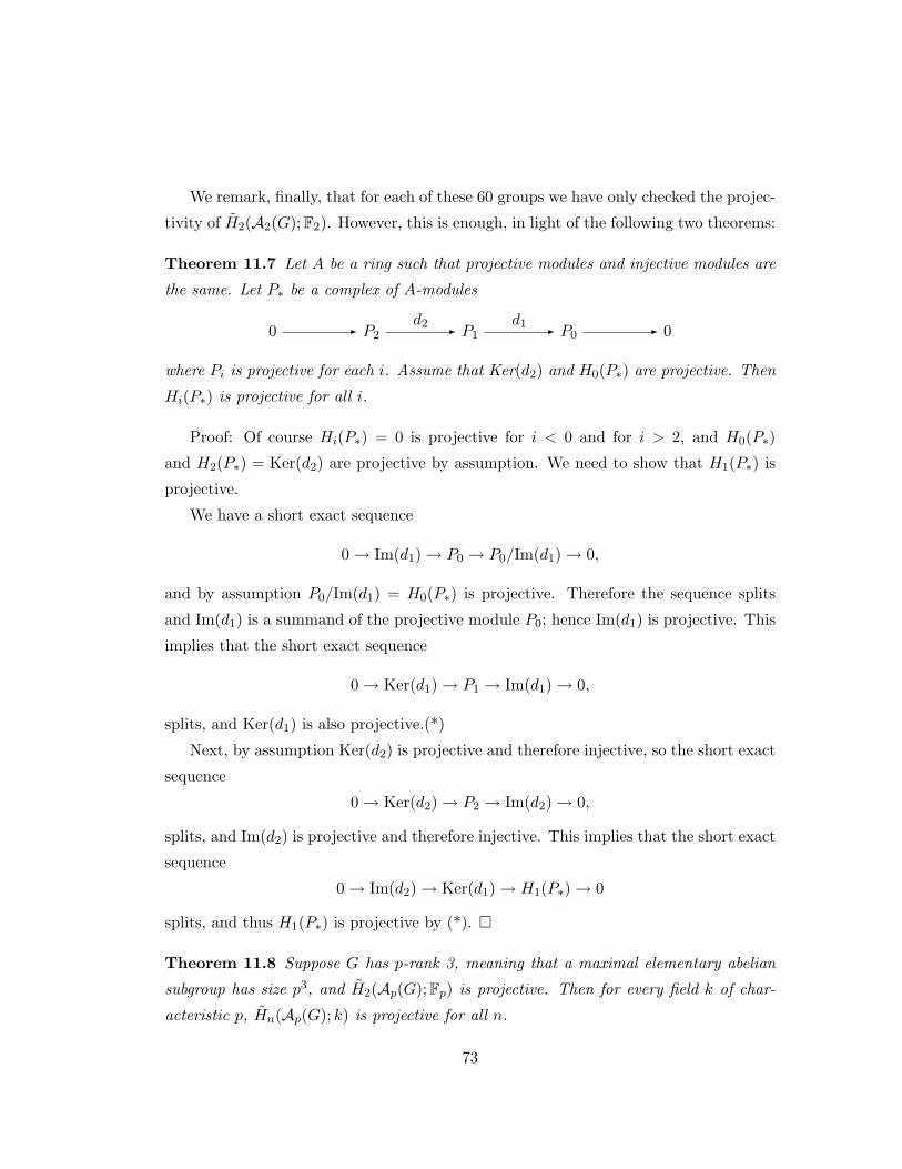
We remark, finally, that for each of these 60 groups we have only checked the projec-

tivity of H2(A2(G);F2). However, this is enough, in light of the following two theorems:

Theorem 11.7 Let A be a ring such that projective modules and injective modules are

the same. Let P∗ be a complex of A-modules

0 - P2d2 - P1

d1 - P0- 0

where Pi is projective for each i. Assume that Ker(d2) and H0(P∗) are projective. Then

Hi(P∗) is projective for all i.

Proof: Of course Hi(P∗) = 0 is projective for i < 0 and for i > 2, and H0(P∗)

and H2(P∗) = Ker(d2) are projective by assumption. We need to show that H1(P∗) is

projective.

We have a short exact sequence

0→ Im(d1)→ P0 → P0/Im(d1)→ 0,

and by assumption P0/Im(d1) = H0(P∗) is projective. Therefore the sequence splits

and Im(d1) is a summand of the projective module P0; hence Im(d1) is projective. This

implies that the short exact sequence

0→ Ker(d1)→ P1 → Im(d1)→ 0,

splits, and Ker(d1) is also projective.(*)

Next, by assumption Ker(d2) is projective and therefore injective, so the short exact

sequence

0→ Ker(d2)→ P2 → Im(d2)→ 0,

splits, and Im(d2) is projective and therefore injective. This implies that the short exact

sequence

0→ Im(d2)→ Ker(d1)→ H1(P∗)→ 0

splits, and thus H1(P∗) is projective by (*).

Theorem 11.8 Suppose G has p-rank 3, meaning that a maximal elementary abelian

subgroup has size p3, and H2(Ap(G);Fp) is projective. Then for every field k of char-

acteristic p, Hn(Ap(G); k) is projective for all n.

73

Proof:

By [55] we know that H0(Ap(G);Fp) is projective, so by Theorem 11.7, Hn(Ap(G);Fp)is projective for all n.

Let k be a field of characteristic p. By the Universal Coefficients Theorem,

H2(Ap(G); k) = k ⊗ H2(Ap(G);Z),

since the complex has dimension 2 and so the degree-2 integral homology is a free abelian

group and thus torsion-free. But then

k ⊗Z H2(Ap(G);Z) = (k ⊗Fp Fp)⊗ H2(Ap(G);Z)

= k ⊗Fp (Fp ⊗ H2(Ap(G);Z))

= k ⊗Fp H2(Ap(G);Fp).

So let P = H2(Ap(G);Fp), and let Q be such that P ⊕Q = FpGn. Then k⊗P ⊕k⊗Q =

k ⊗Fp (P ⊕Q) = k ⊗ FpGn = kGn. So k ⊗ P is projective.

So in this section we have proven the following:

Theorem 11.9 Suppose p and q are primes, and suppose J is a group of order paqb

for some positive integers a, b. If paqb < 25 ∗34, then the Steinberg complex of J , at any

prime r, over any r-complete local ring R, will have homology which in every dimension

is a projective RJ-module.

74

Chapter 12

A further look at coefficient

systems

We conclude by examining the properties of coefficient systems, and representations of

categories more generally. Recall that a representation of a category C over a ring R is

a functor from C to the category of R-modules. In section 3 we said that a coefficient

system is a contravariant functor, from the category of G-sets with stabilizers in a certain

collectionW of subgroups of G, to the category R-mod of finitely-generated R-modules.

Later on this section we will write O to mean the full subcategory of the category

of G-sets, whose objects are G-sets of the form G/H for some subgroup H. This is

the orbit category of G, and is equivalent to the category of all transitive G-sets. For

now, however, we will work in a more general setting, where we do not use special poset

categories W or O, but any small category C.Note: in the following discussion, where the word “functor” is used without descrip-

tor, it should be taken to mean “covariant functor.” When it comes time to consider

the special case of coefficient systems, we will be replacing C not by W or O, but by

Wop or Oop.

Definition 12.1 Let C be a small category, and R a commutative ring with identity.

If x is an object of C, then we write xF = RHomC(x,−), where for each object y of C,

RHomC(x, y) is defined to be the free R-module with basis the set of morphisms from x

75

to y in C. If f ∈ HomC(a, b), then we define xF (f) : xF (a)→ xF (b), or equivalently

xF (f) : RHomC(x, a)→ RHomC(x, b),

by giving its values on generators, according to the rule

(α : x→ a) 7→ (f α : x→ b).

Thus for each object x of C, we get a covariant functor xF : C → R-mod. How-

ever, a morphism h ∈ HomC(y, z) induces a natural transformation ηh : zF → yF , or

equivalently

ηh : RHomC(z,−)→ RHomC(y,−),

in the following way: at each object a of C, we have that ηah is given on generators by

(α : z → a) 7→ (α h : y → a).

So −F is a contravariant functor from C to the category (R-modC), which has for

its objects the functors C → R-mod and for its morphisms the natural transformations

between these functors.

Proposition 12.2 (Webb, Proposition 4.4 in [54]) Let C be a small category with

finitely many objects. Then:

(1) If M : C → R-mod is a functor, then HomRC(xF,M) ∼= M(x) as R-modules. (We

may think of representations of C over R as RC-modules; hence the notation HomRC.)

(2) xF is a projective RC-module.

Remark: The proofs go exactly as they did in section 3 for the special case of

coefficient systems. We rely on the assumption that C be a small category with finitely

many objects in order to identify (R-mod)C with RC-mod, where RC is the category

algebra: namely, the free R-module generated by the set of morphisms of C, with

multiplication defined on generators f and g by:

f ∗ g =

f g if f g is defined

0 else.

76

If it happens to be the case that C has one object and its morphisms form a group G

under composition, then RC is the group algebra RG, a functor C → R-mod is exactly

a representation of G over R, and the the equivalence is well-known. The equivalence

in the general case, along with many many other theorems of representation theory of

categories, is due to Webb and may be found in [54].

We note by way of example that the category algebra RC has identity element∑X∈Ob(C) IdX . Requiring C to have only finitely many objects ensures that this sum

will be finite.

Definition 12.3 For any functors M,N : C → R-mod, we define a functor (M ⊗N) :

C → R-mod by (M ⊗ N)(X) = M(x) ⊗R N(X) for any object X of C. If f : X → Y

is a morphism in C, then (M ⊗ N)(f) : (M ⊗ N)(X) → (M ⊗ N)(Y ) is defined as

M(f)⊗N(f) : M(X)⊗N(X)→M(Y )⊗N(Y ).

We also define Hom(M,N) : C → R-mod, by Hom(M,N)(y) := HomRC(yF ⊗M,N), for all objects y of C. Thus if y ∈ Ob(C) and F,M,N are functors C → R-

mod, then Hom(M,N)(y) is the set of natural transformations from yF ⊗ M to N .

This set of natural transformations is itself an R-module. Now if f : x → y is a

morphism in C, then f induces maps yF → xF , hence yF ⊗M → xF ⊗M , and finally

Hom(M,N)(x)→ Hom(M,N)(y).

We have defined Hom so that we have the following adjoint relation:

Proposition 12.4 Hom(L,Hom(M,N)) ∼= Hom(L⊗M,N) as R-modules.

Proof: Hom(zF ⊗M,N) = Hom(M,N)(z) = Hom(zF,Hom(M,N)), so the equa-

tion holds when L = zF , and more generally when L =⊕

ziF . For a general L we

take a projective resolution of L, or indeed a free resolution. We note that RC =⊕x∈Ob(C)RC ∗ Idx ∼=

⊕x∈Ob(C)

xF , so that a free resolution will be made of sums of

various xiF . Thus:

. . .→⊕

yjF →⊕

xiF → L→ 0

is exact, so

0→ Hom(L⊗M,N)→ Hom((⊕xiF )⊗M,N)→ Hom((⊕yjF )⊗M,N)

77

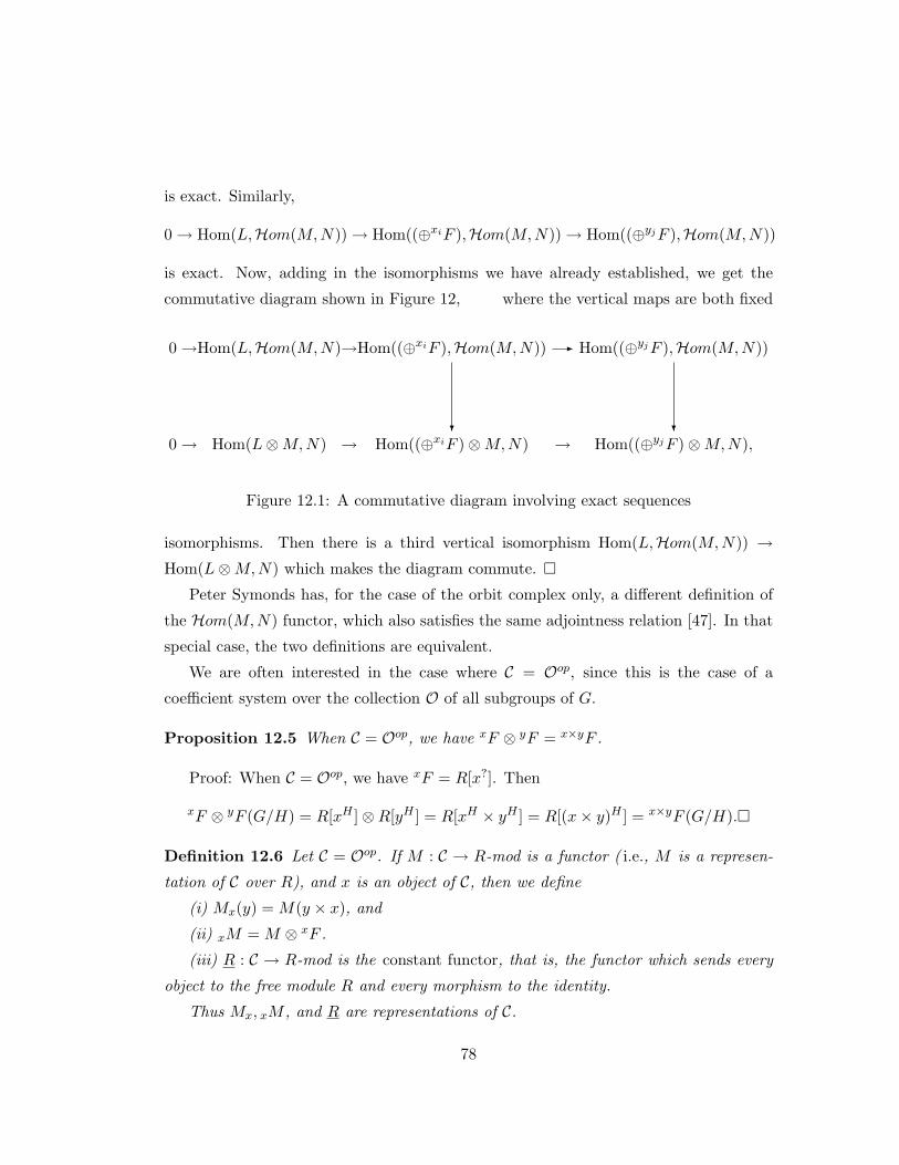
is exact. Similarly,

0→ Hom(L,Hom(M,N))→ Hom((⊕xiF ),Hom(M,N))→ Hom((⊕yjF ),Hom(M,N))

is exact. Now, adding in the isomorphisms we have already established, we get the

commutative diagram shown in Figure 12, where the vertical maps are both fixed

0→Hom(L,Hom(M,N)→Hom((⊕xiF ),Hom(M,N)) - Hom((⊕yjF ),Hom(M,N))

0→ Hom(L⊗M,N) → Hom((⊕xiF )⊗M,N)?

→ Hom((⊕yjF )⊗M,N),?

Figure 12.1: A commutative diagram involving exact sequences

isomorphisms. Then there is a third vertical isomorphism Hom(L,Hom(M,N)) →Hom(L⊗M,N) which makes the diagram commute.

Peter Symonds has, for the case of the orbit complex only, a different definition of

the Hom(M,N) functor, which also satisfies the same adjointness relation [47]. In that

special case, the two definitions are equivalent.

We are often interested in the case where C = Oop, since this is the case of a

coefficient system over the collection O of all subgroups of G.

Proposition 12.5 When C = Oop, we have xF ⊗ yF = x×yF .

Proof: When C = Oop, we have xF = R[x?]. Then

xF ⊗ yF (G/H) = R[xH ]⊗R[yH ] = R[xH × yH ] = R[(x× y)H ] = x×yF (G/H).

Definition 12.6 Let C = Oop. If M : C → R-mod is a functor ( i.e., M is a represen-

tation of C over R), and x is an object of C, then we define

(i) Mx(y) = M(y × x), and

(ii) xM = M ⊗ xF .

(iii) R : C → R-mod is the constant functor, that is, the functor which sends every

object to the free module R and every morphism to the identity.

Thus Mx, xM , and R are representations of C.

78

In particular, xR = xF , and MG/G = M = G/GM .

Now, given a map of G-sets x → z in O, hence z → x in C = Oop, we get natural

transformations Mz → Mx and xM → zM . Thus if ∆ is a G-simplicial chain complex,

we get complexes

M∆ = . . .→ 0→M∆−1 →M∆0 →M∆1 → . . .

and

∆M = . . .→ ∆1M → ∆0M → ∆−1M → 0→ . . . .

Proposition 12.7 Let C = Oop, and let M and N be representations of C over R.

Then:

1) (Mx)y = Mx×y.

2) y(xM) = y×xM

3) xM ⊗ yN = x×y(M ⊗N).

4) R∆ = Hom(∆R,R) = Hom(R[∆?], R).

5) Hom(yR,N) = Ny.

6) Hom(xM,N) = Hom(M,Nx).

7) Hom(M,Nx) = (Hom(M,N))x.

Proof:

1) (Mx)y(z) = M(z×x×y) = Mx×y(z). All the equalities are natural isomorphisms.

2) y(xM) = yF ⊗ (xF ⊗M) = (yF ⊗ xF )⊗M = y×xF ⊗M = y×xM .

3) xM⊗ yN = xF ⊗M⊗ yF ⊗N = xF ⊗xF ⊗M⊗N = x×y(M⊗N) = x×y(M⊗N).

4) By (3), taking N = R, we get Ry = Hom(yR,R). Thus

R∆ = Hom(∆R,R) = Hom(R[∆?], R).

5) Hom(M,N)(x) = Hom(xF ⊗M,N) for all M,N . Now taking M = yF = yR, we

get Hom(yF,N)(x) = Hom(x×yF,N). By the Yoneda lemma, this is Ny(x).

6) Hom(M,Nx) = Hom(M,Hom(xF,N)) ∼= Hom(M ⊗ xF,N) = Hom(xM,N).

7) Hom(M,N)x(y) = Hom(M,N)(x× y) = Hom(x×yF ⊗M,N) = Hom(yF ⊗ xF ⊗M,N) = Hom(xF ⊗M,N)(y) = Hom(xM,N)(y) = Hom(M,Nx)(y).

79

Theorem 12.8 (Eilenberg-Zilber, Theorem 3.1 in [28].) Let X and Y be topological

spaces. Then there exists a chain homotopy equivalence

ζ : C(X)⊗ C(Y )→ C(X × Y )

which is natural in X and Y – that is, given continuous maps f : X → X ′ and g : Y →Y ′, the diagram in Figure 12.8 commutes.

C(X)⊗ C(Y )ζ- C(X × Y )

C(X ′)⊗ C(Y ′)

f] ⊗ g]

? ζ- C(X ′ × Y ′)

(f × g)]

?

Figure 12.2: The Eilenberg-Zilber theorem for Coefficient Systems

We remark that the proof of this theorem does not require taking coefficients in the

ring Z; we can take C(−) to be C∗(−;R) for any commutative ring R, by applying the

functor −⊗R everywhere.

Theorem 12.9 Let G be a finite group, let R be a commutative ring with identity, and

let ∆,Θ be G-simplicial complexes. Then there exists a chain homotopy equivalence

R[(∆×Θ)?] ' R[∆?]⊗R[Θ?].

Thus these complexes are isomorphic in the homotopy category of coefficient systems.

Proof: For each H ≤ G, we have (∆ × Θ)H = ∆H × ΘH as simplicial complexes.

Thus R[(∆×Θ)H ] = R[∆H×ΘH ]. Therefore by the Eilenberg-Zilber Theorem, C∗(∆×Θ)H ;R) ' C∗(∆H ;R) ⊗ C∗(ΘH ;R). Rewriting to change notation, we get a chain

homotopy equivalence ζH : R[(∆×Θ)H ] ' R[∆H ]⊗R[ΘH ].

Finally, we need these equivalences to be natural in H, so that if H ≤ Kg, then the

following diagram commutes:

80

R[(∆×Θ)H ]ζH- R[∆H ]⊗R[ΘH ]

R[(∆×Θ)Kg]

6

ζKg

- R[∆Kg]⊗R[ΘKg

]

6

Fortunately, the inclusion and conjugation maps are continuous, so the naturality

condition is guaranteed by the Eilenberg-Zilber Theorem. Finally, we also require that

all the chain homotopies involved are natural in X and Y ; this is the content of Lemmas

5.7 and 5.8 in [28].

Remark: a chain map of complexes f : F∗ ' G∗ of coefficient systems is a doubly-

indexed family of R-module maps, fn(H) : Fn(H) → Gn(H). Fixing n and letting H

vary gives a morphism of coefficient systems Fn → Gn. Fixing H and letting n vary

gives a chain map of complexes of R-modules, F∗(H) → G∗(H). We have chosen to

define a chain map of complexes of coefficient systems using the second approach: for

each H the Eilenberg-Zilber Theorem guarantees the existence of a certain chain map

of complexes of R-modules, and also that the collection of all these maps is natural in

H.

Theorem 12.10 Let G be a finite group, let O be the set of all subgroups of G, and let

∆ = C∗(Sp(G);R). If Op(G) = 1 then EndROop(∆R) is chain homotopy-equivalent to

the complex which is R concentrated in degree 0. If Op(G) 6= 1 then EndROop(∆R) is

chain homotopy-equivalent to the zero complex.

Proof: We form the double complex with terms

Hom(⊕

σ∈G\∆i

R[(G/Gσ)?],⊕

τ∈G\∆j

R[(G/Gτ )?]) =⊕σ,τ

R[(G/GGστ )],

whose homology is homotopy classes of maps. We filter the double complex so that we

get a page of the spectral sequence made up of complexes R[∆Gσ ] for each σ. When

dim σ ≥ 0 this is contractible and gives 0 in homology. When dim σ = −1, we have

Gσ = G (every group element fixes the empty simplex). If another simplex is fixed

then it means that some nonidentity p-subgroup of G is normal in G, or in other words

81

Op(G) 6= 1. In that case ∆ 'G 0 and ∆R = 0. Hence at the next page, when Op(G) = 1,

there is only one non-zero term, in position (−1,−1), giving R.

It would be nice if in fact Hom(∆R,∆R) were R. If so, that would suggest the

possibility of a duality operator Hom(−,∆R) on complexes of coefficient systems, which

in particular interchanged ∆R and R.

Or it might signify a “tilting” property that the Steinberg complex in general did not

have. Recall that the Steinberg complex was found essentially by taking the complex

R[∆?] of coefficient systems, and evaluating in each dimension at the identity subgroup.

The resulting complex of RG-modules did not have a desirable tilting property in gen-

eral: the complex admitted nonzero self-chain maps in positive or negative degree. It

may be that it is more desirable not to evaluate at the identity subgroup, since we would

in essence then retain more conditions that a chain map has to satisfy, and thus allow

fewer chain maps to interfere with the tilting condition.

82

References

[1] J.L. Alperin, A Lie approach to finite groups. Groups–Canberra 1989, 1-9, Lecture

Notes in Mathematics 1456, Springer, Berlin, 1990.

[2] J.W. Ballard, Some generalized characters of finite Chevalley groups. Mathematis-

che Zeitschrift 147 (1976), 163-174.

[3] Michael Barr, Acyclic Models. Centre de Recherches Mathematiques 17, 2002.

[4] Glen E. Bredon, Equivariant Cohomology Theories. Lecture Notes in Mathematics

34, Springer-Verlag, 1967.

[5] Igor Burban and Yuriy Drozd, Derived categories of nodal al-

gebras. Journal of Algebra 272 (2004) 46-94. Available at:

http://www.imath.kiev.ua/~drozd/nodal.pdf

[6] Dave Benson, Representations and Cohomology, Vol II. Cambridge studies in ad-

vanced mathematics 31, 1991.

[7] Kenneth Brown, Euler characteristics of groups: The p-fractional part. Inventiones

Mathematicae 29 (1975), 1-5.

[8] Kenneth Brown, Cohomology of Groups. Graduate Texts in Mathematics 87,

Springer-Verlag, 1982.

[9] Serge Bouc, Resolutions de foncteurs de Mackey. Group representations: cohomol-

ogy, group actions and topology (Seattle, WA 1996), 31-83, Proc. Sympos. Pure

Math 63, Amer. Math. Soc., Providence, RI, 1998.

83

[10] M. Broue, Rickard Equivalences and Block Theory. Groups ’93, Galway/St Andrews

Vol 1, 58-79, London Mathematical Lecture Note Series 211, Cambridge University

Press, 1995.

[11] Marc Cabanes and Jeremy Rickard, Alvis-Curtis duality as an equivalence of de-

rived categories. Modular representation theory of finite groups (Charlottesville,

VA, 1998), 157-174, de Gruyter, Berlin, 2001.

[12] Roger W. Carter, Finite Groups of Lie Type: Conjugacy Classes and Complex

Characters. John Wiley and Sons, 1985.

[13] P.M. Cohn, Further Algebra and Applications. Springer, 2003.

[14] Charles W. Curtis and Irving Reiner, Methods of Representation Theory, Vol. II.

John Wiley and Sons, 1987.

[15] Francois Digne and Jean Michel, Representations of Finite Groups of Lie Type.

London Mathematical Society Student Texts 21, 1991.

[16] William G. Dwyer, Sharp homology decompositions for classifying spaces of finite

groups. Group representations: cohomology, group actions and topology (Seattle,

WA, 1996), 197-220, Amer. Math. Soc., Providence, RI, 1998.

[17] William G. Dwyer and Hans-Werner Henn, Homotopy Theoretic Methods in Group

Cohomology. Advanced Courses in Mathematics. CRM Barcelona. Birkhauser Ver-

lag, Basel 2001.

[18] Walter Feit, Extending Steinberg characters. Linear Algebraic Groups and Their

Representations (Los Angeles, CA, 1992), 1-9, Contemporary Mathematics 153,

American Mathematical Society, 1993.

[19] George Glauberman, On Burnside’s other paqb theorem, Pacific J. Math. Vo. 56

No. 2 (1975), 469-476.

[20] Daniel Gorenstein, Finite Groups. Harper and Row, 1968.

[21] J. Grodal, Higher limits via subgroup complexes, Annals of Mathematics 155

(2002), 405-457.

84

[22] G.D. James, The Representation Theory of the Symmetric Groups, Lecture Notes

in Mathematics 682, Springer-Verlag, 1978.

[23] Stefan Jackowski, James McClure and Bob Oliver, Homotopy classification of self-

maps of BG via G-actions I and II, Annals of Mathematics 135 (1992), 183-226;

227-270.

[24] Stefan Jackowski, James McClure and Bob Oliver, Homotopy theory of classify-

ing spaces of compact Lie groups. Algebraic topology and its applications, 81-123,

Springer, New York, 1994.

[25] Chao Ku, A new proof of the Solomon-Tits Theorem, Proceedings of the American

Mathematical Society Vol 126, Number 7 (July 1998), 1941-1944.

[26] George Lusztig, Divisibility of projective modules of finite Chevalley groups by

the Steinberg character, Bulletin of the London Mathematical Society 8 (1976),

130-134.

[27] Markus Linckelmann and Sibylle Schroll, On the Coxeter complex and Alvis-Curtis

duality for principal `-blocks of GLn(q), Journal of Algebra and Applications 4

(2005), 225-229.

[28] Massey, William S. A Basic Course in Algebraic Topology, Graduate Texts in Math-

ematics 121, Springer-Verlag, New York, 1991.

[29] B. Mitchell, The Full Imbedding Theorem, American Journal of Mathematics 86

(1964), 619-637.

[30] B. Mitchell, Rings with several objects, Advances in Mathematics 8 (1972), 1-161.

[31] Bob Oliver, Higher limits via Steinberg Representations, Commutative Algebra 22

(1994), 1381-1393.

[32] Bodo Pareigis and Helmut Rohrl, Complements and the Krull-Schmidt Theorem

in arbitrary categories, Applied categorical structures 3 (1995), 11-27. Available at:

http://www.springerlink.com/content/n759116773361336/fulltext.pdf

85

[33] Daniel Quillen, Homotopy Properties of the Poset of Nontrivial p-Subgroups of a

Group, Advances in Mathematics 28 (1978), 101-128.

[34] Robinson, Derek J.S., A Course in the Theory of Groups, Second Edition. Graduate

Texts in Mathematics 80, Springer-Verlag, 1996.

[35] A. J. E. Ryba, Stephen D. Smith and Satoshi Yoshiara, Some projective modules

determined by sporadic geometries, Journal of Algebra 129 (1990), 279-311.

[36] Shokuev, V.N., Generalizations of Hall’s principle of enumeration, Matem. Zapiski

6, No. 1 (1967), 124-143.

[37] Shokuev, V.N., The enumeration of subgroups in finite p-groups, Matem-

aticheskie Zametki, Vol. 13, No. 1, (1967), 107-112. English translation:

Springer Mathematical Notes, Vol. 13, No. 1 (January 1973). Available at

http://www.springerlink.com/content/t83761508282u874/fulltext.pdf

[38] Louis Solomon, The Steinberg character of a finite group with a BN -pair. Theory

of Finite Groups (Symposium, Harvard Univ., Cambridge, MA, 1968), 213-221,

Benjamin, New York, 1969.

[39] Robert Steinberg, Prime power representations of finite linear groups I, II, Cana-

dian Journal of Math 8 (1956), 580-591; 9 (1957), 274-282.

[40] Yoav Segev and Peter Webb, Extensions of G-posets and Quillen’s Complex, J.

Austral. Math. Soc. (Series A) 57 (1994), 60-75.

[41] Dan Swenson, Answers to some questions posed

to me by my adviser, Peter Webb. Available at:

http://www.math.umn.edu/~dswenson/Research/newsteinbergcomplex.pdf

[42] Dan Swenson, Untitled. Available at: http://www.math.umn.edu/~dswenson/Research/wreath.pdf.

[43] Dan Swenson, The Steinberg complex. Available at:

http://www.math.umn.edu/~dswenson/Research/oralprelim.pdf.

[44] Dan Swenson, A different wreath product. Available at:

http://www.math.umn.edu/~dswenson/Research/newwreath.pdf.

86

[45] Peter Symonds, A Relative Version of a Theorem of Webb. Preprint, available at:

http://www.maths.manchester.ac.uk/~pas/preprints/equi.pdf

[46] Symonds, Peter, The orbit space of the p-subgroups complex is contractible, Com-

ment. Math. Helv. 73 (1998), 400-405.

[47] Peter Symonds, The Bredon Cohomology of Subgroup Complexes, Journal of Pure

and Applied Algebra 199 (2005), 261-298.

[48] Jacques Thevenaz, Permutation representations arising from simplicial complexes,

Journal of Combinatorial Theory. Series A 46 (1987), 121-155.

[49] Jacques Thevenaz and Peter Webb, Homotopy equivalence of posets with a group

action, Journal of Combinatorial Theory. Series A 56 (1991), 173-181.

[50] Jacques Tits, Theoreme de Bruhat et sous-groupes paraboliques, C. R. Acad Sci.

Paris, 254 (1962), 2910-2912.

[51] P.J. Webb, Subgroup Complexes. The Arcata Conference on Representations of

Finite Groups (Arcata, Calif., 1986), Proc. Sympos. Pure Math. 47, 349-365, A.

M. S., Providence, RI, 1987.

[52] P.J. Webb, A local method in group cohomology. Commentarii Math. Helv. 62

(1987), 135-167.

[53] P. J. Webb, A Split Exact Sequence of Mackey Functors, Comment. Math. Helv.

66 (1991), 34-69.

[54] P. J. Webb, An introduction to the representations and cohomology of categories.

Group Representation Theory, eds. M. Geck, D. Testerman and J. Thevenaz, EPFL

Press (2007), 34-69.

[55] P.J. Webb, Finite Group Representations for the Pure Mathematician. Available

at http://www.math.umn.edu/~webb/RepBook/.

[56] P.J. Webb, GAP teaching materials and routines written by Peter Webb. Available

at http://www.math.umn.edu/~webb/GAPfiles/.

87

[57] Charles A. Weibel. An Introduction to Homological Algebra, Cambridge studies in

advanced mathematics 38, 1994.

[58] Fei Xu, Homological properties of category algebras, Ph.D. thesis, University of

Minnesota 2006.

88

Appendix A

GAP routines used in calculations

It has been necessary to use computers to assist in some of the calculations performed

in this work. This has been done in GAP. The new software written for the purpose of

this work, specifically section 11, is presented here.

psubs:=function(g,p)

## This program calculates the different subgroup complexes for a group## g at a prime p.

local reps,sp,ap,bp,zp,i,elts,x;reps:=ConjugacyClassesSubgroups(g);reps:=List(reps,Representative);

sp:=[];for i in reps doif Size(i) in DivisorsInt(Size(SylowSubgroup(g,p))) thenif Size(i) > 1 thenAdd(sp,i);fi;fi;od;

ap:=[];for i in sp doif IsElementaryAbelian(i) thenAdd(ap,i);fi;od;

zp:=[];

89

for i in ap doelts:=[];for x in Center(Centralizer(g,i)) doif Order(x) in [1,p] thenAdd(elts,x);fi;od;if Group(elts) = i thenAdd(zp,i);fi;od;

bp:=[];for i in sp doif PCore(Normalizer(g,i),p) = i thenAdd(bp,i);fi;od;

return([sp,ap,zp,bp]);end;

#### Must read "reps" and "psubgroups" first.#### More importantly, this function as written only works for## p=2, and only for groups of 2-rank 3 (a maximal elementary abelian## 2-subgroup has order 2^3).#### This program checks whether or not the homology in dimension 2## of the Steinberg complex of a group g at the prime 2 over the## field of 2 elements is projective##

isproj2homology:=function(g)local z2,triangles,i,j,ori,orj,l,m,n,k,ork,lines,delta,null,

mats,mat,x,rep,count;if not 2 in DivisorsInt(Size(g)) then

return true;fi;z2:=psubs(g,2)[3];triangles:=[];;lines:=[];;for i in z2 do

90

for j in z2 doif Size(j) > Size(i) thenori:=ConjugateSubgroups(g,i);orj:=ConjugateSubgroups(g,j);for l in ori do

for m in orj doif IsSubgroup(m,l) then

Add(lines,[l,m]);fi;

od;od;for k in z2 do

if Size(k) > Size(j) thenork:=ConjugateSubgroups(g,k);for l in ori do

for m in orj dofor n in ork do

if IsSubgroup(m,l) and IsSubgroup(n,m) thenAdd(triangles,[l,m,n]);

fi;od;

od;od;

fi;od;

fi;od;

od;delta:=NullMat(Size(triangles),Size(lines),GF(2));for i in [1..Size(triangles)] doj:=1;count:=0;while count < 3 doif IsSubset(triangles[i],lines[j]) then

delta[i][j]:=Z(2)^0;count:=count+1;

fi;j:=j+1;

od;od;null:=NullspaceMat(delta);;

91

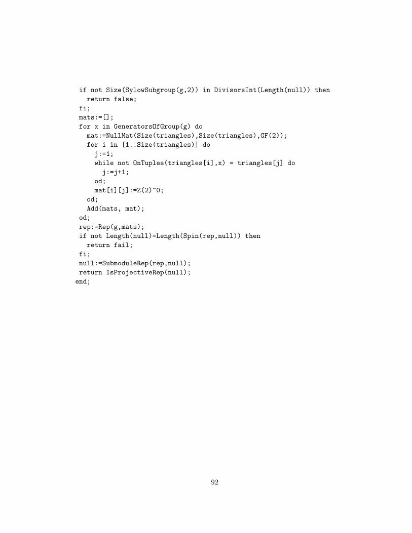
if not Size(SylowSubgroup(g,2)) in DivisorsInt(Length(null)) thenreturn false;

fi;mats:=[];for x in GeneratorsOfGroup(g) do

mat:=NullMat(Size(triangles),Size(triangles),GF(2));for i in [1..Size(triangles)] doj:=1;while not OnTuples(triangles[i],x) = triangles[j] do

j:=j+1;od;mat[i][j]:=Z(2)^0;

od;Add(mats, mat);

od;rep:=Rep(g,mats);if not Length(null)=Length(Spin(rep,null)) then

return fail;fi;null:=SubmoduleRep(rep,null);return IsProjectiveRep(null);end;

92