THE STEEPEST DESCENT GRAVITATIONAL METHOD FOR LINEAR PROGRAMMING

Discrete Applied Mathematics 25 (1989) 211-239 North-Holland

211

THE STEEPEST DESCENT GRAVITATIONAL METHOD

FOR LINEAR PROGRAMMING

Soo Y. CHANG* Department of Mathematical Sciences, Clemson University, Clemson, SC 29634-1907, USA

Katta G. MURTY* Department of Industrial and Operations Engineering, The University of Michigan, Ann Arbor, MI 48109-2117, USA

Received 22 December 1987

Revised 24 May 1988

We present a version of the gravitational method for linear programming, based on steepest descent gravitational directions. Finding the direction involves a special small “nearest point problem” that we solve using an efficient geometric approach. The method requires no expensive

initialization, and operates only with a small subset of locally active constraints at each step. Redundant constraints are automatically excluded in the main computation. Computational

results are provided.

Keywords. Gravitational method, steepest descent direction, feasible directions, redundant constraints, nearest point problem, simplicial cone.

1. Introduction

A new approach for solving linear programming problems (LP) called “the gravitational method” was introduced in the recent paper [25]. The method needs an initial interior feasible solution, from which the method traces a piecewise-linear descent path which is completely contained in the interior of the feasible region. For this reason, the method is an interior method. In each stage of the method, only a small locally defined set of constraints (these are the “touching” constraints or “active” constraints according to a special definition pertinent to this method) plays a role in the major computation, hence the method can be viewed as an active set method. The method can also be seen as a variant of the gradient projection method [28,29], since the directions taken by the method are in the form of the projection of the negative gradient on a face of the feasible region. However, it is very different from the usual gradient projection method both in the directions chosen, and in its philosophical foundations. Each step in the method finds a descent feasible direction and moves in that direction. These are the basic building blocks of methods of feasible directions pioneered by Zoutendijk [41-431, for this reason, the gravitational method can be viewed as a special case of methods of feasible directions.

* Partially supported by NSF Grant ECS-8521183, and NATO Grant RG 85-0240.

0166-218X/89/$3.50 0 1989, Elsevier Science Publishers B.V. (North-Holland)

212 S. Y. Chang, K.G. Murty

The gravitational method involves one or more stages. Each stage consists of an alternating sequence of direction finding and step length routines. The direction finding routine finds the direction to move by solving a small locally defined quadratic programming problem in the form known as “the nearestpointproblem” 1231. The major part of the computational effort of the algorithm goes into this routine. The step length routine performs a straight move in the selected direction, to the maximum extent possible, until a face of the feasible region blocks the movement in that direction.

For large scale practical problem solving, the gravitational method has several major advantages over other methods for linear programming. These advantages are:

(1) Karmarkar’s method, as it appeared in [16], needs an expensive initialization effort to transform the linear program into Karmarkar’s canonical form. The gravitational method needs no such expensive initialization.

(2) All the other interior point methods (Karmarkar’s method, method of centers, homotopy methods, etc. [l-3,5,10,12,13,15-17,19,20,27-32,36,39]) and all the variants of the simplex method, operate on all the constraints in every step. In the gravitational method however, only a small subset of constraints (called the “touching constraints”) comes into the major computation in each step of the method, and therefore the computational effort in each iteration is significantly less than that of other methods.

(3) Practical linear programming models usually contain quite a few redundant constraints. In the gravitational method, redundant constraints never enter into the major computation i.e. in the direction finding routine.

(4) The assumption of primal or dual nondegeneracy plays an important role in establishing finite convergence of the simplex method [7,24]. No such nondegeneracy assumption is required for the finite convergence proof of the gravitational method.

(5) All the other interior point methods generate only a “near optimum” interior feasible solution at termination. All of these methods depend on a final procedure, which is based on a pivotal method, to convert this near optimum solution into a true optimum solution. This final procedure may need a significant number of pivot steps (up to as many as the number of variables in the problem), hence it could become computationally expensive. The versions MGMl and MGM2 of the gravitational method discussed in Section 9 do not need any expensive final procedure like this, since they terminate with the actual primal optimum solution, if one exists. However, if the dual optimum solution is also wanted, some additional computation may be required.

In this paper, we present the steepest descent variant of the gravitational method, called SDGM in Section 6, and its finite convergence proof. However, in order to get an efficient practical computer implementation we modify this original method,

Gravitationai method for LP 213

and develop two variants called MGMl and MGM2 (Section 9), both of which also have the finite convergence property.

We provide the summary of a computational experiment comparing the performance of the gravitational method and the well-known simplex method under the computer implementation “MINOS version 5.0” [21]. This computer experiment reveals some promising results which will require much further testing.

2. Overview of the method

We consider an LP in the form,

maximize r&,

subject to nA = c, ~20 (1)

where A is a matrix of order m x n, z E lRm is the row vector of primal variables, t, E lRm is a column vector, and c E IR” is a row vector.

The dual problem of (1) is

minimize z(x) = CX,

subject to Axhb, (2)

where A, b and c are same as in (l), and XE IR” is the column vector of dual variables.

An LP in the form (1) is said to be in “standard form.” Before applying the simplex method, an LP is usually transformed into standard form by well-known simple transformations [7,22,24]. To solve an LP by the gravitational method, we first transform the LP into standard form, and then apply the gravitational method on the dual of the problem, which will be in the form (2). When the gravitational method is applied on (2), it will produce an actual optimum solution of (1) in a finite number of steps, if one exists. However, in some cases, additional computation is required to obtain a dual optimum solution (i.e. an optimum solution for (2)), when one exists.

To apply the gravitational method on the LP (2), we assume that a strict interior point of the feasible region (i.e. a point x0 satisfying Ax’> b) is available initially. If an interior point is not available, we transform the LP (2) by introducing an artificial variable xn+ , and modify the problem as follows

minimize cx+Mx,+t, (3)

subject to Ax+e~,+~~b, x,+~~O,

where e=(l, . . . . l)T E Rm and M is a positive number which is significantly larger than any other number in the problem. Many existing interior methods use this type of augmentation, and this is equivalent to the usual big-M augmentation with one


artificial variable as explained in the literature on the simplex method [7,22,24]. Letx~,.,>max{O,Bi:i=l ,..., m).Then, (0 ,..., 0,x:+ t) is a strict interior feasible

solution of (3). Thus the modified problem (3) has a known interior feasible solution, and is in the same form as (2).

So, we will assume that an initial interior feasible solution x0 for (2) is always available. We also assume that c#O, as otherwise every feasible solution to (2) is an optimum solution, and the initial interior feasible solution can itself be taken as an optimum solution, and rr = 0 is an optimum solution for (1).

The overall scheme of the gravitational method applied on (2) is explained by the following. Let K be the feasible region of (2). We introduce a heavy spherical liquid drop centered at x0 with radius E, which is chosen positive and small so that the entire drop is completely contained inside the feasible region. Make the faces of K im- permeable “walls” separating the inside of K from the outside. Then, introduce a powerful gravitational force in K in the direction -cT, which is the negative gradient of the objective function in (2), and release the drop. The drop will fall under the influence of the gravitational force. During its fall, the drop may touch the boundary of K, but the center of the drop will always be at a distance ge from the nearest point to it on the boundary.

First, the drop will move through the interior of K in the direction of the gravitational force -cT until it is blocked by a face of K that we call the “blocking face.” The falling drop will exert a pushing force in the gravitational direction, -cT, on the blocking face, which will result in a reaction force from the blocking face. After this action and reaction, the drop will roll down on the face itself until it is blocked by another face.

At some point in its fall, the drop may be touching one or more facets of K, which are called “touching facets,” and the constraints in (2) that define these facets are called “touching constraints” at the center of the drop. Being pulled down by the gravitational force, the drop will push these facets, and the facets will react. Then, wherever the balanced force leads the drop, the drop will move. If, however, the reaction forces of the touching facets completely cancel out the gravitational force, the drop will halt. This final halting position is the lowest possible point in the direction -cT, that the drop can get to in K. If the radius of the drop, E, is sufficiently small, the touching constraints of (2) at this final halting position, will determine an actual optimum solution of the LP (1).

In Fig. 1, we illustrate the path of the drop in its gravitational fall in a three- dimensional problem with an optimum solution. The method traces the path taken by the center of the drop as it falls freely under the influence of the gravitational force. We denote this path by Y.

The gravitational method consists of a sequence of steps where, each step consists of the following two substeps.

Substep 1. Find the gravitational direction at the current interior feasible solution. This is defined to be the direction in which the drop will move next when it is in

Gravitational method for LP 215

initialcenterofthe drop

optimum point

Fig. 1. Illustration of the path of the drop in its fall under the influence of the gravitational force.

position with its center at the current point. There are two possible outcomes in this substep.

(i) It may be determined that the drop cannot move any further, in this case the drop halts.

(ii) The gravitational direction at the current center may be obtained, then go to Substep 2.

Substep 2. Move as far as possible in the gravitational direction determined in Substep 1. In this substep, we move the drop straight in the gravitational direction to the maximum extent possible, until it is blocked again by the boundary of the feasible region. The step length of the move is determined by the usual minimum ratio test.

If this step length is finite, update the center and go to the next step. If the step length is infinite, the objective function is unbounded below on the set of feasible solutions of (2). In this case, (1) is infeasible.

A stage in the gravitational method begins with the release of the drop and ends either when the drop halts or, when the step length in some step turns out to be 03. If the drop halts, from the equations of force balance, we can get a feasible solution for (1), and thus a lower bound on the optimum objective value in (2). A final special step is carried out at that time. This final special step involves projection on the affine space determined by the touching constraints at that time, treated as equations. If this final step yields a feasible solution for (2), we have the primal and dual optimum solutions for (1). Otherwise, we perform the radius reduction process in which we define a new drop with a reduced radius to initiate the next stage. The gravitational method yields an actual optimum solution for (I), after at most finite number of stages.

3. Notation

For ease of reading this paper, we summarize the notation here.

IFI cardinality of a set F,

\ set difference symbol, e.g. F, \ Fz = (i: i in F,, but not in Fz},

216

II4 K

Ai.

AJ.

4X: ~1

x0

x’

Jf-9

GW

Yr

JB(Y’)

Y

tl

D

4

RPosv-)

BFS SDGM

S. Y. Chang, K.G. Murty

Euclidean norm of a vector v; the feasible region of (2), {x: Axzb}; ith row of A; a matrix consisting of rows Ai. for iE J, spherical liquid drop centered at the point xr with radius E; initial interior point of K;

center of the drop after r steps; index set of touching constraints for the drop B(E,c), this is {i: Ai.Z=bi+& [[A,.[/); set of descent feasible directions for the drop B@, c), this is ( y: cy< 0, and Ai.ygO for all icz J(f)}; gravitational direction at x’, this is the steepest descent direction among those in G(x’); index set of blocking constraints in the direction yr$ this is {i: Ai.y’<O); piecewise linear path of the center of the drop in its gravitational descent in a stage, that is the piecewise linear path connecting x0,x’, . . . ; row vector of variables in the nearest point problem corresponding to the gravitational direction finding subroutine in a step; dimension of 4 changes from step to step, it is always equal to the cardinality of the touching constraints index set in that step; the matrix consisting of rows Ai. for i in the index set of touching constraints in a step; there is a variable in q for each row of D; the residual vector in a step, e is a row vector in mn; c =c-qD with the optimum 11 in that step; if LJ#O, the gravitational direction in that step is -<T/II~II.

defined when F is either a matrix, or a set of row vectors in II?“; it is the cone which is the nonnegative hull of row vectors in 10; basic feasible solution; steepest descent gravitational method, that is, the one based on the direction finding routine discussed in Section 6.

4. Initialization

To initiate the first stage of the method, select E to satisfy,

O<a<min Ai.XO- bi

IIAi. II : i= l,...,m

1 . (4)

Since the Euclidean distance of x0 from the hyperplane {x: Ai. x = bi} is Ai.x’- bi/I[Ai. 11, the liquid drop B(x’, e) does not intersect any of the hyperplanes {X: Ai.X=bi} for all i= l,..., m.


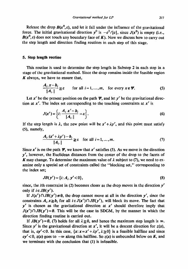
Release the drop B(x”,c), and let it fall under the influence of the gravitational force. The initial gravitational direction y” is -cT/llcll, since J(x’) is empty (i.e., B(x”, 8) does not touch any boundary face of K). Now we discuss how to carry out the step length and direction finding routines in each step of this stage.

5. Step length routine

This routine is used to determine the step length in Substep 2 in each step in a stage of the gravitational method. Since the drop remains inside the feasible region K always, we have to ensure that,

Ai.X- bi

/Ai. 11 ” for all i= I,..., m, for every XE P.

Let xr be the present position on the path !P, and let yr be the gravitational direction at xr. The index set corresponding to the touching constraints at x’ is

Ai.X’-bi IIAi. II (6)

If the step length is Iz, the new point will be xr+ly’, and this point must satisfy (3, namely,

(7)

Since x’ is on the path Y, we know that x’ satisfies (5). As we move in the direction y’, however, the Euclidean distances from the center of the drop to the facets of K may change. To determine the maximum value of Iz subject to (7), we need to ex- amine only a special set of constraints called the “blocking set,” corresponding to the index set;

JB(y’)=(i: Ai.y’<O}, (8)

since, the ith constraint in (2) becomes closer as the drop moves in the direction yr only if iED(

If J(x’) fl JB(y’)+O, the drop cannot move at all in the direction yr, since the constraints Ai.xg bi for all ie J(x’) n JB(y’), will block its move. The fact that yr is chosen as the gravitational direction at xr should therefore imply that J(x’) fl JB(y’) =0. This will be the case in SDGM, by the manner in which the direction finding routine is carried out.

If JB(y’) =0, (7) holds for all 120, and hence the maximum step length is 00. Since yr is the gravitational direction at x’, it will be a descent direction for E(X), that is, cy’ CO. In this case, {x: x=xr + Ay’, 1201 is a feasible halfline and since cy’<O, z(x) goes to -OO along this halfline. So z(x) is unbounded below on K, and we terminate with the conclusion that (1) is infeasible.


If JB(y’)#O, the maximum step length is

e=Min Ai.x’-4-c IIAi.11 : iEJBtyrJ -Ai.Y’ 1

. (9)

So, the step length in this case is 8, this moves the center of the drop to the next point x’+ ’ - --x’+6y’, with which the method proceeds to the next step.

6. Gravitational direction finding routine in SDGM

Suppose the drop is in position with its center at 5. So, f must satisfy (5). The version presented in this section seeks the steepest descent direction among all the directions that the drop can move from the present position. Hence, the version of the gravitational method discussed in this section will be called the steepest descent gravitational method, or SDGM. We show that the problem of finding the steepest descent gravitational direction is a special case of a well-known quadratic programming problem called the “nearest point problem. ”

We define the set of descent feasible directions at Z, denoted by G(X), to be the directions y satisfying,

CY<O, Ai.Q+Ay)-bi ,E

IPi. II = for all i= 1, . . . . m, and for some L > 0.

The set G(X) consists of all directions along which the drop can move a positive length in gravitational descent, while still remaining inside K, when its center is in position at R. Clearly, G(Z) = { y: cyC0, and Ai. YZO for all ie J(2)).

J(Z) = 0 if and only if the entire drop B@, e) is strictly in the interior of K without intersecting the boundary of K. In this case, G(Z) = { y: cyc 0). The gravitational direction in this case is the direction of the gravitational force itself (since the drop can move in all directions in this case), namely -cT/llcll.

Now, suppose J(X) #0. In this case, the gravitational direction at f is a direction selected from G(X) along which the drop can move from its current position. There are many different principles which can be used for making this selection. One principle discussed in [25] based on gradient projection, may take several steps before making the selection. In the version presented in this paper, we define the gravitational direction as the steepest descent direction among all the descent feasible directions at f, that is, those in G(X). Hence, it is the optimum solution of the following problem:

minimize cy,

subject to AJcj,. yz 0, 1 - yryzo. (11)


Remark 6.1. Problem (11) is in the same form as the problem for determining the direction of movement in Zoutendijk’s methods of feasible directions [41-431, par- ticularly that labelled “AZ1 with L.z norm criterion.” We would like to point out the differences. Our direction finding problem (11) comes from our physical model of the falling drop, here E is the radius of this drop, it has to satisfy (4), and it is the Euclidean distance of the present interior feasible solution R to each of the touching facets. In Zoutendijk’s method with AZl, e is a positive parameter used for anti-zigzagging precaution. These two problems can lead to completely different answers. As an example, consider the linear program,

minimize x1 + 2x2,

subject to 32x, 20, 8x2 2 0.

Let z=(l, l)T and e= 1. For this example, Zoutendijk’s AZ1 with L2 norm criterion leads to the direction finding problem

minimize Yl +a29

subject to 1 -YTYsO,

which has the solution ( - l/6, -2/e). For the same example, our problem (11) is

minimize YI +2y2,

subject to 32yi ~0,

which has the solution (40).

8~2 B 0, 1 -yTyzO,

Besides, the manner in which we use the direction finding problem (11) is very different from that in Zoutendijk’s method with AZl. Later on we develop im- plementations (MGMl and MGM2) in which only a subset of the linear constraints in (1 l), those corresponding to a linearly independent subset of row vectors, is used. Furthermore, we use an efficient geometric approach for solving the direction finding problem, which is entirely different from Zoutendijk’s approach.

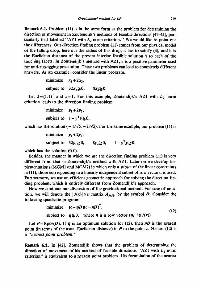
Now we continue our discussion of the gravitational method. For ease of notation, we will denote the /J@)/ xn matrix AJcs,. by the symbol D. Consider the following quadratic program:

minimize (c-tlD)(c-rtl))T, (12)

subject to ~20, where q is a row vector (qi: i E J(X)).

Let P=Rpos(D). If 1 is an optimum solution for (12), then flD is the nearest point (in terms of the usual Euclidean distance) in P to the point c. Hence, (12) is a 4 ‘nearest point problem. ”

Remark 6.2. In [43], Zoutendijk shows that the problem of determining the direction of movement in’his method of feasible directions “AZ1 with L2 norm criterion” is equivalent to a nearest point problem. His formulation of the nearest

220 S. Y. Chang, K. G. Murty

point problem is different from (12) in two ways. First, as pointed out in Remark 6.1, the system of linear inequality constraints in his direction finding problem can be quite different from those in (11) under the gravitational method. Second, even if these constraints are tbe same, Zoutendijk’s nearest point problem is the following:

minimize c-c-YTE-CT-Y),

subject to 0~20,

which is different from (12). Zoutendijk’s is the problem of finding a nearest point in a cone defined by linear inequalities. On the other hand, (12) is the problem of finding the nearest point in a cone which is expressed as the nonnegative hull of the touching constraints row vectors. The form in which (12) is expressed, makes it possible for us to use efficient special geometric procedures discussed in [23,26,33-351 to solve it.

See Fig. 2 for an example. In this example, the coefficient vectors corresponding to the active constraints are called {A, .,AZ.}. The nearest point of Zoutendijk’s method is p’ in Fig. 2(a), and the nearest point in the gravitational method is p2 in Fig. 2(b).

Zoutendijk 1431 proved the equivalence of his direction finding problem to the nearest point problem considered by him, by showing that the optimality conditions for the two problems are the same. In the following lemma, we will prove the equivalence of (11) and (12) using exactly the same technique.

Lemma 6.3. For each q 2 0, define 4 = c - qD. Let ij be the optimum solution for (12), and let c=c- ijD. Define jj by

-_ -~T415119 if009 y- 0 t , if <=O.

Then, Jo is the optimum solution for (11).

Proof. Both (11) and (12) have optimum solutions. Both are convex programming

Fig.2. The nearest points in Zoutendijk’s method and the gravitational method.


problems, and hence the first-order necessary optimality conditions are both necessary and sufficient for optimality in them.

Let o = (oi: i~J(z)), BE IR be the Lagrange multipliers corresponding to the constraints in (11). Remembering that D=A,,,. , the first-order optimality conditions for (11) are,

c-oD+26yT=0, (13a)

DYSO, 1 - y*yzo, (13b)

020, 620, (13c)

0Dy = 0, 6(1 -yTy)=O. (13d)

Let p = (pi: i E J(Z)), be the Lagrange multipliers corresponding to the constraints in (12). The first-order optimality conditions for (12) are,

- 2cDT + 2qDD* -F = 0, (W

rlL0, PLO, W)

C(q* = 0. (W

Since ij is an optimum solution of (12), there must exist a vector p such that (&/i) satisfy (14). Define

@=ij, 6=+lic-fjDII (15)

and verify that (a, &jr) satisfy (13). Hence, the lemma follows. Cl

Hence, if e#O, the gravitational direction at z is - <*/Ilell. If however c=O, we will now prove that G(Z), the set of descent feasible directions at 2, is empty.

Theorem 6.4. Let t=c - fjD where 1 is an optimum solution of (12). If r=O, G(z) = 0.

Proof. By hypothesis, 0 is a feasible solution for the system.

qD=c, t/20.

Then, by Farkas’ lemma, the following system is infeasible.

CY<O, DY~O,

which is the system that defines G(Z). 0

Let fl be an optimum solution for (12). q is called an optimum q-vector for this step. c= c - tiD is called the residual vector in this step.

If r= c - fjD = 0, by Theorem 6.4, G(Z) = 0, this implies that the drop B(Z, E) cannot move any further in gravitational descent, and hence it halts. The equation


c - QD = 0 also shows that the gravitational force acting in the direction - c is completely cancelled out by the reaction forces of the touching facets of K (nonnegative. combination of normal vectors to the touching constraints, i.e. rjD) in this case.

To find the gravitational direction at the point X, we therefore solve the nearest point problem (12) (where D=A,,,.). We will refer to (12) as the nearest point problem in this step.

If c=O, the drop halts and Ihe present stage in the gravitational method is over. The final special step (this either yields optimum solution for (1) and (2), or a feasible solution for (1) together with a lower bound for the optimum objective value in (2) and the center and radius for a new drop to start the next stage, if more stages are needed) to be carried out at this time is discussed in Section 8.

If r#O, J= -cT//l<l/ is the gravitational direction at X, with this the method proceeds to the step length routine.

The problem (12) is a quadratic programming problem in which the number of variables is equal to the number of touching constraints at X. It is hoped that the number of touching constraints would be small, also, (12) is a special quadratic program in the form of a nearest point problem for which very efficient special methods are available [23,26,33-351. The gravitational method using the direction selection procedure discussed above, based on (11) and (12) will be called SDGM, since it always uses the steepest descent directions. Later on we will modify the procedure and develop other versions of the gravitational method.

7. Some properties, and finiteness of a stage in the gravitational method SDGM

The ith constraint is said to be a redundant constraint in (2), if its removal from (2) does not change the set of feasible solutions.

Suppose the ith constraint in (2) is a redundant constraint. Then, by well-known results from the theory of linear inequality systems [l&26], we must have a row vector; w=(v,:p=l,...,m,pfi)~P’~-‘,vzO, such that

Aj.= 2 VpAp., p=l,...,rn

pfi

(16)

his c vpbp. p= I,...,m

pfi

In this case, we will say that the ith constraint is a type-l redundant constraint in (2) if and only if

(i) there exist a vector v satisfying (16) with exactly one positive entry, and all the other entries 0, and

(ii) the second condition in (16) holds as an equation for that v,

or a type-2 redundant constraint in (2), otherwise. Thus, a type-l redundant con-


straint is a positive scalar multiple of another constraint in (2). A type-l redundant constraint in (2) defines exactly the same feasible half-space defined by one of the other constraints in (2), that is, this pair of constraints are geometrically identical. This is definitely not the case for type-i! redundant constraints.

Theorem 7.1. A type-2 redundant constraint will never be included in the touching set of constraints in the gravitational method.

Proof. Let Kt denote the set of feasible solutions of the system obtained by deleting the first constraint from (2).

Suppose 1 E J(X) for some ZE P. Let xh be the point where the drop &t(& c) imer- sects with the hyperplane Ht = {x: A ,. x = bI }. So, x’ is a boundary point of B(x, E), and since B&&E) is inside K, HI must be the tangent hyperplane to B(x,.z) at xh.

Let S=(i: 2siSm, and i satisfies A;.Xh=bi). If r=0, the fact that Ai.Xh>bi for all i=2 , ., . , ~2 implies that xh is an interior

point of K, . Since we know xh is a boundary point of K, and KC K1, and K, #K, the first constraint is not a redundant constraint in (2).

If r# 0, by the arguments mentioned above, for each ie r, the hyperplane Hi = (x: Ai.X=bi} must be thv same as the tangent hyperplane to &X,&E) at xh, that is, same as H, . This implies that the first constraint must be a positive scalar multiple of the ith constraint in (2), for all ieI’, hence the first constraint is a type-l redundant constraint in this case.

Hence, every touching constraint at any time in the gravitational method must be a nonredundant constraint, or a type-l redundant constraint in (2). q

Type-l redundant constraints are easy to detect. If the rows of A are normalized (or scaled) so that IIAi. II= 1 for all i= 1, . . . . m, type-l redundant constraints correspond to constraints which are exactly the same. From each such group of identical constraints, all but one can be eliminated. Theorem 7.1 shows that if (2) has some type-2 redundant constraints, they will never enter into the gravitational direction finding routines.

A stage in the gravitational method is always initiated with a drop completely inside K, and may consists of several steps. Step 1 begins with the center of the drop in the initial position. For rz 1, step r+ 1 begins with the center of the drop at the point where it was after the move in the gravitational direction computed in the previous step. We will use the following notation for the discussion in this section.

X’ = center of the drop at the beginning of step r+ 1 in this stage;

1’ = the vector of q-variables in the nearest point problem corresponding to the gravitational direction finding routine in step r+ 1 in this stage;

-r tl = optimal q-vector in step r+ 1; or = AJ[Xr). ; -r 6 = c-qw,, the residual vector in step r.

224 S. Y. Chung, K.G. Murty

The dimension of q’ is jJ(x’)l.

Theorem 1.2. In a stage of the gravitational method SDGM, the Euclidean norm of the residual vector strictly decreases as we move from one step to the next.

Proof. Let rz 1. We will now prove that ~~~‘“‘~~<~~~~~~ By Lemma 6.3, the gravitational direction at x’ is y’= -cr/@ll, and

x ‘+I =x’+L& (17)

where Iz,>O is the step length determined in the step length routine in step r+ 1 (Jr is finite, otherwise we would have terminated in step r+ 1). From Lemma 6.3, we again have,

Ai.(~)T=-(Aj.y’)ll~II~O for all icJ(x’). (18) Define

S=(i:ieJ(x’) and Ai.(&T=O}.

So Ai.y’=O for all ieS. For iEJ(x’), by definition, Ai.x’=bi+EIIAj.II. So, for iES, by (17), Ai.x’+t =bi+CjjAi.)), that is, i,J(x’+‘). Hence, sCJ(x’+‘).

Also, since Ai.y’>O for all iEJ(x’)\S, by (17), we know that

(J(x’) \ S) n J(x’+t) =0.

Hence, S=J(x’) n J(x’+‘). Define the ro’w vector of variables ,u = &: ie S). Let E,=A,. . Consider the problem

minimize (C-PCJ(C-&)T9 (19)

subject to ~20.

From the proof of Lemma 6.3 ((15), and (13d)), we know that for all ie J(x’) \ S, $‘=O. From th is we conclude that ji = (4:: i E S) is an optimum solution for (19), and that

c-~Er=c-$D,=~‘.

Let N=J(x’+*) \ S=J(x’+‘) \ J(x’). x’+* - r -x +L,y’, where 0~1,~ 00 was chosen by (9). This implies that some ieJl?(y’) enters J(x’+‘), so N#0. Then

NnJB(yr)={i: Ai.y’<O}={i: Ai.c>O}.

So for 6 positive and sufficiently small,

IIe-SAi. II < Ilpll for all irzN.

Now consider the nearest problem in step r-b 2. It is,

(20)

minimize (e-tlr’iDr+~)(e-_r’iDr+~)T

subject to q’+‘zO. (21)


Define tj’+’ = (qj+‘: ic .I@‘+‘)) where

hi = t_if

%+‘= 0 -II

for iizS,

for iEN.

Clearly, tj’+’ is a feasible solution for (21), and

c-$+‘Dr+,=c-/?Er=~.

(22)

Equation (20) implies that whenever we increase the variable q;+t from 0 in ijr+‘, slightly, the objective value in (21) strictly decreases, for each i E N. Thus, for (21), at the feasible solution q+‘, for each i E N, the direction of increasing the variable vi+’ leaving other variables fixed, is a feasible strict descent direction. Since 4:” is the optimum solution for (21), this implies that

(lp+‘//*= IIc-$+‘D,+*II*< IIc-@r+1Dr+,/12= llr”ll? 0

Theorem 1.3. A stage in the gravitational method SDGM takes at most a finite number of steps.

?roof. The result in Theorem 7.2 implies that any subset of (1, . . ..m> can appear as the touching set of constraints in a step, at most once. Hence, after a finite number of steps, the stage must be over either by reaching the unt~~:~ndedness conclusion (if the step length becomes 00 ii: some step), or with the drop halting (if the residual vector becomes 0 in some step). Cl

Theorem 7.4. Suppose the drop halts with its center in position at f. Let t_i= (tit: i E J(X)) be an optimum solution of (12) with D = A,,. . Define the row vector iz=(iii:i= l,...,m) where

iii= {

t_ii for ie J(g),

0 otherwise. (23)

Then Iz is feasible to the dual problem original LP (1). In this case, the LP (2) has an optimum solution, and the optimum objective value in it, z*, satisfies

Sbsz*scZ. (24)

Proof. Since the drop has halted, t= c - QA,, . = 0. This and t_ 2 0 imply that i is feasible to (1). Equation (24) follows from the weak duality theorem of linear programming. •1

Under the conditions stated in Theorem 7.4, clearly f, % are primal and dual optimum solutions corresponding to the perturbed LP

minimize z(x)==3


subject to Ai.Xz bi + EllAi. (1 for all i E J(X), (25)

bi for all iE{l,...,m) \J(X).

So, if E is sufficiently small, cZ- 5b will be small. Then, R can be taken as a near optimum solution for (2). However, if E is not sufficiently small, this conclusion may not be valid. At this point, we have the following result.

Theorem 7.5. Suppose the drop halts with its center in position at L If the following system has a feasible solution, every feasible solution of it is optimal to (2).

Ai.X = bi, i E J(X),

Zbi, iE{l,..., m> \ J(x). (26)

Proof. Let ii be the dual feasible solution defined in Theorem 7.4. If 2 is any feasible solution to (26), f and ii are primal and dual feasible solutions satisfying the complementary slackness optimality conditions for (2).

Hence, f is an optimal to (2). IJ

When Theorem 7.5 holds, we have optimum solutions for both (1) and (2). Other- wise, we reduce the radius of the drop and go to the next stage. In the following section, we provide a simple radius reduction scheme which is guaranteed to yield an actual optimum solution for (1) in a finite number of stages, hence proving the overall finite convergence of the gravitational method.

8. The final special step in a stage, and finiteness of the overall gravitational method

It is possible for the drop to halt in a stage, and not to have a point satisfying (26) in Theorem 7.5. Figure 3 shows an example where this occurs.

Consider a stage in which the radius of the drop is E. Suppose this drop halts with its center at position R, and iz is the feasible solution of (1) obtained as in Theorem

Fig.3. An example where the drop halts without reaching an optimum solution.


7.4. If A,,. has full row rank, il is a BFS of (I). In Section 9, we discuss two modified versions of the gravitational method called MGMl and MGM2, in which the direction finding problem is of the same form as (1 l), but only has a subset of linear constraints that correspond to a linearly independent set of row vectors. There we will prove that both these methods MGMl and MGM2 also have the finite termination property for each stage. In those methods, whenever, the drop halts in a stage, the corresponding it will be a BFS of (l), because of the linear independence of the constraint coefficient rows in the direction finding problem.

In SDGM, suppose A,,. is not of full row rank. Then 2 may not be a BFS of (1). Starting from the point 1z apply the well-known pivotal method of moving to a BFS of (1) without decreasing the objective value in (1) [24, p. 123; 26, p. 4741. This method takes at most IJ@)I pivot steps and leads to a BFS of(l), say ii, satisfying {i: isi> 0) C {i: izi> 0). In the sequel, iz will denote il if A,, . is of full row rank, or the BFS of (1) obtained by this process beginning with if.

Let F= {i: iii>O}, and E=AF.. Since, ii is feasible to (I), we have

iiE=c (27)

and because E has full row rank, it can be verified that

fi=cET(EET)-‘. (28)

If E is a square matrix, that is, if 5 is a nondegenerate BFS of (l), the system Ai.x= bi for all i EF has a unique solution, say f, and (26) is feasible iff this 2 satisfies Ai.Xzbi for all i6F. If E is not a square matrix i.e. if ii discussed above is degenerate BFS of (l), checking whether (26) is feasible or not, itself becomes a feasibility problem, which, in general, is as hard as solving another LP. So when the drop halts, we perform a special final step.

Here we assume that all the data in A, b, and c are integer, and that L is the size of this data, that is, the total number of binary digits in all this data. We will now show that if e is sufficiently small, then when the drop halts, the solution ii obtained as above must be an optimum solution for (1).

Theorem 8.1. If ~<2-~~, when the drop halts with its center at f, the BFS 5 obtained above is an optimum solution for (1).

Proof. As mentioned earlier, R and is are respectively primal and dual optimum solutions associated with the perturbed LP (25), since they are feasible to the respec- tive problems and satisfy the complementary slackness conditions for optimality. So,

CX=7%+eiE~xjri, jAi.ll*

Since, {i: isi>O} C {i: iri>O}, x and 5 also satisfy the complementary slackness conditions for optimality for (25), hence, ii is a dual optimum solution associated with (25). So,


By the manner in which ii was obtained from 17, and the weak duality theorem, we have iib s iibscX. So, we have,

Oj~.f-fb=~~~$~) iii IIAi.II ~&2~~$2-*~, if ES~-~~,

because iii<2L for all i (this follows from standard results under the ellipsoid algorithm [24,26], since L is the size of (l), and 77 is a BFS of (1)).

Therefore, if z* is the optimum objective in (I), we have

z*-isb~c~-ilb~2-2L.

Again by the well-known results under the ellipsoid algorithm [24,26], the fact that z*-fibs2-*‘-, and that i7 is a BFS of (l), imply that z*- ilb = 0, that is, il is an optimum solution for (1). El

When the drop has halted, if E is not small enough, that is if e is not less 2-5L, we carry out the following final step.

8. I. Special final step in a stage

Let i7 be the BFS of (1) computed as above, at the end of the stage. As discussed above, let F={i: i7,>0}, and E=AF.. Let d be a column vector of bi for iEF. Compute,

$=z+ET(EET)-*(d-E@. , (29)

Z is the closest point to X on the flat {x: Ai.X= bi, ieF). If f is feasible to (2), then it is optimal to (2), and fi is optimal to (1). Otherwise, go to the radius reduction process explained below.

8.2. The radius reduction process

By the above results, any radius reduction scheme in which the radius of the drop becomes less than 2-5L in a finite number of reductions will guarantee the finite termination of the overall gravitational method. So, if $ computed in (29) is infeasible to (2), we divide E by 2 and go to the next stage beginning with the new drop in position with its center at f. (See [30] for a more interesting radius reduction scheme.)

With this process, whenever the drop halts and a stage is completed, either we find optimum solutions of both (1) and (2), or we go to the next stage after reducing the radius of the drop by half. When this continues, either we find optimum solutions for (1) and (2), and terminate, or after a finite number of stages the radius of the drop becomes ~2 -sL Suppose the drop halts in this final stage with its center in .

position at xt. Let rri be the feasible solution of (1) obtained as in Theorem 7.4 at


the end of this stage. Beginning with rri, use the pivotal method discussed above to move to a BFS of (1) without decreasing the objective value of (1) 124, p. 123; 26, p. 4741, and let this BFS be x*. Use the same method to move to a BFS of (2) beginning with xt, without increasing the objective value in (2), and let this BFS be x*. By Theorem 8.1, a* is an optimum solution of (1). A similar argument shows that x* is an optimum solution for (2).

Theorem 8.2. Each stage in the gravitational method SDGM is finite, and the method terminates after at most a finite number of stages.

Proof. The finiteness of a stage has already been proved in Theorem 7.3. If the objective function in (2) is unbounded below, the method discovers this at the end of the first stage, stage 1, and terminates.

Otherwise, as discussed above, the method goes from one stage to the next, each time reducing the radius of the drop by half, until either optimum solutions of both (1) and (2) are obtained in some stage, or the radius becomes less than 2-5L in a finite number of stages.

In this final stage, optimum solutions of both (l), and (2) are obtained as discussed above. 0

If we take the initial radius E very small, the method requires only one stage. However, b.e observed a close inverse relationship between the initial radius e in stage 1, and the number of steps required for the first halt, on problems with optimum solutions. The larger E is the faster the drop makes the first halt. Further- more, in most cases, when the drop halts in stage 1, system (26) turned out to be feasible, and the point $ in (29) is optimal to the problem.

There are many possible choices in implementing this method. The subject of obtaining the best implementation is the object of continuing research. The modifica- tions that we made in the original method to obtain an efficient implementation, and other implementation issues, are discussed in the next section.

8.3. The parametric flavor of SDGM

One of the referees of this paper has given the following geometric interpretation of SDGM. Define KC to be the convex polyhedron obtained by shrinking the feasible region by translating each constraint hyperplane by Euclidean distance of E, that is,

K,=(~:Ai.x~bi+eJA~.~ for all i=l,...,m}.

Then, the center of the drop in SDGM lies within K8, when the radius of the drop is e. So, the path taken by the center of the drop in SDGM can be viewed as that of a steepest descent feasible direction method for minimizing cx over K, [41-431. Thus, overall, SDGM solves a sequence of linear programming problems


with feasible region K,I, where E’ = c/2’, r = 0, 1,2, . . . . When E is chosen ap- propriately, Kc could have much simpler facial structure than K and so the linear programming problem minimizing cx over K, becomes easier to solve. In most cases, we observed that the bigger the value of the initial E, the smaller the number of steps to the first halt. The results in Table 2 in Section 10 support this ob- servation.

9. Modified version of the gravitational method

The major piece of work in each step is the solution of the nearest problem (12). Efficient geometric algorithms for this problem are discussed in [23,26,33-351. Using these, it is possible to implement the gravitational method SDGM exactly. However, from the discussion in Section 8, it is clear that the work at the end of a stage becomes a lot simpler if the matrix D in problem (12) is of full row rank. Also, the cone Rpos(D) is a simplicial cone iff D is of full row rank, and in this case the nearest point problem (12) itself becomes a lot simpler, and the efficient special methods discussed in [23,26,33,35] based on the concept of “projection faces” can be used to solve it. For these reasons, we will now develop modified versions of the gravitational method (to be called MGM) in which the direction finding problem always leads to a nearest point problem of form (12) with the set of row vectors of D remaining linearly independent.

These MGM’s differ from the SDGM only in the direction finding routine used in each step, and all the other aspects of these methods (e.g. initialization, step length routine etc.) are the same as in SDGM.

9.1. Review on the nearest point problem

In this section, D will always be a matrix whose set of rows is linearly independent. Let D be of orderp x n and rankp. Rpos(D) is then ap-dimensional simplicial cone in IR”. Since the set of row vectors of D, is linearly independent, with this D, the optimum solution t_i for (12) is unique, and t_io is the nearest point in the simplicial cone Rpos(D) to c. We now review briefly, some well-known facts on this nearest point problem [23].

For each subset TC ( 1, . . . , p}, Rpos(D,-.) is a face of Rpos(D), Tis the index set corresponding to this face. With respect to the given point c, Rpos(D,-.) is said to be a s-rejection face of Rpos(D) if the orthogonal projection of c in the linear hull of {Di. : iET} is in Rpos(Dr.), that is, if

c(D,-. )T(Dr. 0;. )-‘I$-. E RPOS@,-. 1

or

c(D,-. )T(Dr. 0;. )-’ L 0.


Rpos(D) D1. .C c D2-

0 ‘\k ‘.

‘\\ ‘.

Fig. 4. The cone Rpos(D) when D is of order 2 by 2. Given the point c, Rpos(D1.) is a projection face,

but Rpos(Dz.) is not a projection face of Rpos(D).

See Fig. 4. If TC (1 , . . . , p) is such that Rpos(D,-. ) is a projection face of Rpos(D), the q-vector corresponding to it is defined to be q(f) = vi(r) where

vi(r)=0 for all iE{l,...,p} \r,

(q(r): i E f) = c(D,. )T(Dr. 0;. )-I

and the residual vector corresponding to it is defined to be r(r) = c - q(r)D. Given two sets rt and r,C { 1, . . . , p>, both of which correspond to projection

faces of Rpos(D), the projection face Rpos(Dr,.) is said to be closer than the projection face Rpos(D,-, .) if I]~(rJ] < Il<(~r)ll, that is if q(&)D is strictly closer to c than q(ft)D.

The following results can be proved directly. See [23,26,33,35].

(1) The optimum solution of (12) in this case is q(r) for some Tc { 1, . . . ,p} corresponding to a projection face of Rpos(D). Also, if Q is the optimum solution of (12), let r= {i: @>O}, then Rpos(D,.) is a projecton face of Rpos(D).

(2) Let TC (1 , . . . ,p} correspond to a projection face of Rpos(D). q(r) is the optimum solution for (12) iff

<(r)(Di.)TsO for each i~{l,...,p) \K (30)

(3) Let TC (1 , . . ..p} correspond to a projection face of Rpos(D). For each iE{l , . . . ,p} \ r satisfying

W)(Dj.)‘>O (31)

let F=rU (i}. Then the face Rpos(Dr.) contains points strictly closer to c than

tl(0D.

Based on these results, we have the following procedure for obtaining closer and closer projection faces.

9.2. Procedure A: A procedure to get a closer projection face

Let X(1,..., p} correspond to a projection face of Rpos(D). If (30) is satisfied,


q(r) is the optimum solution for (12). Otherwise, this procedure can be used to get a new projection face closer than Rpos(Dr.).

FindaniE{l,..., p} \ rsuch that (31) holds. In this procedure we maintain a current index set, A, and a current q-vector, VA, corresponding to it. The procedure involves repeated applications of the following scheme. If the procedure does not terminate during one application of the scheme, an element is deleted from the current index set and a corresponding change is made in the current q-vector. 6’ always stay 20, so

#*DA. E Rpos(D) always.

Initially, define the current index set to be d =f U {i}, and the current q-vector corresponding to it to be

{

qr(f) tlA= o

for ter,

otherwise.

The scheme Find the orthogonal projection of c on the linear hull of (Dt. : t ELI}. Suppose it

is CIEA /&Dt.. If /I*=(&: trz:d)zO, the index set A corresponds to a projection face of Rpos(D) which is closer than Rpos(D,. ), terminate the procedure.

If /I* is not ~0, we move from the point ij*DA. (the current point in Rpos(D)) toward the point PAD*. (which is outside Rpos(D), since PA is not zO), along the line segment joining them, and find the last point on this line segment that is contained in Rpos(D). This move brings us closer to c. Find

A=min{(q,d)/($ -#): tET such that pp<O}. (32)

Let s be value of t which attains the minimum in (32), break ties arbitrarily. Define A, =A \ {s}, ~Al=($l: ted,) where

i$‘=(l -A)#+# for ted,.

It can be verified that #‘zO and that the point #*‘DA,. is the last point on the line segment joining GAD*. to DADA. that is in Rpos(D). With A I as the new current index set and GA1 as the q-vector corresponding to it, repeat the scheme.

This procedure terminates with a projection face of Rpos(D) which is strictly closer than Rpos(D,..) after at most Irl repetitions of the above scheme. See [23,35].

One way of solving the nearest point problem (12) is the following. If none of the rays Rpos(D,.), i= 1, . . . , p, is a projection face, q= 0 is the optimum solution for (12), terminate. Otherwise, find the closest projection face among the rays Rpos(D,.), i= l,..., m. Then use the above procedure to find a strictly closer projection face. Repeat until the optimum solution is obtained. See [23,26,33,35].

In [23], this kind of a geometric procedure has been combined with a Amension


reduction step on the LCP associated with (12), leading to an efficient algorithm for (12), one could use that algorithm instead.

9.3. Modified gravitational methods

Each stage of the gravitational method begins with the liquid drop in the strict interior of K. Consider a stage. In this stage, the nearest point problem in step 1 has no constraints, and therefore corresponds to an empty D-matrix. Thus, in step 1, the matrix D is of full row rank.

Now consider a general step r + 1. Let x’ be the position of the center of the drop at the beginning of this step. We will use the following notation, for discussing the changes in the modified methods.

J, index set of rows of A corresponding to the constraints in the nearest point problem in step r + 1;

Dr 41,. 3 this matrix will always have full row rank, it is the D-matrix for the nearest point problem in step r+ 1;

S, this subset of J, is the index set of rows of A in the final projection face obtained in step r + 1;

tl -r the q-vector of dimension IJ,I corresponding to the projection face Rpos(A,. ) of Rpos(D,);

e the final residual vector obtained in step r+ 1, i.e. c-$Dr;

Yf defined, if ?#O, to be -(&?)T/@?I(; it is the gravitational direction in step r+l;

N, set of all i which tie for the minimum in (9) in the step length routine in step r+l.

Clearly, if ie S,, Ai. (e)T = 0, so the definition of S, corresponds to the definition of S in Section 7. Select an element from N, arbitrarily, let it be qr. Then define Jr+ I =SrU {qr>s &+I =4/r+,. - If D, is of full row rank, this choice guarantees that D,+ I also inherits this property. Use Dr+l as the D-matrix for the nearest point problem in the next step.

With this modification, since we may not be using all the touching constraint rows in the formulation of the nearest point problem, it is possible that the step lengths in some steps may turn out to be zero. But the gravitational directions so obtained are always descent directions. We now provide a summary statement of the implementation.

The version of the gravitational method called MGMl uses the directions obtained by solving the nearest point problem constructed above, to completion, in each step.

The version of the gravitational method called MGM2 does not solve the nearest point problem to completion in any step, but applies Procedure A to get a closer projecton face, exactly once in each step. The D-matrix for the nearest point problem in step r+2 is Dr+,=AJ,+,. . Beginning with the projection face corresponding to


S, obtained at the end of step r+ 1 (this face, Rpos(As,.), is a facet of the cone Rpos(D,+r) for the nearest point problem in step r+ 2, by the definition of D,+r), it applies Procedure A discussed above exactly once, to get a closer projection face

of Rpos(D,+ I). S,, I is defined to be the projection face at the end of this application of Procedure A. The q-vector corresponding to this face, q(S,+r) is defined to be t-j’+! and e+‘=c-q -r+lDr+l is defined to be the corresponding residual vector. We know that the projection face Rpos(As,+, _ ) is strictly closer to c than Rpos(&.), hence I@“[/ <I/&?/l.

rfr”“+‘= 0, the stage terminates, otherwise, the gravitational direction in this step is defined to be y’+r = -(~“)T/ll&?r+‘ll. The fact that y’ is a descent direction and that $+‘Dr+, is closer to c than tTjrDr imply that y’+’ is also a descent direction. The stage is continued.

9.4. The final special step in a stage in MGMI and MGM2

Assume that all the data in A, I, and c are integer. Suppose the drop halts, and a stage is completed in either of these methods, with its center in position at f. Let D=AJ. be the D-matrix for the nearest point problem considered in the final step of this stage, and let 4 = (&: iE J) be the final q-vector obtained from this problem in the method. Since the stage is completed, we must have e - 111> = 0. As in Theorem Y.4. define

iii= t_ii for ic.7,

0 otherwise.

Then, % is feasible to (1), and it is a BFS of (1) since D has full row rank in both of these methods. Compute f as in (29) of Section 8, using b for E. If f is feasible to (2), then f and ii are optimum solutions for (1) and (2) respectively. If P is infeasible to (2), but es2-“- (when L is the total number of binary digits in all the data in A, b and c), use the pivotal method discussed earlier to move to a BFS of (2) beginning with R, without increasing the objective value in (2) [24, p. 123; 26, p. 4741, and let the BFS obtained to be x*. Then, 17 and x* are optimum solutions for (1) and (2) respectively. If f is infeasible to (2) and c is greater than 2-5L, reduce 8 by half and go to the next stage beginning with the center of the drop in position with its center at Z.

Theorem 9.1. In both the versions MGMI, MGM2 of the gravitational method, each stage is finite. Also, the method terminates after at most a finite number of stages, assuming that all the data are integer.

Proof. Consider a stage. In each version, we obtain a new (and nearer) projection face in every step, that is /Fll strictly decreases as r increases. So, a projection face cannot repeat in either version. Since there are at most a finite number of projection faces, the stage is finite in each version. The proof of finite termination of each of the versions MGMl and MGM2 is similar to the proof of Theorem 8.2. Cl


9.5. An implementation, GRAVITY I, of MGM2

We summarize the steps in one stage of the modified gravitational method discussed above. If the drop halts in a stage, the final special step is carried out as discussed above.

Initialization. Initialize the stage as discussed in Sections 4 and 8. Step 1. Set JO=O, &=0, $=O. General step r for t-2 1. Select an element qr_, from the set N,_, obtained in

Step r-l. Define Jr=&_, U {qr_l}, D,=A,. . Apply Procedure A just once, to get a closer projection face for Rpos(D,) than Rpos(&_, . ). Let S, be the index set of rows of A corresponding to the new projection face obtained. This projection face is the final projection face obtained in this step. Find ii’ and p.

If c=O, the drop halts and the stage is over. If c#O, the gravitational direction in this step is y’= -@)‘/11~11, go to the stc:

length routine and determine N,. If step length is infinity, terminate, z(x) is unbounded below on K, and (1) is infeasible. Otherwise go to the next step.

Figure 5 shows the various steps on a two-dimensional example. In the example, we have three constraints. From the initial point, the drop travels through the interior of the feasible region in the direction -cT. Then we solve the first direction finding problem and get the direction -<‘. The movement in the direction -<I is blocked by another constraint, the direction finding routine then gets the next direction -<‘. Then eventually the vector c gets into the nonnegative hull of the set of normal vectors to the touching constraints and the algorithm terminates.

The main computational task in direction finding is to compute a factorization of Dr. (Dr.)’ for a given index set r. We use LU decomposition of Dr. (Dr.)=, and update it when r changes.

As the algorithm proceeds, two types of updates on this LU decomposition are needed. One is updating it with one newly added index, which can be done in O(/C’), where k is the cardinality of the set K The other is updating the decomposi-

Fig. 5. A two-dimensional example illustrating the sequence of nearest point problems.


tion for deleting an index from the set r which costs O(rc3), where K is an integer number smaller than k, and determined by the location of the element to be deleted. In most cases, this updating effort is much less than the effort involved in updating the inverse of a full n x n matrix in the simplex method.

10. Computational comparison with simplex method

Tests were carried out on LPs in form (1) with m ranging from 10 to 400 and n ranging from 5 to 200. Entries in the A-matrix were selected randomly between -50 to 50, and the I, and c vectors were generated so that both the primal and dual problems are feasible. The same set of problems were solved using MINOS 5.0 [21], and the first version of the program called “GRAVITY 1” for MGM2 written in FORTRAN, on IBM 3090/400/VM main frame machine at the University of Michigan. For each test problem, MINOS 5.0 was given the primal problem to solve (this is in form (1), or standard form) and GRAVITY 1 was given the dual problem (as in form (2)). We provide the average CPU seconds per problem, in Table 1 (each entry in the table is the average of 5 to 10 test problems, more test problems were run for smaller sizes).

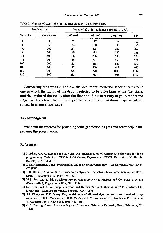
During the computational experiment, we observed an interesting property of the gravitational method. The bigger the radius of the initial drop, the smaller the number of steps to the first halt. In other words, if a dual feasible solution exists, we can find one faster (feasible to (1) in Section 2, which is in standard form), by making the radius of the drop large in the first stage. As explained in Section 2, we can make the radius of the initial drop arbitrarily large by taking the value of x$,t to be as large as we want. The results in Table 2 indicate that this leads to a speedier discovery of a dual feasible solution when one exists.

Table 1. Performance summary.

Variables Constraints CPU time in seconds

MINOS 5.0 GRAVITY 1

5 10 0.085 0.018

10 20 0.160 0.050

10 30 0.210 0.087

20 30 0.412 0.205

20 40 0.473 0.272

10 100 0.511 0.253

50 100 4.112 2.514

50 200 8.214 6.015

60 200 12.405 8.989

100 200 38.399 28.420

150 300 212.946 93.950

200 400 539.346 249.810


Table 2. Number of steps taken in the first stage in 10 different cases.

Problem size

Variables Constraints

30 50 30 50

50 100

50 100 75 100

75 100

100 200 100 200 150 300

150 300 _I-

Value of x,0+, in the initial point (0, . . . ,0,x!+ t)

l.OE+O9 l.OE+06 l.OE+03 1.0

52 97 101 102

54 90 90 82

111 205 252 212

99 193 237 233

136 208 249 268 115 221 258 262

182 458 643 660

177 460 618 672

295 770 1099 1144

282 713 948 1100

Considering the results in Table 2, the ideal radius reduction scheme seems to be one in which the radius of the drop is selected to be quite large at the first stage, and then reduced drastically after the first halt if it is necessary to go to the second stage. With such a scheme, most problems in our computational experiment are solved in at most two stages.

Acknowledgment

We thank the referees for providing some geometric insights and other help in im- proving the presentation.

References

PI

PI

[31

[41

[51

161

[71

I. Adler, M.G.C. Resende and G. Veiga, An implementation of Karmarkar’s algorithm for linear

programming, Tech. Rept. ORC 86-8, OR Center, Department of IEOR, University of California, Berkeley, CA (1986). K.M. Anstreicher, Linear programming and the Newton barrier flow, Yale University, New Haven,

CT (1987). E.R. Barnes, A variation of Karmarkar’s algorithm for solving linear programming problems, Math. Programming 36 (1986) 174-182. M.J. Best and K. Ritter, Linear Programming: Active Set Analysis and Computer Programs

(Prentice-Hall, Englewood Cliffs, NJ, 1985). S.S. Chiu and Y. Ye, Simplex method and Karmarkar’s algorithm: A unifying structure, EES

Department, Stanford University, Stanford, CA (1985). S.J. Chung and K.G. Murty, Polynomial bounded ellipsoid algorithm for convex quadratic programming, in: O.L. Mangasarian, R.R. Meyer and S.M. Robinson, eds., Nonlinear Programming 4 (Academic Press, New York, 1981) 439-485. G.B. Dantzig, Linear Programming and Extensions (Princeton University Press, Princeton, NJ, 1963).


[S] Y. Fathi, Computational complexity of LCP’s associated with positive definite symmetric matrices, Math. Programming 17 (1979) 335-344.

191 Y. Fathi, Comparative study of the ellipsoid algorithm and other algorithms for the nearest point

problem, Tech. Rept. 80-4, Department of Industrial and Operations Engineering, University of Michigan, Ann Arbor, MI (1980).

[IO] G. de Ghellinck and J.P. Vial, A polynomial Newton method for linear programming, Algorith- mica I (1986) 425-453.

[I I] E.G. Gilbert, D.W. Johnson and S.S. Keerthi, A fast procedure for computing the distances between complex objects in three space, Tech. Rept., Aerospace Engineering, University of Michigan,

Ann Arbor, MI (1986). 1121 P.E. Gill, W. Murrary, M.A. Saunders, J.A. Tomlin and M. Wright, On projected Newton barrier

methods for linear programming and an equivalence to Karmarkar’s projective method, Tech. Rept. SOL851 lR, Stanford University, Stanford, CA (1986).

[13] P.E. Gill, W. Murrary. M.A. Saunders, J.A. Tomlin and M. Wright, A note on nonlinear ap-

proaches to linear programming, Tech. Rept. SOL86-7, Stanford University, Stanford, CA (1986). [14] J.L. Coffin, Variable metric relaxation methods, Part I: A conceptual algorithm, Tech. Rept.

SOL81-16, Stanford University, Stanford, CA (1981). [I51 C.C. Gonzaga, An algorithm for solving linear programming problems in O(n3L) operations,

Department of Electrical Engineering and Computer Sciences, University of California, Berkeley, CA (1987).

[16] N. Karmarkar, A new polynomial-time algorithm for linear programming, Combinatorics 4 (1984) 373-395.

[ 171 M. Kojima, S. Mizuno and A. Yoshise, A primal-dual interior point algorithm for linear programming, Tech. Rept. B-188, Department of Information Sciences, Tokyo Institute of Technology, Tokyo (1987).

[18] O.L. Mangasarian, Nonlinear Programming (McGraw-Hill, New York, 1969).

1191 C.L. Monma, Recent breakthroughs in linear programming methods, Bell Communicatons Research, Murray Hill, NJ (1987).

[20] C.L. Monma and A.J. Morton, Computational experience with a dual affine variant of Kar- markar’s method for linear programming, Bell Communications Research, Murray Hill, NJ (1987).

[21] B.A. Murtagh and M.A. Saunders, MINOS 5.0 user’s guide, Rept. SOL83-20, Department of Operations Research, Stanford University, Stanford, CA (1983).

[22] K.G. Murty, Linear and Combinatorial Programming (Krieger Publishing Company Malabar, FL, 1976).

[23] K.G. Murty and Y. Fathi, A critical index algorithm for nearest point problems on simplicial cones, Math. Programming 23 (1982) 206-215.

[24] K.G. Murty, Linear Programming (Wiley, New York, 1983).

[25] K.G. Murty, The gravitational method for linear programming, OpSearch 23 (1986) 206-214. [26] K.G. Murty, Linear Complementarity, Linear and Nonlinear Programming (Heldermann, Berlin,

F.R.G., 1988).

1271 J. Renegar, A polynomial-time algorithm, based on Newton’s method, for linear programming, Tech. Rept. MSRI 07118-86, Mathematical Sciences Research Institute, Berkeley, CA (1986).

[28] J.B. Rosen, The gradient projection method for nonlinear programming, Part I: Linear constraints, SIAM J. Appl. Math. 8 (1960) 181-217.

[29] J.B. Rosen, The gradient projection method for nonlinear programming, Part II: Nonlinear constraints, SIAM J. Appl. Math. 9 (1961) 514-553.

[30] A. Tamura, H. Takehara, K. Fukuda, S. Fujishige and M. Kojima, A dual interior primal simplex

method for linear programming, Tech. Rept., Department of Information Sciences, Tokyo Institute of Technology, Tokyo (1987).

[31] M.J. Todd and B.P. Burrell, An extension of Karmarkar’s algorithm for linear programming using dual variables, Algorithmica 1 (1986) 409-424.


[32] R.J. Vanderbei, M.S. Meketon and B.A. Freedman, A modification of Karmarkar’s linear programming algorithm, Algorithmica 1 (1986) 395-408.

1331 D.R. Wilhelmsen, A nearest point algorithm for convex polyhedral cones and applications to positive linear approximation, Math. Comp. 30 (1976) 48-57.

[34] P. Wolfe, Algorithm for a least distance programming problem, Math. Programming Study 1 (1974) 190-205.

[35] P. Wolfe, Finding the nearest point in a polytope, Math. Programming 11 (1976) 128-149. [36] Y. Ye, Barrier-projection in projective algorithm for linear programming, Manuscript, Engineering

Economic Systems Department, Stanford University, Stanford, CA (1985). [37] Y. Ye, Cutting-objective and scaling method: ‘Simple’ polynomial algorithm for linear program-

ming, Manuscript, Engineering Economic Systems Department, Stanford University, Stanford, CA (1985).

[38] Y. Ye, and E. Tse, A polynomial-time algorithm for convex quadratic programming, Manuscript, Engineering Economic Systems Department, Stanford University, Stanford, CA (i986).

[39] Y. Ye, Karmarkar’s algorithm and the ellipsoid method, Oper. Res. Lett. 6(4) (1987) 177-182. [40] K. Zikan and R.W. Cottle, The box method for linear programming: Part I: Basic theory, Tech.

Rept. SOL87-6, Department of Operations Research, Stanford University, Stanford, CA (1987). [41] G. Zoutendijk, Methods of Feasible Directions: A Study in Linear and Nonlinear Programming

(Elsevier, New York, 1960). [42] G. Zoutendijk, Some algorithms based upon the principle of feasible directions, in: J.B. Rosen,

O.L. Mangasarian and K. Ritter, eds., Nonlinear Programming (Academic Press, London, 1970)

93-121. [43] G. Zoutendijk, Mathematical Programming Methods (North-Holland, Amsterdam, 1976).

THE STEEPEST DESCENT GRAVITATIONAL METHOD FOR LINEAR PROGRAMMING

Documents

Transcript of THE STEEPEST DESCENT GRAVITATIONAL METHOD FOR LINEAR PROGRAMMING