1

The statistical strength of nonlocality proofsWim van Dam, Richard D. Gill, Peter D. Grunwald,

Abstract— There exist numerous proofs of Bell’s theorem, stat-ing that quantum mechanics is incompatible with local realistictheories of nature. Here the strength of such nonlocality proofsis defined in terms of the amount of evidence against localrealism provided by the corresponding experiments. Statisticalconsiderations show that the amount of evidence should bemeasured by theKullback-Leibler or relative entropydivergence.

The statistical strength of the following proofs is determined:Bell’s original proof and Peres’ optimized variant of it, andproofs by Clauser-Horne-Shimony-Holt, Hardy, Mermin, andGreenberger-Horne-Zeilinger. The GHZ proof is at least fourand a half times stronger than all other proofs, while of thetwo-party proofs, the one of CHSH is the strongest.

Index Terms— nonlocality, Bell’s theorem, quantum correla-tions, Kullback-Leibler divergence

I. I NTRODUCTION

A PLETHORA of proofs exist of Bell’s theorem (“quantummechanics violates local realism”) encapsulated in in-

equalities and equalities of which the most celebrated are thoseof Bell [5], Clauser, Horne, Shimony and Holt (CHSH) [9],Greenberger, Horne and Zeilinger (GHZ) [16], Hardy [21],and Mermin [26]. Competing claims exist that one proof isstronger than another. For instance, a proof in which quantumpredictions having probabilities 0 or 1 only are involved, isoften said to be stronger than a proof that involves quantumpredictions of probabilities between 0 and 1. Other researchersargue that one should compare the absolute differences be-tween the probabilities that quantum mechanics predicts andthose that are allowed by local theories, and so on. The mainaim of this paper is to settle such questions once and forall: we formally define the strength of a nonlocality proofand we argue that our definition is the only one compatiblewith generally accepted notions in information theory andtheoretical statistics.

To see the connection with statistics, note first that amath-ematicalnonlocality proof shows that thepredictedprobabil-ities of quantum theory are incompatible with local realism.Such a proof can be implemented as anexperimental proofshowing thatphysical realityconforms to those predictions andhence too is incompatible with local realism. We are interestedin the strength of such experimental proofs, which should be

A preliminary version [11] of this paper, containing extensive backgroundmaterial, appeared on the arXiv preprint server in the quantum physics archiveas quant-ph/0307125.

Wim van Dam is with the Department of Computer Science, University ofCalifornia, Santa Barbara, Santa Barbara, CA 93106-5110 United States ofAmerica. Email: vandam@cs.ucsb.edu

Richard Gill is with the Mathematical Institute, University Utrecht, Bu-dapestlaan 6, NL-3584 CD Utrecht, The Netherlands. He is also at EURAN-DOM, Eindhoven, The Netherlands. Email: gill@math.uu.nl

Peter Grunwald is with the CWI, P.O. Box 94079, NL-1090 GB, TheNetherlands. He is also at EURANDOM, Eindhoven, The Netherlands. Email:pdg@cwi.nl

measured in statistical terms: how sure do we become that acertain theory is false, after observing a certain violation fromthat theory, in a certain number of experiments.

A. Our Game

We analyze the statistics of nonlocality proofs in terms of atwo-player game. The two players are the pro-quantum theoryexperimenter QM, and a pro-local realism theoretician LR.The experimenter QM is armed with a specific proof of Bell’stheorem. A given proof—BELL, CHSH, HARDY, MERMIN,GHZ—involves a collection of equalities and inequalitiesbetween various experimentally accessible probabilities. Theproof specifies a given quantum state (of a collection ofentangled qubits, for instance) and experimental settings (ori-entations of polarization filters or Stern-Gerlach devices). Alllocal realistic theories of LR will obey the (in)equalities,while the observations that QM will make when performingthe experiment (assuming that quantum mechanics is true)will violate these (in)equalities. The experimenter QM stillhas a choice of the probabilities with which the differentcombinations of settings will be applied, in a long sequenceof independent trials. In other words, he must still decidehow to allocate his resources over the different combinationsof settings. At the same time, the local realist can come upwith all kinds of different local realistic theories, predictingdifferent probabilities for the outcomes given the settings. Shemight put forward different theories in response to differentspecific experiments. Thus the quantum experimenter willchoose that probability distribution over his settings, for whichthe best local realistic model explains the dataworst, whencompared with the true (quantum mechanical) description.

B. Quantifying Statistical Strength - Past Approaches

How should we measure the statistical strength of a givenexperimental setup? In the past it was often simply said that thelargest deviation in the Bell inequality is attained with suchand such filter settings, and hence the experiment which isdone with these settings gives (potentially) the strongest proofof nonlocality. The argument is however not very convincing.One should take account of the statistical variability in finitesamples. The experiment that might confirm the largest abso-lute deviation from local realistic theories, might be subjectto the largest standard errors, and therefore be less convincingthan an experiment where a much smaller deviation can beproportionally much more accurately determined.

Alternatively, the argument has just been that with a largeenough sample size, even the smallest deviation between twotheories can be made firm enough. For instance, [26] has saidin the context of a particular example

2

“. . . to produce the conundrum it is necessary to runthe experiment sufficiently many times to establishwith overwhelming probability that the observedfrequencies (which will be close to 25% and 75%)are not chance fluctuations away from expectedfrequencies of 33% and 66%. (A million runs is morethan enough for this purpose). . . ”

We want to replace the words “sufficiently”, “overwhelming”,“more than enough” with something more scientific. (SeeExample 4 for our conclusion with respect to this.) And asexperiments are carried out that are harder and harder toprepare, it becomes important to design them so that theygive conclusive results with the smallest possible sample sizes.Initial work in this direction has been done by Peres [29]. Ourapproach is compatible with his, and extends it in a numberof directions—see Section VII-B.

C. Quantifying Statistical Strength - Our Approach

We measure statistical strength using an information-theoretic quantification, namely the Kullback-Leibler (KL)divergence (also known asinformation deficiencyor relativeentropy[10]). We show (Appendix III) that for large samples,all reasonable definitions of statistical strength that can befound in the statistical and information-theoretic literatureessentially coincide with our measure. For a given type ofexperiment, we consider the game in which the experimenterwants to maximize the divergence while the local theoristlooks for theories that minimize it. The experimenter’s gamespace is the collection of probability distributions over jointsettings, which we call in the sequel, for short, “settingdistributions”. (More properly, these are “joint setting distri-butions”.) The local realist’s game space is the space of localrealistic theories. This game defines an experiment, such thateach trial (assuming quantum mechanics is true) provides onaverage, the maximal support for quantum theory against thebest explanation that local realism can provide, at that settingdistribution.

D. Our Results - Numerical

We determined the statistical strength of five two-partyproofs: Bell’s original proof and Peres’ optimized variant of it,and the proofs of CHSH, Hardy, and Mermin. Among these,CHSH turns out to be the strongest by far. We also determinedthe strength of the three-party GHZ proof. Contrary to whathas sometimes been claimed (see Section VII), even the GHZexperiment has to be repeated a fair number of times before asubstantial violation of local realism is likely to be observed.Nevertheless, it is about 4.5 times stronger than the CHSHexperiment, meaning that, in order to observe the same supportfor QM and against LR, the CHSH experiment has to be runabout 4.5 times as often as the GHZ experiment — we provideprecise numbers in Section VI, Example 4.

E. Our Results - Mathematical

To find the (joint) setting distribution that optimizes thestrength of a nonlocality proof is a highly nontrivial com-putation. In the second part of this paper, we prove several

mathematical properties of our notion of statistical strength.These provide insights in the relation between local realistand quantum distributions that are interesting in their ownright. They also imply that determining statistical strengthof a given nonlocality proof may be viewed as a convexoptimization problem which can be solved numerically. Wealso provide a game-theoretic analysis involving minimax andmaximin KL divergences. This analysis allows us to shortcutthe computations in some important special cases.

F. Organization of This Paper

Section II gives a formal definition of what we mean by anonlocality proof and the corresponding experiment, as well asthe notation that we will use throughout the article. The kindsof nonlocality proofs that this article analyzes are describedin Section III, using the CHSH proof as a specific example;the other proofs are described in more detail in Appendices Iand II. The definition of the ‘statistical strength of a non-locality proof’ in terms of the Kullback-Leibler divergenceis presented in Section IV, along with some standard factsabout KL divergence and its role in hypothesis testing. Thestrength of a nonlocality proof is now well-defined, but itit is not yet clear how to compute it. In Section V wedevelop the mathematical techniques needed to perform thecomputations efficiently: we establish topological, analyticaland game-theoretic properties of statistical strength on whichour (mostly numerical, but sometimes exact) calculations arebased. This technical section may be skipped, since it isnot crucial for understanding the remainder of the paper.Section VI lists the results of our calculations of statisticalstrength for six well-known proofs (with additional detailsagain in Appendix II). The results are interpreted, discussedand compared in Section VII. In Section VIII we present fiveconjectures that are suggested by our results.

We defer all issues that require knowledge of the mathemati-cal aspects of quantum mechanics to the appendices. There weprovide more detailed information about the nonlocality proofswe analyzed, the relation of Kullback-Leibler divergence tohypothesis testing, and the proofs of the theorems we presentin the main text.

II. FORMAL SETUP

A basic nonlocality proof (“quantum mechanics violateslocal realism”) has the following ingredients. There are twopartiesA and B, who can each do a measurement on oneof two entangled qubits. They may each choose from twodifferent measurement settings. In each trial of the experiment,A andB randomly sample from the four different joint settingsand each observe one of two different binary outcomes, say“F” (false) and “T” (true). Quantum mechanics enables us tocompute the joint probability distribution of the outcomes, asa function of the measurement settings and of the joint stateof the two qubits. Thus possible design choices are: the stateof the qubits, the values of the settings; and the probabilitydistribution over the settings. More complicated experimentsmay involve more parties, more settings, and more outcomes.(We formalized the general set-up in [11]). In this text, we

3

focus primarily on the basic 2×2×2 case, which stands for“2 parties× 2 measurement settings per party× 2 outcomesper measurement setting”. Below we introduce notation for allingredients involved in nonlocality proofs.

A. Distribution of Settings

The random variableA denotes the measurement setting ofparty A and the random variableB denotes the measurementsetting of partyB. Both A and B take values in{1,2}. Theexperimenter QM will decide on the distributionσ of (A,B),giving the probabilities (and, after many trials of the experi-ment, the frequencies) with which each (joint) measurementsetting is sampled. Thissetting distributionσ is identified withits probability vectorσ := (σ11,σ12,σ21,σ22)∈ Σ, andΣ is theunit simplex inR4 defined by

Σ :={(σ11, . . . ,σ22) | ∑

a,b∈{1,2}σab = 1, for all a,b : σab≥ 0

}.

We useΣUC to denote the set of vectors representinguncor-related distributions inΣ. Formally, σ ∈ ΣUC if and only ifσab = (σa1 +σa2)(σ1b +σ2b) for all a,b∈ {1,2}.

B. Measurement Outcomes

The random variableX denotes the measurement outcomeof partyA and the random variableY denotes that of partyB.Both X andY take values in{T,F}, whereF means ‘false’and T means ‘true’. Thus, the statement ‘X = F,Y = T’ anddescribes the event that partyA observedF and partyB

observedT.The distribution of(X,Y) depends on the chosen setting

(a,b) ∈ {1,2}2. The state of the entangled qubits togetherwith the measurement settings determines four conditionaldistributionsQ11,Q12,Q21,Q22 for (X,Y), one for each jointmeasurement setting, whereQab is the distribution of(X,Y)given that measurement setting(a,b) has been chosen. Forexample,Qab(X = F,Y = T), abbreviated toQab(F,T), denotesthe probability that partyA observesF and partyB observesT, given that the device ofA is in settinga and the deviceof B is in setting b. According to QM, the total outcome(X,Y,A,B) of a single trial is then distributed asQσ , definedby Qσ (X = x,Y = y,A = a,B = b) := σabQab(X = x,Y = y).

C. Definition of a Nonlocality Proof and Corresponding Non-locality Experiments

A nonlocality proof for 2 parties, 2 measurement settingsper party, and 2 outcomes per measurement, is identifiedwith an entangled quantum state of two qubits (realized,by, e.g., two photons) and two measurement devices (e.g.,polarization filters) which each can be used in one of twodifferent measurement settings (polarization angles). Every-thing about the quantum state, the measurement devices, andtheir settings that is relevant for the probability distribution ofoutcomes of the corresponding experiment can be summarizedby the four distributionsQab of (X,Y), one for each (joint)setting (a,b) ∈ {1,2}2. Henceforth, we will simplyidentifya 2×2×2 nonlocality proof with the vector of distributionsQ := (Q11,Q12,Q21,Q22).

This definition can easily be extended in an entirely straight-forward manner to a situation with more than two parties, twosettings per party, or two outcomes per setting [11].

We call a nonlocality proofQ= (Q11,Q12,Q21,Q22) properif and only if it violates local realism, i.e. if there existsno local realist distributionπ (as defined below) such thatPab;π(·) = Qab(·) for all (a,b) ∈ {1,2}2.

For the corresponding 2× 2× 2 nonlocality experimentwe have to specify the setting distributionσ with whichthe experimenter QM samples the different settings(a,b).Thus, for a single nonlocality proofQ, QM can use differentexperiments (different inσ ) to verify Nature’s nonlocality.Each experiment consists of a series of trials, where—pertrial—the event(X,Y,A,B) occurs with probabilityQσ (X =x,Y = y,A = a,B = b) = σabQab(X = x,Y = y).

D. Local Realist Theories

The local realist (LR) may provide any ‘local’ theory shelikes to explain the results of the experiments.

Under such a theory it is possible to talk about “the outcomethat A would have observed, if she had used setting 1”,independently of which setting was used byB and indeedof whether or notA actually did use setting 1 or 2. Thuswe have four binary random variables, which we will callX1,X2, Y1 and Y2. As before, variables namedX correspond toA’s observations, and variables namedY correspond toB’sobservations. According to LR, each experiment determinesvalues for the four random variables(X1,X2,Y1,Y2). For a∈{1,2}, Xa ∈ {T,F} denotes the outcome that partyA wouldhave observed if the measurement setting ofA had beena.Similarly, for b∈ {1,2}, Yb ∈ {T,F} denotes the outcome thatpartyB would have observed if the measurement setting ofB

had beenb.A local theoryπ may be viewed as a probability distribution

for (X1,X2,Y1,Y2). Formally, we defineπ as a 16-dimensionalprobability vector with indices(x1,x2,y1,y2) ∈ {T,F}4. Bydefinition, Pπ(X1 = x1,X2 = x2,Y1 = y1,Y2 = y2) := πx1x2y1y2.For example,πFFFF denotes LR’s probability that, in allpossible measurement settings,A and B would both haveobservedF. The set of local theories can thus be identifiedwith the unit simplex inR16, which we will denote byΠ.

As discussed above, the quantum state of the entangledqubits determines four distributions over measurement out-comesQab(X = ·,Y = ·), one for each joint setting(a,b) ∈{1,2}2. Similarly, each LR theoryπ ∈ Π determines fourdistributionsPab;π(X = ·,Y = ·). These are the distributions,according to the local realist theoryπ, of the random variables(X,Y) given that setting(a,b) has been chosen. Thus, the valuePab;π(X = ·,Y = ·) is defined as the sum of four terms:

Pab;π(X = x,Y = y) := ∑x1,x2,y1,y2∈{T,F}

xa=x;yb=y

πx1x2y1y2.

We suppose that LR does not dispute the actual setting distri-butionσ which is used in the experiment, she only disputes theprobability distributions of the measurement outcomes giventhe settings. According to LR therefore, the outcome of asingle trial is distributed asPσ ;π defined byPσ ;π(X = x,Y =y,A = a,B = b) := σabPab;π(X = x,Y = y).

4

III. T HE NONLOCALITY PROOFS

In this paper we compute statistical strength for five (orsix, since we have two versions of Bell’s proof) celebratednonlocality proofs. In this section, we describe the general typeof reasoning by which these nonlocality proofs are established,using CHSH as a concrete example. Details on the other proofscan be found in Appendices I and II.

Let us interpret the measurement outcomesF andT in termsof Boolean logic, i.e.F is “false” and T is “true”. We canthen use Boolean expressions such asX2&Y2, which evaluatesto true whenever bothX2 andY2 evaluate to ‘true’, i.e. whenbothX2 = T andY2 = T. We derive the proofs by applying therule that if the eventX = T implies the eventY = T (in short“X =⇒ Y”), then Pr(X) ≤ Pr(Y). In similar vein, we willuse rules like Pr(X ∨Y) ≤ Pr(X) + Pr(Y) and 1−Pr(¬X)−Pr(¬Y)≤ 1−Pr(¬X∨¬Y) = Pr(X&Y).

As an aside we want to mention that the proofs of Bell,CHSH and Hardy all contain the following argument, whichcan be traced back to the nineteenth century logician GeorgeBoole (1815–1864) [8]. Consider four events such that¬B∩¬C∩¬D =⇒ ¬A. Then it follows thatA =⇒ B∪C∪D. Andfrom this, it follows that Pr(A)≤Pr(B)+Pr(C)+Pr(D). In theCHSH argument and the Bell argument, the events concernthe equality or inequality of one of theXi with one of theYj .In the Hardy argument, the events concern the joint equalityor inequality of one of theXi , one of theYj , and a specificvalueF or T.

Example 1 (The CHSH Argument):For the CHSH argu-ment one notes that the implication

[(X1 = Y1)&(X1 = Y2)&(X2 = Y1)] =⇒ (X2 = Y2)

is logically true, and hence(X2 6= Y2) =⇒ [(X1 6= Y1)∨ (X1 6=Y2)∨ (X2 6= Y1)] holds. As a result, local realism implies thefollowing “CHSH inequality”

Pr(X2 6= Y2)≤ Pr(X1 6= Y1)+Pr(X1 6= Y2)+Pr(X2 6= Y1),(1)

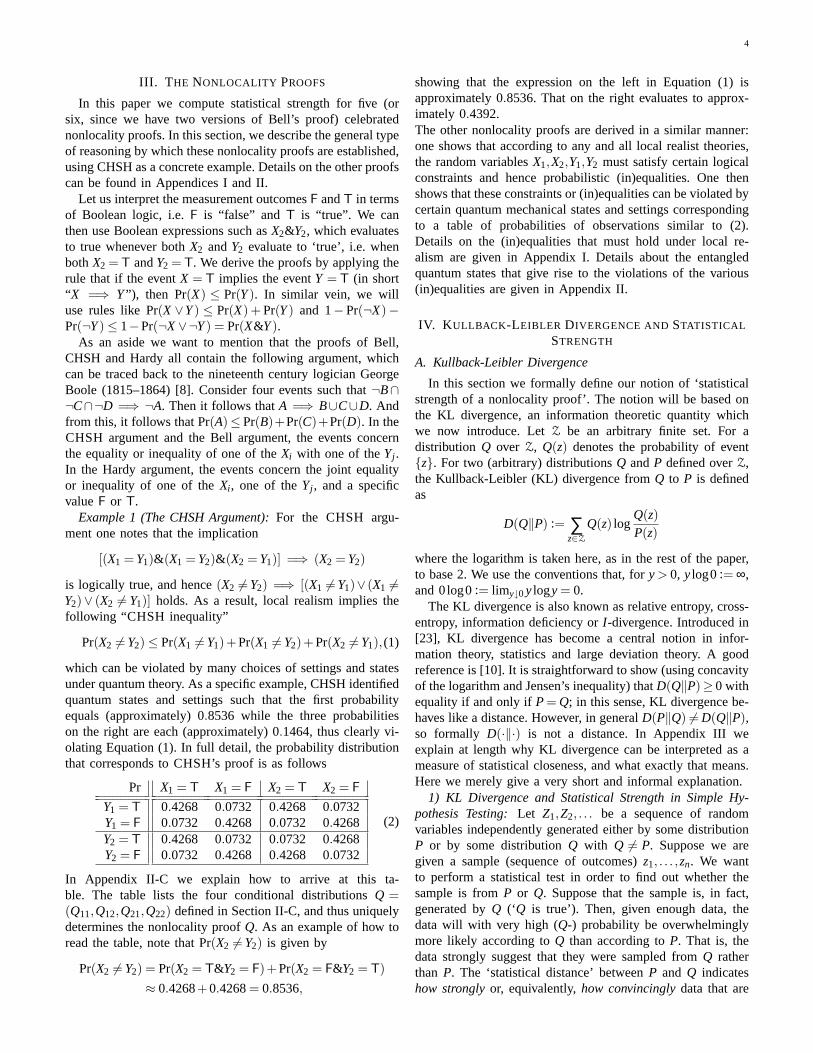
which can be violated by many choices of settings and statesunder quantum theory. As a specific example, CHSH identifiedquantum states and settings such that the first probabilityequals (approximately) 0.8536 while the three probabilitieson the right are each (approximately) 0.1464, thus clearly vi-olating Equation (1). In full detail, the probability distributionthat corresponds to CHSH’s proof is as follows

Pr X1 = T X1 = F X2 = T X2 = F

Y1 = T 0.4268 0.0732 0.4268 0.0732Y1 = F 0.0732 0.4268 0.0732 0.4268Y2 = T 0.4268 0.0732 0.0732 0.4268Y2 = F 0.0732 0.4268 0.4268 0.0732

(2)

In Appendix II-C we explain how to arrive at this ta-ble. The table lists the four conditional distributionsQ =(Q11,Q12,Q21,Q22) defined in Section II-C, and thus uniquelydetermines the nonlocality proofQ. As an example of how toread the table, note that Pr(X2 6= Y2) is given by

Pr(X2 6= Y2) = Pr(X2 = T&Y2 = F)+Pr(X2 = F&Y2 = T)≈ 0.4268+0.4268= 0.8536,

showing that the expression on the left in Equation (1) isapproximately 0.8536. That on the right evaluates to approx-imately 0.4392.The other nonlocality proofs are derived in a similar manner:one shows that according to any and all local realist theories,the random variablesX1,X2,Y1,Y2 must satisfy certain logicalconstraints and hence probabilistic (in)equalities. One thenshows that these constraints or (in)equalities can be violated bycertain quantum mechanical states and settings correspondingto a table of probabilities of observations similar to (2).Details on the (in)equalities that must hold under local re-alism are given in Appendix I. Details about the entangledquantum states that give rise to the violations of the various(in)equalities are given in Appendix II.

IV. K ULLBACK -LEIBLER DIVERGENCE AND STATISTICAL

STRENGTH

A. Kullback-Leibler Divergence

In this section we formally define our notion of ‘statisticalstrength of a nonlocality proof’. The notion will be based onthe KL divergence, an information theoretic quantity whichwe now introduce. LetZ be an arbitrary finite set. For adistribution Q over Z, Q(z) denotes the probability of event{z}. For two (arbitrary) distributionsQ andP defined overZ,the Kullback-Leibler (KL) divergence fromQ to P is definedas

D(Q‖P) := ∑z∈Z

Q(z) logQ(z)P(z)

where the logarithm is taken here, as in the rest of the paper,to base 2. We use the conventions that, fory> 0, ylog0:= ∞,and 0log0:= limy↓0ylogy = 0.

The KL divergence is also known as relative entropy, cross-entropy, information deficiency orI -divergence. Introduced in[23], KL divergence has become a central notion in infor-mation theory, statistics and large deviation theory. A goodreference is [10]. It is straightforward to show (using concavityof the logarithm and Jensen’s inequality) thatD(Q‖P)≥ 0 withequality if and only ifP= Q; in this sense, KL divergence be-haves like a distance. However, in generalD(P‖Q) 6= D(Q‖P),so formally D(·‖·) is not a distance. In Appendix III weexplain at length why KL divergence can be interpreted as ameasure of statistical closeness, and what exactly that means.Here we merely give a very short and informal explanation.

1) KL Divergence and Statistical Strength in Simple Hy-pothesis Testing:Let Z1,Z2, . . . be a sequence of randomvariables independently generated either by some distributionP or by some distributionQ with Q 6= P. Suppose we aregiven a sample (sequence of outcomes)z1, . . . ,zn. We wantto perform a statistical test in order to find out whether thesample is fromP or Q. Suppose that the sample is, in fact,generated byQ (‘Q is true’). Then, given enough data, thedata will with very high (Q-) probability be overwhelminglymore likely according toQ than according toP. That is, thedata strongly suggest that they were sampled fromQ ratherthan P. The ‘statistical distance’ betweenP and Q indicateshow stronglyor, equivalently,how convincinglydata that are

5

generated byQ will prove that they are fromQ rather thanP. It turns out that this notion of ‘statistical distance’ betweentwo distributions is precisely captured by the KL divergenceD(Q‖P), which can be interpreted asthe average amount ofsupport in favor of Q and against Pper trial. The larger theKL divergence, the larger the amount of support per trial. InAppendix III we explain at length what this means. For nowwe merely give an example: supposeD(Q‖P) = d for somed > 0, and we sample fromQ n times. Then we will observea sample that strongly indicates that it is very unlikely thatP generated the data. How unlikely? With(Q−) probabilityvery close to 1, our sample will makeP about as unlikely asthe hypothesis that a coin is fair if, aftern ·d throws, it haslanded ‘heads’ all the time—see Example 4 below.

2) KL Divergence and Statistical Strength in CompositeHypothesis Testing:Trying to infer whether a sample wasgenerated byQ or P is calledhypothesis testingin the statis-tical literature. A hypothesis issimpleif it consists of a singleprobability distribution. A hypothesis is calledcompositeif itconsists of asetof distributions. The composite hypothesis ‘P’should be interpreted as ‘there exists aP∈ P that generatedthe data’. Above, we related the KL divergence to statisticalstrength when testing two simple hypotheses against eachother. In this paper, the aim is to test two hypotheses, at leastone of which is composite. For concreteness, suppose we wantto test the distributionQ against the set of distributionsP. Inthis case, under some regularity conditions onP and Z, theelementP ∈ P that is closest in statistical divergence toQdetermines the statistical strength of the best test ofQ againstP. Therefore, for a set of distributionsP on Z we define (asis customary, [10])

D(Q‖P) := infP∈P

D(Q‖P).

Analogously toD(Q‖P), D(Q‖P) may be interpreted as theaverage amount of support in favor of Q and againstP pertrial , if data are generated according toQ.

In our case, QM claims that data are generated by thedistribution Qσ . LR claims that data are generated by someP∈ Pσ , wherePσ := {Pσ ;π : π ∈ Π}. HereQσ correspondsto a nonlocality proof equipped with setting distributionσ ,and Pσ is the set of probability distributions of all possiblelocal theories with the sameσ — see Section II. QM and LRagree to test the hypothesisQσ againstPσ . QM, who knowsthat data are really generated according toQσ , wants to selectσ in such a way that the average amount of support in favorof Q and againstP is maximized. LetΣ′ ⊆ Σ denote the setof all settingsσ that QM is allowed to choose from. Theprevious discussion suggests that QM should pick theσ ∈ Σ′thatmaximizes statistical strength D(Qσ‖Pσ ). In Appendix IIIwe show that this is (in some sense) also the optimal choiceaccording to statistical theory.

B. Formal Definition of Statistical Strength

We define ‘the statistical strength of nonlocality proofQ’in three different manners, depending on the freedom that weallow QM in determining the sampling probabilities of thedifferent measurement settings.

Definition 1 (Strength, Uniform Settings):When each measurement setting is sampled with equal prob-ability, the resulting strengthSUNI

Q is defined by

SUNIQ := D(Qσ◦‖Pσ◦) = inf

π∈ΠD(Qσ◦‖Pσ◦,π),

whereσ◦ denotes the uniform distribution over the settings.Definition 2 (Strength, Uncorrelated Settings):When the

experimenter QM is allowed to choose any distribution onmeasurement settings, as long as the distribution for eachparty is uncorrelated with the distributions of the otherparties, the resulting strengthSUC

Q is defined by

SUCQ := sup

σ∈ΣUC

D(Qσ‖Pσ ) = supσ∈ΣUC

infπ∈Π

D(Qσ‖Pσ ,π),

whereσ ∈ ΣUC denotes the use of uncorrelated settings.Definition 3 (Strength, Correlated Settings):When the ex-

perimenter QM is allowed to choose any distribution onmeasurement settings (including correlated distributions), theresulting strengthSCOR

Q is defined by

SCORQ := sup

σ∈ΣD(Qσ‖Pσ ) = sup

σ∈Σinf

π∈ΠD(Qσ‖Pσ ,π),

whereσ ∈ Σ denoted the use of correlated settings.Throughout the remainder of the paper, we sometimes abbre-viate the subscriptσ ∈ ΣUC to ΣUC, and π ∈ Π to Π. As weexplain in Section VII, we regard the definitionSUC

Q allowingmaximization over uncorrelated distributions as the ‘right’one. Henceforth, whenever we speak of ‘statistical strength’without further qualification, we refer toSUC

Q . Nevertheless, tofacilitate comparisons, in Section VI we list our results alsofor the two alternative definitions of statistical strength.

We have now completed our formal definition of statisticalstrength. The paper now branches into two parts, which canbe read separately: Section V is the mathematical part ofthis paper. Here we list some essential topological, analyticaland game-theoretic properties of our three notions of strength,needed for computing statistical strength in practice. The otherpart consists of Sections VI and all sections thereafter. InSection VI we calculate statistical strength for various non-locality proofs. The only mathematical result from Section Vthat is needed in Section VI and all sections thereafter is thefollowing reassuring fact (Theorem 1, Section V-A, part 2(c)):

Fact 1: SUNIQ ≤ SUC

Q ≤ SCORQ . Moreover,SUNI

Q > 0 if and onlyif Q is a proper nonlocality proof.

V. M ATHEMATICAL AND COMPUTATIONAL PROPERTIES OF

STATISTICAL STRENGTH

In this section we prove several mathematical propertiesof our three variations of statistical strength. Some of theseare interesting in their own right, giving new insights in therelation between distributions predicted by quantum theoryand local realist approximations of it. But their main purposeis to help us computeSUC

Q . We first establish some basicproperties of our three notions of strength (Section V-A).Section V-B provides a game-theoretic analysis which willhelp to computeSUC

Q very efficiently in certain special cases.Finally, in Section V-C we explicitly explain how to computeSUC

Q in practice.

6

A. Basic Properties

We proceed to list some essential properties ofSUNIQ ,SUC

Qand SCOR

Q . We say that “nonlocality proofQ is absolutelycontinuous with respect to local realist theoryπ” [13] ifand only if for all a,b∈ {1,2},x,y∈ {T,F}, it holds that ifQab(x,y) > 0 thenPab;π(x,y) > 0.

Theorem 1:Let Q be a given (not necessarily 2× 2× 2)nonlocality proof andΠ the (corresponding) set of local realisttheories.

1) Let U(σ ,π) := D(Qσ‖Pσ ;π), then:

a) For a 2×2×2 proof, we have that

U(σ ,π) = ∑a,b∈{1,2}

σabD(Qab‖Pab;π). (3)

Hence, the KL divergenceD(Qσ‖Pσ ;π) may alter-natively be viewed as the average KL divergencebetween the conditional distributions of(X,Y)given the setting(A,B), where the average is overthe setting. For a generalized nonlocality proof, theanalogous generalization of Equation (3) holds.

b) For fixedσ , U(σ ,π) is convex and lower semicon-tinuous onΠ, and continuous and differentiable onthe interior ofΠ.

c) If Q is absolutely continuous with respect to somefixed π, thenU(σ ,π) is linear inσ .

2) Let

U(σ) := infΠ

U(σ ,π), (4)

then

a) For all σ ∈ Σ, the infimum in Equation (4) isachieved for someπ∗.

b) The functionU(σ) is nonnegative, bounded, con-cave and continuous onσ .

c) If Q is not a proper nonlocality proof, then for allσ ∈Σ,U(σ) = 0. If Q is a proper nonlocality proof,thenU(σ) > 0 for all σ in the interior ofΣ.

d) For a 2 party, 2 measurement settings per partynonlocality proof, we further have that, even ifQis proper, then stillU(σ) = 0 for all σ on theboundary ofΣ.

3) Suppose thatσ is in the interior ofΣ, then:

a) Let Q be a 2× 2× 2 nonlocality proof. Supposethat Q is non-trivial in the sense that, for somea,b, Qab is not a point mass (i.e. 0< Qab(x,y) < 1for somex,y). Thenπ∗ ∈ Π achieves the infimumin Equation (4) if and only if the following 16(in)equalities hold:

∑a,b∈{1,2}

σabQab(xa,yb)

Pab;π∗(xa,yb)= 1 (5)

for all (x1,x2,y1,y2) ∈ {T,F}4 with π∗x1,x2,y1,y2> 0

and

∑a,b∈{1,2}

σabQab(xa,yb)

Pab;π∗(xa,yb)≤ 1 (6)

for all (x1,x2,y1,y2) ∈ {T,F}4 with π∗x1,x2,y1,y2= 0.

For generalized nonlocality proofs, the theoryπ∗ ∈Π achieves Equation (4) if and only if the corre-sponding analogues of Equations (5) and (6) bothhold.

b) Suppose thatπ∗ andπ◦ both achieve the infimumin Equation (4). Then for allx,y ∈ {T,F}, a,b ∈{1,2} with Qab(x,y) > 0, we havePab;π∗(x,y) =Pab;π◦(x,y) > 0. In words,π∗ and π◦ coincide inevery measurement setting for every measurementoutcome that has positive probability according toQσ , andQ is absolutely continuous with respect toπ∗ andπ◦.

The proof of this theorem is in Appendix IV-B.In general, infΠU(σ ,π) may be achieved for several, dif-

ferent π. By part 2 of the theorem, these must induce thesame four marginal distributionsPab;π . It also follows directlyfrom part 2 of the theorem that, for 2×2×2 proofs,SUC

Q :=supΣUC U(σ) is achieved for someσ∗ ∈ ΣUC, whereσ∗

ab > 0for all a,b∈ {1,2}.

B. Game-Theoretic Considerations

The following considerations will enable us to computeSUCQ

very efficiently in some special cases, most notably the CHSHproof.

We consider the following variation of our basic scenario.Suppose that, before the experiments are actually conducted,LR has to decide on asingle local theory π0 (rather thanthe setΠ) as an explanation of the outcomes that will beobserved. QM then gets to see thisπ, and can chooseσdepending on theπ0 that has been chosen. Since QM wants tomaximize the strength of the experiment, he will pick theσ

achieving supΣUC D(Qσ‖Pσ ;π0). In such a scenario, the ‘best’LR theory, minimizing statistical strength, is the LR theoryπ0

that minimizes, overπ ∈Π, supΣUC D(Qσ‖Pσ ;π). Thus, in thisslightly different setup, the statistical strength is determinedby

SUCQ := inf

ΠsupΣUC

D(Qσ‖Pσ ;π)

rather thanSUCQ := supΣUC infΠ D(Qσ‖Pσ ;π). Below we show

that SUCQ ≥ SUC

Q . As we already argued in Section VII, we con-sider the definitionSUC

Q to be preferable overSUCQ . Nevertheless,

it is useful to investigate under what conditionsSUCQ = S

UCQ .

Von Neumann’s famous minimax theorem of game theory [27]suggests that

supΣ∗

infΠ

D(Qσ‖Pσ ;π) = infΠ

supΣ∗

D(Qσ‖Pσ ;π), (7)

if Σ∗ is a convex subset ofΣ. Indeed, Theorem 2 below showsthat Equation (7) holds if we takeΣ∗ = Σ. Unfortunately,ΣUC

is not convex, and Equation (7) does not hold in generalfor Σ∗ = ΣUC, whence in generalSUC

Q 6= SUCQ . Nevertheless,

Theorem 3 provides some conditions under which Equation (7)does hold withΣ∗ = ΣUC. In Section V-C we put this fact touse in computingSUC

Q for the CHSH nonlocality proof. Butbefore presenting Theorems 2 and 3, we first need to introducesome game-theoretic terminology.

7

1) Game-Theoretic Definitions:Definition 4 (Statistical Game [14]):A statistical gameis

a triplet (A,B,L) where A and B are arbitrary sets andL :A×B→ R∪{−∞,∞} is a loss function. If

supα∈A

infβ∈B

L(α,β ) = infβ∈B

supα∈A

L(α,β ),

we say that the game hasvalue V with

V := supα∈A

infβ∈B

L(α,β ).

If for some (α∗,β ∗) ∈ A×B we have

For all α ∈ A: L(α,β ∗)≤ L(α∗,β ∗)For all β ∈ B: L(α∗,β )≥ L(α∗,β ∗)

then we call (α∗,β ∗) a saddle point of the game. It iseasily seen (Proposition 1, Appendix IV) that, ifα◦ achievessupα∈A infβ∈BL(α,β ) and β ◦ achieves infβ∈BL(α,β ) andthe game has valueV, then (α◦,β ◦) is a saddle point andL(α◦,β ◦) = V.

Definition 5 (Correlated Game):With each nonlocalityproof we associate a correspondingcorrelated game,whichis just the statistical game defined by the triple(Σ,Π,U),whereU : Σ×Π → R∪{∞} is defined by

U(σ ,π) := D(Qσ‖Pσ ;π).

By the definition above, if this game has a value then it isequal toV defined by

V := infΠ

supΣ

U(σ ,π) = supΣ

infΠ

U(σ ,π).

We call the gamecorrelatedbecause we allow distributionsσover measurement settings to be such that the probability thatpartyA is in settinga is correlated with (is dependent on) thesettingb of partyB. The fact that each correlated game has awell defined value is made specific in Theorem 2 below.

Definition 6 (Uncorrelated Game):Recall that we useΣUC

to denote the set of vectors representing uncorrelated distribu-tions in Σ. With each nonlocality proof we can associate thegame(ΣUC,Π,U) which we call the correspondinguncorre-lated game.

2) Game-Theoretic, Saddle Point Theorems:Theorem 2 (Saddle Point, Correlated Settings):For every

(generalized) nonlocality proof, the correlated game(Π,Σ,U)corresponding to it has a finite value, i.e. there exist a0 ≤ V < ∞ with infΠ supΣU(σ ,π) = V = supΣ infΠU(σ ,π).The infimum on the left is achieved for someπ∗ ∈ Π; thesupremum on the right is achieved for someσ∗ in Σ, so that(π∗,σ∗) is a saddle point.The proof of this theorem is in Appendix IV-C.2.

In the information-theoretic literature, several well-knownminimax and saddle point theorems involving the Kullback-Leibler divergence exist; we mention [22], [34]. However, allthese deal with settings that are substantially different fromours.

In the case where there are two parties and two measurementsettings per party, we can say a lot more.

Theorem 3 (Saddle Point,2×2×N Nonlocality Proofs):Fix any proper nonlocality proof based on 2 parties with

2 measurement settings per party and let(Σ,Π,U) and(ΣUC,Π,U) be the corresponding correlated and uncorrelatedgames, then:

1) The correlated game has a saddle point with valueV > 0.Moreover,

supΣUC

infΠ

U(σ ,π)≤ supΣ

infΠ

U(σ ,π) = V, (8)

infΠ

supΣUC

U(σ ,π) = infΠ

supΣ

U(σ ,π) = V. (9)

2) Let

Π∗ := {π : π achieves infΠ

supΣ

U(σ ,π)},

ΠUC∗ := {π : π achieves infΠ

supΣUC

U(σ ,π)},

then

a) Π∗ is non-empty.b) Π∗ = ΠUC∗.c) All π∗ ∈ Π∗ are ‘equalizer strategies’, i.e. for all

σ ∈ Σ we have the equalityU(σ ,π∗) = V.

3) The uncorrelated game has a saddle point if and only ifthere exists(π∗,σ∗), with σ∗ ∈ ΣUC, such that

a) π∗ achieves infΠU(σ∗,π).b) π∗ is an equalizer strategy.

If such (σ∗,π∗) exists, it is a saddle point.The proof of this theorem is in Appendix IV-C.3.

C. Computing Statistical Strength

We are now armed with the mathematical tools needed tocompute statistical strength. By convexity ofU(σ ,π) in π, wesee that for fixedσ , determiningD(Qσ‖Pσ ) = infΠU(σ ,π) isa convex optimization problem, which suggests that numericaloptimization is computationally feasible. Interestingly, it turnsout that computing infΠU(σ ,π) is formally equivalent tocomputing the maximum likelihood in a well-known statisticalmissing data problem. Indeed, we obtained our results by usinga ‘vertex direction algorithm’ [17], a clever numerical opti-mization algorithm specifically designed for statistical missingdata problems.

By concavity ofU(σ) as defined in Theorem 1, we see thatdeterminingSCOR

Q is a concave optimization problem. Thus,numerical optimization can again be performed. There aresome difficulties in computing the measureSUC

Q , since the setΣUC over which we maximize is not convex. Nevertheless,for the small problems (few parties, particles, measurementsettings) we consider here it can be done.

In some special cases, including CHSH, we can do all thecalculationsby handand do not have to resort to numericaloptimization. We do this by making an educated guess of theσ∗ achieving supΣUC D(Qσ‖Pσ ), and then verify our guessusing Theorem 1 and the game-theoretic tools developed inTheorem 3. This can best be illustrated using CHSH as anexample.

Example 2 (CHSH, continued):Consider the CHSH non-locality argument. The quantum distributionsQ, given in the

8

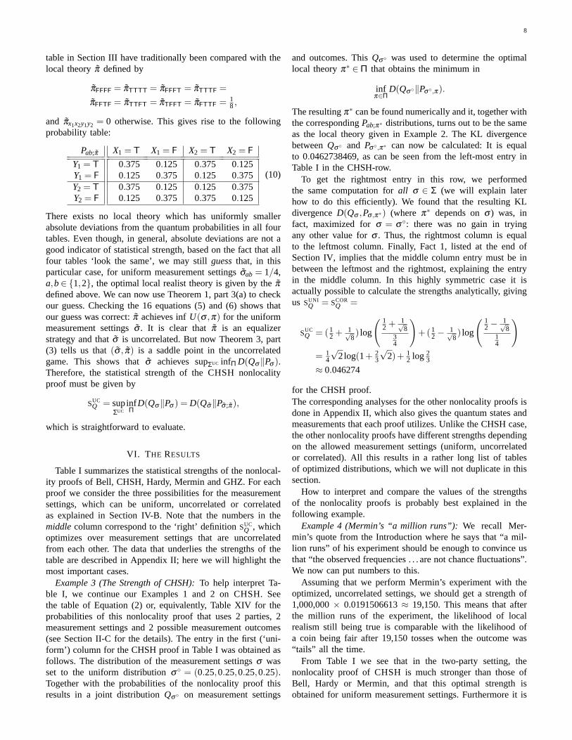
table in Section III have traditionally been compared with thelocal theoryπ defined by

πFFFF = πTTTT = πFFFT = πTTTF =πFFTF = πTTFT = πTFFT = πFTTF = 1

8,

and πx1x2y1y2 = 0 otherwise. This gives rise to the followingprobability table:

Pab;π X1 = T X1 = F X2 = T X2 = F

Y1 = T 0.375 0.125 0.375 0.125Y1 = F 0.125 0.375 0.125 0.375Y2 = T 0.375 0.125 0.125 0.375Y2 = F 0.125 0.375 0.375 0.125

(10)

There exists no local theory which has uniformly smallerabsolute deviations from the quantum probabilities in all fourtables. Even though, in general, absolute deviations are not agood indicator of statistical strength, based on the fact that allfour tables ‘look the same’, we may stillguessthat, in thisparticular case, for uniform measurement settingsσab = 1/4,a,b∈ {1,2}, the optimal local realist theory is given by theπ

defined above. We can now use Theorem 1, part 3(a) to checkour guess. Checking the 16 equations (5) and (6) shows thatour guess was correct:π achieves infU(σ ,π) for the uniformmeasurement settingsσ . It is clear that π is an equalizerstrategy and thatσ is uncorrelated. But now Theorem 3, part(3) tells us that(σ , π) is a saddle point in the uncorrelatedgame. This shows thatσ achieves supΣUC infΠ D(Qσ‖Pσ ).Therefore, the statistical strength of the CHSH nonlocalityproof must be given by

SUCQ = sup

ΣUC

infΠ

D(Qσ‖Pσ ) = D(Qσ‖Pσ ;π),

which is straightforward to evaluate.

VI. T HE RESULTS

Table I summarizes the statistical strengths of the nonlocal-ity proofs of Bell, CHSH, Hardy, Mermin and GHZ. For eachproof we consider the three possibilities for the measurementsettings, which can be uniform, uncorrelated or correlatedas explained in Section IV-B. Note that the numbers in themiddlecolumn correspond to the ‘right’ definitionSUC

Q , whichoptimizes over measurement settings that are uncorrelatedfrom each other. The data that underlies the strengths of thetable are described in Appendix II; here we will highlight themost important cases.

Example 3 (The Strength of CHSH):To help interpret Ta-ble I, we continue our Examples 1 and 2 on CHSH. Seethe table of Equation (2) or, equivalently, Table XIV for theprobabilities of this nonlocality proof that uses 2 parties, 2measurement settings and 2 possible measurement outcomes(see Section II-C for the details). The entry in the first (‘uni-form’) column for the CHSH proof in Table I was obtained asfollows. The distribution of the measurement settingsσ wasset to the uniform distributionσ◦ = (0.25,0.25,0.25,0.25).Together with the probabilities of the nonlocality proof thisresults in a joint distributionQσ◦ on measurement settings

and outcomes. ThisQσ◦ was used to determine the optimallocal theoryπ∗ ∈ Π that obtains the minimum in

infπ∈Π

D(Qσ◦‖Pσ◦,π).

The resultingπ∗ can be found numerically and it, together withthe correspondingPab;π∗ distributions, turns out to be the sameas the local theory given in Example 2. The KL divergencebetweenQσ◦ and Pσ◦,π∗ can now be calculated: It is equalto 0.0462738469, as can be seen from the left-most entry inTable I in the CHSH-row.

To get the rightmost entry in this row, we performedthe same computation forall σ ∈ Σ (we will explain laterhow to do this efficiently). We found that the resulting KLdivergenceD(Qσ ,Pσ ,π∗) (where π∗ depends onσ ) was, infact, maximized forσ = σ◦: there was no gain in tryingany other value forσ . Thus, the rightmost column is equalto the leftmost column. Finally, Fact 1, listed at the end ofSection IV, implies that the middle column entry must be inbetween the leftmost and the rightmost, explaining the entryin the middle column. In this highly symmetric case it isactually possible to calculate the strengths analytically, givingus SUNI

Q = SCORQ =

SUCQ = (1

2 + 1√8) log

( 12 + 1√

834

)+(1

2 −1√8) log

( 12 −

1√8

14

)= 1

4

√2log(1+ 2

3

√2)+ 1

2 log 23

≈ 0.046274

for the CHSH proof.The corresponding analyses for the other nonlocality proofs isdone in Appendix II, which also gives the quantum states andmeasurements that each proof utilizes. Unlike the CHSH case,the other nonlocality proofs have different strengths dependingon the allowed measurement settings (uniform, uncorrelatedor correlated). All this results in a rather long list of tablesof optimized distributions, which we will not duplicate in thissection.

How to interpret and compare the values of the strengthsof the nonlocality proofs is probably best explained in thefollowing example.

Example 4 (Mermin’s “a million runs”): We recall Mer-min’s quote from the Introduction where he says that “a mil-lion runs” of his experiment should be enough to convince usthat “the observed frequencies . . . are not chance fluctuations”.We now can put numbers to this.

Assuming that we perform Mermin’s experiment with theoptimized, uncorrelated settings, we should get a strength of1,000,000× 0.0191506613≈ 19,150. This means that afterthe million runs of the experiment, the likelihood of localrealism still being true is comparable with the likelihood ofa coin being fair after 19,150 tosses when the outcome was“tails” all the time.

From Table I we see that in the two-party setting, thenonlocality proof of CHSH is much stronger than those ofBell, Hardy or Mermin, and that this optimal strength isobtained for uniform measurement settings. Furthermore it is

9

TABLE I

STRENGTHS OFVARIOUS NONLOCALITY PROOFS

Strength Uniform SUNIQ UncorrelatedSUC

Q CorrelatedSCORQ

Original BELL 0.0141597409 0.0158003672 0.0169800305Optimized BELL 0.0177632822 0.0191506613 0.0211293952

CHSH 0.0462738469 0.0462738469 0.0462738469HARDY 0.0278585182 0.0279816333 0.0280347655

MERMIN 0.0157895843 0.0191506613 0.0211293952GHZ 0.2075187496 0.2075187496 0.4150374993

clear that the three-party proof of GHZ is four and a halftimes stronger than all the two-party proofs.

We also note that the nonlocality proof of Mermin—inthe case of non-uniform settings—is equally strong as theoptimized version of Bell’s proof. The setting distributionstables in Appendix II-E shows why this is the case: the optimalsetting distribution for Mermin exclude one setting onA’sside, and one setting onB’s side, thus reducing Mermin’sproof to that of Bell. One can view this is as an exampleof how a proof that is easier to understand (Mermin) is notnecessarily stronger than one that has more subtle arguments(Bell).

We also see that in general, except for CHSH’s proof,uniform setting distributions do not give the optimal strengthof a nonlocality proof. Rather, the experimenter obtains moreevidence for the nonlocality of nature by employing samplingfrequencies that are biased towards those settings that are morerelevant for the nonlocality proof.

VII. I NTERPRETATION ANDDISCUSSION

A. Is our definition of statistical strength the right one?

We can think of two objections against our definition ofstatistical strength. First, we may wonder whether the KLdivergence is really the right measure to use. Second, assumingthat KL divergence is the right measure, is our game-theoreticset-up justified? We treat both issues in turn.

1) Is Kullback-Leibler divergence justified?:We can seetwo possible objections against KL divergence: (1) differentstatistical paradigms such as the ‘Bayesian’ and ‘frequentist’paradigm define ‘amount of support’ in different manners (Ap-pendix III); (2) ‘asymptopia’: KL divergence is an inherentlyasymptotic notion.

These two objections are inextricably intertwined: there ex-ists no non-asymptotic measure which would (a) be acceptableto all statisticians; (b) would not depend on prior consid-erations, such as a ‘prior distribution’ for the distributionsinvolved in the Bayesian framework, and a pre-set significancelevel in the frequentist framework. Thus, since we consider itmost important to arrive at a generally acceptable and objectivemeasure, we decided to opt for the KL divergence. We addhere that even though this notion is asymptotic, it can be usedto provide numerical bounds on the actual, non-asymptoticamount of support provided on each trial, both in Bayesian

and in frequentist terms. We have not pursued this option anyfurther here.

2) Game-Theoretic Justification:There remains the ques-tion of whether to preferSUNI

Q , SCORQ or, as we do,SUC

Q . Theproblem with SUNI

Q is that, for any given combination ofnonlocality proofQ and local theoryπ, some settings mayprovide, on average, more information about the nonlocalityof nature than others. This is evident from Table I. We see noreason for the experimenter not to exploit this.

On the other hand, allowing QM to usecorrelated dis-tributions makes QM’s case much weaker: LR might nowargue that there is some hidden communication between theparties. Since QM’s goal is to provide an experiment that isas convincing as possible to LR, we do not allow for thissituation. Thus, among the three definitions considered,SUC

Qseems to be the most reasonable one. Nevertheless, one maystill argue thatnone of the three definitions of strength arecorrect: they all seem unfavorable to QM, since we allow LRto adjust his theory to whatever frequency of measurementsettings QM is going to use. In contrast, our definition doesnot allow QM to adjust his setting distribution to LR’s choice(which would lead to strength defined as infsup rather thansupinf, Section V-B). The reason why we favor LR in thisway is that the quantum experimenters QM should try toconvince LR that nature is nonlocalin a setting about whichLR cannot complain. Thus, if LR wants to entertain severallocal theories at the same time, or wants to have a look atthe probabilitiesσab before the experiment is conducted, QMshould allow him to do so—he will still be able to convinceLR, even though he may need to repeat the experiment a fewmore times. Nevertheless, in developing clever strategies forcomputing SUC

Q , it turns out to be useful to investigate theinfsup scenario in more detail. This was done in Section V-B.

Summarizing, our approach is highly nonsymmetric be-tween quantum mechanics and local realism. There is onlyone quantum theory, and QM believes in it, but he must arm

10

himself against any and all local realists.1

B. Related Work by Peres

Earlier work in our direction has been done by Peres [29]who adopts a Bayesian approach. Peres implicitly uses thesame definition of strength of nonlocality proofs as we do here,after merging equal probability joint outcomes of the experi-ment. Our work extends his in several ways; most importantly,we allow the experimentalist to optimize her experimentalsettings, whereas Peres assumes particular (usually uniform)distributions over the settings. Peres determines LR’s besttheory by an inspired guess. The proofs he considers haveso many symmetries, that the best LR theory has the sameequal probability joint outcomes as the QM experiment, thereduced experiment is binary, and his guess always gives theright answer. But his strategy would not work for, e.g., theHardy proof, which is less symmetric.

Peres starts out with a nonlocality proofQσ to be testedagainst local theoryPσ ;π , for some fixed distributionσ . Peresthen defines theconfidence depressing factor for n trials. Infact, Peres rediscovers the notion of KL divergence, since astraightforward calculation shows that for largen,

D(Qσ‖Pσ ;π) =1n

log(confidence depressing factor). (11)

For any given largen, the larger the confidence depressingfactor forn, the more evidence againstPσ ;π we are likely to geton the basis ofn trials. Thus, when comparing a fixed quantumexperiment (with fixedσ ) Qσ to a fixed local theoryPσ ;π ,Peres’ notion of strength is equivalent to ours . Peres then goeson to say that, when comparing a fixed quantum experimentQσ to the corresponding set ofall local theoriesPσ , we mayexpect that LR will choose the local theory with the leastconfidence depressing factor, i.e. the smallest KL divergenceto Qσ . Thus, whenever Peres chooses uniformσ , his notionof strength corresponds to ourSUNI

Q , represented in the firstcolumn of Table I. In practice, Peres chooses an intuitiveσ ,which is usually, but not always uniform in our sense. Forexample, in the GHZ scenario, Peres implicitly assumes thatonly those measurement settings are used that correspond tothe probabilities (all 0 or 1) appearing in the GHZ-inequality(12), Appendix I-D. Thus, his experiment corresponds to auniform distribution on those four settings. Interestingly, sucha distribution on settings isnot allowed under our definitionof strengthSUC

Q , since it makes the probability of the setting atparty A dependent on (correlated with) the other settings. Thisexplains that Peres obtains a larger strength for GHZ than wedo: he obtains log0.75−n = 0.4150. . .n, which corresponds

1Some readers might wonder what would happen if one would replacethe D(Q‖P) in our analysis byD(P‖Q). In short, D(P‖Q) quantifies howstrongly the predictions of quantum mechanics disagree with the outcomesof a classical systemP. Hence such an analysis would be useful if one hasto prove that the statistics of a local realistic experiment (say, a network ofclassically communicating computers) are not in correspondence with certainpredictions of quantum mechanics. The minimax solution of the game basedon D(P‖Q) provides a value ofQ which QM should specify as part of achallenge to LR to reproduce quantum predictions with LR’s theory. Withthis challenge, the computer simulation using LR’s theory can be run in asshort as possible amount of time, before giving sufficient evidence that LRhas failed.

to our SCORQ : the uniform distribution on the restricted set

of settings appearing in the GHZ proof turns out to be theoptimum over all distributions on measurement settings.

Our approach may be viewed as an extension of Peres’ inseveral ways. First, we relate his confidence depressing factorto the Kullback-Leibler divergence and we argue that this isthe right measure to use not just from a Bayesian point ofview, but also from an information-theoretic point of view andthe standard, ‘orthodox’ frequentist statistics point of view.Second, we extend his analysis to non-uniform distributionsσ over measurement settings and show that in some cases,substantial statistical strength can be gained if QM usesnon-uniform sampling distributions. Third, we give a game-theoretic treatment of the maximization ofσ and develop thenecessary mathematical tools to enable fast computations ofstatistical strength. Fourth, whereas Peres finds the best LRtheory by cleverly guessing, we show the search for this theorycan be performed automatically.

C. Which nonlocality proof is strongest and what does itmean?

1) Caveat: statistical strength is not the whole story:Firstof all, we stress that statistical strength is by no means the onlyfactor in determining the ‘goodness’ of a nonlocality proof andits corresponding experiment. Various other aspects also comeinto play, such as: how easy is it to prepare certain types ofparticles in certain states? Can we arrange to have the timeand spatial separations which are necessary to make the resultsconvincing? Can we implement the necessary random changesin settings per trial, quickly enough? Our notion of strengthneglects all these important practical aspects.

2) Comparing GHZ and CHSH:GHZ is the clear winneramong all proofs that we investigated, being about 4.5 timesstronger than CHSH, the strongest two-party proof that wefound. This means that, to obtain a given level of supportfor QM and against LR, the optimal CHSH experiment hasto be repeated about 4.5 times as often as the optimal GHZexperiment.

On the other hand, the GHZ proof is much harder to prepareexperimentally. In light of the reasoning above, and assumingthat both CHSH and GHZ can be given a convincing ex-perimental implementation, it may be the case that repeatingthe CHSH experiment 4.5× n times is much cheaper thanrepeating GHZn times.

3) Nonlocality ‘without inequality’?:The GHZ proof wasthe first of a new class of proofs of Bell’s theorem, “withoutinequalities”. It specifies a state and collection of settings,such that all QM probabilities are zero or one, while thisis impossible under LR. The QM probabilities involved arejust the probabilities of the four events in Equation (12),Appendix I-D. The fact that all these must be either 0 or 1 hasled some to claim that the corresponding experiment has to beperformed only once in order to rule out local realism2. As hasbeen observed before [29], this is not the case. This can be seen

2Quoting [29], “The list of authors [claiming that a single experiment issufficient to invalidate local realism] is too long to be given explicitly, and itwould be unfair to give only a partial list.”

11

immediately if we let LR adopt the uniform distribution on allpossible observations. Then, although QM is correct, no matterhow often the experiment is repeated, the resulting sequenceof observations does not have zero probability under LR’slocal theory — simply becauseno sequence of observationshas probability 0 under LR’s theory. We can only decide thatLR is wrong on a statistical basis: the observations aremuchmore likelyunder QM than under LR. This happens even if,instead of using the uniform distribution, LR uses the localtheory that is closest in KL divergence to theQ induced bythe GHZ scenario. The reason is that there exists a positiveε such that any local realist theory which comes withinε

of all the equalities but one, is forced to deviate by morethan ε in the last. Thus, accompanying the GHZ style proofwithout inequalities, is an impliedinequality, and it is thislatter inequality that can be tested experimentally.

VIII. F UTURE EXTENSIONS AND CONJECTURES

The purpose of our paper has been to objectively comparethe statistical strength of existing proofs of Bell’s theorem.The tools we have developed, can be used in many furtherways.

Firstly, one can take a given quantum state, and ask thequestion, what is the best experiment which can be donewith it. This leads to a measure of statistical nonlocality ofa given joint state, whereby one is optimizing (in the outeroptimization) not just over setting distributions, but also overthe settings themselves, and even over the number of settings.

Secondly, one can take a given experimental type, forinstance: the 2× 2× 2 type, and ask what is the best state,settings, and setting distribution for that type of experiment?This comes down to replacing the outer optimization oversetting distributions, with an optimization over states, settings,and setting distribution.

Using numerical optimization, we were able to analyze anumber of situations, leading to the following conjectures.

Conjecture 1:Among all 2× 2× 2 proofs, and allowingcorrelated setting distributions, CHSH is best.

Conjecture 2:Among all 3× 2× 2 proofs, and allowingcorrelated setting distributions, GHZ is best.

Conjecture 3:The best experiment with the Bell singletstate is the CHSH experiment.In [1] Acın et al. investigated the natural generalization ofCHSH type experiments to qutrits. Their main interest was theresistance of a given experiment to noise, and to their surprisethey discovered in the 2× 2× 3 case, that a less entangledstate was more resistant to noise than the maximally entangledstate. After some preliminary investigations, we found that thata similar experiment with aneven less entangledstate gives astronger nonlocality experiment.

Conjecture 4:The strongest possible 2×2×3 nonlocalityproof has statistical strength 0.077, and it uses the bipartitestate≈ 0.6475|1,1〉+0.6475|2,2〉+0.4019|3,3〉.If true, this conjecture is in remarkable contrast with whatappears to be the strongest possible 2× 2× 3 nonlocalityproof that uses the maximally entangled state(|1,1〉+ |2,2〉+|3,3〉)/

√3, which has a statistical strength of only 0.058.

Conjecture 4 suggests that it is not always the case that aquantum state with more ‘entropy of entanglement’ [6] willalways give a stronger nonlocality proof. Rather, it seems thatentanglement and statistical nonlocality are different quan-tities. One possibility however is that the counterintuitiveresults just mentioned would disappear if one could do jointmeasurements on several pairs of entangled qubits, qutrits,or whatever. A regularized measure of nonlocality of a givenstate, would be the limit fork→∞, of the strength of the bestexperiment based onk copies of the state (where the partiesare allowed to make joint measurements onk systems at thesame time), divided byk. One may conjecture for instance thatthe best experiment based on two copies of the Bell singletstate is more than twice as good as the best experiment basedon single states. That would be a form of “superadditivity ofnonlocality”, quite in line with other forms of superadditivitywhich is known to follow from entanglement.

Conjecture 5:There is an experiment on pairs of Bellsinglets, of the 2×4×4 type, more than twice as strong asCHSH, and involving joint measurements on the pairs.

IX. A CKNOWLEDGMENTS

The authors are very grateful to Piet Groeneboom forproviding us with the programs [17] needed to computeinfP∈P D(Q‖P), and helping us to adjust them for our pur-poses.

The authors would like to thank EURANDOM for financialsupport. Part of this research was performed while PeterGrunwald was visiting the University of California at SantaCruz (UCSC). The visit was funded by NWO (the NetherlandsOrganization for Scientific Research) and the Applied Mathand Computer Science Departments of UCSC. Wim van Dam’swork was partly supported by funds provided by the U.S. De-partment of Energy (DOE) and cooperative research agreementDF-FC02-94ER40818, by a CMI postdoctoral fellowship, andby an earlier HP/MSRI fellowship. Richard Gill’s researchwas partially funded by project RESQ (IST-2001-37559) ofthe IST-FET programme of the European Union. Richard Gillis grateful for the hospitality of the Quantum Probabilitygroup at the department of mathematics of the Universityof Greifswald, Germany. His research there was supportedby European Commission grant HPRN-CT-2002-00279, RTNQP-Applications. This work was also supported in part by theEuropean Union’s PASCAL Network of Excellence, IST-2002-506778.

REFERENCES

[1] A. Acın, T. Durt, N. Gisin, J.I. Latorre, “Quantum non-locality in twothree-level systems”,Physical Review A,Volume 65, 052325, 2002.

[2] R.R. Bahadur, “An optimal property of the likelihood ratio statistic”, InProceedings of the Fifth Berkeley Symposium on Mathematical Statisticsand Probability,Volume 1, pp. 13–26, 1967.

[3] V. Balasubramanian, “A Geometric Formulation of Occam’s Razor forInference of Parametric Distributions”, arXiv:adap-org/9601001, 1996.

[4] A. Barron and T. Cover, “Minimum complexity density estimation”,IEEE Transactions on Information Theory,Volume 37(4), pp. 1034–1054, 1991.

[5] J.S. Bell, “On the Einstein-Podolsky-Rosen paradox”,Physics, Vol-ume 1, pp. 195–200, 1964.

12

[6] C.H. Bennett, H.J. Bernstein, S. Popescu and B. Schumacher, “Concen-trating partial entanglement by local operations”,Physical Review A,Volume 53, No. 4, pp. 2046–2052, 1996.

[7] J.M. Bernardo and A.F.M. Smith,Bayesian theory,John Wiley, 1994.[8] G. Boole,An Investigation of the Laws of Thought (on which are founded

the mathematical theories of logic and probabilities),MacMillan andCo., Cambridge, 1854. Reprinted by Dover, 1951.

[9] J.F. Clauser, M.A. Horne, A. Shimony, and R.A. Holt, “Proposed exper-iment to test local hidden-variable theories”,Physical Review Letters,Volume 23, pp. 880–884, 1969.

[10] T.M. Cover and J.A. Thomas,Elements of Information Theory,WileyInterscience, New York, 1991.

[11] W. van Dam, R.D. Gill, and P.D. Grunwald, “The statistical strength ofnonlocality proofs”, arXiv:quant-ph/0307125, 2003.

[12] W. Feller, An Introduction to Probability Theory and Its Applications,Wiley, Volume 1, third edition, 1969.

[13] W. Feller, An Introduction to Probability Theory and Its Applications,Wiley, Volume 2, third edition, 1969.

[14] T.S. Ferguson,Mathematical Statistics — a decision-theoretic approach,Academic Press, 1967.

[15] T.L. Fine, Theories of Probability,Academic Press, 1973.[16] D.M. Greenberger, M. Horne, and A. Zeilinger, “Going beyond Bell’s

theorem”, In M. Kafatos, editor,Bell’s Theorem, Quantum Theory, andConceptions of the Universe,pp. 73–76, Kluwer, Dordrecht, 1989.

[17] P. Groeneboom, G. Jongbloed, and J.A. Wellner “Vertex direction al-gorithms for computing nonparametric function estimates in mixturemodels”, arXiv:math.ST/0405511, submitted, 2003.

[18] P. Groeneboom and J. Oosterhoff, “Bahadur efficiency and probabilitiesof large deviations”,Statistica Neerlandica,Volume 31, pp. 1–24, 1977.

[19] P.D. Grunwald, The Minimum Description Length Principle and Rea-soning under Uncertainty,PhD thesis, University of Amsterdam, TheNetherlands, October 1998. Available as ILLC Dissertation Series 1998-03.

[20] P. Grunwald and A.P. Dawid, ”Game theory, maximum entropy, min-imum discrepancy, and robust Bayesian decision theory”,Annals ofStatistics,Volume 32(4), pp. 1367–1433, August 2004.

[21] L. Hardy, “Nonlocality for two particles without inequalities for almostall entangled states”,Physical Review Letters,Volume 71, pp. 1665–1668, 1993.

[22] D. Haussler, “A general minimax result for relative entropy”,IEEETransactions on Information Theory,Volume 43(4), pp. 1276–1280,1997.

[23] S. Kullback and R.A. Leibler, “On information and sufficiency”,Annalsof Mathematical Statistics,Volume 22, pp. 76–86, 1951.

[24] P.M. Lee, Bayesian Statistics — an introduction,Arnold & OxfordUniversity Press, 1997.

[25] M. Li and P.M.B. Vitanyi, An Introduction to Kolmogorov Complexityand Its Applications,(revised and expanded Second edition), New York,Springer-Verlag, 1997.

[26] N.D. Mermin, “Quantum mysteries for anyone”,Journal of Philosophy,Volume 78, pp. 397–408, 1981.

[27] J. Von Neumann, “Zur Theorie der Gesellschaftsspiele”,MathematischeAnnalen,Volume 100, pp. 295–320, 1928.

[28] A. Peres,Quantum Theory: Concepts and Methods,Fundamental Theo-ries of Physics, Volume 57, Kluwer Academic Publishers, 1995.

[29] A. Peres, “Bayesian analysis of Bell inequalities”,Fortschritte derPhysik,Volume 48, pp. 531–535, 2000.

[30] E. Posner, “Random coding strategies for minimum entropy”,IEEETransactions on Information Theory,Volume 21, pp. 388–391, 1975.

[31] J.A. Rice, Mathematical Statistics and Data Analysis,Duxbury Press,1995.

[32] J. Rissanen,Stochastic Complexity in Statistical Inquiry,World ScientificPublishing Company, 1989.

[33] R.T. Rockafellar,Convex Analysis,Princeton University Press, Princeton,New Jersey, 1970.

[34] F. Topsøe, “Information-theoretical optimization techniques”,Kyber-netika,Volume 15(1), 1989.

[35] V. Vapnik, Statistical Learning Theory,John Wiley, 1998.

APPENDIX ITHE NONLOCALITY ARGUMENTS

In this Appendix we present the inequalities and logicalconstraints that must hold under local realism yet can beviolated under quantum mechanics. The specific quantum

states chosen to violate these inequalities, as well as the closestpossible (in the KL divergence sense) local theories are listedin Appendix II.

A. Arguments of Bell and CHSH

CHSH’s argument was described in Example 1. By exactlythe same line of reasoning as used in obtaining the CHSHinequality (1), one also obtains Bell’s inequality

Pr(X1 = Y1)≤ Pr(X2 6= Y2)+Pr(X2 6= Y1)+Pr(X1 +Y2).

See Sections II-A and II-B for how this inequality can beviolated.

B. Hardy’s Argument

Hardy noted the following: if(X2&Y2) is true, and(X2 =⇒Y1) is true, and(Y2 =⇒ X1) is true, then(X1&Y1) is true. Thus(X2&Y2) implies:¬(X2 =⇒ Y1) or ¬(Y2 =⇒ X1) or (X1&Y1).Therefore

Pr(X2&Y2)≤ Pr(X2&¬Y1)+Pr(¬X1&Y2)+Pr(X1&Y1).

On the other hand, according to quantum mechanics it ispossible that the first probability is positive, in particular,equals 0.09, while the three other probabilities here are allzero. See Section II-D for the precise probabilities.

C. Mermin’s Argument

Mermin’s argument uses three settings on both sidesof the two parties, thus giving the set of six events{X1,Y1,X2,Y2,X3,Y3}. First, observe that the three equalitiesin (X1 = Y1)&(X2 = Y2)&(X3 = Y3) implies at least one of thethree statements in((X1 =Y2)&(X2 =Y1))∨((X1 =Y3)&(X3 =Y1))∨ ((X2 = Y3)&(X3 = Y2)). By the standard arguments thatwe used before, we see that

1−Pr(X1 6= Y1)−Pr(X2 6= Y2)−Pr(X3 6= Y3)≤ Pr((X1 = Y1)&(X2 = Y2)&(X3 = Y3)),

and that

Pr

((X1 = Y2)&(X2 = Y1))

∨((X1 = Y3)&(X3 = Y1))

∨((X2 = Y3)&(X3 = Y2))

≤

Pr((X1 = Y2)&(X2 = Y1))

+Pr((X1 = Y3)&(X3 = Y1))

+Pr((X2 = Y3)&(X3 = Y2))

≤ 12

Pr(X1 = Y2)+Pr(X2 = Y1)

+Pr(X1 = Y3)+Pr(X3 = Y1)

+Pr(X2 = Y3)+Pr(X3 = Y2)

.

13

As a result we have the ‘Mermin inequality’

1≤3

∑i=1

Pr(Xi 6= Yi)+12

3

∑i, j=1i 6= j

Pr(Xi = Yj),

which gets violated by a state and measurement setting thathas probabilities Pr(Xi 6= Yi) = 0 and Pr(Xi = Yj) = 1

4 for i 6= j(see Section II-E in the appendix).

D. GHZ’s Argument

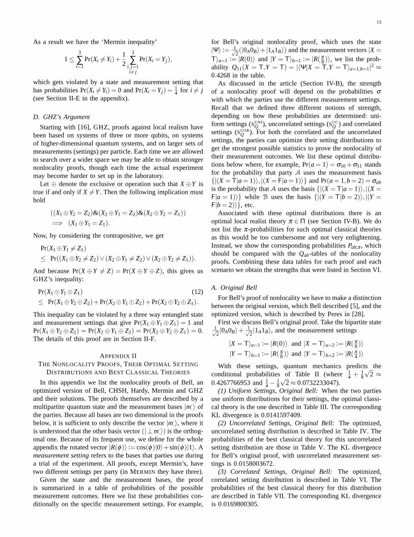
Starting with [16], GHZ, proofs against local realism havebeen based on systems of three or more qubits, on systemsof higher-dimensional quantum systems, and on larger sets ofmeasurements (settings) per particle. Each time we are allowedto search over a wider space we may be able to obtain strongernonlocality proofs, though each time the actual experimentmay become harder to set up in the laboratory.

Let ⊕ denote the exclusive or operation such thatX⊕Y istrue if and only ifX 6=Y. Then the following implication musthold

((X1⊕Y2 = Z2)&(X2⊕Y1 = Z2)&(X2⊕Y2 = Z1))=⇒ (X1⊕Y1 = Z1).

Now, by considering the contrapositive, we get

Pr(X1⊕Y1 6= Z1)≤ Pr((X1⊕Y2 6= Z2)∨ (X2⊕Y1 6= Z2)∨ (X2⊕Y2 6= Z1)).

And because Pr(X⊕Y 6= Z) = Pr(X⊕Y⊕Z), this gives usGHZ’s inequality:

Pr(X1⊕Y1⊕Z1) (12)

≤ Pr(X1⊕Y2⊕Z2)+Pr(X2⊕Y1⊕Z2)+Pr(X2⊕Y2⊕Z1).

This inequality can be violated by a three way entangled stateand measurement settings that give Pr(X1⊕Y1⊕Z1) = 1 andPr(X1⊕Y2⊕Z2) = Pr(X2⊕Y1⊕Z2) = Pr(X2⊕Y2⊕Z1) = 0.The details of this proof are in Section II-F.

APPENDIX IITHE NONLOCALITY PROOFS, THEIR OPTIMAL SETTING

DISTRIBUTIONS AND BEST CLASSICAL THEORIES

In this appendix we list the nonlocality proofs of Bell, anoptimized version of Bell, CHSH, Hardy, Mermin and GHZand their solutions. The proofs themselves are described by amultipartite quantum state and the measurement bases|m·

·〉 ofthe parties. Because all bases are two dimensional in the proofsbelow, it is sufficient to only describe the vector|m·

·〉, where itis understood that the other basis vector(| ⊥m·

·〉) is the orthog-onal one. Because of its frequent use, we define for the wholeappendix the rotated vector|R(φ)〉 := cos(φ)|0〉+sin(φ)|1〉. Ameasurement settingrefers to the bases that parties use duringa trial of the experiment. All proofs, except Mermin’s, havetwo different settings per party (in MERMIN they have three).

Given the state and the measurement bases, the proofis summarized in a table of probabilities of the possiblemeasurement outcomes. Here we list these probabilities con-ditionally on the specific measurement settings. For example,

for Bell’s original nonlocality proof, which uses the state|Ψ〉 := 1√

2(|0A0B〉+ |1A1B〉) and the measurement vectors|X =

T〉a=1 := |R(0)〉 and |Y = T〉b=1 := |R(π

8 )〉, we list the prob-ability Q11(X = T,Y = T) = |〈Ψ|X = T,Y = T〉a=1,b=1|2 ≈0.4268 in the table.

As discussed in the article (Section IV-B), the strengthof a nonlocality proof will depend on the probabilitiesσwith which the parties use the different measurement settings.Recall that we defined three different notions of strength,depending on how these probabilities are determined: uni-form settings (SUNI

Q ), uncorrelated settings (SUCQ ) and correlated

settings (SCORQ ). For both the correlated and the uncorrelated

settings, the parties can optimize their setting distributions toget the strongest possible statistics to prove the nonlocality oftheir measurement outcomes. We list these optimal distribu-tions below where, for example, Pr(a = 1) = σ10+σ11 standsfor the probability that partyA uses the measurement basis{|(X = T|a= 1)〉, |(X = F|a= 1)〉} and Pr(a= 1,b= 2) = σab

is the probability thatA uses the basis{|(X = T|a= 1)〉, |(X =F|a = 1)〉} while B uses the basis{|(Y = T|b = 2)〉, |(Y =F|b = 2)〉}, etc.

Associated with these optimal distributions there is anoptimal local realist theoryπ ∈ Π (see Section IV-B). We donot list theπ-probabilities for such optimal classical theoriesas this would be too cumbersome and not very enlightening.Instead, we show the corresponding probabilitiesPab;π , whichshould be compared with theQab-tables of the nonlocalityproofs. Combining these data tables for each proof and eachscenario we obtain the strengths that were listed in Section VI.

A. Original Bell

For Bell’s proof of nonlocality we have to make a distinctionbetween the original version, which Bell described [5], and theoptimized version, which is described by Peres in [28].

First we discuss Bell’s original proof. Take the bipartite state1√2|0A0B〉+ 1√

2|1A1B〉, and the measurement settings

|X = T〉a=1 := |R(0)〉 and |X = T〉a=2 := |R(π

8 )〉|Y = T〉b=1 := |R(π

8 )〉 and |Y = T〉b=2 := |R(π

4 )〉

With these settings, quantum mechanics predicts theconditional probabilities of Table II (where1

4 + 18

√2 ≈

0.4267766953 and14 −18

√2≈ 0.0732233047).

(1) Uniform Settings, Original Bell:When the two partiesuse uniform distributions for their settings, the optimal classi-cal theory is the one described in Table III. The correspondingKL divergence is 0.0141597409.

(2) Uncorrelated Settings, Original Bell:The optimized,uncorrelated setting distribution is described in Table IV. Theprobabilities of the best classical theory for this uncorrelatedsetting distribution are those in Table V. The KL divergencefor Bell’s original proof, with uncorrelated measurement set-tings is 0.0158003672.

(3) Correlated Settings, Original Bell:The optimized,correlated setting distribution is described in Table VI. Theprobabilities of the best classical theory for this distributionare described in Table VII. The corresponding KL divergenceis 0.0169800305.

14

TABLE II

QUANTUM PREDICTIONSORIGINAL BELL

a = 1 a = 2Qab(X = x,Y = y) x = T x = F x = T x = F

b = 1y = Ty = F

0.4267766953 0.07322330470.0732233047 0.4267766953

0.5 00 0.5

b = 2y = Ty = F

0.25 0.250.25 0.25

0.4267766953 0.07322330470.0732233047 0.4267766953

TABLE III

BEST CLASSICAL THEORY FORUNIFORM SETTINGS ORIGINAL BELL . KL D ISTANCE: 0.0141597409.

a = 1 a = 2Pab(X = x,Y = x) x = T x = F x = T x = F

b = 1y = Ty = F

0.3970311357 0.10296886430.1029688643 0.3970311357

0.5000000000 0.00000000000.0000000000 0.5000000000

b = 2y = Ty = F

0.2940622714 0.20593772860.2059377286 0.2940622714

0.3970311357 0.10296886430.1029688643 0.3970311357

TABLE IV

OPTIMIZED UNCORRELATEDSETTING DISTRIBUTION ORIGINAL BELL

Pr(A = a,B = b) = σab ∈ ΣUC a = 1 a = 2 Pr(B = b)b = 1 0.2316110419 0.1327830656 0.3643941076b = 2 0.4039948505 0.2316110419 0.6356058924

Pr(A = a) 0.6356058924 0.3643941076

TABLE V

BEST CLASSICAL THEORY FORUNCORRELATEDSETTINGS ORIGINAL BELL . KL D ISTANCE: 0.0158003672.

a = 1 a = 2Pab(X = x,Y = x) x = T x = F x = T x = F

b = 1y = Ty = F

0.3901023259 0.10989767410.1098976741 0.3901023259

0.5000000000 0.00000000000.0000000000 0.5000000000

b = 2y = Ty = F

0.2802046519 0.21979534810.2197953481 0.2802046519

0.3901023259 0.10989767410.1098976741 0.3901023259

TABLE VI

OPTIMIZED CORRELATED SETTING DISTRIBUTION ORIGINAL BELL

Pr(A = a,B = b) = σab ∈ Σ a = 1 a = 2

b = 1 0.2836084841 0.1020773549b = 2 0.3307056768 0.2836084841

TABLE VII

BEST CLASSICAL THEORY FORCORRELATED SETTINGS ORIGINAL BELL . KL D ISTANCE: 0.0169800305.

a = 1 a = 2Pab(X = x,Y = x) x = T x = F x = T x = F

b = 1y = Ty = F

0.3969913979 0.10300860210.1030086021 0.3969913979

0.4941498806 0.00585011940.0058501194 0.4941498806

b = 2y = Ty = F

0.2881326764 0.21186732360.2118673236 0.2881326764

0.3969913979 0.10300860210.1030086021 0.3969913979

15

B. Optimized Bell

Take the bipartite state1√2|0A0B〉+ 1√

2|1A1B〉, and the mea-

surement settings

|X = T〉a=1 := |R(0)〉 and |X = T〉a=2 := |R(π

6 )〉|Y = T〉b=1 := |R(0)〉 and |Y = T〉b=2 := |R(π

3 )〉.

With these settings, quantum mechanics predicts the condi-tional probabilities of Table VIII.

(1) Uniform Settings, Optimized Bell:For the uniformsetting distribution the best classical approximation is givenin Table IX, which gives a KL divergence of 0.0177632822.

(2) Uncorrelated Settings, Optimized Bell:The optimal,uncorrelated setting distribution is given in Table X. Theprobabilities of the best classical theory for this distributionare those of Table XI. The corresponding KL divergence is0.0191506613.

(3) Correlated Settings, Optimized Bell:The optimal cor-related setting distribution is given in Table XII. The prob-abilities of the best classical theory for this distribution isgiven in Table XIII. The corresponding KL divergence is0.0211293952.

C. CHSH

The bipartite state1√2|0A0B〉+ 1√

2|1A1B〉. A’s andB’s mea-

surement settings are:

|X = T〉a=1 := |R(0)〉 and |X = T〉a=2 := |R(π

4 )〉,|Y = T〉b=1 := |R(π

8 )〉 and |Y = T〉b=2 := |R(−π

8 )〉.

With these settings, quantum mechanics predicts the con-ditional probabilities of Table XIV (with 1

4 + 18

√2 ≈

0.4267766953 and14 −18

√2≈ 0.0732233047).

Uniform, Uncorrelated and Correlated Settings, CHSH:The optimal measurement settings is the uniform settings,where bothA and B use one of the two measurements withprobability 0.5 (that isσab = 0.25)

The optimal classical theory in this scenario has the prob-abilities of Table XV.

D. Hardy

The bipartite state α|0A0B〉 − β |1A1B〉, with α :=12

√2+2

√−13+6

√5 ≈ 0.907 and β :=

√1−α2 ≈ 0.421

(such that indeedα2 + β 2 = 1). A’s and B’s measurementsettings are now identical and given by:

|X = T〉a=1 = |Y = T〉b=1 :=√

β

α+β|0〉+

√α

α+β|1〉,

|X = T〉a=2 = |Y = T〉b=2 :=−√

β 3

α3+β 3 |0〉+√

α3

α3+β 3 |1〉.

With these settings, quantum mechanics predicts the condi-tional probabilities of Table XVI.

(1) Uniform Settings, Hardy:For uniform measurementsettings, the best classical theory to describe the quantum me-chanical statistics is given in Table XVII, with KL divergence:0.0278585182.

(2) Uncorrelated Settings, Hardy:The optimized uncorre-lated setting distribution is given in Table XVIII. The probabil-ities of the best classical theory for this distribution are in Ta-ble XIX. The corresponding KL divergence is 0.0279816333.

(3) Correlated Settings, Hardy:The optimized correlatedsetting distribution is given in Table XX. The probabilitiesof the best classical theory for this distribution are de-scribed in Table XXI. The corresponding KL divergence is0.0280347655.

E. Mermin

In [26], we find the following nonlocality proof with twoparties, three measurement settings, and two possible out-comes. Let the entangled state be1√

2(|0A0B〉+ |1A1B〉), and

the measurement settings:

|X = T〉a=1 = |Y = T〉b=1 := |0〉,|X = T〉a=2 = |Y = T〉b=2 := |R(2

3π)〉,|X = T〉a=3 = |Y = T〉b=3 := |R(4

3π)〉.

With these settings, quantum mechanics predicts the condi-tional probabilities of Table XXII.

(1) Uniform Settings, Mermin:The probabilities of the bestclassical theory for the uniform measurement settings is givein Table XXIII.

(2) Uncorrelated Settings, Mermin:The optimal uncorre-lated setting distribution is given in Table XXIV. The prob-abilities of the best classical theory for this distribution is inTable XXV.

(3) Correlated Settings, Mermin:The optimal correlatedsetting distribution is given in Table XXVI (note that thereare also other optimal distributions). The probabilities ofthe best classical theory for this specific distribution aredescribed in Table XXVII. The corresponding KL divergenceis 0.0211293952.

F. GHZ

The tripartite state1√2|0A0B0C〉+ 1√

2|1A1B1C〉. The settings

for all three parties are identical:

|X = T〉a=1 = |Y = T〉b=1 = |Z = T〉c=1 := 1√2|0〉+ 1√

2|1〉,

|X = T〉a=2 = |Y = T〉b=2 = |Z = T〉c=2 := 1√2|0〉+ i√

2|1〉.

With these settings, quantum mechanics predicts the condi-tional probabilities of Table XXVIII.

(1) Uniform and Uncorrelated Settings, GHZ:For all threesettings, the best possible classical statistics that approximatethe GHZ experiment is that of Table XXIX. The optimaluncorrelated setting is the uniform settings that samples alleight measurement settings with equal probability. The corre-sponding KL divergence is: 0.2075187496.

(2) Correlated Settings, GHZ:The optimal correlated set-ting samples with equal probability those four settings thatyield the (0.125,0) outcome probabilities (those are the set-tings where an even number of the measurements are measur-ing along them1 axis). The KL divergence in this setting istwice that of the previous uniform setting: 0.4150374993.

16

TABLE VIII

QUANTUM PREDICTIONSOPTIMIZED BELL

a = 1 a = 2Qab(X = x,Y = y) x = T x = F x = T x = F

b = 1y = Ty = F

0.5 00 0.5

0.375 0.1250.125 0.375

b = 2y = Ty = F

0.125 0.3750.375 0.125

0.375 0.1250.125 0.375

TABLE IX

BEST CLASSICAL THEORY FORUNIFORM SETTINGS OPTIMIZED BELL . KL D ISTANCE: 0.0177632822.

a = 1 a = 2Pab(X = x,Y = x) x = T x = F x = T x = F

b = 1y = Ty = F

0.5000000000 0.00000000000.0000000000 0.5000000000

0.3333333333 0.16666666670.1666666667 0.3333333333

b = 2y = Ty = F

0.1666666667 0.33333333330.3333333333 0.1666666667

0.3333333333 0.16666666670.1666666667 0.3333333333

TABLE X

OPTIMIZED UNCORRELATEDSETTING DISTRIBUTION OPTIMIZED BELL

Pr(A = a,B = b) = σab ∈ ΣUC a = 1 a = 2 Pr(B = b)b = 1 0.1497077788 0.2372131160 0.3869208948b = 2 0.2372131160 0.3758659893 0.6130791052

Pr(A = a) 0.3869208948 0.6130791052

TABLE XI

BEST CLASSICAL THEORY FORUNCORRELATEDSETTINGS OPTIMIZED BELL . KL D ISTANCE: 0.0191506613.

a = 1 a = 2Pab(X = x,Y = x) x = T x = F x = T x = F

b = 1y = Ty = F

0.5000000000 0.00000000000.0000000000 0.5000000000

0.3267978563 0.17320214360.1732021436 0.3267978563

b = 2y = Ty = F

0.1732021436 0.32679785630.3267978563 0.1732021436

0.3464042873 0.15359571270.1535957127 0.3464042873

TABLE XII

OPTIMIZED CORRELATED SETTING DISTRIBUTION OPTIMIZED BELL

Pr(A = a,B = b) = σab ∈ Σ a = 1 a = 2

b = 1 0.1046493146 0.2984502285b = 2 0.2984502285 0.2984502285

TABLE XIII

BEST CLASSICAL THEORY FORCORRELATED SETTINGS OPTIMIZED BELL . KL D ISTANCE: 0.0211293952.

a = 1 a = 2Pab(X = x,Y = x) x = T x = F x = T x = F

b = 1y = Ty = F

0.4927305107 0.00726948920.0072694892 0.4927305107

0.3357564964 0.16424350360.1642435036 0.3357564964

b = 2y = Ty = F

0.1642435036 0.33575649640.3357564964 0.1642435036

0.3357564964 0.16424350360.1642435036 0.3357564964

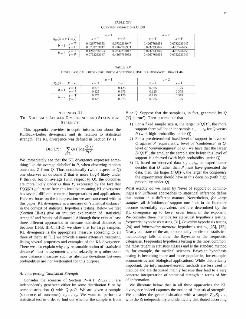
17

TABLE XIV

QUANTUM PREDICTIONSCHSH

a = 1 a = 2Qab(X = x,Y = y) x = T x = F x = T x = F

b = 1y = Ty = F

0.4267766953 0.07322330470.0732233047 0.4267766953

0.4267766953 0.07322330470.0732233047 0.4267766953

b = 2y = Ty = F

0.4267766953 0.07322330470.0732233047 0.4267766953

0.0732233047 0.42677669530.4267766953 0.0732233047

TABLE XV

BEST CLASSICAL THEORY FORUNIFORM SETTINGS CHSH. KL DISTANCE: 0.0462738469.

a = 1 a = 2Pab(X = x,Y = x) x = T x = F x = T x = F

b = 1y = Ty = F

0.375 0.1250.125 0.375

0.375 0.1250.125 0.375

b = 2y = Ty = F

0.375 0.1250.125 0.375

0.125 0.3750.375 0.125

APPENDIX IIITHE KULLBACK -LEIBLER DIVERGENCE AND STATISTICAL

STRENGTH

This appendix provides in-depth information about theKullback-Leiber divergence and its relation to statisticalstrength. The KL divergence was defined in Section IV as

D(Q‖P) := ∑z∈Z

Q(z) logQ(z)P(z)

.

We immediately see that the KL divergence expresses some-thing like the average disbelief inP, when observing randomoutcomesZ from Q. Thus occasionally (with respect toQ)one observes an outcomeZ that is more (log-) likely underP than Q, but on average (with respect toQ), the outcomesare more likely underQ than P, expressed by the fact thatD(Q‖P)≥ 0. Apart from this intuitive meaning, KL divergencehas several different concrete interpretations and applications.Here we focus on the interpretation we are concerned with inthis paper: KL divergence as a measure of ‘statistical distance’in the context of statistical hypothesis testing. Below we first(Section III-A) give an intuitive explanation of ‘statisticalstrength’ and ‘statistical distance’. Although there exist at leastthree different approaches to measure statistical distance, inSections III-B, III-C, III-D, we show that for large samples,KL divergence is the appropriate measure according to allthree of them. In [11] we provide a more extensive treatment,listing several properties and examples of the KL divergence.There we also explain why any reasonable notion of ‘statisticaldistance’ must be asymmetric, and, relatedly, why other com-mon distance measures such as absolute deviations betweenprobabilities arenot well-suited for this purpose.

A. Interpreting ‘Statistical Strength’

Consider the scenario of Section IV-A.1:Z1,Z2, . . . areindependently generated either by some distributionP or bysome distributionQ with Q 6= P. We are given a sample(sequence of outcomes)z1, . . . ,zn. We want to perform astatistical test in order to find out whether the sample is from

P or Q. Suppose that the sample is, in fact, generated byQ(‘Q is true’). Then it turns out that

1) For a fixed sample sizen, the largerD(Q‖P), the moresupport there will be in the samplez1, . . . ,zn for Q versusP (with high probability underQ) .

2) For a pre-determined fixed level of support in favor ofQ againstP (equivalently, level of ‘confidence’ inQ,level of ‘convincingness’ ofQ), we have that the largerD(Q‖P), the smaller the sample size before this level ofsupport is achieved (with high probability underQ).

3) If, based on observed dataz1, . . . ,zn, an experimenterdecides thatQ rather thanP must have generated thedata, then, the largerD(Q‖P), the larger theconfidencethe experimenter should have in this decision (with highprobability underQ).

What exactly do we mean by ‘level of support or convinc-ingness’? Different approaches to statistical inference definethis notion in a different manner. Nevertheless,for largesamples, all definitions of support one finds in the literaturebecome essentially equivalent, and are determined by theKL divergence up to lower order terms in the exponent.We consider three methods for statistical hypothesis testing:frequentisthypothesis testing [31],Bayesianhypothesis testing[24] and information-theoretichypothesis testing [25], [32].Nearly all state-of-the-art, theoretically motivated statisticalmethodology falls in either the Bayesian or the frequentistcategories. Frequentist hypothesis testing is the most common,the most taught in statistics classes and is the standard methodin, for example, the medical sciences. Bayesian hypothesistesting is becoming more and more popular in, for example,econometrics and biological applications. While theoreticallyimportant, the information-theoretic methods are less used inpractice and are discussed mainly because they lead to a veryconcrete interpretation of statistical strength in terms ofbitsof information.

We illustrate below that in all three approaches the KLdivergence indeed captures the notion of ‘statistical strength’.We consider the general situation with a sampleZ1,Z2, . . . ,with theZi independently and identically distributed according

18

TABLE XVI

QUANTUM PREDICTIONSHARDY

a = 1 a = 2Qab(X = x,Y = y) x = T x = F x = T x = F

b = 1y = Ty = F

0 0.381966011250.38196601125 0.23606797750

0.23606797750 0.145898033750 0.61803398875

b = 2y = Ty = F

0.23606797750 00.14589803375 0.61803398875

0.09016994375 0.145898033750.14589803375 0.61803398875

TABLE XVII

BEST CLASSICAL THEORY FORUNIFORM SETTINGS HARDY. KL D ISTANCE: 0.0278585182.

a = 1 a = 2Pab(X = x,Y = x) x = T x = F x = T x = F

b = 1y = Ty = F

0.0338829434 0.35436403630.3543640363 0.2573889840

0.2190090188 0.16923796090.0075052045 0.6042478158

b = 2y = Ty = F

0.2190090188 0.00750520450.1692379609 0.6042478158

0.0488933524 0.17762087090.1776208709 0.5958649058

TABLE XVIII

OPTIMIZED UNCORRELATEDSETTING DISTRIBUTION HARDY

Pr(A = a,B = b) = σab ∈ ΣUC a = 1 a = 2 Pr(B = b)b = 1 0.2603092699 0.2498958554 0.5102051253b = 2 0.2498958554 0.2398990193 0.4897948747

Pr(A = a) 0.5102051253 0.4897948747

TABLE XIX

BEST CLASSICAL THEORY FORUNCORRELATEDSETTINGS HARDY. KL D ISTANCE: 0.0279816333.

a = 1 a = 2Pab(X = x,Y = x) x = T x = F x = T x = F

b = 1y = Ty = F

0.0198831449 0.36122137690.3612213769 0.2576741013

0.2143180373 0.16678648440.0141212511 0.6047742271

b = 2y = Ty = F

0.2143180373 0.01412125110.1667864844 0.6047742271

0.0481256471 0.18031364140.1803136414 0.5912470702

TABLE XX

OPTIMIZED CORRELATED SETTING DISTRIBUTION HARDY

Pr(A = a,B = b) = σab ∈ Σ a = 1 a = 2

b = 1 0.2562288294 0.2431695652b = 2 0.2431695652 0.2574320402

TABLE XXI

BEST CLASSICAL THEORY FORCORRELATED SETTINGS HARDY. KL D ISTANCE: 0.0280347655.

a = 1 a = 2Pab(X = x,Y = x) x = T x = F x = T x = F

b = 1y = Ty = F

0.0173443545 0.36203766080.3620376608 0.2585803238

0.2123471649 0.16703485040.0165954828 0.6040225019

b = 2y = Ty = F

0.2123471649 0.01659548280.1670348504 0.6040225019

0.0505353201 0.17840732760.1784073276 0.5926500247

19

TABLE XXII

QUANTUM PREDICTIONSMERMIN

a = 1 a = 2 a = 3Qab(X = x,Y = y) x = T x = F x = T x = F x = T x = F

b = 1y = Ty = F

0.5 00 0.5

0.125 0.3750.375 0.125

0.125 0.3750.375 0.125

b = 2y = Ty = F

0.125 0.3750.375 0.125

0.5 00 0.5

0.125 0.3750.375 0.125

b = 3y = Ty = F

0.125 0.3750.375 0.125

0.125 0.3750.375 0.125

0.5 00 0.5

TABLE XXIII

BEST CLASSICAL THEORY FORUNIFORM SETTINGS MERMIN. KL DIVERGENCE: 0.0157895843.

a = 1 a = 2 a = 3Pab(X = x,Y = y) x = T x = F x = T x = F x = T x = F

b = 1y = Ty = F

0.50000 0.000000.00000 0.50000

0.16667 0.333330.33333 0.16667

0.16667 0.333330.33333 0.16667

b = 2y = Ty = F

0.16667 0.333330.33333 0.16667

0.50000 0.000000.00000 0.50000

0.16667 0.333330.33333 0.16667

b = 3y = Ty = F

0.16667 0.333330.33333 0.16667

0.16667 0.333330.33333 0.16667

0.50000 0.000000.00000 0.50000

TABLE XXIV

OPTIMIZED UNCORRELATEDSETTING DISTRIBUTION MERMIN

σab ∈ ΣUC a = 1 a = 2 a = 3 Pr(B = b)b = 1 0.1497077711 0 0.2372131137 0.3869208848b = 2 0.2372131137 0 0.3758660015 0.6130791152b = 3 0 0 0 0

Pr(A = a) 0.3869208848 0 0.6130791152

TABLE XXV

BEST CLASSICAL THEORY FORUNCORRELATEDSETTINGS MERMIN. KL D ISTANCE: 0.0191506613.

a = 1 a = 2 a = 3Pab(X = x,Y = y) x = T x = F x = T x = F x = T x = F

b = 1y = Ty = F

0.50000 0.000000.00000 0.50000

0.50000 0.000000.50000 0.00000

0.17320 0.326800.32680 0.17320

b = 2y = Ty = F

0.17320 0.326800.32680 0.17320

0.50000 0.000000.50000 0.00000

0.15360 0.346400.34640 0.15360

b = 3y = Ty = F

0.50000 0.500000.00000 0.00000

1.00000 0.000000.00000 0.00000

0.50000 0.500000.00000 0.00000

TABLE XXVI

OPTIMIZED CORRELATED SETTING DISTRIBUTION MERMIN

Pr(A = a,B = b) = σab ∈ Σ a = 1 a = 2 a = 3

b = 1 0.1046493071 0 0.2984502310b = 2 0.2984502310 0 0.2984502310b = 3 0 0 0

TABLE XXVII

BEST CLASSICAL THEORY FORCORRELATED SETTINGS MERMIN. KL D ISTANCE: 0.0211293952.

a = 1 a = 2 a = 3Pab(X = x,Y = y) x = T x = F x = T x = F x = T x = F

b = 1y = Ty = F

0.49273 0.007270.00727 0.49273

0.50000 0.000000.50000 0.00000

0.16424 0.335760.33576 0.16424

b = 2y = Ty = F

0.16424 0.335760.33576 0.16424

0.50000 0.000000.50000 0.00000

0.16424 0.335760.33576 0.16424

b = 3y = Ty = F

0.50000 0.500000.00000 0.00000

1.00000 0.000000.00000 0.00000

0.50000 0.500000.00000 0.00000

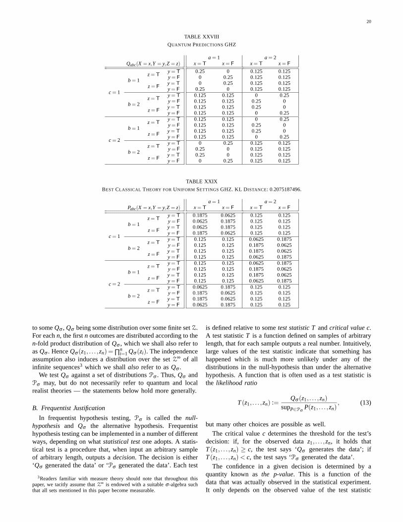
20

TABLE XXVIII

QUANTUM PREDICTIONSGHZ

a = 1 a = 2Qabc(X = x,Y = y,Z = z) x = T x = F x = T x = F

c = 1

b = 1z= T

y = Ty = F

z= Fy = Ty = F

b = 2z= T

y = Ty = F

z= Fy = Ty = F

0.25 00 0.250 0.25

0.25 00.125 0.1250.125 0.1250.125 0.1250.125 0.125

0.125 0.1250.125 0.1250.125 0.1250.125 0.125

0 0.250.25 00.25 0

0 0.25

c = 2

b = 1z= T

y = Ty = F

z= Fy = Ty = F

b = 2z= T

y = Ty = F

z= Fy = Ty = F

0.125 0.1250.125 0.1250.125 0.1250.125 0.125

0 0.250.25 00.25 0

0 0.25

0 0.250.25 00.25 0

0 0.250.125 0.1250.125 0.1250.125 0.1250.125 0.125

TABLE XXIX

BEST CLASSICAL THEORY FORUNIFORM SETTINGS GHZ. KL D ISTANCE: 0.2075187496.

a = 1 a = 2Pabc(X = x,Y = y,Z = z) x = T x = F x = T x = F

c = 1

b = 1z= T

y = Ty = F

z= Fy = Ty = F

b = 2z= T

y = Ty = F

z= Fy = Ty = F

0.1875 0.06250.0625 0.18750.0625 0.18750.1875 0.06250.125 0.1250.125 0.1250.125 0.1250.125 0.125

0.125 0.1250.125 0.1250.125 0.1250.125 0.1250.0625 0.18750.1875 0.06250.1875 0.06250.0625 0.1875

c = 2

b = 1z= T

y = Ty = F

z= Fy = Ty = F

b = 2z= T

y = Ty = F

z= Fy = Ty = F

0.125 0.1250.125 0.1250.125 0.1250.125 0.1250.0625 0.18750.1875 0.06250.1875 0.06250.0625 0.1875

0.0625 0.18750.1875 0.06250.1875 0.06250.0625 0.18750.125 0.1250.125 0.1250.125 0.1250.125 0.125

to someQσ , Qσ being some distribution over some finite setZ.For eachn, the firstn outcomes are distributed according to then-fold product distribution ofQσ , which we shall also refer toasQσ . HenceQσ (z1, . . . ,zn) = ∏n

i=1Qσ (zi). The independenceassumption also induces a distribution over the setZ∞ of allinfinite sequences3 which we shallalso refer to asQσ .

We testQσ against a set of distributionsPσ . Thus,Qσ andPσ may, but do not necessarily refer to quantum and localrealist theories — the statements below hold more generally.

B. Frequentist Justification

In frequentist hypothesis testing,Pσ is called thenull-hypothesisand Qσ the alternative hypothesis. Frequentisthypothesis testing can be implemented in a number of differentways, depending on whatstatistical testone adopts. A statis-tical test is a procedure that, when input an arbitrary sampleof arbitrary length, outputs adecision. The decision is either‘Qσ generated the data’ or ‘Pσ generated the data’. Each test

3Readers familiar with measure theory should note that throughout thispaper, we tacitly assume thatZ∞ is endowed with a suitableσ -algebra suchthat all sets mentioned in this paper become measurable.

is defined relative to sometest statistic Tandcritical value c.A test statisticT is a function defined on samples of arbitrarylength, that for each sample outputs a real number. Intuitively,large values of the test statistic indicate that something hashappened which is much more unlikely under any of thedistributions in the null-hypothesis than under the alternativehypothesis. A function that is often used as a test statistic isthe likelihood ratio

T(z1, . . . ,zn) :=Qσ (z1, . . . ,zn)

supP∈PσP(z1, . . . ,zn)

, (13)

but many other choices are possible as well.

The critical valuec determines the threshold for the test’sdecision: if, for the observed dataz1, . . . ,zn, it holds thatT(z1, . . . ,zn) ≥ c, the test says ‘Qσ generates the data’; ifT(z1, . . . ,zn) < c, the test says ‘Pσ generated the data’.

The confidence in a given decision is determined by aquantity known asthe p-value. This is a function of thedata that was actually observed in the statistical experiment.It only depends on the observed value of the test statistic

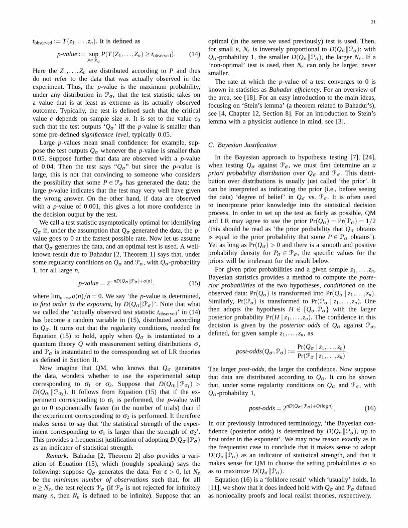
21

tobserved:= T(z1, . . . ,zn). It is defined as

p-value:= supP∈Pσ

P(T(Z1, . . . ,Zn)≥ tobserved). (14)

Here theZ1, . . . ,Zn are distributed according toP and thusdo not refer to the data that was actually observed in theexperiment. Thus, thep-value is the maximum probability,under any distribution inPσ , that the test statistic takes ona value that is at least as extreme as its actually observedoutcome. Typically, the test is defined such that the criticalvalue c depends on sample sizen. It is set to the valuec0

such that the test outputs ‘Qσ ’ iff the p-value is smaller thansome pre-definedsignificance level, typically 0.05.

Large p-values mean small confidence: for example, sup-pose the test outputsQσ whenever thep-value is smaller than0.05. Suppose further that data are observed with ap-valueof 0.04. Then the test says “Qσ ” but since thep-value islarge, this is not that convincing to someone who considersthe possibility that someP∈ Pσ has generated the data: thelarge p-value indicates that the test may very well have giventhe wrong answer. On the other hand, if data are observedwith a p-value of 0.001, this gives a lot more confidence inthe decision output by the test.

We call a test statistic asymptotically optimal for identifyingQσ if, under the assumption thatQσ generated the data, thep-value goes to 0 at the fastest possible rate. Now let us assumethatQσ generates the data, and an optimal test is used. A well-known result due to Bahadur [2, Theorem 1] says that, undersome regularity conditions onQσ andPσ , with Qσ -probability1, for all largen,

p-value= 2−nD(Qσ ‖Pσ )+o(n). (15)

where limn→∞ o(n)/n= 0. We say ‘thep-value is determined,to first order in the exponent, by D(Qσ‖Pσ )’. Note that whatwe called the ‘actually observed test statistictobserved’ in (14)has become a random variable in (15), distributed accordingto Qσ . It turns out that the regularity conditions, needed forEquation (15) to hold, apply whenQσ is instantiated to aquantum theoryQ with measurement setting distributionsσ ,andPσ is instantiated to the corresponding set of LR theoriesas defined in Section II.

Now imagine that QM, who knows thatQσ generatesthe data, wonders whether to use the experimental setupcorresponding toσ1 or σ2. Suppose thatD(Qσ1‖Pσ1) >D(Qσ1‖Pσ2). It follows from Equation (15) that if the ex-periment corresponding toσ1 is performed, thep-value willgo to 0 exponentially faster (in the number of trials) than ifthe experiment corresponding toσ2 is performed. It thereforemakes sense to say that ‘the statistical strength of the exper-iment corresponding toσ1 is larger than the strength ofσ2’.This provides a frequentist justification of adoptingD(Qσ‖Pσ )as an indicator of statistical strength.

Remark: Bahadur [2, Theorem 2] also provides a vari-ation of Equation (15), which (roughly speaking) says thefollowing: supposeQσ generates the data. Forε > 0, let Nε

be the minimum number of observationssuch that, for alln≥Nε , the test rejectsPσ (if Pσ is not rejected for infinitelymany n, then Nε is defined to be infinite). Suppose that an

optimal (in the sense we used previously) test is used. Then,for small ε, Nε is inversely proportional toD(Qσ‖Pσ ): withQσ -probability 1, the smallerD(Qσ‖Pσ ), the largerNε . If a‘non-optimal’ test is used, thenNε can only be larger, neversmaller.

The rate at which thep-value of a test converges to 0 isknown in statistics asBahadur efficiency. For an overview ofthe area, see [18]. For an easy introduction to the main ideas,focusing on ‘Stein’s lemma’ (a theorem related to Bahadur’s),see [4, Chapter 12, Section 8]. For an introduction to Stein’slemma with a physicist audience in mind, see [3].

C. Bayesian Justification

In the Bayesian approach to hypothesis testing [7], [24],when testingQσ againstPσ , we must first determine anapriori probability distribution over Qσ and Pσ . This distri-bution over distributions is usually just called ‘the prior’. Itcan be interpreted as indicating the prior (i.e., before seeingthe data) ‘degree of belief’ inQσ vs. Pσ . It is often usedto incorporate prior knowledge into the statistical decisionprocess. In order to set up the test as fairly as possible, QMand LR may agree to use the prior Pr(Qσ ) = Pr(Pσ ) = 1/2(this should be read as ‘the prior probability thatQσ obtainsis equal to the prior probability that someP∈ Pσ obtains’).Yet as long as Pr(Qσ ) > 0 and there is a smooth and positiveprobability density forPσ ∈ Pσ , the specific values for thepriors will be irrelevant for the result below.

For given prior probabilities and a given samplez1, . . . ,zn,Bayesian statistics provides a method to compute theposte-rior probabilities of the two hypotheses,conditionedon theobserved data: Pr(Qσ ) is transformed into Pr(Qσ | z1, . . . ,zn).Similarly, Pr(Pσ ) is transformed to Pr(Pσ | z1, . . . ,zn). Onethen adopts the hypothesisH ∈ {Qσ ,Pσ} with the largerposterior probability Pr(H | z1, . . . ,zn). The confidence in thisdecision is given by theposterior oddsof Qσ againstPσ ,defined, for given samplez1, . . . ,zn, as

post-odds(Qσ ,Pσ ) :=Pr(Qσ | z1, . . . ,zn)Pr(Pσ | z1, . . . ,zn)

.

The largerpost-odds, the larger the confidence. Now supposethat data are distributed according toQσ . It can be shownthat, under some regularity conditions onQσ and Pσ , withQσ -probability 1,

post-odds= 2nD(Qσ ‖Pσ )+O(logn), (16)

In our previously introduced terminology, ‘the Bayesian con-fidence (posterior odds) is determined byD(Qσ‖Pσ ), up tofirst order in the exponent’. We may now reason exactly as inthe frequentist case to conclude that it makes sense to adoptD(Qσ‖Pσ ) as an indicator of statistical strength, and that itmakes sense for QM to choose the setting probabilitiesσ soas to maximizeD(Qσ‖Pσ ).

Equation (16) is a ‘folklore result’ which ‘usually’ holds. In[11], we show that it does indeed hold withQσ andPσ definedas nonlocality proofs and local realist theories, respectively.

22

D. Information-Theoretic Justification

There exist several approaches to information-theoretic orcompression-based hypothesis testing; see, for example, [4],[25]. The most influential of these is the so-calledMinimumDescription Length Principle[32]. The basic idea is alwaysthat the more one can compress a given sequence of data, themore regularity one has extracted from the data, and thus, thebetter one has captured the ‘underlying regularities in the data’.Thus, the hypothesis that allows for the maximum compressionof the data should be adopted.

Let us first consider testing a simple hypothesisQ againstanother simple hypothesisP. Two basic facts of coding theorysay that

1) There exists a uniquely decodable code with lengthsLQ

that satisfy, for allz1, . . . ,zn ∈ Zn,

LQ(z1, . . . ,zn) = d− logQ(z1, . . . ,zn)e.

The code with lengthsLQ is called theShannon-Fanocode, and its existence follows from the so-calledKraftInequality, [10].

2) If data Z1, . . . ,Zn are independently identically dis-tributed∼Q, then among all uniquely decodable codes,the code with length functionLQ has the shortest ex-pected code-length. That is, letL be the length functionof any uniquely decodable code overn outcomes, then

EQ[L(Z1, . . . ,Zn)]≥ EQ[− logQ(Z1, . . . ,Zn)].

Thus, under the assumption thatQ generated the data, theoptimal (maximally compressing) code to use will be theShannon-Fano code with lengths− logQ(Zn) (here, as in theremainder of this section, we ignored the integer requirementfor code lengths). Similarly, under the assumption that someP with P 6= Q generated the data the optimal code will be thecode with lengths− logP(Zn). Thus, from the information-theoretic point of view, if one wants to find out whetherPor Q better explains the data, one should check whether theoptimal code underP or the optimal code underQ allows formore compression of the data. That is, one should look at thedifference

bit-diff :=− logP(z1, . . . ,zn)− [− logQ(z1, . . . ,zn)]. (17)

If bit-diff > 0, then one decides thatQ better explains the data.The confidence in this decision is given by the magnitude ofbit-diff: the largerbit-diff, the more extra bits one needs toencode the data underP rather thanQ, thus the larger theconfidence inQ.

Now suppose thatQ actually generates the data. Theexpected code length difference, measured in bits, betweencoding the data using the optimal code forQ and codingusing the optimal code forP, is given byEQ[− logP(Zn)−[− logQ(Zn)]] = nD(Q‖P). Thus, the KL divergence can beinterpreted asthe expected additional number of bits neededto encode outcomes generated by Q, if outcomes are encodedusing a code that is optimal for P rather than for Q. Thus,the natural ‘unit’ ofD(·‖·) is the ‘bit’, andD(Q‖P) may beviewed as ‘average amount of information aboutZ that is lostif Z is wrongfully regarded as being distributed byQ rather

than P’. By the law of large numbers, Equation (17) impliesthat, with Q-probability 1, asn→ ∞,

1n(bit-diff)→ D(Q‖P). (18)

Thus, if Q generates the data, then the information-theoreticconfidencebit-diff in decision “Q explains the data better thanP” is, up to first order, determined by the KL divergencebetweenQ andP: the largerD(Q‖P), the larger the confidence.This gives an information-theoretic justification of the useof the KL divergence as an indicator of statistical strengthfor simple hypothesis testing. We now turn to compositehypothesis testing.

Composite Hypothesis Testing:If one comparesQσ

against a set of hypothesesPσ , then one has to associatePσ

with a code that is ‘optimal under the assumption that someP∈ Pσ generated the data’. It turns out that there exist codeswith lengthsLP satisfying, for allz1, . . . ,zn ∈ Zn,

LPσ(z1, . . . ,zn)≤ inf

P∈Pσ

− logP(z1, . . . ,zn)+O(logn).

An example of such a code is given in [11]. The codeLPσ

is optimal, up to logarithmic terms, for whatever distributionP ∈ Pσ that might actually generate data. The informationtheoretic approach to hypothesis testing now tells us that, totestQσ againstPσ , we should compute the difference in codelengths

bit-diff := LPσ(z1, . . . ,zn)− [− logQσ (z1, . . . ,zn)].

The larger this difference, the larger the confidence thatQσ

rather thanPσ generated the data. The article [11] shows that,in analogy to Equation (18), asn→ ∞,

1n(bit-diff)→ D(Qσ‖Pσ ) (19)

Thus, up to sublinear terms, the information-theoretic con-fidence in Qσ is given by nD(Qσ‖Pσ ). This provides aninformation-theoretic justification of adoptingD(Qσ‖Pσ ) asan indicator of statistical strength.

APPENDIX IVPROOFS OFTHEOREMS1,2 AND 3

A. Preparation

The proof of Theorem 1 uses the following lemma, whichis of some independent interest.

Lemma 1:Let (Σ,Π,U) be the game corresponding to anarbitrary 2 party, 2 measurement settings per party nonlocalityproof. For any(a0,b0)∈ {1,2}2, there exists aπ ∈Π such thatfor all (a,b) ∈ {1,2}2\{(a0,b0)} we haveQab = Pab;π . Thus,for any three of the four measurement settings, the probabilitydistribution on outcomes can be perfectly explained by a localrealist theory.

Proof: We give a detailed proof for the case that themeasurement outcomes are two values{T,F}; the general casecan be proved in a similar way.

Without loss of generality let(a0,b0) = (2,2). Now we mustprove that the equationQab = Pab;π holds for the three settings(a,b)∈{(1,1),(1,2),(2,1)}. Every triple of distributionsPab;π

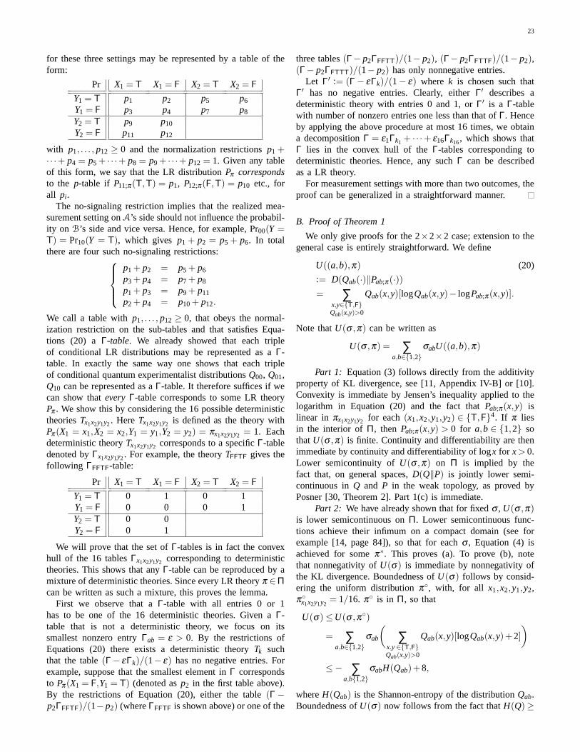
23

for these three settings may be represented by a table of theform:

Pr X1 = T X1 = F X2 = T X2 = F

Y1 = T p1 p2 p5 p6

Y1 = F p3 p4 p7 p8

Y2 = T p9 p10

Y2 = F p11 p12

with p1, . . . , p12 ≥ 0 and the normalization restrictionsp1 +· · ·+ p4 = p5 + · · ·+ p8 = p9 + · · ·+ p12 = 1. Given any tableof this form, we say that the LR distributionPπ correspondsto the p-table if P11;π(T,T) = p1, P12;π(F,T) = p10 etc., forall pi .

The no-signaling restriction implies that the realized mea-surement setting onA’s side should not influence the probabil-ity on B’s side and vice versa. Hence, for example, Pr00(Y =T) = Pr10(Y = T), which gives p1 + p2 = p5 + p6. In totalthere are four such no-signaling restrictions:

p1 + p2 = p5 + p6

p3 + p4 = p7 + p8

p1 + p3 = p9 + p11

p2 + p4 = p10+ p12.

We call a table withp1, . . . , p12 ≥ 0, that obeys the normal-ization restriction on the sub-tables and that satisfies Equa-tions (20) a Γ-table. We already showed that each tripleof conditional LR distributions may be represented as aΓ-table. In exactly the same way one shows that each tripleof conditional quantum experimentalist distributionsQ00, Q01,Q10 can be represented as aΓ-table. It therefore suffices if wecan show thateveryΓ-table corresponds to some LR theoryPπ . We show this by considering the 16 possible deterministictheoriesTx1x2y1y2. HereTx1x2y1y2 is defined as the theory withPπ(X1 = x1,X2 = x2,Y1 = y1,Y2 = y2) = πx1x2y1y2 = 1. Eachdeterministic theoryTx1x2y1y2 corresponds to a specificΓ-tabledenoted byΓx1x2y1y2. For example, the theoryTFFTF gives thefollowing ΓFFTF-table:

Pr X1 = T X1 = F X2 = T X2 = F

Y1 = T 0 1 0 1Y1 = F 0 0 0 1Y2 = T 0 0Y2 = F 0 1

We will prove that the set ofΓ-tables is in fact the convexhull of the 16 tablesΓx1x2y1y2 corresponding to deterministictheories. This shows that anyΓ-table can be reproduced by amixture of deterministic theories. Since every LR theoryπ ∈Πcan be written as such a mixture, this proves the lemma.

First we observe that aΓ-table with all entries 0 or 1has to be one of the 16 deterministic theories. Given aΓ-table that is not a deterministic theory, we focus on itssmallest nonzero entryΓab = ε > 0. By the restrictions ofEquations (20) there exists a deterministic theoryTk suchthat the table(Γ− εΓk)/(1− ε) has no negative entries. Forexample, suppose that the smallest element inΓ correspondsto Pπ(X1 = F,Y1 = T) (denoted asp2 in the first table above).By the restrictions of Equation (20), either the table(Γ−p2ΓFFTF)/(1−p2) (whereΓFFTF is shown above) or one of the

three tables(Γ− p2ΓFFTT)/(1− p2), (Γ− p2ΓFTTF)/(1− p2),(Γ− p2ΓFTTT)/(1− p2) has only nonnegative entries.

Let Γ′ := (Γ− εΓk)/(1− ε) where k is chosen such thatΓ′ has no negative entries. Clearly, eitherΓ′ describes adeterministic theory with entries 0 and 1, orΓ′ is a Γ-tablewith number of nonzero entries one less than that ofΓ. Henceby applying the above procedure at most 16 times, we obtaina decompositionΓ = ε1Γk1 + · · ·+ ε16Γk16, which shows thatΓ lies in the convex hull of theΓ-tables corresponding todeterministic theories. Hence, any suchΓ can be describedas a LR theory.

For measurement settings with more than two outcomes, theproof can be generalized in a straightforward manner.

B. Proof of Theorem 1

We only give proofs for the 2×2×2 case; extension to thegeneral case is entirely straightforward. We define

U((a,b),π) (20)

:= D(Qab(·)‖Pab;π(·))= ∑

x,y∈{T,F}Qab(x,y)>0

Qab(x,y)[logQab(x,y)− logPab;π(x,y)].

Note thatU(σ ,π) can be written as

U(σ ,π) = ∑a,b∈{1,2}

σabU((a,b),π)

Part 1: Equation (3) follows directly from the additivityproperty of KL divergence, see [11, Appendix IV-B] or [10].Convexity is immediate by Jensen’s inequality applied to thelogarithm in Equation (20) and the fact thatPab;π(x,y) islinear in πx1x2y1y2 for each(x1,x2,y1,y2) ∈ {T,F}4. If π liesin the interior of Π, then Pab;π(x,y) > 0 for a,b ∈ {1,2} sothatU(σ ,π) is finite. Continuity and differentiability are thenimmediate by continuity and differentiability of logx for x> 0.Lower semicontinuity ofU(σ ,π) on Π is implied by thefact that, on general spaces,D(Q‖P) is jointly lower semi-continuous inQ and P in the weak topology, as proved byPosner [30, Theorem 2]. Part 1(c) is immediate.

Part 2: We have already shown that for fixedσ , U(σ ,π)is lower semicontinuous onΠ. Lower semicontinuous func-tions achieve their infimum on a compact domain (see forexample [14, page 84]), so that for eachσ , Equation (4) isachieved for someπ∗. This proves (a). To prove (b), notethat nonnegativity ofU(σ) is immediate by nonnegativity ofthe KL divergence. Boundedness ofU(σ) follows by consid-ering the uniform distributionπ◦, with, for all x1,x2,y1,y2,π◦x1x2y1y2

= 1/16. π◦ is in Π, so that

U(σ)≤U(σ ,π◦)

= ∑a,b∈{1,2}

σab

(∑

x,y∈{T,F}Qab(x,y)>0

Qab(x,y)[logQab(x,y)+2])

≤− ∑a,b{1,2}

σabH(Qab)+8,

whereH(Qab) is the Shannon-entropy of the distributionQab.Boundedness ofU(σ) now follows from the fact thatH(Q)≥

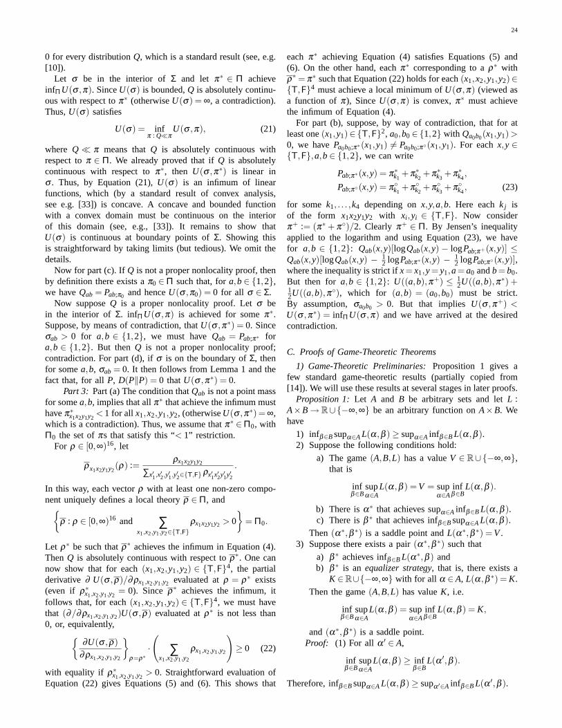
24

0 for every distributionQ, which is a standard result (see, e.g.[10]).

Let σ be in the interior ofΣ and let π∗ ∈ Π achieveinfΠU(σ ,π). SinceU(σ) is bounded,Q is absolutely continu-ous with respect toπ∗ (otherwiseU(σ) = ∞, a contradiction).Thus,U(σ) satisfies

U(σ) = infπ : Q�π

U(σ ,π), (21)

where Q � π means thatQ is absolutely continuous withrespect toπ ∈ Π. We already proved that ifQ is absolutelycontinuous with respect toπ∗, then U(σ ,π∗) is linear inσ . Thus, by Equation (21),U(σ) is an infimum of linearfunctions, which (by a standard result of convex analysis,see e.g. [33]) is concave. A concave and bounded functionwith a convex domain must be continuous on the interiorof this domain (see, e.g., [33]). It remains to show thatU(σ) is continuous at boundary points ofΣ. Showing thisis straightforward by taking limits (but tedious). We omit thedetails.

Now for part (c). IfQ is not a proper nonlocality proof, thenby definition there exists aπ0 ∈Π such that, fora,b∈ {1,2},we haveQab = Pab;π0 and henceU(σ ,π0) = 0 for all σ ∈ Σ.

Now supposeQ is a proper nonlocality proof. Letσ bein the interior of Σ. infΠU(σ ,π) is achieved for someπ∗.Suppose, by means of contradiction, thatU(σ ,π∗) = 0. Sinceσab > 0 for a,b ∈ {1,2}, we must haveQab = Pab;π∗ fora,b ∈ {1,2}. But then Q is not a proper nonlocality proof;contradiction. For part (d), ifσ is on the boundary ofΣ, thenfor somea,b, σab = 0. It then follows from Lemma 1 and thefact that, for allP, D(P‖P) = 0 thatU(σ ,π∗) = 0.

Part 3: Part (a) The condition thatQab is not a point massfor somea,b, implies that allπ∗ that achieve the infimum musthaveπ∗x1x2y1y2

< 1 for all x1,x2,y1,y2, (otherwiseU(σ ,π∗) = ∞,which is a contradiction). Thus, we assume thatπ∗ ∈Π0, withΠ0 the set ofπs that satisfy this “< 1” restriction.

For ρ ∈ [0,∞)16, let

ρx1x2y1y2(ρ) :=

ρx1x2y1y2

∑x′1,x′2,y′1,y′2∈{T,F}ρx′1x′2y′1y′2

.

In this way, each vectorρ with at least one non-zero compo-nent uniquely defines a local theoryρ ∈ Π, and{

ρ : ρ ∈ [0,∞)16 and ∑x1,x2,y1,y2∈{T,F}

ρx1x2y1y2 > 0

}= Π0.

Let ρ∗ be such thatρ∗ achieves the infimum in Equation (4).ThenQ is absolutely continuous with respect toρ

∗. One cannow show that for each(x1,x2,y1,y2) ∈ {T,F}4, the partialderivative ∂ U(σ ,ρ)/∂ρx1,x2,y1,y2 evaluated atρ = ρ∗ exists(even if ρ∗x1,x2,y1,y2

= 0). Sinceρ∗ achieves the infimum, it

follows that, for each(x1,x2,y1,y2) ∈ {T,F}4, we must havethat (∂/∂ρx1,x2,y1,y2)U(σ ,ρ) evaluated atρ∗ is not less than0, or, equivalently,{

∂U(σ ,ρ)∂ρx1,x2,y1,y2

}ρ=ρ∗

·

(∑

x1,x2,y1,y2

ρx1,x2,y1,y2

)≥ 0 (22)

with equality if ρ∗x1,x2,y1,y2> 0. Straightforward evaluation of

Equation (22) gives Equations (5) and (6). This shows that

each π∗ achieving Equation (4) satisfies Equations (5) and(6). On the other hand, eachπ∗ corresponding to aρ∗ withρ∗ = π∗ such that Equation (22) holds for each(x1,x2,y1,y2)∈

{T,F}4 must achieve a local minimum ofU(σ ,π) (viewed asa function ofπ), SinceU(σ ,π) is convex,π∗ must achievethe infimum of Equation (4).

For part (b), suppose, by way of contradiction, that for atleast one(x1,y1)∈{T,F}2, a0,b0∈{1,2} with Qa0b0(x1,y1) >0, we havePa0b0;π∗(x1,y1) 6= Pa0b0;π◦(x1,y1). For eachx,y ∈{T,F},a,b∈ {1,2}, we can write

Pab;π∗(x,y) = π∗k1

+π∗k2

+π∗k3

+π∗k4

,

Pab;π◦(x,y) = π◦k1

+π◦k2

+π◦k3

+π◦k4

, (23)

for some k1, . . . ,k4 depending onx,y,a,b. Here eachk j isof the form x1x2y1y2 with xi ,yi ∈ {T,F}. Now considerπ+ := (π∗ + π◦)/2. Clearly π+ ∈ Π. By Jensen’s inequalityapplied to the logarithm and using Equation (23), we havefor a,b ∈ {1,2}: Qab(x,y)[logQab(x,y)− logPab;π+(x,y)] ≤Qab(x,y)[logQab(x,y) − 1

2 logPab;π∗(x,y) − 12 logPab;π◦(x,y)],

where the inequality is strict ifx= x1,y= y1,a= a0 andb= b0.But then for a,b ∈ {1,2}: U((a,b),π+) ≤ 1

2U((a,b),π∗) +12U((a,b),π◦), which for (a,b) = (a0,b0) must be strict.By assumption,σa0b0 > 0. But that impliesU(σ ,π+) <U(σ ,π∗) = infΠU(σ ,π) and we have arrived at the desiredcontradiction.

C. Proofs of Game-Theoretic Theorems

1) Game-Theoretic Preliminaries:Proposition 1 gives afew standard game-theoretic results (partially copied from[14]). We will use these results at several stages in later proofs.

Proposition 1: Let A and B be arbitrary sets and letL :A×B→ R∪{−∞,∞} be an arbitrary function onA×B. Wehave

1) infβ∈Bsupα∈AL(α,β )≥ supα∈A infβ∈BL(α,β ).2) Suppose the following conditions hold:

a) The game(A,B,L) has a valueV ∈ R∪{−∞,∞},that is

infβ∈B

supα∈A

L(α,β ) = V = supα∈A

infβ∈B

L(α,β ).

b) There isα∗ that achieves supα∈A infβ∈BL(α,β ).c) There isβ ∗ that achieves infβ∈Bsupα∈AL(α,β ).

Then (α∗,β ∗) is a saddle point andL(α∗,β ∗) = V.3) Suppose there exists a pair(α∗,β ∗) such that

a) β ∗ achieves infβ∈BL(α∗,β ) andb) β ∗ is an equalizer strategy, that is, there exists a

K ∈R∪{−∞,∞} with for all α ∈A, L(α,β ∗) = K.

Then the game(A,B,L) has valueK, i.e.

infβ∈B

supα∈A

L(α,β ) = supα∈A

infβ∈B

L(α,β ) = K,

and (α∗,β ∗) is a saddle point.Proof: (1) For all α ′ ∈ A,

infβ∈B

supα∈A

L(α,β )≥ infβ∈B

L(α ′,β ).

Therefore, infβ∈Bsupα∈AL(α,β )≥ supα ′∈A infβ∈BL(α ′,β ).

25

(2) Under our assumptions,

L(α∗,β ∗)≤ supα∈A

L(α,β ∗)

= infβ∈B

supα∈A

L(α,β )

= V

= supα∈A

infβ∈B

L(α,β )

= infβ∈B

L(α∗,β )≤ L(α∗,β ∗),

so L(α∗,β ∗) = V = infβ∈BL(α∗,β ) and L(α∗,β ∗) = V =supα∈AL(α,β ∗).

(3) To show that the game has a value, by (1) it is sufficientto show that

infβ∈B

supα∈A

L(α,β )≤ supα∈A

infβ∈B

L(α,β ).

But this is indeed the case:

infβ∈B

supα∈A

L(α,β )≤ supα∈A

L(α,β ∗)

= L(α∗,β ∗) = K = infβ∈B

L(α∗,β )

≤ supα∈A

infβ∈B

L(α,β ),

where the first equalities follow becauseβ ∗ is an equalizerstrategy. Thus, the game has a value equal toK. Sincesupα∈AL(α,β ∗) = K, β ∗ achieves infβ∈Bsupα∈AL(α,β ).Since infβ∈BL(α∗,β ) = K, α∗ achieves supα∈A infβ∈BL(α,β ).Therefore,(α∗,β ∗) is a saddle point.

2) Proof of Theorem 2, the Saddle Point Theorem for Cor-related Settings and Generalized Nonlocality Proofs:We usethe following well-known minimax theorem due to Ferguson.The form in which we state it is a straightforward combinationof Ferguson’s [14] Theorem 1, page 78 and Theorem 2.1,page 85, specialized to the Euclidean topology.

Theorem 4 (Ferguson 1967):Let (A,B,L) be a statisticalgame whereA is a finite set,B is a convex compact subset ofRk for somek > 0 andL is such that for allα ∈ A,

1) L(α,β ) is a convex function ofβ ∈ B.2) L(α,β ) is lower semicontinuous inβ ∈ B.

Let A be the set of distributions onA and define, forP ∈A, L(P,β ) = EPL(α,β ) = ∑α∈APαL(α,β ). Then the game(A,B,L) has a valueV, i.e.

supP∈A

infβ∈B

L(P,β ) = infβ∈B

supP∈A

L(P,β ),

and a minimaxβ ∗ ∈B achieving infβ∈Bsupα∈A L(α,β ) exists.By Theorem 1, part (1),U(σ ,π) = D(Qσ‖Pσ ;π) is lowersemicontinuous inπ for all σ ∈ Σ. Let us now focus on thecase of a 2× 2× 2 game. We can apply Theorem 4 withA= {11,12,21,22}, A = Σ andB= Π. It follows that the game(Σ,Π,U) has a valueV, and infΠ supΣU(σ ,π) =V is achievedfor someπ∗ ∈ Π. By Theorem 1, part (2), 0≤ V < ∞, and,sinceU(σ) is continuous inσ , there exists someσ∗ achievingsupΣ infΠU(σ ,π).

The proof for generalized nonlocality proofs is completelyanalogous; we omit details.

3) Proof of Theorem 3, Saddle Points and Equalizer Strate-gies for 2×2×2 Nonlocality Proofs: The correlated gamehas a valueV by Theorem 2 andV > 0 by Theorem 1.Inequality (8) is immediate. LetU((a,b),π) be defined as inthe proof of Theorem 1, Equation (20). To prove Equation (9),note that for everyπ ∈ Π,

supΣUC

U(σ ,π) = supΣ

U(σ ,π)

= maxa,b∈{1,2}

U((a,b),π).

Thus, Equation (9) and part 2(b) of the theorem follow.Part 2(a) is immediate from Theorem 2. To prove part 2(c),suppose, by way of contradiction, that there exists aπ∗ ∈Π∗ that is not an equalizer strategy. Then the set{(a,b) |U((a,b),π∗) = maxa,b∈{1,2}U((a,b),π∗)} has less than fourelements. By Theorem 2, there exists aσ∗ ∈ Σ such that(σ∗,π∗) is a saddle point in the correlated game. Sinceσ∗ ∈ Σachieves supΣU(σ ,π∗), it follows that for somea0,b0∈{1,2},σ∗

a0b0= 0. But then σ∗ lies on the boundary ofΣ. By

Theorem 1, part 2(d), this is impossible, and we have arrivedat the desired contradiction.

It remains to prove part (3). Part (3), ‘if’ follows directlyfrom Proposition 1. To prove part (3), ‘only if’, suppose theuncorrelated game has saddle point(σ∗,π∗). It is clear thatπ∗ achieves infΠU(σ∗,π). We have already shown above thatπ∗ is an equalizer strategy.