The Spectral-Element Method in Seismologyshearer/227C/spec_elem_monograph.pdf · 2007-12-27 · The...
23
The Spectral-Element Method in Seismology Dimitri Komatitsch 1 Seismological Laboratory, California Institute of Technology, Pasadena, California, USA Seiji Tsuboi Institute for Research on Earth Evolution, Japan Agency for Marine-Earth Science and Technology, Yokohama, Japan Jeroen Tromp Seismological Laboratory, California Institute of Technology, Pasadena, California, USA We present the main properties of the spectral-element method, which is well suited for numerical calculations of synthetic seismograms for three-dimensional Earth models. The technique is based upon a weak formulation of the equations of motion and combines the flexibility of a finite-element method with the accuracy of a pseudospectral method. The mesh is composed of hexahedral elements and honors the main discontinuities in the Earth model. The displacement vector is expressed in each element in terms of high-degree Lagrange interpolants, and integrals are computed based upon Gauss-Lobatto-Legendre quadrature, which leads to an exactly diagonal mass matrix and therefore drastically simplifies the algorithm. We use a fluid-solid coupling formulation that does not require iterations at the core-mantle or inner-core boundaries. The method is efficiently implemented on parallel computers with distributed memory based upon a message-passing methodology. We present two large-scale simulations for a realistic three-dimen- sional Earth model computed on the Japanese Earth Simulator at periods of 5 s and longer. 1. INTRODUCTION The accurate calculation of seismograms in realistic three- dimensional (3-D) Earth models represents an ongoing chal- lenge in local, regional, and global seismology. In the past three decades, a wide variety of numerical techniques has been used to address this issue. The most widely used ap- 1 Now at Department of Geophysics, Universite ´ de Pau et des Pays de l’Adour, France Seismic Earth: Array Analysis of Broadband Seismograms Geophysical Monograph Series 157 Copyright 2005 by the American Geophysical Union 10.1029/156GM13 205 proach for full-waveform modeling is probably the finite difference method [e.g., Madariaga, 1976; Virieux, 1986], in which one approximates derivatives by differences between adjacent grid points. This approach has been used to calculate the wave field in 3-D local and regional models [e.g., Graves, 1996; Ohminato and Chouet, 1997]. Unfortunately, this clas- sical method suffers from limitations when addressing the complexity of typical 3-D models, such as the presence of surface topography or major discontinuities within the model [e.g., Robertsson, 1996; Ohminato and Chouet, 1997]. Re- cently developed optimal or compact finite-difference opera- tors have improved this situation [e.g., Zingg et al., 1996; Zingg, 2000]. Methods that resort to more accurate spatial derivative operators, such as spectral and pseudospectral techniques based on global gridding of the model, have also been used to address regional [e.g., Carcione, 1994] and
Transcript of The Spectral-Element Method in Seismologyshearer/227C/spec_elem_monograph.pdf · 2007-12-27 · The...

The Spectral-Element Method in Seismology
Dimitri Komatitsch1
Seismological Laboratory, California Institute of Technology, Pasadena, California, USA
Seiji Tsuboi
Institute for Research on Earth Evolution, Japan Agency for Marine-Earth Science and Technology, Yokohama, Japan
Jeroen Tromp
Seismological Laboratory, California Institute of Technology, Pasadena, California, USA
We present the main properties of the spectral-element method, which is wellsuited for numerical calculations of synthetic seismograms for three-dimensionalEarth models. The technique is based upon a weak formulation of the equationsof motion and combines the flexibility of a finite-element method with the accuracyof a pseudospectral method. The mesh is composed of hexahedral elements andhonors the main discontinuities in the Earth model. The displacement vector isexpressed in each element in terms of high-degree Lagrange interpolants, andintegrals are computed based upon Gauss-Lobatto-Legendre quadrature, whichleads to an exactly diagonal mass matrix and therefore drastically simplifies thealgorithm. We use a fluid-solid coupling formulation that does not require iterationsat the core-mantle or inner-core boundaries. The method is efficiently implementedon parallel computers with distributed memory based upon a message-passingmethodology. We present two large-scale simulations for a realistic three-dimen-sional Earth model computed on the Japanese Earth Simulator at periods of 5 sand longer.
1. INTRODUCTION
The accurate calculation of seismograms in realistic three-dimensional (3-D) Earth models represents an ongoing chal-lenge in local, regional, and global seismology. In the pastthree decades, a wide variety of numerical techniques hasbeen used to address this issue. The most widely used ap-
1Now at Department of Geophysics, Universite de Pau et des Pays del’Adour, France
Seismic Earth: Array Analysis of Broadband SeismogramsGeophysical Monograph Series 157Copyright 2005 by the American Geophysical Union10.1029/156GM13
205
proach for full-waveform modeling is probably the finitedifference method [e.g., Madariaga, 1976; Virieux, 1986], inwhich one approximates derivatives by differences betweenadjacent grid points. This approach has been used to calculatethe wave field in 3-D local and regional models [e.g., Graves,1996; Ohminato and Chouet, 1997]. Unfortunately, this clas-sical method suffers from limitations when addressing thecomplexity of typical 3-D models, such as the presence ofsurface topography or major discontinuities within the model[e.g., Robertsson, 1996; Ohminato and Chouet, 1997]. Re-cently developed optimal or compact finite-difference opera-tors have improved this situation [e.g., Zingg et al., 1996;Zingg, 2000]. Methods that resort to more accurate spatialderivative operators, such as spectral and pseudospectraltechniques based on global gridding of the model, have alsobeen used to address regional [e.g., Carcione, 1994] and

206 THE SPECTRAL-ELEMENT METHOD IN SEISMOLOGY
global [e.g., Tessmer et al., 1992] seismic wave propagationproblems. However, because of the use of global basis func-tions (polynomial: Chebyshev or Legendre, or harmonic:Fourier), these techniques are limited to smooth media, andnumerical noise (i.e., ringing) appears in the presence ofsharp discontinuities in the model, such as major interfacesor faults.
Boundary element [e.g., Kawase, 1988] or boundary inte-gral methods [e.g., Sanchez-Sesma and Campillo, 1991] pro-vide a powerful direct way of incorporating topographicvariations and interfaces, but are restricted to a finite numberof homogeneous regions. In addition, in 3-D the cost of suchtechniques increases rapidly with numerical resolution, anda truncation threshold often has to be applied, which leadsto numerical artefacts in the solution [e.g., Bouchon et al.,1996].
Classical finite-element methods have been successfullyapplied to the study of wave propagation in 3-D sedimentarybasins [e.g., Bao et al., 1998]. These techniques handlepreviously mentioned difficulties related to the presence oftopography or major interfaces by allowing grid boundariesto coincide with major interfaces. However, the spatial dis-cretization itself is often inadequate because of the low poly-nomial degree used to expand functions within each element,and, in addition, large linear systems have to be solved byapproximate, iterative routines, which increases the cost ofthe calculations and complicates the implementation of thealgorithm, in particular on a parallel computer. A low poly-nomial degree is traditionally used in such techniques be-cause the complexity of the linear system increases with thedegree.
The purpose of this article is to give an introduction tothe main properties of the spectral-element method (SEM)for seismic wave propagation. The SEM has been used fortwo decades in computational fluid dynamics [Patera, 1984].It has more recently been applied to problems related totwo-dimensional (2-D) [Cohen et al., 1993; Priolo et al.,1994] and 3-D local or regional [Komatitsch, 1997; Faccioliet al., 1997; Komatitsch and Vilotte, 1998; Seriani, 1998;Komatitsch and Tromp, 1999; Komatitsch et al., 2004; Liuet al., 2004] and global [Chaljub, 2000; Komatitsch andTromp, 2002a, b; Komatitsch et al., 2002; Chaljub et al.,2003; Komatitsch et al., 2003; Chaljub and Valette, 2004]seismic wave propagation. We introduce the full complexityof the 3-D Earth, i.e., lateral variations in compressional-wave speed, shear-wave speed, and density in the mantle, a3-D crustal model, anisotropy, ellipticity, surface topographyand bathymetry, as well as the effects of the oceans, rotation,and self-gravitation. All of these effects have been bench-marked in previous publications [Komatitsch and Vilotte,1998; Komatitsch and Tromp, 1999; Komatitsch et al.,
2000a, b; Komatitsch and Tromp, 2002a, b]. In this article,we use a simpler fluid-solid coupling method that does notrequire numerical iterations, based on the recent work ofChaljub and Valette [2004]. We illustrate how the methodcan be applied to high-resolution simulations of seismicwave propagation in the 3-D Earth on a very large parallelcomputer: the Earth Simulator at JAMSTEC in Japan.
2. DESIGN OF THE MESH
The first, crucial step in the SEM consists of designing ahigh-quality mesh for the 3-D model, subject to constraintsimposed by the required number of grid points per shortestwavelength, the numerical stability condition, and accept-able geometrical distortions of the elements. The mesh isdesigned once and for all: seismic wave propagation is gener-ally a small deformation problem and therefore one does notneed to consider dynamically deforming meshes or dynamicremeshing. This step is very similar to mesh design forgeneral finite-element methods (FEMs), therefore the readeris referred to Zienkiewicz [1977] and Hughes [1987] for athorough introduction to such techniques.
The model volume � is subdivided into a number ofnonoverlapping elements �e, e = 1, . . . , ne, such that � =∪ ne
e=1 �e (Figure 1). In the context of FEMs, various typesof elements �e can be used, such as tetrahedra, hexahedra,pyramids, and prisms. In the classical SEM, however, onecan only use hexahedra, for reasons that will be explainedin Section 3. It is worth mentioning that SEMs can be devel-oped on triangles [e.g., Sherwin and Karniadakis, 1995;Taylor and Wingate, 2000; Komatitsch et al., 2001], but thisleads to theoretical complications that are beyond the scopeof this article. The basic idea is that on hexahedral elementsone can use a tensor product of 1-D basis functions, whichin turn gives an exactly diagonal mass matrix, while withtetrahedra the tensorization is lost. As in any FEM, the meshneeds to be geometrically conforming, i.e., the six sides ofeach hexahedral element must match up exactly with thesides of neighboring elements. Let us also mention thatthe SEM can be adapted to geometrically non-conformingmeshes based on the so-called ‘mortar’ matching method[e.g., Chaljub, 2000; Chaljub et al., 2003], and that suchnon-conforming meshes can be coupled with other numericalor quasi-analytical techniques, such as normal-mode summa-tion [Capdeville et al., 2003], but this is beyond the scopeof this article.
The shape of the physical grid is formulated by a mapping(deformation) of a reference cube. Cartesian points x = (x,y, z) within a given deformed, hexahedral element �e aremapped to the reference cube based upon the transform

KOMATITSCH ET AL. 207
Figure 1. Finite Earth model with volume � and free surface ∂�(top). � is the artificial absorbing boundary, and n the unit outwardnormal on the surface. xs indicates the location of the source. Themodel is subdivided into curved spectral elements using quadran-gles in 2-D and hexahedra in 3-D (bottom). The shape of theelements is adapted to all the major discontinuities in the geologicalmodel, i.e., surface topography, main layers, and faults. Inside eachelement, the model can be heterogeneous.
x(�) = �na
a=1Na(�)xa . (1)
Points within the reference cube are denoted by the vector� = (�,�,� ), where −1 ≤ � ≤ 1, −1 ≤ � ≤ 1 and −1 ≤ � ≤ 1.In our implementation, the geometry of the spectral elementsis controlled by na = 27 points, or anchors, xa, as shown inFigure 2. The na shape functions Na are triple products of1-D degree-2 Lagrange polynomials in the three orthogonaldirections of space in the reference cube. The three Lagrangepolynomials of degree 2 with three control points �0 = −1,�1 = 0, and �2 = 1 are �2
0(� ) = 12� (� − 1), �2
1(� ) = 1 − � 2,
and �22(� ) = 1
2� (� + 1).
The Jacobian J of the mapping J = |∂(x, y, z) /∂ (�, �, � )|is used to define the relationship between a small volumedx dy dz within a given finite element and a volume d� d�d� in the reference cube:
dx dy dz = J d� d� d� . (2)
The partial derivative matrix ∂x /∂� needed for the calcula-tion of the Jacobian is obtained by analytically differentiating
Figure 2. The geometry of each of the curved hexahedra is definedby 27 control nodes, or anchors. Lagrange interpolants of degree 2at these control points allow one to compute the Jacobian matrixof the transformation between the reference cube and the deformedspectral element.
the mapping (1). The partial derivatives of the shape func-tions Na are expressed in terms of Lagrange polynomials ofdegree 2 and their derivatives at the 27 control points.
As in any FEM [e.g., Hughes, 1987], the Jacobian matrixplays a critical role in designing a good mesh for a realistic3-D structure. First, the determinant of the Jacobian matrixJ should never vanish to ensure that the local mapping (1)is unique and invertible. Second, local variations of theJacobian should be smooth everywhere within the mesh.Sharp local variations indicate highly-distorted elements thatlead to inaccurate or even unstable calculations.
For the implementation of absorbing boundary conditionsas well as in the context of fluid-solid coupling, surfaceintegrals need to be evaluated. Because the mesh of hexahe-dra �e honors the major discontinuities in the model, thesurfaces are naturally divided in terms of non-overlappingquadrilateral surface elements �b that are isomorphous tothe square. For any given boundary element, the relationbetween a point x within the element and a point (�, �) inthe reference square may be written in terms of 2-D shapefunctions Na(�, �) and anchors xa in the form
x(�, �) = �na
a=1Na(�, �)xa . (3)
In this case the shape functions are products of 1-D degree-2 Lagrange polynomials. Given this mapping, the normal nto a boundary element �b is given by
n =1
Jb
∂x∂�
×∂x∂�
, (4)

208 THE SPECTRAL-ELEMENT METHOD IN SEISMOLOGY
where Jb denotes the Jacobian of the transformation:
Jb = ��∂x∂�
×∂x∂��� . (5)
The relationship between a small surface element dx dy anda surface d� d� in the reference square is then
dx dy = Jb d� d� . (6)
To avoid a staircase discretization of major interfaces andthe related spurious diffraction that appears in methods basedon a regular grid of points, a good mesh should honor allthe major discontinuities in the model (Figure 1). In addition,wave speed usually increases with depth (e.g., sedimentsabove bedrock at the local or regional scale, or crust abovemantle on a global scale), and ideally one wants to increasethe size of the elements with depth in order to maintain asimilar number of points per wavelength everywhere in themodel (i.e., to provide the same numerical resolution every-where).
To illustrate how to construct a mesh in practice for theglobe, we explain how to build a grid designed to matchthe 1-D Preliminary Reference Earth Model (PREM) [Dzie-wonski and Anderson, 1981]. Following the ideas of Tayloret al. [1997] and Chaljub [2000], we first decompose thesphere into six blocks using the concept of the ‘quasi-uni-form gnomonic projection’, or ‘cubed sphere’ [Sadourny,1972; Ronchi et al., 1996], as illustrated in Figure 3. Wethen mesh each of the six blocks, making sure that theymatch perfectly at their common interfaces. Following Chal-jub [2000], the singularity of coordinates at the Earth’s center
Figure 3. The ‘cubed sphere’ decomposition of the spherical Earthinto six blocks. One of the six blocks has been removed for clarity.
is avoided by placing a small cube around the center of theinner core. The mesh within this cube matches up with thecubed sphere mesh at the inner-core boundary (ICB). Asmentioned above, our final mesh needs to honor all first-order discontinuities in PREM, which are the middle crustat a depth of 15 km, the Moho at a depth of 24.4 km, theupper mantle discontinuities at depths of 220 km, 400 km,and 670 km, the core-mantle boundary (CMB), and theICB; it also honors second-order discontinuities at 600 km,771 km, and at the top of D’’. The density of the mesh isincreased in the upper part of the model (crust and uppermantle) based upon a set of geometrical doubling mesh cells(Figure 4). A first doubling region is introduced below theMoho, a second below the 670 km discontinuity, and a thirdjust above the ICB. Note that for other classical models,such as IASP91 [Kennett and Engdahl, 1991], the meshwould be slightly modified because it would need to honora set of major discontinuities located at slightly differentdepths.
For our 3-D global mesh we use mantle model S20RTSof Ritsema et al. [1999], whose lateral variations are super-imposed on PREM. Variations in density are obtained byscaling the shear-wave speed variations by a factor of 0.4,in accordance with mineral physics estimates [Anderson,1987; Karato, 1993]. For the crust we use model Crust 2.0[Bassin et al., 2000], which is a global 2° × 2° model. Weimplement a smooth, interpolated version of this crustalmodel to define the compressional- and shear-wave speedsat existing grid points in our mesh. We do not adapt ourmesh to the shape of the Moho or intracrustal discontinuitiesgiven by this crustal model because we would need to signifi-
Figure 4. Close-up of the two geometrical mesh doubling regionsin the mantle.

KOMATITSCH ET AL. 209
cantly increase the number of grid elements in the crust andright below the Moho, which in turn would significantlyincrease the cost of the numerical simulations. Presently,the shape of these intracrustal interfaces and the Moho isinsufficiently known to warrant this.
Once the mantle and crustal models have been added, wemake the Earth elliptical in shape. Our mesh incorporates asmoothed version of global topography and bathymetry. Thebathymetry map is also used to define the thickness of theoceans at the surface of the mesh in order to take into accountthe effects of the oceans on global wave propagation, aswill be explained in Section 3.5.
The quality of the mesh can be expressed in terms of thenumber of grid points per wavelength, i.e., the resolution ofthe mesh in terms of how well it samples the wave field,N = �0 (v/�h)min. Here �0 denotes the shortest period of thesource and (v/�h)min denotes the minimum ratio of shear-wave or surface-wave speed v and grid spacing �h withina given spectral element in the mesh. Because surface wavesare slower than shear waves, in elements located at thefree surface it is the surface-wave speed that controls theresolution of the mesh, not the shear-wave speed; inside themodel it is the shear-wave speed that matters.
3. SOLVING THE WAVE EQUATION ON ASPECTRAL-ELEMENT GRID
3.1. The Weak Form of the Seismic Wave Equation
The differential form of the seismic wave equation is classi-cally written in the form
�∂2t s = � · T + f , (7)
where � denotes the 3-D distribution of density and T thestress tensor, which is linearly related to the displacementgradient �s by Hooke’s law:
T = c : �s . (8)
We make no particular assumption on the structure of thestiffness tensor c that describes the properties of the medium,i.e., the formulation is general and can handle a fully aniso-tropic tensor with 21 independent coefficients. In an attenuat-ing medium, the stress is determined by the entire strainhistory, and Hooke’s law (8) becomes:
T(t) = �t
-∂t c(t − t′ ) : �s(t′ )dt′ . (9)
In seismology, the quality factor Q is generally observed tobe approximately constant over a wide range of frequencies.
To approximate such an absorption-band solid, Liu et al.[1976] introduced the idea of using a series of L standardlinear solids [e.g., Emmerich and Korn, 1987; Carcione etal., 1988; Moczo et al., 1997]. An almost constant Q canusually be approximated with a reasonable level of accuracyusing three such linear solids. In the Earth, the bulk qualityfactor is several hundred times larger than the shear qualityfactor, which means that attenuation mainly depends onthe shear quality factor. Therefore as far as attenuation isconcerned one can safely assume that it is sufficient to modelthe time evolution of the average isotropic shear modulus.As a consequence, following Liu et al. [1976], we write:
(t) = R �1 − �L
�=1(1 − ��
� /� �� )e-t/� �
�� H(t) . (10)
Here R denotes the relaxed modulus, H(t) is the Heavisidefunction, and � �
� and � �� denote the stress and strain relax-
ation times, respectively, of the �-th standard linear solid.Using the absorption-band shear modulus (10), the constitu-tive relation (9) becomes
T = cU : �s − �L
�=1R� , (11)
where cU is the unrelaxed elastic tensor determined by theunrelaxed shear modulus
U = R �1 − �L
�=1(1 − � �
� /���� . (12)
For each standard linear solid we therefore have to solve theso-called ‘memory variable’ equation
∂ tR� = − (R� − �D) /��� , (13)
where D is the strain deviator:
D = 12[�s + (�s)T] − 1
3(� · s)I . (14)
Here a superscript T denotes the transpose and I is theidentity tensor. The memory-variable tensors R� are sym-metric and have zero trace, such that each standard linearsolid introduces five additional unknowns. The modulusdefect � associated with each individual standard linearsolid is determined by
� = −R(1 − ��� /� �
� ) . (15)

210 THE SPECTRAL-ELEMENT METHOD IN SEISMOLOGY
If the earthquake can be represented by a point source, theforce f in (7) may be written in terms of the moment tensorM as [Dahlen and Tromp, 1998]:
f = − M · ∇ (x − xs) S(t) . (16)
The location of the point source is denoted by xs, (x − xs)is the Dirac delta distribution located at xs, and S(t) is thesource-time function. In the case of a source of finite size,such as a fault plane ∑s, the source term can be written interms of the moment-density tensor m as
f = − m(xs, t) · ∇ (x − xs) on ∑s . (17)
In what follows we will use the finite source (17) for reasonsof generality.
As illustrated in Figure 1, two types of boundary condi-tions must be considered: on the free surface ∂� the tractionn · T, where n denotes the unit outward normal on thefree surface, vanishes, and in the case of local or regionalsimulations, seismic energy needs to be absorbed on thefictitious boundaries � of the domain, in order to mimic asemi-infinite medium. To accomplish the latter, one usuallyuses a paraxial equation to damp the wave field on the edges[Clayton and Engquist, 1977; Quarteroni et al., 1998], forinstance
T · n = � [vn(n · ∂ts)n (18)+ v1(t1 · ∂ts) t1 + v2(t2 · ∂ts) t2] ,
where t1 and t2 are orthogonal unit vectors tangential to theabsorbing boundary � with unit outward normal n, vn is thequasi-P wave speed of waves traveling in the n direction,v1 is the quasi-S wave speed of waves polarized in the t1
direction, and v2 is the quasi-S wave speed of waves polar-ized in the t2 direction. The absorbing boundary condition(18) perfectly absorbs waves impinging at a right angle tothe boundary, but is less effective for waves that grazethe boundary [Clayton and Engquist, 1977]. It is valid fortransversely isotropic media with a horizontal or verticalsymmetry axis; general anisotropy can be accommodatedby tapering it such that the medium becomes transverselyisotropic on the absorbing boundary �. It is worth mentioningthat in recent years a significantly more efficient absorbingcondition called the Perfectly Matched Layer (PML) hasbeen introduced [Berenger, 1994; Collino and Tsogka,2001], and it has been shown recently that it can be adaptedto SEMs [Komatitsch and Tromp, 2003; Basu and Chopra,2004; Festa and Vilotte, 2005]. In the near future, this condi-tion could replace classical paraxial equations such as thatof Clayton and Engquist [1977] in existing FEM or SEMcodes.
The differential form of the equation of motion (7), whichis frequently called the ‘strong’ formulation of the problem,is used in many classical numerical techniques, such asfinite-difference and pseudospectral methods. In FEMs orSEMs, however, one works with a modified version of theequation called the integral or ‘weak’ formulation of theproblem. It is obtained by first taking the dot product of themomentum equation (7) with an arbitrary vector w, whichis called a test vector in the context of finite-element analysis.Next, one performs an integration by parts over the volume �of the model, imposing the boundary conditions mentionedabove, which gives:
��
�w · ∂2t s d3x = − �
�∇w : T d3x
+ �∑s
m(xs, t) : ∇w(xs) d2xs + ��
n · T · w d2x . (19)
Equation (19) is equivalent to the strong formulation (7)because it holds for any test vector w. Note that the sourceterm (17) has been integrated explicitly using the propertiesof the Dirac delta distribution. Equation (19) illustrates whythe SEM is very accurate for modeling surface waves: thetraction-free surface condition is imposed naturally and auto-matically during the integration by parts, because the contourintegral over the free surface ∂� in (19) simply vanishes.In other words, the free-surface condition is a natural condi-tion of the problem. In the context of local and regionalsimulations, the last integral on the right-hand side of (19)involves the absorbing boundary �, which may be imple-mented based upon the one-way treatment (18). One of thenice aspects of simulating global wave propagation froma numerical point of view is that there are no absorbingboundaries, which simplifies the problem.
At long periods one needs to incorporate the effects ofself gravitation and rotation on seismic wave propagation,which are mostly relevant for long-period surface waves.Such effects have been included in the SEM and lead toadditional terms in the weak formulation (19). These termswere introduced in Chaljub [2000], Komatitsch and Tromp[2002b], Chaljub et al. [2003] and Chaljub and Valette[2004], and the corresponding effects on seismic waves werecarefully benchmarked. We summarize these results in thefollowing sections for completeness.
3.2. The Wave Equation in the Mantle and the Crust
In a rotating, self-gravitating Earth model, the elastic waveequation for the mantle and crust may be written in the form[Dahlen and Tromp, 1998]

KOMATITSCH ET AL. 211
� (∂2t s + 2� × ∂ts) = ∇ · T + ∇(�s · g) − �∇�
− ∇ · (�s)g + f . (20)
Here � denotes the Earth’s angular rotation vector, g thegradient of the geopotential, and T the stress tensor, whichis linearly related to the displacement gradient ∇s byHooke’s law (8) in an elastic model, or by the generalization(9) in an anelastic model. The earthquake source is repre-sented by the force f, which is given in terms of the moment-density tensor m by (17). The perturbed gravitational poten-tial � is determined by Poisson’s equation within the Earth,∇2� = − 4�G∇ · (�s), and by Laplace’s equation in the restof space, ∇2� = 0.
Because Laplace’s equation is defined in all of space,solving the momentum equation (20) in conjunction withPoisson’s and Laplace’s equations is difficult numerically.The approach can be simplified considerably by making whatis known as Cowling’s approximation [Cowling, 1941], asdiscussed by Valette [1987], Dahlen and Tromp [1998] andChaljub et al. [2003]. In this approximation one ignores per-turbations � in the gravitational potential while retaining theunperturbed gravitational potential. Physically, this meansthat we ignore the effects of mass redistribution. Under thisassumption the momentum equation (20) becomes
�(∂ 2t s + 2� × ∂ts) = ∇· T + ∇(�s·g) − ∇· (�s)g + f . (21)
The associated boundary conditions are that on the freesurface the traction n · T, where n denotes the unit outwardnormal to the free surface, needs to vanish. On the CMBthe normal component of displacement n · s needs to becontinuous, and the traction n · T at the bottom of themantle needs to match the traction − p n at the top ofthe outer core, where p denotes the perturbed pressure inthe fluid.
The weak form of the equation of motion (21) is obtainedby taking the dot product with an arbitrary test vector w,integrating by parts over the volume M of the mantle andcrust, and imposing the stress-free surface boundary condi-tion. This gives
�M
� w · ∂ 2t s d3x + �
M2�w · (� × ∂ ts) d3x =
− �M
∇w : (T + G) d3x + �∑s
m(xs, t): ∇w(xs) d2xs
− �M
�s · H · wd3x + �CMB
pn · w d2x , (22)
where we have used the continuity of traction at the CMB,and where we have defined the second-order tensors
G = � [sg − (s · g)I ] (23)
and
H = ∇g . (24)
Because G is non-symmetric, let us note that our definitionof the double dot product between two second-order tensorsA and B is A : B = Aij Bij. The gravitational acceleration gis the gradient of a potential, and thus H is a symmetricsecond-order tensor.
3.3. The Wave Equation in the Outer Core
In the fluid outer core the equation of motion may be writtenin the form
� (∂2t s + 2� × ∂ts) = ∇(�∇ · s + �s · g) − �∇�
− ∇ · (�s)g , (25)
where � denotes the bulk modulus of the fluid. Under theassumption of hydrostatic equilibrium prior to the earth-quake, the equation of motion in the fluid may be rewrittenin the form
∂2t s + 2� × ∂ ts = ∇(�-1 �∇ · s + s · g − �)
+ �-1g-2�(∇ · s) N2g , (26)
where g = |g| and
N2 = (�-1∇� − ��-1g) · g (27)
is the Brunt-Vaisala frequency [e.g., Valette, 1986; Dahlenand Tromp, 1998; Chaljub et al., 2003; Chaljub and Valette,2004].
In previous work [Komatitsch and Tromp, 2002b] wemade the assumption that the outer core was stably stratifiedand isentropic, which meant that N2 = 0, and that perturba-tions in gravity could be ignored, i.e., � = 0, based upon theCowling approximation. Chaljub and Valette [2004] recentlyintroduced a formulation of self-gravitation in a fluid me-dium that is valid for N2 ≠ 0 and that does not require theCowling approximation. Following their work, and ex-tending it by incorporating the effects of rotation, we willobtain a weak implementation that does not involve theseapproximations. This improved formulation is important inpractice because compared to the implementation in Komat-itsch and Tromp [2002b] it does not require numerical itera-tions on the fluid-solid coupling condition at the CMB orat the ICB [Chaljub and Valette, 2004], thus making the

212 THE SPECTRAL-ELEMENT METHOD IN SEISMOLOGY
SEM algorithm much simpler and more efficient, as will beillustrated in Section 4.
We express the displacement field s in terms of a scalarpotential � and a vector u as
s = ∇� + u , (28)
where � and u remain to be determined. Note that in Komat-itsch and Tromp [2002b] we expressed velocity ∂ ts in termsof another potential � and a vector u instead. Upon substitu-tion of the representation (28) in (26) we obtain
∇∂2t � + ∂ 2
t u + 2� × ∇∂t� + 2� × ∂t u =
∇(�-1�∇2� + �-1�∇ · u + g · ∇� + g · u − �)
+ �-1g-2�(∇2� + ∇ · u)N2g . (29)
Let � be determined by
∂2t � = �-1�∇ · (∇� + u) + g · (∇� + u) − � , (30)
then u satisfies
∂2t u + 2� × ∂tu = − 2� × ∇∂t�
+ g-2[∂ 2t � − g · (∇� + u) + �]N2g . (31)
At the ICB and CMB we need to exchange pressure p be-tween the fluid and the solid. Using (28) and (30) we have
p = −�∇ · s = −�[∂2t � (32)
− g · (∇� + u) + �] .
The weak form of (30) is obtained by multiplying it by anarbitrary test function w and integrating by parts, using thecontinuity of the normal component of displacement:
�OC
�-1�w∂ 2t �d3x = −�
OC(∇w) · (∇� + u)d3x
+ �OC
�-1�w[g · (∇� + u) − �]d 3x
+ �CMB
wn · sd2x − �ICB
w n · sd2x . (33)
The weak form of (31) is obtained by dotting it with a testvector w:
�OC
w · ∂ 2t u d3x =
−2 �OC
w · [� × (∂tu + ∇∂t�)]d3x
− �OC
�-1g-2pN2w · gd3x , (34)
where we have used (32). Making the Cowling approxima-tion involves simply setting � equal to zero in (30)–(34). Ifwe make the Cowling approximation and set the Brunt-Vaisala frequency N equal to zero, as in Komatitsch andTromp [2002b], we obtain the following equation for �:
∂2t � = �-1�∇ · (∇� + u) + g · (∇� + u) , (35)
and for u:
∂tu + 2� × u = − 2� × ∇� . (36)
The pressure p in (32) becomes
p = − �[∂2t � − g · (∇� + u)] . (37)
In the absence of rotation (31) reduces to the scalar equation
∂2t u + N2u = g-1[∂ 2
t � − g · ∇� + �] N2 , (38)
where u is determined by u = ug/g. Assuming further thatthe Brunt-Vaisala frequency N equals zero implies u = 0 and
∂2t � = �-1�∇2� + g · ∇� − � . (39)
Under these assumptions the pressure reduces to
p = −�(∂2t � − g · ∇� + �) . (40)
Finally, if we also ignore the effects of self-gravitation weobtain
∂2t � = �-1�∇2� , (41)
and the pressure becomes
p = − �∂ 2t � . (42)
This final approximation amounts to solving the acousticwave equation in the outer core.
In the domain decomposition between the fluid outer coreand the solid inner core and mantle, we match the normalcomponent of displacement by taking n · s at the bottom ofthe mantle and using it in the surface integral over the CMBin (33), and by taking n · s from the top of the inner coreand using it in the surface integral over the ICB in (33).The continuity of traction is honored by calculating the fluidpressure p from (37) based upon ∂ 2
t � in the fluid and thenormal component of displacement n · s = n · (∇� + u)taken from the solid at the bottom of the mantle (CMB) orat the top of the inner core (ICB).

KOMATITSCH ET AL. 213
3.4. The Wave Equation in the Inner Core
The weak form of the equation of motion in the solid innercore is similar to (22):
�IC
�w · ∂ 2t s d 3x + �
IC2� w · (� × ∂ ts) d3x =
−�IC
∇w : (T + G) d3x
−�IC
�s · H · w d3x − �ICB
pn · w d2x . (43)
Note that the inner core-outer core interactions representedby the surface integrals over the ICB in (33) and (43) alsohonor continuity in traction and continuity of the normalcomponent of displacement and velocity.
3.5. Additional Terms to Model the Effect of the Oceans
We also seek to include the effect of the oceans, which ismostly relevant for free-surface reflected phases, such asPP, SS, and SP, and for the dispersion of Rayleigh waves.Those areas of the Earth that are covered by oceans aretherefore subject to a slightly more complicated weak formu-lation of the problem. The weak form of the equations ofmotion in the solid Earth (mantle and crust) covered bywater is
�M
� w · ∂ 2t s d3x + �
M2� w · (� × ∂ts) d3x =
−�M
∇w : (T + G) d3x
+ �∑s
m(xs, t) : ∇w(xs) d2xs
− �M
� s · H · w d3x + �CMB
p n · w d2x
−�OCB
p n · w d2x , (44)
where OCB denotes the ocean-crust boundary (i.e., the oceanfloor). We then need an expression for the fluid pressure pat the OCB. In the oceans the waves satisfy the fluid waveequation (26), which, making the Cowling approximationand setting N2 = 0, can be rewritten as:
∂2t s + 2� × ∂ts = −∇(p − s · g) . (45)
In Komatitsch and Tromp [2002b], we made the assumptionthat the oceans were incompressible, which meant that the
entire water column moved as a whole as a result of thenormal displacement n · s of the sea floor. We obtained thelocal expression for pressure at the ocean bottom
p = �w h n ·∂ 2t s+2�w h n · (� × ∂ts)+4�G �2
w h n ·s , (46)
where �w denotes the density of sea water, and where thelocal thickness of the oceans, h, can be taken from a globalbathymetry map. As a result, the weak form of the equationof motion in the crust and mantle (44) becomes
�M
�w · ∂ 2t s d3x + �
M2� w · (� × ∂ts) d3x
+ �OCB
�wh (w · n)(n · ∂ 2t s) d2x =
− �M
∇w : (T + G) d3x
+ �∑s
m(xs, t) : ∇w(xs) d2xs
− �M
� s · H · w d3x + �CMB
p n · wd2x . (47)
This means that the effect of the oceans can be taken intoaccount very efficiently by a simple modification of themass matrix for the degrees of freedom located at the oceanfloor. Unfortunately, this approximation becomes invalid atperiods shorter than typically 20 s. Below this threshold,the thickness of the ocean layer cannot be neglected, andthe fluid wave equation needs to be solved numerically inthe oceans and coupled at the ocean bottom with the solidwave equation in the crust and the mantle. This is not aneasy task, because the compressional-wave speed in theoceans is much smaller than that in the crust, and becausethe thickness of the oceans varies considerably, complicatingmesh design.
3.6. Definition of the Wave Field on an Element
After meshing the model and expressing the seismic waveequation in its weak form, we need to define basis functionsto represent the unknown displacement vector and the testvector on each element. In most FEMs, both the geometryof the problem and the vector fields are expressed usinglow-degree polynomials. In the SEM, the geometry of thecurved elements is also usually defined using low-degreepolynomials, as explained above, but all unknown functionsare defined using higher-degree polynomials. This is a majordifference between SEMs and FEMs. In this regard, SEMsare related to so-called h-p FEMs, which also use polynomi-als of higher degree (but result in a non-diagonal mass ma-

214 THE SPECTRAL-ELEMENT METHOD IN SEISMOLOGY
trix) [e.g., Guo and Babuska, 1986]. Typically, a SEM usesLagrange polynomials of degree 4 to 10 for the interpolationof functions. The n + 1 Lagrange polynomials of degree n(Figure 5) are defined in terms of n + 1 control points -1 ≤�� ≤ 1, � = 0, . . . , n, by
� n�(�) = (48)
(� − �0) . . . (� − ��−1)(� − ��+1) . . . (� − �n)
(�� − �0) . . . (�� − ��−1)(�� − ��+1) . . . (�� − �n).
As a result of this definition, the Lagrange polynomials areequal to either zero or one at any given control point:
� n�(��) = �� , (49)
where denotes the Kronecker delta. In a SEM, the controlpoints ��, � = 0, . . . , n, needed in the definition (48) arechosen to be the n + 1 Gauss-Lobatto-Legendre (GLL) points(Figure 5), which are the roots of (1 − � 2) P ′
n (� ) = 0, whereP ′
n denotes the derivative of the Legendre polynomial ofdegree n [Canuto et al., 1988]. As will be explained later,this choice is motivated by the fact that the combinationof Lagrange interpolants with GLL quadrature leads to anexactly diagonal mass matrix. As a result of this choice,each spectral element contains a grid of (n + 1)3 GLL points,and each edge of an element contains a grid of (n + 1)2 GLLpoints, as illustrated in Figure 6.
Functions f on an element are interpolated in terms oftriple products of Lagrange polynomials as
Figure 5. Lagrange interpolants of degree N = 4 on the referencesegment [−1, 1]. The N + 1 = 5 Gauss-Lobatto-Legendre pointscan be distinguished along the horizontal axis. All Lagrange poly-nomials are, by definition, equal to 1 or 0 at each of these points.Note that the first and last points are exactly −1 and 1.
f (x(�, �, � )) (50)
≈ ���,��,��
�,�,�=0f ��� ��(� )��(�)��(� ) ,
where f ��� = f(x(��, ��, �� )) denotes the value of the func-tion f at the GLL point x(��, ��, ��). To simplify the notation,we omit the degree n as a superscript on the Lagrangepolynomials. Using the polynomial representation (50), thegradient of a function, ∇f = ∑3
i=1 xi ∂i f, evaluated at the GLLpoint x(��′, ��′, ��′), can be expressed as
∇f(x(��′, ��′ , ��′))
≈ �3
i=1xi �(∂i� )�′�′�′ �
��
�=0f ��′�′�′
�(��′) (51)
+ (∂i�)�′�′�′ ���
�=0f �′��′�′
� (��′)
+ (∂i� )�′�′�′ ���
�=0f �′�′��′
� (��′)� .
Figure 6. When a polynomial degree n is used to discretize thewave field, each 3D spectral element contains a grid of (n + 1)3
Gauss-Lobatto-Legendre points, and each 2D face of an elementcontains a grid of (n + 1)2 Gauss-Lobatto-Legendre points, asillustrated here in the case of n = 4. These points are non-evenlyspaced. Low-order finite-element methods usually use n = 1 orn = 2, while in the spectral-element method for seismic wavepropagation n is usually chosen between 4 and 10.

KOMATITSCH ET AL. 215
Here xi, i = 1, 2, 3, denote unit vectors in the direction ofincreasing x, y, and z, respectively, and ∂i, i = 1, 2, 3, denotepartial derivatives in those directions. We use a prime todenote derivatives of the Lagrange polynomials, as in � ′
�.The matrix ∂� /∂x is obtained by inverting the matrix ∂x /∂�. We know that this inverse exists, because this is arequirement that we imposed during mesh design (the Jacob-ian never vanishes).
3.7. Numerical Integration
To solve the weak form of the equation of motion (19),integrals need to be evaluated numerically over each ele-ment. In the context of classical FEMs, one frequently usesGauss quadrature for this purpose. In a SEM, a Gauss-Lobatto-Legendre (GLL) integration rule is used instead,because it leads to a diagonal mass matrix when used inconjunction with GLL interpolation points. Integrations overelements with volume �e hence give
��e
f (x) d3x
= �1
-1�1
-1�1
-1f (x(�, �, � )) J(�, �, � ) d� d� d�
≈ ���,�� ,��
�,�,�=0������ f ��� J��� , (52)
where J��� = J(��, ��, ��), and �� > 0, for � = 0, . . . , n,denote the weights of the GLL quadrature [Canuto et al.,1988].
On the fluid-solid boundaries in the model we need toevaluate surface integrals in order to implement the couplingbased upon domain decomposition. At the elemental level,using GLL quadrature, these surface integrations may bewritten in the form
��b
f(x) d2x = �1
-1�1
-1f(x(�,�)) Jb(�,�) d� d�
≈ ���,��
�,�=0���� f �� J��
b , (53)
where �b denotes a surface element located on the fluid-solid interface, and J��
b = Jb(��, ��) is the surface Jacobian (5)evaluated at the GLL points. Note that in local and regionalsimulations the implementation of the absorbing boundaryconditions represented by the last term in (19) also involvesnumerical integrations of the form (53) along the edges ofthe model.
Other authors [e.g., Priolo et al., 1994; Seriani, 1998] usea different implementation of the SEM based on Chebyshevpolynomials. The main advantages are that the Gauss-Lo-batto-Chebyshev integration rule is exact for the chosenpolynomial basis, while it is only approximate in the caseof GLL (see Section 3.11), and that the Gauss-Lobatto-Chebyshev points and weights are known analytically (inthe GLL version they are computed numerically). The maindisadvantage of the approach is that it does not lead to adiagonal mass matrix, and that therefore iterative solvers forlarge matrix systems have to be implemented and an implicittime-marching scheme is often used. This is technicallydifficult, but has been used successfully even in 3-D [Seriani,1997, 1998]. Because an unconditionally stable implicit timescheme is used, this method is not sensitive to very high P-wave speeds in small grid cells that can drastically reducethe time step and therefore increase the cost of the explicittime scheme used in the Legendre approach.
3.8. Discrete Form of the Weak Equation in the SolidRegions
In the weak form of the solid wave equations (19), (22),(43), and (47), we first need to expand the displacementfield s in terms of Lagrange polynomials:
s(x(�,�,� ), t) ≈ �3
i=1xi �
��,��,��
�,�,�=0s���
i (t)�� (� )�� (�)�� (� ) ,
(54)
and the test vector w:
w(x(�, �, � )) = �3
i=1xi �
��,��,��
�,�,�=0w�����(� )�� (�)��(� ) .
(55)
Because we use the same basis functions to express thedisplacement and test vectors, the SEM is a so-called Galer-kin method. The next step is to evaluate the integrals at theelemental level based upon GLL quadrature. At the elemen-tal level, for the first term on the left-hand side of theequations of motion (19), (22), (43), and (47), known as themass matrix, this integration gives
��e
�w · ∂ 2t s d3x = �1
-1�1
-1�1
-1� (x(� ))
w(x(� ))· ∂ 2t s(x(� ),t) J(� ) d3� . (56)
Upon substituting the interpolations (54) and (55) in (56),using the quadrature (52), we obtain

216 THE SPECTRAL-ELEMENT METHOD IN SEISMOLOGY
��e
�w · ∂ 2t s d3x ≈ �
��,��,��
�,�,�=0������ J��� ����
× �3
i=1w���
i s���i (t) , (57)
where ���� = � (x(��, ��, ��)), and where a dot denotesdifferentiation with respect to time. By independently settingfactors of w���
1 , w���2 , and w���
3 equal to zero, since the weakformulation (19) must hold for any test vector w, we obtainindependent equations for each component of accelerations ���
i (t) at grid point (��, ��, ��). One can see that the valueof acceleration at each point of a given element s ���
i (t) issimply multiplied by the factor ������ ����J���, whichmeans that the elemental mass matrix is exactly diagonal.This is one of the key ideas behind the SEM, and the mainmotivation behind the choice of Lagrange interpolation atthe GLL points used in conjunction with GLL numericalintegration.
The weak form of the Coriolis term in (22), (43), and (47)for an element �e is
��e
2�w · (� × ∂t s) d3r ≈ (58)
2� �n
�,�,�=0������ J������� �
3
i,j=1w���
i �i3j s���j .
Here �ijk denotes the alternating tensor. It is worth men-tioning that the effect of rotation has a negligible impact onthe numerical cost of realistic global Earth simulations, bothin terms of memory requirements and CPU time, because,considering that rotation is a small effect, the Coriolisterm (58) can be handled based on an explicit time schemeand therefore added to the right-hand side of the wave equa-tion after discretization at the global level.
The first integral on the right-hand side of (19), (22), (43),and (47) that needs to be evaluated at the elemental levelis the so-called stiffness matrix. We can write
��e
∇w : T d3x ≈ ���,��,��
�,�,�=0�3
i=1w���
i
× ����� ���′
�′=0��′ J
�′��e F�′��
i1 �′�(��′)
+ ���� ���′
�′=0��′ J
��′�e F��′�
i2 �′� (��′)
+ ���� ���′
�′=0��′ J
���′e F���′
i3 �′� (��′)� . (59)
where
Fik = �3
j=1Tij ∂j �k , (60)
and where F���ik = Fik (x(��, ��, ��)) denotes the value of Fik
at the GLL point x(��, ��, ��). For brevity, we have intro-duced index notation �i, i = 1, 2, 3, where �1 = �, �2 = �,and �3 = �. In this notation, the elements of the mappingmatrix ∂�/∂x may be written as ∂i�j. In the case of self-gravitation, in (59) the matrix T needs to be replaced byT + G, as in (22), (43), and (47).
The value of the stress tensor T at the integration pointsis determined by
T(x(��,��,��), t) =
c(x(��,��,��)) : ∇s(x(��,��,��), t) . (61)
Note that, as mentioned in the discussion after (8), we havemade no particular assumption on the structure of the stiff-ness tensor c, i.e., the SEM can handle a fully anisotropictensor with 21 independent coefficients (see also Komatitschet al.[2000b] and Komatitsch and Tromp [2002a]). In ourSEM implementation, the ratio of CPU time requirementswith full anisotropy with 21 coefficients compared to anisotropic simulation is approximately 1.15. To perform thecalculation (61), we first need to compute the gradient ofdisplacement ∇s at the GLL integration points. Upon differ-entiating (54) we get
∂isj(x(��,��,��), t) =
��n�
�=0s���
j (t)� ′� (��)� ∂i� (��,��,��)
+ ��n�
�=0s���(t)� ′� (��)� ∂i� (��,��,��), j
+ ��n�
�=0s���
j (t)� ′� (��)� ∂i�(��,��,��) . (62)
In an anelastic medium, the stiffness matrix is still definedby (59), except that the stress tensor (61) is
T(x(��,��,��), t) = c(x(��,��,��)) : ∇s(x(��,��,��), t)
− �L
�=1R�(x(��,��,��), t) , (63)
in accordance with (11). This implies that the five indepen-dent components of the symmetric, zero-trace memory ten-sor R� need to be stored on the grid for each standard linear
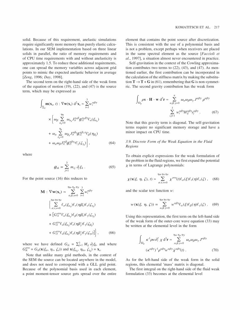
KOMATITSCH ET AL. 217
solid. Because of this requirement, anelastic simulationsrequire significantly more memory than purely elastic calcu-lations. In our SEM implementation based on three linearsolids in parallel, the ratio of memory requirements andof CPU time requirements with and without anelasticity isapproximately 1.5. To reduce these additional requirements,one can spread the memory variables across adjacent gridpoints to mimic the expected anelastic behavior in average[Zeng, 1996; Day, 1998].
The second term on the right-hand side of the weak formof the equation of motion (19), (22), and (47) is the sourceterm, which may be expressed as
�∑s
m(xs, t) : ∇w(xs) d2xs ≈ �3
i=1w���
i
× ��� ���
�s=0��s J�s�
b g�s��i1 �′�(��s)
+ �� ���
�s=0��s J��s
b g��s�i2 �′� (��s)
+ ���� J��b g���s
i3 �′� (��s)� , (64)
where
gik = �3
j=1mij ∂j � k . (65)
For the point source (16) this reduces to
M : ∇w(xs) ≈ ���,��,��
�,�,�=0�3
i=1w���
i
� ���,��,��
�,�,�=0�� (��s)�� (��s)�� (��s)
× �G���i1 �′� (��s)�� (��s)�� (��s)
+ G���i2 ��(��s)�′� (��s)�� (��s)
+ G���i3 ��(��s)�� (��s)�′� (��s)� , (66)
where we have defined Gik = ∑3j=1 Mij ∂j �k, and where
G���ik = Gik(x(��, ��, ��)) and x(��s, ��s, ��s) = xs.
Note that unlike many grid methods, in the context ofthe SEM the source can be located anywhere in the model,and does not need to correspond with a GLL grid point.Because of the polynomial basis used in each element,a point moment-tensor source gets spread over the entire
element that contains the point source after discretization.This is consistent with the use of a polynomial basis andis not a problem, except perhaps when receivers are placedin the same spectral element as the source [Faccioli etal., 1997], a situation almost never encountered in practice.
Self-gravitation in the context of the Cowling approxima-tion contributes two terms to (22), (43), and (47). As men-tioned earlier, the first contribution can be incorporated inthe calculation of the stiffness matrix by making the substitu-tion T → T + G in (61), remembering that G is non-symmet-ric. The second gravity contribution has the weak form
��e
�s · H · w d3r ≈ �n
�,�,�=0������ J��� ����
�3
i,j=1w���
i H���ij s���
j . (67)
Note that this gravity term is diagonal. The self-gravitationterms require no significant memory storage and have aminor impact on CPU time.
3.9. Discrete Form of the Weak Equation in the FluidRegions
To obtain explicit expressions for the weak formulation ofthe problem in the fluid regions, we first expand the potential� in terms of Lagrange polynomials:
� (x(�, �, � ), t) ≈ ���,��,��
�,�,�=0� ���(t)�� (� )��(�)�� (� ) , (68)
and the scalar test function w:
w (x(�, �, � )) = ���,��,��
�,�,�=0w����� (� )�� (�)�� (� ) . (69)
Using this representation, the first term on the left-hand sideof the weak form of the outer-core wave equation (33) maybe written at the elemental level in the form
��e
�-1�w∂ 2t � d3r ≈ �
�� ,�� ,��
�,�,�=0������ J���
(���� )-1����w��� � ���(t) . (70)
As for the left-hand side of the weak form in the solidregions, this elemental ‘mass’ matrix is diagonal.
The first integral on the right-hand side of the fluid weakformulation (33) becomes at the elemental level

218 THE SPECTRAL-ELEMENT METHOD IN SEISMOLOGY
��e
∇w · ∇� d3r ≈ ��� ,�� ,��
�,�,�=0w���
����� ���′
�′=0��′ J�′��
e (∂1�)�′���′�(��′)
+ ���� ���′
�′=0��′ J��′�
e (∂2�)��′��′� (��′)
+ ���� ���′
�′=0��′ J���′
e (∂3�)���′�′� (��′)� , (71)
where
(∂i�)��� = ���
�=0���′�′�′�(��′)∂i�
+ ���
�=0��′��′�′�(��′)∂i�
+ ���
�=0��′�′��′� (��′)∂i� . (72)
The second term on the right-hand side of the weak formof the wave equation in the outer core (33), which arises inthe presence of self-gravitation and rotation, is
��e
�-1�w g · (∇� + u) d3r ≈
�n
�, �, �=0������ J���w���(����)-1����
�3
i=1g���
i [(∂i�)��� + u���i ] , (73)
where (∂i�)���, and where we have made the Cowling ap-proximation.
The weak form of (34) is, in fact, entirely diagonal, whichmeans that one needs to solve a second-order ordinary differ-ential equation at each GLL point. Making the Cowlingapproximation and assuming that N2 = 0 reduces the problemto solving the first-order equation (36), which may be accom-plished based upon a Runge-Kutta scheme, as discussed inKomatitsch and Tromp [2002b].
3.10. Coupling Between Fluid and Solid Regions
The final term on the right-hand side of the weak forms ofthe equation of motion in the solid regions (22), (43), and(47) is the surface integral over the CMB or ICB that repre-sents the interactions in traction and normal velocity between
the solid mantle, the liquid core, and the solid inner core.A key ingredient of our domain decomposition technique isthat, since we have a conforming mesh everywhere, i.e., thegrid points on the CMB are common to the meshes in themantle and in the outer core and the grid points on the ICBare common to the meshes in the outer and inner core, wecan take the value of pressure at a given grid point from thefluid side and use it directly in the surface integral on thesolid side. Therefore, no interpolation is needed at a fluid-solid interface. This type of matching is referred to as point-wise matching in the finite-element literature. At the elemen-tal level on a boundary, the surface integrals over the CMBand the ICB in the solid regions may therefore be ex-pressed as
�p n · wd2x ≈ ���,��
�,�=0���� J��
b p��(t) �3
i=1���
i n��i ,
(74)
where Jb is the surface Jacobian (5), n is the normal (4),and where we calculate the pressure p based upon (37),taking the values of the right-hand side terms from thefluid side.
Similarly, the two surface integrals over the CMB and theICB in the weak form of the equation of motion in the outercore (33) may be expressed as
�w n · s d2x ≈ ���,��
�,�=0���� J��
b w�� �3
i=1s��
i n��i . (75)
3.11. Accuracy of the Method
In a standard FEM, low-degree polynomials (usually of de-gree 1 or 2) are used to discretize functions, and thereforethe accuracy of the method can mainly be adjusted basedupon the typical size of an element in the mesh, �h, i.e.,based upon mesh density. This means that in a traditionalFEM, mesh design is the main parameter that controls accu-racy. In a SEM, however, high-degree Lagrange interpolantsare used to express functions. Therefore, the polynomialdegree used to represent functions on an element, n, is anadditional parameter that can be used to adjust the accuracyof the method.
Even on a unit cube with homogeneous material proper-ties, the GLL numerical integration rule is exact only forpolynomials of degree 2n − 1. Any integration on the refer-ence element involving the product of two polynomials ofdegree n –the displacement and the test function– is neverexact, even in this simplest case. For deformed elementsthere are additional errors related to curvature [Maday andRønquist, 1990]; the same is true for elements with heteroge-

KOMATITSCH ET AL. 219
neous material properties. Thus a diagonal mass matrix isobtained in the Legendre SEM by purposely selectinga numerical integration rule that is not exact (but of coursestill very accurate) for the polynomial basis chosen (a processknown as sub-integration in the finite-element literature). Inthis respect, the SEM is related to FEMs in which masslumping is used to avoid the costly resolution of the non-diagonal system resulting from the use of a Gauss quadraturerule [e.g., Cohen et al., 1993]. As mentioned above, a differ-ent choice is made in the Chebyshev SEM used by someauthors [e.g., Priolo et al., 1994; Seriani, 1998], in whichan integration rule that is exact for the polynomial basischosen is used, with the consequence that the exactly diago-nal mass matrix is lost.
One of the shortcomings of the SEM for elastic media isthat to our knowledge no theoretical analysis of its accuracyis available in the literature. For other classical numericaltechniques such an analysis is usually performed in the spec-tral domain for a regular grid in a homogeneous medium.In the case of the SEM doing so turns out to be challengingbecause the polynomial degree used to discretize the wavefield is high and also because the GLL numerical integrationpoints are non-evenly spaced, which makes it technicallydifficult to use a standard Fourier analysis to perform theaccuracy study, even in the case of a regular mesh of spectralelements in a homogeneous medium. In addition, one of themain ideas behind the use of the SEM is to take advantageof its geometrical flexibility and to therefore use highly-distorted non-regular meshes. On such meshes, performingan accuracy analysis is even more difficult because thereare additional error terms associated with the distortion of themesh elements, as in any finite element or spectral method[Maday and Rønquist, 1990]. To our knowledge, only Tordj-man [1995] and Cohen and Fauqueux [2000] have attemptedsuch a theoretical accuracy study for the SEM in the acousticcase, and Seriani and Priolo [1994] have addressed the issuebased on a numerical study, also in the acoustic case.
Therefore, by trial and error, heuristic rules of thumb haveemerged in order to determine how to select the polynomialdegree to use in practice for an elastic SEM with a non-regular deformed mesh and a heterogeneous medium. Basi-cally, we have used the main conclusions of Seriani andPriolo [1994] in the acoustic case and checked numericallyby performing numerous benchmarks and comparisons toanalytical solutions for simple cases that these conclusionsextend reasonably well to the elastic case. Based on thesenumerical experiments, we can say that using polynomialdegrees lower than typically 4 leads to similar inaccuraciesas with standard FEMs [Marfurt, 1984], i.e., a large amountof numerical dispersion, which means that with such lowdegrees the advantages of using a SEM are lost. In contrast,
if the polynomial degree is very large, e.g., greater than 10,the SEM is spatially very accurate, but the computationalrequirements become prohibitive because of the size of thecalculations related to matrix multiplications involving thefull stiffness matrix, a process with a cost of O(n4) in 3-D,i.e., the numerical cost of the technique becomes prohibitive.Another problem in the case of a high degree is that the non-evenly spaced GLL numerical integration points becomeclustered toward the edges of each spectral element (thespacing between the first two GLL points varies approxi-mately as O(n-2)), and as a result of the small distancebetween these first two points, very small time steps haveto be used to keep the explicit time-marching scheme stable(see Section 4), which drastically increases the cost of theLegendre SEM. Therefore, the rule of thumb is that for mostwave propagation applications, polynomial degrees betweenapproximately 4 and 10 should be used in practice.
In our case, we always use a polynomial degree n = 4. Inorder to obtain accurate results, we use another heuristicrule of thumb that says that for this polynomial degree theaverage grid spacing �h should be chosen such that theaverage number of points per minimum wavelength �min inan element, (n + 1)�min/�h, be roughly equal to 5. It wouldbe of interest to study this more precisely in the 3-D elasticcase based on numerical experiments with different polyno-mial degrees and different values of the grid spacing, andto see how this accuracy analysis would compare to similarstudies for more classical numerical techniques such as thefinite-difference method. Such a comparative study shouldinclude both body and surface waves, the former being moredifficult to model accurately than the latter, in particular formethods that are not based on a variational formulation ofthe wave equation. Schubert [2003] has started to study thisproblem in the 1-D case.
4. TIME INTEGRATION OF THE GLOBAL SYSTEM
In each individual spectral element, functions are sampledat the GLL points of integration. As can be seen in Figure 5,these points include −1 and 1, i.e., each element has gridpoints located exactly on its edges, and therefore sharesthese points (on its faces, edges, or corners) with neighboringelements in the spectral-element mesh. Therefore, as ina classical FEM, we need to distinguish the local mesh ofgrid points inside each element from the global mesh ofpoints in the entire structure, which contains many pointsthat are shared amongst several elements. In addition, thenumber of elements that share a given point (the so-calledvalence of a point) can vary and take any value in the mesh(in other words, the mesh can be non-structured), unlike ina regular mesh of cubes, in which the valence of a shared

220 THE SPECTRAL-ELEMENT METHOD IN SEISMOLOGY
point is always 2 inside a face, 4 on an edge, and 8 at acorner.
Therefore, the first required step is to uniquely numberthe global points in order to define a mapping between thelocal mesh and the global mesh. This can be accomplishedusing efficient finite-element global numbering libraries thateither take advantage of the known and fixed topology ofthe mesh (valence and list of neighbors) to uniquely assigna global point number to each local point inside a givenspectral element, or perform a triple sorting algorithm oneach coordinate of the points (sorting by increasing x, thenby increasing y for the same x, then by increasing z for thesame x and y), again to detect common points and uniquelyassign a global point number to each local point. Once thismapping has been defined, the internal forces computedseparately on each element need to be summed at commongrid points (in the finite-element literature this step is called‘assembling the system’). On a parallel computer, this partis the only step in the SEM that involves communicationsbetween adjacent mesh slices, as we will see in Section 5,because different slices located on different processors canshare common points on their respective edges.
Let U denote the global displacement vector in the solidregions of the model, i.e., U contains the displacement vectorat all the grid points in the global mesh, classically referredto as the global degrees of freedom of the system. The timeevolution of the global system is governed by an ordinarydifferential equation of the general form
MsU + KsU + Bsp = Fs , (76)
where Ms denotes the global diagonal mass matrix, Ks theglobal stiffness matrix, Bsp the fluid-solid coupling terminvolving the pressure p that represents the boundary interac-tions at the CMB or ICB, and Fs the earthquake source term.As mentioned above, one can take advantage of the fact thatthe global mass matrix is diagonal by using a fully explicitsecond-order finite-difference scheme to march this second-order ordinary differential equation, moving the stiffnessterm to the right-hand side. The memory-variable equation(13) is solved for R� using a modified second-order Runge-Kutta scheme in time, since such schemes are known to beefficient for this problem [Carcione, 1994]. We do not spreadthe memory variables across the grid.
In the fluid regions of the model (the outer core in the caseof the global Earth), we similarly get an ordinary differentialequation of the general form:
Mf X + Kf X + Bf U = 0 , (77)
where X is the global potential, Mf denotes the global diago-nal generalized mass matrix, Kf the global generalized stiff-
ness matrix, and Bf U the global fluid-solid coupling terminvolving the solid displacements U that represents theboundary interactions at the CMB or ICB (note that thereis no source term in the fluid because the earthquake sourceis always located in the solid).
Compared to Komatitsch and Tromp [2002a, b], the im-proved formulation in the fluid region developed in Chaljuband Valette [2004] (see also Section 3.3 above) leads to atime-marching scheme in which there is no need to iterateon the fluid-solid coupling condition, i.e., following Chaljuband Valette [2004] we simply first solve (77) in the fluidand then (76) in the solid. The fluid-solid coupling term isevaluated based on the new values on the fluid side computedby solving (77).
The explicit time schemes introduced above are condition-ally stable, i.e., for a given mesh and a given model thereexists an upper limit on the time step above which calcula-tions are unstable. One can define the Courant stability num-ber of the explicit time integration schemes C = �t(v/�h)max,where �t is the time step chosen and (v/�h)max denotesthe maximum ratio of P-wave speed and grid spacing. TheCourant stability condition [Courant et al., 1928] then saysthat the Courant number should not be chosen higher thanan upper limit:
C ≤ Cmax (78)
that determines how large the time step can be while main-taining a stable simulation. Unfortunately, for the SEM toour knowledge there is no published theoretical analysis ofhow to determine the maximum Courant number Cmax. Theheuristic rule of thumb that we use in practice is that forregular meshes Cmax 0.5, while for very irregular mesheswith distorted elements and/or very heterogeneous mediaCmax reduces to approximately 0.3 to 0.4. As for the issueof accuracy in Section 3.11, performing such a theoreticalanalysis for the SEM in the elastic case would be verydifficult, even for a regular mesh in a homogeneous medium,because of the high polynomial degrees used, and becauseof the fact that the GLL numerical integration points arenon-evenly spaced.
5. IMPLEMENTATION ON PARALLEL COMPUTERS
The mesh designed in Section 2 is too large to fit in memoryon a single computer. Modern parallel computers such asclusters or grids of computers have a distributed memoryarchitecture. The standard approach for programming paral-lel machines with distributed memory in a portable way isto use a message-passing methodology, usually based upon

KOMATITSCH ET AL. 221
a library called MPI [e.g., Gropp et al., 1994], an acronymfor ‘Message Passing Interface’.
Because we use an explicit time-marching scheme (seeSection 4), our SEM algorithm mostly consists in smalllocal matrix-vector products in each spectral element, whichimplies that the processors spend most of their time doingactual calculations, and only a small amount of time in thecommunication step. Hence, the SEM algorithm is not verysensitive to the speed of the network connecting the differentprocessors. It can therefore run on high-latency networkssuch as clusters of PC computers, sometimes referred to as‘Beowulf’ machines, or on grids of computers.
In order to run an SEM algorithm on such parallel ma-chines, we need to split the mesh into as many slices as thenumber of processors we use on the machine. Plate 1 showshow the mesh of Figure 3 for the global Earth is split intoslices in the case of calculations distributed over 1944 proc-essors (6 chunks of 18 × 18 slices each), as will be used inSection 6. Calculations can be performed locally by eachprocessor on the spectral elements that constitute the meshslice it carries, and one communication phase is then requiredat each time step of our time-marching algorithm in orderto sum the internal forces computed at the common faces,edges, and corners shared by mesh slices carried by differentprocessors. Therefore, MPI communication tables that or-chestrate the (constant) sequence of messages that needs tobe exchanged amongst the slices at each time step need tobe created once and for all when the mesh is built.
6. NUMERICAL RESULTS
In previous work, synthetic seismograms for 3-D Earth mod-els calculated based on the SEM have been successfullycompared to broadband data, both for sedimentary basins[Komatitsch et al., 2004; Liu et al., 2004] and at a globalscale [Komatitsch and Tromp, 2002b; Chaljub et al., 2003;Komatitsch et al., 2003; Tsuboi et al., 2003; Capdeville etal., 2003]. Here, as an application of the SEM to a large-scale 3-D problem, we combine all the complications ofa fully 3-D Earth model. The simulations include anisotropy(the reference 1-D PREM upper mantle model is anisotropic,see Komatitsch and Tromp [2002a] for details), attenuation,self-gravitation, the oceans, rotation, ellipticity, topographyand bathymetry, a 3-D mantle model and a 3-D model ofcrustal wave speeds, as explained in Section 2 (see alsoKomatitsch and Tromp [2002b] for more details on thesemodels).
The SEM calculations are performed on the Earth Simula-tor at the Japan Agency for Marine Earth Science and Tech-nology (JAMSTEC). This computer has 640 8-processorcompute nodes, for a total of 5120 processors. Each node
has 16 gigabytes of shared memory, for a total of 10 terabytesof memory. The peak performance per node is 64 gigaflops(i.e., 64 billions of floating-point operations per second) andthe total peak performance is 40 teraflops. On 48 nodes ofthe Earth Simulator we can model periods of 9 s anda typical simulation lasts 10 hours, 243 Earth Simulatornodes enable us to reach periods of 5 s, and on 507 nodes thisis further reduced to a shortest period of 3.5 s [Komatitsch etal., 2003; Tsuboi et al., 2003]. To put these numbers inperspective, typical normal-mode summation codes that cal-culate semi-analytical synthetic seismograms for 1-D Earthmodels are accurate down to 6 s. In other words, the EarthSimulator allows us to simulate global seismic wave propa-gation in fully 3-D Earth models at periods shorter thancurrent seismological practice for 1-D spherically symmetricmodels.
We model the September 2, 1997, 210 km deep Colombiaearthquake, which had a magnitude of Mw = 6.7. We usethe mesh in Figures 3, 4 and Plate 1 and a polynomial degreen = 4, which gives a grid composed of 82 million spectralelements and a total of 14.5 billion grid points. At the surfaceof the model the size of the spectral elements is 1.04° in thetwo horizontal directions (i.e., the average spacing betweenadjacent grid points is 0.026°, or equivalently 2.9 km). Thetime step is �t = 72 ms, and we propagate the signal for3600 s. Receivers from the global network of seismic stationsrecord the three components of displacement. Figure 7 showsthe results of a simulation on the Earth Simulator accuratedown to 5 s. The source is the CMT solution taken fromthe Harvard catalog. The vertical component data are linedup on the Rayleigh wave. Note the remarkable fit both atshort and long periods. In Figure 8 we present the sameresults centered on the P-wave arrival. Note the distinctpP and sP arrivals, and also note that the sP arrivals areconsistently late in the SEM synthetic seismograms, whichimplies that the shear wave speed model we use is too slowin the mantle wedge above the subducting plate.
In the case of large earthquakes, the finite size of theearthquake source must be taken into account, and an equiva-lent CMT cannot be used. Plate 2 shows a snapshot of sucha finite-fault simulation for the November 3, 2002, Denalifault, Alaska, earthquake, which had a magnitude of Mw =7.9 and ruptured several fault segments over a total distanceof 220 km [Eberhart-Phillips et al., 2003]. The finite sourcemodel, which is represented by 475 point double couplesolutions, was determined by Ji et al. [2004]. Because theearthquake rupture propagates in a southeasterly directionalong the Denali fault, the waves that propagate along theWest coast of the United States have large amplitudes. Thisdirectivity effect due to the finite size of the earthquake faultis captured well by the SEM simulations. We show full

222 THE SPECTRAL-ELEMENT METHOD IN SEISMOLOGY
Plate 1. The spectral-element method uses a mesh of hexahedralfinite elements on which the wave field is interpolated by high-degree Lagrange polynomials on Gauss-Lobatto-Legendre integra-tion points. In order to perform the calculations on a parallel com-puter with distributed memory, the mesh in Figures 3 and 4 is splitinto slices based upon a regular domain-decomposition topology.Each slice is handled by a separate processor. Adjacent sliceslocated on different processors exchange information about com-mon faces and edges based upon a message-passing methodology.The top figure shows a global view of the mesh at the surface,illustrating that each of the six sides of the so-called ‘cubed sphere’mesh is divided into 18 × 18 slices, shown here with differentcolors, for a total of 1944 slices. The bottom figure shows a close-up of the mesh of 48 × 48 spectral elements at the surface of eachslice. Within each surface spectral element we use 5 × 5 = 25 Gauss-Lobatto-Legendre grid points, which translates into an average gridspacing of 2.9 km (i.e., 0.026°) on the entire Earth surface.
Plate 2. Snapshot of the propagation of seismic waves in theEarth generated by the November 3, 2002 Denali fault, Alaska,earthquake. Note the large amplification of the waves along thewestern coast of the United States.

KOMATITSCH ET AL. 223
Figure 7. Comparison of vertical component data (solid line) andspectral-element synthetic seismograms (dashed line) for the Sep-tember 2, 1997, 210 km deep Colombia earthquake. Both thesynthetic seismograms and the data are lowpass-filtered at 5 s. Thesource azimuth measured clockwise from due North is indicatedon the left, and the station name and epicentral distance are on theright. Records are aligned on the Rayleigh wave.
waveform comparisons between data and synthetic seismo-grams in Figure 9. Note that the SEM synthetic seismogramscapture the dispersion of the Rayleigh waves remarkablywell.
7. CONCLUSIONS
We have presented a detailed description of the spectralelement method for 3-D seismic wave propagation. Thefull complexity of Earth models, i.e., surface topography,attenuation, anisotropy and fluid-solid interfaces, and, in thecase of global simulations, self-gravitation, rotation and theoceans, are taken into account. We have used an improvedSEM formulation for the outer core in the presence of self-gravitation and rotation that has the important benefit thatit does not require iterations on the fluid-solid coupling
Figure 8. Comparison of vertical component data (solid line) andspectral-element synthetic seismograms (dashed line) for the Sep-tember 2, 1997, 210 km deep Colombia earthquake. Both thesynthetic seismograms and the data are lowpass-filtered at 5 s. Thesource azimuth measured clockwise from due North is indicatedon the left, and the station name and epicentral distance are on theright. Records are aligned on the P wave. Note the distinct pP andsP arrivals at 60 s and 80 s after the P wave, respectively. Theamplitudes in this plot are more than ten times smaller than thosein Figure 7.
condition at the CMB or at the ICB, thus making the SEMalgorithm much simpler and more efficient numerically. Themethod has been implemented on a parallel computer withdistributed memory based upon a message-passing method-ology.
In the current implementation we make the Cowling ap-proximation, make the assumption that the Brunt-Vaisalafrequency is zero, use an approximate treatment of the effectof the oceans, and rely on a simple one-way treatment forabsorbing boundaries in the case of regional or local simula-tions. Effects of the Cowling approximation and a non-zero Brunt-Vaisala frequency are only relevant at very longperiods (typically > 500 s). Improved implementations of

224 THE SPECTRAL-ELEMENT METHOD IN SEISMOLOGY
Figure 9. Comparison of vertical component data (solid line) andspectral-element synthetic seismograms (dashed line) for the No-vember 3, 2002, Denali fault, Alaska, earthquake. Both the syn-thetic seismograms and the data are lowpass-filtered at 5 s. Thesource azimuth measured clockwise from due North is indicatedon the left, and the station name and epicentral distance are on theright. Records are aligned on the P wave.
the oceans are under investigation and will be the focus offuture work.
We have used the Japanese Earth Simulator to performa direct comparison between synthetic seismograms calcu-lated for a realistic fully 3-D Earth model and observedseismograms for two large earthquakes. This comparisonshows that our spectral-element simulations capture generalfeatures of the Earth’s 3-D structure fairly well. However,it is also apparent that the agreement between synthetic andobserved seismograms decreases at high frequency due to thefact that current 3-D Earth models are not well constrained atsuch high frequencies.
In the near future, we believe that the SEM will becomethe method of choice for the simulation of seismic wavepropagation in fully 3-D Earth models. The main difficultyis the cost of large simulations, as is the case for all methods
that are based upon the full wave equation discretized ona grid. However, because of the continuous evolution ofcomputer technology, a small group of researchers can nowassemble a PC cluster at a reasonable cost in a reasonableamount of time and perform large-scale 3-D simulations in-house, and at the same time, very large machines such as theEarth Simulator in Japan or large geographically-distributednetworks of clusters of computers (known as GRIDs) startto provide enough memory and processors to run complexmodels at unprecedented resolution. This has already led toCentroid-Moment Tensor (CMT) source inversion in fully3-D Earth models [Liu et al., 2004], opening the door tofull waveform tomographic inversions.
The full source code of our program SPECFEM3D isfreely available for academic, non-commercial research fromwww.geoframework.org.
Acknowledgments. The authors would like to thank Chen Ji foruse of his finite-fault source model for the Denali earthquake.Dimitri Komatitsch also thanks Emmanuel Chaljub, Jean-PierreVilotte, Yvon Maday, Anthony T. Patera, Geza Seriani, EnricoPriolo, Fabio Cavallini and Alain Bamberger for enlightening dis-cussions about spectral-element and finite-element methods. Thethorough and constructive comments of two anonymous reviewersand editors Alan Levander and Guust Nolet improved the manu-script. Simulations on the Earth Simulator were performed underthe collaborative project of the Earth Simulator Center entitled‘Global elastic response simulation’. Broadband data were obtainedfrom the IRIS Data Management Center. This material is based inpart upon work supported by the National Science Foundationunder grant EAR-0309576. This is contribution No. 9076 of theDivision of Geological & Planetary Sciences, California Instituteof Technology, USA.
REFERENCES
Anderson, D. L., A seismic equation of state, Part II: Shear proper-ties and thermodynamics of the lower mantle, Phys. Earth Planet.Inter., 45, 307–323, 1987.
Bao, H., J. Bielak, O. Ghattas, L. F. Kallivokas, D. R. O’Hallaron,J. R. Shewchuk, and J. Xu, Large-scale simulation of elasticwave propagation in heterogeneous media on parallel computers,Comput. Methods Appl. Mech. Engrg., 152, 85–102, 1998.
Bassin, C., G. Laske, and G. Masters, The current limits of resolu-tion for surface wave tomography in North America, EOS, 81,F897, 2000.
Basu, U., and A. K. Chopra, Perfectly matched layers for transientelastodynamics of unbounded domains, Int. J. Numer. Meth.Engng., 59, 1039–1074, 2004.
Berenger, J. P., A Perfectly Matched Layer for the absorption ofelectromagnetic waves, J. Comput. Phys., 114, 185–200, 1994.
Bouchon, M., C. A. Schultz, and M. N. Toksoz, Effect of three-dimensional topography on seismic motion, J. Geophys. Res.,101, 5835–5846, 1996.

KOMATITSCH ET AL. 225
Canuto, C., M. Y. Hussaini, A. Quarteroni, and T. A. Zang, Spectralmethods in fluid dynamics, Springer-Verlag, New York, 1988.
Capdeville, Y., E. Chaljub, J. P. Vilotte, and J. P. Montagner,Coupling the spectral element method with a modal solution forelastic wave propagation in global Earth models, Geophys. J.Int., 152, 34–67, 2003.
Carcione, J. M., The wave equation in generalized coordinates,Geophysics, 59, 1911–1919, 1994.
Carcione, J. M., D. Kosloff, and R. Kosloff, Wave propagationsimulation in a linear viscoelastic medium, Geophys. J. Int., 95,597–611, 1988.
Chaljub, E., Modelisation numerique de la propagation d’ondessismiques en geometrie spherique : application a la sismologieglobale (Numerical modeling of the propagation of seismicwaves in spherical geometry: application to global seismology),Ph.D. thesis, Universite Paris VII Denis Diderot, Paris, France,2000, in French.
Chaljub, E., and B. Valette, Spectral element modelling of three-dimensional wave propagation in a self-gravitating Earth withan arbitrarily stratified outer core, Geophys. J. Int., 158, 131–141, 2004.
Chaljub, E., Y. Capdeville, and J. P. Vilotte, Solving elastodynam-ics in a fluid-solid heterogeneous sphere: a parallel spectralelement approximation on non-conforming grids, J. Comput.Phys., 187, 457–491, 2003.
Clayton, R., and B. Engquist, Absorbing boundary conditions foracoustic and elastic wave equations, Bull. Seismol. Soc. Am.,67, 1529–1540, 1977.
Cohen, G., and S. Fauqueux, Mixed finite elements with masslumping for the transient wave equation, J. Comput. Acoust., 8,171–188, 2000.
Cohen, G., P. Joly, and N. Tordjman, Construction and analysisof higher-order finite elements with mass lumping for the waveequation, in Proceedings of the second international conferenceon mathematical and numerical aspects of wave propagation,edited by R. Kleinman, pp. 152–160, SIAM, Philadephia, PA,1993.
Collino, F., and C. Tsogka, Application of the PML absorbinglayer model to the linear elastodynamic problem in anisotropicheterogeneous media, Geophysics, 66, 294–307, 2001.
Courant, R., K. O. Friedrichs, and H. Lewy, Uber die partiellenDifferenzengleichungen der mathematischen Physik, Mathema-tische Annalen, 100, 32–74, 1928, in German.
Cowling, T. G., The non-radial oscillations of polytropic stars,Mon. Not. Roy. Astron. Soc., 101, 369–373, 1941.
Dahlen, F. A., and J. Tromp, Theoretical Global Seismology,Princeton University Press, Princeton, 1998.
Day, S. M., Efficient simulation of constant Q using coarse-grainedmemory variables, Bull. Seismol. Soc. Am., 88, 1051–1062, 1998.
Dziewonski, A. M., and D. L. Anderson, Preliminary referenceEarth model, Phys. Earth Planet. Inter., 25, 297–356, 1981.
Eberhart-Phillips, D., et al., The 2002 Denali fault earthquake,Alaska: a large magnitude, slip-partitioned event, Science, 300,1113–1118, 2003.
Emmerich, H., and M. Korn, Incorporation of attenuation into time-domain computations of seismic wave fields, Geophysics, 52,1252–1264, 1987.
Faccioli, E., F. Maggio, R. Paolucci, and A. Quarteroni, 2D and3D elastic wave propagation by a pseudo-spectral domain de-composition method, J. Seismol., 1, 237–251, 1997.
Festa, G., and J. P. Vilotte, The Newmark scheme as velocity-stresstime-staggering: an efficient PML implementation for spectralelement simulations of elastodynamics, Geophys. J. Int., 161,789-812, doi:10.1111/j.1365-246X.2005.02601.x, 2005.
Graves, R. W., Simulating seismic wave propagation in 3D elasticmedia using staggered-grid finite differences, Bull. Seismol. Soc.Am., 86, 1091–1106, 1996.
Gropp, W., E. Lusk, and A. Skjellum, Using MPI, portable parallelprogramming with the Message-Passing Interface, MIT Press,Cambridge, 1994.
Guo, B., and I. Babuska, The h-p version of the finite elementmethod, Comput. Mech., 1, 21–41, 1986.
Hughes, T. J. R., The finite element method, linear static anddynamic finite element analysis, Prentice-Hall International, En-glewood Cliffs, NJ, 1987.
Ji, C., D. V. Helmberger, and D. J. Wald, A teleseismic study ofthe 2002 Denali fault, Alaska, earthquake and implications forrapid strong-motion estimation, Earthquake Spectra, 20, 617–637, 2004.
Karato, S., Importance of anelasticity in the interpretation of seis-mic tomography, Geophys. Res. Lett., 20, 1623–1626, 1993.
Kawase, H., Time-domain response of a semi-circular canyon forincident SV, P and Rayleigh waves calculated by the discretewavenumber boundary element method, Bull. Seismol. Soc. Am.,78, 1415–1437, 1988.
Kennett, B. L. N., and E. R. Engdahl, Traveltimes for globalearthquake location and phase identification, Geophys. J. Int.,105, 429–465, 1991.
Komatitsch, D., Methodes spectrales et elements spectraux pourl’equation de l’elastodynamique 2D et 3D en milieu heterogene(Spectral and spectral-element methods for the 2D and 3D elasto-dynamics equations in heterogeneous media), Ph.D. thesis, Insti-tut de Physique du Globe, Paris, France, 1997, in French, 187pages.
Komatitsch, D., and J. Tromp, Introduction to the spectral-elementmethod for 3-D seismic wave propagation, Geophys. J. Int., 139,806–822, 1999.
Komatitsch, D., and J. Tromp, Spectral-element simulations ofglobal seismic wave propagation-I. Validation, Geophys. J. Int.,149, 390–412, 2002a.
Komatitsch, D., and J. Tromp, Spectral-element simulations ofglobal seismic wave propagation-II. 3-D models, oceans, rota-tion, and self-gravitation, Geophys. J. Int., 150, 303–318, 2002b.
Komatitsch, D., and J. Tromp, A Perfectly Matched Layer ab-sorbing boundary condition for the second-order seismic waveequation, Geophys. J. Int., 154, 146–153, 2003.
Komatitsch, D., and J. P. Vilotte, The spectral-element method:an efficient tool to simulate the seismic response of 2D and 3Dgeological structures, Bull. Seismol. Soc. Am., 88, 368–392,1998.
Komatitsch, D., C. Barnes, and J. Tromp, Wave propagation neara fluid-solid interface: a spectral element approach, Geophysics,65, 623–631, 2000a.

226 THE SPECTRAL-ELEMENT METHOD IN SEISMOLOGY
Komatitsch, D., C. Barnes, and J. Tromp, Simulation of anisotropicwave propagation based upon a spectral element method, Geo-physics, 65, 1251–1260, 2000b.
Komatitsch, D., R. Martin, J. Tromp, M. A. Taylor, and B. A.Wingate, Wave propagation in 2-D elastic media using a spectralelement method with triangles and quadrangles, J. Comput.Acoust., 9, 703–718, 2001.
Komatitsch, D., J. Ritsema, and J. Tromp, The spectral-elementmethod, Beowulf computing, and global seismology, Science,298, 1737–1742, 2002.
Komatitsch, D., S. Tsuboi, C. Ji, and J. Tromp, A 14.6 billiondegrees of freedom, 5 teraflops, 2.5 terabyte earthquake simula-tion on the Earth Simulator, Proceedings of the ACM/IEEESupercomputing SC’2003 conference, 2003, published on CD-ROM and at www.sc-conference.org/sc2003.
Komatitsch, D., Q. Liu, J. Tromp, P. Suss, C. Stidham, and J. H.Shaw, Simulations of ground motion in the Los Angeles basinbased upon the spectral-element method, Bull. Seismol. Soc. Am.,94, 187–206, 2004.
Liu, H. P., D. L. Anderson, and H. Kanamori, Velocity dispersiondue to anelasticity: implications for seismology and mantle com-position, Geophys. J. R. Astron. Soc., 47, 41–58, 1976.
Liu, Q., J. Polet, D. Komatitsch, and J. Tromp, Spectral-elementmoment-tensor inversions for earthquakes in Southern Califor-nia, Bull. Seismol. Soc. Am., 94, 1748–1761, 2004.
Madariaga, R., Dynamics of an expanding circular fault, Bull.Seismol. Soc. Am., 65, 163–182, 1976.
Maday, Y., and E. M. Rønquist, Optimal error analysis of spectralmethods with emphasis on non-constant coefficients and de-formed geometries, Comput. Methods Appl. Mech. Engrg., 80,91–115, 1990.
Marfurt, K. J., Accuracy of finite-difference and finite-elementmodeling of the scalar wave equation, Geophysics, 49, 533–549, 1984.
Moczo, P., E. Bystricky, J. Kristek, J. M. Carcione, and M. Bou-chon, Hybrid modeling of P-SV seismic motion at inhomoge-neous viscoelastic topographic structures, Bull. Seismol. Soc.Am., 87, 1305–1323, 1997.
Ohminato, T., and B. A. Chouet, A free-surface boundary conditionfor including 3D topography in the finite difference method,Bull. Seismol. Soc. Am., 87, 494–515, 1997.
Patera, A. T., A spectral element method for fluid dynamics: lami-nar flow in a channel expansion, J. Comput. Phys., 54, 468–488, 1984.
Priolo, E., J. M. Carcione, and G. Seriani, Numerical simulationof interface waves by high-order spectral modeling techniques,J. Acoust. Soc. Am., 95, 681–693, 1994.
Quarteroni, A., A. Tagliani, and E. Zampieri, Generalized Galerkinapproximations of elastic waves with absorbing boundary condi-tions, Comput. Methods Appl. Mech. Engrg., 163, 323–341,1998.
Ritsema, J., H. J. Van Heijst, and J. H. Woodhouse, Complex shearvelocity structure imaged beneath Africa and Iceland, Science,286, 1925–1928, 1999.
Robertsson, J. O. A., A numerical free-surface condition for elastic/viscoelastic finite-difference modeling in the presence of topog-raphy, Geophysics, 61, 1921–1934, 1996.
Ronchi, C., R. Ianoco, and P. S. Paolucci, The ‘‘Cubed Sphere’’:a new method for the solution of partial differential equationsin spherical geometry, J. Comput. Phys., 124, 93–114, 1996.
Sadourny, R., Conservative finite-difference approximations of theprimitive equations on quasi-uniform spherical grids, MonthlyWeather Review, 100, 136–144, 1972.
Sanchez-Sesma, F. J., and M. Campillo, Diffraction of P, SV andRayleigh waves by topographic features: a boundary integralformulation, Bull. Seismol. Soc. Am., 81, 2234–2253, 1991.
Schubert, B., The spectral-element method for seismic wave propa-gation: theory, implementation and comparison to finite differ-ence methods, Tech. rep., University of Munich, Germany, 2003,unpublished report, 165 p.
Seriani, G., A parallel spectral element method for acoustic wavemodeling, J. Comput. Acoust., 5, 53–69, 1997.
Seriani, G., 3-D large-scale wave propagation modeling by a spec-tral element method on a Cray T3E multiprocessor, Comput.Methods Appl. Mech. Engrg., 164, 235–247, 1998.
Seriani, G., and E. Priolo, A spectral element method for acousticwave simulation in heterogeneous media, Finite Elements inAnalysis and Design, 16, 337–348, 1994.
Sherwin, S. J., and G. E. Karniadakis, A triangular spectral elementmethod: applications to the incompressible Navier-Stokes equa-tions, Comput. Methods Appl. Mech. Engrg., 123, 189–229,1995.
Taylor, M., J. Tribbia, and M. Iskandarani, The spectral elementmethod for the shallow water equation on the sphere, J. Comput.Phys., 130, 92–108, 1997.
Taylor, M. A., and B. A. Wingate, A generalized diagonal massmatrix spectral element method for non-quadrilateral elements,Appl. Num. Math., 33, 259–265, 2000.
Tessmer, E., D. Kessler, D. Kosloff, and A. Behle, Multi-domainChebyshev-Fourier method for the solution of the equationsof motion of dynamic elasticity, J. Comput. Phys., 100, 355–363, 1992.
Tordjman, N., Elements finis d’ordre eleve avec condensation demasse pour l’equation des ondes (High-order finite elementswith mass lumping for the wave equation), Ph.D. thesis, Uni-versite Paris IX Dauphine, Paris, France, 1995, in French.
Tsuboi, S., D. Komatitsch, C. Ji, and J. Tromp, Spectral-elementsimulations of the November 3, 2002, Denali, Alaska earthquakeon the Earth Simulator, Phys. Earth Planet. Inter., 139, 305–313, 2003.
Valette, B., About the influence of prestress upon the adiabaticperturbations of the Earth, Geophys. J. R. Astron. Soc., 85, 179–208, 1986.
Valette, B., Spectre des oscillations libres de la Terre: aspectsmathematiques et geophysiques (Spectrum of the free oscilla-tions of the Earth: mathematical and geophysical aspects), Habil-itation thesis, Universite Paris VI Jussieu, Paris, 1987, thesed’etat, in French.
Virieux, J., P-SV wave propagation in heterogeneous media: veloc-ity-stress finite-difference method, Geophysics, 51, 889–901,1986.
Zeng, X., Finite difference modeling of viscoelastic wave propaga-tion in a generally heterogeneous medium in the time domain,

KOMATITSCH ET AL. 227
and a dissection method in the frequency domain, Ph.D. thesis,University of Toronto, Canada, 1996.
Zienkiewicz, O. C., The finite element method in engineering sci-ence, 3rd ed., McGraw-Hill, New York, 1977.
Zingg, D. W., Comparison of high-accuracy finite-differencemethods for linear wave propagation, SIAM Journal onScientific Computing, 22, 476–502, 2000, doi: 10.1137/S1064827599350320.
Zingg, D. W., H. Lomax, and H. Jurgens, High-accuracy finite-difference schemes for linear wave propagation, SIAM Journalon Scientific Computing, 17, 328–346, 1996, doi: 10.1137/S1064827594267173.
Dimitri Komatitsch, CNRS FRE 2639, Universite de Pau et desPays de l’Adour, Avenue de l’Universite, 64013 Pau Cedex, France.(e-mail: [email protected])
Seiji Tsuboi, Institute for Research on Earth Evolution, JapanAgency for Marine-Earth Science and Technology, 3173-25Showa-machi, Kanazawa-ku, Yokohama 236-0001, Japan. (e-mail:[email protected])
Jeroen Tromp, Seismological Laboratory, 1200 East CaliforniaBoulevard, California Institute of Technology, Pasadena, California91125, USA. (e-mail: [email protected])

![The Spectral-Element Method in Seismologyshearer/227C/spec_elem... · 2007-12-27 · 206 THE SPECTRAL-ELEMENT METHOD IN SEISMOLOGY global [e.g., Tessmer et al., 1992] seismic wave](https://static.fdocuments.in/doc/165x107/5f07ef947e708231d41f8046/the-spectral-element-method-in-seismology-shearer227cspecelem-2007-12-27.jpg)