Journal of Non-Newtonian Fluid Mechanics, 26 (1987) 57-76 Elsevier Science Publishers B.V., Amsterdam - Printed in The Netherlands

57

THE SPATIAL DEVELOPMENT OF TRANSIENT COUE’-ITE FLOW AND SHEAR WAVE PROPAGATION IN POLYMERIC LIQUIDS BY FLOW BIREFRINGENCE

J.S. LEE and G.G. FULLER

Dept. of Chemical Engineering, Stanford University, Stanford CA 94305-5025 (U.S.A.)

(Received April 12, 1987)

Summary

In this paper the method of polarization modulated flow birefringence is used to analyze the spatial and temporal dependence of the inception and cessation of Couette flow of polymeric liquids. Data are presented for both a Newtonian but birefringent polybutene oil and two solutions of poly(oxyethylene). The stress-optical rule is used to obtain the correspond- ing shear and normal stresses as functions of both time and space. The data for the Newtonian fluid are compared with analytical solutions to the momentum equations and are found to accurately follow the theoretical predictions. The polymer solutions, on the other hand, show a complex response with evidence for shear stress propagation as a wave of finite, constant speed. The measured wave speeds agree well with recent data reported by Joseph, Riccius and Amey [JFM 171(1986)309] on the same polymer solutions.

1. Introduction

The study of the development of flow fields in a liquid initially at rest has a long history and represents an important rheological test for complex fluids. Work in this field dates back to Stokes’ solution of the flow field of a Newtonian fluid near an accelerating plate in an infinite fluid [l] and has since been extended by numerous workers to other geometries [l-3]. Of interest here, however, is the stress field development of non-Newtonian liquids in space and time. The additional complication of visco-elasticity causes profound, qualitative changes in the response, and phenomena such as wave and shock formation have been both speculated on and observed.

0377-0251/87/$03.50 0 1987 Elsevier Science Publishers B.V.

58

The theoretical analysis of the Rayleigh problem for non-Newtonian fluids include the work of Tanner [4), Joseph et al. [5,6], Mochimaru [7] and Kazakia and Rivlin [3]. The general finding of these researchers is that for fluids with elasticity, discontinuities from solid boundaries will in general propagate waves that travel at a speed c = (G(O)/p)l/’ where G(0) is the initial value of the relaxation modulus, and p is the density. Purely viscous fluids, on the other hand, are diffusive.

Although the details of the dynamics following the inception or cessation of flow can show important structural information about the material being tested, in most instances where such impulsive flows are used as rheological tests, it is simply assumed that the kinematics of the flow are established instantaneously. The purpose of this paper is to describe the use of flow birefringence to measure the spatial dependence of time dependent, inhomo- geneous flows and its application to the problem of the development of plane Couette flow.

Flow birefringence refers to the measurement of flow-induced anisotropy in the refractive index of a liquid and has been used extensively to provide determinations of the microstructure of rheologically complex materials. The value of this measurement is especially important for those cases where the stress-optical rule [S] is known to apply. This rule, which has been shown to have a remarkably wide range of validity, states that the stress and refractive index tensors are related through the following linear relationship

~=CT+AI (1)

where C is the stress-optical coefficient and is independent of polymer concentration and molecular weight. Until recently, however, the experimen- tal methods available for flow birefringence measurements were generally restricted to steady-state and spatially homogeneous flows. However, with the development of techniques such as two-color flow birefringence [9] and polarization modulated flow birefringence [lo], it is now possible to take advantage of the potential of optical methods to perform highly localized measurements of the stress fields in inhomogeneous and time-dependent flows.

2. Experimental apparatus, materials, and procedure

2. I Polarization modulated jlow birefringence

The application of hydrodynamic forces onto a polymeric liquid will generally cause the refractive index tensor to become anisotropic with principal values n, and n2 oriented at an angle x relative to the laboratory axis (normally the flow direction) as depicted in Fig. 1. The difference in

59

l X flow direction

P2

Fig. 1. Optical axes of components making up the optical system.

these principal values An = n, - n2 is referred to as the birefringence and x is the orientation angle. These optical quantities are connected to compo- nents of the stress tensor by eqn. (1) and can be used to calculate the shear stress and first normal stress difference in the following way:

An sin 2x = 2Cr,, (2.1)

An cos 2x = C( 7,. - rY,,) (2.2)

To properly characterize the optical anisotropy of a fluid subjected to a time-dependent, inhomogeneous flow, it is necessary to simultaneously determine the birefringence and the orientation angle. The techniques of two-color flow birefringence and polarization modulated flow birefringence were specifically designed to achieve this capability and the latter method was employed in this study.

The apparatus is described schematically in Fig. 2 and is a simpler version of an apparatus described in detail in Ref. [lo]. The optical components were mounted onto an optical rail system that could be translated indepen- dently of the flow cell. A He-Ne laser (5 mW) was used to generate light at a wavelength of h = 633 run. The light was first passed through a polarizer Pl that had its polarization vector set parallel to the direction of flow. All other orientations for other optical devices in the system are referenced to this direction. Following the first polarizer, the light was sent through a photo-elastic modulator (PEM) and a quarter wave plate (Ql) before pass- ing through the sample (S). The light is then sent through an additional quarter wave plate (42) and polarizer (P2). The orientation of these devices are: (Pl: 0”), (PEM: 45”), (Ql: O”), (42: 0”), (P2: -45’). These orientations are shown in Fig. 1.

60

Pl

PEM PEM CONTROLLER

ADT Q 1

r-l

D $ INTENSITY SIGNAL J

Fig. 2. Experimental apparatus. L = laser He-Ne; Pl, P2 = polarizers, PEM = photoelastic modulator, Ql, 42 = quarter wave plates, S = flow cell, D = detector, C/B = clutch/brake, ADT = angular displacement transducer, M = motor, A = amplifier, LIl, L12 = lock-in amplifiers, LPF= low pass filter, Rl, R2 = ratio circuits. Darkened components are on the optical rail.

The photo-elastic modulator consists of a quartz crystal that is sinusoid- ally strained at a frequency of w = 42.1 kHz that results in a retardation of the light passing through this element of

6 rEM = A sin wt

The intensity of light measured at the detector D can be shown to be

I = 2 [I + sin 2x sin 6 cos S,, + cos 2x sin 6 sin 6,,,] (4)

where I, is the light intensity incident on the PEM, 6 = 2rrAnJ/X is the retardation of the sample and d is the sample thickness.

The signal from the detector is sent to two lock-in amplifiers and a low pass filter. One amplifier is locked to the fundamental frequency of the PEM whereas the second amplifier is locked to twice this frequency. Ratios are then performed of the amplifier signals divided by the DC component measured by the low pass filter. These ratios are measured and stored using

61

a digital storage oscilloscope. Following Ref. (lo), these ratios are the following functions of the sample retardation and orientation angle:

R,, = 24(A) cos 2x sin S (5-l)

R,, = 2.4 (A) sin 2x sin 6 (5 -2)

where Jr(A) and J2( A) are Bessel functions of the PEM retardation ampli- tude and are determined through a straightforward calibration procedure outlined in Ref. [lo]. The measurement of these two ratios provides enough information to calculate the unknown retardation and orientation of the sample. Following that determination, the shear stress and first normal stress difference can be calculated using eqns. (2.1) and (2.2). Measurements can be made at a rate of 1 kHz.

2.2 The Couette flow cell

Figure 3 is a diagram of the Couette flow cell used in the experiments. The basic design of this flow cell is similar to those constructed previously by Tsvetkov [ll]. This design avoids the problems of mechanical friction and

Incidc It Beam

Fig. 3. Couette flow cell.

62

parasitic strain birefringence of the windows present in many other designs by keeping the windows stationary. This is done by using a system of three concentric cylinders of which the second cylinder is rotated to induce the flow. The light for the birefringence measurement is sent through the gap between the inner most cylinder and the rotating second cylinder. Four V-guide wheels support the weight of the rotating cylinder and rotate with little friction. Timing pulleys and belts are used to transfer power from the motor to the flow cell to minimize slippage. The bottom of each cylinder is made in a V-shape to help the release of air bubbles trapped in the bottom of the flow cell. To make the curvature effect inherent to the circular Couette cell small, the outer radius of the inner cylinder (5.64 cm) is about 8 times bigget, ;‘lan the gap width (0.71 cm). This gap is also large relative to the diameter of the laser beam that is nominally 0.08 cm.

To provide precise motion control and synchronization with the data acquisition unit (a digital oscilloscope), a stepping motor capable of 25000 steps/revolution was used to drive the cell. An electro-magnetic clutch/brake assembly was installed between the motor and the flow cell to allow a rapid start-up and cessation of the motion of the rotating cylinder of the Couette flow cell. This is shown in Figure 2.

Although the clutch/brake unit is capable of rapid engagement, mechani- cal compliance and acceleration will lead to imperfect step functions in the velocity of the rotating cylinder as a function of time? For this reason, an angular displacement transducer was fixed to the upper timing pulley of the clutch/brake unit. The signal from this device was acquired simultaneously along with the output of the ratio circuits discussed in the previous section. By differentiating the output voltage from the displacement transducer with respect to time, the angular velocity of the rotating cylinder could be directly calculated.

2.3 Materials

The instrument described above was first-tested using a Newtonian, but birefringent liquid and then applied to two non-Newtonian polymer solu- tions. The Newtonian fluid was a low molecular weight polybutene liquid, PB8, manufactured by Chevron. This material has a number average molec- ular weight of 440 g mol-’ and a viscosity of 2.65 poise (265 mPa . s) at 21 o C. The characteristic vorticity diffusion time scale of PB8 is 164 ms in the Couette cell described above that is long enough to enable the birefrin- gence detection instrumentation to capture its dynamic response.The non- Newtonian fluids that were studied were two solutions of poly(oxyethylene) in water. This particular sample was chosen to confirm the reported wave propagation speeds measured by Joseph, Riccius and Arney [12] who

63

studied the same material. The polymer is manufactured by Union Carbide under the name Polyox WSR-301 and has a molecular weight of 4 X lo6 g mol-’ with a broad distribution. Two concentrations of aqueous Polyox solutions were prepared: 1.00 wt.% and 0.75 wt.%. To avoid an aging effect that might be caused by the presence of metal ions, each solution was freshly prepared using distilled water just prior to the experiments. All experiments were completed within 10 hours of sample preparation. Furthermore, lo-20 minutes were added between successive measurements to ensure a full relaxation of the sample and to prevent any heating of the sample. After obtaining the flow birefringence and the average orientation angle data, the stress-optical rule was applied to calculate the shear stress and the first normal stress difference.

Experiments were run at a series of prescribed shear rates before changing the position of the measurement point. In this way, exact reproduction of the spatial positions was possible.

3. Analytical solutions to the Rayleigh problem for Newtonian liquids

Owing to the small curvature of the Couette flow cell, the comparisons made here between the data and theory will approximate the cell as two infinitely long, parallel plates. Neglecting inertia, the governing equation for this one-dimensional accelerating flow is

al.4 l12U -=-

a7 i3Y2 (6 -1)

where u( Y, 7) is the fluid velocity scaled by the final steady state velocity of the moving plate and Y is the dimensionless gap distance measured from the moving wall. The time variable 7 is scaled by L*/v (L is the gap width and v is the kinematic viscosity of the fluid) which is the characteristic time scale for vorticity to diffuse across the gap. Equation (6.1) is subject to the following conditions:

u(Y, 0) = 0 (6-2) u(0, T) = V(T) (6.3) u(l, 7) =o (6.4) where I’( 7) is the velocity of the moving wall normalized by its final steady state value, U. For a perfect step function in velocity at the moving wall, V(T) would simply be unity. In the calculations presented below, this function is obtained directly from measurements taken from the angular displacement transducer.

Figure 4 shows a series following the engagement

of velocity functions for the outer, rotating wall of the clutch linking the flow cell to the motor

-.d - I , . I - . 1 * 8 ’ . ’ 8 J El .ES .I .15 .2

Time (s)

Fig. 4. The development of the outer cylinder velocity as a function of time for U = 10, 20, and 30 cm/set.

that had been previously set in motion. Also shown in this figure is the response following the application of the electro-magnetic brake approxi- mately 0.15 seconds after motion had been started. These data show that approximately 20 msec is required to establish the steady state moving wall velocity and that the dynamics of the flow cell is dependent on the final velocity of the moving wall. To obtain solutions to eqn. (6), the function V( 7) was discretized in time into a sequence of linear ramps of equal duration in time, AT. Equation (6) was then replaced by the following series of equations:

.

a2ui aui _- ar 3Y2

subject to boundary conditions

Ui(Y, 0) = 0, i=l

Ui( Yp 0) = ui_l( Y,(i - l)Ar), i >, 2

ui(o, r) = (v+l - l/)r/Ar

(7.1)

(7.2)

(7.3)

Ui(l, r) = 0 (7 -4)

where the index i spans the range from (1, N) such that NAr covers the duration of the flow time.

Equation (7) is easily solved analytically and the solutions for three specific outer wall velocity functions are presented in Figs. 5a-7a. Here the shear stress is plotted against time for several different spatial gap positions that correspond to the experimental conditions. These results are for final

65

Ttme (t/L2/W

(a)

3

----- “-8.446

“-8.621

--- “-8_oB,

2

1

8 B .2 .4 .6 .B I

T I me (t/L+ v)

(b)

Fig. 5. Shear stress following the inception of flow for U =lO cm/s%; (a) calculated, (b) measured using polybutene oil.

wall velocities of U = 10, 20 and 30 cm/set, respectively and are compared against data on a Newtonian fluid in the next section.

4. Experimental results

4.1 Newtonian jluid

Using the apparatus described above, the flow birefringence data for PB8 was obtained. A total of fifteen sets of data were collected at five spatial positions and three different wall velocities. The five measurement points corresponded to dimensionless distances (Y) from the moving outer cylinder of 0.089, 0.268, 0.446, 0.625, and 0.804, respectively. The three velocities were 10, 20, and 30 cm/set giving steady shear rates ranging from 13.5 see-’ (y = 0.025 in, U = 10 cm/set) to 46.1 set-’ (y = 0.225 in, U = 30

66

Time (t/L+v)

(a)

.2 .4 .6 .e I

Tnmc (t&/v)

.

(b)

Fig. 6. Shear stress following the inception of flow for U = 20 cm/set; (a) calculated, (b) measured using polybutene oil.

cm/set). Although there are finite differences in shear rates from point to point at the same velocities because of the curvature of the cylinder (maximum 15.5% difference in steady shear rate), this effect is nearly accounted for the normalizing the data by their steady flow values. The temperature was not controlled and varied from 20 to 21” C.

The experimental results of the flow birefringence are presented in Figs. 5b-7b. The Newtonian character of the polybutene was confirmed through the measurement of the orientation angle x which was found to be equal to 45” for all the experimental conditions explored here. From eqn. (2.2), this corresponds to a zero first normal-stress difference. In addition, the steady state values of the flow birefringence were found to be linear in the applied shear rate which infers that the viscosity was constant.

Comparing the theoretical predictions for the inception of simple shear flow against the data in Figures 5-7, it is clear that good superpositions of

67

Time (t/L2/V)

(b)

Fig. 7. Shear stress following the inception of flow for U = 30 cm/set; (a) calculated, (b) measured using polybutene oil.

the two groups of data are possible in each case. In particular, there is agreement between the predicted and observed values of the magnitude of overshoot and the time at which the maxima occurs in the shear stress. These comparison of overshoot phenomena are brought out specifically in Fig. 8.

4.2 Non-Newtonian polymer solutions

Figures 9a and 9b display the birefringence and orientation angle respec- tively for the inception and cessation of Couette flow with a moving wall velocity of 5 cm/set. These data are for the 1.0 wt.% Polyox solution. In this paper, the majority of data are only ploted for this solution and the reader is directed to Ref. 13 for a complete set of data on the 0.75 wt.% solution. In Figs. 10a and lob, the data presented in figures 9a and 9b are shown

el..., . ..I . ..I... I . . . .

e .2 .4 .6 .6 I

Spatial Posltlon (Y/L)

(b)

Fig. 8. Comparison of theoretical predictions and experimental results; (a) maximum of the overshoot in shear stress versus the spatial position, (b) the time to reach the shear stress maximum versus spatial position.

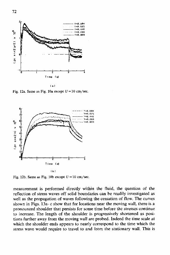
converted to the shear stress and the first normal stress difference as functions of time. The average velocity gradient corresponding to this flow condition (6.6 see-‘) is low enough so that the birefringence and first normal stress difference monotonically increase following the inception of flow. The shear stress, on the other hand, shows a pronounced overshoot. Figures 11 and 12 present the corresponding stress data for wall velocities of 7.5 and 10.0 cm/set, respectively. At these higher velocity gradients the first normal stress difference (and the birefringences, not shown here) overshoot. This phenomenon indicates that the chains overshoot in their deformation, or that there is a net decrease in entanglement junctions during the flow. Also, it is worth studying the response of the shear stress immediately following the cessation of flow. For the data acquired closest to the moving

69

------“-a.XB

n

6

4

2

0

Time (5)

(a)

Fig. 9a. Birefringence versus time for the inception and cessation of Couette flow for a 1.0 wt.% polyox solution, U = 5 cm/set.

45

10

5

0 0 I 2 3

Time (3

(b)

Fig. 9b. Orientation angle versus time for the inception and cessation of Couette flow for a 1.0 wt.% polyox solution, U = 5 cm/xc.

wall there is an undershoot in the shear stress and for the larger wall velocities, this undershoot actually causes the shear stress to change sign. This undershoot and sign reversal also occurs in the orientation angle and is due to the rapid deceleration of the flow near the moving wall as it comes to an abrupt stop. For large enough wall velocities there is a subsequent sign reversal in the velocity gradient near the moving wall.

The existence of wavelike propagation in the shear stress is shown when the data are plotted on shorter time scales as in Figs. 13a-c for wall

2

----- Y-0.904

.. Y=0.625

------ Y-0.446

Y-0.ZGE

-----Y-0.099

Time (set)

(a)

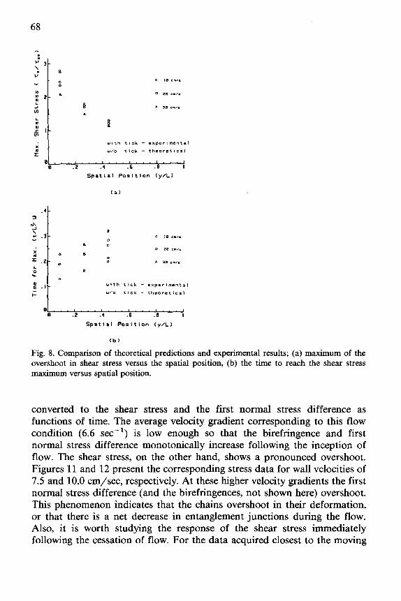
Fig. 10a. Shear stress versus time calculated from the data in Figs. 9a and 9b, U = 5 cm/xc.

Time (SC)

(b)

Fig. lob. First normal stress difference calculated from the data in Figs. 9a and 9b, lJ= 5 cm/set.

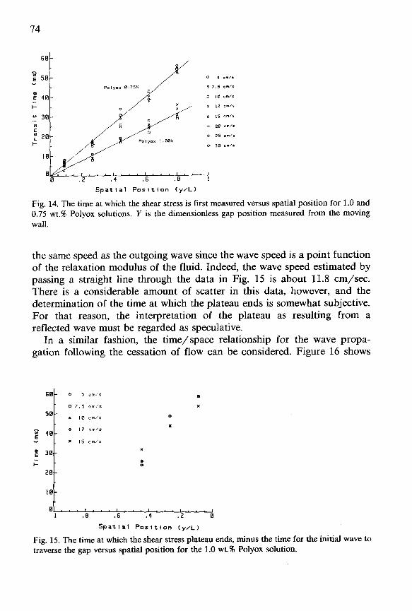
velocities of 5, 7.5 and 10 cm/set, respectively. The first important observa- tion is that the response at the early times is nearly independent of the wall velocity. In particular the times at which the stress first rises from zero scale linearly with the distance from the moving wall. This is brought out in Fig. 14 where plots of these times against spatial position produce straight lines that are independent of the wall velocity. The slope, of this line is the reciprocal of the wave speed that was calculated to be 18.2 cm/set. Similar data for a 0.75 wt.% poly(oxyethylene) solution is also plotted, yielding a

71

‘r

J__---_ I 2 3 4

Time (sl

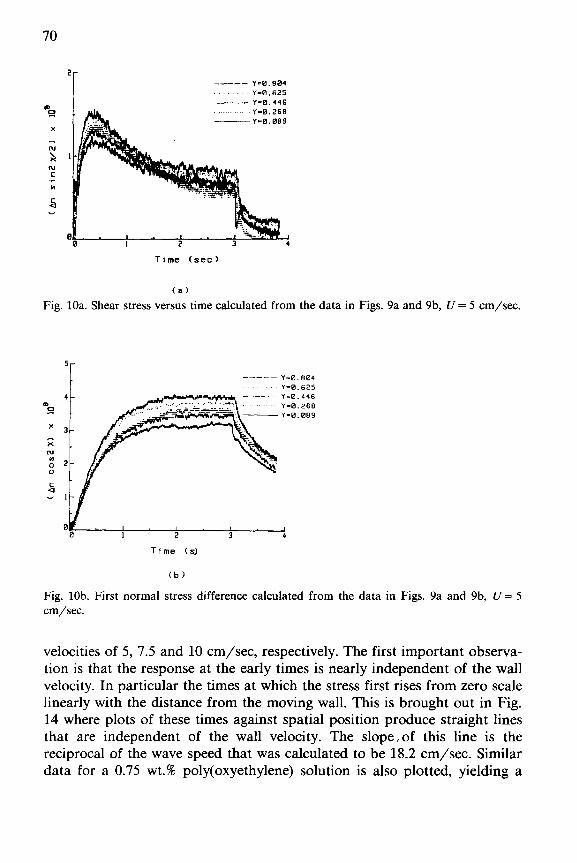
Fig. lla. Same as Fig. 10a except U= 7.5 cm/set.

e I 2 3 4

Time (~1

(b)

Fig. llb. Same as Fig. 10b except U= 7.5 cm/set.

wave speed of 10.8 cm/set. These values of the wave speed are in good agreement with those reported by Joseph, Riccius and Amey [12] using a “wave speed meter”. That device measured the time for an initial velocity disturbance to travel from the moving, outer wall of a Couette cell to the inner, stationary cylinder. This was done by measuring the mechanical response of the inner cylinder.

The use of flow birefringence as a means of investigating wave propa- gation phenomena has distinct advantages over mechanical methods that only respond to stresses at solid boundaries. Because the birefringence

72

-11 9 I I ,

a 1 2 3 4

Time (3

(a)

Fig. 12a. Same as Fig. 10a except U=lO cm/w.

0 ----- Y-0.804

7 ------ Y-0.446

4 6

x 5

2 q N

0” 3

; 2

I

0 a 1 2 3 4

Time (s)

(b)

Fig. 12b. Same as Fig. lob except U = 10 cm/set.

measurement is performed directly within the fluid, the question of the reflection of stress waves off solid boundaries can be readily investigated as well as the propagation of waves following the cessation of flow. The curves shown in Figs. 13a-c show that for locations near the moving wall, there is a pronounced shoulder that persists for some time before the stresses continue to increase. The length of the shoulder is progressively shortened as posi- tions further away from the moving wall are probed. Indeed the time scale at which the shoulder ends appears to nearly correspond to the time which the stress wave would require to travel to and from the stationary wall. This is

73

Time (3

I-

-.---- Y-0.904 y-0.929

------ Y-0.446 _.....,_....,... Y-0. 299

-Y-E. 089

Tcmc (s)

(a)

(b)

(cl

Fig. 13. The development of shear stress at early times; (a) U = 5 cm/xc, (b) U = 7.5 cm/set, (c) U = 10 cm/w.

brought out specifically in Fig. 15 where the times at which the plateau ends, minus the transit time for the initial wave to traverse the gap, are plotted against spatial position for various moving wall velocities. This is only possible for the three positions closest to the moving wall where the plateau is well defined. This observation and because these time scales are generally independent of the moving wall velocity suggest that the plateau may represent the dwell time between the first outgoing wave from the moving wall and the later, reflected wave from the stationary cylinder. It must be noted, however, that the reflected wave will not necessarily propagate with

74

60-

: 40- ._ k- -

+r 30- ._ w

fJ 20- ; _

I I I. * 1.8, 1. 3, 1, “1 0 .2 .4 .6 .E 1

Spatial Position (y/L)

Fig. 14. The time at which the shear stress is first measured versus spatial position for 1.0 and 0.75 wt.% Polyox solutions. Y is the dimensionless gap position measured from the moving wall.

the same speed as the outgoing wave since the wave speed is a point function of the relaxation modulus of the fluid. Indeed, the wave speed estimated by passing a straight line through the data in Fig. 15 is about 11.8 cm/set. There is a considerable amount of scatter in this data, however, and the determination of the time at which the plateau ends is somewhat subjective. For that reason, the interpretation of the plateau as resulting from a reflected wave must be regarded as speculative.

In a similar fashion, the time/space relationship for the wave propa- gation following the cessation of flow can be considered. Figure 16 shows

0l... I, * , I .*,I.,*,.,.,

1 .E .6 .4 .2 0

Spatial Position (y/L)

Fig. 15. The time at which the shear stress plateau ends, minus the time for the initial wave to traverse the gap versus spatial position for the 1.0 wt.% Polyox solution.

75

70c

Spatial Position (y/L)

Fig. 16. The time at which the shear stress fist decays during stress relaxation, minus the time at which the brake was applied versus spatial position.

the time for the shear stress to first decay from the steady shear value plotted against spatial position. Again, this plot yields a linear relationship but with slopes that depend on the moving wall velocity. In addition the slopes are higher and yield a corresponding slower wave speed than for the start-up of flow. A wave speed that decreases with velocity gradient is expected since the relaxation modulus is a decreasing function of shear rate. The measured wave speeds following the cessation of flow were found to be 13.9,11.8 and 9.9 cm/set for the 1.0 wt.% solution subjected to moving wall velocities of 5, 10 and 15 cm/set, respectively.

5. Conclusions

The spatial resolution of the flow birefringence measurement allows it to be used to interrogate inhomogeneous stress field. Furthermore, the polari- zation modulation method used here permits time-dependent flows to be studied. This combination of advantages makes this technique particularly well suited to the Rayleigh problem where the stress field varies in both space and time.

The measurements made using the Newtonian polybutene liquid showed that the technique is capable of accurate determinations of stress and the results agreed well with the exact solutions that are available for this type of fluid. In principle, wave propagation phenomena could occur with this liquid at short times but the time scale required to start the flow (approxi- mately 20 ms) is most likely too long for the large wave speeds that would be expected for this grade of polybutene. This shortcoming is associated with the particular mechanism used to initiate flow (the electromagnetic clutch)

76

and not the method used to measure the birefringence. The polymer solu- tions studied here, on the other hand, offer sufficiently slow wave speeds that evidence for the existence of shear waves was readily apparent. Waves were observed to not only propagate at the inception of flow but also following stoppage of the flow and off solid boundaries during start-up.

Acknowledgement

This research was sponsored by the National Science Foundation under the Presidential Young Investigator Award CPT-8451446.

References

1 H. Schhchting, Boundary Layer Theory, McGraw-Hill, NY, 1979, 90-92,168-173. pp. 2 G.K. Batchelor, An Introduction to Fluid Dynamics, Cambridge University Press, Cam-

bridge, 1980, pp. 189-193. 3 T.Y. Kazakia and R.S. Rivlin, Rheol. Acta, 20 (1981) 111. 4 R.I. Tanner, ZAMP, 13 (1962) 573. 5 D.D. Joseph and J.C. Saut, J. Non-Newtonian Fluid Mech., 20 (1986) 117. 6 A. Narain and D.D. Joseph, Rheol. Acta, /fl21, (1982) 228. 7 Y. Mochimaru, J. Non-Newtonian Fluid Mech., 12 (1983) 135. 8 H. Janeschitz-KriegI, Adv. Polym. Sci., 6 (1969) 170. 9 A.W. Chow, G.G. Fuller, D.G. Wallace and J.A. Madri, Macromolecules, 18 (1985) 793.

10 S.J. Johnson, P.L. Frattini and G.G. Fuller, J. Coll. Inter. Sci., 104, (1985) 440. 11 V.N. Tsvetkov, Soviet Phys. Uspekhi, 6 (1964) 639. 12 D.D. Joseph, 0. Riccius and M. Arney, J. Fluid Mech., 171 (1986) 309. 13 J.S. Lee, Engineer’s Thesis, Stanford University, California, 1987.