The Solar Neighborhood. XXXIX. Parallax Results from the CTIOPI and NOFSPrograms: 50 New Members of the 25 parsec White Dwarf Sample

John P. Subasavage1,8, Wei-Chun Jao2,8, Todd J. Henry3,8, Hugh C. Harris1, Conard C. Dahn1, P. Bergeron4, P. Dufour4,Bart H. Dunlap5, Brad N. Barlow6, Philip A. Ianna3,8, Sébastien Lépine2, and Steven J. Margheim7

1 U.S. Naval Observatory, 10391 West Naval Observatory Road, Flagstaff, AZ 86005-8521, USA; jsubasavage@nofs.navy.mil2 Department of Physics and Astronomy, Georgia State University, Atlanta, GA 30302-4106, USA

3 RECONS Institute, Chambersburg, PA 17201, USA4 Département de Physique, Université de Montréal, C.P. 6128, Succ. Centre-Ville, Montréal, Québec H3C 3J7, Canada

5 University of North Carolina at Chapel Hill, Dept. of Physics and Astronomy, Chapel Hill, NC 27599, USA6 Department of Physics, High Point University, One University Parkway, High Point, NC 27268, USA

7 Gemini Observatory, Southern Operations Center, Casilla 603, La Serena, ChileReceived 2017 March 21; revised 2017 May 31; accepted 2017 May 31; published 2017 June 30

Abstract

We present 114 trigonometric parallaxes for 107 nearby white dwarf (WD) systems from both the Cerro TololoInter-American Observatory Parallax Investigation (CTIOPI) and the U.S.Naval Observatory Flagstaff Station(NOFS) parallax programs. Of these, 76 parallaxes for 69 systems were measured by the CTIOPI program and 38parallaxes for as many systems were measured by the NOFS program. A total of 50 systems are confirmed to bewithin the25-pc horizon of interest. Coupled with a spectroscopic confirmation of a common proper-motioncompanion to a Hipparcos star within 25 pc as well as confirmation parallax determinations for two WD systemsincluded in the recently released Tycho Gaia Astrometric Solution catalog, we add 53 new systems to the 25-pcWD sample—a 42% increase. Our sample presented here includes four strong candidate halo systems, a newmetal-rich DAZ WD, a confirmation of a recently discovered nearby short-period (P=2.85 hr) double degenerate,a WD with a new astrometric perturbation (long period, unconstrained with our data), and a new triple systemwhere the WD companion main-sequence star has an astrometric perturbation (P∼1.6 year).

Key words: astrometry – Galaxy: evolution – solar neighborhood – stars: distances – white dwarfs

Supporting material: data behind figures, machine-readable tables

1. Introduction

White dwarfs (WDs) are the remarkably abundant remnants ofthe vast majority of stars and serve as reliable tracers for a numberof astrophysically interesting topics. We aim to compile a robust,volume-limited sample of WDs upon which statistical studies canbe performed. For instance, insight into population membershippercentages (thin disk, thick disk, halo), population ages, andGalactic star formation history can be ascertained from the sampleas a whole. Individually, a non-trivial number of WDs are foundto be metal-enriched and are most likely displaying signs ofdisrupted planetary systems (Farihi et al. 2009and referencetherein). Given that the nearest metal-enriched WDs are thebrightest examples, they can be more carefully studied. With avolume-limited sample, one minimizes biases in the WDluminosity function, mass function, and those introduced wheninferring the number of planetary systems around WDs.

We present here a compilation of two long-term astrometricefforts to measure accurate trigonometric parallaxes to nearbyWDs—the Cerro Tololo Inter-American Observatory ParallaxInvestigation (CTIOPI, Jao et al. 2005) and the U.S.NavalObservatory Flagstaff Station (NOFS, Monet et al. 1992) parallaxprogram. In total, 76 parallaxes are measured for 69 systems bythe CTIOPI program and 38 parallaxes are measured for as manysystems by the NOFS program, including seven systems forwhich both CTIOPI and NOFS measured parallaxes. The CTIOPI

results represent all completed parallaxes for WDs on theprogram, including those beyond the 25-pc horizon of interest.A subset of the CTIOPI targets are members of the 15 pcAstrometric Search for Planets Encircling Nearby Stars (ASPENS,Koerner et al. 2003) initiative. These targets typically have ∼10+years of data and will be continually monitored as long as theprogram will allow. The NOFS parallaxes only include thosewithin the 25-pc horizon of interest. A much larger sample of WDparallaxes from NOFS at all distances will be included inaforthcoming publication.The combined astrometric efforts add 50 WD systems to the

25-pc sample (27 from CTIOPI, 20 from NOFS, and 3 measuredby both programs). Also, we spectroscopically confirmed apreviously unknown WD companion to a main-sequence dwarfwith a Hipparcos parallax placing the system within 25 pc.Finally, we confirm proximity for two WDs whose trigonometricparallaxes were also recently determined by the Tycho Gaiaastrometric solution (TGAS, Lindegren et al. 2016). Thus, a totalof 53 new systems are added to the 25-pc WD sample thatpreviously consisted of 126 systems reliably within that volume—a 42% increase. The complete sample of WDs within 25 pc can befound at http://www.DenseProject.com.

2. Observations and Data

2.1. Photometry

2.1.1. Optical BVRI Photometry

Standardized photometric observations were carried out atthree separate telescopes. The SMARTS 0.9 m telescope at

The Astronomical Journal, 154:32 (24pp), 2017 July https://doi.org/10.3847/1538-3881/aa76e0© 2017. The American Astronomical Society. All rights reserved.

8 Visiting astronomer, Cerro Tololo Inter-American Observatory, NationalOptical Astronomy Observatory, which are operated by the Association ofUniversities for Research in Astronomy, under contract with the NationalScience Foundation.

1

CTIO was used during CTIOPI observing runs when condi-tions were photometric. A Tektronics 2 K×2 K detector wasused in region-of-interest mode centered on the central quarterof the full CCD producing a field of view (FOV) of 6 8×6 8.The SMARTS 1.0 m telescope at CTIO was used with theY4KCam 4 K×4 K imager, producing a 19 7×19 7 FOV.Finally, the Ritchey 40-in telescope at USNO Flagstaff Stationwas used with a Tektronics 2 K×2 K detector with a20 0×20 0 FOV. Calibration frames (biases, dome and/orsky flats) were taken nightly and were used to perform basiccalibrations of the science data using standard IRAF packages.Standard stars from Graham (1982) and Landolt(1992, 2007, 2013) were taken nightly through a range ofairmasses to calibrate fluxes to the Johnson–Kron–Cousinssystem and to calculate extinction corrections. In general,aperture photometry was performed on both standard stars andtarget stars using a 14″ diameter. For crowded fields, fainttargets, and recent observations, once a PSF pipeline was inplace, PSF photometry was conducted using either theDAOPhot (Stetson 1987) or the PSFEx (Bertin 2011)algorithm. A subset of data were compared using both PSFalgorithms and no significant systematic offset was seen. Whilethree separate Johnson–Kron–Cousins VRI filter sets were usedbetween the three telescopes, comparisons were made ofdozens of CTIOPI targets mutually observed with all filter sets.Any systematic variation inherent in the filter set differencesonce standardized is well below our nominal magnitude errorof 0.03 mag.

For the CTIOPI program, relative brightnesses were alsorecorded for the parallax target (hereafter referred to as the “PI”star) compared to the astrometric reference field stars in thefilter used for the astrometry as part of the CTIOPI reductionpipeline. From these data, we gauge whether the PI star showsany variability. If any of the reference stars show variabilityabove ∼2%, they are removed from the variability analysis.This analysis was not performed for the NOFS targets as it wasnot part of the reduction pipeline. Photometry values are givenin Table 1, where columns (1) and (2) give WD and alternatenames, respectively. Columns (3)–(10) give the Johnson BV,Kron-Cousins RI, and corresponding number of observations ineach filter. Columns (11)–(14) give the filter of parallaxobservations (hereafter referred to as the parallax filter) and PIstar photometric standard deviation in that filter as a gauge forvariability as well as the number of nights and frames used forthe variability analysis. Columns (15)–(17) give the JHKs

photometry values and corresponding errors on the 2MASSphotometric system. Finally, column (18) contains any notes.

2.1.2. NOAO Extremely Wide-field InfraredImager (NEWFIRM) JHK Photometry

Near-IR JHKs photometry was collected for WD 0851−246,at the CTIO 4.0 m Blanco telescope using the NEWFIRM(Probst et al. 2004) during an engineering night on 2011.27UT. NEWFIRM is a 4 K×4 K InSb mosaic that provides a28′×28′FOV on the Blanco telescope. Raw data wereprocessed using the NEWFIRM science reduction pipelineand retrieved from the NOAO science archive as fullyprocessed, stacked images.

Relative photometry was performed using the 2MASScatalog to standardize the images. Frames were checked toidentify where saturation occurs and comparison stars wereselected to have high signal-to-noise yet below saturation. A

total of 68 comparison stars were used for each frame with2MASS magnitudes ranging from 12.61 to 14.42, 12.24 to13.99, and 12.14 to 13.90 for J, H, and Ks, respectively. TheNEWFIRM filters are on the MKO system so the comparisonstars were transformed to the MKO system using themethodology of Carpenter (2001).9 Instrumental PSF photo-metry was extracted using PSFEx for the comparison stars andthe target. A least-squares fit was used to determine the offsetbetween instrumental J and MKO J. A similar approach wasused to determine the MKO J−H and J−K colors.Photometry values and errors are listed in Table 1 and areitalicized to distinguish them from other JHKs values on the2MASS photometric system.

2.1.3. Catalog Photometry

Additional photometry values were extracted from the SloanDigital Sky Survey (SDSS) DR12 (Alam et al. 2015), 2MASS,and the UKIRT Infrared Sky Survey (UKIDSS) DR9 LargeArea Survey, when available. The UKIDSS project is outlinedin Lawrence et al. (2007). UKIDSS uses the UKIRT WideField Camera (Casali et al. 2007). The photometric systemis described in Hewett et al. (2006)and the calibration isdescribed in Hodgkin et al. (2009). The science archive isdescribed in Hambly et al. (2008). UKIDSS magnitudes weretransformed to the 2MASS system using the transformations ofHodgkin et al. (2009). These transformed values are listed inTable 1. We do not tabulate the photometry extracted fromSDSS DR12 as those are readily available via the SDSSarchive.

2.2. Spectroscopy

Two WDs presented here (WD 1743−545 and WD 2057−493) are newly discovered nearby WDs identified during aspectroscopic survey of WD candidates in the southernhemisphere (J. Subasavage et al. 2017, in preparation) takenfrom the SUPERBLINK catalog (Lépine & Shara 2005). Athird WD included here (WD 2307−691) was previouslyunclassified, yet is a common proper-motion companion to aHipparcos star within 25 pc (HIP 114416). A fourth WD (WD2028−171) was suspected to be a WD by the authors based ona trawl of the New Luyten Two Tenths (NLTT) catalog (Luyten1979a). Finally, afifth WD (WD 1241−798) was firstspectroscopically identified as a WD by Subasavage et al.(2008) but with an ambiguous spectral type of DC/DQ. TheSOAR 4 m telescope with the Goodman spectrograph was usedfor spectroscopic follow up as part of a larger spectroscopiccampaign to identify nearby WDs to be released in a futurepublication. Observations were taken with a 600 lines-per-mmVPH grating with a 1 0 slit width to provide 2.1 Åresolutionin wavelength range of 3600 Å−6200 Å. The slit was rotated tothe parallactic angle to prevent any color-differential loss oflight. For WD 1241−798, the spectrum was taken during anengineering night and only quartz lamp flats were taken. Theundulations seen in the spectrum correlate with thestructure ofthe quartz lamp and thusarenot real. For these spectra andthroughout this work, we adopt the WD spectral classificationsystem of Sion et al. (1983). In brief, DA WDs contain Balmerfeatures, DB WDs contain helium features, DC WDs are

9 The MKO transformations were not included in Carpenter (2001) but wereadded later and areavailable at http://www.astro.caltech.edu/~jmc/2mass/v3/transformations/.

2

The Astronomical Journal, 154:32 (24pp), 2017 July Subasavage et al.

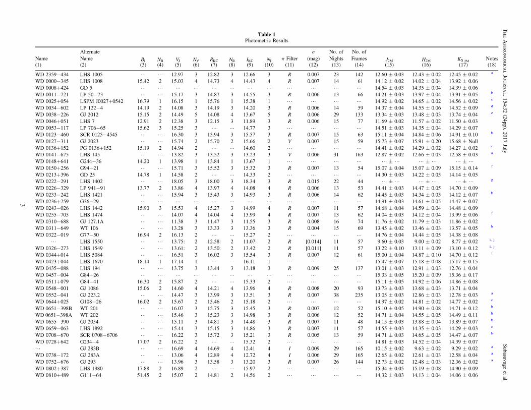
Table 1Photometric Results

Alternate σ No. of No. ofName Name BJ NB VJ NV RKC NR IKC NI π Filter (mag) Nights Frames J2M H2M KS 2M Notes(1) (2) (3) (4) (5) (6) (7) (8) (9) (10) (11) (12) (13) (14) (15) (16) (17) (18)

WD 2359−434 LHS 1005 L L 12.97 3 12.82 3 12.66 3 R 0.007 23 142 12.60±0.03 12.43±0.02 12.45±0.02 a

WD 0000−345 LHS 1008 15.42 2 15.03 4 14.73 4 14.43 4 R 0.007 14 61 14.12±0.02 14.02±0.04 13.92±0.06WD 0008+424 GD 5 L L L L L L L L L L L L 14.54±0.03 14.35±0.04 14.39±0.06WD 0011−721 LP 50−73 L L 15.17 3 14.87 3 14.55 3 R 0.006 13 66 14.21±0.03 13.97±0.04 13.91±0.05 b

WD 0025+054 LSPM J0027+0542 16.79 1 16.15 1 15.76 1 15.38 1 L L L L 14.92±0.02 14.65±0.02 14.56±0.02 c

WD 0034−602 LP 122−4 14.19 2 14.08 3 14.19 3 14.20 3 R 0.006 14 59 14.37±0.04 14.55±0.06 14.52±0.09 d

WD 0038−226 GJ 2012 15.15 2 14.49 5 14.08 4 13.67 5 R 0.006 29 133 13.34±0.03 13.48±0.03 13.74±0.04 e

WD 0046+051 LHS 7 12.91 2 12.38 3 12.15 3 11.89 3 R 0.006 15 77 11.69±0.02 11.57±0.02 11.50±0.03WD 0053−117 LP 706−65 15.62 3 15.25 3 L L 14.77 3 L L L L 14.51±0.03 14.35±0.04 14.29±0.07WD 0123−460 SCR 0125−4545 L L 16.30 3 15.94 3 15.57 3 R 0.007 15 63 15.11±0.04 14.84±0.06 14.91±0.10 b

WD 0127−311 GJ 2023 L L 15.74 2 15.70 2 15.66 2 V 0.007 15 59 15.73±0.07 15.91±0.20 15.68±NullWD 0136+152 PG 0136+152 15.19 2 14.94 2 L L 14.60 2 L L L L 14.41±0.02 14.29±0.02 14.27±0.02 c

WD 0141−675 LHS 145 L L 13.82 3 13.52 3 13.23 3 V 0.006 31 163 12.87±0.02 12.66±0.03 12.58±0.03 a

WD 0148+641 G244−36 14.20 1 13.98 1 13.84 1 13.67 1 L L L L L±L L±L L±LWD 0150+256 G94−21 L L 15.71 3 15.52 3 15.32 3 R 0.007 13 54 15.07±0.04 15.07±0.09 15.15±0.14 f

WD 0213+396 GD 25 14.78 1 14.58 2 L L 14.33 2 L L L L 14.30±0.03 14.22±0.05 14.14±0.05WD 0222−291 LHS 1402 L L 18.05 3 18.00 3 18.34 3 R 0.015 22 44 L±L L±L L±L g

WD 0226−329 LP 941−91 13.77 2 13.86 4 13.97 4 14.08 4 R 0.006 13 53 14.41±0.03 14.47±0.05 14.70±0.09WD 0233−242 LHS 1421 L L 15.94 3 15.43 3 14.93 3 R 0.006 14 62 14.45±0.03 14.34±0.05 14.12±0.07 b

WD 0236+259 G36−29 L L L L L L L L L L L L 14.91±0.03 14.61±0.05 14.47±0.07WD 0243−026 LHS 1442 15.90 3 15.53 4 15.27 3 14.99 4 R 0.007 11 57 14.68±0.04 14.59±0.04 14.48±0.09WD 0255−705 LHS 1474 L L 14.07 4 14.04 4 13.99 4 R 0.007 13 62 14.04±0.03 14.12±0.04 13.99±0.06 f

WD 0310−688 GJ 127.1A L L 11.38 3 11.47 3 11.55 3 R 0.008 16 74 11.76±0.02 11.79±0.03 11.86±0.02WD 0311−649 WT 106 L L 13.28 3 13.33 3 13.36 3 R 0.004 15 69 13.45±0.02 13.46±0.03 13.57±0.05 h

WD 0322−019 G77−50 16.94 2 16.13 2 L L 15.27 2 L L L L 14.76±0.04 14.44±0.05 14.38±0.08L LHS 1550 L L 13.75: 2 12.58: 2 11.07: 2 R [0.014] 11 57 9.60±0.03 9.00±0.02 8.77±0.02 i, j

WD 0326−273 LHS 1549 L L 13.61: 2 13.50: 2 13.42: 2 R [0.011] 11 57 13.22±0.10 13.11±0.09 13.10±0.12 i, j

WD 0344+014 LHS 5084 L L 16.51 3 16.02 3 15.54 3 R 0.007 12 61 15.00±0.04 14.87±0.10 14.70±0.12 f

WD 0423+044 LHS 1670 18.14 1 17.14 1 L L 16.11 1 L L L L 15.47±0.07 15.18±0.08 15.17±0.15WD 0435−088 LHS 194 L L 13.75 3 13.44 3 13.18 3 R 0.009 25 137 13.01±0.03 12.91±0.03 12.76±0.04WD 0457−004 G84−26 L L L L L L L L L L L L 15.33±0.05 15.20±0.09 15.36±0.17WD 0511+079 G84−41 16.30 2 15.87 2 L L 15.33 2 L L L L 15.11±0.05 14.92±0.06 14.86±0.08WD 0548−001 GJ 1086 15.06 2 14.60 4 14.21 4 13.96 4 R 0.008 20 93 13.73±0.03 13.68±0.03 13.71±0.04WD 0552−041 GJ 223.2 L L 14.47 3 13.99 3 13.51 3 R 0.007 38 235 13.05±0.03 12.86±0.03 12.78±0.03 a

WD 0644+025 G108−26 16.02 2 15.67 2 15.46 2 15.18 2 L L L L 14.97±0.02 14.81±0.02 14.77±0.02 c

WD 0651−398B WT 201 L L 16.07 3 15.75 3 15.45 3 R 0.007 12 52 15.10±0.05 14.90±0.08 14.71±0.12 h

WD 0651−398A WT 202 L L 15.46 3 15.23 3 14.98 3 R 0.006 12 52 14.71±0.04 14.55±0.05 14.49±0.11 h

WD 0655−390 GJ 2054 L L 15.11 3 14.81 3 14.48 3 R 0.007 11 48 14.15±0.03 13.88±0.04 13.89±0.07 b

WD 0659−063 LHS 1892 L L 15.44 3 15.15 3 14.86 3 R 0.007 11 57 14.55±0.03 14.35±0.03 14.29±0.03 c

WD 0708−670 SCR 0708−6706 L L 16.22 3 15.72 3 15.21 3 R 0.005 13 59 14.71±0.03 14.65±0.05 14.47±0.07 b

WD 0728+642 G234−4 17.07 2 16.22 2 L L 15.32 2 L L L L 14.81±0.03 14.52±0.04 14.39±0.07L GJ 283B L L 16.69 4 14.69 4 12.41 4 I 0.009 29 165 10.15±0.02 9.63±0.02 9.29±0.02 a

WD 0738−172 GJ 283A L L 13.06 4 12.89 4 12.72 4 I 0.006 29 165 12.65±0.02 12.61±0.03 12.58±0.04 a

WD 0752−676 GJ 293 L L 13.96 3 13.58 3 13.20 3 R 0.007 26 144 12.73±0.02 12.48±0.03 12.36±0.02 a

WD 0802+387 LHS 1980 17.88 2 16.89 2 L L 15.97 2 L L L L 15.34±0.05 15.19±0.08 14.90±0.09WD 0810+489 G111−64 51.45 2 15.07 2 14.81 2 14.56 2 L L L L 14.32±0.03 14.13±0.04 14.06±0.06

3

TheAstro

nomica

lJourn

al,

154:32(24pp),

2017July

Subasavage

etal.

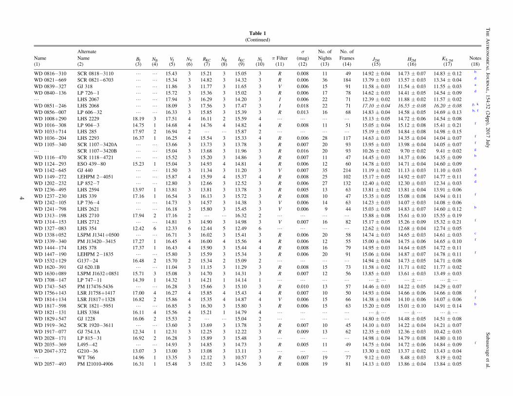
Table 1(Continued)

Alternate σ No. of No. ofName Name BJ NB VJ NV RKC NR IKC NI π Filter (mag) Nights Frames J2M H2M KS 2M Notes(1) (2) (3) (4) (5) (6) (7) (8) (9) (10) (11) (12) (13) (14) (15) (16) (17) (18)

WD 0816−310 SCR 0818−3110 L L 15.43 3 15.21 3 15.05 3 R 0.008 11 49 14.92±0.04 14.73±0.07 14.83±0.12 b

WD 0821−669 SCR 0821−6703 L L 15.34 3 14.82 3 14.32 3 R 0.006 36 184 13.79±0.03 13.57±0.03 13.34±0.04 d

WD 0839−327 GJ 318 L L 11.86 3 11.77 3 11.65 3 V 0.006 15 91 11.58±0.03 11.54±0.03 11.55±0.03 a

WD 0840−136 LP 726−1 L L 15.72 3 15.36 3 15.02 3 R 0.006 17 78 14.62±0.03 14.41±0.05 14.54±0.09 d

L LHS 2067 L L 17.94 3 16.29 3 14.20 3 I 0.006 22 71 12.39±0.02 11.88±0.02 11.57±0.02WD 0851−246 LHS 2068 L L 18.09 3 17.56 3 17.47 3 I 0.018 22 71 17.10±0.04 16.55±0.08 16.20±0.08 g, k

WD 0856−007 LP 606−32 L L 16.33 3 15.85 3 15.39 3 R 0.013 16 68 14.83±0.04 14.58±0.05 14.69±0.13 b, f

WD 1008+290 LHS 2229 18.19 3 17.51 4 16.11 2 15.59 4 L L L L 15.13±0.05 14.72±0.06 14.54±0.08WD 1016−308 LP 904−3 14.75 1 14.68 4 14.76 4 14.82 4 R 0.008 11 51 15.05±0.04 15.12±0.08 15.41±0.21 f

WD 1033+714 LHS 285 17.97 2 16.94 2 L L 15.87 2 L L L L 15.19±0.05 14.84±0.08 14.98±0.15WD 1036−204 LHS 2293 16.37 1 16.25 4 15.54 3 15.33 4 R 0.006 28 117 14.63±0.03 14.35±0.04 14.04±0.07 f

WD 1105−340 SCR 1107−3420A L L 13.66 3 13.73 3 13.78 3 R 0.007 20 93 13.95±0.03 13.98±0.04 14.05±0.07 f

L SCR 1107−3420B L L 15.04 3 13.68 3 11.96 3 R 0.016 20 93 10.26±0.02 9.70±0.02 9.41±0.02 g

WD 1116−470 SCR 1118−4721 L L 15.52 3 15.20 3 14.86 3 R 0.007 11 47 14.45±0.03 14.37±0.06 14.35±0.09 b

WD 1124−293 ESO 439−80 15.23 1 15.04 3 14.93 4 14.81 4 R 0.006 12 60 14.78±0.03 14.71±0.04 14.60±0.09WD 1142−645 GJ 440 L L 11.50 3 11.34 3 11.20 3 V 0.007 35 214 11.19±0.02 11.13±0.03 11.10±0.03 a

WD 1149−272 LEHPM 2−4051 L L 15.87 4 15.59 4 15.37 4 R 0.008 25 102 15.17±0.05 14.92±0.07 14.77±0.11 d

WD 1202−232 LP 852−7 L L 12.80 3 12.66 3 12.52 3 R 0.006 27 132 12.40±0.02 12.30±0.03 12.34±0.03 d

WD 1236−495 LHS 2594 13.97 1 13.81 3 13.81 3 13.78 3 R 0.005 13 63 13.81±0.02 13.81±0.04 13.91±0.06WD 1237−230 LHS 339 17.16 1 16.54 3 16.13 3 15.72 3 R 0.008 10 47 15.35±0.05 15.08±0.08 14.94±0.11 f

WD 1242−105 LP 736−4 L L 14.73 3 14.57 3 14.38 3 V 0.006 14 63 14.23±0.03 14.07±0.03 14.08±0.06WD 1241−798 LHS 2621 L L 16.18 3 15.80 3 15.45 3 V 0.006 9 44 15.03±0.05 14.83±0.07 14.60±0.12 b

WD 1313−198 LHS 2710 17.94 2 17.16 2 L L 16.32 2 L L L L 15.88±0.08 15.61±0.10 15.55±0.19WD 1314−153 LHS 2712 L L 14.81 3 14.90 3 14.98 3 V 0.007 16 82 15.17±0.05 15.26±0.09 15.32±0.21 f

WD 1327−083 LHS 354 12.42 6 12.33 6 12.44 5 12.49 6 L L L L 12.62±0.04 12.68±0.04 12.74±0.05WD 1338+052 LSPM J1341+0500 L L 16.71 3 16.02 3 15.41 3 R 0.006 20 58 14.74±0.03 14.65±0.03 14.61±0.03 c

WD 1339−340 PM J13420−3415 17.27 1 16.45 4 16.00 4 15.56 4 R 0.006 12 55 15.00±0.04 14.75±0.06 14.65±0.10 f

WD 1444−174 LHS 378 17.37 1 16.43 4 15.90 3 15.44 4 R 0.008 16 79 14.95±0.03 14.64±0.05 14.72±0.11WD 1447−190 LEHPM 2−1835 L L 15.80 3 15.59 3 15.34 3 R 0.006 20 91 15.06±0.04 14.87±0.07 14.78±0.11 f

WD 1532+129 G137−24 16.48 2 15.70 2 15.34 2 15.09 2 L L L L 14.94±0.04 14.73±0.05 14.71±0.08WD 1620−391 GJ 620.1B L L 11.04 3 11.15 3 11.29 3 R 0.008 15 73 11.58±0.02 11.71±0.02 11.77±0.02WD 1630+089 LSPM J1632+0851 15.71 3 15.08 3 14.70 3 14.31 3 R 0.007 12 56 13.85±0.03 13.61±0.03 13.49±0.03WD 1708−147 LP 747−11 14.39 1 14.32 1 14.21 1 14.14 1 L L L L L±L L±L L±LWD 1743−545 PM I17476-5436 L L 16.28 3 15.66 3 15.10 3 R 0.010 13 57 14.46±0.03 14.22±0.05 14.29±0.07WD 1756+143 LSR J1758+1417 17.00 4 16.27 4 15.85 4 15.43 4 R 0.007 10 50 14.93±0.04 14.66±0.06 14.66±0.08 f

WD 1814+134 LSR J1817+1328 16.82 2 15.86 4 15.35 4 14.87 4 V 0.006 15 66 14.38±0.04 14.10±0.06 14.07±0.06 f

WD 1817−598 SCR 1821−5951 L L 16.85 3 16.30 3 15.80 3 R 0.006 15 63 15.20±0.05 15.01±0.10 14.91±0.14 b

WD 1821−131 LHS 3384 16.11 4 15.56 4 15.21 1 14.79 4 L L L L L±L L±L L±LWD 1829+547 GJ 1228 16.06 2 15.53 2 L L 15.04 2 L L L L 14.80±0.05 14.48±0.05 14.51±0.08WD 1919−362 SCR 1920−3611 L L 13.60 3 13.69 3 13.78 3 R 0.007 10 45 14.10±0.03 14.22±0.04 14.21±0.07WD 1917−077 GJ 754.1A 12.34 1 12.31 3 12.25 3 12.22 3 R 0.009 13 62 12.35±0.03 12.36±0.03 10.42±0.03WD 2028−171 LP 815−31 16.92 2 16.28 3 15.89 3 15.48 3 L L L L 14.98±0.04 14.79±0.08 14.80±0.10WD 2035−369 L495−42 L L 14.93 3 14.85 3 14.73 3 R 0.005 11 49 14.75±0.04 14.72±0.06 14.84±0.09 f

WD 2047+372 G210−36 13.07 3 13.00 3 13.08 3 13.11 3 L L L L 13.30±0.02 13.37±0.02 13.43±0.04L WT 766 14.96 1 13.35 3 12.12 3 10.57 3 R 0.007 19 77 9.12±0.03 8.48±0.03 8.19±0.02WD 2057−493 PM I21010-4906 16.31 1 15.48 3 15.02 3 14.56 3 R 0.008 19 81 14.13±0.03 13.86±0.04 13.84±0.05

4

TheAstro

nomica

lJourn

al,

154:32(24pp),

2017July

Subasavage

etal.

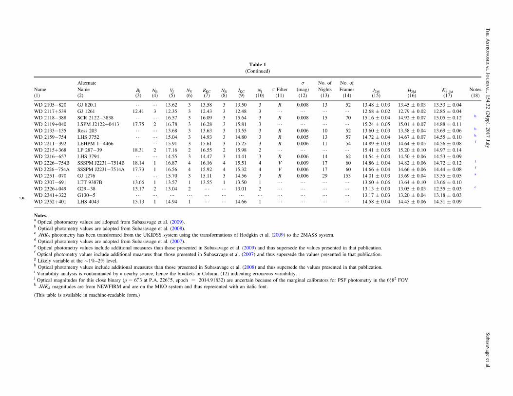
Table 1(Continued)

Alternate σ No. of No. ofName Name BJ NB VJ NV RKC NR IKC NI π Filter (mag) Nights Frames J2M H2M KS 2M Notes(1) (2) (3) (4) (5) (6) (7) (8) (9) (10) (11) (12) (13) (14) (15) (16) (17) (18)

WD 2105−820 GJ 820.1 L L 13.62 3 13.58 3 13.50 3 R 0.008 13 52 13.48±0.03 13.45±0.03 13.53±0.04WD 2117+539 GJ 1261 12.41 3 12.35 3 12.43 3 12.48 3 L L L L 12.68±0.02 12.79±0.02 12.85±0.04WD 2118−388 SCR 2122−3838 L L 16.57 3 16.09 3 15.64 3 R 0.008 15 70 15.16±0.04 14.92±0.07 15.05±0.12 h

WD 2119+040 LSPM J2122+0413 17.75 2 16.78 3 16.28 3 15.81 3 L L L L 15.24±0.05 15.01±0.07 14.88±0.11WD 2133−135 Ross 203 L L 13.68 3 13.63 3 13.55 3 R 0.006 10 52 13.60±0.03 13.58±0.04 13.69±0.06 b

WD 2159−754 LHS 3752 L L 15.04 3 14.93 3 14.80 3 R 0.005 13 57 14.72±0.04 14.67±0.07 14.55±0.10 h

WD 2211−392 LEHPM 1−4466 L L 15.91 3 15.61 3 15.25 3 R 0.006 11 54 14.89±0.03 14.64±0.05 14.56±0.08 f

WD 2215+368 LP 287−39 18.31 2 17.16 2 16.55 2 15.98 2 L L L L 15.41±0.05 15.20±0.10 14.97±0.14WD 2216−657 LHS 3794 L L 14.55 3 14.47 3 14.41 3 R 0.006 14 62 14.54±0.04 14.50±0.06 14.53±0.09WD 2226−754B SSSPM J2231−7514B 18.14 1 16.87 4 16.16 4 15.51 4 V 0.009 17 60 14.86±0.04 14.82±0.06 14.72±0.12 f

WD 2226−754A SSSPM J2231−7514A 17.73 1 16.56 4 15.92 4 15.32 4 V 0.006 17 60 14.66±0.04 14.66±0.06 14.44±0.08 f

WD 2251−070 GJ 1276 L L 15.70 3 15.11 3 14.56 3 R 0.006 29 153 14.01±0.03 13.69±0.04 13.55±0.05 a

WD 2307−691 LTT 9387B 13.66 1 13.57 1 13.55 1 13.50 1 L L L L 13.60±0.06 13.64±0.10 13.66±0.10WD 2326+049 G29−38 13.17 2 13.04 2 L L 13.01 2 L L L L 13.13±0.03 13.05±0.03 12.55±0.03 c

WD 2341+322 G130−5 L L L L L L L L L L L L 13.17±0.03 13.20±0.04 13.18±0.03WD 2352+401 LHS 4043 15.13 1 14.94 1 L L 14.66 1 L L L L 14.58±0.04 14.45±0.06 14.51±0.09

Notes.a Optical photometry values are adopted from Subasavage et al. (2009).b Optical photometry values are adopted from Subasavage et al. (2008).c JHKS photometry has been transformed from the UKIDSS system using the transformations of Hodgkin et al. (2009) to the 2MASS system.d Optical photometry values are adopted from Subasavage et al. (2007).e Optical photometry values include additional measures than those presented in Subasavage et al. (2009) andthus supersede the values presented in that publication.f Optical photometry values include additional measures than those presented in Subasavage et al. (2007) and thus supersede the values presented in that publication.g Likely variable at the ∼1%–2% level.h Optical photometry values include additional measures than those presented in Subasavage et al. (2008) andthus supersede the values presented in that publication.i Variability analysis is contaminated by a nearby source, hence the brackets in Column (12) indicating erroneous variability.j Optical magnitudes for this close binary (r = 6. 3 at P.A. 226 . 5, epoch = 2014.91832) are uncertain because of the marginal calibrators for PSF photometry in the 6 82 FOV.k JHKS magnitudes are from NEWFIRM and are on the MKO system and thus represented with an italic font.

(This table is available in machine-readable form.)

5

TheAstro

nomica

lJourn

al,

154:32(24pp),

2017July

Subasavage

etal.

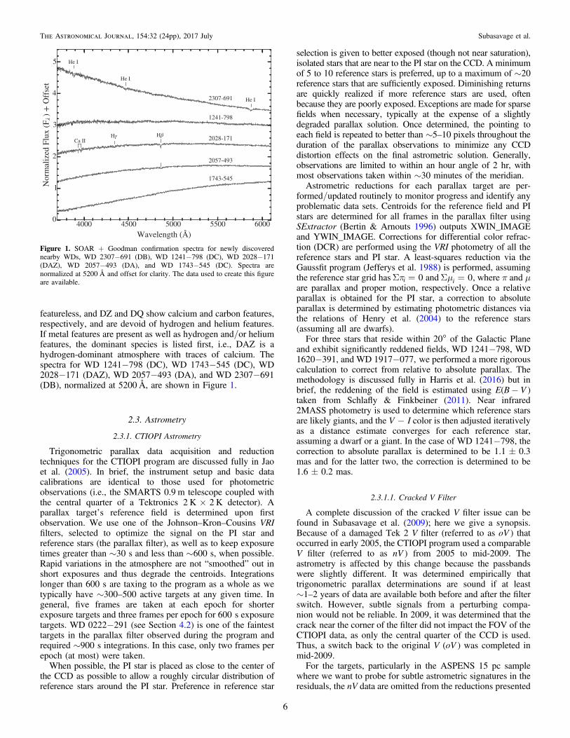
featureless, and DZ and DQ show calcium and carbon features,respectively, and are devoid of hydrogen and helium features.If metal features are present as well as hydrogen and/or heliumfeatures, the dominant species is listed first, i.e., DAZ is ahydrogen-dominant atmosphere with traces of calcium. Thespectra for WD 1241−798 (DC), WD 1743−545 (DC), WD2028−171 (DAZ), WD 2057−493 (DA), and WD 2307−691(DB), normalized at 5200 Å, are shown in Figure 1.

2.3. Astrometry

2.3.1. CTIOPI Astrometry

Trigonometric parallax data acquisition and reductiontechniques for the CTIOPI program are discussed fully in Jaoet al. (2005). In brief, the instrument setup and basic datacalibrations are identical to those used for photometricobservations (i.e., the SMARTS 0.9 m telescope coupled withthe central quarter of a Tektronics 2 K×2 K detector). Aparallax target’s reference field is determined upon firstobservation. We use one of the Johnson–Kron–Cousins VRIfilters, selected to optimize the signal on the PI star andreference stars (the parallax filter), as well as to keep exposuretimes greater than ∼30s and less than ∼600s, when possible.Rapid variations in the atmosphere are not “smoothed” out inshort exposures and thus degrade the centroids. Integrationslonger than 600 s are taxing to the program as a whole as wetypically have ∼300–500 active targets at any given time. Ingeneral, five frames are taken at each epoch for shorterexposure targets and three frames per epoch for 600s exposuretargets. WD 0222−291 (see Section 4.2) is one of the faintesttargets in the parallax filter observed during the program andrequired ∼900s integrations. In this case, only two frames perepoch (at most) were taken.

When possible, the PI star is placed as close to the center ofthe CCD as possibleto allow a roughly circular distribution ofreference stars around the PI star. Preference in reference star

selection is given to better exposed (though not near saturation),isolated stars that are near to the PI star on the CCD. A minimumof 5to 10reference stars is preferred, up to a maximum of ∼20reference stars that are sufficiently exposed. Diminishing returnsare quickly realized if more reference stars are used, oftenbecause they are poorly exposed. Exceptions are made for sparsefields when necessary, typically at the expense of a slightlydegraded parallax solution. Once determined, the pointing toeach field is repeated to better than ∼5–10 pixels throughout theduration of the parallax observations to minimize any CCDdistortion effects on the final astrometric solution. Generally,observations are limited to within an hour angle of 2 hr, withmost observations taken within ∼30 minutes of the meridian.Astrometric reductions for each parallax target are per-

formed/updated routinely to monitor progress and identify anyproblematic data sets. Centroids for the reference field and PIstars are determined for all frames in the parallax filter usingSExtractor (Bertin & Arnouts 1996) outputs XWIN_IMAGEand YWIN_IMAGE. Corrections for differential color refrac-tion (DCR) are performed using the VRI photometry of all thereference stars and PI star. A least-squares reduction via theGaussfit program (Jefferys et al. 1988) is performed, assumingthe reference star grid has pS = 0i and mS = 0i , where π and μare parallax and proper motion, respectively. Once a relativeparallax is obtained for the PI star, a correction to absoluteparallax is determined by estimating photometric distances viathe relations of Henry et al. (2004) to the reference stars(assuming all are dwarfs).For three starsthat reside within 20 of the Galactic Plane

and exhibit significantly reddened fields,WD 1241−798, WD1620−391, and WD 1917−077,we performed a more rigorouscalculation to correct from relative to absolute parallax. Themethodology is discussed fully in Harris et al. (2016) but inbrief, the reddening of the field is estimated using E(B− V )taken from Schlafly & Finkbeiner (2011). Near infrared2MASS photometry is used to determine which reference starsare likely giants, and the V−I color is then adjusted iterativelyas a distance estimate converges for each reference star,assuming a dwarf or agiant. In the case of WD 1241−798, thecorrection to absolute parallax is determined to be 1.1±0.3mas and for the latter two, the correction is determined to be1.6±0.2 mas.

2.3.1.1. Cracked V Filter

A complete discussion of the cracked V filter issue can befound in Subasavage et al. (2009); here we give a synopsis.Because of a damaged Tek 2 V filter (referred to as oV ) thatoccurred in early 2005, the CTIOPI program used a comparableV filter (referred to as nV ) from 2005 to mid-2009. Theastrometry is affected by this change because the passbandswere slightly different. It was determined empirically thattrigonometric parallax determinations are sound if at least∼1–2 years of data are available both before and after the filterswitch. However, subtle signals from a perturbing compa-nionwould not be reliable. In 2009, it was determined that thecracknear the corner of the filter did not impact the FOV of theCTIOPI data, as only the central quarter of the CCD is used.Thus, a switch back to the original V (oV ) was completed inmid-2009.For the targets, particularly in the ASPENS 15 pc sample

where we want to probe for subtle astrometric signatures in theresiduals, the nV data are omitted from the reductions presented

Figure 1. SOAR + Goodman confirmation spectra for newly discoverednearby WDs, WD 2307−691 (DB), WD 1241−798 (DC), WD 2028−171(DAZ), WD 2057−493 (DA), and WD 1743−545 (DC). Spectra arenormalized at 5200 Åand offset for clarity. The data used to create this figureare available.

6

The Astronomical Journal, 154:32 (24pp), 2017 July Subasavage et al.

here. Otherwise, reductions that include both V filter data arenoted in Table 2. In the case of WD 1241−798, no new datawere taken after 2009 and only a year of data were taken withoV prior to 2005. Thus, only the nV data are used to determinethe astrometric results presented here.

2.3.2. NOFS Astrometry

A thorough discussion of the NOFS astrometric reductionscan be found in Monet et al. (1992) and Dahn et al. (2002) withprocedural updates described in C. Dahn et al.(2017, inpreparation). Briefly, astrometric data have been collected withthe Kaj Strand 61-in Astrometric Reflector (Strand 1964) usingthree separate CCDs over the multiple decades that NOFS hasmeasured stellar parallaxes. Initially, a Texas Instruments (TI)800×800 (TI800) CCD, followed by a Tektronics2048×2048 (Tek2K) CCD, and most recently an EEV(English Electric Valve, now e2v) 2048×4096 (EEV24)CCD were used. The latter two cameras are still in operation atNOFS for astrometric work and were used for all but two of theNOFS parallaxes presented here. The TI800 CCD was used tomeasure the parallaxes for WD 0213+396 and WD 1313−198. A total of four filters were used for astrometric work.ST-R (also known as STWIDER) is described in detail byMonet et al. (1992)and is centered near 700 nm with a FWHMof 250 nm. A2-1 is an optically flat interference filter centerednear 698 nm with a FWHM of 172 nm. I-2 is an optically flatinterference filter centered near 810 nm with a FWHM of191 nm. Z-2 is an optically flat 3 mm thick piece of SchottRG830 glass that produces a relatively sharp blue-edge cutoffnear 830 nm and for which the red edge is defined by the CCDsensitivity. More details on the filters can be found in C. Dahnet al.(2017, in preparation).

Reference stars are selected during initial setup, typicallywith more selections than required. Centroids for the referencefield and PI star occur on-the-fly as data are collected using thecentroiding algorithm of Monet & Dahn (1983). A comparisonof this algorithm and that of SExtractor as used for CTIOPI,using several parallax fields, show them to produce comparableresults. Corrections for DCR were determined based on theV−I colors and applied to the PI and reference star centroidsprior to the astrometric solution. An astrometric solution is thencalculated to give relative parallax and proper motion.

The correction to absolute parallax is determined using themethodology of Harris et al. (2016) and the same as thatdescribed for the reddened cases in the CTIOPI program.Corrections for most of the targets presented here do notrequire the use of 2MASS photometry to determine referencestars likely giants versusdwarfs, as reddening is minimal. Thecorrection to absolute for WD 1821−131 was not determinedin this manner because the Schlafly & Finkbeiner (2011)determination of E(B− V )=13.9 for this field and thusgiant/dwarf differentiation was very unreliable. Instead, we adopt anominal correction with an inflated error of 1.0±0.3 mas forthis target.

3. Astrometry Results

CTIOPI astrometric results for WD systems (and compa-nions when available) are presented in Table 2. Columns(4)–(9) list the filter used for parallax observations, the numberof seasons the PI star was observed, the total number of framesused in the parallax reduction, the time coverage of the parallax

data, and the number of reference stars used. The “c” in column(5) signifies that the observations were continuous throughoutevery season within the time coverage. The “s” signifies thatobservations were scattered such that there is at least oneseason with only one night’s data (or no data for an entireseason). In some cases, mostly because of the cracked V filterproblem discussed in Section 2.3.1, the “g” signifies asignificant gap (multiple years) in the observations. Columns(10)–(12) list the relative parallax, correction to absolute, andthe absolute parallax. The proper motions and position anglesquoted in columns (13) and (14) are those measured withrespect to the reference field (i.e., relative, not corrected forreflex motion due to the Sun’s movement in the Galaxy). Thetangential velocities quoted in column (15) are not corrected forsolar motion. For the ASPENS targets that were published bySubasavage et al. (2009), continual monitoring over the past∼6 years has provided significant additional data,thus theastrometric results presented here supersede those previouslypublished. The mean error on the parallax for the CTIOPIsample is 1.14 mas.NOFS astrometric results for 25-pc WD systems are

presented in Table 3. Columns (4)–(9) list the filter used forparallax observations, the number of nights the PI star wasobserved, the total number of frames in the astrometricreduction, the number of reference stars used, and the timecoverage and length of the parallax data. Columns (10)–(14)list the relative parallax, correction to absolute, the absoluteparallax, and relative proper motion and position angle (i.e., notcorrected for solar motion). Also in this case, the tangentialvelocities quoted in column (15) are not corrected for solarmotion. Finally, column (16) denotes which camera was usedfor parallax observations. The mean error on the parallax forthe NOFS sample is 0.49 mas, or roughly a factor of two betterthan that for CTIOPI. The enhanced accuracy is attributed tothe astrometric optimization of the NOFS 61-in StrandReflector’s optical design.In Figure 2, we compare astrometric results with recently

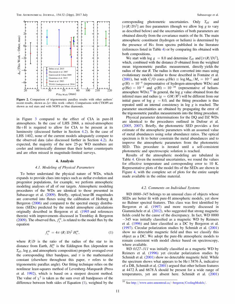
published works for the few overlapping targets. The error barsrepresent both programs’ formal parallax errors added inquadrature for a given target. There are no obvious systematicdifferences with either CTIOPI or NOFS samples.Figure 3 shows an H−R diagram for the astrometric

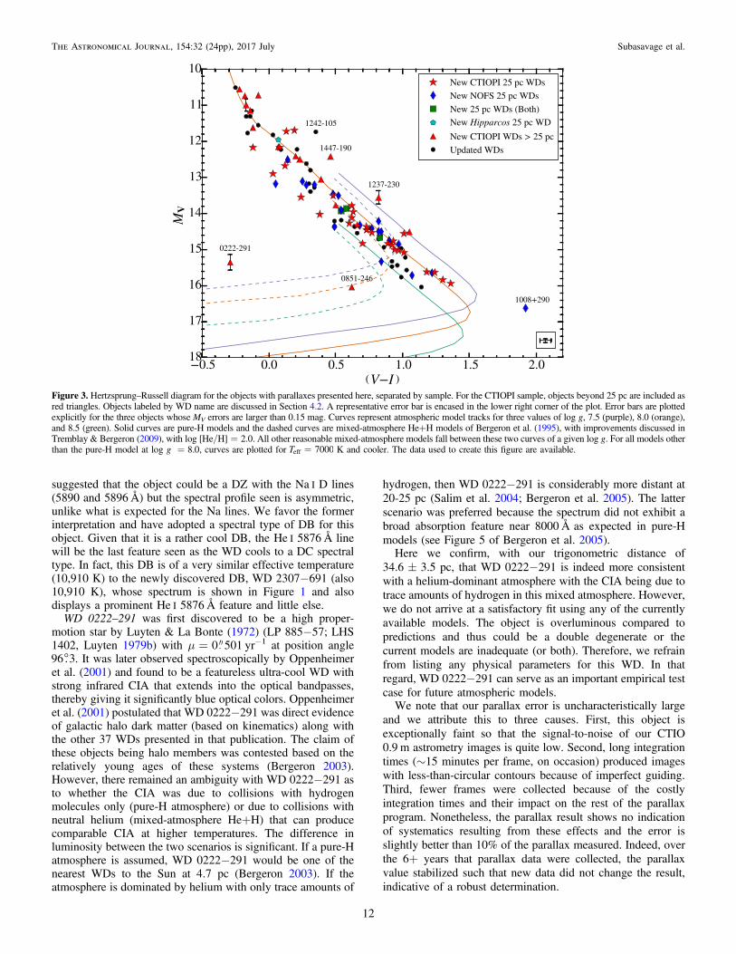
samples presented here. Objects labeled by WD name arediscussed in detail in Section 4.2. Briefly, we find three WDs(WD 1242−105, WD 1447−190, and WD 1237−230) that areoverluminous and aregood candidates for being unresolvedmultiple systems solely based on luminosity. WD 1008+290is a peculiar He-rich DQ WD with exceptional Swan bandabsorption (e.g., Giammichele et al. 2012) such that themeasured V magnitude, whose bandpass encompasses a portionof this absorption, is affected and appears fainter than if theabsorption was not present. Finally, both LHS 2068 (WD 0851−246) and LHS 1402 (WD 0222−291) are very cool WDs thatappear to display collision-induced absorption (CIA) by H2

molecules (Saumon et al. 1994; Hansen 1998; Saumon &Jacobson 1999). CIA opacity is induced by collisionsand thusrequires high atmospheric pressures. High atmospheric pres-sures are reached at much higher effective temperatures in He-rich atmospheres that also contain molecular hydrogenbecauseof the relative transparency of Hecompared topure-H atmo-spheres. Therefore, CIA manifests itself at higher effectivetemperaturesand thus higher luminosities. This effect is shown

7

The Astronomical Journal, 154:32 (24pp), 2017 July Subasavage et al.

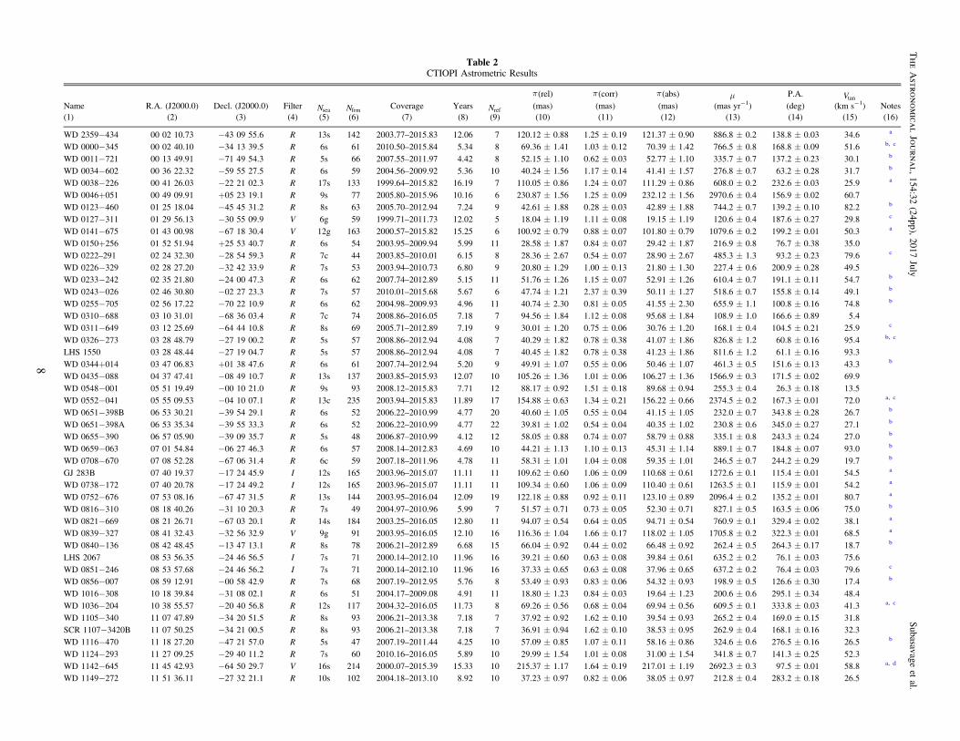
Table 2CTIOPI Astrometric Results

p(rel) p(corr) p(abs) m P.A. Vtan

Name R.A. (J2000.0) Decl. (J2000.0) Filter Nsea Nfrm Coverage Years Nref (mas) (mas) (mas) (mas yr−1) (deg) (km s−1) Notes(1) (2) (3) (4) (5) (6) (7) (8) (9) (10) (11) (12) (13) (14) (15) (16)

WD 2359−434 00 02 10.73 −43 09 55.6 R 13s 142 2003.77–2015.83 12.06 7 120.12±0.88 1.25±0.19 121.37±0.90 886.8±0.2 138.8±0.03 34.6 a

WD 0000−345 00 02 40.10 −34 13 39.5 R 6s 61 2010.50–2015.84 5.34 8 69.36±1.41 1.03±0.12 70.39±1.42 766.5±0.8 168.8±0.09 51.6 b, c

WD 0011−721 00 13 49.91 −71 49 54.3 R 5s 66 2007.55–2011.97 4.42 8 52.15±1.10 0.62±0.03 52.77±1.10 335.7±0.7 137.2±0.23 30.1 b

WD 0034−602 00 36 22.32 −59 55 27.5 R 6s 59 2004.56–2009.92 5.36 10 40.24±1.56 1.17±0.14 41.41±1.57 276.8±0.7 63.2±0.28 31.7 b

WD 0038−226 00 41 26.03 −22 21 02.3 R 17s 133 1999.64–2015.82 16.19 7 110.05±0.86 1.24±0.07 111.29±0.86 608.0±0.2 232.6±0.03 25.9 a

WD 0046+051 00 49 09.91 +05 23 19.1 R 9s 77 2005.80–2015.96 10.16 6 230.87±1.56 1.25±0.09 232.12±1.56 2970.6±0.4 156.9±0.02 60.7WD 0123−460 01 25 18.04 −45 45 31.2 R 8s 63 2005.70–2012.94 7.24 9 42.61±1.88 0.28±0.03 42.89±1.88 744.2±0.7 139.2±0.10 82.2 b

WD 0127−311 01 29 56.13 −30 55 09.9 V 6g 59 1999.71–2011.73 12.02 5 18.04±1.19 1.11±0.08 19.15±1.19 120.6±0.4 187.6±0.27 29.8 c

WD 0141−675 01 43 00.98 −67 18 30.4 V 12g 163 2000.57–2015.82 15.25 6 100.92±0.79 0.88±0.07 101.80±0.79 1079.6±0.2 199.2±0.01 50.3 a

WD 0150+256 01 52 51.94 +25 53 40.7 R 6s 54 2003.95–2009.94 5.99 11 28.58±1.87 0.84±0.07 29.42±1.87 216.9±0.8 76.7±0.38 35.0

WD 0222–291 02 24 32.30 −28 54 59.3 R 7c 44 2003.85–2010.01 6.15 8 28.36±2.67 0.54±0.07 28.90±2.67 485.3±1.3 93.2±0.23 79.6 c

WD 0226−329 02 28 27.20 −32 42 33.9 R 7s 53 2003.94–2010.73 6.80 9 20.80±1.29 1.00±0.13 21.80±1.30 227.4±0.6 200.9±0.28 49.5

WD 0233−242 02 35 21.80 −24 00 47.3 R 6s 62 2007.74–2012.89 5.15 11 51.76±1.26 1.15±0.07 52.91±1.26 610.4±0.7 191.1±0.11 54.7 b

WD 0243−026 02 46 30.80 −02 27 23.3 R 7s 57 2010.01–2015.68 5.67 6 47.74±1.21 2.37±0.39 50.11±1.27 518.6±0.7 155.8±0.14 49.1 b

WD 0255−705 02 56 17.22 −70 22 10.9 R 6s 62 2004.98–2009.93 4.96 11 40.74±2.30 0.81±0.05 41.55±2.30 655.9±1.1 100.8±0.16 74.8 b

WD 0310−688 03 10 31.01 −68 36 03.4 R 7c 74 2008.86–2016.05 7.18 7 94.56±1.84 1.12±0.08 95.68±1.84 108.9±1.0 166.6±0.89 5.4

WD 0311−649 03 12 25.69 −64 44 10.8 R 8s 69 2005.71–2012.89 7.19 9 30.01±1.20 0.75±0.06 30.76±1.20 168.1±0.4 104.5±0.21 25.9 c

WD 0326−273 03 28 48.79 −27 19 00.2 R 5s 57 2008.86–2012.94 4.08 7 40.29±1.82 0.78±0.38 41.07±1.86 826.8±1.2 60.8±0.16 95.4 b, c

LHS 1550 03 28 48.44 −27 19 04.7 R 5s 57 2008.86–2012.94 4.08 7 40.45±1.82 0.78±0.38 41.23±1.86 811.6±1.2 61.1±0.16 93.3

WD 0344+014 03 47 06.83 +01 38 47.6 R 6s 61 2007.74–2012.94 5.20 9 49.91±1.07 0.55±0.06 50.46±1.07 461.3±0.5 151.6±0.13 43.3 b

WD 0435−088 04 37 47.41 −08 49 10.7 R 13s 137 2003.85–2015.93 12.07 10 105.26±1.36 1.01±0.06 106.27±1.36 1566.9±0.3 171.5±0.02 69.9

WD 0548−001 05 51 19.49 −00 10 21.0 R 9s 93 2008.12–2015.83 7.71 12 88.17±0.92 1.51±0.18 89.68±0.94 255.3±0.4 26.3±0.18 13.5WD 0552−041 05 55 09.53 −04 10 07.1 R 13c 235 2003.94–2015.83 11.89 17 154.88±0.63 1.34±0.21 156.22±0.66 2374.5±0.2 167.3±0.01 72.0 a, c

WD 0651−398B 06 53 30.21 −39 54 29.1 R 6s 52 2006.22–2010.99 4.77 20 40.60±1.05 0.55±0.04 41.15±1.05 232.0±0.7 343.8±0.28 26.7 b

WD 0651−398A 06 53 35.34 −39 55 33.3 R 6s 52 2006.22–2010.99 4.77 22 39.81±1.02 0.54±0.04 40.35±1.02 230.8±0.6 345.0±0.27 27.1 b

WD 0655−390 06 57 05.90 −39 09 35.7 R 5s 48 2006.87–2010.99 4.12 12 58.05±0.88 0.74±0.07 58.79±0.88 335.1±0.8 243.3±0.24 27.0 b

WD 0659−063 07 01 54.84 −06 27 46.3 R 6s 57 2008.14–2012.83 4.69 10 44.21±1.13 1.10±0.13 45.31±1.14 889.1±0.7 184.8±0.07 93.0 b

WD 0708−670 07 08 52.28 −67 06 31.4 R 6c 59 2007.18–2011.96 4.78 11 58.31±1.01 1.04±0.08 59.35±1.01 246.5±0.7 244.2±0.29 19.7 b

GJ 283B 07 40 19.37 −17 24 45.9 I 12s 165 2003.96–2015.07 11.11 11 109.62±0.60 1.06±0.09 110.68±0.61 1272.6±0.1 115.4±0.01 54.5 a

WD 0738−172 07 40 20.78 −17 24 49.2 I 12s 165 2003.96–2015.07 11.11 11 109.34±0.60 1.06±0.09 110.40±0.61 1263.5±0.1 115.9±0.01 54.2 a

WD 0752−676 07 53 08.16 −67 47 31.5 R 13s 144 2003.95–2016.04 12.09 19 122.18±0.88 0.92±0.11 123.10±0.89 2096.4±0.2 135.2±0.01 80.7 a

WD 0816−310 08 18 40.26 −31 10 20.3 R 7s 49 2004.97–2010.96 5.99 7 51.57±0.71 0.73±0.05 52.30±0.71 827.1±0.5 163.5±0.06 75.0 b

WD 0821−669 08 21 26.71 −67 03 20.1 R 14s 184 2003.25–2016.05 12.80 11 94.07±0.54 0.64±0.05 94.71±0.54 760.9±0.1 329.4±0.02 38.1 a

WD 0839−327 08 41 32.43 −32 56 32.9 V 9g 91 2003.95–2016.05 12.10 16 116.36±1.04 1.66±0.17 118.02±1.05 1705.8±0.2 322.3±0.01 68.5 a

WD 0840−136 08 42 48.45 −13 47 13.1 R 8s 78 2006.21–2012.89 6.68 15 66.04±0.92 0.44±0.02 66.48±0.92 262.4±0.5 264.3±0.17 18.7 b

LHS 2067 08 53 56.35 −24 46 56.5 I 7s 71 2000.14–2012.10 11.96 16 39.21±0.60 0.63±0.08 39.84±0.61 635.2±0.2 76.1±0.03 75.6

WD 0851−246 08 53 57.68 −24 46 56.2 I 7s 71 2000.14–2012.10 11.96 16 37.33±0.65 0.63±0.08 37.96±0.65 637.2±0.2 76.4±0.03 79.6 c

WD 0856−007 08 59 12.91 −00 58 42.9 R 7s 68 2007.19–2012.95 5.76 8 53.49±0.93 0.83±0.06 54.32±0.93 198.9±0.5 126.6±0.30 17.4 b

WD 1016−308 10 18 39.84 −31 08 02.1 R 6s 51 2004.17–2009.08 4.91 11 18.80±1.23 0.84±0.03 19.64±1.23 200.6±0.6 295.1±0.34 48.4

WD 1036−204 10 38 55.57 −20 40 56.8 R 12s 117 2004.32–2016.05 11.73 8 69.26±0.56 0.68±0.04 69.94±0.56 609.5±0.1 333.8±0.03 41.3 a, c

WD 1105−340 11 07 47.89 −34 20 51.5 R 8s 93 2006.21–2013.38 7.18 7 37.92±0.92 1.62±0.10 39.54±0.93 265.2±0.4 169.0±0.15 31.8SCR 1107−3420B 11 07 50.25 −34 21 00.5 R 8s 93 2006.21–2013.38 7.18 7 36.91±0.94 1.62±0.10 38.53±0.95 262.9±0.4 168.1±0.16 32.3

WD 1116−470 11 18 27.20 −47 21 57.0 R 5s 47 2007.19–2011.44 4.25 10 57.09±0.85 1.07±0.11 58.16±0.86 324.6±0.6 276.5±0.16 26.5 b

WD 1124−293 11 27 09.25 −29 40 11.2 R 7s 60 2010.16–2016.05 5.89 10 29.99±1.54 1.01±0.08 31.00±1.54 341.8±0.7 141.3±0.25 52.3

WD 1142−645 11 45 42.93 −64 50 29.7 V 16s 214 2000.07–2015.39 15.33 10 215.37±1.17 1.64±0.19 217.01±1.19 2692.3±0.3 97.5±0.01 58.8 a, d

WD 1149−272 11 51 36.11 −27 32 21.1 R 10s 102 2004.18–2013.10 8.92 10 37.23±0.97 0.82±0.06 38.05±0.97 212.8±0.4 283.2±0.18 26.5

8

TheAstro

nomica

lJourn

al,

154:32(24pp),

2017July

Subasavage

etal.

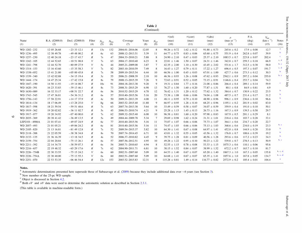
Table 2(Continued)

p(rel) p(corr) p(abs) m P.A. Vtan

Name R.A. (J2000.0) Decl. (J2000.0) Filter Nsea NfrmCoverage Years Nref (mas) (mas) (mas) (mas yr−1) (deg) (km s−1) Notes

(1) (2) (3) (4) (5) (6) (7) (8) (9) (10) (11) (12) (13) (14) (15) (16)

WD 1202−232 12 05 26.68 −23 33 12.1 R 13s 132 2004.01–2016.06 12.05 8 90.26±0.72 1.62±0.12 91.88±0.73 245.6±0.2 17.9±0.08 12.7 a

WD 1236−495 12 38 49.78 −49 48 00.2 R 6c 63 2008.12–2013.51 5.39 11 64.77±0.75 0.83±0.06 65.60±0.75 551.9±0.4 262.8±0.07 39.9 b

WD 1237−230 12 40 24.18 −23 17 43.7 R 7s 47 2004.33–2010.21 5.88 8 24.90±2.10 0.47±0.03 25.37±2.10 1083.5±0.7 223.8±0.07 202.4 c

WD 1242−105 12 44 52.65 −10 51 08.8 V 7s 63 2004.17–2010.40 6.23 8 22.81±1.46 1.50±0.07 24.31±1.46 342.8±0.7 259.3±0.18 66.9 c, d

WD 1241−798 12 44 52.70 −80 09 27.9 V 5s 44 2005.21–2009.08 3.87 7 42.35±2.00 1.10±0.30 43.45±2.02 531.6±1.7 312.5±0.38 58.0 b, c

WD 1314−153 13 16 43.60 −15 35 58.3 V 7s 82 2003.10–2010.59 7.49 8 16.43±1.27 0.79±0.11 17.22±1.27 696.4±0.5 197.3±0.07 191.7 c, d

WD 1338+052 13 41 21.80 +05 00 45.8 R 7s 58 2009.10–2015.54 6.44 10 66.56±1.00 0.45±0.03 67.01±1.00 427.7±0.6 273.3±0.12 30.3 b

WD 1339−340 13 42 02.88 −34 15 19.4 R 3c 55 2006.21–2008.39 2.18 10 46.36±0.93 1.26±0.08 47.62±0.93 2562.1±0.9 297.2±0.04 255.0 b, c

WD 1444−174 14 47 25.34 −17 42 15.8 R 8s 79 2008.13–2015.39 7.26 9 72.63±0.91 0.52±0.05 73.15±0.91 1146.6±0.4 253.7±0.04 74.3

WD 1447−190 14 50 11.93 −19 14 08.7 R 10s 91 2004.18–2013.38 9.20 9 19.31±0.84 1.77±0.16 21.08±0.86 266.4±0.4 289.1±0.14 59.9 c

WD 1620−391 16 23 33.83 −39 13 46.1 R 8s 73 2008.31–2015.29 6.98 13 76.27±1.50 1.60±0.20 77.87±1.51 80.1±0.8 84.9±0.81 4.9

WD 1630+089 16 32 33.17 +08 51 22.7 R 6s 56 2010.52–2015.29 4.78 12 76.42±1.31 1.20±0.12 77.62±1.32 384.4±0.7 130.9±0.22 23.5 b

WD 1743−545 17 47 36.81 −54 36 31.2 R 6s 57 2010.40–2015.56 5.16 20 73.38±1.08 0.66±0.06 74.04±1.08 487.5±0.7 231.4±0.17 31.2 b

WD 1756+143 17 58 22.91 +14 17 37.9 R 4c 50 2009.31–2013.39 4.08 11 48.11±0.95 0.79±0.10 48.90±0.96 996.1±0.9 236.6±0.10 96.6 b

WD 1814+134 18 17 06.49 +13 28 25.0 V 8g 66 2003.52–2015.40 11.88 9 66.97±0.95 1.28±0.10 68.25±0.96 1195.1±0.2 201.9±0.02 83.0 c

WD 1817−598 18 21 59.54 −59 51 48.6 R 7s 63 2007.74–2013.38 5.64 10 33.49±0.59 0.58±0.07 34.07±0.59 359.9±0.4 191.0±0.10 50.1

WD 1919−362 19 20 02.82 −36 11 02.7 R 5s 45 2006.53–2010.74 4.21 9 25.28±1.15 1.45±0.13 26.73±1.16 167.3±0.9 139.5±0.58 29.7

WD 1917−077 19 20 34.92 −07 40 00.0 R 7s 62 2009.32–2015.40 6.08 10 96.38±0.81 1.60±0.20 97.98±0.83 167.9±0.5 201.1±0.29 8.1WD 2035−369 20 38 41.42 −36 49 13.5 R 5s 49 2004.44–2009.78 5.34 7 29.69±0.98 1.62±0.24 31.31±1.01 218.4±0.6 103.7±0.28 33.1

LEP2101−4906A 21 01 07.41 −49 07 24.9 R 6c 77 2010.40–2015.56 5.16 11 75.07±1.07 0.66±0.06 75.73±1.07 364.1±0.6 234.7±0.20 22.7

WD 2057−493 21 01 05.21 −49 06 24.2 R 6c 81 2010.40–2015.56 5.16 11 74.47±1.03 0.66±0.06 75.13±1.03 368.6±0.6 234.0±0.19 23.3 b, c

WD 2105−820 21 13 16.81 −81 49 12.8 R 7s 52 2009.54–2015.37 5.82 10 64.30±1.41 0.67±0.08 64.97±1.41 452.0±0.8 144.9±0.20 33.0 b

WD 2118−388 21 22 05.59 −38 38 34.8 R 8s 70 2007.74–2014.45 6.71 10 43.01±1.32 0.55±0.05 43.56±1.32 176.8±0.7 108.6±0.39 19.2 b

WD 2133−135 21 36 16.39 −13 18 34.5 R 4s 52 2006.37–2010.82 4.45 9 39.75±1.28 0.81±0.09 40.56±1.28 293.6±0.6 117.2±0.23 34.3 b

WD 2159−754 22 04 20.84 −75 13 26.1 R 6s 57 2007.56–2012.51 4.95 10 49.28±1.22 0.95±0.10 50.23±1.22 539.8±0.7 278.5±0.13 50.9 b, c

WD 2211−392 22 14 34.75 −38 59 07.3 R 6s 54 2005.71–2010.65 4.94 8 52.55±1.15 0.78±0.08 53.33±1.15 1075.3±0.6 110.1±0.06 95.6

WD 2216−657 22 19 48.32 −65 29 17.6 R 7s 62 2004.90–2011.71 6.81 10 38.15±1.52 0.84±0.07 38.99±1.52 672.2±0.7 163.7±0.10 81.7

WD 2226−754B 22 30 33.55 −75 15 24.2 V 6s 60 2002.51–2007.60 5.09 10 64.53±1.40 0.67±0.07 65.20±1.40 1867.3±1.0 167.3±0.05 135.8 b, c, d

WD 2226−754A 22 30 40.00 −75 13 55.3 V 6s 60 2002.51–2007.60 5.09 10 64.68±1.41 0.67±0.07 65.35±1.41 1857.6±1.0 167.8±0.05 134.7 b, c, d

WD 2251−070 22 53 53.35 −06 46 54.4 R 12s 153 2003.52–2015.83 12.31 8 115.28±0.81 1.49±0.14 116.77±0.82 2572.9±0.2 105.4±0.01 104.4 a

Notes.a Astrometric determinations presented here supersede those of Subasavage et al. (2009) because they include additional data over ∼6 years (see Section 3).b New member of the 25-pc WD sample.c Object is discussed in Section 4.2.d Both oV nVand data were used to determine the astrometric solution as described in Section 2.3.1.

(This table is available in machine-readable form.)

9

TheAstro

nomica

lJourn

al,

154:32(24pp),

2017July

Subasavage

etal.

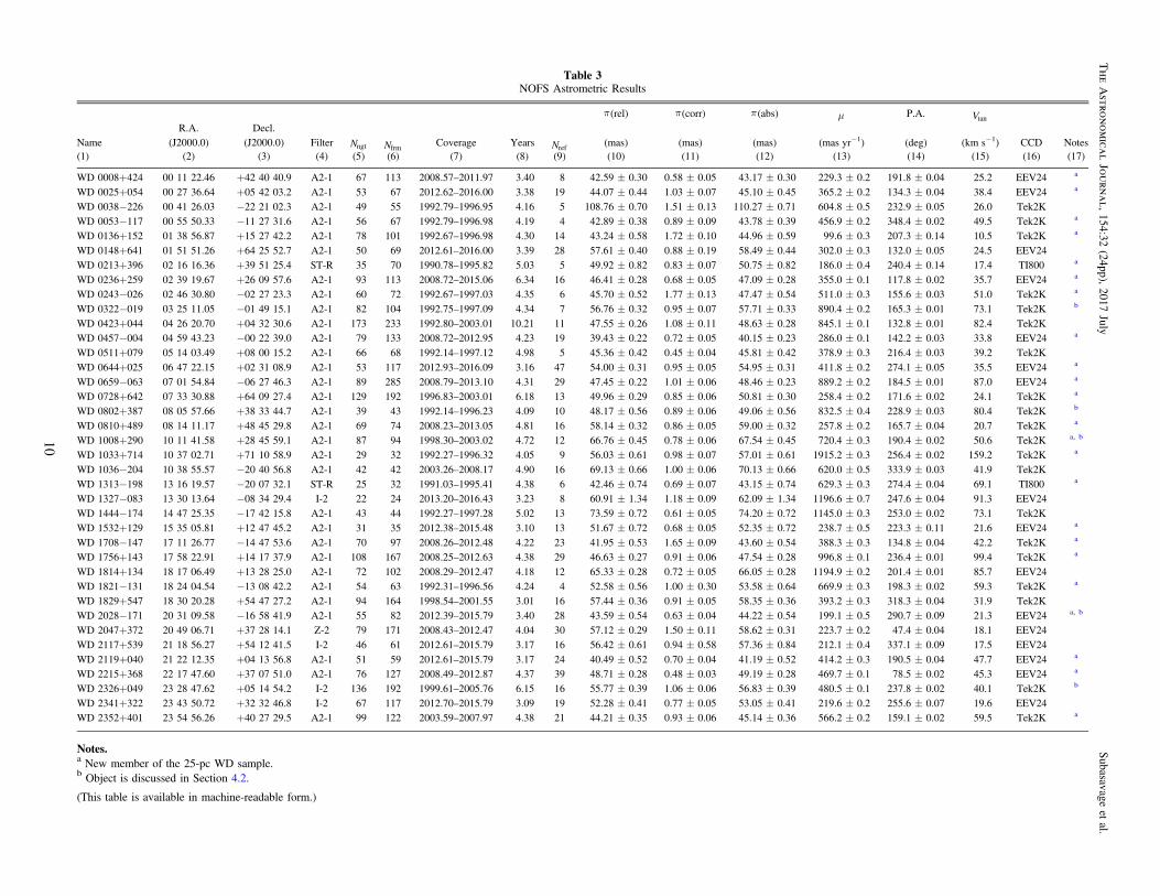
Table 3NOFS Astrometric Results

p(rel) p(corr) p(abs) m P.A. Vtan

NameR.A.

(J2000.0)Decl.

(J2000.0) Filter Nngt NfrmCoverage Years Nref (mas) (mas) (mas) (mas yr−1) (deg) (km s−1) CCD Notes

(1) (2) (3) (4) (5) (6) (7) (8) (9) (10) (11) (12) (13) (14) (15) (16) (17)

WD 0008+424 00 11 22.46 +42 40 40.9 A2-1 67 113 2008.57–2011.97 3.40 8 42.59±0.30 0.58±0.05 43.17±0.30 229.3±0.2 191.8±0.04 25.2 EEV24 a

WD 0025+054 00 27 36.64 +05 42 03.2 A2-1 53 67 2012.62–2016.00 3.38 19 44.07±0.44 1.03±0.07 45.10±0.45 365.2±0.2 134.3±0.04 38.4 EEV24 a

WD 0038−226 00 41 26.03 −22 21 02.3 A2-1 49 55 1992.79–1996.95 4.16 5 108.76±0.70 1.51±0.13 110.27±0.71 604.8±0.5 232.9±0.05 26.0 Tek2K

WD 0053−117 00 55 50.33 −11 27 31.6 A2-1 56 67 1992.79–1996.98 4.19 4 42.89±0.38 0.89±0.09 43.78±0.39 456.9±0.2 348.4±0.02 49.5 Tek2K a

WD 0136+152 01 38 56.87 +15 27 42.2 A2-1 78 101 1992.67–1996.98 4.30 14 43.24±0.58 1.72±0.10 44.96±0.59 99.6±0.3 207.3±0.14 10.5 Tek2K a

WD 0148+641 01 51 51.26 +64 25 52.7 A2-1 50 69 2012.61–2016.00 3.39 28 57.61±0.40 0.88±0.19 58.49±0.44 302.0±0.3 132.0±0.05 24.5 EEV24

WD 0213+396 02 16 16.36 +39 51 25.4 ST-R 35 70 1990.78–1995.82 5.03 5 49.92±0.82 0.83±0.07 50.75±0.82 186.0±0.4 240.4±0.14 17.4 TI800 a

WD 0236+259 02 39 19.67 +26 09 57.6 A2-1 93 113 2008.72–2015.06 6.34 16 46.41±0.28 0.68±0.05 47.09±0.28 355.0±0.1 117.8±0.02 35.7 EEV24 a

WD 0243−026 02 46 30.80 −02 27 23.3 A2-1 60 72 1992.67–1997.03 4.35 6 45.70±0.52 1.77±0.13 47.47±0.54 511.0±0.3 155.6±0.03 51.0 Tek2K a

WD 0322−019 03 25 11.05 −01 49 15.1 A2-1 82 104 1992.75–1997.09 4.34 7 56.76±0.32 0.95±0.07 57.71±0.33 890.4±0.2 165.3±0.01 73.1 Tek2K b

WD 0423+044 04 26 20.70 +04 32 30.6 A2-1 173 233 1992.80–2003.01 10.21 11 47.55±0.26 1.08±0.11 48.63±0.28 845.1±0.1 132.8±0.01 82.4 Tek2KWD 0457−004 04 59 43.23 −00 22 39.0 A2-1 79 133 2008.72–2012.95 4.23 19 39.43±0.22 0.72±0.05 40.15±0.23 286.0±0.1 142.2±0.03 33.8 EEV24 a

WD 0511+079 05 14 03.49 +08 00 15.2 A2-1 66 68 1992.14–1997.12 4.98 5 45.36±0.42 0.45±0.04 45.81±0.42 378.9±0.3 216.4±0.03 39.2 Tek2K

WD 0644+025 06 47 22.15 +02 31 08.9 A2-1 53 117 2012.93–2016.09 3.16 47 54.00±0.31 0.95±0.05 54.95±0.31 411.8±0.2 274.1±0.05 35.5 EEV24 a

WD 0659−063 07 01 54.84 −06 27 46.3 A2-1 89 285 2008.79–2013.10 4.31 29 47.45±0.22 1.01±0.06 48.46±0.23 889.2±0.2 184.5±0.01 87.0 EEV24 a

WD 0728+642 07 33 30.88 +64 09 27.4 A2-1 129 192 1996.83–2003.01 6.18 13 49.96±0.29 0.85±0.06 50.81±0.30 258.4±0.2 171.6±0.02 24.1 Tek2K a

WD 0802+387 08 05 57.66 +38 33 44.7 A2-1 39 43 1992.14–1996.23 4.09 10 48.17±0.56 0.89±0.06 49.06±0.56 832.5±0.4 228.9±0.03 80.4 Tek2K b

WD 0810+489 08 14 11.17 +48 45 29.8 A2-1 69 74 2008.23–2013.05 4.81 16 58.14±0.32 0.86±0.05 59.00±0.32 257.8±0.2 165.7±0.04 20.7 Tek2K a

WD 1008+290 10 11 41.58 +28 45 59.1 A2-1 87 94 1998.30–2003.02 4.72 12 66.76±0.45 0.78±0.06 67.54±0.45 720.4±0.3 190.4±0.02 50.6 Tek2K a, b

WD 1033+714 10 37 02.71 +71 10 58.9 A2-1 29 32 1992.27–1996.32 4.05 9 56.03±0.61 0.98±0.07 57.01±0.61 1915.2±0.3 256.4±0.02 159.2 Tek2K a

WD 1036−204 10 38 55.57 −20 40 56.8 A2-1 42 42 2003.26–2008.17 4.90 16 69.13±0.66 1.00±0.06 70.13±0.66 620.0±0.5 333.9±0.03 41.9 Tek2K

WD 1313−198 13 16 19.57 −20 07 32.1 ST-R 25 32 1991.03–1995.41 4.38 6 42.46±0.74 0.69±0.07 43.15±0.74 629.3±0.3 274.4±0.04 69.1 TI800 a

WD 1327−083 13 30 13.64 −08 34 29.4 I-2 22 24 2013.20–2016.43 3.23 8 60.91±1.34 1.18±0.09 62.09±1.34 1196.6±0.7 247.6±0.04 91.3 EEV24

WD 1444−174 14 47 25.35 −17 42 15.8 A2-1 43 44 1992.27–1997.28 5.02 13 73.59±0.72 0.61±0.05 74.20±0.72 1145.0±0.3 253.0±0.02 73.1 Tek2K

WD 1532+129 15 35 05.81 +12 47 45.2 A2-1 31 35 2012.38–2015.48 3.10 13 51.67±0.72 0.68±0.05 52.35±0.72 238.7±0.5 223.3±0.11 21.6 EEV24 a

WD 1708−147 17 11 26.77 −14 47 53.6 A2-1 70 97 2008.26–2012.48 4.22 23 41.95±0.53 1.65±0.09 43.60±0.54 388.3±0.3 134.8±0.04 42.2 Tek2K a

WD 1756+143 17 58 22.91 +14 17 37.9 A2-1 108 167 2008.25–2012.63 4.38 29 46.63±0.27 0.91±0.06 47.54±0.28 996.8±0.1 236.4±0.01 99.4 Tek2K a

WD 1814+134 18 17 06.49 +13 28 25.0 A2-1 72 102 2008.29–2012.47 4.18 12 65.33±0.28 0.72±0.05 66.05±0.28 1194.9±0.2 201.4±0.01 85.7 EEV24

WD 1821−131 18 24 04.54 −13 08 42.2 A2-1 54 63 1992.31–1996.56 4.24 4 52.58±0.56 1.00±0.30 53.58±0.64 669.9±0.3 198.3±0.02 59.3 Tek2K a

WD 1829+547 18 30 20.28 +54 47 27.2 A2-1 94 164 1998.54–2001.55 3.01 16 57.44±0.36 0.91±0.05 58.35±0.36 393.2±0.3 318.3±0.04 31.9 Tek2KWD 2028−171 20 31 09.58 −16 58 41.9 A2-1 55 82 2012.39–2015.79 3.40 28 43.59±0.54 0.63±0.04 44.22±0.54 199.1±0.5 290.7±0.09 21.3 EEV24 a, b

WD 2047+372 20 49 06.71 +37 28 14.1 Z-2 79 171 2008.43–2012.47 4.04 30 57.12±0.29 1.50±0.11 58.62±0.31 223.7±0.2 47.4±0.04 18.1 EEV24

WD 2117+539 21 18 56.27 +54 12 41.5 I-2 46 61 2012.61–2015.79 3.17 16 56.42±0.61 0.94±0.58 57.36±0.84 212.1±0.4 337.1±0.09 17.5 EEV24

WD 2119+040 21 22 12.35 +04 13 56.8 A2-1 51 59 2012.61–2015.79 3.17 24 40.49±0.52 0.70±0.04 41.19±0.52 414.2±0.3 190.5±0.04 47.7 EEV24 a

WD 2215+368 22 17 47.60 +37 07 51.0 A2-1 76 127 2008.49–2012.87 4.37 39 48.71±0.28 0.48±0.03 49.19±0.28 469.7±0.1 78.5±0.02 45.3 EEV24 a

WD 2326+049 23 28 47.62 +05 14 54.2 I-2 136 192 1999.61–2005.76 6.15 16 55.77±0.39 1.06±0.06 56.83±0.39 480.5±0.1 237.8±0.02 40.1 Tek2K b

WD 2341+322 23 43 50.72 +32 32 46.8 I-2 67 117 2012.70–2015.79 3.09 19 52.28±0.41 0.77±0.05 53.05±0.41 219.6±0.2 255.6±0.07 19.6 EEV24WD 2352+401 23 54 56.26 +40 27 29.5 A2-1 99 122 2003.59–2007.97 4.38 21 44.21±0.35 0.93±0.06 45.14±0.36 566.2±0.2 159.1±0.02 59.5 Tek2K a

Notes.a New member of the 25-pc WD sample.b Object is discussed in Section 4.2.

(This table is available in machine-readable form.)

10

TheAstro

nomica

lJourn

al,

154:32(24pp),

2017July

Subasavage

etal.

in Figure 3 compared to the effect of CIA in pure-Hatmospheres. In the case of LHS 2068, a mixed-atmosphereHe+H is required to allow for CIA to be present at itsluminosity (discussed further in Section 4.2). In the case ofLHS 1402, none of the current modelsadequately comparetothe observed data (also discussed further in Section 4.2). Asexpected, the majority of the new 25-pc WD members arecooler and intrinsically dimmer than their hotter counterpartsand are often missed in magnitude-limited surveys.

4. Analysis

4.1. Modeling of Physical Parameters

To better understand the physical nature of WDs, whichexpandsto provide clues into topics such as stellar evolution andprogenitor populations, for example, we perform atmosphericmodeling analyses of all of our targets. Atmospheric modelingprocedures of the WDs are identical to those presented inSubasavage et al. (2009). Briefly, optical/near-IR magnitudesare converted into fluxes using the calibration of Holberg &Bergeron (2006) and compared to the spectral energy distribu-tions (SEDs) predicted by the model atmosphere calculationsoriginally described in Bergeron et al. (1995and referencestherein) with improvements discussed in Tremblay & Bergeron(2009). The observed flux, lf

m, is related to the model flux by theequation

p=l l( ) ( )f R D H4 , 1m m2

where R/D is the ratio of the radius of the star to itsdistance from Earth, lHm is the Eddington flux (dependent onTeff , log g, and atmospheric composition) properly averaged overthe corresponding filter bandpass, and π is the mathematicalconstant (elsewhere throughout this paper, π refers to thetrigonometric parallax angle). Our fitting technique relies on thenonlinear least-squares method of Levenberg–Marquardt (Presset al. 1992), which is based on a steepest descent method.The value of c2 is taken as the sum over all bandpasses of thedifference between both sides of Equation (1), weighted by the

corresponding photometric uncertainties. Only Teff andp[ ( ) ]R D 2 are free parameters (though we allow log g to varyas described below) and the uncertainties of both parameters areobtained directly from the covariance matrix of the fit. The mainatmospheric constituent (hydrogen or helium) is determined bythe presence of Hα from spectra published in the literature(references listed in Table 4) or by comparing fits obtained withboth compositions.We start with log g =8.0 and determine Teff and p[ ( )R D 2],

which, combined with the distance D obtained from the weightedmean trigonometric parallax measurement, directlyyieldstheradius of the star R. The radius is then converted into mass usingevolutionary models similar to those described in Fontaine et al.(2001), but with C/O cores º = -( )q M MHe log 10He

2 and= -( )q H 10 4 (representative of hydrogen-atmosphere WDs)and= -( )q He 10 2 and = -( )q H 10 10 (representative of helium-

atmosphere WDs).10 In general, the log g value obtained from theinferred mass and radius ( =g GM R2) will be different from ourinitial guess of log g =8.0, and the fitting procedure is thusrepeated until an internal consistency in log g is reached. Theparameter uncertainties are obtained by propagating the error ofthe trigonometric parallax measurements into the fitting procedure.Physical parameter determinations for the DQ and DZ WDs

are identical to the procedures outlined in Dufour et al.(2005, 2007). Briefly, the photometric SED provides a firstestimate of the atmospheric parameters with an assumed valueof metal abundances using solar abundance ratios. The opticalspectrum is fit to better constrain the metal abundances and toimprove the atmospheric parameters from the photometricSED. This procedure is iterated until a self-consistentphotometric and spectroscopic solution is reached.Results of the atmospheric modeling are tabulated in

Table 4. Given the nominal uncertainties, we round the valuesfor effective temperature and corresponding error to 10 K.Representative plots of the model fits of the SEDs are shown inFigure 4, with the complete set of plots for the entire samplemade available in the online material.

4.2. Comments on Individual Systems

WD 0000–345 belongs to an unusual class of objects whoseSEDs are better fit with pure-H atmospheric models, yet showno Balmer spectral features. This class was first identified byBergeron et al. (1997) and more recently discussed inGiammichele et al. (2012), who suggested that strong magneticfields could be the cause of the discrepancy. In fact, WD 0000−345 was initially classified as a magnetic WD by Reimerset al. (1996) and later classified as a DC by Bergeron et al.(1997). Circular polarization studies by Schmidt et al. (2001)show no detectable magnetic fieldand thus we classify thisobject as a DC. We adopt the pure-He atmospheric models toremain consistent with model choice based on spectroscopy,where available.WD 0127–311 was initially classified as a magnetic WD by

Reimers et al. (1996) yet circular polarization studies bySchmidt et al. (2001) show no detectable magnetic field. Whilethe spectrum shows what appears to be He I 5876 Å, indicativeof a DB, Schmidt et al. (2001) argued that other helium featuresat 4472 Åand 6678 Åshould be present for a wide range oftemperatures, yet are absent here. Schmidt et al. (2001)

Figure 2. Comparison of trigonometric parallax results with other authors’recent results, shown as pD (this work−other). Comparisons with CTIOPI areshown as red stars and with NOFS as blue diamonds.

10 See http://www.astro.umontreal.ca/~bergeron/CoolingModels/.

11

The Astronomical Journal, 154:32 (24pp), 2017 July Subasavage et al.

suggested that the object could be a DZ with the Na I D lines(5890 and 5896 Å) but the spectral profile seen is asymmetric,unlike what is expected for the Na lines. We favor the formerinterpretation and have adopted a spectral type of DB for thisobject. Given that it is a rather cool DB, the He I 5876 Ålinewill be the last feature seen as the WD cools to a DC spectraltype. In fact, this DB is of a very similar effective temperature(10,910 K) to the newly discovered DB, WD 2307−691 (also10,910 K), whose spectrum is shown in Figure 1 and alsodisplays a prominent He I 5876 Åfeature and little else.

WD 0222–291 was first discovered to be a high proper-motion star by Luyten & La Bonte (1972) (LP 885−57; LHS1402, Luyten 1979b) with μ=0 501 yr−1 at position angle

96 .3. It was later observed spectroscopically by Oppenheimeret al. (2001) and found to be a featureless ultra-cool WD withstrong infrared CIA that extends into the optical bandpasses,thereby giving it significantly blue optical colors. Oppenheimeret al. (2001) postulated that WD 0222−291 was direct evidenceof galactic halo dark matter (based on kinematics) along withthe other 37 WDs presented in that publication. The claim ofthese objects being halo members was contested based on therelatively young ages of these systems (Bergeron 2003).However, there remained an ambiguity with WD 0222−291 asto whether the CIA was due to collisions with hydrogenmolecules only (pure-H atmosphere) or due to collisions withneutral helium (mixed-atmosphere He+H) that can producecomparable CIA at higher temperatures. The difference inluminosity between the two scenarios is significant. If a pure-Hatmosphere is assumed, WD 0222−291 would be one of thenearest WDs to the Sun at 4.7 pc (Bergeron 2003). If theatmosphere is dominated by helium with only trace amounts of

hydrogen, then WD 0222−291 is considerably more distant at20-25 pc (Salim et al. 2004; Bergeron et al. 2005). The latterscenario was preferred because the spectrum did not exhibit abroad absorption feature near 8000 Åas expected in pure-Hmodels (see Figure 5 of Bergeron et al. 2005).Here we confirm, with our trigonometric distance of

34.6±3.5 pc, that WD 0222−291 is indeed more consistentwith a helium-dominant atmosphere with the CIA being due totrace amounts of hydrogen in this mixed atmosphere. However,we do not arrive at a satisfactory fit using any of the currentlyavailable models. The object is overluminous compared topredictions and thus could be a double degenerate or thecurrent models are inadequate (or both). Therefore, we refrainfrom listing any physical parameters for this WD. In thatregard, WD 0222−291 can serve as an important empirical testcase for future atmospheric models.We note that our parallax error is uncharacteristically large

and we attribute this to three causes. First, this object isexceptionally faint so that the signal-to-noise of our CTIO0.9 m astrometry images is quite low. Second, long integrationtimes (∼15 minutes per frame, on occasion)produced imageswith less-than-circular contours because of imperfect guiding.Third, fewer frames were collected because of the costlyintegration times and their impact on the rest of the parallaxprogram. Nonetheless, the parallax result shows no indicationof systematics resulting from these effects and the error isslightly better than 10% of the parallax measured. Indeed, overthe 6+ years that parallax data were collected, the parallaxvalue stabilized such that new data did not change the result,indicative of a robust determination.

Figure 3. Hertzsprung–Russell diagram for the objects with parallaxes presented here, separated by sample. For the CTIOPI sample, objects beyond 25 pc are included asred triangles. Objects labeled by WD name are discussed in Section 4.2. A representative error bar is encased in the lower right corner of the plot. Error bars are plottedexplicitly for the three objects whose MV errors are larger than 0.15 mag. Curves represent atmospheric model tracks for three values of log g, 7.5 (purple), 8.0 (orange),and 8.5 (green). Solid curves are pure-H models and the dashed curves are mixed-atmosphere He+H models of Bergeron et al. (1995), with improvements discussed inTremblay & Bergeron (2009), with log [He/H]=2.0. All other reasonable mixed-atmosphere models fall between these two curves of a given log g. For all models otherthan the pure-H model at log g =8.0, curves are plotted for =T 7000eff K and cooler. The data used to create this figure are available.

12

The Astronomical Journal, 154:32 (24pp), 2017 July Subasavage et al.

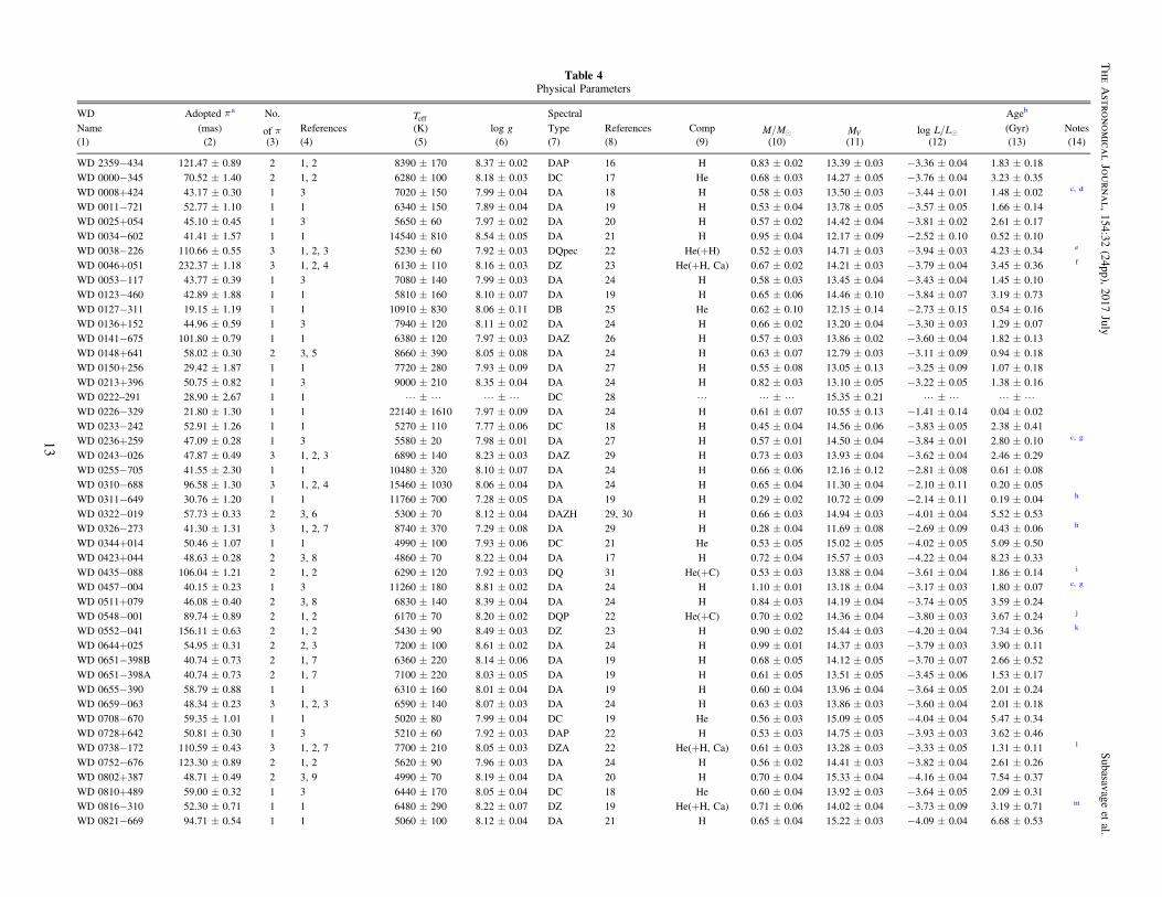
Table 4Physical Parameters

WD Adopted pa No. Teff Spectral Ageb

Name (mas) of p References (K) log g Type References Comp M/ M MV log L/ L (Gyr) Notes(1) (2) (3) (4) (5) (6) (7) (8) (9) (10) (11) (12) (13) (14)

WD 2359−434 121.47±0.89 2 1, 2 8390±170 8.37±0.02 DAP 16 H 0.83±0.02 13.39±0.03 −3.36±0.04 1.83±0.18

WD 0000−345 70.52±1.40 2 1, 2 6280±100 8.18±0.03 DC 17 He 0.68±0.03 14.27±0.05 −3.76±0.04 3.23±0.35

WD 0008+424 43.17±0.30 1 3 7020±150 7.99±0.04 DA 18 H 0.58±0.03 13.50±0.03 −3.44±0.01 1.48±0.02 c, d

WD 0011−721 52.77±1.10 1 1 6340±150 7.89±0.04 DA 19 H 0.53±0.04 13.78±0.05 −3.57±0.05 1.66±0.14

WD 0025+054 45.10±0.45 1 3 5650±60 7.97±0.02 DA 20 H 0.57±0.02 14.42±0.04 −3.81±0.02 2.61±0.17

WD 0034−602 41.41±1.57 1 1 14540±810 8.54±0.05 DA 21 H 0.95±0.04 12.17±0.09 −2.52±0.10 0.52±0.10WD 0038−226 110.66±0.55 3 1, 2, 3 5230±60 7.92±0.03 DQpec 22 He(+H) 0.52±0.03 14.71±0.03 −3.94±0.03 4.23±0.34 e

WD 0046+051 232.37±1.18 3 1, 2, 4 6130±110 8.16±0.03 DZ 23 He(+H, Ca) 0.67±0.02 14.21±0.03 −3.79±0.04 3.45±0.36 f

WD 0053−117 43.77±0.39 1 3 7080±140 7.99±0.03 DA 24 H 0.58±0.03 13.45±0.04 −3.43±0.04 1.45±0.10

WD 0123−460 42.89±1.88 1 1 5810±160 8.10±0.07 DA 19 H 0.65±0.06 14.46±0.10 −3.84±0.07 3.19±0.73

WD 0127−311 19.15±1.19 1 1 10910±830 8.06±0.11 DB 25 He 0.62±0.10 12.15±0.14 −2.73±0.15 0.54±0.16WD 0136+152 44.96±0.59 1 3 7940±120 8.11±0.02 DA 24 H 0.66±0.02 13.20±0.04 −3.30±0.03 1.29±0.07

WD 0141−675 101.80±0.79 1 1 6380±120 7.97±0.03 DAZ 26 H 0.57±0.03 13.86±0.02 −3.60±0.04 1.82±0.13

WD 0148+641 58.02±0.30 2 3, 5 8660±390 8.05±0.08 DA 24 H 0.63±0.07 12.79±0.03 −3.11±0.09 0.94±0.18WD 0150+256 29.42±1.87 1 1 7720±280 7.93±0.09 DA 27 H 0.55±0.08 13.05±0.13 −3.25±0.09 1.07±0.18

WD 0213+396 50.75±0.82 1 3 9000±210 8.35±0.04 DA 24 H 0.82±0.03 13.10±0.05 −3.22±0.05 1.38±0.16

WD 0222–291 28.90±2.67 1 1 L±L L±L DC 28 L L±L 15.35±0.21 L±L L±LWD 0226−329 21.80±1.30 1 1 22140±1610 7.97±0.09 DA 24 H 0.61±0.07 10.55±0.13 −1.41±0.14 0.04±0.02WD 0233−242 52.91±1.26 1 1 5270±110 7.77±0.06 DC 18 H 0.45±0.04 14.56±0.06 −3.83±0.05 2.38±0.41

WD 0236+259 47.09±0.28 1 3 5580±20 7.98±0.01 DA 27 H 0.57±0.01 14.50±0.04 −3.84±0.01 2.80±0.10 c, g

WD 0243−026 47.87±0.49 3 1, 2, 3 6890±140 8.23±0.03 DAZ 29 H 0.73±0.03 13.93±0.04 −3.62±0.04 2.46±0.29

WD 0255−705 41.55±2.30 1 1 10480±320 8.10±0.07 DA 24 H 0.66±0.06 12.16±0.12 −2.81±0.08 0.61±0.08WD 0310−688 96.58±1.30 3 1, 2, 4 15460±1030 8.06±0.04 DA 24 H 0.65±0.04 11.30±0.04 −2.10±0.11 0.20±0.05

WD 0311−649 30.76±1.20 1 1 11760±700 7.28±0.05 DA 19 H 0.29±0.02 10.72±0.09 −2.14±0.11 0.19±0.04 h

WD 0322−019 57.73±0.33 2 3, 6 5300±70 8.12±0.04 DAZH 29, 30 H 0.66±0.03 14.94±0.03 −4.01±0.04 5.52±0.53WD 0326−273 41.30±1.31 3 1, 2, 7 8740±370 7.29±0.08 DA 29 H 0.28±0.04 11.69±0.08 −2.69±0.09 0.43±0.06 h

WD 0344+014 50.46±1.07 1 1 4990±100 7.93±0.06 DC 21 He 0.53±0.05 15.02±0.05 −4.02±0.05 5.09±0.50

WD 0423+044 48.63±0.28 2 3, 8 4860±70 8.22±0.04 DA 17 H 0.72±0.04 15.57±0.03 −4.22±0.04 8.23±0.33

WD 0435−088 106.04±1.21 2 1, 2 6290±120 7.92±0.03 DQ 31 He(+C) 0.53±0.03 13.88±0.04 −3.61±0.04 1.86±0.14 i

WD 0457−004 40.15±0.23 1 3 11260±180 8.81±0.02 DA 24 H 1.10±0.01 13.18±0.04 −3.17±0.03 1.80±0.07 c, g

WD 0511+079 46.08±0.40 2 3, 8 6830±140 8.39±0.04 DA 24 H 0.84±0.03 14.19±0.04 −3.74±0.05 3.59±0.24

WD 0548−001 89.74±0.89 2 1, 2 6170±70 8.20±0.02 DQP 22 He(+C) 0.70±0.02 14.36±0.04 −3.80±0.03 3.67±0.24 j

WD 0552−041 156.11±0.63 2 1, 2 5430±90 8.49±0.03 DZ 23 H 0.90±0.02 15.44±0.03 −4.20±0.04 7.34±0.36 k

WD 0644+025 54.95±0.31 2 2, 3 7200±100 8.61±0.02 DA 24 H 0.99±0.01 14.37±0.03 −3.79±0.03 3.90±0.11

WD 0651−398B 40.74±0.73 2 1, 7 6360±220 8.14±0.06 DA 19 H 0.68±0.05 14.12±0.05 −3.70±0.07 2.66±0.52

WD 0651−398A 40.74±0.73 2 1, 7 7100±220 8.03±0.05 DA 19 H 0.61±0.05 13.51±0.05 −3.45±0.06 1.53±0.17

WD 0655−390 58.79±0.88 1 1 6310±160 8.01±0.04 DA 19 H 0.60±0.04 13.96±0.04 −3.64±0.05 2.01±0.24WD 0659−063 48.34±0.23 3 1, 2, 3 6590±140 8.07±0.03 DA 24 H 0.63±0.03 13.86±0.03 −3.60±0.04 2.01±0.18

WD 0708−670 59.35±1.01 1 1 5020±80 7.99±0.04 DC 19 He 0.56±0.03 15.09±0.05 −4.04±0.04 5.47±0.34

WD 0728+642 50.81±0.30 1 3 5210±60 7.92±0.03 DAP 22 H 0.53±0.03 14.75±0.03 −3.93±0.03 3.62±0.46WD 0738−172 110.59±0.43 3 1, 2, 7 7700±210 8.05±0.03 DZA 22 He(+H, Ca) 0.61±0.03 13.28±0.03 −3.33±0.05 1.31±0.11 l

WD 0752−676 123.30±0.89 2 1, 2 5620±90 7.96±0.03 DA 24 H 0.56±0.02 14.41±0.03 −3.82±0.04 2.61±0.26

WD 0802+387 48.71±0.49 2 3, 9 4990±70 8.19±0.04 DA 20 H 0.70±0.04 15.33±0.04 −4.16±0.04 7.54±0.37

WD 0810+489 59.00±0.32 1 3 6440±170 8.05±0.04 DC 18 He 0.60±0.04 13.92±0.03 −3.64±0.05 2.09±0.31WD 0816−310 52.30±0.71 1 1 6480±290 8.22±0.07 DZ 19 He(+H, Ca) 0.71±0.06 14.02±0.04 −3.73±0.09 3.19±0.71 m

WD 0821−669 94.71±0.54 1 1 5060±100 8.12±0.04 DA 21 H 0.65±0.04 15.22±0.03 −4.09±0.04 6.68±0.53

13

TheAstro

nomica

lJourn

al,

154:32(24pp),

2017July

Subasavage

etal.

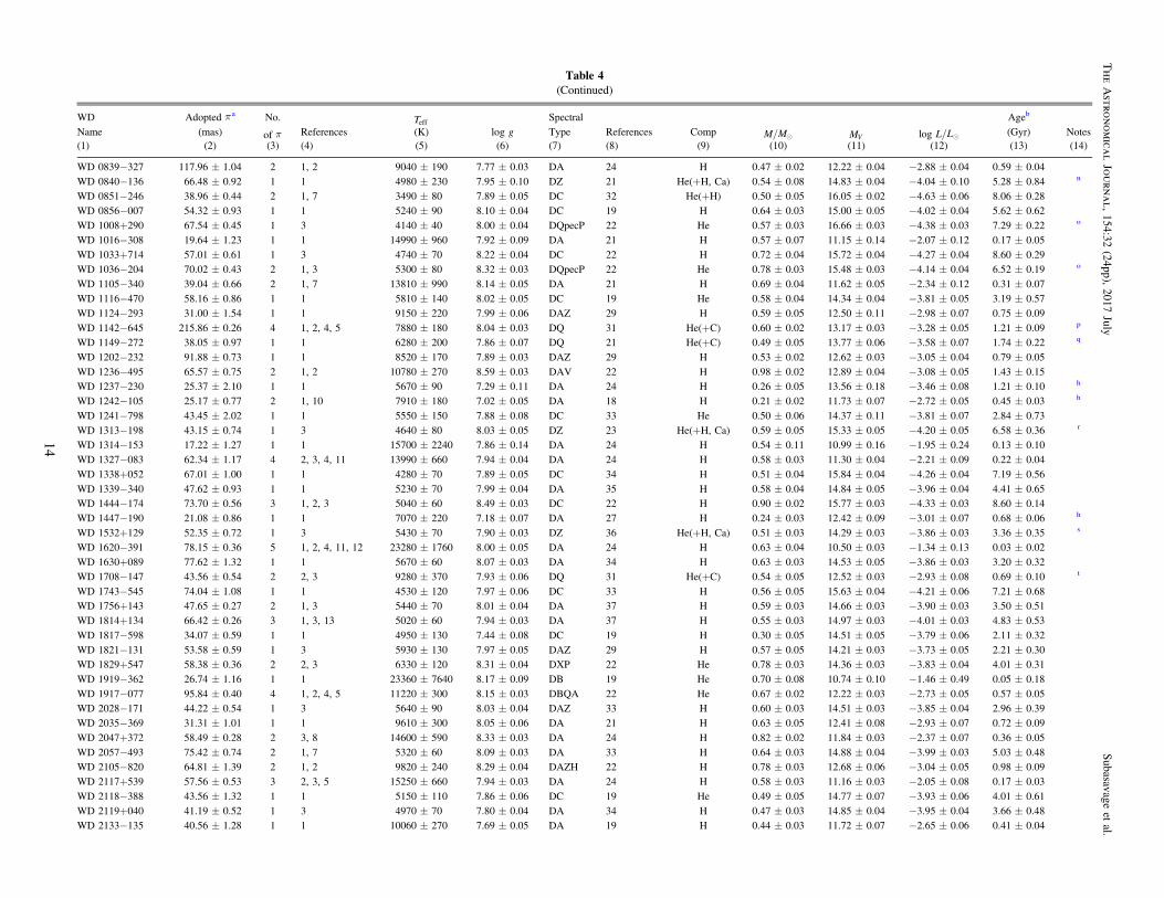
Table 4(Continued)

WD Adopted pa No. Teff Spectral Ageb

Name (mas) of p References (K) log g Type References Comp M/ M MV log L/ L (Gyr) Notes(1) (2) (3) (4) (5) (6) (7) (8) (9) (10) (11) (12) (13) (14)

WD 0839−327 117.96±1.04 2 1, 2 9040±190 7.77±0.03 DA 24 H 0.47±0.02 12.22±0.04 −2.88±0.04 0.59±0.04

WD 0840−136 66.48±0.92 1 1 4980±230 7.95±0.10 DZ 21 He(+H, Ca) 0.54±0.08 14.83±0.04 −4.04±0.10 5.28±0.84 n

WD 0851−246 38.96±0.44 2 1, 7 3490±80 7.89±0.05 DC 32 He(+H) 0.50±0.05 16.05±0.02 −4.63±0.06 8.06±0.28WD 0856−007 54.32±0.93 1 1 5240±90 8.10±0.04 DC 19 H 0.64±0.03 15.00±0.05 −4.02±0.04 5.62±0.62

WD 1008+290 67.54±0.45 1 3 4140±40 8.00±0.04 DQpecP 22 He 0.57±0.03 16.66±0.03 −4.38±0.03 7.29±0.22 o

WD 1016−308 19.64±1.23 1 1 14990±960 7.92±0.09 DA 21 H 0.57±0.07 11.15±0.14 −2.07±0.12 0.17±0.05

WD 1033+714 57.01±0.61 1 3 4740±70 8.22±0.04 DC 22 H 0.72±0.04 15.72±0.04 −4.27±0.04 8.60±0.29WD 1036−204 70.02±0.43 2 1, 3 5300±80 8.32±0.03 DQpecP 22 He 0.78±0.03 15.48±0.03 −4.14±0.04 6.52±0.19 o

WD 1105−340 39.04±0.66 2 1, 7 13810±990 8.14±0.05 DA 21 H 0.69±0.04 11.62±0.05 −2.34±0.12 0.31±0.07

WD 1116−470 58.16±0.86 1 1 5810±140 8.02±0.05 DC 19 He 0.58±0.04 14.34±0.04 −3.81±0.05 3.19±0.57

WD 1124−293 31.00±1.54 1 1 9150±220 7.99±0.06 DAZ 29 H 0.59±0.05 12.50±0.11 −2.98±0.07 0.75±0.09

WD 1142−645 215.86±0.26 4 1, 2, 4, 5 7880±180 8.04±0.03 DQ 31 He(+C) 0.60±0.02 13.17±0.03 −3.28±0.05 1.21±0.09 p

WD 1149−272 38.05±0.97 1 1 6280±200 7.86±0.07 DQ 21 He(+C) 0.49±0.05 13.77±0.06 −3.58±0.07 1.74±0.22 q

WD 1202−232 91.88±0.73 1 1 8520±170 7.89±0.03 DAZ 29 H 0.53±0.02 12.62±0.03 −3.05±0.04 0.79±0.05

WD 1236−495 65.57±0.75 2 1, 2 10780±270 8.59±0.03 DAV 22 H 0.98±0.02 12.89±0.04 −3.08±0.05 1.43±0.15WD 1237−230 25.37±2.10 1 1 5670±90 7.29±0.11 DA 24 H 0.26±0.05 13.56±0.18 −3.46±0.08 1.21±0.10 h

WD 1242−105 25.17±0.77 2 1, 10 7910±180 7.02±0.05 DA 18 H 0.21±0.02 11.73±0.07 −2.72±0.05 0.45±0.03 h

WD 1241−798 43.45±2.02 1 1 5550±150 7.88±0.08 DC 33 He 0.50±0.06 14.37±0.11 −3.81±0.07 2.84±0.73

WD 1313−198 43.15±0.74 1 3 4640±80 8.03±0.05 DZ 23 He(+H, Ca) 0.59±0.05 15.33±0.05 −4.20±0.05 6.58±0.36 r

WD 1314−153 17.22±1.27 1 1 15700±2240 7.86±0.14 DA 24 H 0.54±0.11 10.99±0.16 −1.95±0.24 0.13±0.10

WD 1327−083 62.34±1.17 4 2, 3, 4, 11 13990±660 7.94±0.04 DA 24 H 0.58±0.03 11.30±0.04 −2.21±0.09 0.22±0.04

WD 1338+052 67.01±1.00 1 1 4280±70 7.89±0.05 DC 34 H 0.51±0.04 15.84±0.04 −4.26±0.04 7.19±0.56

WD 1339−340 47.62±0.93 1 1 5230±70 7.99±0.04 DA 35 H 0.58±0.04 14.84±0.05 −3.96±0.04 4.41±0.65WD 1444−174 73.70±0.56 3 1, 2, 3 5040±60 8.49±0.03 DC 22 H 0.90±0.02 15.77±0.03 −4.33±0.03 8.60±0.14

WD 1447−190 21.08±0.86 1 1 7070±220 7.18±0.07 DA 27 H 0.24±0.03 12.42±0.09 −3.01±0.07 0.68±0.06 h

WD 1532+129 52.35±0.72 1 3 5430±70 7.90±0.03 DZ 36 He(+H, Ca) 0.51±0.03 14.29±0.03 −3.86±0.03 3.36±0.35 s

WD 1620−391 78.15±0.36 5 1, 2, 4, 11, 12 23280±1760 8.00±0.05 DA 24 H 0.63±0.04 10.50±0.03 −1.34±0.13 0.03±0.02

WD 1630+089 77.62±1.32 1 1 5670±60 8.07±0.03 DA 34 H 0.63±0.03 14.53±0.05 −3.86±0.03 3.20±0.32

WD 1708−147 43.56±0.54 2 2, 3 9280±370 7.93±0.06 DQ 31 He(+C) 0.54±0.05 12.52±0.03 −2.93±0.08 0.69±0.10 t

WD 1743−545 74.04±1.08 1 1 4530±120 7.97±0.06 DC 33 H 0.56±0.05 15.63±0.04 −4.21±0.06 7.21±0.68WD 1756+143 47.65±0.27 2 1, 3 5440±70 8.01±0.04 DA 37 H 0.59±0.03 14.66±0.03 −3.90±0.03 3.50±0.51

WD 1814+134 66.42±0.26 3 1, 3, 13 5020±60 7.94±0.03 DA 37 H 0.55±0.03 14.97±0.03 −4.01±0.03 4.83±0.53

WD 1817−598 34.07±0.59 1 1 4950±130 7.44±0.08 DC 19 H 0.30±0.05 14.51±0.05 −3.79±0.06 2.11±0.32

WD 1821−131 53.58±0.59 1 3 5930±130 7.97±0.05 DAZ 29 H 0.57±0.05 14.21±0.03 −3.73±0.05 2.21±0.30WD 1829+547 58.38±0.36 2 2, 3 6330±120 8.31±0.04 DXP 22 He 0.78±0.03 14.36±0.03 −3.83±0.04 4.01±0.31

WD 1919−362 26.74±1.16 1 1 23360±7640 8.17±0.09 DB 19 He 0.70±0.08 10.74±0.10 −1.46±0.49 0.05±0.18

WD 1917−077 95.84±0.40 4 1, 2, 4, 5 11220±300 8.15±0.03 DBQA 22 He 0.67±0.02 12.22±0.03 −2.73±0.05 0.57±0.05WD 2028−171 44.22±0.54 1 3 5640±90 8.03±0.04 DAZ 33 H 0.60±0.03 14.51±0.03 −3.85±0.04 2.96±0.39

WD 2035−369 31.31±1.01 1 1 9610±300 8.05±0.06 DA 21 H 0.63±0.05 12.41±0.08 −2.93±0.07 0.72±0.09

WD 2047+372 58.49±0.28 2 3, 8 14600±590 8.33±0.03 DA 24 H 0.82±0.02 11.84±0.03 −2.37±0.07 0.36±0.05

WD 2057−493 75.42±0.74 2 1, 7 5320±60 8.09±0.03 DA 33 H 0.64±0.03 14.88±0.04 −3.99±0.03 5.03±0.48WD 2105−820 64.81±1.39 2 1, 2 9820±240 8.29±0.04 DAZH 22 H 0.78±0.03 12.68±0.06 −3.04±0.05 0.98±0.09

WD 2117+539 57.56±0.53 3 2, 3, 5 15250±660 7.94±0.03 DA 24 H 0.58±0.03 11.16±0.03 −2.05±0.08 0.17±0.03

WD 2118−388 43.56±1.32 1 1 5150±110 7.86±0.06 DC 19 He 0.49±0.05 14.77±0.07 −3.93±0.06 4.01±0.61

WD 2119+040 41.19±0.52 1 3 4970±70 7.80±0.04 DA 34 H 0.47±0.03 14.85±0.04 −3.95±0.04 3.66±0.48WD 2133−135 40.56±1.28 1 1 10060±270 7.69±0.05 DA 19 H 0.44±0.03 11.72±0.07 −2.65±0.06 0.41±0.04

14

TheAstro

nomica

lJourn

al,

154:32(24pp),

2017July

Subasavage

etal.

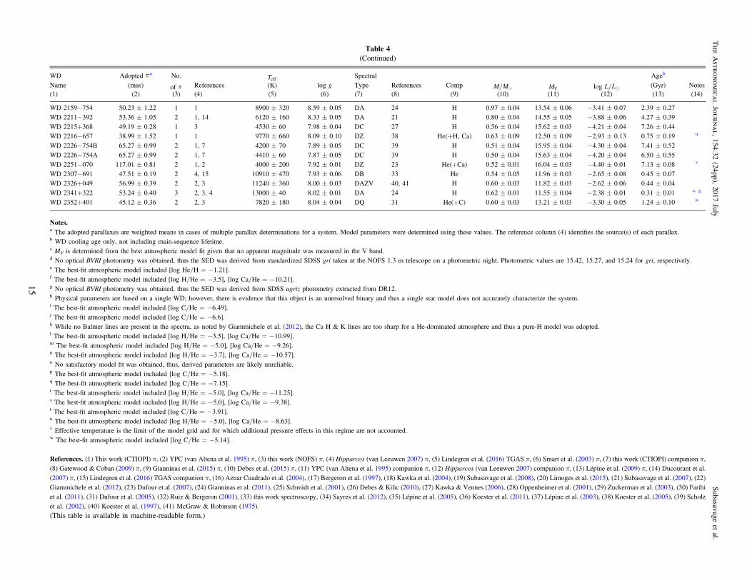
Table 4(Continued)

WD Adopted pa No. Teff Spectral Ageb

Name (mas) of p References (K) log g Type References Comp M/ M MV log L/ L (Gyr) Notes(1) (2) (3) (4) (5) (6) (7) (8) (9) (10) (11) (12) (13) (14)

WD 2159−754 50.23±1.22 1 1 8900±320 8.59±0.05 DA 24 H 0.97±0.04 13.54±0.06 −3.41±0.07 2.39±0.27

WD 2211−392 53.36±1.05 2 1, 14 6120±160 8.33±0.05 DA 21 H 0.80±0.04 14.55±0.05 −3.88±0.06 4.27±0.39

WD 2215+368 49.19±0.28 1 3 4530±60 7.98±0.04 DC 27 H 0.56±0.04 15.62±0.03 −4.21±0.04 7.26±0.44WD 2216−657 38.99±1.52 1 1 9770±660 8.09±0.10 DZ 38 He(+H, Ca) 0.63±0.09 12.50±0.09 −2.93±0.13 0.75±0.19 u

WD 2226−754B 65.27±0.99 2 1, 7 4200±70 7.89±0.05 DC 39 H 0.51±0.04 15.95±0.04 −4.30±0.04 7.41±0.52

WD 2226−754A 65.27±0.99 2 1, 7 4410±60 7.87±0.05 DC 39 H 0.50±0.04 15.63±0.04 −4.20±0.04 6.50±0.55WD 2251−070 117.01±0.81 2 1, 2 4000±200 7.92±0.01 DZ 23 He(+Ca) 0.52±0.01 16.04±0.03 −4.40±0.01 7.13±0.08 v

WD 2307−691 47.51±0.19 2 4, 15 10910±470 7.93±0.06 DB 33 He 0.54±0.05 11.96±0.03 −2.65±0.08 0.45±0.07

WD 2326+049 56.99±0.39 2 2, 3 11240±360 8.00±0.03 DAZV 40, 41 H 0.60±0.03 11.82±0.03 −2.62±0.06 0.44±0.04

WD 2341+322 53.24±0.40 3 2, 3, 4 13000±40 8.02±0.01 DA 24 H 0.62±0.01 11.55±0.04 −2.38±0.01 0.31±0.01 c, g

WD 2352+401 45.12±0.36 2 2, 3 7820±180 8.04±0.04 DQ 31 He(+C) 0.60±0.03 13.21±0.03 −3.30±0.05 1.24±0.10 w

Notes.a The adopted parallaxes are weighted means in cases of multiple parallax determinations for a system. Model parameters were determined using these values. The referencecolumn (4) identifies the source(s) of each parallax.b WD cooling age only, not including main-sequence lifetime.c MV is determined from the best atmospheric model fit given that no apparent magnitude was measured in the Vband.d No optical BVRI photometry was obtained, thus the SED was derived from standardized SDSS gri taken at the NOFS 1.3 m telescope on a photometric night. Photometric values are 15.42, 15.27, and 15.24 for gri, respectively.e The best-fit atmospheric model included [log He/H=−1.21].f The best-fit atmospheric model included [log H/He=−3.5], [log Ca/He=−10.21].g No optical BVRI photometry was obtained, thusthe SED was derived from SDSS ugriz photometry extracted from DR12.h Physical parameters are based on a single WD; however, there is evidence that this object is an unresolved binary and thusa single star model does not accurately characterize the system.i The best-fit atmospheric model included [log C/He=−6.49].j The best-fit atmospheric model included [log C/He=−6.6].k While no Balmer lines are present in the spectra, as notedby Giammichele et al. (2012), the Ca H & K lines are too sharp for a He-dominated atmosphere and thusa pure-H model was adopted.l The best-fit atmospheric model included [log H/He=−3.5], [log Ca/He=−10.99].m The best-fit atmospheric model included [log H/He=−5.0], [log Ca/He=−9.26].n The best-fit atmospheric model included [log H/He=−3.7], [log Ca/He=−10.57].o No satisfactory model fit was obtained, thus,derived parameters are likely unreliable.p The best-fit atmospheric model included [log C/He=−5.18].q The best-fit atmospheric model included [log C/He=−7.15].r The best-fit atmospheric model included [log H/He=−5.0], [log Ca/He=−11.25].s The best-fit atmospheric model included [log H/He=−5.0], [log Ca/He=−9.38].t The best-fit atmospheric model included [log C/He=−3.91].u The best-fit atmospheric model included [log H/He=−5.0], [log Ca/He=−8.63].v Effective temperature is the limit of the model grid and for which additional pressure effects in this regime are not accounted.w The best-fit atmospheric model included [log C/He=−5.14].

References. (1) This work (CTIOPI) π, (2) YPC (van Altena et al. 1995) π, (3) this work (NOFS) π, (4) Hipparcos (van Leeuwen 2007) π, (5) Lindegren et al. (2016) TGAS π, (6) Smart et al. (2003) π, (7) this work (CTIOPI) companion π,

(8) Gatewood & Coban (2009) π, (9) Gianninas et al. (2015) π, (10) Debes et al. (2015) π, (11) YPC (van Altena et al. 1995) companion π, (12) Hipparcos (van Leeuwen 2007) companion π, (13) Lépine et al. (2009) π, (14) Ducourant et al.(2007) π, (15) Lindegren et al. (2016) TGAS companion π, (16) Aznar Cuadrado et al. (2004), (17) Bergeron et al. (1997), (18) Kawka et al. (2004), (19) Subasavage et al. (2008), (20) Limoges et al. (2015), (21) Subasavage et al. (2007), (22)Giammichele et al. (2012), (23) Dufour et al. (2007), (24) Gianninas et al. (2011), (25) Schmidt et al. (2001), (26) Debes & Kilic (2010), (27) Kawka & Vennes (2006), (28) Oppenheimer et al. (2001), (29) Zuckerman et al. (2003), (30) Farihiet al. (2011), (31) Dufour et al. (2005), (32) Ruiz & Bergeron (2001), (33) this work spectroscopy, (34) Sayres et al. (2012), (35) Lépine et al. (2005), (36) Koester et al. (2011), (37) Lépine et al. (2003), (38) Koester et al. (2005), (39) Scholzet al. (2002), (40) Koester et al. (1997), (41) McGraw & Robinson (1975).(This table is available in machine-readable form.)

15

TheAstro

nomica

lJourn

al,

154:32(24pp),

2017July

Subasavage

etal.

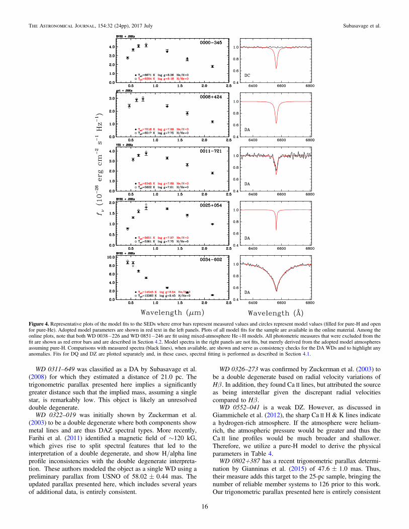
WD 0311–649 was classified as a DA by Subasavage et al.(2008) for which they estimated a distance of 21.0 pc. Thetrigonometric parallax presented here implies a significantlygreater distance such that the implied mass, assuming a singlestar, is remarkably low. This object is likely an unresolveddouble degenerate.

WD 0322–019 was initially shown by Zuckerman et al.(2003) to be a double degenerate where both components showmetal lines and are thus DAZ spectral types. More recently,Farihi et al. (2011) identifieda magnetic field of ∼120 kG,which gives rise to split spectral features that led to theinterpretation of a double degenerate, and show H/alpha lineprofile inconsistencies with the double degenerate interpreta-tion. These authors modeled the object as a single WD using apreliminary parallax from USNO of 58.02±0.44 mas. Theupdated parallax presented here, which includes several yearsof additional data, is entirely consistent.

WD 0326–273 was confirmed by Zuckerman et al. (2003) tobe a double degenerate based on radial velocity variations ofbH . In addition, they found Ca II lines, but attributed the source

as being interstellar given the discrepant radial velocitiescompared to bH .WD 0552–041 is a weak DZ. However, as discussed in

Giammichele et al. (2012), the sharp Ca II H & K lines indicatea hydrogen-rich atmosphere. If the atmosphere were helium-rich, the atmospheric pressure would be greaterand thus theCa II line profiles would be much broader and shallower.Therefore, we utilize a pure-H model to derive the physicalparameters in Table 4.WD 0802+387 has a recent trigonometric parallax determi-

nation by Gianninas et al. (2015) of 47.6±1.0 mas. Thus,their measure adds this target to the 25-pc sample, bringing thenumber of reliable member systems to 126 prior to this work.Our trigonometric parallax presented here is entirely consistent

Figure 4. Representative plots of the model fits to the SEDs where error bars represent measured values and circles represent model values (filled for pure-H and openfor pure-He). Adopted model parameters are shown in red text in the left panels. Plots of all model fits for the sample are available in the online material. Among theonline plots, note that both WD 0038−226 and WD 0851−246 are fit using mixed-atmosphere He+H models. All photometric measures that were excluded from thefit are shown as red error bars and aredescribed in Section 4.2. Model spectra in the right panels are not fits, but merely derived from the adopted model atmospheresassuming pure-H. Comparisons with measured spectra (black lines), when available, are shown and serve as consistency checks for the DA WDs and to highlight anyanomalies. Fits for DQ and DZ are plotted separately and, in these cases, spectral fitting is performed as described in Section 4.1.

16

The Astronomical Journal, 154:32 (24pp), 2017 July Subasavage et al.

and is included in our number counts as an updated measure.The weighted mean of these two measures is used to calculatephysical parameters shown in Table 4.

WD 0851–246 was first discovered to be a high proper-motionstar by Luyten (1974; LP 844−26; LHS 2068, Luyten 1979b)with μ=0 630 yr−1 at position angle 78 .0. It has a commonproper-motion companion (LHS 2067) whose spectral type islisted as sdM in Kirkpatrick et al. (1995). The WD componentwas first spectroscopically identified by Ruiz & Bergeron(2001), named CE 51 by those authorsduring a follow-upspectroscopic campaign targeting proper-motion objects detectedin the Calán-ESO survey (Ruiz et al. 2001). They determinedthat the WD is very cool (2730 K), old (11.9 Gyr), and nearby(14.7±0.3 pc). Silvestri et al. (2002) conducted a radialvelocity survey of wide binaries with WD components,including this system, and found a = V 0.0 15.8rad km s−1

for the sdM. Based on the WD’s location in the H–R diagram(Figure 3), it is expected that CIA is present and likely resultsfrom collisions with molecular helium andthusis a mixed-atmosphere He+H. The physical parameters presented inTable 4 are derived from a mixed-atmosphere model with thefit shown in Figure 4. This is the coolest WD presented here forwhich we were able to derive reliable atmospheric parameters.Notably, the mixed-atmosphere fits results in a significantlyhigher Teff (3490 K) than that found by Ruiz & Bergeron (2001).

Additionally, Kilic et al. (2009) observed this system withSpitzer in the IRAC bandpasses, but stated that contaminationfrom a nearby bright star makes the photometry questionable.As discussed in Section 2.1.2, we obtained JHKs photometryusing NEWFIRM on the CTIO Blanco 4 m. The SED clearlyshows excess in the near-IR indicative of a cool, very redtertiary companion. Follow-up observations, in particular, near-IR spectroscopy, are required to characterize the tertiarycompanion. The mixed-atmosphere fit shown in Figure 4excludes the JHKs values; the optical magnitudes are notaffected by this very red unseen companion.

WD 1008+290 is a peculiar DQ WD with exceptional Swanband absorption such that the measured V magnitude, whosebandpass encompasses a portion of this absorption, is affectedand appears fainter than if the absorption was not present.Additionally, the V−I color is inflated for the same reasonresulting in the WD’s displacement in Figure 3. We adopt apure-He model atmosphere simply because there was nosatisfactory agreement with the SED, regardless of model used;thus, the atmospheric parameters are likely unreliable.

WD 1036–204 is another peculiar DQ WD with exceptionalSwan band absorption. We adopt a pure-He model atmospheresimply because there was no satisfactory agreement with theSED, regardless of model used, thus, the atmosphericparameters are likely unreliable.

WD 1237–230 was first discovered to be a high proper-motion star by Luyten (1972; LP 853−15; LHS 339, Luyten1979b) with μ=1 102 yr−1 at position angle 219 .9. It wasfirst classified as a DA WD by Liebert & Strittmatter (1977).Subasavage et al. (2007) obtained optical VRI photometry andcombined it with JHKS from 2MASS to model the SED andderive physical parameters. One significant discrepancy is thedistance estimate derived (26.9±4.5 pc) compared to thetrigonometric distance determined in this work (39.4±3.6 pc).The recent spectroscopic analysis of Kawka & Vennes (2012)showed this object to be a single-lined binaryand theyidentifiedthis object to be a candidate halo WD based on the

estimated distance. Our trigonometric parallax further strength-ens the case for halo membership, as it has an extremetangential velocity of 202.4 km s−1. We see no evidence forphotocentric motion in the astrometric data set, leaving opentwo possibilities: (1) a system with two roughly equal-mass,equal-luminosity componentsor (2) a system with a periodshort enough (P1 year) to evade detection in our astrometricdata. Given the overluminosity in the optical (see Figure 3),such that the components are of similar brightnesses, coupledwith the single-lined radial velocity variation, the system islikely composed of a DA and a non-DA pair of WDs.WD 1241–798 was classified as a DQ/DC by Subasavage

et al. (2008) without further explanation. The ambiguousspectral classification arises because the authors obtained a redspectrum from the Blanco 4 m at CTIO using the R-CSpectrograph. With a blue cutoff of ∼5500 Å, no sharp featureswere present, yet there were depressions very close to wherethe C2 Swan bands are expected but the detection is marginal.To remove this discrepancy, we acquired a confirmationspectrum using SOAR + Goodman during an engineeringnight on 2017.28 UT and as described in Section 2.2. Whileundulations exist in the spectrum, they correlate with theinternal quartz lamp used for flat fielding such that this object isof spectral type DC, as shown in Figure 1. This object is similarto WD 0000−345 in that a pure-H model better fits the SEDover a pure-He model, yet no Balmer features are seen in thespectrum. Thus, we use a pure-He atmospheric model tocharacterize this object.WD 1242–105 was first classified as a hot subdwarf (sdB) by

Kilkenny et al. (1988) and later identified as a DA WD byVennes & Kawka (2003), who estimated a photometricdistance of 18±4 pc. It was then placed on the parallaxprogram to confirm proximity. With a trigonometric parallaxdistance of -

+41.1 2.332.63 pc, we suspected this object to be an

unresolved double star.During a spectroscopic campaign using the SOAR telescope

with the Goodman spectrograph briefly described inSection 2.2, we were assisting with the commissioning of a2100 lines-per-mm VPH grating and chose to observe thisobject as a test case. The observations were taken on 2011 July22 and a slit width of 0 84 was used to optimize spectralresolution and throughput. Spectral coverage was 3700−4400 Åwith a spectral resolution of 0.8 Åpixel−1. The longslit was oriented so that a bright calibrator (2MASS J12445203−1049037) was also in the slit to serve as a check for anywavelength calibration systematic uncertainties (though it wasnot known a priori if this calibrator was radial velocity stable).The targets were observed for ∼2 hr, taking repeated exposuresof 150 s each. After every seven exposures, arc lamps weretaken to ensure accurate wavelength calibration. Spectroscopicreductions were performed using standard IRAF routines in theSpecred package. Once wavelength calibration was performedon each spectrum (using the arc lamp taken closest in time),each block of seven spectra was stacked to increase S/N, thusresulting in a cadence of roughly 25 minutes. For consistency,the calibrator spectra were stacked in an identical manner. SeeFigure 5.Once it was evident that the system was a double-lined

double degenerate with rapidly changing relative velocities, werequested the use of the Gemini Multi-object Spectrograph-south (GMOS-S) to better characterize the orbital period.Spectroscopic data were taken on 2012.31 UT using the

17

The Astronomical Journal, 154:32 (24pp), 2017 July Subasavage et al.

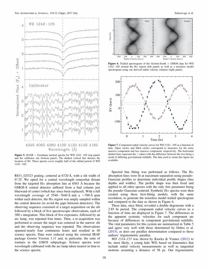
R831_G5323 grating, centered at 6720 Å, with a slit width of0 25. We opted for a central wavelength somewhat distantfrom the targeted Hα absorption line at 6563 Åbecause theGMOS-S central detector suffered from a bad column justblueward of center (which hassince been replaced). With a fullwavelength coverage of 5540−7640 Åand a ∼700 Åspanwithin each detector, the Hα region was amply sampled withinthe central detector (to avoid the gaps between detectors). Theobserving sequence consisted of a target acquisition on the slitfollowed by a block of five spectroscopic observations, each of300 s integration. This block of five exposures, followed by anarc lamp, was repeated four times. Then, a re-acquisition wasperformed to ensure the target was centered in the narrow slitand the observing sequence was repeated. The observationsspannednearly four continuous hours and resulted in 40science spectra. Data were reduced using the external IRAFpackage Gemini Version 1.11 and, in particular, the suite ofroutines in the GMOS subpackage. Science spectra werewavelength calibrated with the arc lamp taken nearest in time tothe science spectra.

Spectral line fitting was performed as follows. The Hαabsorption lines were fit at maximum separation using pseudo–Gaussian profiles to determine individual profile shapes (linedepths and widths). The profile shape was then fixed andapplied to all other spectra with the only free parameter beingthe pseudo–Gaussian centroid. Synthetic Hα spectra were thencreated using these best-fitting models, with the sameresolution, to generate the noiseless model trailed spectrogramand compared to the data as shown in Figure 6.These data, once fitted, revealed a double degenerate with a

2.85 hr period. The component radial velocity curves as afunction of time are displayed in Figure 7. The differences inthe apparent systemic velocities for each component arebecause of differences in component gravitational redshifts.The vital parameters for this system are summarized in Table 5and agree very well with those determined by Debes et al.(2015), as does our parallax determination compared to thoseauthors’ trigonometric parallax.WD 1314–153 was shownby Kawka & Vennes (2012) to

be, most likely, a young halo WD,based on kinematics thatinclude radial velocity measurements as well as tangentialmotions assuming a distance of 58 pc. Our trigonometric

Figure 5. SOAR + Goodman stacked spectra for WD 1242−105 (top panel)and the calibrator star (bottom panel). The dashed vertical line denotes thelocation of Hδ. These spectra cover roughly half of the orbital period of WD1242−105.

Figure 6. Trailed spectrogram of the Gemini-South + GMOS data for WD1242−105 around the Hα region (left panel) as well as a noiseless modelspectrogram using our derived radial velocity solution (right panel).

Figure 7. Component radial velocity curves for WD 1242−105 as a function oftime. Open circles and filled circles correspond to measures for the moremassive component and less massive component, respectively. The horizontaldashed lines represent the γ values with the difference between the two being aresult of differing gravitational redshifts. The data used to create this figure areavailable.

18

The Astronomical Journal, 154:32 (24pp), 2017 July Subasavage et al.

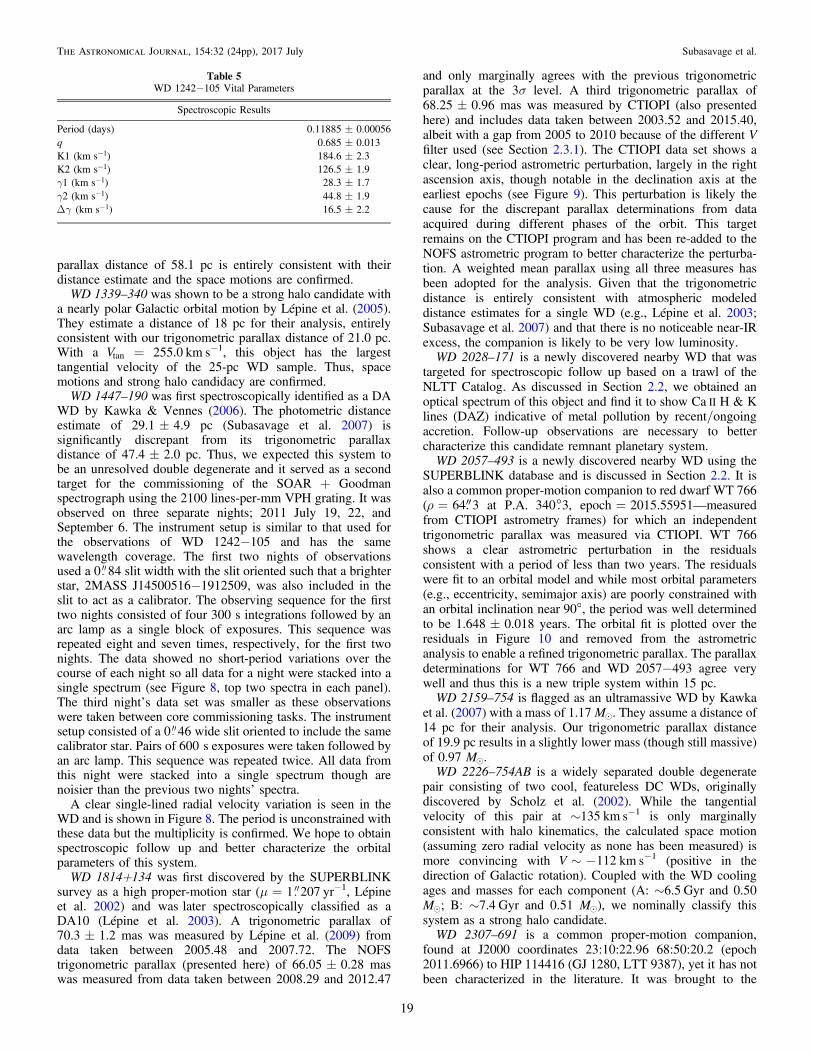
parallax distance of 58.1 pc is entirely consistent with theirdistance estimate and the space motions are confirmed.

WD 1339–340 was shown to be a strong halo candidate witha nearly polar Galactic orbital motion by Lépine et al. (2005).They estimate a distance of 18 pc for their analysis, entirelyconsistent with our trigonometric parallax distance of 21.0 pc.With a Vtan = 255.0 km s−1, this object has the largesttangential velocity of the 25-pc WD sample. Thus, spacemotions and strong halo candidacy are confirmed.

WD 1447–190 was first spectroscopically identified as a DAWD by Kawka & Vennes (2006). The photometric distanceestimate of 29.1±4.9 pc (Subasavage et al. 2007) issignificantly discrepant from its trigonometric parallaxdistance of 47.4±2.0 pc. Thus, we expected this system tobe an unresolved double degenerate and it served as a secondtarget for the commissioning of the SOAR + Goodmanspectrograph using the 2100 lines-per-mm VPH grating. It wasobserved on three separate nights; 2011 July 19, 22, andSeptember 6. The instrument setup is similar to that used forthe observations of WD 1242−105 and has the samewavelength coverage. The first two nights of observationsused a 0 84 slit width with the slit oriented such that a brighterstar, 2MASS J14500516−1912509, was also included in theslit to act as a calibrator. The observing sequence for the firsttwo nights consisted of four 300s integrations followed by anarc lamp as a single block of exposures. This sequence wasrepeated eightand seven times, respectively, for the first twonights. The data showed no short-period variations over thecourse of each night so all data for a night were stacked into asingle spectrum (see Figure 8, top two spectra in each panel).The third night’s data set was smaller as these observationswere taken between core commissioning tasks. The instrumentsetup consisted of a 0 46 wide slit oriented to include the samecalibrator star. Pairs of 600s exposures were taken followed byan arc lamp. This sequence was repeated twice. All data fromthis night were stacked into a single spectrum though arenoisier than the previous two nights’ spectra.

A clear single-lined radial velocity variation is seen in theWD and is shown in Figure 8. The period is unconstrained withthese data but the multiplicity is confirmed. We hope to obtainspectroscopic follow up and better characterize the orbitalparameters of this system.

WD 1814+134 was first discovered by the SUPERBLINKsurvey as a high proper-motion star (μ=1 207 yr−1, Lépineet al. 2002) and waslater spectroscopically classified as aDA10 (Lépine et al. 2003). A trigonometric parallax of70.3±1.2 mas was measured by Lépine et al. (2009) fromdata taken between 2005.48 and 2007.72. The NOFStrigonometric parallax (presented here) of 66.05±0.28 maswas measured from data taken between 2008.29 and 2012.47

and only marginally agrees with the previous trigonometricparallax at the 3σ level. A third trigonometric parallax of68.25±0.96 mas was measured by CTIOPI (also presentedhere) and includes data taken between 2003.52 and 2015.40,albeit with a gap from 2005 to 2010 because of the different Vfilter used (see Section 2.3.1). The CTIOPI data set shows aclear, long-period astrometric perturbation, largely in the rightascension axis, though notable in the declination axis at theearliest epochs (see Figure 9). This perturbation is likely thecause for the discrepant parallax determinations from dataacquired during different phases of the orbit. This targetremains on the CTIOPI programand has been re-added to theNOFS astrometric program to better characterize the perturba-tion. A weighted mean parallax using all three measures hasbeen adopted for the analysis. Given that the trigonometricdistance is entirely consistent with atmospheric modeleddistance estimates for a single WD (e.g., Lépine et al. 2003;Subasavage et al. 2007)and thatthere is no noticeable near-IRexcess, the companion is likely to be very lowluminosity.WD 2028–171 is a newly discovered nearby WD that was

targeted for spectroscopic follow up based on a trawl of theNLTT Catalog. As discussed in Section 2.2, we obtained anoptical spectrum of this object and find it to show Ca II H & Klines (DAZ) indicative of metal pollution by recent/ongoingaccretion. Follow-up observations are necessary to bettercharacterize this candidate remnant planetary system.WD 2057–493 is a newly discovered nearby WD using the

SUPERBLINK database and is discussed in Section 2.2. It isalso a common proper-motion companion to red dwarf WT 766(r = 64. 3 at P.A. 340 .3, epoch=2015.55951—measuredfrom CTIOPI astrometry frames) for which an independenttrigonometric parallax was measured via CTIOPI. WT 766shows a clear astrometric perturbation in the residualsconsistent with a period of less than two years. The residualswere fit to an orbital modeland while most orbital parameters(e.g., eccentricity, semimajor axis) are poorly constrained withan orbital inclination near 90 , the period was well determinedto be 1.648±0.018 years. The orbital fit is plotted over theresiduals in Figure 10 and removed from the astrometricanalysis to enable a refined trigonometric parallax. The parallaxdeterminations for WT 766 and WD 2057−493 agree verywelland thus this is a new triple system within 15 pc.WD 2159–754 is flagged as an ultramassive WD by Kawka

et al. (2007) with a mass of 1.17 M . They assume a distance of14 pc for their analysis. Our trigonometric parallax distanceof 19.9 pc results in a slightly lower mass (though still massive)of 0.97 M .WD 2226–754AB is a widely separated double degenerate

pair consisting of two cool, featureless DC WDs, originallydiscovered by Scholz et al. (2002). While the tangentialvelocity of this pair at ∼135 km s−1 is only marginallyconsistent with halo kinematics, the calculated space motion(assuming zero radial velocity as none has been measured) ismore convincing with ~ -V 112 km s−1 (positive in thedirection of Galactic rotation). Coupled with the WD coolingages and masses for each component (A: ∼6.5 Gyr and 0.50M ; B: ∼7.4 Gyr and 0.51 M ), we nominally classify this

system as a strong halo candidate.WD 2307–691 is a common proper-motion companion,

found at J2000 coordinates 23:10:22.96 68:50:20.2 (epoch2011.6966) to HIP 114416 (GJ 1280, LTT 9387), yet ithas notbeen characterized in the literature. It was brought to the

Table 5WD 1242−105 Vital Parameters

Spectroscopic Results

Period (days) 0.11885±0.00056q 0.685±0.013K1 (km -s 1) 184.6±2.3K2 (km -s 1) 126.5±1.9γ1 (km -s 1) 28.3±1.7γ2 (km -s 1) 44.8±1.9gD (km -s 1) 16.5±2.2

19

The Astronomical Journal, 154:32 (24pp), 2017 July Subasavage et al.

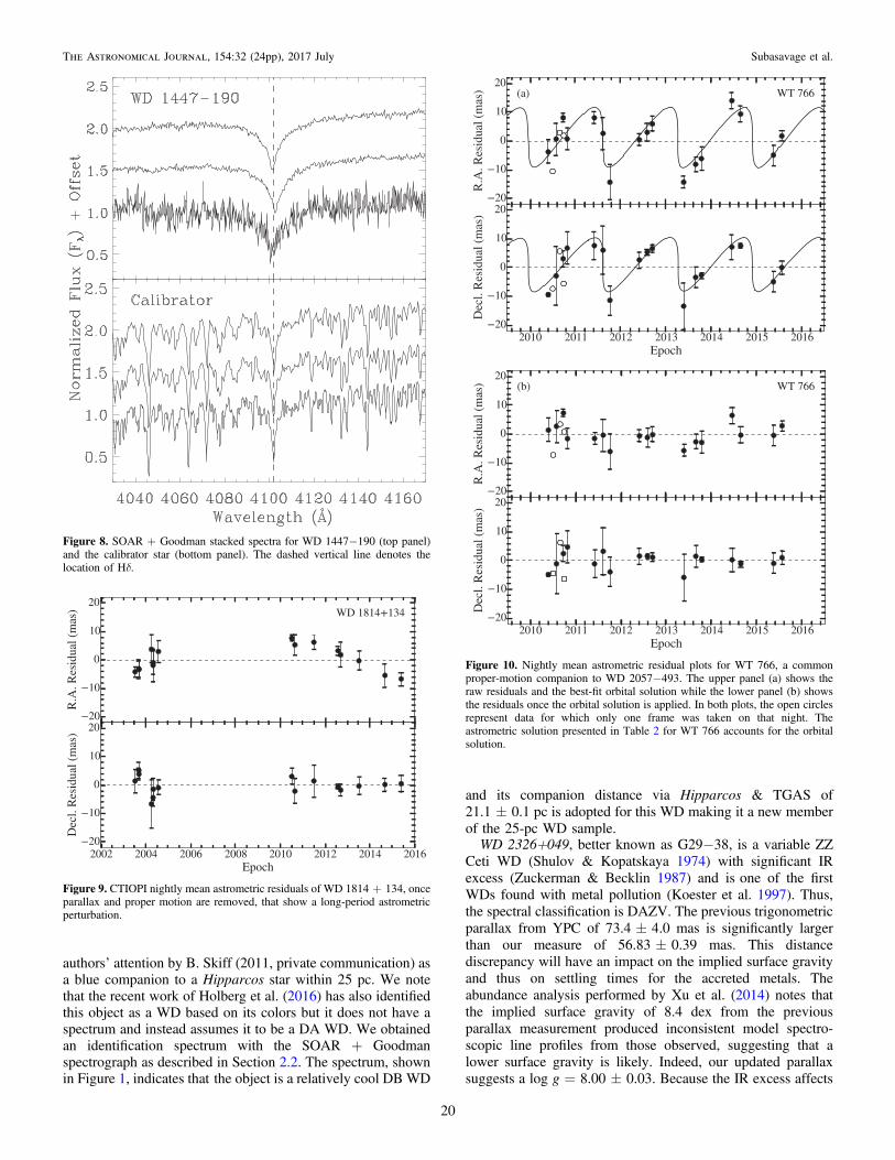
authors’ attention by B. Skiff (2011, private communication) asa blue companion to a Hipparcos star within 25 pc. We notethat the recent work of Holberg et al. (2016) has also identifiedthis object as a WD based on its colors but it does not have aspectrum and instead assumes it to be a DA WD. We obtainedan identification spectrum with the SOAR + Goodmanspectrograph as described in Section 2.2. The spectrum, shownin Figure 1, indicates thatthe object is a relatively cool DB WD

and its companion distance via Hipparcos & TGAS of21.1±0.1 pc is adopted for this WD making it a new memberof the 25-pc WD sample.WD 2326+049, better known as G29−38, is a variable ZZ

Ceti WD (Shulov & Kopatskaya 1974) with significant IRexcess (Zuckerman & Becklin 1987) and isone of the firstWDs found with metal pollution (Koester et al. 1997). Thus,the spectral classification is DAZV. The previous trigonometricparallax from YPC of 73.4±4.0 mas is significantly largerthan our measure of 56.83±0.39 mas. This distancediscrepancy will have an impact on the implied surface gravityand thus on settling times for the accreted metals. Theabundance analysis performed by Xu et al. (2014) notes thatthe implied surface gravity of 8.4 dex from the previousparallax measurement produced inconsistent model spectro-scopic line profiles from those observed, suggesting that alower surface gravity is likely. Indeed, our updated parallaxsuggests a log g=8.00±0.03. Because the IR excess affects

Figure 8. SOAR + Goodman stacked spectra for WD 1447−190 (top panel)and the calibrator star (bottom panel). The dashed vertical line denotes thelocation of Hδ.

Figure 9. CTIOPI nightly mean astrometric residuals of WD 1814+134, onceparallax and proper motion are removed, that show a long-period astrometricperturbation.

Figure 10. Nightly mean astrometric residual plots for WT 766, a commonproper-motion companion to WD 2057−493. The upper panel (a) shows theraw residuals and the best-fit orbital solution while the lower panel (b) showsthe residuals once the orbital solution is applied. In both plots, the open circlesrepresent data for which only one frame was taken on that night. Theastrometric solution presented in Table 2 for WT 766 accounts for the orbitalsolution.

20

The Astronomical Journal, 154:32 (24pp), 2017 July Subasavage et al.

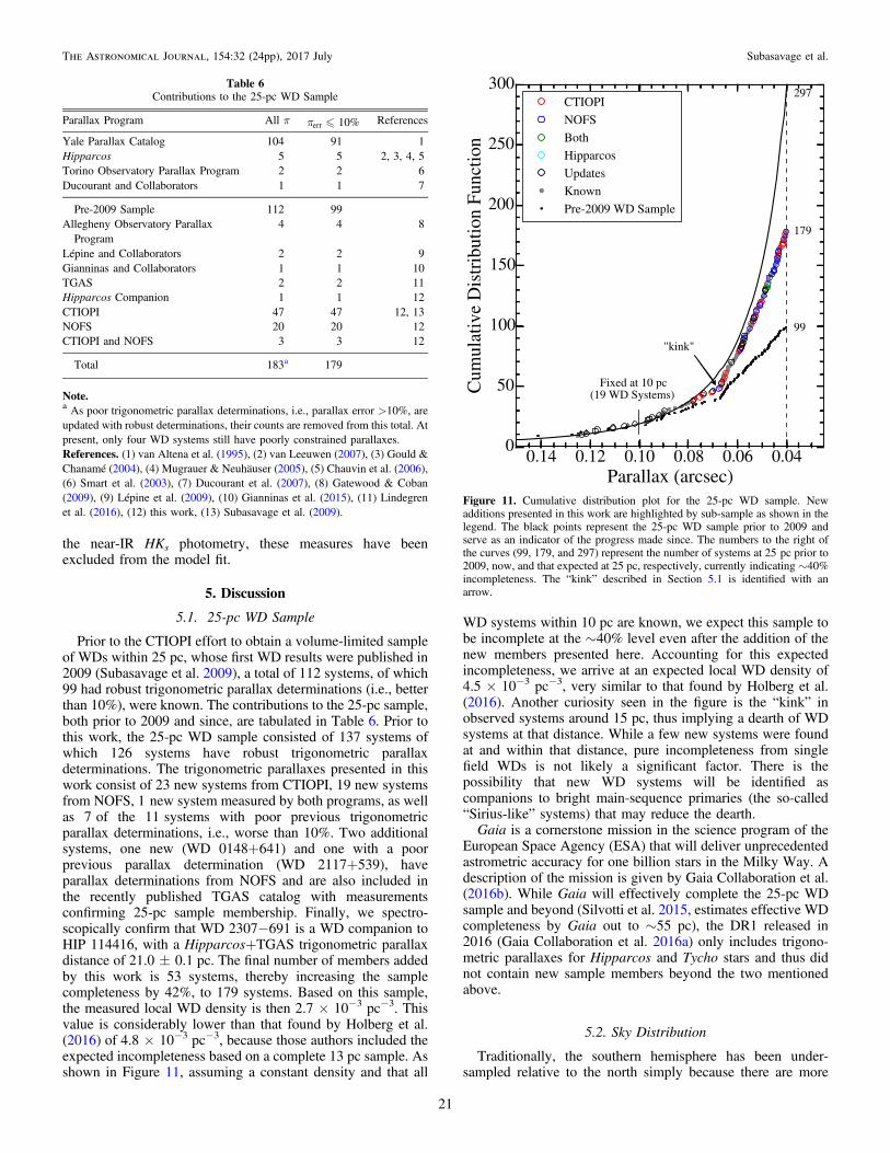
the near-IR HKs photometry, these measures have beenexcluded from the model fit.

5. Discussion

5.1. 25-pc WD Sample

Prior to the CTIOPI effort to obtain a volume-limited sampleof WDs within 25 pc, whose first WD results were published in2009 (Subasavage et al. 2009), a total of 112 systems, of which99 had robust trigonometric parallax determinations (i.e., betterthan 10%), were known. The contributions to the 25-pc sample,both prior to 2009 and since, are tabulated in Table 6. Prior tothis work, the 25-pc WD sample consisted of 137 systemsofwhich 126 systems have robust trigonometric parallaxdeterminations. The trigonometric parallaxes presented in thiswork consist of 23 new systems from CTIOPI, 19 new systemsfrom NOFS, 1new system measured by both programs, as wellas 7of the 11systems with poor previous trigonometricparallax determinations, i.e., worse than 10%. Two additionalsystems, one new (WD 0148+641) and one with a poorprevious parallax determination (WD 2117+539), haveparallax determinations from NOFS and are also included inthe recently published TGAS catalog with measurementsconfirming 25-pc sample membership. Finally, we spectro-scopically confirm that WD 2307−691 is a WD companion toHIP 114416, with a Hipparcos+TGAS trigonometric parallaxdistance of 21.0±0.1 pc. The final number of members addedby this work is 53 systems, thereby increasing the samplecompleteness by 42%, to 179 systems. Based on this sample,the measured local WD density is then 2.7×10−3 pc−3. Thisvalue is considerably lower than that found by Holberg et al.(2016) of 4.8×10−3 pc−3, because those authors included theexpected incompleteness based on a complete 13 pc sample. Asshown in Figure 11, assuming a constant density and that all

WD systems within 10 pc are known, we expect this sample tobe incomplete at the ∼40% level even after the addition of thenew members presented here. Accounting for this expectedincompleteness, we arrive at an expected local WD density of4.5×10−3 pc−3, very similar to that found by Holberg et al.(2016). Another curiosity seen in the figure is the “kink” inobserved systems around 15 pc, thus implying a dearth of WDsystems at that distance. While a few new systems were foundat and within that distance, pure incompleteness from singlefield WDs is not likely a significant factor. There is thepossibility that new WD systems will be identified ascompanions to bright main-sequence primaries (the so-called“Sirius-like” systems) that may reduce the dearth.Gaia is a cornerstone mission in the science programof the

European Space Agency (ESA) that will deliver unprecedentedastrometric accuracy for one billion stars in the Milky Way. Adescription of the mission is given by Gaia Collaboration et al.(2016b). While Gaia will effectively complete the 25-pc WDsample and beyond (Silvotti et al. 2015, estimates effective WDcompleteness by Gaia out to ∼55 pc), the DR1 released in2016 (Gaia Collaboration et al. 2016a) only includes trigono-metric parallaxes for Hipparcos and Tycho stars and thusdidnot contain new sample members beyond the two mentionedabove.

5.2. Sky Distribution

Traditionally, the southern hemisphere has been under-sampled relative to the north simply because there are more

Table 6Contributions to the 25-pc WD Sample

Parallax Program All π p 10%err References

Yale Parallax Catalog 104 91 1Hipparcos 5 5 2, 3, 4, 5Torino Observatory Parallax Program 2 2 6Ducourant and Collaborators 1 1 7

Pre-2009 Sample 112 99Allegheny Observatory Parallax

Program4 4 8

Lépine and Collaborators 2 2 9Gianninas and Collaborators 1 1 10TGAS 2 2 11Hipparcos Companion 1 1 12CTIOPI 47 47 12, 13NOFS 20 20 12CTIOPI and NOFS 3 3 12

Total 183a 179

Note.a As poor trigonometric parallax determinations, i.e., parallax error >10%, areupdated with robust determinations, their counts are removed from this total. Atpresent, only four WD systems still have poorly constrained parallaxes.References. (1) van Altena et al. (1995), (2) van Leeuwen (2007), (3) Gould &Chanamé (2004), (4) Mugrauer & Neuhäuser (2005), (5) Chauvin et al. (2006),(6) Smart et al. (2003), (7) Ducourant et al. (2007), (8) Gatewood & Coban(2009), (9) Lépine et al. (2009), (10) Gianninas et al. (2015), (11) Lindegrenet al. (2016), (12) this work, (13) Subasavage et al. (2009).

Figure 11. Cumulative distribution plot for the 25-pc WD sample. Newadditions presented in this work are highlighted by sub-sample as shown in thelegend. The black points represent the 25-pc WD sample prior to 2009 andserve as an indicator of the progress made since. The numbers to the right ofthe curves (99, 179, and 297) represent the number of systems at 25pc prior to2009, now, and that expected at 25 pc, respectively, currentlyindicating ∼40%incompleteness. The “kink” described in Section 5.1 is identified with anarrow.

21

The Astronomical Journal, 154:32 (24pp), 2017 July Subasavage et al.

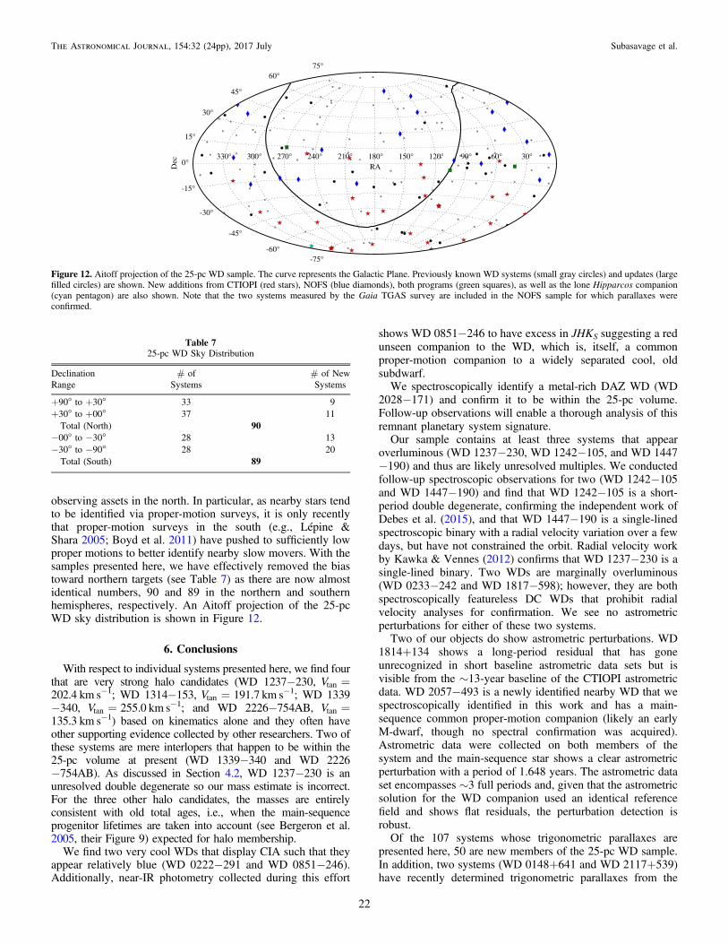
observing assets in the north. In particular, as nearby stars tendto be identified via proper-motion surveys, it is only recentlythat proper-motion surveys in the south (e.g., Lépine &Shara 2005; Boyd et al. 2011) have pushed to sufficiently lowproper motions to better identify nearbyslow movers. With thesamples presented here, we have effectively removed the biastoward northern targets (see Table 7) as there are now almostidentical numbers, 90 and 89 in the northern and southernhemispheres, respectively. An Aitoff projection of the 25-pcWD sky distribution is shown in Figure 12.

6. Conclusions

With respect to individual systems presented here, we find fourthat are very strong halo candidates (WD 1237−230, Vtan=202.4 km s−1; WD 1314−153, Vtan=191.7 km s−1; WD 1339−340, Vtan=255.0 km s−1; and WD 2226−754AB, Vtan=135.3 km s−1) based on kinematics alone and they often haveother supporting evidence collected by other researchers. Two ofthese systems are mere interlopers that happen to be within the25-pc volume at present (WD 1339−340 and WD 2226−754AB). As discussed in Section 4.2, WD 1237−230 is anunresolved double degenerate so our mass estimate is incorrect.For the three other halo candidates, the masses are entirelyconsistent with old total ages, i.e., when the main-sequenceprogenitor lifetimes are taken into account (see Bergeron et al.2005, their Figure 9) expected for halo membership.

We find two very cool WDs that display CIA such that theyappear relatively blue (WD 0222−291 and WD 0851−246).Additionally, near-IR photometry collected during this effort

shows WD 0851−246 to have excess in JHKS suggesting a redunseen companion to the WD, which is, itself, a commonproper-motion companion to a widely separated cool, oldsubdwarf.We spectroscopically identify a metal-rich DAZ WD (WD

2028−171) and confirm it to be within the 25-pc volume.Follow-up observations will enable a thorough analysis of thisremnant planetary system signature.Our sample contains at least three systems that appear

overluminous (WD 1237−230, WD 1242−105, and WD 1447−190) and thus are likely unresolved multiples. We conductedfollow-up spectroscopic observations for two (WD 1242−105and WD 1447−190) and find that WD 1242−105 is a short-period double degenerate, confirming the independent work ofDebes et al. (2015), and that WD 1447−190 is a single-linedspectroscopic binary with a radial velocity variation over a fewdays, but have not constrained the orbit. Radial velocity workby Kawka & Vennes (2012) confirms that WD 1237−230 is asingle-lined binary. Two WDs are marginally overluminous(WD 0233−242 and WD 1817−598); however, they are bothspectroscopically featureless DC WDs that prohibit radialvelocity analyses for confirmation. We see no astrometricperturbations for either of these two systems.Two of our objects do show astrometric perturbations. WD

1814+134 shows a long-period residual that has goneunrecognized in short baseline astrometric data sets but isvisible from the ∼13-year baseline of the CTIOPI astrometricdata. WD 2057−493 is a newly identified nearby WD that wespectroscopically identified in this work and has a main-sequence common proper-motion companion (likely an earlyM-dwarf, though no spectral confirmation was acquired).Astrometric data were collected on both members of thesystem and the main-sequence star shows a clear astrometricperturbation with a period of 1.648 years. The astrometric dataset encompasses ∼3 full periods and, given that the astrometricsolution for the WD companion used an identical referencefield and shows flat residuals, the perturbation detection isrobust.Of the 107 systems whose trigonometric parallaxes are

presented here, 50 are new members of the 25-pc WD sample.In addition, two systems (WD 0148+641 and WD 2117+539)have recently determined trigonometric parallaxes from the

Table 725-pc WD Sky Distribution

Declination # of # of NewRange Systems Systems

+90° to +30° 33 9+30° to +00° 37 11Total (North) 90−00° to −30° 28 13−30° to −90° 28 20Total (South) 89

Figure 12. Aitoff projection of the 25-pc WD sample. The curve represents the Galactic Plane. Previously known WD systems (small gray circles) and updates (largefilled circles) are shown. New additions from CTIOPI (red stars), NOFS (blue diamonds), both programs (green squares), as well as the lone Hipparcos companion(cyan pentagon) are also shown. Note that the two systems measured by the Gaia TGAS survey are included in the NOFS sample for which parallaxes wereconfirmed.

22

The Astronomical Journal, 154:32 (24pp), 2017 July Subasavage et al.

TGAS catalog with which our trigonometric parallaxes agreeand confirm sample membership. Finally, we spectroscopicallyconfirmed a newly identified WD companion (WD 2307−691)to Hipparcos star HIP 114416 with a trigonometric parallaxwithin 25 pc that we adopt for the WD companion. Thus, atotal of 53 new 25-pc WD systems have been added to asample of 126 prior systems with robust distance determina-tions resulting in a 42% increase. Between the CTIOPI andNOFS parallax programs overall, a total of 70 new WDsystems have been added to the 25-pc WD sample—a 64%increase to the sample. It is expected that Gaia will largelycomplete this sample upon release of its final catalog (if not inone of the early data releases), save for, perhaps, in regionsnear the Galactic plane where crowding will cause greaterincompleteness. This 25-pc sample represents the pre-Gaiacollection of knowledge for the sample and will serve to clearlydemonstrate the (most likely) significant contribution that Gaiawill make in this arena.

We would like to thank the referee for a number of commentsand suggestions that have clarified several points. We thankthe members of the SMARTS Consortium, who enable theoperations of the small telescopes at CTIO, as well as theobserver support at CTIO, specifically Edgardo Cosgrove,Arturo Gomez, Alberto Miranda, and Joselino Vasquez. Wethank Nicole van der Bliek, Andrea Kunder, and Ron Probst fortheir assistance with the NEWFIRM data set. We thank theobserver support at NOFS, specifically Michael DiVittorio, FredHarris, Albert Rhodes, and Michael Schultheis. Additionally, wethank the individuals that have assisted with the NOFS parallaxprogram’s observations over the many years of operation,including Blaise Canzian, Harry Guetter, Stephen Levine,Christian Luginbuhl, Jeff Munn, and Trudy Tilleman.

The RECONS team wishes to thank the NSF (grants AST 05−07711, AST 09−08402, and AST 14−12026) and GSUfor their continued support in our study of nearby stars. P.B.and P.D. wish to acknowledge the support of NSERC Canadaas well as the the Fund FRQNT (Québec).

Based on observations (GS-2012A-Q-36) obtained at theGemini Observatory, acquired through the Gemini ScienceArchive and processed using the Gemini IRAF package, whichis operated by the Association of Universities for Research inAstronomy, Inc., under a cooperative agreement with the NSFon behalf of the Gemini partnership: the National ScienceFoundation (United States), the National Research Council(Canada), CONICYT (Chile), Ministerio de Ciencia, Tecnolo-gía e Innovación Productiva (Argentina), and Ministério daCiência, Tecnologia e Inovação (Brazil).

Based on observations obtained at the Southern Astrophy-sical Research (SOAR) telescope, which is a joint project of theMinistério da Ciência, Tecnologia, e Inovação (MCTI) daRepública Federativa do Brasil, the U.S. National OpticalAstronomy Observatory (NOAO), the University of NorthCarolina at Chapel Hill (UNC), and Michigan State Uni-versity (MSU).

This publication makes use of data products from the TwoMicron All Sky Survey, which is a joint project of theUniversity of Massachusetts and the Infrared Processing andAnalysis Center/California Institute of Technology, funded bythe National Aeronautics and Space Administration and theNational Science Foundation.

This work has made use of data from the European SpaceAgency (ESA) mission Gaia (http://www.cosmos.esa.int/gaia), processed by the Gaia Data Processing and AnalysisConsortium (DPAC, http://www.cosmos.esa.int/web/gaia/dpac/consortium). Funding for the DPAC has been providedby national institutions, in particular the institutions participat-ing in the Gaia Multilateral Agreement.Funding for SDSS-III has been provided by the Alfred P.

Sloan Foundation, the Participating Institutions, the NationalScience Foundation, and the U.S. Department of Energy Officeof Science. The SDSS-III web site ishttp://www.sdss3.org/.SDSS-III is managed by the Astrophysical Research

Consortium for the Participating Institutions of the SDSS-IIICollaboration including the University of Arizona, theBrazilian Participation Group, Brookhaven National Labora-tory, University of Cambridge, Carnegie Mellon University,University of Florida, the French Participation Group,the German Participation Group, Harvard University, theInstituto de Astrofisica de Canarias, the Michigan State/NotreDame/JINA Participation Group, Johns Hopkins University,Lawrence Berkeley National Laboratory, Max Planck Institutefor Astrophysics, Max Planck Institute for ExtraterrestrialPhysics, New Mexico State University, New York University,Ohio State University, Pennsylvania State University, Uni-versity of Portsmouth, Princeton University, the SpanishParticipation Group, University of Tokyo, University of Utah,Vanderbilt University, University of Virginia, University ofWashington, and Yale University.

References

Alam, S., Albareti, F. D., Allende Prieto, C., et al. 2015, ApJS, 219, 12Aznar Cuadrado, R., Jordan, S., Napiwotzki, R., et al. 2004, A&A, 423, 1081Bergeron, P. 2003, ApJ, 586, 201Bergeron, P., Ruiz, M. T., Hamuy, M., et al. 2005, ApJ, 625, 838Bergeron, P., Ruiz, M. T., & Leggett, S. K. 1997, ApJS, 108, 339Bergeron, P., Saumon, D., & Wesemael, F. 1995, ApJ, 443, 764Bertin, E., & Arnouts, S. 1996, A&AS, 117, 393Bertin, E. 2011, in ASP Conf. Ser. 442, Astronomical Data Analysis Software

and Systems XX, ed. I. N. Evans, A. Accomazzi, D. J. Mink, & A. H. Rots(San Francisco, CA: ASP), 435

Boyd, M. R., Henry, T. J., Jao, W.-C., Subasavage, J. P., & Hambly, N. C.2011, AJ, 142, 92

Carpenter, J. M. 2001, AJ, 121, 2851Casali, M., Adamson, A., Alves de Oliveira, C., et al. 2007, A&A, 467, 777Chauvin, G., Lagrange, A.-M., Udry, S., et al. 2006, A&A, 456, 1165Dahn, C. C., Harris, H. C., Vrba, F. J., et al. 2002, AJ, 124, 1170Debes, J. H., & Kilic, M. 2010, AIP Conf. Ser. 1273 (New York: AIP), 488Debes, J. H., Kilic, M., Tremblay, P.-E., et al. 2015, AJ, 149, 176Ducourant, C., Teixeira, R., Hambly, N. C., et al. 2007, A&A, 470, 387Dufour, P., Bergeron, P., & Fontaine, G. 2005, ApJ, 627, 404Dufour, P., Bergeron, P., Liebert, J., et al. 2007, ApJ, 663, 1291Farihi, J., Dufour, P., Napiwotzki, R., & Koester, D. 2011, MNRAS, 413, 2559Farihi, J., Jura, M., & Zuckerman, B. 2009, ApJ, 694, 805Fontaine, G., Brassard, P., & Bergeron, P. 2001, PASP, 113, 409Gaia Collaboration, Brown, A. G. A., Vallenari, A., et al. 2016a, A&A,

595, A2Gaia Collaboration, Prusti, T., de Bruijne, J. H. J., et al. 2016b, A&A, 595, A1Gatewood, G., & Coban, L. 2009, AJ, 137, 402Giammichele, N., Bergeron, P., & Dufour, P. 2012, ApJS, 199, 29Gianninas, A., Bergeron, P., & Ruiz, M. T. 2011, ApJ, 743, 138Gianninas, A., Curd, B., Thorstensen, J. R., et al. 2015, MNRAS, 449, 3966Gould, A., & Chanamé, J. 2004, ApJS, 150, 455Graham, J. A. 1982, PASP, 94, 244Hambly, N. C., Collins, R. S., Cross, N. J. G., et al. 2008, MNRAS, 384, 637Hansen, B. M. S. 1998, Natur, 394, 860Harris, H. C., Dahn, C. C., Zacharias, N., et al. 2016, AJ, 152, 118Henry, T. J., Subasavage, J. P., Brown, M. A., et al. 2004, AJ, 128, 2460Hewett, P. C., Warren, S. J., Leggett, S. K., & Hodgkin, S. T. 2006, MNRAS,

367, 454

23

The Astronomical Journal, 154:32 (24pp), 2017 July Subasavage et al.

Hodgkin, S. T., Irwin, M. J., Hewett, P. C., & Warren, S. J. 2009, MNRAS,394, 675

Holberg, J. B., & Bergeron, P. 2006, AJ, 132, 1223Holberg, J. B., Oswalt, T. D., Sion, E. M., & McCook, G. P. 2016, MNRAS,

462, 2295Jao, W.-C., Henry, T. J., Subasavage, J. P., et al. 2005, AJ, 129, 1954Jefferys, W. H., Fitzpatrick, M. J., & McArthur, B. E. 1988, CeMec, 41, 39Kawka, A., & Vennes, S. 2006, ApJ, 643, 402Kawka, A., & Vennes, S. 2012, MNRAS, 425, 1394Kawka, A., Vennes, S., Schmidt, G. D., Wickramasinghe, D. T., & Koch, R.

2007, ApJ, 654, 499Kawka, A., Vennes, S., & Thorstensen, J. R. 2004, AJ, 127, 1702Kilic, M., Kowalski, P. M., Reach, W. T., & von Hippel, T. 2009, ApJ,

696, 2094Kilkenny, D., Heber, U., & Drilling, J. S. 1988, SAAOC, 12, 1Kirkpatrick, J. D., Henry, T. J., & Simons, D. A. 1995, AJ, 109, 797Koerner, D. W., Henry, T. J., Fuhrman, L. A., et al. 2003, BAAS, 35, 1272Koester, D., Girven, J., Gänsicke, B. T., & Dufour, P. 2011, A&A, 530, A114Koester, D., Provencal, J., & Shipman, H. L. 1997, A&A, 320, L57Koester, D., Rollenhagen, K., Napiwotzki, R., et al. 2005, A&A, 432, 1025Landolt, A. U. 1992, AJ, 104, 340Landolt, A. U. 2007, AJ, 133, 2502Landolt, A. U. 2013, AJ, 146, 131Lawrence, A., Warren, S. J., Almaini, O., et al. 2007, MNRAS, 379, 1599Lépine, S., Rich, R. M., & Shara, M. M. 2003, AJ, 125, 1598Lépine, S., Rich, R. M., & Shara, M. M. 2005, ApJL, 633, L121Lépine, S., & Shara, M. M. 2005, BAAS, 37, 455Lépine, S., Shara, M. M., & Rich, R. M. 2002, AJ, 124, 1190Lépine, S., Thorstensen, J. R., Shara, M. M., & Rich, R. M. 2009, AJ,

137, 4109Liebert, J., & Strittmatter, P. A. 1977, ApJL, 217, L59Limoges, M.-M., Bergeron, P., & Lépine, S. 2015, ApJS, 219, 19Lindegren, L., Lammers, U., Bastian, U., et al. 2016, A&A, 595, A4Luyten, W. J. 1972, Proper Motion Survey with the Forty-eight Inch Schmidt

Telescope, Vol. 30 (Minneapolis, MN: Univ. Minnesota Press)Luyten, W. J. 1974, Proper Motion Survey with the Forty-eight Inch Schmidt

Telescope, Vol. 37 (Minneapolis, MN: Univ. Minnesota Press)Luyten, W. J. 1979a, New Luyten Catalogue of Stars with Proper Motions

Larger than Two Tenths of an Arcsecond (Minneapolis, MN: Univ.Minnesota Press)

Luyten, W. J. 1979b, NLTT catalogue (2nd ed.; Minneapolis, MN: Univ.Minnesota Press)

Luyten, W. J., & La Bonte, A. E. 1972, Proper Motion Survey with the Forty-eight Inch Schmidt Telescope, Vol. 32 (Minneapolis, MN: Univ. MinnesotaPress)

McGraw, J. T., & Robinson, E. L. 1975, ApJL, 200, L89

Monet, D. G., & Dahn, C. C. 1983, AJ, 88, 1489Monet, D. G., Dahn, C. C., Vrba, F. J., et al. 1992, AJ, 103, 638Mugrauer, M., & Neuhäuser, R. 2005, MNRAS, 361, L15Oppenheimer, B. R., Hambly, N. C., Digby, A. P., Hodgkin, S. T., &

Saumon, D. 2001, Sci, 292, 698Press, W. H., Teukolsky, S. A., Vetterling, W. T., & Flannery, B. P. 1992,

Numerical Recipes in FORTRAN (2nd ed.; Cambridge: Cambridge Univ.Press), 644

Probst, R. G., Gaughan, N., Abraham, M., et al. 2004, Proc. SPIE, 5492, 1716Reimers, D., Jordan, S., Koester, D., et al. 1996, A&A, 311, 572Ruiz, M. T., & Bergeron, P. 2001, ApJ, 558, 761Ruiz, M. T., Wischnjewsky, M., Rojo, P. M., & Gonzalez, L. E. 2001, ApJS,

133, 119Salim, S., Rich, R. M., Hansen, B. M., et al. 2004, ApJ, 601, 1075Saumon, D., Bergeron, P., Lunine, J. I., Hubbard, W. B., & Burrows, A. 1994,

ApJ, 424, 333Saumon, D., & Jacobson, S. B. 1999, ApJL, 511, L107Sayres, C., Subasavage, J. P., Bergeron, P., et al. 2012, AJ, 143, 103Schlafly, E. F., & Finkbeiner, D. P. 2011, ApJ, 737, 103Schmidt, G. D., Vennes, S., Wickramasinghe, D. T., & Ferrario, L. 2001,

MNRAS, 328, 203Scholz, R.-D., Szokoly, G. P., Andersen, M., Ibata, R., & Irwin, M. J. 2002,

ApJ, 565, 539Shulov, O. S., & Kopatskaya, E. N. 1974, Afz, 10, 117Silvestri, N. M., Oswalt, T. D., & Hawley, S. L. 2002, AJ, 124, 1118Silvotti, R., Sozzetti, A., Lattanzi, M., & Morbidelli, R. 2015, in ASP Conf.

Ser. 493, 19th European Workshop on White Dwarfs, ed. P. Dufour,P. Bergeron, & G. Fontaine (San Francisco, CA: ASP), 455

Sion, E. M., Greenstein, J. L., Landstreet, J. D., et al. 1983, ApJ, 269, 253Smart, R. L., Lattanzi, M. G., Bucciarelli, B., et al. 2003, A&A, 404, 317Stetson, P. B. 1987, PASP, 99, 191Strand, K. A. 1964, S&T, 27, 204Subasavage, J. P., Henry, T. J., Bergeron, P., et al. 2007, AJ, 134, 252Subasavage, J. P., Henry, T. J., Bergeron, P., Dufour, P., & Hambly, N. C.

2008, AJ, 136, 899Subasavage, J. P., Jao, W.-C., Henry, T. J., et al. 2009, AJ, 137, 4547Tremblay, P.-E., & Bergeron, P. 2009, ApJ, 696, 1755van Altena, W. F., Lee, J. T., & Hoffleit, E. D. 1995, The General Catalogue of

Trigonometric [Stellar] Parallaxes (4th ed.; New Haven, CT: Yale Univ.Observatory)

van Leeuwen, F. 2007, Hipparcos, the New Reduction of the Raw Data:Astrophysics and Space Science Library (Springer: Berlin), 350

Vennes, S., & Kawka, A. 2003, ApJL, 586, L95Xu, S., Jura, M., Koester, D., Klein, B., & Zuckerman, B. 2014, ApJ, 783, 79Zuckerman, B., & Becklin, E. E. 1987, Natur, 330, 138Zuckerman, B., Koester, D., Reid, I. N., & Hünsch, M. 2003, ApJ, 596, 477

24

The Astronomical Journal, 154:32 (24pp), 2017 July Subasavage et al.