The Solar Neighborhood. XLV. The Stellar Multiplicity Rate ...

The Solar Neighborhood. XLV. The Stellar Multiplicity Rate of M Dwarfs Within 25pc

Jennifer G. Winters1,7 , Todd J. Henry2,7, Wei-Chun Jao3,7 , John P. Subasavage4,7 , Joseph P. Chatelain5,7, Ken Slatten2,Adric R. Riedel6,7 , Michele L. Silverstein3,7 , and Matthew J. Payne1

1Harvard-Smithsonian Center for Astrophysics, 60 Garden Street, Cambridge, MA 02138, USA; [email protected] RECONS Institute, Chambersburg, PA 17201, USA

3Department of Physics and Astronomy, Georgia State University, Atlanta, GA 30302-4106, USA4 The Aerospace Corporation, 2310 E. El Segundo Boulevard, El Segundo, CA 90245, USA

5 Las Cumbres Observatory, 6740 Cortona Drive, Suite 102, Goleta, CA 93117, USA6 Space Telescope Science Institute, Baltimore, MD 21218, USA

Received 2018 April 25; revised 2019 January 17; accepted 2019 January 18; published 2019 May 7

Abstract

We present results of the largest, most comprehensive study ever done of the stellar multiplicity of the mostcommon stars in the Galaxy, the red dwarfs. We have conducted an all-sky volume-limited survey for stellarcompanions to 1120 M dwarf primaries known to lie within 25 pc of the Sun via trigonometric parallaxes. Inaddition to a comprehensive literature search, stars were explored in new surveys for companions at separations of2″–300″. A reconnaissance of wide companions to separations of 300″ was done via blinking archival images.I-band images were used to search our sample for companions at separations of 2″–180″. Various astrometric andphotometric methods were used to probe the inner 2″ to reveal close companions. We report the discovery of 20new companions and identify 56 candidate multiple systems. We find a stellar multiplicity rate of 26.8±1.4% anda stellar companion rate of 32.4±1.4% for M dwarfs. There is a broad peak in the separation distribution of thecompanions at 4–20 au, with a weak trend of smaller projected linear separations for lower mass primaries. A hintthat M-dwarf multiplicity may be a function of tangential velocity is found, with faster moving, presumably older,stars found to be multiple somewhat less often. We calculate that stellar companions make up at least 17% of massattributed to M dwarfs in the solar neighborhood, with roughly 11% of M-dwarf mass hidden as unresolvedcompanions. Finally, when considering all M-dwarf primaries and companions, we find that the mass distributionfor M dwarfs increases to the end of the stellar main sequence.

Key words: binaries: general – solar neighborhood – stars: low-mass – stars: statistics

Supporting material: machine-readable tables

1. Introduction

Much like people, stars arrange themselves in variousconfigurations—singles, doubles, multiples, clusters, and greataggregations known as galaxies. Each of these collections isdifferent, depending on the proximity of the members and theshared history and composition of the stars involved. Stellarmultiples and their properties (e.g., separations and mass ratios)provide fundamental clues about the nature of star formation,the distribution of baryonic mass in the Universe, and theevolution of stellar systems over time. How stars are parceledinto singles, doubles, and higher order multiples also providesclues about the angular momentum distribution in stellarsystems and can constrain whether planets may be found inthese systems (Holman & Wiegert 1999; Raghavan et al. 2010;Wang et al. 2014; Winn & Fabrycky 2015; Kraus et al. 2016).Of all the populations in our Galaxy, the nearest stars providethe fundamental framework upon which stellar astrophysics isbased because they contain the most easily studied representa-tives of their kinds. Because M dwarfs, often called “reddwarfs,” dominate the nearby stellar population, accounting forroughly 75% of all stars (Henry et al. 2006), they are a criticalsample to study in order to understand stellar multiplicity.

Companion searches have been done for M dwarfs duringthe past few decades, but until recently, most of the surveyshave had inhomogeneous samples made up of on the order of

100 targets. Table 1 lists these previous efforts, with the surveypresented in this work listed at the bottom for comparison.With samples of only a few hundred stars, our statisticalunderstanding of the distribution of companions is quite weak,in particular when considering the many different types of Mdwarfs, which span a factor of eight in mass (Benedict et al.2016). In the largest survey of M dwarfs to date, Dhital et al.(2010) studied mid-K to mid-M dwarfs from the Sloan DigitalSky Survey that were not nearby and found primarily widemultiple systems, including white dwarf components in theiranalysis. In the next largest studies, only a fraction of the Mdwarfs studied by Janson et al. (2012, 2014a) had trigonometricdistances available, leading to a sample that was notvolume-limited. Ward-Duong et al. (2015) had a volume-limited sample with trigonometric parallaxes from Hipparcos

(Perryman et al. 1997, updated in van Leeuwen 2007), but thefaintness limit of Hipparcos (V∼12) prevented the inclusionof later-M dwarf spectral types.8

Considering the significant percentage of all stars that Mdwarfs comprise, a study with a large sample (i.e., more than1000 systems) is vital in order to arrive at a conclusiveunderstanding of red dwarf multiplicity, as well as to performstatistical analyses of the overall results, and on subsamplesbased on primary mass, metallicity, etc. For example, using abinomial distribution for error analysis, an expected

The Astronomical Journal, 157:216 (32pp), 2019 June https://doi.org/10.3847/1538-3881/ab05dc© 2019. The American Astronomical Society. All rights reserved.

7 Visiting Astronomer, Cerro Tololo Inter-American Observatory. CTIO isoperated by AURA, Inc. under contract to the National Science Foundation.

8 These final three studies were underway simultaneously with the studypresented here.

1

multiplicity rate (MR) of 30% on samples of 10, 100, and 1000stars yields errors of 14.5%, 4.6%, and 1.4%, respectively,illustrating the importance of studying a large, well-definedsample of M dwarfs, preferably with at least 1000 stars.

Here we describe a volume-limited search for stellarcompanions to 1120 nearby M-dwarf primary stars. For theseM-dwarf primaries9 with trigonometric parallaxes placing themwithin 25 pc, an all-sky multiplicity search for stellarcompanions at separations of 2″–300″ was undertaken. Areconnaissance for companions with separations of 5″–300″was done via the blinking of digitally scanned archivalSuperCOSMOS BRI images, discussed in detail in Section3.1. At separations of 2″–10″, the environs of these systemswere probed for companions via I-band images obtained attelescopes located in both the northern and southern hemi-spheres, as outlined in Section 3.2. The Cerro Tololo Inter-American Observatory/Small and Moderate Aperture ResearchTelescope System (CTIO/SMARTS) 0.9 m and 1.0 m tele-scopes were used in the southern hemisphere, and the Lowell42-inch and United States Naval Observatory (USNO) 40-inchtelescopes were used in the northern hemisphere (seeSection 3.2 for specifics on each telescope). In addition,indirect methods based on photometry were used to infer thepresence of nearly equal-magnitude companions at separationssmaller than ∼2″ (Section 3.3). Various subsets of the samplewere searched for companions at subarcsecond separationsusing long-term astrometry at the CTIO/SMARTS 0.9 m(Section 3.3.3) and Hipparcos reduction flags (Section 3.3.4).Finally, an extensive literature search was conducted(Section 3.4). Because spectral type M is effectively the endof the stellar main sequence, the stellar companions revealed inthis search are, by definition, M dwarfs as well. We do notinclude brown dwarf companions to M dwarfs in the statisticalresults for this study, although they are identified.

In the interest of clarity, we first define a few terms.Component refers to any physical member of a multiplesystem. The primary is either a single star or the most massive(or brightest in V ) component in the system, and companion isused throughout to refer to a physical member of a multiplesystem that is less massive (or fainter, again in V ) than theprimary star. Finally, we use the terms “red dwarf” and “Mdwarf” interchangeably throughout.

2. Definition of the Sample

2.1. Astrometry

The RECONS 25 Parsec Database is a listing of all stars, browndwarfs, and planets thought to be located within 25 pc, withdistances determined only via accurate trigonometric parallaxes.Included in the database is a wealth of information on eachsystem: coordinates, proper motions, the weighted mean of theparallaxes available for each system, UBVRIJHK photometry,spectral types in many cases, and alternate names. Additionallynoted are the details of multiple systems: the number ofcomponents known to be members of the system, the separationsand position angles for those components, the year and method ofdetection, and the delta-magnitude measurement and filter inwhich the relative photometry data were obtained. Its design hasbeen a massive undertaking that has spanned at least eight years,with expectations of its release to the community in 2019.The 1120 systems in the survey sample have published

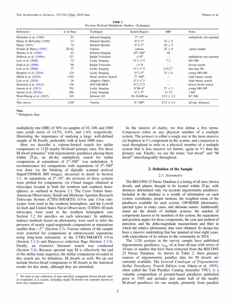
trigonometric parallaxes, πtrig, of at least 40 mas with errors of10 mas or smaller that have been extracted from the RECONS25 Parsec Database. As shown in Table 2, three primarysources of trigonometric parallax data for M dwarfs arecurrently available. The General Catalogue of TrigonometricStellar Parallaxes, Fourth Edition (van Altena et al. 1995),often called the Yale Parallax Catalog (hereafter YPC), is avaluable compendium of ground-based parallaxes publishedprior to 1995 and includes just under half of the nearbyM-dwarf parallaxes for our sample, primarily from parallax

Table 1

Previous M-dwarf Multiplicity Studies—Techniques

References # of Stars Technique Search Region MRa Notes

Skrutskie et al. (1989) 55 Infrared Imaging 2″–14″ L multiplicity not reportedHenry & McCarthy (1990) 27 Infrared Speckle 0 2–5″ 34±9Henry (1991) 74 Infrared Speckle 0 2–5″ 20±5Fischer & Marcy (1992) 28–62 Various various 42±9 varied sampleSimons et al. (1996) 63 Infrared Imaging 10″–240″ 40Delfosse et al. (1999a) 127 Radial Velocities <1.0″ L multiplicity not reportedLaw et al. (2006) 32 Lucky Imaging 0 1–1 5 7 3

7

-+ M5–M8

Endl et al. (2006) 90 Radial Velocities <1 0 L Jovian searchLaw et al. (2008) 77 Lucky Imaging 0 1–1 5 13.6 4

6.5

-+ late-type Ms

Bergfors et al. (2010) 124 Lucky Imaging 0 2–5″ 32±6 young M0–M6Dhital et al. (2010) 1342 Sloan Archive Search 7″–180″ L wide binary searchLaw et al. (2010) 36 Adaptive Optics 0 1–1 5 L wide binary searchDieterich et al. (2012) 126 HST-NICMOS 0 2–7 5 L brown dwarf searchJanson et al. (2012) 701 Lucky Imaging 0 08–6″ 27±3 young M0–M5Janson et al. (2014a) 286 Lucky Imaging 0 1–5″ 21–27 >M5Ward-Duong et al. (2015) 245 Infrared AO 10–10,000 au 23.5±3.2 K7–M6

This survey 1120 Various 0″–300″ 27.5±1.4 all trig. distances

Note.a Multiplicity Rate.

9 We refer to any collection of stars and their companion brown dwarfs and/or exoplanets as a system, including single M dwarfs not currently known tohave any companions.

2

The Astronomical Journal, 157:216 (32pp), 2019 June Winters et al.

programs at the Allegheny, Mt.Stromlo, McCormick, Sproul,US Naval, Van Vleck, Yale, and Yerkes Observatories. TheHipparcos mission (initial release by Perryman et al. (1997)and revised results used here by van Leeuwen (2007); hereafterHIP) updated 231 of those parallaxes, and contributed 229 newsystems for bright (V12.5) nearby M dwarfs. Overall, 743systems have parallaxes from the YPC and HIP catalogs.

The next largest collection of parallaxes measured for nearbyM dwarfs is from the RECONS10 team, contributing 308 reddwarf systems to the 25 pc census via new measurements(Costa et al. 2005, 2006; Jao et al. 2005, 2011, 2014, 2017;Henry et al. 2006, 2018; Subasavage et al. 2009; Riedel et al.2010, 2011, 2014, 2018; von Braun et al. 2011; Mamajeket al. 2013; Dieterich et al. 2014; Bartlett et al. 2017; Winterset al. 2017), published in The Solar Neighborhood series ofpapers (hereafter TSN) in The Astronomical Journal.11 Finally,other groups have contributed parallaxes for an additional 69nearby M dwarfs. As shown in Table 2, RECONS’ work in thesouthern hemisphere creates a balanced all-sky sample of Mdwarfs with known distances for the first time, as the southernhemisphere has historically been under-sampled. An importantaspect of the sample surveyed here is that because all 1120systems have accurate parallaxes, biases inherent to photo-metrically-selected samples are ameliorated.

A combination of color and absolute magnitude limits wasused to select a sample of bona fide M dwarfs. Stars within25 pc were evaluated to define the meaning of “M dwarf” byplotting spectral types from Reid et al. (1995), Hawley et al.(1996), Gray et al. (2003), and RECONS (Riedel et al. 2014)versus (V− K ) and MV. Because spectral types can beimprecise, there was overlap between the K and M types, soboundaries were chosen to split the types at carefully defined(V− K ) and MV values. A similar method was followed for theM-L dwarf transition using results primarily from Dahn et al.(2002). These procedures resulted in ranges of 8.8�MV�20.0 and 3.7�(V− K )�9.5 for stars we consider to beM dwarfs. For faint stars with no reliable V available, an initialconstraint of (I− K )�4.5 was used to create the sample untilV could be measured. These observational parameters corre-spond to masses of 0.63<M/Me<0.075, based on themass–luminosity relation (MLR) presented in Benedict et al.(2016). We note that no M dwarfs known to be companions tomore massive stars are included in this sample. Systems thatcontained a white dwarf component were excluded from thesample, as the white dwarf was previously the brighter andmore massive primary.

Imposing these distance, absolute magnitude, and colorcriteria yields a sample of 1120 red dwarf primaries as of 2014January 1, when the companion search sample list was frozen,with some new parallaxes measured by RECONS being addedas they became available. The astrometry data for these 1120systems are listed in Table 3. Included are the names of theM-dwarf primary, coordinates (J2000.0), proper motionmagnitudes and position angles with references, the weightedmeans of the published trigonometric parallaxes and the errors,and the number of parallaxes included in the weighted meanand references. We note that for multiple systems, the propermotion of the primary component has been assumed to be thesame for all members of the system. All proper motions arefrom SuperCOSMOS, except where noted. Proper motionswith the reference “RECONS (in prep)” indicate Super-COSMOS proper motions that will be published in theforthcoming RECONS 25 Parsec Database (W. C. Jao et al.2019, in preparation), as these values have not been presentedpreviously. In the cases of multiple systems for which parallaxmeasurements exist for companions as well as for theprimaries, these measurements have been combined in theweighted means. The five parallaxes noted as “in prep” will bepresented in upcoming papers in the TSN series. Figure 1shows the distribution on the sky of the entire sampleinvestigated for multiplicity. Note the balance in the distribu-tion of stars surveyed, with nearly equal numbers of M dwarfsin the northern and southern skies.

2.2. Sample Selection Biases

We describe here how the sample selection process couldbias the result of our survey.We note that our sample is volume-limited, not volume-

complete. If we assume that the 188 M-dwarf systems in oursample that lie within 10 pc comprise a volume-completesample and extrapolate to 25 pc assuming a uniform stellardensity, we expect 2938 M-dwarf systems to lie within 25 pc.We cross-matched our sample of M-dwarf primaries to the

recently available parallaxes from the Gaia Data Release 2(DR2; Gaia Collaboration et al. 2016, 2018) and found that90% (1008 primaries) had Gaia parallaxes that placed themwithin 25 pc. Four percent fell outside of 25 pc with a GaiaDR2 parallax. The remaining 6% (69 primaries) were not foundto have a Gaia DR2 parallax, but 47 (4%) are known to be inmultiple systems with separations between the components onthe order of or smaller than 1″. Nine of these 47 multiplesystems are within the 10 pc horizon. A few of the remaining22 that are not currently known to be multiple are definitivelynearby, but have high proper motion (e.g., GJ 406) or are bright(e.g., GJ 411). We do not make any corrections to our samplebased on this comparison because it is evident that a sample ofstars surveyed for stellar multiplicity based on the Gaia DR2would neglect binaries. We look forward, however, to the GaiaDR3, which will include valuable multiplicity information.Figure 2 shows the distribution of the apparent I magnitudes

of the red dwarfs surveyed, with a peak at I=8.5–9.5.Because brighter objects are generally targeted for parallaxmeasurements before fainter objects, for which measurementsare more difficult, 85% of the sample is made up of bright stars(I<12.00), introducing an implicit Malmquist bias. Asunresolved multiple systems are usually overluminous, thissurvey’s outcomes are biased toward a larger MR.

Table 2

Parallax Sources for Multiplicity Search

Reference # of Targets # of TargetsNorth of δ=0 South of δ=0

YPC 389 125HIP 83 146RECONS—published 31 272RECONS—unpublished 2 3Literature (1995–2012) 51 18

TOTAL 556 564

10 REsearch Consortium On Nearby Stars,www.recons.org.11 A few unpublished measurements used in this study are scheduled for aforthcoming publication in this series.

3


We have also required the error on the published trigono-metric parallax to be �10 mas in order to limit the sample tomembers that are reliably within 25 pc. Therefore it is possiblethat binaries were missed, as perturbations on the parallax dueto an unseen companion can increase the parallax error. Forty-five M-dwarf systems with YPC or HIP parallaxes wereeliminated from the sample due to their large parallax errors.

We cross-checked these 45 targets against the Gaia DR2 with asearch radius of 3′ to mitigate the positional offset of thesetypically high proper motion stars. Twenty-nine were returnedwith parallaxes by Gaia, 19 of which remained within ourchosen 25 pc distance horizon. Four of these 19 had closecompanions detected by Gaia. If we assumed that the 16 non-detections were all multiple systems and all within 25 pc, thesample size would increase to 1155, and the MR wouldincrease by 0.9%. We do not include any correction due to thisbias. We note that the parallaxes measured as a result ofRECONS’ astrometry program, roughly one-third of thesample, would not factor into this negative bias, as all of thesedata were examined and stars with astrometric perturbationsdue to unseen companions flagged.

Table 3

Astrometry Data

Name R.A. Decl. μ P.A. References π σπ # π References(hh:mm:ss) (dd:mm:ss) (″ yr−1

) (deg) (mas) (mas)(1) (2) (3) (4) (5) (6) (7) (8) (9) (10)

GJ1001ABC 00 04 36.45 −40 44 02.7 1.636 159.7 71 77.90 2.04 2 15, 68GJ1 00 05 24.43 −37 21 26.7 6.106 112.5 28 230.32 0.90 2 68, 69LHS1019 00 06 19.19 −65 50 25.9 0.564 158.7 72 59.85 2.64 1 69GJ1002 00 06 43.19 −07 32 17.0 2.041 204.0 39 213.00 3.60 1 68GJ1003 00 07 26.71 +29 14 32.7 1.890 127.0 38 53.50 2.50 1 68LHS1022 00 07 59.11 +08 00 19.4 0.546 222.0 38 44.00 6.30 1 68L 217−28 00 08 17.37 −57 05 52.9 0.370 264.0 40 75.17 2.11 1 73HIP687 00 08 27.29 +17 25 27.3 0.110 233.8 28 45.98 1.93 1 69G 131−26AB 00 08 53.92 +20 50 25.4 0.251 194.4 53 54.13 1.35 1 53GJ7 00 09 04.34 −27 07 19.5 0.715 079.7 72 43.61 2.56 2 68, 69LEHPM1−255 00 09 45.06 −42 01 39.6 0.271 096.7 72 53.26 1.51 1 73

Note.a The weighted mean parallax includes the parallax of both the primary and the secondary components.References.(1) Andrei et al. (2011); (2) Anglada-Escudé et al. (2012); (3) Bartlett et al. (2017); (4) Benedict et al. (1999); (5) Benedict et al. (2000); (6) Benedict et al.(2001); (7) Benedict et al. (2002); (8) Biller & Close (2007); (9) Costa et al. (2005); (10) Costa et al. (2006); (11) Dahn et al. (2002); (12) Deacon & Hambly (2001);(13) Deacon et al. (2005b); (14) Deacon et al. (2005a); (15) Dieterich et al. (2014); (16) Dupuy & Liu (2012); (17) Fabricius & Makarov (2000); (18) Faherty et al.(2012); (19) Falin & Mignard (1999); (20) Gatewood et al. (1993); (21) Gatewood et al. (2003); (22) Gatewood (2008); (23) Gatewood & Coban (2009); (24) Henryet al. (1997); (25) Henry et al. (2006); (26) Henry et al. (2018); (27) Hershey & Taff (1998); (28) Høg et al. (2000); (29) Ianna et al. (1996); (30) Jao et al. (2005); (31)Jao et al. (2011); (32) Jao et al. (2017); (33) Khovritchev et al. (2013); (34) Lèpine & Shara (2005); (35) Lèpine et al. (2009); (36) Lurie et al. (2014); (37) Luyten(1979a); (38) Luyten (1979b); (39) Luyten (1980a); (40) Luyten (1980b); (41) Martin & Mignard (1998); (42) Martinache et al. (2007); (43) Martinache et al. (2009);(44) Monet et al. (2003); (45) Pokorny et al. (2004); (46) Pourbaix et al. (2003); (47) Pravdo et al. (2006); (48) Pravdo & Shaklan (2009); (49) RECONS (in prep);(50) Reid et al. (2003); (51) Riedel et al. (2010); (52) Riedel et al. (2011); (53) Riedel et al. (2014); (54) Riedel et al. (2018); (55) Schilbach et al. (2009); (56) Schmidtet al. (2007); (57) Shakht (1997); (58) Shkolnik et al. (2012); (59) Smart et al. (2007); (60) Smart et al. (2010); (61) Söderhjelm (1999); (62) Subasavage et al. (2005a);(63) Subasavage et al. (2005b); (64) Teegarden et al. (2003); (65) Teixeira et al. (2009); (66) Tinney et al. (1995); (67) Tinney (1996); (68) van Altena et al. (1995);(69) van Leeuwen (2007); (70) von Braun et al. (2011); (71) Weis (1999); (72) Winters et al. (2015); (73) Winters et al. (2017).

(This table is available in its entirety in machine-readable form.)

Figure 1. Distribution on the sky of all 1120 M-dwarf primaries examined formultiplicity. Different colors indicate the different telescopes that were used forthe CCD imaging search: royal blue for the CTIO/SMARTS 0.9 m, dark greenfor the Lowell 42-inch, cyan for the CTIO/SMARTS 1.0 m, and bright greenfor the USNO 40-inch telescopes. The Galactic plane is outlined in gray.Illustrated is the uniformity of the sample in both hemispheres, due in large partto RECONS’ parallax work in the southern hemisphere.

Figure 2. Distribution of I-band magnitudes of our sample of 1120 M dwarfsknown to lie within 25 pc, illustrating that most (85%) of the target stars arebrighter than I=12.

4


Additionally, there is mass missing within 25 pc in the formof M-dwarf primaries (Winters et al. 2015). However, becausethe MRs decrease as a function of primary mass (seeSection 6.1.3 and Figure 19), the percentages of “missing”multiple systems in each mass bin are effectively equal. Basedon the 10 pc sample, as above, we expect 969 M dwarfs moremassive than 0.30 Me within 25 pc, but have 506 in oursample. The MR of 28.2% for the estimated 463 missingsystems results in 131 (14%) missing multiples in this primarymass subset. We expect 1109 M dwarfs with primaries0.15–0.30 Me within 25 pc, but have 402 in our sample. TheMR of 21.4% for the estimated 707 missing systems results in151 (14%) missing multiples in this primary mass subset.Finally, we expect 859 M dwarfs with primaries 0.075–0.15Me within 25 pc, but have 212 in our sample. The MR of16.0% for the estimated 647 missing systems results in 104(12%) missing multiples in this primary mass subset. Thereforewe do not include a correction for this bias.

2.3. Optical and Infrared Photometry

Existing VRI photometry for many of the M dwarfs in thesample was culled from the literature, much of which has beenpresented previously for the southern M dwarfs in Winterset al. (2011, 2015, 2017); however, a number of M dwarfs inthe sample had no published reliable optical photometryavailable. As part of the effort to characterize the M dwarfsin the survey, new absolute photometry in the Johnson–Kron–Cousins VJRKCIKC

12filters was acquired for 81, 3, and 49 stars

at the CTIO/SMARTS 0.9 m, CTIO/SMARTS 1.0 m, andLowell 42-inch telescopes, respectively, and is presented herefor the first time. Identical observational methods were used atall three sites. As in previous RECONS efforts, standard starfields from Graham (1982), Bessel (1990), and/or Landolt(1992, 2007, 2013) were observed multiple times each night toderive transformation equations and extinction curves. In orderto match those used by Landolt, apertures 14″in diameter wereused to determine the stellar fluxes, except in cases where closecontaminating sources needed to be deblended. In these cases,smaller apertures were used and aperture corrections wereapplied. Further details about the data reduction procedures,transformation equations, etc., can be found in Jao et al. (2005),Winters et al. (2011), and Winters et al. (2015).

In addition to the 0.9 m, 1.0 m, and 42-inch observations,three stars were observed at the USNO Flagstaff Station 40-inch telescope. Basic calibration frames, bias and sky flats ineach filter are taken either every night (bias) or over multiplenights in a run (sky flats) and are applied to the raw sciencedata. Standard star fields from Landolt (2009, 2013) wereobserved at multiple airmasses between ∼1.0 and ∼2.1 eachper night to calculate extinction curves. All instrumentalmagnitudes, both for standards and science targets, areextracted by fitting spatially-dependent point-spread functions(PSFs) for each frame using Source Extractor (SExtractor;Bertin & Arnouts 1996) and PSFEx (Bertin 2011), with anaperture diameter of 14″. Extensive comparisons of thistechnique to basic aperture photometry have producedconsistent results in uncrowded fields.

Optical and infrared photometry for the 1448 components ofthe 1120 M-dwarf systems is presented in Table 4, whereavailable. JHKs magnitudes were extracted from 2MASS(Skrutskie et al. 2006) and confirmed by eye to correspond tothe star in question during the blinking survey. Included are thenames of the M dwarfs (Column 1), the number of knowncomponents in the systems (2), J2000.0 coordinates (3, 4), VRImagnitudes (5, 6, 7), the number of observations and/orreferences (8), the 2MASS JHKs magnitudes (9, 10, 11), andthe photometric distance estimate. Next are listed the ΔVmagnitudes between stellar companions and primaries (12), thedeblended V magnitudes Vdb (13), and estimated masses foreach component (14). Components of multiple systems arenoted with a capital letter (A, B, C, D, E) after the name in thefirst column. If the names of the components are different, theletters identifying the primary and the secondary are placedwithin parentheses, e.g., LHS1104(A) and LHS1105(B). If thestar is a companion in a multiple system, “0” is given inColumn (2). “J” for joint photometry is listed with eachblended magnitude. Brown dwarf companions are noted by a“BD” next to the “0” in Column 2, and often do not havecomplete photometry, if any.For new photometry reported here, superscripts are added to

the references indicating which telescope(s) was used toacquire the VRI photometry: “09” for the CTIO/SMARTS0.9 m, “10” for the CTIO/SMARTS 1.0 m, “40” for the USNO40-inch telescope, and “42” for the Lowell 42-inch telescope. Ifthe ΔV is larger than 3, the magnitude of the primary is treatedas unaffected by the companion(s). All masses are estimatedfrom the absolute V magnitude, which has been calculated fromthe deblended V magnitude for each star in Column (13), theparallax in Table 3, and the empirical MLRs of Benedict et al.(2016). If any type of assumption or conversion was maderegarding the ΔV (as discussed in Section 5.3.1), it is noted.As outlined in Winters et al. (2011), photometric errors at the

0.9 m are typically 0.03 mag in V and 0.02 mag in R and I. Toverify the Lowell 42-inch data,13 Table 5 presents photometryfor four stars observed at the Lowell 42-inch and at the CTIO/SMARTS 0.9 m telescopes, as well as six stars with VRI fromthe literature. Results from the 42-inch and 0.9 m telescopesmatch to 0.06 mag, except for the R magnitude of GJ 1167,which can be attributed to a possible flare event observed at thetime of observation at the 42-inch telescope, as the V and Imagnitudes are consistent. This object is, in fact, included in aflare star catalog of UV Cet-type variables (Gershberg et al.1999). An additional six stars were observed by Weis,14 andthe photometry matches to within 0.08 mag for all six objects,and typically to 0.03 mag. Given our typical 1σ errors of atmost 0.03 mag for VRI, we find that the Lowell 42-inch datahave differences of 2σ or smaller in 28 of the 30 cases shown inTable 5.

3. The Searches and Detected Companions

Several searches were carried out on the 1120 nearby Mdwarfs in an effort to make this the most comprehensiveinvestigation of multiplicity ever undertaken for stars thatdominate the solar neighborhood. Information about the

12 These subscripts will be dropped henceforth. The central wavelengths forthe VJ, RKC, and IKC filters at the 0.9 m are 5438 Å, 6425 Å, and 8075 Å,respectively; filters at other telescopes are similar.

13 No rigorous comparisons are yet possible for our sample of red dwarfs forthe CTIO/SMARTS 1.0 m and USNO 40-inch telescopes because only threestars have been observed at each.14 All photometry from Weis has been converted to the Johnson–Kron–Cousins (JKC) system using the relation in Bessell & Weis (1987).

5


Table 4

Photometry Data

Name # Obj R.A. Decl. VJ RKC IKC # nts/ref J H Ks πccd σπ ΔV Vdb Mass(dd:mm:ss) (hh:mm:ss) (mag) (mag) (mag) (mag) (mag) (mag) (pc) (pc) (mag) (mag) (Me)

(1) (2) (3) (4) (5) (6) (7) (8) (9) (10) (11) (12) (13) (14) (15) (16)

GJ 1001B 0BD 00 04 34.87 −40 44 06.5 22.77J 19.04J 16.67J /10d 13.11J 12.06J 11.40J L L L L L

GJ 1001C 0BD 00 04 34.87 −40 44 06.5 L L L L L L L L L L L L

GJ 1001A 3 00 04 36.45 −40 44 02.7 12.83 11.62 10.08 /40 8.60 8.04 7.74 12.5 1.9 L 12.83 0.234GJ 1 1 00 05 24.43 −37 21 26.7 8.54 7.57 6.41 /4 5.33 4.83a 4.52 5.6 0.9 L 8.54 0.411LHS 1019 1 00 06 19.19 −65 50 25.9 12.17 11.11 9.78 /21 8.48 7.84 7.63 16.6 2.6 L 12.17 0.335GJ 1002 1 00 06 43.19 −07 32 17.0 13.84 12.21 10.21 /40 8.32 7.79 7.44 5.4 1.0 L 13.84 0.116GJ 1003 1 00 07 26.71 +29 14 32.7 14.16 13.01 11.54 /37 10.22 9.74 9.46 36.0 7.0 L 14.16 0.203LHS 1022 1 00 07 59.11 +08 00 19.4 13.09 12.02 10.65 /37 9.39 8.91 8.65 28.9 5.2 L 13.09 0.311L 217-28 1 00 08 17.37 −57 05 52.9 12.13 11.00 9.57 /40 8.21 7.63 7.40 13.2 2.0 L 12.13 0.293HIP 687 1 00 08 27.29 +17 25 27.3 10.80 9.88 8.93 /35 7.81 7.17 6.98 18.5 3.2 L 10.80 0.582

Notes. A “J” next to a photometry value indicates that the magnitude is blended due to one or more close companions. A square bracket next to the photometric distance estimate indicates that the joint photometry of themultiple system was used to calculate the distance estimate, which is thus likely underestimated. A “u” following the photometry reference indicates that we present an update to previously presented RECONSphotometry.a 2MASS magnitude error greater than 0.05 mag.b An assumption was made regarding the Δmag.c A conversion to ΔV was done from a reported magnitude difference in another filter.d Photometry in SOAR filters and not converted to Johnson–Kron–Cousins system.e Mass from Barbieri et al. (1996).f Mass from Benedict et al. (2000).g Mass from Benedict et al. (2016).h Mass from Henry et al. (1999).i Mass from Henry et al. (1999), Tamazian et al. (2006).j Mass from Ségransan et al. (2000).k Mass from Delfosse et al. (1999a).l Mass from Díaz et al. (2007).m Mass from Duquennoy & Mayor (1988).n Mass from Herbig & Moorhead (1965).o Photometry for “AC” instead of for the “B” component was mistakenly reported in Davison et al. (2015).References.(1) This work; (2) Bartlett et al. (2017); (3) Benedict et al. (2016); (4) Bessel (1990); (5) Bessell (1991); (6) Costa et al. (2005); (7) Costa et al. (2006); (8) Dahn et al. (2002); (9) Davison et al. (2015);(10) Dieterich et al. (2014); (11) Harrington & Dahn (1980); (12) Harrington et al. (1993); (13) Henry et al. (2006); (14) Henry et al. (2018); (15) Høg et al. (2000); (16) Hosey et al. (2015); (17) Jao et al. (2005); (18) Jaoet al. (2011); (19) Jao et al. (2017); (20) Koen et al. (2002); (21) Koen et al. (2010); (22) Lèpine et al. (2009); (23) Lurie et al. (2014); (24) Reid et al. (2002); (25) Riedel et al. (2010); (26) Riedel et al. (2011); (27) Riedelet al. (2014); (28) Riedel et al. (2018); (29) Weis (1984); (30) Weis (1986); (31) Weis (1987); (32) Weis (1988); (33) Weis (1991b); (34) Weis (1991a); (35) Weis (1993); (36) Weis (1994); (37) Weis (1996); (38) Weis(1999); (39) Winters et al. (2011); (40) Winters et al. (2015); (41) Winters et al. (2017).


6

TheAstronomicalJournal,157:216

(32pp),2019

JuneWinters

etal.

surveys is collected in Tables 6–12, including a statisticaloverview of the individual surveys in Table 6. Note that thenumber of detections includes confirmations of previouslyreported multiples in the literature. Specifics about the BlinkSurvey are listed in Table 7. Telescopes used for the CCDImaging Survey in Table 8, while detection limit informationfor the CCD Imaging Survey is presented in Tables 9 and 10.Results for confirmed multiples are collected in Table 11,whereas candidate (as yet unconfirmed) companions are listedin Table 12.

We report the results of each search here; overall results arepresented in Section 5.

3.1. Wide-field Blinking Survey: Companions at 5″–300″

Because most nearby stars have large proper motions,images of the stars taken at different epochs were blinked forcommon proper motion (CPM) companions with separations of5″–300″. A wide companion would have a similar propermotion to its primary and would thus appear to move in thesame direction at the same speed across the sky. ArchivalSuperCOMOS B R IJ F IVN59

15 photographic plate images10′×10′in size were blinked using the Aladin interface ofthe Centre de Données astronomiques de Strasbourg (CDS) todetect companions at separations greater than ∼5″. Theseplates were taken from 1974 to 2002 and provide up to 28 yearsof temporal coverage, with typical epoch spreads of at least 10years. Information for the images blinked is given in Table 7,taken from Morgan (1995), Subasavage (2007), and the UKSchmidt webpage.16 Candidates were confirmed to be real bycollecting VRI photometry and estimating photometric

distances using the suite of relations in Henry et al. (2004); ifthe distances of the primary and candidate matched to withinthe errors on the distances, the candidate was deemed to be aphysical companion. In addition to recovering 63 known CPMcompanions, one new CPM companion (2MA0936−2610C)was discovered during this blinking search, details of which aregiven in Section 4.1. No comprehensive search for companionsat angular separations larger than 300″was conducted.

3.1.1. Blink Survey Detection Limits

The CPM search had two elements that needed to beevaluated in order to confidently identify objects moving withthe primary star in question: companion brightness and the sizeof each system’s proper motion.A companion would have to be detectable on at least two of

the three photographic plates in order to notice its propermotion, so any companion would need to be brighter than themagnitude limits given in Table 7 in at least two images.Because the search is for stellar companions, it is onlynecessary to be able to detect a companion as faint as thefaintest star in the sample, effectively spectral type M9.5 V at25 pc. The two faintest stars in the sample are DEN 0909−0658, with VRI=21.55, 19.46, and 17.18 and RG0050−2722 with VRI=21.54, 19.09, and 16.65. The B magnitudes

Table 5

Overlapping Photometry Data

Name (V − K ) VJ RKC IKC # obs tel/ref(mag) (mag) (mag) (mag)

2MAJ0738+2400

4.86 12.98 11.81 10.35 1 42in

12.98 11.83 10.35 2 0.9 mG 43−2 4.76 13.23 12.08 10.67 1 42in

13.24 12.07 10.66 2 0.9 m2MAJ1113

+10255.34 14.55 13.27 11.63 1 42in

14.50 13.21 11.59 2 0.9 mGJ1167 5.59 14.16 12.67 11.10 1 42in

14.20 12.82 11.11 1 0.9 m

LTT17095A 4.22 11.12 10.12 9.00 1 42in11.11 10.11 8.94 L 1

GJ15B 5.12 11.07 9.82 8.34 2 42in11.06 9.83 8.26 L 3

GJ507AC 3.96 9.52 8.56 7.55 1 42in9.52 8.58 7.55 L 3

GJ507B 4.64 12.15 11.06 9.66 1 42in12.12 11.03 9.65 L 3

GJ617A 3.64 8.59 7.68 6.85 1 42in8.60 7.72 6.86 L 3

GJ617B 4.67 10.74 9.67 8.29 1 42in10.71 9.63 8.25 L 2

References.(1) Weis (1993); (2) Weis (1994); (3) Weis (1996).

Table 6

Companion Search Technique Statistics

Technique Separation Searched Searched Detected(″) (#) (%) (#)

Image Blinking 5–300 1110 99 64CCD Imaging 2–10 1120 100 44RECONS Perturbations <2 324 29 39HR Diagram Elevation <2 1120 100 11Distance Mismatches <2 1112 99 37Hipparcos Flags <2 460 41 31Literature/WDS Search all 1120 100 290Individual companions TOTAL 1120 100 310

Table 7

Blink Survey Information

Filter Epoch Span Decl. RangeMag.Limit Δλ

(yr) (deg) (mag) (Å)

BJ (IIIaJ) 1974–1994 all-sky ∼20.5 3950–5400R59F (IIIaF) 1984–2001 all-sky ∼21.5 5900–6900IIVN (IVN) 1978–2002 all-sky ∼19.5 6700–9000EPOSS–I

(103aE)1950–1957 −20.5<δ<+05 ∼19.5 6200–6700

IKC 2010–2014 all sky ∼17.5 7150–9000

Table 8

Telescopes Used for CCD Imaging Search and VRI Photometry

Telescope FOV Pixel Scale # Nights # Objects

Lowell 42in 22 3×22 3 0 327 px−1 21 508USNO 40in 22 9×22 9 0 670 px−1 1 22CTIO/SMARTS 0.9 m

13 6×13 6 0 401 px−1 16 442

CTIO/SMARTS 1.0 m

19 6×19 6 0 289 px−1 8 148

15 These subscripts will be dropped henceforth.16 http://www.roe.ac.uk/ifa/wfau/ukstu/telescope.html

7


for these stars are both fainter than the mag∼20.5 limit of theB plate, and thus neither star was detected in the B image;however, their R and I magnitudes are both brighter than thelimits of those plates and the stars were identified in both the Rand I images. Ten other objects are too faint to be seen on the Bplate, but as is the case with DEN0909−0658 and RG0050−2722, all are bright enough for detection in the R and Iimages.

The epoch spread between the plates also needed to be largeenough to detect the primary star moving in order to then noticea companion moving in tandem with it. As shown in thehistogram of proper motions in Figure 3, most of the surveystars move faster than 0 18 yr−1, the historical cutoff ofLuyten’s proper motion surveys. Hence, even a 10 yr baselineprovides 1 8 of motion, our adopted minimum proper motiondetection limit, easily discerned when blinking plates. How-ever, 58 of the stars in the survey (∼5% of the sample) haveμ < 0 18 yr−1, with the slowest star having μ= 0 03 yr−1; forthis star, to detect a motion of 1 8, the epoch spread wouldneed to be 60 yr. For 18 stars with decl. −20 < δ < +5°, theolder POSS-I plate (taken during 1950–1957) was used for theslow-moving primaries. This extended the epoch spread by8–24 yr, enabling companions for these 18 stars to be detected,leaving 40 slow-moving stars to search.

The proper motions of 151 additional primaries were notinitially able to be detected confidently because the epochspread of the SuperCOSMOS plates was shorter than 5 yr.These 151 stars, in addition to the 40 stars with low μmentioned above that were not able to be blinked using the

POSS plates, were compared to our newly acquired I-bandimages taken during the CCD Imaging Survey, extending theepoch spread by almost 20 years in some cases. Whereverpossible, the SuperCOSMOS I-band image was blinked withour CCD I-band image, but sometimes a larger epoch spreadwas possible with either the B- or R-band plate images. In thesecases, the plate that provided the largest epoch spread wasused. In order to upload these images to Aladin to blink withthe archival SuperCOSMOS images, World Coordinate System(WCS) coordinates were added to the header of each image sothat the two images could be aligned properly. This was doneusing SExtractor for the CTIO/SMARTS 0.9 m and the USNO40-inch images and the tools at Astrometry.net for the Lowell42-inch and the CTIO/SMARTS 1.0 m images.After using the various techniques outlined above to extend

the image epoch spreads, 1110 of 1120 stars were sucessfullysearched in the Blink Survey for companions. In 10 cases,either the primary star’s proper motion was still undetectable,the available CCD images were taken under poor skyconditions and many faint sources were not visible, or theframe rotations converged poorly. A primary result from thisBlink Survey is that in the separation regime from 10″ to 300″,where the search is effectively complete, we find an MR of4.7% (as discussed in Section 5.2). Thus, we estimate that only0.5 CPM stellar companions (10∗4.7%) with separations 10″–300″ were missed due to not searching 10 stars during theBlinking Survey.

Table 9

Stars Used for Imaging Search Detection Limit Study

Name I FWHM Tel Note(mag) (arcsec)

GJ285 8.24 0.8 0.9 mLP848−50AB 12.47J 0.8 0.9 m ρAB<2″SIP1632−0631 15.56 0.8 0.9 mL 32−9A 8.04 1.0 0.9 m ρAB=22 40SCR0754−3809 11.98 1.0 0.9 mBRI1222−1221 15.59 1.0 0.9 mGJ709 8.41 1.0 42inGJ1231 12.08 1.0 42inReference Star 16 (scaled) 1.0 42inGJ2060AB 7.83J 1.5 0.9 m ρAB=0 4852MA2053−0133 12.46 1.5 0.9 mReference Star 16 (scaled) 1.5 0.9 mGJ109 8.10 1.5 42inLHS1378 12.09 1.5 42in2MA0352+0210 16.12 1.5 42inReference Star 8 (scaled) 1.8 0.9 mSCR2307−8452 12.00 1.8 0.9 mReference Star 16 (scaled) 1.8 0.9 mGJ134 8.21 1.8 42inLHS1375 12.01 1.8 42inSIP0320−0446AB 16.37 1.8 42in ρAB<0 33GJ720A 8.02 2.0 42in ρAB=112 10LHS3005 11.99 2.0 42in2MA1731+2721 15.50 2.0 42in

Note.“J” on the I-band magnitudes of LP848−50AB and GJ2060ABindicates that the photometry includes light from the companion. The othersubarcsecond binary, SIP0320−0446AB, has a brown dwarf companion thatdoes not contribute significant light to the photometry of its primary star.

Table 10

Imaging Search Detection Limit Summary

Seeing Yes No Maybe Yes No MaybeConditions (#) (#) (#) (#) (#) (#)

0.9 m 42in

FWHM=0 8 64 8 3 L L L

I=8 mag 36 7 2 L L L

I=12 mag 23 1 1 L L L

I=16 mag 5 L L L L L

FWHM=1 0 62 8 5 60 12 3

I=8 mag 35 7 3 34 8 3I=12 mag 22 1 2 21 4 L

I=16 mag 5 L L 5 L L

FWHM=1 5 58 12 5 55 12 8

I=8 mag 33 9 3 33 6 6I=12 mag 20 3 2 17 6 2I=16 mag 5 L L 5 L L

FWHM=1 8 50 18 7 52 14 9

I=8 mag 28 13 4 29 10 6I=12 mag 18 5 2 19 4 2I=16 mag 4 L 1 4 L 1

FWHM=2 0 L L L 46 17 12

I=8 mag L L L 24 12 9I=12 mag L L L 18 5 2I=16 mag L L L 4 L 1

TOTAL 234 46 20 213 55 32

8


3.2. CCD Imaging Survey: Companions at 2″–10″

To search for companions with separations 2″–10″, astro-metry data were obtained at four different telescopes: in thenorthern hemisphere, the Hall 42-inch telescope at LowellObservatory and the USNO 40-inch telescope, both inFlagstaff, AZ, and in the southern hemisphere, the CTIO/SMARTS 0.9 m and 1.0 m telescopes, both at Cerro TololoInter-American Observatory in Chile. Each M-dwarf primarywas observed in the IKC filter with integrations of 3, 30, and300 seconds in order to reveal stellar companions at separations2″–10″. This observational strategy was adopted to reveal anyclose equal-magnitude companions with the short 3 s expo-sures, while the long 300 s exposures would reveal faintcompanions with masses at the end of the main sequence. The30 s exposures were taken to bridge the intermediate phasespace. Calibration frames taken at the beginning of each nightwere used for typical bias subtraction and dome flat-fieldingusing standard IRAF procedures.

Technical details for the cameras and specifics about theobservational setups and numbers of nights and stars observedat each telescope are given in Table 8. The telescopes used for

the imaging campaign all have primary mirrors roughly 1 m insize and have CCD cameras that provide similar pixel scales.Data from all telescopes were acquired without binning pixels.The histogram in Figure 4 illustrates the seeing measured forthe best images of each star surveyed at the four differenttelescopes. Seeing conditions better than 2″ were attained forall but one star, GJ 507, with some stars being observedmultiple times. While the 0.9 m telescope has a slightly largerpixel scale than the 1.0 m and the 42-inch telescopes, as shownin Figure 4, the seeing was typically better at that site, allowingfor better resolution. Only 22 primaries (fewer than 2% of thesurvey) were observed at the USNO 40-inch telescope, so wedo not consider the coarser pixel scale to have significantlyaffected the survey. Overall, the data from the four telescopesused were of similar quality and the results could be combinedwithout modification.A few additional details of the observations are worthy

of note:

1. A total of 442 stars were observed at the CTIO/SMARTS0.9 m telescope, where consistently good seeing, tele-scope operation, and weather conditions make

Table 11

Multiplicity Information for Sample

Name # Obj Map R.A. Decl. ρ θ Year Technique References Δmag Filter References(hh:mm:ss) (dd:mm:ss) (″) (deg) (mag)

GJ1001 0 BC 00 04 34.87 −40 44 06.5 0.087 048 2003 HSTACS 40 0.01 222 40GJ1001 3 A-BC 00 04 36.45 −40 44 02.7 18.2 259 2003 visdet 40 9.91 VJ 1G 131−26 2 AB 00 08 53.92 +20 50 25.4 0.111 170 2001 AO det 13 0.46 H 13GJ11 2 AB 00 13 15.81 +69 19 37.2 0.859 089 2012 lkydet 62 0.69 i′ 62LTT17095 2 AB 00 13 38.74 +80 39 56.8 12.78 126 2001 visdet 103 3.63 VJ 1GJ1005 2 AB 00 15 28.06 −16 08 01.8 0.329 234 2002 HSTNIC 30 2.42 VJ 92MA0015−1636 2 AB 00 15 58.07 −16 36 57.8 0.105 090 2011 AO det 18 0.06 H 18L 290−72 2 AB 00 16 01.99 −48 15 39.3 <1 L 2007 SB1 117 L L ...GJ1006 2 AB 00 16 14.62 +19 51 37.6 25.09 059 1999 visdet 103 0.94 VJ 111GJ15 2 AB 00 18 22.88 +44 01 22.7 35.15 064 1999 visdet 103 2.97 VJ 1

Note. The codes for the techniques and instruments used to detect and resolve systems are: AO det—adaptive optics; astdet —detection via astrometric perturbation,companion often not detected directly; astorb—orbit from astrometric measurements; HSTACS—Hubble Space Telescope’s Advanced Camera for Surveys; HSTFGS—Hubble Space Telescope’s Fine Guidance Sensors; HSTNIC—Hubble Space Telescope’s Near Infrared Camera and Multi-Object Spectrometer; HSTWPC—Hubble Space Telescope’s Wide Field Planetary Camera 2; lkydet—detection via lucky imaging; lkyorb—orbit from lucky imaging measurements; radorb—orbitfrom radial velocity measurements; radvel— detection via radial velocity, but no SB type indicated; SB (1, 2, 3)—spectroscopic multiple, either single-lined, double-lined, or triple-lined; spkdet—detection via speckle interferometry; spkorb—orbit from speckle interferometry measurements; visdet—detection via visual astrometry;visorb—orbit from visual astrometry measurements.References.(1) This work; (2) Allen & Reid (2008); (3) Al-Shukri et al. (1996); (4) Balega et al. (2007); (5) Balega et al. (2013); (6) Bartlett et al. (2017); (7)Benedict et al. (2000); (8) Benedict et al. (2001); (9) Benedict et al. (2016); (10) Bergfors et al. (2010); (11) Bessel (1990); (12) Bessell (1991); (13) Beuzit et al.(2004); (14) Biller et al. (2006); (15) Blake et al. (2008); (16) Bonfils et al. (2013); (17) Bonnefoy et al. (2009); (18) Bowler et al. (2015); (19) Burningham et al.(2009); (20) Chanamé & Gould (2004); (21) Cortes-Contreras et al. (2014); (22) Cvetković et al. (2015); (23) Daemgen et al. (2007); (24) Dahn et al. (1988); (25)Davison et al. (2014); (26) Dawson & De Robertis (2005); (27) Delfosse et al. (1999a); (28) Delfosse et al. (1999b); (29) Díaz et al. (2007); (30) Dieterich et al.(2012); (31) Docobo et al. (2006); (32) Doyle & Butler (1990); (33) Duquennoy & Mayor (1988); (34) Femenía et al. (2011); (35) Forveille et al. (2005); (36) Freedet al. (2003); (37) Fu et al. (1997); (38) Gizis (1998); (39) Gizis et al. (2002); (40) Golimowski et al. (2004); (41) Harlow (1996); (42) Harrington et al. (1985); (43)Hartkopf et al. (2012); (44) Heintz (1985); (45) Heintz (1987); (46) Heintz (1990); (47) Heintz (1991); (48) Heintz (1992); (49) Heintz (1993); (50) Heintz (1994);(51) Henry et al. (1999); (52) Henry et al. (2006); (53) Henry et al. (2018); (54) Herbig & Moorhead (1965); (55) Horch et al. (2010); (56) Horch et al. (2011a); (57)Horch et al. (2012); (58) Horch et al. (2015a); (59) Ireland et al. (2008); (60) Janson et al. (2012); (61) Janson et al. (2014a); (62) Janson et al. (2014b); (63) Jao et al.(2003); (64) Jao et al. (2009); (65) Jao et al. (2011); (66) Jenkins et al. (2009); (67) Jódar et al. (2013); (68) Köhler et al. (2012); (69) Kürster et al. (2009); (70)Lampens et al. (2007); (71) Law et al. (2006); (72) Law et al. (2008); (73) Leinert et al. (1994); (74) Lèpine et al. (2009); (75) Lindegren et al. (1997); (76) Luyten(1979a); (77) Malo et al. (2014); (78) Martín et al. (2000); (79) Martinache et al. (2007); (80) Martinache et al. (2009); (81) Mason et al. (2009); (82) Mason et al.(2018); (83) McAlister et al. (1987); (84) Montagnier et al. (2006); (85) Nidever et al. (2002); (86) Pravdo et al. (2004); (87) Pravdo et al. (2006); (88) Reid et al.(2001); (89) Reid et al. (2002); (90) Reiners & Basri (2010); (91) Reiners et al. (2012); (92) Riddle et al. (1971); (93) Riedel et al. (2010);(94) Riedel et al. (2014);(95)Riedel et al. (2018); (96) Salim & Gould (2003); (97) Schneider et al. (2011); (98) Scholz (2010); (99) Ségransan et al. (2000); (100) Shkolnik et al. (2010); (101)Shkolnik et al. (2012); (102) Siegler et al. (2005); (103) Skrutskie et al. (2006); (104) Tokovinin & Lépine (2012); (105) van Biesbroeck (1974); (106) van Dessel &Sinachopoulos (1993); (107) Wahhaj et al. (2011); (108) Ward-Duong et al. (2015); (109) Weis (1991b); (110) Weis (1993); (111) Weis (1996); (112) Winters et al.(2011); (113) Winters et al. (2017); (114) Winters et al. (2018); (115) Woitas et al. (2003); (116) Worley & Mason (1998); (117) Zechmeister et al. (2009).


9


Table 12

Suspected Multiple Systems

Name # Stars R.A. Decl. Flag Reference(hh:mm:ss) (dd:mm:ss)

GJ 1006A 3? 00 16 14.62 +19 51 37.6 dist 1HIP 6365 2? 01 21 45.39 −46 42 51.8 X 3LHS 1288 2? 01 42 55.78 −42 12 12.5 X 3GJ 91 2? 02 13 53.62 −32 02 28.5 X 3G 143.3 2? 03 31 47.14 +14 19 17.9 X 3BD-21 1074A 4? 05 06 49.47 −21 35 03.8 dist 1GJ 192 2? 05 12 42.22 +19 39 56.5 X 3GJ 207.1 2? 05 33 44.81 +01 56 43.4 possSB 4SCR 0631-8811 2? 06 31 31.04 −88 11 36.6 elev 1LP 381-4 2? 06 36 18.25 −40 00 23.8 G 3SCR 0702-6102 2? 07 02 50.36 −61 02 47.7 elev,pb? 1,1LP 423-31 2? 07 52 23.93 +16 12 15.0 elev 1SCR 0757-7114 2? 07 57 32.55 −71 14 53.8 dist 1GJ 1105 2? 07 58 12.70 +41 18 13.4 X 3LHS 2029 2? 08 37 07.97 +15 07 45.6 X 3LHS 259 2? 09 00 52.08 +48 25 24.7 elev 1GJ 341 2? 09 21 37.61 −60 16 55.1 possSB 4GJ 367 2? 09 44 29.83 −45 46 35.6 X 3GJ 369 2? 09 51 09.63 −12 19 47.6 X 3GJ 373 2? 09 56 08.68 +62 47 18.5 possSB 4GJ 377 2? 10 01 10.74 −30 23 24.5 dist 1GJ 1136A 3? 10 41 51.83 −36 38 00.1 X,possSB 3,4GJ 402 2? 10 50 52.02 +06 48 29.4 X 3LHS 2520 2? 12 10 05.59 −15 04 16.9 dist 1GJ 465 2? 12 24 52.49 −18 14 32.3 pb? 2DEN 1250-2121 2? 12 50 52.65 −21 21 13.6 elev 1GJ 507.1 2? 13 19 40.13 +33 20 47.7 X 3GJ 540 2? 14 08 12.97 +80 35 50.1 X 32MA 1507-2000 2? 15 07 27.81 −20 00 43.3 dist,elev 1G 202-16 2? 15 49 36.28 +51 02 57.3 G 3LHS 3129A 3? 15 53 06.35 +34 45 13.9 dist 1GJ 620 2? 16 23 07.64 −24 42 35.2 G 3GJ 1203 2? 16 32 45.20 +12 36 45.9 X 3LP 69-457 2? 16 40 20.65 +67 36 04.9 elev 1LTT 14949 2? 16 40 48.90 +36 18 59.9 X 3HIP 83405 2? 17 02 49.58 −06 04 06.5 X 3LP 44-162 2? 17 57 15.40 +70 42 01.4 elev 1LP 334-11 2? 18 09 40.72 +31 52 12.8 X 3SCR 1826-6542 2? 18 26 46.83 −65 42 39.9 elev 1LP 44-334 2? 18 40 02.40 +72 40 54.1 elev 1GJ 723 2? 18 40 17.83 −10 27 55.3 X 3HIP 92451 2? 18 50 26.67 −62 03 03.8 possSB 4LHS 3445A 3? 19 14 39.15 +19 19 03.7 dist 1GJ 756 2? 19 21 51.42 +28 39 58.2 X 3LP 870-65 2? 20 04 30.79 −23 42 02.4 dist 1GJ 1250 2? 20 08 17.90 +33 18 12.9 dist 1LEHPM 2-783 2? 20 19 49.82 −58 16 43.0 elev 1GJ 791 2? 20 27 41.65 −27 44 51.9 X 3LHS 3564 2? 20 34 43.03 +03 20 51.1 X 3GJ 811.1 2? 20 56 46.59 −10 26 54.8 X 3L 117-123 2? 21 20 09.80 −67 39 05.6 X 3HIP 106803 2? 21 37 55.69 −63 42 43.0 X 3LHS 3748 2? 22 03 27.13 −50 38 38.4 X 3G 214-14 2? 22 11 16.96 +41 00 54.9 X 3GJ 899 2? 23 34 03.33 +00 10 45.9 X 3GJ 912 2? 23 55 39.77 −06 08 33.2 X 3

Note.Flag description: “dist” means that the ccddist is at least 2 times closer than the trigdist due to the object’s overluminousity; “elev” means that the object is elevatedabove the main sequence in the HR diagram in Figure 10 due to overluminosity; “possSB” means that the object has been noted as a possible spectroscopic binary by Reinerset al. (2012); “pb?” indicates that a possible perturbation was noted. The the single letters are Hipparcos reduction flags as follows: G is an acceleration solution where acomponent might be causing a variation in the proper motion; V is for variability-induced movers, where one component in an unresolved binary could be causing thephotocenter of the system to be perturbed; X is for a stochastic solution, where no reliable astrometric parameters could be determined, and which may indicate an astrometricbinary.References.(1) This work; (2) Heintz (1986); (3) Lindegren et al. (1997); (4) Reiners et al. (2012).

10


observations at this site superior to those at the othertelescopes used, as illustrated in Figure 4.

2. While being re-aluminized in 2012 December, the primarymirror at the Lowell 42-inch telescope was dropped anddamaged. The mask that was installed over the damagedmirror as a temporary fix resulted in a PSF flare before abetter mask was installed that slightly improved the PSF. Ofthe 508 stars observed for astrometry at Lowell, 457 wereobserved before the mishap and 51 after.

3. I-band images at both the Lowell 42-inch and CTIO/SMARTS 1.0 m telescopes suffer from fringing, themajor cause of which is night sky emission fromatmospheric OH molecules. This effect sometimes occurswith back-illuminated CCDs at optical wavelengthslonger than roughly 700 nm where the light is reflectedseveral times between the internal front and back surfacesof the CCD, creating constructive and destructiveinterference patterns, or fringing (Howell 2000, 2012).In order to remove these fringes, I-band frames frommultiple nights with a minimum of saturated stars in theframe were selected, boxcar smoothed, and then average-combined into a fringe map. This fringe map was thensubtracted from all I-band images using a modified IDLcode originally crafted by Snodgrass & Carry (2013).

Four new companions were discovered during this portion ofthe survey. Details on these new companions are given inSection 4.1. In each case, archival SuperCOSMOS plates wereblinked to eliminate the possibility that new companions werebackground objects. We detected 32 companions with separa-tions 2″–10″, as well as 12 companions with ρ<2″, includingthe four noted above.

3.2.1. CCD Imaging Survey Detection Limits

The MI range of the M-dwarf sequence is roughly 8magnitudes (MI=6.95–14.80 mag, specifically, for oursample). Therefore an analysis of the detection limits of theCCD imaging campaign was done for objects with a range of Imagnitudes at ρ=1″–5″ and at Δmags=0–8 in one-magnitude increments for different seeing conditions at thetwo main telescopes where the bulk (85%) of the stars wereimaged: the CTIO/SMARTS 0.9 m and the Lowell 42-inchtelescopes. While the companion search in the CCD framesextended to 10″, sources were detected even more easily atseparations 5″–10″ than at 5″, so it was not deemed necessaryto perform the analysis for the larger separations.Because the apparent I-band magnitudes for the stars in the

sample range from 5.32 to 17.18 (as shown in Figure 2),objects with I-band magnitudes of approximately 8, 12, and 16were selected for investigation. Only 88 primaries (7.8% of thesample) have I<8, so it was not felt necessary to create aseparate set of simulations for these brighter stars. The starsused for the detection limit analysis are listed in Table 9 withtheir I magnitudes, the FWHM at which they were observedand at which telescope, and any relevant notes.Each of the selected test stars was analyzed in seeing conditions

of 1 0, 1 5, and 1 8, but because the seeing at CTIO is typicallybetter than that at Anderson Mesa, we were able to push to0 8for the 0.9m, and had to extend to 2 0for the Lowell 42-inch telescope. These test stars were verified to have no knowndetectable companions within the 1″–5″ separations explored inthis part of the project. We note that one of the targets examinedfor the best resolution test, LP 848−50AB, has an astrometricperturbation due to an unseen companion at an unknownseparation, but that in data with a FWHM of 0 8, the twoobjects were still not resolved. As the detection limit determina-tion probes separations 1″–5″, using this star does not affect thedetection limit analysis. The other binaries used all had eitherlarger or smaller separations than the 1″–5″ regions explored,effectively making them point sources.The IDL SHIFT task was used to shift and add the science

star as a proxy for an embedded companion, scaled by a factorof 2.512 for each magnitude difference. In cases where thescience star was saturated in the frame, a reference star wasselected from the shorter exposure taken in similar seeing inwhich the science star was not saturated. Its relative magnitudedifference was calculated so that it could be scaled to thedesired brightness in the longer exposure, and then it wasembedded for the analysis. In all cases, the background skycounts were subtracted before any scaling was done.Stars with I=8 were searched for companion sources in

IRAF via radial and contour plots using the 3 s exposure toprobe ΔI=0, 1, 2, and 3, the 30 s exposure for ΔI=4 and 5,and the 300 s exposure for ΔI=6, 7, and 8. Similarly, twelfth-magnitude stars were probed at ΔI=0, 1, 2, and 3 usingthe 30 s exposure and at ΔI=4 with the 300 s frame. Finally,the 300 s exposure was used to explore the regions around the

Figure 3. Histogram of the proper motion of the primary (or single) componentin each system, with the vertical line indicating μ=0 18 yr−1, the canonicallower proper motion limit of Luyten’s surveys. The majority (95%) haveproper motions, μ, larger than 0 18 yr−1.

Figure 4. Seeing FWHM measured for target star frames used in the I-bandCCD imaging search. The four different telescopes used are represented asroyal blue for the CTIO/SMARTS 0.9 m, dark green for the Lowell 42-inch,cyan for the CTIO/SMARTS 1.0 m, and bright green for the USNO 40-inchtelescopes. Note the generally superior seeing conditions for targets observed atthe 0.9 m.

11


sixteenth-magnitude objects for evidence of a stellar compa-nion at ΔI=0.

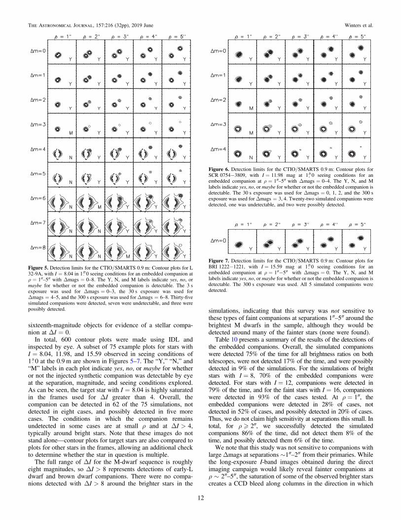
In total, 600 contour plots were made using IDL andinspected by eye. A subset of 75 example plots for stars withI=8.04, 11.98, and 15.59 observed in seeing conditions of1 0 at the 0.9 m are shown in Figures 5–7. The “Y,” “N,” and“M” labels in each plot indicate yes, no, or maybe for whetheror not the injected synthetic companion was detectable by eyeat the separation, magnitude, and seeing conditions explored.As can be seen, the target star with I=8.04 is highly saturatedin the frames used for ΔI greater than 4. Overall, thecompanion can be detected in 62 of the 75 simulations, notdetected in eight cases, and possibly detected in five morecases. The conditions in which the companion remainsundetected in some cases are at small ρ and at ΔI>4,typically around bright stars. Note that these images do notstand alone—contour plots for target stars are also compared toplots for other stars in the frames, allowing an additional checkto determine whether the star in question is multiple.

The full range of ΔI for the M-dwarf sequence is roughlyeight magnitudes, so ΔI>8 represents detections of early-Ldwarf and brown dwarf companions. There were no compa-nions detected with ΔI>8 around the brighter stars in the

simulations, indicating that this survey was not sensitive tothese types of faint companions at separations 1″–5″ around thebrightest M dwarfs in the sample, although they would bedetected around many of the fainter stars (none were found).Table 10 presents a summary of the results of the detections of

the embedded companions. Overall, the simulated companionswere detected 75% of the time for all brightness ratios on bothtelescopes, were not detected 17% of the time, and were possiblydetected in 9% of the simulations. For the simulations of brightstars with I=8, 70% of the embedded companions weredetected. For stars with I=12, companions were detected in79% of the time, and for the faint stars with I=16, companionswere detected in 93% of the cases tested. At ρ=1″, theembedded companions were detected in 28% of cases, notdetected in 52% of cases, and possibly detected in 20% of cases.Thus, we do not claim high sensitivity at separations this small. Intotal, for ρ�2″, we successfully detected the simulatedcompanions 86% of the time, did not detect them 8% of thetime, and possibly detected them 6% of the time.We note that this study was not sensitive to companions with

largeΔmags at separations ∼1″–2″from their primaries. Whilethe long-exposure I-band images obtained during the directimaging campaign would likely reveal fainter companions atρ∼2″–5″, the saturation of some of the observed brighter starscreates a CCD bleed along columns in the direction in which

Figure 5. Detection limits for the CTIO/SMARTS 0.9 m: Contour plots for L32-9A, with I=8.04 in 1 0 seeing conditions for an embedded companion atρ=1″–5″ with Δmags=0–8. The Y, N, and M labels indicate yes, no, ormaybe for whether or not the embedded companion is detectable. The 3 sexposure was used for Δmags=0–3, the 30 s exposure was used forΔmags=4–5, and the 300 s exposure was used forΔmags=6–8. Thirty-fivesimulated companions were detected, seven were undetectable, and three werepossibly detected.

Figure 6. Detection limits for the CTIO/SMARTS 0.9 m: Contour plots forSCR0754−3809, with I=11.98 mag at 1 0 seeing conditions for anembedded companion at ρ=1″–5″with Δmags=0–4. The Y, N, and Mlabels indicate yes, no, or maybe for whether or not the embedded companion isdetectable. The 30 s exposure was used for Δmags=0, 1, 2, and the 300 sexposure was used forΔmags=3, 4. Twenty-two simulated companions weredetected, one was undetectable, and two were possibly detected.

Figure 7. Detection limits for the CTIO/SMARTS 0.9 m: Contour plots forBRI1222−1221, with I=15.59 mag at 1 0 seeing conditions for anembedded companion at ρ=1″−5″ with Δmags=0. The Y, N, and Mlabels indicate yes, no, or maybe for whether or not the embedded companion isdetectable. The 300 s exposure was used. All 5 simulated companions weredetected.

12


the CCDs read out. Faint companions located within ∼1″–2″ oftheir primaries, but at a position angle near 0° or 180° would beoverwhelmed by the CCD bleed of the saturated star andnot be detected. We do not include any correction due to thisbias, as it mostly applies to companions at separations <2″from their primaries, below our stated detection limitsensitivity.

3.2.2. Detection Limits Summary

Figure 8 illustrates detected companions in the Blinking andCCD Imaging Surveys, providing a comparison for thedetection limits derived here. We note that the largest ΔIdetected was roughly 6.0 mag (GJ 752B), while the largestangular separation detected was 295″ (GJ 49B).

Figure 9 indicates the coverage curves for our two mainsurveys as a function of projected linear separation. Usingthe angular separation limits of each survey (2″–10″ for theimaging survey and 5″–300″ for the blinking survey) and thetrigonometric distances of each object to determine the upperand lower projected linear separation limit for each M-dwarfprimary in our sample, we show that either the imaging orblinking survey would have detected stellar companions atprojected distances of 50–1000 au for 100% of our sample.

3.3. Searches at Separations �2″

In addition to the blinking and CCD imaging searches,investigations for companions at separations smaller than 2″were possible using a variety of techniques, as detailed belowin Sections 3.3.1–3.3.4. The availability of accurate parallaxesfor all stars and of VRIJHK photometry for most stars madepossible the identification of overluminous red dwarfs thatcould be harboring unresolved stellar companions. Varioussubsets of the sample were also probed using long-termastrometric data for stars observed during RECONS’ astro-metry program, as well as via data reduction flags indicatingastrometric signatures of unseen companions for stars observedby Hipparcos.

3.3.1. Overluminosity via Photometry: Elevation

above the Main Sequence

Accurate parallaxes and V and K magnitudes for stars in thesample allow the plotting of the observational HR diagram

shown in Figure 10, where MV and the (V− K ) color are usedas proxies for luminosity and temperature, respectively.Unresolved companions that contribute significant flux to thephotometry cause targets to be overluminous, placing themabove the main sequence. Known multiples with separations<5″17 are evident as points clearly elevated above the

Figure 8. Log-linear plot of ΔI vs.angular separation to illustrate theobservational limits of our Blinking and CCD Imaging Surveys. Solid blackpoints indicate known companions that were confirmed, while the newcompanions discovered during our searches are shown as larger blue points.

Figure 9. Fraction of our sample surveyed as a function of log-projected linearseparation. The curve for the imaging campaign is shown as a red dotted line,while the blinking campaign coverage is shown as a blue dashed line. The solidblack line indicates the combined coverage of the two campaigns. We showthat our surveys are complete for stellar companions at projected linearseparations of roughly 50–1000 au, 75% complete at separations 40–3000 au,and 50% complete at separations 30–4000 au.

Figure 10. Observational HR diagram for 1120 M dwarf primaries, with MV

plotted vs. (V − K ) color. All primaries are plotted as black points. Overplottedare known close multiples with separations smaller than 5″ having blendedphotometry (red points), known subdwarfs (open green squares), and knownyoung objects (open cyan diamonds). Error bars are shown in gray and aresmaller than the points in most cases. The large K magnitude errors for fourobjects (GJ 408, GJ 508.2, LHS 3472, and LP 876-26AB) have been omittedfor clarity. As expected, known multiples with merged photometry are oftenelevated above the middle of the distribution. The 11 stars suspected to be newunresolved multiples due to their elevated positions relative to the mainsequence are indicated with open blue circles. The 10 stars suspected to be newunresolved multiples due to their distance mismatches from Figure 11 areindicated with open blue triangles. Note that the candidate multiples detectedby main-sequence elevation are mostly mid- to late-type M dwarfs, while thesuspected multiples identified by the distance mismatch technique are primarilyearly-type M dwarfs.

17 This 5″ separation appears to be the boundary where photometry formultiple systems from the literature—specifically from Bessell and Weis—becomes blended. For photometry available from the SAAO group (e.g.,Kilkenny, Koen), the separation is ∼10″ because they use large apertures whencalculating photometric values.

13


presumed single stars on the main sequence, and merge with afew young objects. Subdwarfs are located below and to the leftof the singles, as they are old, metal-poor, and underluminousat a given color. Eleven candidate multiples lying among thesequence of known multiples have been identified by eye viathis HR diagram. These candidates are listed in Table 12 andare marked in Figures 10 and 11. Note that these candidates areprimarily mid- to late-M dwarfs. Known young stars and

subdwarfs were identified during the literature search and arelisted in Tables 13 and 14, along with their identifyingcharacteristics. More details on these young and old systemsare given in Sections 3.4.2 and 3.4.3.

3.3.2. Overluminosity via Photometry: Trigonometric and CCD

Distance Mismatches

Because both VRI and 2MASS JHK photometry are nowavailable for nearly the entire sample, photometric distancesbased on CCD photometry (ccddist) were estimated andcompared to the accurate trigonometric distances (trigdist)available from the parallaxes. Although similar in spirit to theHR diagram test discussed above that uses V and Kphotometry, all of the VRIJHK photometry is used for eachstar to estimate the ccddist via the technique described in Henryet al. (2004), thereby leveraging additional information. Asshown in Figure 11, suspected multiples that would otherwisehave been missed due to the inner separation limit (2″) of ourmain imaging survey can be identified due to mismatches in thetwo distances. For example, an unresolved equal-magnitudebinary would have an estimated ccddist closer by a factor of 2

compared to its measured trigdist. Unresolved multiples withmore than two components, e.g., a triple system, could be evenmore overluminous, as could young, multiple systems. Bycontrast, cool subdwarfs are underluminous, and therefore theirphotometric distances are overestimated.With this method, 50 candidate multiples were revealed with

ccddists that were 2 or more times closer than their trigdists.Of these, 40 were already known to have at least one closecompanion (36 stars) or to be young (four stars), verifying thetechnique. The remaining 10 are new candidates and are listedin Table 12.

3.3.3. RECONS Perturbations

A total of 324 red dwarfs in the sample have parallaxmeasurements by RECONS, with the astrometric coveragespanning 2–16 yr. This number is slightly higher than the 308

Figure 11. Comparison of distance estimates from VRIJHK photometryvs.distances using πtrig for 1091 of the M-dwarf primaries in the sample. The29 stars with photometric distances >30 pc are not included in this plot. Errorson the distances are noted in gray. The diagonal solid line represents 1:1agreement in distances, while the dashed lines indicate the 15% uncertaintiesassociated with the CCD distance estimates from Henry et al. (2004). Thedash–dotted line traces the location where the trigonometric distance exceedsthe photometric estimate by a factor of 2 , corresponding to an equal-luminosity/mass pair of stars. Known unresolved multiples with blendedphotometry are indicated with red points. The 11 candidate unresolvedmultiples from the HR diagram in Figure 10 are enclosed with open bluecircles. The 10 new candidates that may be unresolved multiples from this plotare enclosed with open blue triangles.

Table 13

Young Members

Name # Objects R.A. Decl. μ P.A. References vtan Youth Moving References(hh:mm:ss) (dd:mm:ss) (″ yr−1

) (deg) (km s−1) Indicator Group

LTT10301AB 2 00 50 33.23 +24 49 00.9 0.203 101.9 5 11 ol Argus 3G 80-21 1 03 47 23.35 −01 58 19.8 0.323 147.8 5 25 Li AB Dor 32MA0414−0906 1 04 14 17.29 −09 06 54.3 0.168 325.2 4 19 Li none 3LP776−25 1 04 52 24.42 −16 49 22.2 0.243 150.7 2 18 ol AB Dor 3GJ2036AB 2 04 53 31.20 −55 51 37.3 0.149 060.6 5 8 BF AB Dor 3LP717−36AB 2 05 25 41.67 −09 09 12.6 0.197 164.7 6 19 ol AB Dor 3APCOL 1 06 04 52.16 −34 33 36.0 0.330 003.6 6 13 Li Argus 3CD-35 2722AB 2 06 09 19.22 −35 49 31.1 0.057 186.4 4 6 BF AB Dor 3GJ2060ABC 3 07 28 51.37 −30 14 49.2 0.212 207.9 5 15 BF AB Dor 3G 161-71 1 09 44 54.19 −12 20 54.4 0.321 277.1 1 21 ol Argus 1GJ382 1 10 12 17.67 −03 44 44.4 0.314 219.0 5 12 ol AB Dor 3TWA22AB 2 10 17 26.91 −53 54 26.5 0.149 264.4 6 12 Li Beta Pic 3GJ393 1 10 28 55.56 +00 50 27.6 0.950 219.3 5 32 ol AB Dor 3GJ490ABCD 4 12 57 40.26 +35 13 30.3 0.307 240.9 5 29 BF Tuc-Hor 3GJ856AB 2 22 23 29.08 +32 27 33.1 0.329 129.1 5 24 Li AB Dor 3GJ871.1AB 2 22 44 57.96 −33 15 01.7 0.230 123.1 5 25 (Li) Beta Pic 3HIP114066 1 23 06 04.83 +63 55 33.9 0.185 108.5 5 21 Li AB Dor 3

Note.The youth indicators are as follows: BF —a bona fide and well-known member of a moving group; Li—the presence of lithium; ol—over-luminous.References.(1) Bartlett et al. (2017); (2) Høg et al. (2000); (3) Riedel et al. (2017); (4) Shkolnik et al. (2012); (5) van Leeuwen (2007); (6) Winters et al. (2015).

14


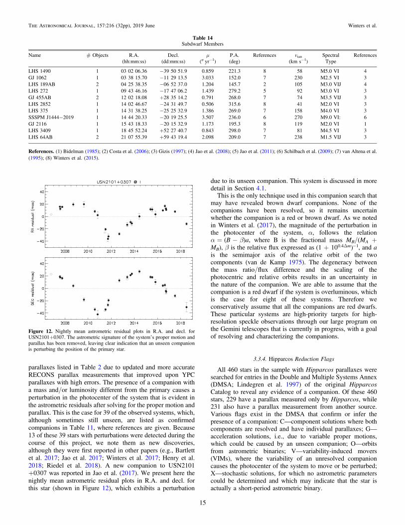
parallaxes listed in Table 2 due to updated and more accurateRECONS parallax measurements that improved upon YPCparallaxes with high errors. The presence of a companion witha mass and/or luminosity different from the primary causes aperturbation in the photocenter of the system that is evident inthe astrometric residuals after solving for the proper motion andparallax. This is the case for 39 of the observed systems, which,although sometimes still unseen, are listed as confirmedcompanions in Table 11, where references are given. Because13 of these 39 stars with perturbations were detected during thecourse of this project, we note them as new discoveries,although they were first reported in other papers (e.g., Bartlettet al. 2017; Jao et al. 2017; Winters et al. 2017; Henry et al.2018; Riedel et al. 2018). A new companion to USN2101+0307 was reported in Jao et al. (2017). We present here thenightly mean astrometric residual plots in R.A. and decl. forthis star (shown in Figure 12), which exhibits a perturbation

due to its unseen companion. This system is discussed in moredetail in Section 4.1.This is the only technique used in this companion search that

may have revealed brown dwarf companions. None of thecompanions have been resolved, so it remains uncertainwhether the companion is a red or brown dwarf. As we notedin Winters et al. (2017), the magnitude of the perturbation inthe photocenter of the system, α, follows the relationα=(B−β)a, where B is the fractional mass MB/(MA +MB), β is the relative flux expressed as 1 10 m0.4 1+ D -( ) , and a

is the semimajor axis of the relative orbit of the twocomponents (van de Kamp 1975). The degeneracy betweenthe mass ratio/flux difference and the scaling of thephotocentric and relative orbits results in an uncertainty inthe nature of the companion. We are able to assume that thecompanion is a red dwarf if the system is overluminous, whichis the case for eight of these systems. Therefore weconservatively assume that all the companions are red dwarfs.These particular systems are high-priority targets for high-resolution speckle observations through our large program onthe Gemini telescopes that is currently in progress, with a goalof resolving and characterizing the companions.

3.3.4. Hipparcos Reduction Flags

All 460 stars in the sample with Hipparcos parallaxes weresearched for entries in the Double and Multiple Systems Annex(DMSA; Lindegren et al. 1997) of the original Hipparcos

Catalog to reveal any evidence of a companion. Of these 460stars, 229 have a parallax measured only by Hipparcos, while231 also have a parallax measurement from another source.Various flags exist in the DMSA that confirm or infer thepresence of a companion: C—component solutions where bothcomponents are resolved and have individual parallaxes; G—acceleration solutions, i.e., due to variable proper motions,which could be caused by an unseen companion; O—orbitsfrom astrometric binaries; V—variability-induced movers(VIMs), where the variability of an unresolved companioncauses the photocenter of the system to move or be perturbed;X—stochastic solutions, for which no astrometric parameterscould be determined and which may indicate that the star isactually a short-period astrometric binary.

Table 14

Subdwarf Members

Name # Objects R.A. Decl. μ P.A. References vtan Spectral References(hh:mm:ss) (dd:mm:ss) (″ yr−1

) (deg) (km s−1) Type

LHS1490 1 03 02 06.36 −39 50 51.9 0.859 221.3 8 58 M5.0 VI 4GJ1062 1 03 38 15.70 −11 29 13.5 3.033 152.0 7 230 M2.5 VI 3LHS189AB 2 04 25 38.35 −06 52 37.0 1.204 145.7 2 105 M3.0 VIJ 4LHS272 1 09 43 46.16 −17 47 06.2 1.439 279.2 5 92 M3.0 VI 3GJ455AB 2 12 02 18.08 +28 35 14.2 0.791 268.0 7 74 M3.5 VIJ 3LHS2852 1 14 02 46.67 −24 31 49.7 0.506 315.6 8 41 M2.0 VI 3LHS375 1 14 31 38.25 −25 25 32.9 1.386 269.0 7 158 M4.0 VI 3SSSPMJ1444−2019 1 14 44 20.33 −20 19 25.5 3.507 236.0 6 270 M9.0 VI: 6GJ2116 1 15 43 18.33 −20 15 32.9 1.173 195.3 8 119 M2.0 VI 1LHS3409 1 18 45 52.24 +52 27 40.7 0.843 298.0 7 81 M4.5 VI 3LHS64AB 2 21 07 55.39 +59 43 19.4 2.098 209.0 7 238 M1.5 VIJ 3

References.(1) Bidelman (1985); (2) Costa et al. (2006); (3) Gizis (1997); (4) Jao et al. (2008); (5) Jao et al. (2011); (6) Schilbach et al. (2009); (7) van Altena et al.(1995); (8) Winters et al. (2015).

Figure 12. Nightly mean astrometric residual plots in R.A. and decl. forUSN2101+0307. The astrometric signature of the system’s proper motion andparallax has been removed, leaving clear indication that an unseen companionis perturbing the position of the primary star.

15


Most of the AFGK systems observed by Hipparcos that haveflags in the DMSA have been further examined or reanalyzedby Pourbaix et al. (2003, 2004), Platais et al. (2003), Jancartet al. (2005), Frankowski et al. (2007), and Horch et al.(2002, 2011a, 2011b, 2015b, 2017); however, only few of theM-dwarf systems have been investigated to date. Stars with Cand O flags were often previously known to be binary, areconsidered to be confirmed multiples, and are included inTable 11. We found that G, V, or X flags existed for 31 systemsin the survey—these suspected multiples are listed in Table 12.

3.4. Literature Search

Finally, a literature search was carried out by reviewing all1120 primaries in SIMBAD and using the available biblio-graphy tool to search for papers reporting additional compa-nions. While SIMBAD is sometimes incomplete, mostpublications reporting companions are included. Papers thatwere scrutinized in detail include those reporting high-resolution spectroscopic studies (typically radial velocity planetsearches or rotational velocity results that might reportspectroscopic binaries), parallax papers that might reportperturbations, high-resolution imaging results, speckle inter-ferometry papers, and other companion search papers. A longlist of references for multiple systems found via the literaturesearch is included in Table 11.

In addition, the Washington Double Star Catalog (WDS),maintained by Brian Mason,18 was used extensively to findpublications with information on multiple systems. Regardingthe WDS, we note that (1) not all reported companions are truephysical members of the system with which they are listed, and(2) only resolved companions (i.e., no spectroscopic orastrometric binaries) are included in the catalog. Thus, carehad to be taken when determining the true number ofcompanions in a system. Information pertaining to a star inthe WDS was usually only accessed after it was already knownthat the system was multiple and how many components werepresent in the system, so this was not really troublesome.However, the WDS sometimes had references to multiplicitypublications that SIMBAD had not listed. Thus, the WDSproved valuable in identifying references and the separations,magnitude differences, and other information included inTable 11.

Finally, all of the multiple systems were cross-checkedagainst the Gaia DR2 through the Aladin interface. Thirty-twoknown multiple systems had positional data, but no parallax,while 14 known systems were not found. Of the 575 stellarcomponents presented in this sample, 133 were not found tohave separate data points. The majority of these companionsare located at subarcsecond angular separations from theirprimaries, with a rare few having separations 1″–3″. Anadditional 15 companions had unique coordinates, but noindividual parallax or proper motion. We anticipate that futureGaia data releases will provide some of the currently missinginformation for these low-mass multiple systems.

Information for all multiple systems (including brown dwarfcomponents) is presented in Table 11, with n-1 lines for eachsystem, where n is the total number of components in thesystem. For example, a quadruple system will have three linesof information that describe the system. The name is followed

by the number of components in the system and theconfiguration map of the components detailed in that line ofthe table. If the line of data pertains to higher order systemscontaining component configurations for subsystems (e.g.,“BC” of a triple system), the number of components noted willbe “0,” as the full membership of the system will already havebeen noted in the line of data containing the “A” component.These data are followed by epoch J2000.0 coordinates, theangular separation (ρ) in arcseconds, the position angle (θ) indegrees measured east of north, the year of the measurement,the code for the technique used to identify the component, andthe reference. We assign a separation of <1″ for all astrometricand spectroscopic binaries (unless more information isavailable) and/or to indicate that a companion has beendetected, but not yet resolved. We note that where orbitdeterminations from the literature are reported, the semimajoraxis, a, is listed instead of ρ. If a was not reported in thereference given, it was calculated from the period and theestimated masses of the components in question via Kepler’sthird law.The final three columns give a magnitude difference (Δmag)

between the components indicated by the configuration map,the filter used to measure this Δmag, and the reference for thismeasurement. Photometry from photographic plates is denotedby “V*.” In many cases, there are multiple separation andΔmag measurements available in the literature from differentgroups using different techniques. An exhaustive list of theseresults is beyond the scope of this work; instead, a single recentresult for each system is listed. In a few cases, the positionangles and/or Δmag measurements are not available. Wediscuss how these systems are treated in Section 5.3.1.

3.4.1. Suspected Companions

Forty-nine singles suspected to be doubles were revealedduring this survey, three of which (GJ 912, GJ 1250, andSCR 1826−6542) have so far been confirmed with continuingfollow-up observations. An additional five doubles aresuspected to be triples, yielding a current total of 54 suspectedadditional companions (only one companion per system in allcases) listed in Table 12, but not included in Table 11.19

Systems in Table 12 are listed with the suspected number ofcomponents followed by a question mark to indicate thesystem’s suspect status, followed by J2000.0 coordinates, a flagcode for the reason a system is included as having a candidatecompanion, and the reference. Notes to the table give detaileddescriptions of the flags. Of the 56 suspected companions,31 are from the Hipparcos DMSA, in which they are assignedG, V, or X flags. A number of primaries that were suspected tobe multiple due to either an underestimated ccddist or anelevated position on the HR diagram were found through theliterature search to have already been resolved by others andhave been incorporated into Table 11 and included in theanalysis as confirmed companions. There remain 21 systems inTable 12 with ccddist values that do not match theirtrigonometric parallax distances and/or that are noticeablyelevated above the main sequence that have not yet beenconfirmed. A few more systems had other combinations ofindicators that they were multiple, e.g., an object with a

18 The primary copy is kept at USNO and a back-up copy is housed at GeorgiaState University.

19 For consistency, companions to GJ912, GJ1250, and SCR1826−6542areincluded in Table 12 and in the “Suspects” portion of the histogram inFigure 16.

16


perturbation might also have a distance mismatch. Six starswere reported as suspected binaries in the literature. GJ 207.1,GJ 341, GJ 373, GJ 1136A, and HIP 92451 were noted byReiners et al. (2012) as possible spectroscopic binaries, and GJ465 was identified by Heintz (1986) as a possible astrometricbinary. These are listed in Table 12. We reiterate that none ofthese suspected companions have been included in any of theanalyses of the previous section or that follow; only confirmedcompanions have been used.

3.4.2. Young Stellar Objects

Within the solar neighborhood are young moving groups thathave contributed members to the multiplicity sample. Withinthe studied collection are 16 confirmed young M dwarfs, 9 ofwhich are known to be multiple, yielding an MR of 56±19%.We note that this result is not statistically robust due to thesmall number of objects with which it was calculated.Presented in Table 13 are these known nearby young reddwarfs, with their astrometric data duplicated from Table 3. Inaddition, the tangential velocity vtan is listed, along with theyouth indicators, the moving group with which they areassociated, and the reference. The youth indicators are asfollows: BF—a bona fide and well-known member of a movinggroup; Li—the presence of lithium; ol—over-luminous. Anymember of a multiple system where one component exhibitsany of these indicators is also assumed to be young, as in thecase of GJ 871.1AB. We note that we do not exclude any of theidentified young M-dwarf members from our sample. Thiswould arbitrarily bias our sample, as a comprehensive searchfor these objects in the current sample has not been conducted.

3.4.3. Old, Cool Subdwarfs

There are a small number of old halo members, also knownas cool subdwarfs, that happen to be passing through the solarneighborhood. The objects have been identified either spectro-scopically or stand out on a reduced proper motion diagram.Out of the 11 confirmed subdwarf members with trigonometricparallaxes found within 25 pc, only 3 are multiple systems,resulting in an MR of 27±16%. This is very similar to that ofthe M-dwarf population as a whole (26.8± 1.4%; seeSection 5.2) and in agreement with a larger sample of 62 Kand M subdwarfs has been studied by Jao et al. (2009), whofound a rate of of 26±6%. As with the young stars, with sucha small number of objects, this result is not statistically robust.The known subdwarfs in our sample are identified in Table 14.In addition to the astrometric data for each system that havebeen duplicated from Table 3, the calculated tangentialvelocities vtan and spectral types from the literature are listed.We note that we do not exclude any of the identified M-typesubdwarfs from our study. This would arbitrarily bias oursample, as a comprehensive search for these objects in thecurrent sample has not been conducted.

3.4.4. Substellar Companions

Because this study focuses on the stellar companions of Mdwarfs, it was important to determine which companions werestellar and which were substellar. Dieterich et al. (2014) foundthat the boundary between stars and brown dwarfs is near theL2.0V spectral type; efforts are underway to determine to whatmass this spectral type corresponds. As mentioned in Section 2,MV=20.0 and (V− K )=9.5 were used as cutoffs for the

faintest and reddest (and correspondingly least massive) Mdwarfs. Analysis of the main sequence in the HR diagramcreated from the RECONS list of stars and brown dwarfswithin 25 pc indicates that MV=21.5 and V K 10.3- =( )

correspond to spectral type L2.0V, and therefore the end of thestellar main sequence. Thus, for this large statistical study, weconsider objects fainter or redder than these limits to besubstellar brown dwarfs.Via the literature search, 18 brown dwarf companions to 15

M-dwarf primaries were identified. These are noted in Table 4with a “BD” for the component in the object column (Column2). Although no comprehensive searches have been done forbrown dwarfs as companions to the 1120 M dwarfs targetedhere (including ours), we note that as currently known, the rateof M-dwarf primaries with known brown dwarf companions is1.3±0.3%. This is a factor of 21 lower than the stellar MR,considering the stellar and brown dwarf companions detectedto date. While more brown dwarf companions will undoubtedlybe found in the future, it seems that they are genuinely muchrarer than stellar companions. We note that astrometricdetection via a perturbation is the only technique used in thissurvey that was sensitive to brown dwarf companions, and onlya few stars (GJ 1215 and SCR 1845−6357) have so far beenfound to be orbited by brown dwarfs via perturbations in datafrom our astrometric survey at the CTIO/SMARTS 0.9 m.We do not include any brown dwarf companions in the

analysis that follows, nor are planetary companions addressedin this work.

4. Notes on Individual Systems

4.1. New Companions

Several new companions were discovered during thesurveys, or were confirmed after being noticed during thelong-term astrometry program at the CTIO/SMARTS 0.9 m.They are listed in order of R.A.. In each case, archivalSuperCOSMOS plates were blinked to eliminate the possibilitythat new companions were background objects.

1. GJ84.1C (0205−2804). was found during the imagingsurvey separated by 1 5 from GJ 84.1B at a positionangle of 299° and with a ΔI=0.23 mag, making thesystem a triple. The SuperCOSMOS B and R plates, taken1977 September and 1994 November, respectively,provide a Δt of 17.2 years. Blinking these two platesusing the CDS Aladin interface showed that the Bcomponent, with a proper motion of 0 549 yr−1, moved9 4. Projecting the star’s position forward 17 years to thedate of the observation (2011 October) indicates thatthere was no background star at the position of the Bcomponent at that time. Astrometry from the Gaia DR2confirms our discovery, with reported parallaxes of38.29±0.03, 38.51±0.08, and 38.15±0.10 mas forthe now three components. We therefore consider thisstar a new member of the system.

2. 2MA0936−2610C (0936−2610). During the blinkingsurvey, we detected a new companion to this previouslyknown double star at ρ=41 8, θ=315°, making this atriple system. The ΔV between the AB pair and the Ccomponent is 6.9 mag. There is no Gaia DR2 parallaxavailable for the AB pair yet, but the trigonometricdistance of 18.50±0.05 pc for the C component(54.04± 0.12 mas; Gaia Collaboration et al. 2018) is in

17


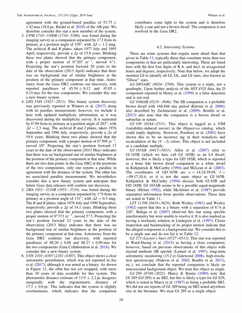
agreement with the ground-based parallax of 53.75±1.42 mas (18.6 pc; Riedel et al. 2018) of the AB pair. Wetherefore consider this star a new member of the system.

3. UPM1710−5300B (1710−5300). was found during theimaging survey as a companion separated by 1 2 from itsprimary at a position angle of 339°, with ΔI=1.2 mag.The archival B and R plates, taken 1977 July and 1993April, respectively, provide a Δt of 15.8 years. Blinkingthese two plates showed that the primary component,with a proper motion of 0 207 yr−1, moved 4 1.Projecting the star’s position forward 20 years to thedate of the observation (2013 April) indicates that therewas no background star of similar brightness at theposition of the primary component at that time. Astro-metry from the Gaia DR2 confirms our discovery, withreported parallaxes of 45.54±0.12 and 45.05±0.15 mas for the two components. We consider this stara new binary system.

4. LHS5348 (1927−2811). This binary system discoverywas previously reported in Winters et al. (2017) alongwith its parallax measurement; however, we include ithere with updated multiplicity information, as it wasdiscovered during the multiplicity survey. It is separatedby 0 89 from its primary at a position angle of 283°, withΔI=2.3 mag. The archival B and I plates, taken 1976September and 1996 July, respectively, provide a Δt of19.8 years. Blinking these two plates showed that theprimary component, with a proper motion of 0 509 yr−1,moved 10″. Projecting the star’s position forward 17years to the date of the observation (2013 May) indicatesthat there was no background star of similar brightness atthe position of the primary component at that time. Whilethere are two data points in the Gaia DR2 at the positionsof the two components, only one reports a parallax inagreement with the distance of the system. The other hasno associated parallax measurement. We neverthelessconsider this a new binary system and anticipate thatfuture Gaia data releases will confirm our discovery.

5. 2MA1951−3510B (1951−3510). was found during theimaging survey as a companion separated by 1 9 from itsprimary at a position angle of 131°, with ΔI=0.3 mag.The B and R plates, taken 1976 July and 1990 September,respectively, provide a Δt of 14.1 years. Blinking thesetwo plates showed that the primary component, with aproper motion of 0 373 yr−1, moved 5 3. Projecting thestar’s position forward 23 years to the date of theobservation (2013 May) indicates that there was nobackground star of similar brightness at the position ofthe primary component at that time. Astrometry from theGaia DR2 confirms our discovery, with reportedparallaxes of 88.20±0.08 and 88.27±0.09 mas forthe two components (Gaia Collaboration et al. 2018). Weconsider this a new binary system.

6. USN2101+0307 (2101+0307). This object shows a clearastrometric perturbation, which was not reported in Jaoet al. (2017), although it was noted as a binary. As shownin Figure 12, the orbit has not yet wrapped, with morethan 10 years of data available for this system. Thephotometric distance estimate of 13.9±2.2 pc disagreesmarginally with the trigonometric distance of17.7±0.6 pc. This indicates that the system is slightlyoverluminous, which indicates that the companion

contributes some light to the system and is thereforelikely a star and not a brown dwarf. The companion is notresolved in the Gaia DR2.

4.2. Interesting Systems

There are some systems that require more detail than thatgiven in Table 11, typically those that constitute more than twocomponents or that are particularly interesting. These are listedhere with the first four digits of R.A. and decl. in sexagesimalhours and degrees, respectively. Note that below, we adopt themoniker GJ to identify all Gl, GL, and GJ stars, also known as“Gliese” stars.GJ2005ABC (0024−2708). This system is a triple, not a

quadruple. Upon further analysis of the HST-FGS data, the Dcomponent reported in Henry et al. (1999) is a false detectionand is not real.GJ1046AB (0219−3646). The SB companion is a probable

brown dwarf with 168.848 -day period (Kürster et al. 2008);also described by Zechmeister et al. (2009). Bonfils et al.(2013) also note that the companion is a brown dwarf orsubstellar in nature.GJ109 (0244+2531). This object is tagged as a VIM

(variability-induced mover) in the Hipparcos catalog, whichcould imply duplicity. However, Pourbaix et al. (2003) haveshown this to be an incorrect tag in their reanalysis andrecalculation of the (V− I) colors. This object is not includedas a candidate multiple.GJ165AB (0413+5031). Allen et al. (2007) refer to

Gl165B (which we here call GJ 165B) as an L4 dwarf;however, this is likely a typo for GD165B, which is reportedas a bona fide brown dwarf companion to a white dwarfin Kirkpatrick & McCarthy (1994) and McLean et al. (2003).The coordinates of GD165B are α=14:24:39.09, δ=+09:17:10.4, so it is not the same object as GJ165B.Kirkpatrick & McCarthy (1994) discuss both Gl65B andGD165B. GJ165AB seems to be a possible equal-magnitudebinary (Heintz 1992), while McAlister et al. (1987) provideseparation information from speckle observations. These dataare noted in Table 11.LTT11399 (0419+3629). Both Worley (1961) and Worley

(1962) report that this is a binary with a separation of 6 4 at226°. Balega et al. (2007) observed this star using speckleinterferometry but were unable to resolve it. It is also marked ashaving a stochastic solution in Lindegren et al. (1997). Closerinspection and backtracking of its proper motion indicate thatthe alleged component is a background star. We consider this tobe a single star and do not list it in Table 12.GJ273 (Luyten’s Star) (0727+0513). This star was reported

in Ward-Duong et al. (2015) as having a close companion;however, based on previous observations of this object withmyriad methods (IR speckle (Leinert et al. 1997), long-termastrometric monitoring (15.2 yr Gatewood 2008), high-resolu-tion spectroscopy (Nidever et al. 2002; Bonfils et al. 2013),etc.), we conclude that the reported companion is likely anunassociated background object. We treat this object as single.GJ289 (0748+2022). Marcy & Benitz (1989) note that

Gl289 (GJ 289) is an SB2, but this is likely a typo for GJ829,which is noted in Marcy et al. (1987) as being a probable SB2.We did not see reports of GJ289 being an SB2 noted anywhereelse in the literature. We treat GJ289 as a single object.

18


GJ1103 (0751−0000). Reiners et al. (2012) cite Delfosseet al. (1998) for GJ1103(A) being an SB. However, Delfosseet al. (1998) note only that they exclude GJ1103 from theirsample due to it being a binary. They do not claim that it is anSB. In the LHS Catalog (Luyten 1979a), where it is listed asLHS1951, it is advertised to have a companion LHS1952with a separation of 3″ at θ=78°, with componentmagnitudes of mR=13.0 and 15.5, and mpg=15.0 and17.5. We searched for the companion by examining bothRECONS astrometry frames, in which the seeing was some-times 1 2 or better; and via the blinking campaign. Nocompanion was found. We conclude that GJ1103 is single.

GJ450 (1151+3516). This object was reported as a low-probability binary candidate with a low-velocity amplitude byYoung et al. (1987), who measured five epochs of preciseradial velocities. However, more recent high-resolution obser-vations with ELODIE and SOPHIE over a range of resolutions(R=40,000–75,000) make no mention of this object beingmultiple (Houdebine 2010), nor was a companion detected withlucky imaging (Jódar et al. 2013) or with infrared adaptiveoptics observations (Ward-Duong et al. 2015). We thereforeconsider this object to be single.

GJ452 (1153−0722). Gould & Chanamé (2004) report alikely white dwarf companion at ρ=9″ and θ=110°that wasdetected in 1960 by Luyten (1980a). However, blinkingSuperCOSMOS plate images (epochs 1984–1997) with the300-second integration taken at the CTIO/SMARTS 0.9 mreveals no co-moving companion. Backtracking the propermotion of the star to epoch 1960 places a background star at theappropriate separation and position angle of the reportedcompanion. We thus consider this object to be single.

GJ1155AB (1216+0258). This object was previouslythought to have a white dwarf companion, but Gianninaset al. (2011) report that the white dwarf is actually amisclassified M dwarf. A survey of SDSS objects by Kleinmanet al. (2004) did not spectroscopically confirm the companionas a white dwarf. We therefore consider the companion to be anM dwarf.

GJ465 (1224−1814). Heintz (1986) notes this object mayyet be a long-term binary. We note this system as a candidatemultiple in Table 12.

GJ471 (1231+0848). Poveda et al. (1994) report that thisobject is a CPM companion to the binary GJ469AB with aseparation of 2490″. While the weighted mean trigonometricdistances from van Altena et al. (1995) and van Leeuwen(2007) agree within the error bars (73.13± 1.28 mas for GJ 471versus 74.77± 3.39 mas for GJ 469AB), their proper motionsare significantly different: 822 mas yr−1 at θ=231° forGJ471 versus 685 mas yr−1 at θ=248° for GJ469AB. Thus,we consider GJ471 a single star.

GJ477AB (1235−4556). This object is flagged in theHipparcos DMSA (Lindegren et al. 1997) as having astochastic solution, indicating that it is a probable short-periodastrometric binary. Zechmeister et al. (2009) note it as an SB1using VLT+UVES, with the companion being low-mass or abrown dwarf. We treat the companion as a stellar component.

GJ1167 (1309+2859). Jahreiß et al. (2008) note a Bcomponent with μ=0 292 yr−1, θ=234°.9, but then notethat the two stars are not physically associated, as thephotometric distance for B is 190 pc while the trigonometricdistance for A is 12 pc. We calculate the ccddist for A to be14.2 pc. Janson et al. (2012) note that A is single in their

survey. We conclude that GJ1167“B” is not a CPMcompanion to GJ1167A and that GJ1167 is a single system.GJ541.2AB (1417+4526). This system had too small a

proper motion (47 mas yr−1 at a position angle of 109.8°; vanLeeuwen 2007) to confirm its secondary component with aseparation of 55 2 at a position angle of 204°. Our image,taken in 2013, provided 18 years of coverage when blinkedwith the 1995 SuperCOSMOS plate, but resulted in the systemmoving less than an arcsecond during our blinking survey.However, the Gaia DR2 catalog confirms this system as abinary, reporting parallaxes and proper motions for bothcomponents that agree both with each other and the HIPparallax of 52.60±1.25 mas: πA=51.43±0.03 mas andμA=47.3 mas yr−1, θA=113°; πB=51.74±0.16 mas andμB=47.8 mas yr−1, θB=113°. We therefore treat this systemas binary.GJ680 (1735−4840). A companion at ρ=3 94,

θ=323°.7 with ΔH=1.93 mag was reported in Ward-Duong et al. (2015). However, while performing PSFphotometry in the crowded field in order to deblend themagnitudes of the primary and secondary, we noted that thealleged secondary had not moved with the primary betweenepochs of photometry taken 18 months apart. With a propermotion of 462 mas yr−1, the two stars would have moved apixel and a half. This was the case with the primary, but not thealleged secondary. Therefore, we deem the companion abackground star and not physically associated.GJ687 (1736+6820). Montet et al. (2014) cite Jenkins et al.

(2009) for the M3.5 companion that they note in their Table 2,but the spectral type of the primary is M3.5. Jenkins et al.(2009) do not note any additional information about acompanion.We find that the WDS lists GJ687 as the B component to

the F5 star HD160861. The parallax for the F5 star is11.20 mas (89 pc; van Leeuwen 2007), which places this objectat a much larger distance than the M dwarf, which hasπ=220.47 mas (4.5 pc; van Altena et al. 1995; van Leeu-wen 2007). It appears that the “A” component, the F5 star (atα=17:36:42, δ=+68:22:59, compared to α=17:36:25.9,δ=+68:20:20 for GJ 687) is an SB, for which the measure-ment by McAlister et al. (1987) pertains. Tokovinin (1992)notes GJ687 as both an astrometric and speckle binary in thetable in that paper named “Long-period spectroscopic bin-aries.” This, too, is likely for the F dwarf, however. Thecompanion is deemed to be optical, and we consider GJ687 tobe single.LTT15769 (1945+3223). This system is listed as double in

the Hipparcos DMSA (Lindegren et al. 1997) with ρ=12 76,θ=339° with a quality code of “D,” indicating an uncertainsolution. Blinking the SuperCOSMOS R plate image with an I-band image taken with the Lowell 42-inch image results in anepoch difference of 19 years and reveals the motion of theprimary, but not that of the bright “secondary” with a ΔHp of2.3 mag. We thus refute this low-probability companion anddeem the system “single.”GJ793 (2030+6527). Weis (1991b) lists this object in the

“Rejected Pairs” table (Table 5) and note that the allegedcompanion is not listed in either the Luyten or Giclas catalogs.The SuperCOSMOS photographic plates had an epoch spreadof only one year, so we used the 300 s image taken during ourimaging campaign at the Lowell 42-inch telescope to blinkwith the SuperCOSMOS I-band archival image. This resulted

19


in a δt=20 yr. No CPM companion was detected. We confirmthat this object is single.

GJ873 (2246+4420). This object was reported by van deKamp & Worth (1972) to be an astrometric binary, but thisdetection was later found to be due to systemmatic errors in themicrometric separation measurements (Heintz 1976).

Young et al. (1987) initially report this object as a high-probability SB1, but then note in the appendix to that paper thatthe detection is tentative due to the low-velocity amplitude ofthe signal.

Hełminiak et al. (2009) also investigate this system, citing a“B” component that they infer is a real binary with spectral typeG, but not associated with the “A” component, our M dwarf.We confirm by blinking that the two are not physically boundbecause the G-dwarf binary has a very different proper motion(αμ=8.6 mas, δμ=−2.0 mas) from that of the M-dwarfcomponent (αμ=−705 mas, δμ=−461 mas), and thus thetwo systems do not move together. In addition, the Vmagnitudes for the two “components” are not physicallypossible if they are located at similar distances: the M dwarfhas V=10.22, while the G dwarf has V=10.66.

Tanner et al. (2010) report two unconfirmed companionsfound via AO, but the two candidates are too faint to have2MASS magnitudes available.

Finally, Docobo et al. (2010) observed this object usingspeckle interferometry on a 6 m telescope and did not resolve acompanion. They were able to resolve companions down toangular separations of 22 mas, corresponding to 0.11 au at theobject’s distance of 5 pc.

We consider this object to be a single star.

5. Overall Results

We first report the multiplicity and companion rates for the1120 M dwarfs surveyed before any corrections are applied.The MR is the percentage of all systems that are multiple,regardless of whether the system is double, triple, or higherorder. For example, discovering that a member of a binarysystem has an additional close companion makes the system atriple, but would not affect the MR. The companion rate (CR)is the average number of companions per primary in thesample, so higher order multiples do affect this rate, as they adda companion to the statistics. The equations describing thesepercentages are given below, where NS is the number ofsingles, ND is the number of doubles, NT is the number oftriples, NQd is the number of quadruples, and NQn is the numberof quintuples, the highest order multiples so far known amongM-dwarf primaries within 25 pc. The denominator in both casesis 1120.

N N N N

N N N N NMR 100 1

D T Qd Qn

S D T Qd Qn

= *+ + +

+ + + +( )

N N N N

N N N N NCR 100

2 3 4. 2

D T Qd Qn

S D T Qd Qn

= *+ + ++ + + +

( )

We analyze all companions in relation to the primary of thesystem, even if they are members of sub-binaries or -triples.

5.1. Uncorrected Multiplicity and Companion Rates forConfirmed Companions

Among the 1120 M dwarfs searched, there are 265 multiplesystems with 310 new and confirmed stellar companions to

their primaries, resulting in an initial uncorrected MR ofMR=23.7±1.3% and an uncorrected stellar companion rateof CR=27.7±1.3%. The ratios of singles:doubles:triples:higher order systems is 856:223:37:3, corresponding to76:20:3:0.3%. For comparison, Raghavan et al. (2010) found56:33:8:3% for singles:doubles:triples:higher order systems forcompanions (including brown dwarfs) in a sample of 454 solar-type stars. If we include the known brown dwarf companions toM dwarfs, the ratios change only slightly, to 844:230:41:2:2,corresponding to 75:21:4:0.3%.

5.2. Adjustment to the Multiplicity and Companion Rates atSmall Separations

Because this survey was not uniformly sensitive to systemswith companions at ρ<2″, a correction should be made inorder to determine a final MR. The sample of M dwarfs within10 pc appears to be at least 90% complete based on decades ofRECONS work. Thus, this volume-limited 10 pc sampleprovides a reasonably complete set of stars that can provideinsight into the stellar CR at small separations. If effectively allof the primaries have been targeted by some type of high-resolution technique, an adjustment based on the stellar MR ofthose objects for the closest companions can be determined andapplied to the sample of 1120 M dwarfs in the full surveyoutlined here. We note that 2″ separations correspond to 20 auat 10 pc, but to 50 au at 25 pc. Thus, we perform the correctionbased on a 50 au separation.A literature search for spectroscopic and high-resolution

imaging studies targeting M dwarfs within 10 pc wasperformed to determine the companion population at smallseparations. These two techniques cover most of the separationphase space for stellar companions at separations ρ<50 au. Itwas found that all but two systems either already had a closecompanion at ρ<50 au, or had been observed with high-resolution techniques, e.g., spectroscopy, HST imaging,speckle interferometry, lucky imaging, or long-term astrome-try. Because 186 of the 188 M dwarfs within 10 pc have beensearched, we infer that we can use the 10 pc sample to correctfor unresolved companions with ρ<50 au at distances10–25 pc.Figure 13 presents a graph of the running stellar multiplicity

at different angular and projected linear separations as afunction of distance for the sample of M dwarfs found within25 pc. For the 13 M dwarfs with only substellar companions,the system was considered single for the purpose of the stellarmultiplicity calculation, while the two systems that had both anM dwarf and a substellar companion were considered multiple.For higher order multiple systems with more than onecompanion, the smallest separation between the primary anda companion was chosen to mitigate the likely incompletenessat small ρ in the top panel. All stellar companions at allseparations are included in the bottom panel.The striking feature of Figure 13 (top) is that most stellar

companions to red dwarfs are found at angular separationssmaller than 2″ (50 au). Thus, it is not surprising that the twomain campaigns for detecting companions undertaken hereyielded few new objects, yet those searches needed to be donesystematically. It is evident that the two sets of companions atseparations greater than 2″ are effectively constant from 10 to25 pc, indicating that there are not significant numbers ofoverlooked companions at large separations from theirprimaries. The MRs for companions with angular separations

20


2″–10″ and >10″ are 3.2% and 4.7%, respectively, indicatingthat only 7.9±0.8% of the nearest M dwarfs have companionsbeyond 2″. In contrast, the curve for companions withseparations smaller than 2″ decreases from 10 to 25 pc,implying that more close companions remain to be found from10 to 25 pc. Many of these are presumably the candidatesdiscussed in Section 3.4.1 and listed in Table 12.

The bottom panel illustrates the cumulative MR subdividedinto projected linear separations smaller than and greater than50 au. Neither curve is flat. A decreasing trend is evident in thecurve showing separations <50 au, illustrating that multiplesystems are missing at those separations. An increasing trend inthe >50 au curve hints that multiple systems are missing atlarge separations as well; however, this corresponds to one

missing companion, which is within the errors of our correction(as described below), so we do not apply a correction for this.By comparing the MR for ρ<50 au at 10 pc (38/188=

20.2± 2.9%) to the rate at 10–25 pc (153/932=16.4± 1.2%),we find a correction of an additional 3.8±0.6% multiple systemsthat can be appropriately applied to stars from 10 to 25 pc. Thiscorresponds to 35 multiple systems among the 932 stars in thisshell, bringing the total number of M-dwarf multiples within 25 pcto 265 + 35=300 for 1120 primaries. Thus, the corrected MRfor the entire sample is 26.8±1.4%, indicating that roughlythree-quarters of M dwarfs are single, compared to only half ofsolar-type stars.We use the same method to calculate the correction to the

CR and find a CR of 23.9±3.1% at 10 pc and a correction of5.7±0.8%. The correction corresponds to 53 missingcompanions to the 932 primaries at 10–25 pc. This brings thetotal number of companions to 310+53=363 for 1120primaries and results in a corrected CR of 32.4±1.4%.Thus, M dwarfs have an MR of 20.2±1.2% and a CR of

23.9±1.4% at separations smaller than 50 au.We note that we have identified 56 candidate multiple

systems, 51 of which are currently believed to be single;the other 5 are already known to have a companion at alarge angular separation. An additional 4 of these 51 candidatesare located within 10 pc. All 4 have been observed with bothhigh-resolution spectroscopy and imaging, with no companionsdetected. If any are found to have a companion, the correctionwill change, but that appears unlikely to happen.

5.3. Masses for Red Dwarfs in the Sample

In order to perform any quantitative analysis of themultiplicity results related to stellar mass, a conversion fromMV to mass using an MLR was necessary for each primary andstellar companion in the sample. For single M dwarfs or widebinaries with separate V photometry, this is straightforward. Formultiples with separations smaller than roughly 4″, systemphotometry was deblended at V using PSF fits. For multiplestoo close for PSF photometry, estimates of the Δmags weremade based on the information available in the literature.

5.3.1. Deblending Photometry

For systems with companions at separations too small(typically 1″–4″) to perform effective aperture correctionphotometry, PSF photometry was performed on framesacquired in Arizona and Chile during the imaging program inorder to measure ΔV for each system. First, the contributionfrom the sky background was calculated from a “blank” part ofthe image. The region around the close pair being analyzed wasthen cropped to contain only the relevant pair, and thebackground subtracted. A Moffat curve was fit to the PSF ofthe primary, the flux determined from the fit, and then theprimary was subtracted from the image, with care taken tominimize the residual counts from the primary. Gaussian andLorentzian curves were also tested, but it was found that Moffatcurves provided the best fits to PSFs from all of the 1meter-class telescopes used in this program. A Moffat curve was thenfit to the secondary component’s PSF and the flux calculatedfrom the fit. The ratio of the fluxes (fr) of the primary andsecondary yielded the ΔV (ΔV=−2.5log( fr)), which whencombined with the composite V photometry, provided the

Figure 13. Cumulative multiplicity rate at different angular (top) and projectedlinear (bottom) separations for the 265 multiples among 1120 M-dwarfsystems, binned by 1 pc and subdivided into separations of ρ<2″,2″<ρ<10″, and ρ>10″ (top) and separations of ρ<50 au andρ>50 au (bottom). The two rates for companions with separations greaterthan 2″ remain fairly constant from 10 to 25 pc, while the rate for separationssmaller than 2″ decreases slightly from ∼10 to 25 pc, and particularly from 13to 25 pc, indicating that a correction is warranted. The bottom panel shows thetranslation of angular into projected linear separations, which emphasizes thedecreasing trend at ρ<50 au. Neither suspected nor substellar companions areincluded in these graphs. The dotted lines indicate the binomial errors on eachline. The large scatter and errors on the curves at distances less than 10 pc aredue to small samples of stars.

21


individual V magnitudes (VB= VAB+ 2.5log(1+ 100.4ΔV);

V V VA B= - D ) needed to estimate masses for each comp-onent in a multiple system.

For triples where all three components were closer than 4″,the pair with the widest separation was deblended first usingthe appropriate ΔV to calculate the deblended V magnitudefor the single and the resulting pair. Then the ΔV relevant tothe remaining pair was used to calculate individual Vmagnitudes for the components of the closest pair.

For the 96 close multiples with Δmags reported in theliterature that were not in the V band, the relations reported inRiedel et al. (2014) were used to convert ΔRKC, ΔIKC, Δi′, or2MASS ΔJ, ΔH, ΔK filters to ΔVJ. Magnitude differences inthe Hipparcos Hp filter were considered to be equivalent tomagnitude differences in VJ, as were any visual Δmagsreported in the literature, e.g., those from any binary papersbefore ∼1995 that used photographic plates. For results usingthe Differential Speckle Survey Instrument (DSSI; Horch et al.2009) reported in Horch et al. (2011a, 2012, 2015a), Δ562 wasadopted to be ΔV and Δ692 was adopted to be ΔR. Horchet al. (2009) state that the 562 and 692 nm DSSI filters’ centralwavelengths are close to those of the V and R of the JohnsonUBVRI system. For observations from the RIT-Yale Tip-tiltSpeckle Imager (RYTSI; Meyer et al. 2006) reported in Horchet al. (2010, 2012), Δ550 measurements were adopted as ΔV,Δ698 were adopted as ΔR, and Δ754 nm measurements wereadopted as ΔI. The Δ814 measurements reported in Reid et al.(2001) were assumed to be ΔI. For HST NICMOS data, themean of the Δmags in the F M207 and F M222 filters wereconsidered equivalent to ΔKs. We note that we considerthe Δmags in these specific filters to be equivalent, not theindividual component magnitudes themselves. As an example,we show in Figure 14 the good agreement between the ΔHp

and ΔVJ magnitudes.We note that for pairs with ΔV values higher than 3.0, the

mass of the primary was calculated using the observed Vmagnitude as if it were single, as a companion with that ΔVcontributes negligible flux (∼6% or less) to the system.Although the ΔVs are often not well defined at differences thislarge, the ΔV was simply added to the V magnitude of theprimary and the mass estimated for the companion using that V.

The 43 pairs with unknown magnitude differences betweenthe components (i.e., typically those with separations <1″)

required estimates of theΔmag. For double-lined spectroscopicbinaries (SB2s), the secondary component would need tocontribute enough light to be able to see its spectral lines,making the system overluminous and underestimating thephotometric distance. Therefore, if the trigdist was more than1.4 times more distant than the ccddist, we adopted aΔmag=0.5; if the trigonometric distance trigdist was1.3–1.4 times more distant than the photometric distanceccddist, we adopted a Δmag=1.0. Single-lined spectroscopicbinaries (SB1s) and unresolved astrometric detections weretreated identically. If the trigdist was larger than 1.3 times theccddist, we adopted a Δmag=2.0, inferring that light fromthe secondary component contributed to the photometry of thesystem; and if the trigdist was <1.3 times the ccddist, weadopted a Δmag=3.0, as the companion did not appear tocontribute light to the system. These estimates were all done forthe filter in which the observations were done or reported; forexample, an object being observed in the I band that was notedto have an astrometric perturbation was assigned a ΔI=3,which was then converted to ΔV, as long as its two distancesagreed.The ΔV and deblended V magnitudes for the individual

components of multiple systems are given in Table 4, with anote if any of the aforementioned assumptions or conversionswere made. This is the case for slightly fewer than half (138) ofthe pairs. We note that while some of the current ΔV estimatesare imperfect, the only way to aquire masses of these systems’components is to measure their orbits, which was not a goal ofthis project.

5.3.2. Estimating Masses

A robust MLR for red dwarfs has recently been provided byBenedict et al. (2016), using extensive sets of HST-FGS andradial velocity data. We use their results on 47 stars withmasses 0.07–0.62 Me (average errors of 0.005 Me) to estimatemasses for the red dwarfs in the survey outlined here. Usingtheir mass–MV relation, which has a scatter of 0.017 Me, themassive end of the M dwarf spectral sequence for which wehave adopted MV=8.8 corresponds to 0.63 Me. The leastmassive M dwarf with MV=20.0 results in a mass of 0.075Me, consistent with the lowest mass M dwarf in Benedict et al.(2016), GJ 1245C with mass=0.076±0.001 Me.For the 24 systems with orbits presented in the literature that

reported masses for individual components, these were used“as is,” as long as the masses were true masses and notminimum masses, i.e., Msin3 i. In the nine cases whereMsin3 i was reported, we used the composite V-bandphotometry for the system, in combination with the mass ratio(M i M isin sin2

31

3 ), to estimate the ΔV between the compo-nents. While the inclination of the system is not known, it is notneeded, as the mass ratio remains the same regardless ofinclination. However, the relation between the magnitudedifference and mass ratio of the components is not linear (e.g.,see Benedict et al. 2016) and will change with primary mass.We first assumed an initial ΔV to deblend the photometryof the components. We then used the parallax to calculatethe absolute V-band photometry of each component. Finally,we used the MLR to estimate individual masses from thedeblended photometry of the components and calculatedthe mass ratio. We iterated these steps, revising the ΔV, untilthe estimated mass ratio matched that reported in the literature

Figure 14. Magnitude differences as a function of color for 12 common propermotion pairs with HIP parallaxes and individual VJ, Hp, and Ks for eachcomponent. The dot–dashed line indicates a one-to-one relation. Illustrated isthe good agreement between the ΔHp and ΔVJ for each pair.

22


for the system. The resulting ΔV estimates and masses arelisted in Table 4.

Twenty-nine of the objects in our survey had massespresented in Benedict et al. (2016) that were used to define theMLR. This provides an opportunity to assess the accuracy ofthe mass estimates assigned here. We find a mean absolutedeviation between the measured masses and our estimates of10.5%, differences that can be attributed to cosmic scatter, asdiscussed in Benedict et al. (2016). Mass estimates for allcomponents are listed in Table 4.

5.3.3. Mass Ratios

With mass estimates for all the stars in multiple systems inhand, we can evaluate the mass ratios of all companionsrelative to their primaries. Figure 15 shows the distribution ofthe mass ratios (q=Mcomp/Mpri) for the 310 pairs in thesample. All companions were analyzed in relation to theprimary of the system. There are 225 binaries, as well as 37triples that result in 74 pairs of objects, one quadruple systemyielding 3 pairs, and the two quintuple systems yielding 8 pairs.In the instances where Δmags reported in the literature forhierarchical systems was other than with respect to the “A”component, these data were calculated by first deblending thepair in question, calculating individual magnitudes, estimatingindividual masses, and then calculating the mass ratios inrelation to the primary.

As shown in Figure 15, most of the pairs in the sample havemass ratios higher than 0.5 with a distribution that may verywell be flat from q=0.5–1.0. Once accurate mass determina-tions are available for the pairs represented in red in thehistogram (primarily spectroscopic and astrometric binaries),the distribution may shift leftward somewhat, as we haveassumed a conservative ΔV of 3 mag for some of these targets.For q<0.5, there are a few incompleteness effects. First, wehave excluded from the analysis the 18 known brown dwarfcompanions, which affect mass ratio evaluations more for Mdwarfs than for any other type of star. Second, we show inSection 2.2 that primaries with masses 0.075–0.30 Me likelyhave companions that have eluded detection. These missing

companions might fill in various parts of the distribution, butonly for q>0.25 (0.075 Me/0.30 Me), where 0.25 is thelowest q value possible in that mass regime when consideringonly stellar companions.In order to assess whether the trend from q=0.5–1.0 is real

or due to a bias in the way the ΔV values were calculated (asdescribed above), the histogram has been color-coded in orderto identify any trends: blue represents pairs with Δmag in V(172 pairs), green represents pairs for which a conversion froma Δmag other than ΔV was made (96 pairs), and red representspairs for which an assumption had to be made about the Δmagbetween the two components, e.g., unresolved spectroscopicand astrometric binaries (43 pairs). We do not see any strongsystematic trend that correlates with the assumptions orconversions that were used for the mass estimates.

5.4. The Separation Distribution for the Nearby M Dwarfs

Figure 16 illustrates the projected separations of the 290confirmed, 20 new, and 56 suspected stellar companions fromtheir primaries. A Gaussian curve has been fit to thedistribution of confirmed and new (but not suspected)companions as a function of log-separation, providing areasonable fit to the distribution as known in the current dataset. Exoploration of fitting a skewed Gaussian curve to the dataresulted in a skew value very close to zero, with a peak at20 au. Therefore, we justify our use of a normal Gaussian curvein this analysis. In an even larger sample that has beencompletely searched for companions at small separations, adifferent distribution may prove to be more appropriate.The peak in the separation distribution of our sample falls at

20 au, with a broad spread. This distribution peaks at largerprojected separations than the one presented in Janson et al.(2014a) for mid-type M dwarfs (6 au, their Figure 3). However,their search was for companions at angular separations0 08–6″ from their primaries at inferred distances within52 pc (corresponding to 4–312 au), whereas our study searchedfor companions at angular separations out to 300″, corresp-onding to separations as large as 7500 au at the survey horizonof 25 pc. In addition, their results are based on a sample

Figure 15. Histogram of the distribution of the mass ratios (M2/M1, M3/M1,etc.) of the 310 stellar pairs in the sample. In blue are plotted pairs for which noconversion or assumption to ΔV was made, green indicates a conversion to ΔV

from another filter, and red indicates that an assumption was made regardingthe Δmag. The distribution is likely incomplete at mass ratios lower than 0.5and uniform from 0.5 to equal-mass ratios of 1.0, as the red shaded portions ofthe histogram will likely shift leftward in the future once more accurate massmeasurements are available. We note that no corrections due to “missing”multiple systems have been incorporated into this distribution, nor are browndwarf companions included.

Figure 16. Histogram of the distribution of the projected separations of allstellar companions from their red dwarf primaries, in log form. The 290confirmed (in red), 20 new (in blue), and 56 suspected companions (in green)are indicated. The dashed curve is a Gaussian that has been fit to thedistribution of confirmed and new (but not suspected) companions and has apeak at 20 au, with σlog a=1.16. The dot–dashed line is a fit to the 56M-dwarf pairs within 10 pc, denoted by the black outline, indicating a peak at4 au. For comparison, the dotted line indicates the fit for solar-type stars fromRaghavan et al. (2010), which peaks at 51 au or log P=5.03, withσlog P=2.28 yr.

23


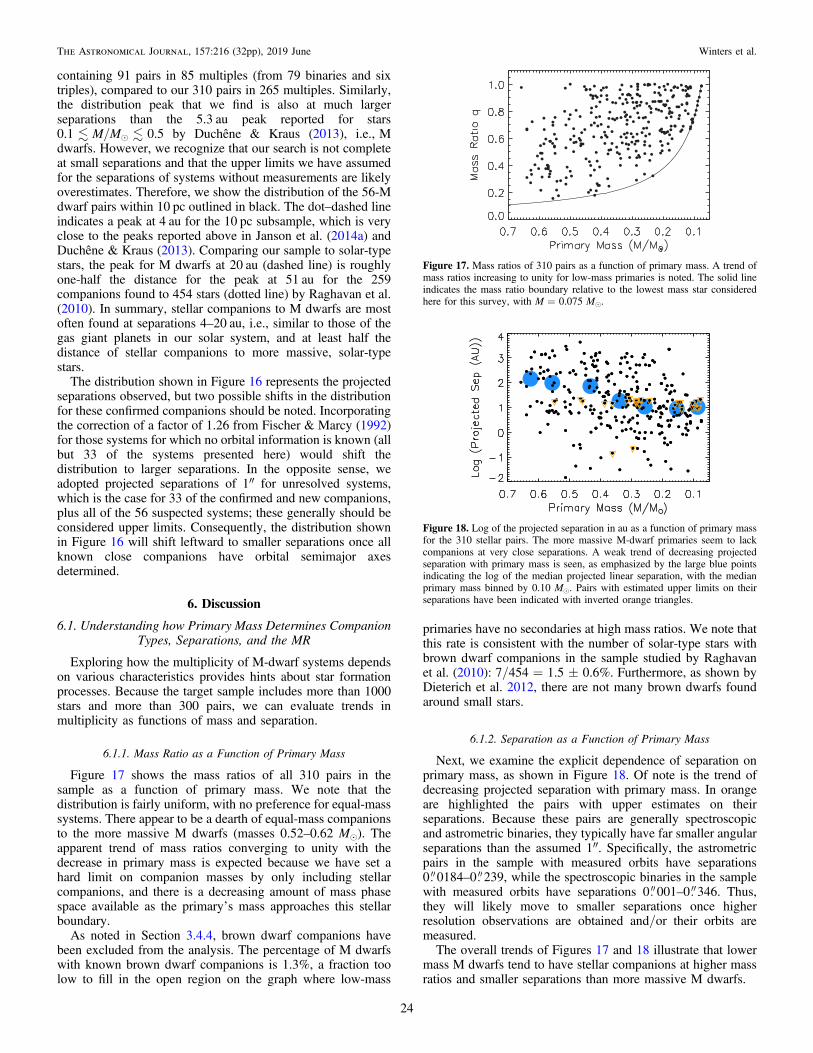
containing 91 pairs in 85 multiples (from 79 binaries and sixtriples), compared to our 310 pairs in 265 multiples. Similarly,the distribution peak that we find is also at much largerseparations than the 5.3 au peak reported for stars0.1M/Me0.5 by Duchêne & Kraus (2013), i.e.,Mdwarfs. However, we recognize that our search is not completeat small separations and that the upper limits we have assumedfor the separations of systems without measurements are likelyoverestimates. Therefore, we show the distribution of the 56-Mdwarf pairs within 10 pc outlined in black. The dot–dashed lineindicates a peak at 4 au for the 10 pc subsample, which is veryclose to the peaks reported above in Janson et al. (2014a) andDuchêne & Kraus (2013). Comparing our sample to solar-typestars, the peak for M dwarfs at 20 au (dashed line) is roughlyone-half the distance for the peak at 51 au for the 259companions found to 454 stars (dotted line) by Raghavan et al.(2010). In summary, stellar companions to M dwarfs are mostoften found at separations 4–20 au, i.e., similar to those of thegas giant planets in our solar system, and at least half thedistance of stellar companions to more massive, solar-typestars.

The distribution shown in Figure 16 represents the projectedseparations observed, but two possible shifts in the distributionfor these confirmed companions should be noted. Incorporatingthe correction of a factor of 1.26 from Fischer & Marcy (1992)for those systems for which no orbital information is known (allbut 33 of the systems presented here) would shift thedistribution to larger separations. In the opposite sense, weadopted projected separations of 1″ for unresolved systems,which is the case for 33 of the confirmed and new companions,plus all of the 56 suspected systems; these generally should beconsidered upper limits. Consequently, the distribution shownin Figure 16 will shift leftward to smaller separations once allknown close companions have orbital semimajor axesdetermined.

6. Discussion

6.1. Understanding how Primary Mass Determines CompanionTypes, Separations, and the MR

Exploring how the multiplicity of M-dwarf systems dependson various characteristics provides hints about star formationprocesses. Because the target sample includes more than 1000stars and more than 300 pairs, we can evaluate trends inmultiplicity as functions of mass and separation.

6.1.1. Mass Ratio as a Function of Primary Mass

Figure 17 shows the mass ratios of all 310 pairs in thesample as a function of primary mass. We note that thedistribution is fairly uniform, with no preference for equal-masssystems. There appear to be a dearth of equal-mass companionsto the more massive M dwarfs (masses 0.52–0.62 Me). Theapparent trend of mass ratios converging to unity with thedecrease in primary mass is expected because we have set ahard limit on companion masses by only including stellarcompanions, and there is a decreasing amount of mass phasespace available as the primary’s mass approaches this stellarboundary.

As noted in Section 3.4.4, brown dwarf companions havebeen excluded from the analysis. The percentage of M dwarfswith known brown dwarf companions is 1.3%, a fraction toolow to fill in the open region on the graph where low-mass

primaries have no secondaries at high mass ratios. We note thatthis rate is consistent with the number of solar-type stars withbrown dwarf companions in the sample studied by Raghavanet al. (2010): 7/454=1.5±0.6%. Furthermore, as shown byDieterich et al. 2012, there are not many brown dwarfs foundaround small stars.

6.1.2. Separation as a Function of Primary Mass

Next, we examine the explicit dependence of separation onprimary mass, as shown in Figure 18. Of note is the trend ofdecreasing projected separation with primary mass. In orangeare highlighted the pairs with upper estimates on theirseparations. Because these pairs are generally spectroscopicand astrometric binaries, they typically have far smaller angularseparations than the assumed 1″. Specifically, the astrometricpairs in the sample with measured orbits have separations0 0184–0 239, while the spectroscopic binaries in the samplewith measured orbits have separations 0 001–0 346. Thus,they will likely move to smaller separations once higherresolution observations are obtained and/or their orbits aremeasured.The overall trends of Figures 17 and 18 illustrate that lower

mass M dwarfs tend to have stellar companions at higher massratios and smaller separations than more massive M dwarfs.

Figure 17. Mass ratios of 310 pairs as a function of primary mass. A trend ofmass ratios increasing to unity for low-mass primaries is noted. The solid lineindicates the mass ratio boundary relative to the lowest mass star consideredhere for this survey, with M=0.075 Me.

Figure 18. Log of the projected separation in au as a function of primary massfor the 310 stellar pairs. The more massive M-dwarf primaries seem to lackcompanions at very close separations. A weak trend of decreasing projectedseparation with primary mass is seen, as emphasized by the large blue pointsindicating the log of the median projected linear separation, with the medianprimary mass binned by 0.10 Me. Pairs with estimated upper limits on theirseparations have been indicated with inverted orange triangles.

24


6.1.3. The Multiplicity Rate as a Function of Primary Mass

It is known that the MR decreases with the mass of theprimary star for spectral types O through G (Duchêne &Kraus 2013), and one of the primary goals of our survey is todetermine if that trend continues as a function of primary massthrough the M dwarfs.

Figure 19 illustrates the MR dependence for three massregimes subdivided into mass bins that span factors of two—0.30–0.60 Me, 0.15–0.30 Me, and 0.075–0.15 Me—as afunction of distance for the target stars. No corrections havebeen applied for undetected companions in any of the threesubsamples. The dashed orange line shows the contribution ofthe 28 systems that have a primary mass higher than 0.60 Me,of which 10 are multiple. It is evident that the highest mass binof stars has the largest MR at 15 pc (31.1± 3.4%), roughly10% greater than for lower masses (19.4± 2.8% and19.8± 3.6% for the mid- and low-mass bins, respectively) atthe same distance horizon. These values are consistent withFigure 3 in Janson et al. (2012) and Figure 7 in Janson et al.(2014a), although their sample only extends to spectral typeM6, so they do not address our lowest mass bin. It also appearsthat there are slight dropoffs in detected multiples for thehighest and lowest mass bins from 15 to 25 pc, whereas the MRfor the medium-mass bin remains fairly flat. The dropoff for thehighest mass stars is only 2%, a shift that we deeminsignificant. However, the dropoff for the lowest mass starsis 4% from 15 to 25 pc and in fact is 9% from 11 to 25 pc. Thisis likely because the lowest mass primaries are the mostdifficult to study, so some companions have yet to be detected.Nonetheless, the overall situation is clear: high-mass M dwarfshave more stellar companions than low-mass M dwarfs.

With our large sample, it is also possible to evaluate the massratio and separation distributions by mass subset. Figure 20presents the mass ratios (top row of three plots) and the log ofthe projected separations in au (bottom row of three plots,discussed below) of the 310 stellar components by mass subset.It is evident that the number of multiples in each subset

decreases with decreasing primary mass, as shown moreexplicitly in Figure 19. Of note is the wide range in the massratios for the most massive primaries, indicating that such starstend to form with companions filling nearly the entire suite ofpossible masses. There is also a general shift to higher massratios with decreasing primary masses. This trend is somewhatexpected because we have set a hard limit on companionmasses by only including stellar companions, and there is adecreasing amount of mass phase space available as theprimary’s mass approaches this stellar/substellar boundary; asnoted in Section 3.4.4, brown dwarf companions have beenexcluded from the analysis. Thus, it appears that lower massred dwarfs may only form and/or gravitationally retaincompanions when they are of comparable mass and at smallseparations. We conclude that M dwarfs have nearly every typeof lower mass companion star.We next evaluate how the mass of the primary drives the

separations at which companions are found. The bottom threepanels of Figure 20 show the log-projected separationdistributions for the three mass subsets. Again, the axis scalesare the same between plots, and no substellar or suspectedcompanions are included in these histograms. As in the top rowof plots, the number of multiples decreases as a function ofprimary mass. It is evident that the distribution peaks move tosmaller separations as a function of decreasing primary mass,following the trend from solar-type stars to M dwarfs as awhole. Comparison of our distribution peak for the mid-masssubsample, which corresponds most closely to the mid-M

Figure 19. Cumulative stellar multiplicity rate by primary mass. Shown are therunning multiplicity rates of the three mass subsets binned by one parsec, withthe masses of the primaries calculated from deblended photometry: primarymasses 0.30–0.60 Me (orange line), with an uncorrected multiplicity rate at25 pc of 28.2±2.1%; primary masses 0.15–0.30 Me (red line) with anuncorrected multiplicity rate at 25 pc of 21.4±2.0%; and primary masses0.075–0.15 Me (brown line), with an uncorrected multiplicity rate at 25 pc of16.0±2.5%. The dashed orange line indicates the addition of the 28 systemsthat have a primary mass higher than 0.60 Me. The dotted lines on each curveindicate the Poisson errors. The large scatter and errors on the curves atdistances smaller than 10 pc are due to small number statistics. Neithersuspected nor substellar companions are included. The highest mass bin has ahigher multiplicity rate than the two lower mass bins. It appears likely thatmultiple systems are missing from the lowest mass bin at distances 18 to 25 pc,as the curve decreases at those distances.

Figure 20. Mass ratios and log-separation distributions for subsamples of Mdwarfs as a function of primary masses. Mass ratios for primaries withmasses 0.30–0.60 Me (in orange, top left) with the 10 multiple systemswith primaries more massive than 0.60 Me shown unfilled; for primaries withmasses 0.15–0.30 Me (in red, top middle); and mass ratios for primaries withmasses 0.075–0.15 Me (in brown, top right). The mass ratio ranges shrink as afunction of decreasing primary mass in part due to the imposed lower stellarcompanion mass limit of 0.075 Me, although some effect due to gravitationalbinding energy is likely. Distribution of the projected separations forcompanions to stars with 0.30–0.60 Me (bottom left), with the 10 multiplesystems with primaries more massive than 0.60 Me shown unfilled; forcompanions to stars with 0.15–0.30 Me (bottom middle); for companions tostars with 0.075–0.15 Me (bottom right). The axis scales are the same for bothtrio of plots to highlight the differences between each mass subsample. Thepeaks of the projected separation distributions shift to smaller separations withdecreasing primary mass subset.

25


sample surveyed in Janson et al. (2014a), shows a peak withinthe range of the projected separations (11 au) of the peakreported from their survey (3–10 au).

6.2. Understanding how Tangential Velocity Influences theMultiplicity Rate and Companion Separations

Because it is known that the tangential velocity, vtan, of a stargenerally increases with age due to gravitational kicks fromobjects in the Milky Way (usually from giant molecularclouds), cool subdwarfs will generally have higher velocities(e.g., vtan>200 km s−1; Jao et al. 2017) than young stars(estimated to be vtan<35 km s−1

).20 Thus, we investigate Mdwarf multiplicity as a function of vtan, which we use as a proxyfor age. Figure 21 shows the vtan distribution of the observedsample, using the vtan of the primary component, where singlesare shown in gray and multiples in blue. There are noticeablymore multiple systems with vtan<50 km s−1 than at highervtan. The overplotted red curve gives the running MR as afunction of vtan, showing a general decrease in multiplicity withincreasing vtan. The apparent drop in the MR at vtan≈15 km s−1 is due to the incompleteness of the sample at lowproper motions and corresponding vtan values and is not a realtrend. This implies that as small stars age and experience kicksin their travels through the Galaxy, they lose companions.Alternatively, these older stars may have experienced differentmultiplicity formation rates at the outset, either because ofdifferent (presumably lower) metallicities or different starformation environments.

Figure 22 further illustrates how multiplicity changes withvtan, showing the log of the projected separation as a function ofvtan. The blue open circles represent the log of the medianprojected separation in 25 km s−1 bins, illustrating a weak trendof increasing projected separation with increasing vtan. Thepairs for which the separations are upper limits are morenumerous at the slower end of the plot, indicating thatthe median vtan may decrease even further there when trueseparations are available for those close pairs. Thus, the overalltrends are that faster moving stars have fewer companions, and

that the separations of multiples with higher velocities tend tobe larger than their slower moving counterparts.

6.3. The Luminosity and Mass Distributions

Shown in Figure 23 are luminosity distributions for oursample in MV, calculated both before (top) and after (bottom)

deblending “joint” photometry with contributions from closecompanions. Primaries are indicated in red, while companionsare shown in blue. The vertical lines at MV=9.25, 11.80, and13.86 correspond to masses of 0.60, 0.30, and 0.15 Me andindicate the factors of two in mass used to further divide the25 pc sample for the analysis presented in 6.1. It is evident thata substantial number of companions were hiding in the blendedphotometry of the M-dwarf primaries.Figure 24 illustrates the mass distribution for the 1214 M

dwarfs with individual photometry with masses calculated fromblended photometry (top) and the distribution for all 1432 Mdwarf components (primaries plus all secondaries) foundwithin 25 pc in the survey after deblending photometry(bottom). Both histograms show a gentle but steady rise tothe end of the stellar main sequence, which we have defined tobe 0.075 Me. This trend is emphasized by the additions of thecompanions in each histogram, as they are all lower massesthan their primaries by definition. Given that there are missingM-dwarf systems within 25 pc that are preferentially of lowmass, the mass distribution will ultimately be even steeper thanshown.

6.3.1. Mass Contributions from Primaries and Hidden Companions

We now consider the contributions to the Galactic massbudget by M dwarfs. Without any prior knowledge ofunresolved companions, a naive estimate of the mass of the1214 M dwarfs in the sample with indivdually measuredphotometry, from which masses are estimated, yields 381 Me.This includes the 1120 M dwarf primaries plus their 94 well-separated secondaries.However, of the 265 primaries in the sample of multiples,

210 have 257 companions located at angular separationssmaller than 2″ from either their primaries or their widelyseparated secondaries, resulting in “joint,” or blended, Vmagnitudes. After deblending, we find that the 1120 primaries

Figure 21. Histogram of primary tangential velocity. The tangential velocity ofthe primary (or single) component in each system is plotted in gray, with theprimaries of confirmed multiple systems indicated in blue. Overplotted in red isthe curve of the running multiplicity rate as a function of vtan, indicating thatslower moving objects tend to have companions slightly more often. Poissonerrors on the multiplicity fraction are indicated by dotted lines.

Figure 22. Log of the projected separation in au as a function of tangentialvelocity for the 310 stellar pairs. Not shown is the one subdwarf binary withvtan>150 km s−1. A weak trend of increasing projected separation withincreasing tangential velocity is seen. This is emphasized by the large bluepoints indicating the log of the median projected linear separation as a functionof the median tangential velocity in bins of 25 km s−1. Pairs with estimatedupper limits on their separations have been indicated with inverted orangetriangles.

20 This is a 1σ deviation from the tangential velocity of the oldest nearbyyoung moving group AB Doradus. We consider this a reasonable maximumvtan rate for young stars after comparing the total space motions of the tennearby young moving groups listed in Table 1 of Mamajek (2016) with ages150 Myr. The mean for all 10 (including AB Doradus) is 25 km s−1.

26


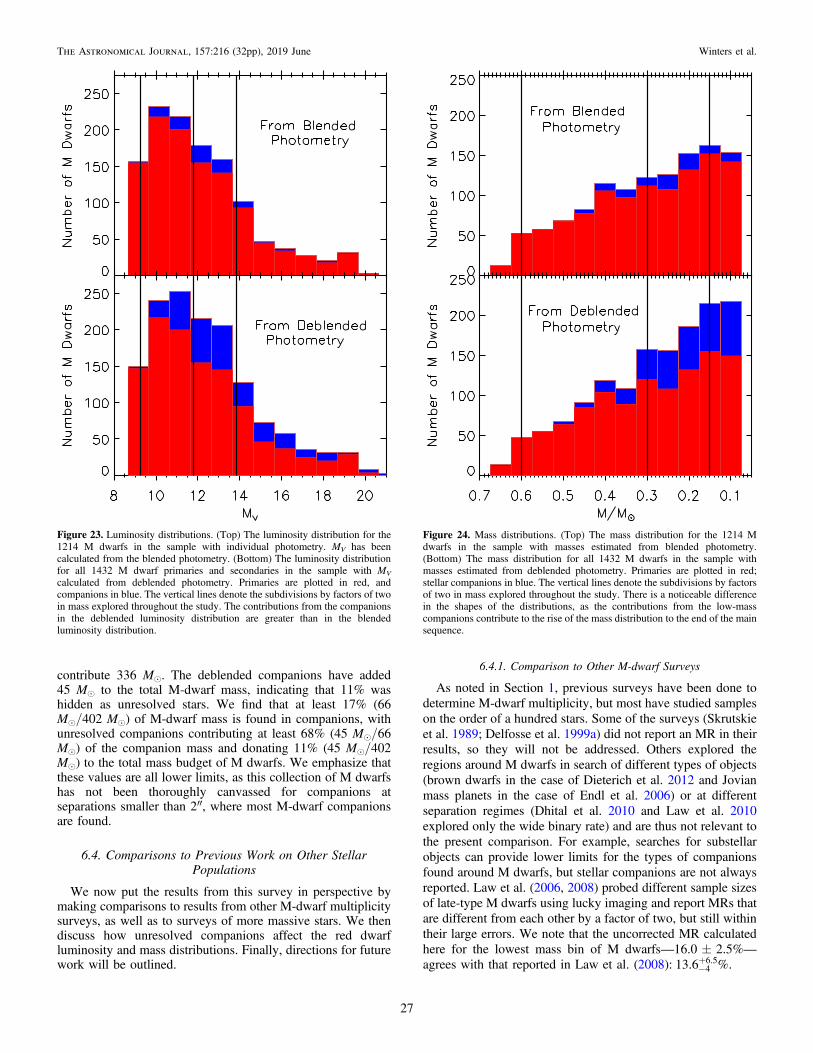
contribute 336 Me. The deblended companions have added45 Me to the total M-dwarf mass, indicating that 11% washidden as unresolved stars. We find that at least 17% (66Me/402 Me) of M-dwarf mass is found in companions, withunresolved companions contributing at least 68% (45 Me/66Me) of the companion mass and donating 11% (45 Me/402Me) to the total mass budget of M dwarfs. We emphasize thatthese values are all lower limits, as this collection of M dwarfshas not been thoroughly canvassed for companions atseparations smaller than 2″, where most M-dwarf companionsare found.

6.4. Comparisons to Previous Work on Other StellarPopulations

We now put the results from this survey in perspective bymaking comparisons to results from other M-dwarf multiplicitysurveys, as well as to surveys of more massive stars. We thendiscuss how unresolved companions affect the red dwarfluminosity and mass distributions. Finally, directions for futurework will be outlined.

6.4.1. Comparison to Other M-dwarf Surveys

As noted in Section 1, previous surveys have been done todetermine M-dwarf multiplicity, but most have studied sampleson the order of a hundred stars. Some of the surveys (Skrutskieet al. 1989; Delfosse et al. 1999a) did not report an MR in theirresults, so they will not be addressed. Others explored theregions around M dwarfs in search of different types of objects(brown dwarfs in the case of Dieterich et al. 2012 and Jovianmass planets in the case of Endl et al. 2006) or at differentseparation regimes (Dhital et al. 2010 and Law et al. 2010explored only the wide binary rate) and are thus not relevant tothe present comparison. For example, searches for substellarobjects can provide lower limits for the types of companionsfound around M dwarfs, but stellar companions are not alwaysreported. Law et al. (2006, 2008) probed different sample sizesof late-type M dwarfs using lucky imaging and report MRs thatare different from each other by a factor of two, but still withintheir large errors. We note that the uncorrected MR calculatedhere for the lowest mass bin of M dwarfs—16.0±2.5%—

agrees with that reported in Law et al. (2008): 13.6 %4

6.5

-+ .

Figure 23. Luminosity distributions. (Top) The luminosity distribution for the1214 M dwarfs in the sample with individual photometry. MV has beencalculated from the blended photometry. (Bottom) The luminosity distributionfor all 1432 M dwarf primaries and secondaries in the sample with MV

calculated from deblended photometry. Primaries are plotted in red, andcompanions in blue. The vertical lines denote the subdivisions by factors of twoin mass explored throughout the study. The contributions from the companionsin the deblended luminosity distribution are greater than in the blendedluminosity distribution.

Figure 24. Mass distributions. (Top) The mass distribution for the 1214 Mdwarfs in the sample with masses estimated from blended photometry.(Bottom) The mass distribution for all 1432 M dwarfs in the sample withmasses estimated from deblended photometry. Primaries are plotted in red;stellar companions in blue. The vertical lines denote the subdivisions by factorsof two in mass explored throughout the study. There is a noticeable differencein the shapes of the distributions, as the contributions from the low-masscompanions contribute to the rise of the mass distribution to the end of the mainsequence.

27


A number of the other samples studied for M-dwarfmultiplicity determination were volume-limited. Henry &McCarthy (1990) searched the 5 pc sample of M dwarfs, whileHenry (1991) and Simons et al. (1996) extended the volumesearched to 8 pc. Fischer & Marcy (1992) searched a variedsample of M dwarfs within 20 pc. The samples of Bergforset al. (2010), Janson et al. (2012), and Janson et al. (2014a)were all within 52 pc, but most distances were photometricparallaxes.

We find that our MR result agrees with most of the morerecent surveys. Bergfors et al. (2010), Janson et al. (2012), andJanson et al. (2014a) report MRs of 32%, 27%, and 21%–27%,respectively. Our results also agree with the earlier studies ofHenry & McCarthy (1990) and Henry (1991) (34% and 20%)

within the errors, but are smaller than the studies of Fischer &Marcy (1992) and Simons et al. (1996) (42% and 40%). It islikely that some of the earlier studies simply did not haveenough targets from which to calculate accurate results withlow statistical errors.

The only other sizeable survey that was volume-limited andhad trigonometric parallaxes available was that of Ward-Duonget al. (2015); however, their sample included late K dwarfs anddid not include any late-M dwarfs. We find a slightly largerMR than the 23.5±3.2% of Ward-Duong et al. (2015),although results agree within the errors. Examination of thesample studied here reveals an additional 308 M dwarfs withparallaxes from sources other than van Leeuwen (2007) thatplace them within 15 pc, 247 of which are within the color-limits of their sample (3.65<(V− K )6.8).21

Because all of the targets in our multiplicity sample haveaccurate trigonometric parallaxes, the study presented here hasa number of advantages over studies conducted by others. Allof the targets considered were reliably known to be within25 pc. Because we measured VRI photometry for almost alltargets lacking it, we were able to use a homogeneous set ofdata on the same photometric system, combined with theexisting parallaxes, to calculate MV and thus, estimate masses.Most other surveys were forced to use less accurate types ofdistances to draw conclusions from their data. We were alsoable to calculate projected separations that were more accuratethan those of others, as our sample has trigonometric distances.Finally, our survey was comprehensive in two search regimes,while it was also able to infer the presence of candidatecompanions using other methods.

6.4.2. Comparison to More Massive Stars

Listed in Table 15 are the multiplicity statistics for stars ofother main-sequence spectral types, along with the percentagesof all stars by that spectral type. While brown dwarfs are notmain-sequence objects, they have been included for compar-ison. The percentage of stars that they comprise has beenpurposely left blank, as they are not stars, and in fact, the sizeof the brown dwarf population is not well constrained.

While the MR decreases as a function of primary mass, it isevident that the number of stars increases with decreasing mass.Massive stars of types OBA are the rarest, accounting for fewerthan 1% of all stars (Binney & Merrifield 1998), while solar-type FGK stars make up ∼21% of all stars (Binney &Merrifield 1998). The M dwarfs make up 75% of all stars; thus,

their multiplicity statistics have the largest impact. The K dwarfMR is the most uncertain, with no comprehensive multiplicitysearch having yet been done for that spectral type, althoughefforts to remedy this are currently underway by members ofthe RECONS group. The thorough study presented hereprovides an anchor for the statistics at the low end of thestellar main sequence, enabling a complete picture of stellarmultiplicity.Figure 25 indicates the MRs for dwarf stars, with values

taken from the literature for the more massive main-sequencestars. The clear decrease in multiplicity with decreasingprimary mass is evident.From this comprehensive picture of stellar multiplicity, we

can determine the MR of all star systems. Consider one millionstars. Table 16 duplicates the percentages of stars for eachmain-sequence spectral type and the MR for each of thosespectral types from Table 15. In addition, however, is listed thenumber of stars per one million that each spectral type wouldcontribute and how many of those would be multiple. The extrathree percent of stars not shown in the second column aremade up of giants, supergiants, and white dwarfs

Figure 25. Multiplicity rate as a function of spectral type. Shown is the MR fordwarf stars, with the rates for M dwarfs presented here in red. Open red pointsare the uncorrected MRs for the three mass bins explored throughout this paper,while the solid point is the total corrected MR for all M dwarfs. Values for starsmore massive than M dwarfs are taken from the literature, as listed in Table 15.The open green and orange points are the blue and red subsamples fromRaghavan et al. (2010), while the solid yellow point is the average reported inthat paper. The arrows indicate the MRs that are likely lower limits. We do notinclude the L dwarfs here. Clearly, the MR is a function of decreasing mass.

Table 15

Multiplicity of Main-sequence Stars

Spectral % of References Mult. Comp ReferencesType Stars Rate Rate

O <0.1 2 >80 130 5, 3B 0.1 2 >70 100 6, 3A 0.6 2 >70 100 6, 3F 3.3 2 50±4 75 6G 7.8 2 46±2 75 6K 10.2 2 41±3 56 6M 75.0 4 26.8±1.4 32.4±1.4 1L, T L 22 22 3

Note.The columns indicate the spectral type of object, the percentage of starsthat each spectral type comprises, along with the reference. Next, themultiplicity rate, the companion rate, and the reference are listed.References.(1) This work; (2) Binney & Merrifield (1998); (3) Duchêne &Kraus (2013); (4) Henry et al. (2006); (5) Mason et al. (2009); (6) Raghavanet al. (2010).

21 This red limit has been estimated from the color–color diagram in Figure 1in their paper, as it is not specified.

28


(Binney & Merrifield 1998). Based on the numbers presented,we can conclude that the MR of all main-sequence star systemsis 31±0.05%, and that therefore most stellar systems aresingle.

7. Conclusions

7.1. Summary of Results

1. We report 20 new and 56 suspected companions to Mdwarfs within 25 pc.

2. We find a corrected MR of 26.8±1.4% and a correctedCR of 32.4±1.4% for M dwarfs.

3. We find that M dwarfs have MRs and CRs of20.2±1.2% and 23.9±1.4% at projected linearseparations <50 au.

4. We find the uncorrected MR of the three mass subsets(0.30–0.60 M/Me, 0.15–0.30 M/Me, and 0.075–0.15M/Me) to be 28.2±2.1%, 21.4±2.0%, and16.0± 2.5%.

5. We find a uniformity in the mass ratio distribution, withno apparent preference in companion mass for the nearbyM dwarfs.

6. The distribution of the projected separations of thecompanions peaks at 4–20 au for M dwarfs, i.e., the scaleof the gas giants in our solar system.

7. A weak trend of decreasing projected separation withprimary mass was found.

8. A possible relation between multiplicity and tangentialvelocity was found, indicating that older, faster movingM dwarfs tend to have fewer companions at smallerseparations as a population than their youngercounterparts.

9. We find that at least 17% of M dwarf mass is contained incompanions, with 11% of the total mass budget made upof “hidden” stellar companions.

10. Finally, we demonstrate that the mass distribution of ourvolume-limited sample rises to the end of the stellar mainsequence.

7.2. What Is Yet to Come

While the multiplicity survey presented here was compre-hensive for stellar companions to M dwarfs with separations2″–300″, much work remains to be done. Currently underwayare Robo-AO, high-resolution speckle imaging, and radialvelocity studies to probe within 2″ of these nearby M dwarfs inorder to complete our understanding of M-dwarf multiplicity atall separation regimes. The results from these ongoing surveys

will provide the separation and delta-magnitude measurementsneeded for a more thorough understanding of the characteristicsof these multiple systems, e.g., the mass ratio and separationdistributions. In addition, the radial velocities being measuredprovide the third velocity component needed to calculateprecise UVW space motions. These space motions will allowfurther exploration of the possible trend of stellar multiplicitywith tangential velocity.Gaia will have five years or more of exquisite astrometric

measurements that will enable the detection of binaries. Anyastrometric binary orbits should provide inclinations, and thusthe dynamical masses of each component when combined withground-based spectroscopic orbits. In addition, Gaia shouldreveal many of the very low-mass stars that have escapeddetection to date, providing a more complete picture of thenearby M-dwarf population that we will study in the future.

We thank the anonymous referee for a rigorous review thatgreatly improved the manuscript. J.G.W. is especially gratefulto Jonathan Irwin, Willie Torres, and Eric Mamajek forilluminating and clarifying discussions and suggestions, and toDouglas Gies, Harold McAlister, Russel White, SebastiénLépine, and David Charbonneau for constructive comments.We thank Brian Mason for access to the Washington DoubleStar Catalog, a copy of which is housed at Georgia StateUniversity. J.G.W. extends a heartfelt thanks to David Fanningfor the availability of his IDL Coyote Graphics System.We thank the members of the SMARTS Consortium, who

have enabled the operations of the small telescopes at CTIOsince 2003, as well as observers and observer support at CTIO,specifically Arturo Gomez, Mauricio Rojas, Hernan Tirado,Joselino Vasquez, Alberto Miranda, and Edgardo Cosgrove.We are indebted to the support staff and astronomers at LowellObservatory for their assistance, particularly Len Bright, LarryWasserman, Brian Skiff, and Ted Dunham.Data products from the Two Micron All Sky Survey, which

is a joint project of the University of Massachusetts and theInfrared Processing and Analysis Center/California Institute ofTechnology, funded by the National Aeronautics and SpaceAdministration (NASA) and the NSF have been usedextensively, as have the SIMBAD database and the Aladinand Vizier interfaces, operated at CDS, Strasbourg, France.This work has made ample use of the Smithsonian Astro-physical Observatory/NASA Astrophysics Data System. Thiswork has made use of data from the European SpaceAgency (ESA) mission Gaia (https://www.cosmos.esa.int/gaia), processed by the Gaia Data Processing and AnalysisConsortium (DPAC,https://www.cosmos.esa.int/web/gaia/dpac/consortium). Funding for the DPAC has been providedby national institutions, in particular the institutions participat-ing in the Gaia Multilateral Agreement.This work was made possible by National Science Founda-

tion (NSF) grants 09-08402, 0507711, 1109445, and 141206,Sigma Xi Grants-In-Aid-of-Research, the generous budgetallotment of Georgia State University that made possible accessto the SMARTS telescopes at CTIO and Lowell, and theGeorgia State University Dissertation grant. J.G.W. wassupported by a grant from the John Templeton Foundationfor a portion of the time that it took to finalize these results. Theopinions expressed here are those of the authors and do notnecessarily reflect the views of the John TempletonFoundation.

Table 16

Multiplicity Example

Spectral % of # of Mult. # Mult.Type Stars Stars Rate

O 0.003 30 80 24B 0.1 1,000 70 700A 0.6 6,000 70 4,200F 3.3 33,000 50 16,500G 7.8 78,000 46 35,880K 10.2 102,000 41 41,820M 75.0 750,000 26.8 201,000

97.0 970,030 31 300,124

29


Software:IRAF (Tody 1986, 1993), SExtractor (Bertin &Arnouts 1996), PSFEx (Bertin 2011).

ORCID iDs

Jennifer G. Winters https://orcid.org/0000-0001-6031-9513Wei-Chun Jao https://orcid.org/0000-0003-0193-2187John P. Subasavage https://orcid.org/0000-0001-5912-6191Adric R. Riedel https://orcid.org/0000-0003-1645-8596Michele L. Silverstein https://orcid.org/0000-0003-2565-7909Matthew J. Payne https://orcid.org/0000-0001-5133-6303

References

Allen, P. R., Koerner, D. W., McElwain, M. W., Cruz, K. L., & Reid, I. N.2007, AJ, 133, 971

Allen, P. R., & Reid, I. N. 2008, AJ, 135, 2024Al-Shukri, A. M., McAlister, H. A., Hartkopf, W. I., Hutter, D. J., &

Franz, O. G. 1996, AJ, 111, 393Andrei, A. H., Smart, R. L., Penna, J. L., et al. 2011, AJ, 141, 54Anglada-Escudé, G., Boss, A. P., Weinberger, A. J., et al. 2012, ApJ, 746, 37Balega, I. I., Balega, Y. Y., Gasanova, L. T., et al. 2013, AstBu, 68, 53Balega, I. I., Balega, Y. Y., Maksimov, A. F., et al. 2007, AstBu, 62, 339Barbieri, C., De Marchi, G., Nota, A., et al. 1996, A&A, 315, 418Bartlett, J. L., Lurie, J. C., Riedel, A., et al. 2017, AJ, 154, 151Benedict, G. F., McArthur, B. E., Franz, O. G., Wasserman, L. H., &

Henry, T. J. 2000, AJ, 120, 1106Benedict, G. F., McArthur, B., Chappell, D. W., et al. 1999, AJ, 118, 1086Benedict, G. F., McArthur, B. E., Franz, O. G., et al. 2001, AJ, 121, 1607Benedict, G. F., McArthur, B. E., Forveille, T., et al. 2002, ApJL, 581, L115Benedict, G. F., Henry, T. J., Franz, O. G., et al. 2016, AJ, 152, 141Bergfors, C., Brandner, W., Janson, M., et al. 2010, A&A, 520, A54Bertin, E. 2011, in ASP Conf. Ser. 442, Astronomical Data Analysis Software

and Systems XX, ed. I. N. Evans et al. (San Francisco, CA: ASP), 435Bertin, E., & Arnouts, S. 1996, A&AS, 117, 393Bessel, M. S. 1990, A&AS, 83, 357Bessell, M. S. 1991, AJ, 101, 662Bessell, M. S., & Weis, E. W. 1987, PASP, 99, 642Beuzit, J.-L., Ségransan, D., Forveille, T., et al. 2004, A&A, 425, 997Bidelman, W. P. 1985, ApJS, 59, 197Biller, B. A., & Close, L. M. 2007, ApJL, 669, L41Biller, B. A., Kasper, M., Close, L. M., Brandner, W., & Kellner, S. 2006,

ApJL, 641, L141Binney, J., & Merrifield, M. 1998, Galactic Astronomy (Princeton, NJ:

Princeton Univ. Press)Blake, C. H., Charbonneau, D., White, R. J., et al. 2008, ApJL, 678, L125Bonfils, X., Delfosse, X., Udry, S., et al. 2013, A&A, 549, A109Bonnefoy, M., Chauvin, G., Dumas, C., et al. 2009, A&A, 506, 799Bowler, B. P., Liu, M. C., Shkolnik, E. L., & Tamura, M. 2015, ApJS, 216, 7Burningham, B., Pinfield, D. J., Leggett, S. K., et al. 2009, MNRAS, 395, 1237Chanamé, J., & Gould, A. 2004, ApJ, 601, 289Cortes-Contreras, M., Caballero, J. A., & Montes, D. 2014, Obs, 134, 348Costa, E., Méndez, R. A., Jao, W.-C., et al. 2005, AJ, 130, 337Costa, E., Méndez, R. A., Jao, W.-C., et al. 2006, AJ, 132, 1234Cvetković, Z., Pavlović, R., & Boeva, S. 2015, AJ, 149, 150Daemgen, S., Siegler, N., Reid, I. N., & Close, L. M. 2007, ApJ, 654, 558Dahn, C. C., Harrington, R. S., Kallarakal, V. V., et al. 1988, AJ, 95, 237Dahn, C. C., Harris, H. C., Vrba, F. J., et al. 2002, AJ, 124, 1170Davison, C. L., White, R. J., Jao, W.-C., et al. 2014, AJ, 147, 26Davison, C. L., White, R. J., Henry, T. J., et al. 2015, AJ, 149, 106Dawson, P. C., & De Robertis, M. M. 2005, PASP, 117, 1Deacon, N. R., & Hambly, N. C. 2001, A&A, 380, 148Deacon, N. R., Hambly, N. C., & Cooke, J. A. 2005a, A&A, 435, 363Deacon, N. R., Hambly, N. C., Henry, T. J., et al. 2005b, AJ, 129, 409Delfosse, X., Forveille, T., Beuzit, J.-L., et al. 1999a, A&A, 344, 897Delfosse, X., Forveille, T., Perrier, C., & Mayor, M. 1998, A&A, 331, 581Delfosse, X., Forveille, T., Udry, S., et al. 1999b, A&A, 350, L39Dhital, S., West, A. A., Stassun, K. G., & Bochanski, J. J. 2010, AJ, 139, 2566Díaz, R. F., González, J. F., Cincunegui, C., & Mauas, P. J. D. 2007, A&A,

474, 345Dieterich, S. B., Henry, T. J., Golimowski, D. A., Krist, J. E., & Tanner, A. M.

2012, AJ, 144, 64

Dieterich, S. B., Henry, T. J., Jao, W.-C., et al. 2014, AJ, 147, 94Docobo, J. A., Tamazian, V. S., Balega, Y. Y., & Melikian, N. D. 2006, AJ,

132, 994Docobo, J. A., Tamazian, V. S., Balega, Y. Y., & Melikian, N. D. 2010, AJ,

140, 1078Doyle, J. G., & Butler, C. J. 1990, A&A, 235, 335Duchêne, G., & Kraus, A. 2013, ARA&A, 51, 269Dupuy, T. J., & Liu, M. C. 2012, ApJS, 201, 19Duquennoy, A., & Mayor, M. 1988, A&A, 200, 135Endl, M., Cochran, W. D., Kürster, M., et al. 2006, ApJ, 649, 436Fabricius, C., & Makarov, V. V. 2000, A&AS, 144, 45Faherty, J. K., Burgasser, A. J., Walter, F. M., et al. 2012, ApJ, 752, 56Falin, J. L., & Mignard, F. 1999, A&AS, 135, 231Femenía, B., Rebolo, R., Pérez-Prieto, J. A., et al. 2011, MNRAS, 413, 1524Fischer, D. A., & Marcy, G. W. 1992, ApJ, 396, 178Forveille, T., Beuzit, J.-L., Delorme, P., et al. 2005, A&A, 435, L5Frankowski, A., Jancart, S., & Jorissen, A. 2007, A&A, 464, 377Freed, M., Close, L. M., & Siegler, N. 2003, ApJ, 584, 453Fu, H.-H., Hartkopf, W. I., Mason, B. D., et al. 1997, AJ, 114, 1623Gaia Collaboration, Brown, A. G. A., Vallenari, A., et al. 2018, A&A, 616, A1Gaia Collaboration, Prusti, T., de Bruijne, J. H. J., et al. 2016, A&A, 595, A1Gatewood, G. 2008, AJ, 136, 452Gatewood, G., & Coban, L. 2009, AJ, 137, 402Gatewood, G., Coban, L., & Han, I. 2003, AJ, 125, 1530Gatewood, G., de Jonge, K. J., & Stephenson, B. 1993, PASP, 105, 1101Gershberg, R. E., Katsova, M. M., Lovkaya, M. N., Terebizh, A. V., &

Shakhovskaya, N. I. 1999, A&AS, 139, 555Gianninas, A., Bergeron, P., & Ruiz, M. T. 2011, ApJ, 743, 138Gizis, J. E. 1997, AJ, 113, 806Gizis, J. E. 1998, AJ, 115, 2053Gizis, J. E., Reid, I. N., & Hawley, S. L. 2002, AJ, 123, 3356Golimowski, D. A., Leggett, S. K., Marley, M. S., et al. 2004, AJ, 127, 3516Gould, A., & Chanamé, J. 2004, ApJS, 150, 455Graham, J. A. 1982, PASP, 94, 244Gray, R. O., Corbally, C. J., Garrison, R. F., McFadden, M. T., &

Robinson, P. E. 2003, AJ, 126, 2048Harlow, J. J. B. 1996, AJ, 112, 2222Harrington, R. S., & Dahn, C. C. 1980, AJ, 85, 454Harrington, R. S., Kallarakal, V. V., Christy, J. W., et al. 1985, AJ, 90, 123Harrington, R. S., Dahn, C. C., Kallarakal, V. V., et al. 1993, AJ, 105, 1571Hartkopf, W. I., Tokovinin, A., & Mason, B. D. 2012, AJ, 143, 42Hawley, S. L., Gizis, J. E., & Reid, I. N. 1996, AJ, 112, 2799Heintz, W. D. 1976, MNRAS, 175, 533Heintz, W. D. 1985, ApJS, 58, 439Heintz, W. D. 1986, AJ, 92, 446Heintz, W. D. 1987, ApJS, 65, 161Heintz, W. D. 1990, ApJS, 74, 275Heintz, W. D. 1991, AJ, 101, 1071Heintz, W. D. 1992, ApJS, 83, 351Heintz, W. D. 1993, AJ, 105, 1188Heintz, W. D. 1994, AJ, 108, 2338Hełminiak, K. G., Konacki, M., Kulkarni, S. R., & Eisner, J. 2009, MNRAS,

400, 406Henry, T. J. 1991, PhD thesis, Arizona Univ., Tucson.Henry, T. J., Franz, O. G., Wasserman, L. H., et al. 1999, ApJ, 512, 864Henry, T. J., Ianna, P. A., Kirkpatrick, J. D., & Jahreiss, H. 1997, AJ, 114, 388Henry, T. J., Jao, W.-C., Subasavage, J. P., et al. 2006, AJ, 132, 2360Henry, T. J., & McCarthy, D. W., Jr. 1990, ApJ, 350, 334Henry, T. J., Subasavage, J. P., Brown, M. A., et al. 2004, AJ, 128, 2460Henry, T. J., Jao, W.-C., Winters, J. G., et al. 2018, AJ, 155, 265Herbig, G. H., & Moorhead, J. M. 1965, ApJ, 141, 649Hershey, J. L., & Taff, L. G. 1998, AJ, 116, 1440Høg, E., Fabricius, C., Makarov, V. V., et al. 2000, A&A, 355, L27Holman, M. J., & Wiegert, P. A. 1999, AJ, 117, 621Horch, E. P., Bahi, L. A. P., Gaulin, J. R., et al. 2012, AJ, 143, 10Horch, E. P., Casetti-Dinescu, D. I., Camarata, M. A., et al. 2017, AJ, 153, 212Horch, E. P., Falta, D., Anderson, L. M., et al. 2010, AJ, 139, 205Horch, E. P., Gomez, S. C., Sherry, W. H., et al. 2011a, AJ, 141, 45Horch, E. P., Robinson, S. E., Meyer, R. D., et al. 2002, AJ, 123, 3442Horch, E. P., van Altena, W. F., Demarque, P., et al. 2015a, AJ, 149, 151Horch, E. P., van Altena, W. F., Howell, S. B., Sherry, W. H., & Ciardi, D. R.

2011b, AJ, 141, 180Horch, E. P., van Belle, G. T., Davidson, J. W., Jr., et al. 2015b, AJ, 150, 151Horch, E. P., Veillette, D. R., Baena Gallé, R., et al. 2009, AJ, 137, 5057Hosey, A. D., Henry, T. J., Jao, W.-C., et al. 2015, AJ, 150, 6Houdebine, E. R. 2010, MNRAS, 407, 1657

30


Howell, S. B. 2000, Handbook of CCD Astronomy (Cambridge: CambridgeUniv. Press)

Howell, S. B. 2012, PASP, 124, 263Ianna, P. A., Patterson, R. J., & Swain, M. A. 1996, AJ, 111, 492Ireland, M. J., Kraus, A., Martinache, F., Lloyd, J. P., & Tuthill, P. G. 2008,

ApJ, 678, 463Jahreiß, H., Meusinger, H., Scholz, R.-D., & Stecklum, B. 2008, A&A,

484, 575Jancart, S., Jorissen, A., Babusiaux, C., & Pourbaix, D. 2005, A&A, 442, 365Janson, M., Bergfors, C., Brandner, W., et al. 2014a, ApJ, 789, 102Janson, M., Bergfors, C., Brandner, W., et al. 2014b, ApJS, 214, 17Janson, M., Hormuth, F., Bergfors, C., et al. 2012, ApJ, 754, 44Jao, W.-C., Henry, T. J., Beaulieu, T. D., & Subasavage, J. P. 2008, AJ,

136, 840Jao, W.-C., Henry, T. J., Subasavage, J. P., et al. 2003, AJ, 125, 332Jao, W.-C., Henry, T. J., Subasavage, J. P., et al. 2005, AJ, 129, 1954Jao, W.-C., Henry, T. J., Subasavage, J. P., et al. 2014, AJ, 147, 21Jao, W.-C., Henry, T. J., Subasavage, J. P., et al. 2011, AJ, 141, 117Jao, W.-C., Henry, T. J., Winters, J. G., et al. 2017, AJ, 154, 191Jao, W.-C., Mason, B. D., Hartkopf, W. I., Henry, T. J., & Ramos, S. N. 2009,

AJ, 137, 3800Jenkins, J. S., Ramsey, L. W., Jones, H. R. A., et al. 2009, ApJ, 704, 975Jódar, E., Pérez-Garrido, A., Díaz-Sánchez, A., et al. 2013, MNRAS, 429, 859Khovritchev, M. Y., Izmailov, I. S., & Khrutskaya, E. V. 2013, MNRAS,

435, 1083Kirkpatrick, J. D., & McCarthy, D. W., Jr. 1994, AJ, 107, 333Kleinman, S. J., Harris, H. C., Eisenstein, D. J., et al. 2004, ApJ, 607, 426Koen, C., Kilkenny, D., van Wyk, F., Cooper, D., & Marang, F. 2002,

MNRAS, 334, 20Koen, C., Kilkenny, D., van Wyk, F., & Marang, F. 2010, MNRAS, 403, 1949Köhler, R., Ratzka, T., & Leinert, C. 2012, A&A, 541, A29Kraus, A. L., Ireland, M. J., Huber, D., Mann, A. W., & Dupuy, T. J. 2016, AJ,

152, 8Kürster, M., Endl, M., & Reffert, S. 2008, A&A, 483, 869Kürster, M., Zechmeister, M., Endl, M., & Meyer, E. 2009, Msngr, 136, 39Lampens, P., Strigachev, A., & Duval, D. 2007, A&A, 464, 641Landolt, A. U. 1992, AJ, 104, 372Landolt, A. U. 2007, AJ, 133, 2502Landolt, A. U. 2009, AJ, 137, 4186Landolt, A. U. 2013, AJ, 146, 131Law, N. M., Dhital, S., Kraus, A., Stassun, K. G., & West, A. A. 2010, ApJ,

720, 1727Law, N. M., Hodgkin, S. T., & Mackay, C. D. 2006, MNRAS, 368, 1917Law, N. M., Hodgkin, S. T., & Mackay, C. D. 2008, MNRAS, 384, 150Leinert, C., Henry, T., Glindemann, A., & McCarthy, D. W., Jr. 1997, A&A,

325, 159Leinert, C., Weitzel, N., Richichi, A., Eckart, A., & Tacconi-Garman, L. E.

1994, A&A, 291, L47Lèpine, S., & Shara, M. M. 2005, AJ, 129, 1483Lèpine, S., Thorstensen, J. R., Shara, M. M., & Rich, R. M. 2009, AJ,

137, 4109Lindegren, L., Mignard, F., Söderhjelm, S., et al. 1997, A&A, 323, L53Lurie, J. C., Henry, T. J., Jao, W.-C., et al. 2014, AJ, 148, 91Luyten, W. J. 1979a, LHS Catalogue (2nd ed.; Minneapolis, MN: Univ.

Minnesota)Luyten, W. J. 1979b, NLTT Catalogue, Vol. I and Vol. II (Minneapolis, MN:

Univ. Minnesota)Luyten, W. J. 1980a, NLTT Catalogue, Vol. III (Minneapolis, MN: Univ.

Minnesota)Luyten, W. J. 1980b, NLTT Catalogue, Vol. IV (Minneapolis, MN: Univ.

Minnesota)Malo, L., Artigau, É., Doyon, R., et al. 2014, ApJ, 788, 81Mamajek, E. E. 2016, in IAU Symp. 314, Young Stars & Planets Near the

Sun, ed. J. H. Kastner, B. Stelzer, & S. A. Metchev, 21Mamajek, E. E., Bartlett, J. L., Seifahrt, A., et al. 2013, AJ, 146, 154Marcy, G. W., & Benitz, K. J. 1989, ApJ, 344, 441Marcy, G. W., Lindsay, V., & Wilson, K. 1987, PASP, 99, 490Martin, C., & Mignard, F. 1998, A&A, 330, 585Martín, E. L., Koresko, C. D., Kulkarni, S. R., Lane, B. F., &

Wizinowich, P. L. 2000, ApJL, 529, L37Martinache, F., Lloyd, J. P., Ireland, M. J., Yamada, R. S., & Tuthill, P. G.

2007, ApJ, 661, 496Martinache, F., Rojas-Ayala, B., Ireland, M. J., Lloyd, J. P., & Tuthill, P. G.

2009, ApJ, 695, 1183Mason, B. D., Hartkopf, W. I., Gies, D. R., Henry, T. J., & Helsel, J. W. 2009,

AJ, 137, 3358

Mason, B. D., Hartkopf, W. I., Miles, K. N., et al. 2018, AJ, 155, 215McAlister, H. A., Hartkopf, W. I., Hutter, D. J., & Franz, O. G. 1987, AJ,

93, 688McLean, I. S., McGovern, M. R., Burgasser, A. J., et al. 2003, ApJ, 596, 561Meyer, R. D., Horch, E. P., Ninkov, Z., van Altena, W. F., & Rothkopf, C. A.

2006, PASP, 118, 162Monet, D. G., Levine, S. E., Canzian, B., et al. 2003, AJ, 125, 984Montagnier, G., Ségransan, D., Beuzit, J.-L., et al. 2006, A&A, 460, L19Montet, B. T., Crepp, J. R., Johnson, J. A., Howard, A. W., & Marcy, G. W.

2014, ApJ, 781, 28Morgan, D. H. 1995, in ASP Conf. Ser. 84, IAU Coll. 148: The Future

Utilisation of Schmidt Telescopes, ed. J. Chapman et al. (San Francisco,CA: ASP), 137

Nidever, D. L., Marcy, G. W., Butler, R. P., Fischer, D. A., & Vogt, S. S. 2002,ApJS, 141, 503

Perryman, M. A. C., Lindegren, L., Kovalevsky, J., et al. 1997, A&A, 323, L49Platais, I., Pourbaix, D., Jorissen, A., et al. 2003, A&A, 397, 997Pokorny, R. S., Jones, H. R. A., Hambly, N. C., & Pinfield, D. J. 2004, A&A,

421, 763Pourbaix, D., Platais, I., Detournay, S., et al. 2003, A&A, 399, 1167Pourbaix, D., Tokovinin, A. A., Batten, A. H., et al. 2004, A&A, 424, 727Poveda, A., Herrera, M. A., Allen, C., Cordero, G., & Lavalley, C. 1994,

RMxAA, 28, 43Pravdo, S. H., & Shaklan, S. B. 2009, ApJ, 700, 623Pravdo, S. H., Shaklan, S. B., Henry, T., & Benedict, G. F. 2004, ApJ,

617, 1323Pravdo, S. H., Shaklan, S. B., Wiktorowicz, S. J., et al. 2006, ApJ, 649, 389Raghavan, D., McAlister, H. A., Henry, T. J., et al. 2010, ApJS, 190, 1Reid, I. N., Cruz, K. L., Laurie, S. P., et al. 2003, AJ, 125, 354Reid, I. N., Gizis, J. E., Kirkpatrick, J. D., & Koerner, D. W. 2001, AJ,

121, 489Reid, I. N., Hawley, S. L., & Gizis, J. E. 1995, AJ, 110, 1838Reid, I. N., Kilkenny, D., & Cruz, K. L. 2002, AJ, 123, 2822Reiners, A., & Basri, G. 2010, ApJ, 710, 924Reiners, A., Joshi, N., & Goldman, B. 2012, AJ, 143, 93Riddle, R. K., Priser, J. B., & Strand, K. A. 1971, PUSNO, 20, 1Riedel, A. R., Blunt, S. C., Lambrides, E. L., et al. 2017, AJ, 153, 95Riedel, A. R., Finch, C. T., Henry, T. J., et al. 2014, AJ, 147, 85Riedel, A. R., Murphy, S. J., Henry, T. J., et al. 2011, AJ, 142, 104Riedel, A. R., Silverstein, M. L., Henry, T. J., et al. 2018, AJ, 156, 2Riedel, A. R., Subasavage, J. P., Finch, C. T., et al. 2010, AJ, 140, 897Salim, S., & Gould, A. 2003, ApJ, 582, 1011Schilbach, E., Röser, S., & Scholz, R.-D. 2009, A&A, 493, L27Schmidt, S. J., Cruz, K. L., Bongiorno, B. J., Liebert, J., & Reid, I. N. 2007,

AJ, 133, 2258Schneider, A., Melis, C., Song, I., & Zuckerman, B. 2011, ApJ, 743, 109Scholz, R.-D. 2010, A&A, 515, A92Ségransan, D., Delfosse, X., Forveille, T., et al. 2000, A&A, 364, 665Shakht, N. A. 1997, A&AT, 13, 327Shkolnik, E. L., Anglada-Escudé, G., Liu, M. C., et al. 2012, ApJ, 758, 56Shkolnik, E. L., Hebb, L., Liu, M. C., Reid, I. N., & Collier Cameron, A. 2010,

ApJ, 716, 1522Siegler, N., Close, L. M., Cruz, K. L., Martín, E. L., & Reid, I. N. 2005, ApJ,

621, 1023Simons, D. A., Henry, T. J., & Kirkpatrick, J. D. 1996, AJ, 112, 2238Skrutskie, M. F., Forrest, W. J., & Shure, M. 1989, AJ, 98, 1409Skrutskie, M. F., Cutri, R. M., Stiening, R., et al. 2006, AJ, 131, 1163Smart, R. L., Ioannidis, G., Jones, H. R. A., Bucciarelli, B., & Lattanzi, M. G.

2010, A&A, 514, A84Smart, R. L., Lattanzi, M. G., Jahreiß, H., Bucciarelli, B., & Massone, G. 2007,

A&A, 464, 787Snodgrass, C., & Carry, B. 2013, Msngr, 152, 14Söderhjelm, S. 1999, A&A, 341, 121Subasavage, J. P., Henry, T. J., Hambly, N. C., Brown, M. A., & Jao, W.-C.

2005a, AJ, 129, 413Subasavage, J. P., Henry, T. J., Hambly, N. C., et al. 2005b, AJ, 130, 1658Subasavage, J. P., Jao, W.-C., Henry, T. J., et al. 2009, AJ, 137, 4547Subasavage, J. P., Jr. 2007, PhD thesis, Georgia State Univ.Tamazian, V. S., Docobo, J. A., Melikian, N. D., & Karapetian, A. A. 2006,

PASP, 118, 814Tanner, A. M., Gelino, C. R., & Law, N. M. 2010, PASP, 122, 1195Teegarden, B. J., Pravdo, S. H., Hicks, M., et al. 2003, ApJL, 589, L51Teixeira, R., Ducourant, C., Chauvin, G., et al. 2009, A&A, 503, 281Tinney, C. G. 1996, MNRAS, 281, 644Tinney, C. G., Reid, I. N., Gizis, J., & Mould, J. R. 1995, AJ, 110, 3014Tody, D. 1986, Proc. SPIE, 627, 733

31


Tody, D. 1993, in ASP Conf. Ser. 52, Astronomical Data Analysis Softwareand Systems II, ed. R. J. Hanisch, R. J. V. Brissenden, & J. Barnes (SanFrancisco, CA: ASP), 173

Tokovinin, A., & Lépine, S. 2012, AJ, 144, 102Tokovinin, A. A. 1992, A&A, 256, 121van Altena, W. F., Lee, J. T., & Hoffleit, D. 1995, yCat, 1174, 0van Biesbroeck, G. 1974, ApJS, 28, 413van de Kamp, P. 1975, ARA&A, 13, 295van de Kamp, P., & Worth, M. D. 1972, AJ, 77, 762van Dessel, E., & Sinachopoulos, D. 1993, A&AS, 100, 517van Leeuwen, F. 2007, A&A, 474, 653von Braun, K., Boyajian, T. S., Kane, S. R., et al. 2011, ApJL, 729, L26Wahhaj, Z., Liu, M. C., Biller, B. A., et al. 2011, ApJ, 729, 139Wang, J., Fischer, D. A., Xie, J.-W., & Ciardi, D. R. 2014, ApJ, 791, 111Ward-Duong, K., Patience, J., De Rosa, R. J., et al. 2015, MNRAS, 449, 2618Weis, E. W. 1984, ApJS, 55, 289Weis, E. W. 1986, AJ, 91, 626Weis, E. W. 1987, AJ, 93, 451

Weis, E. W. 1988, Ap&SS, 142, 223Weis, E. W. 1991a, AJ, 102, 1795Weis, E. W. 1991b, AJ, 101, 1882Weis, E. W. 1993, AJ, 105, 1962Weis, E. W. 1994, AJ, 107, 1135Weis, E. W. 1996, AJ, 112, 2300Weis, E. W. 1999, AJ, 117, 3021Winn, J. N., & Fabrycky, D. C. 2015, ARA&A, 53, 409Winters, J. G., Henry, T. J., Jao, W.-C., et al. 2011, AJ, 141, 21Winters, J. G., Henry, T. J., Lurie, J. C., et al. 2015, AJ, 149, 5Winters, J. G., Irwin, J., Newton, E. R., et al. 2018, AJ, 155, 125Winters, J. G., Sevrinsky, R. A., Jao, W.-C., et al. 2017, AJ, 153, 14Woitas, J., Tamazian, V. S., Docobo, J. A., & Leinert, C. 2003, A&A, 406, 293Worley, C. E. 1961, PASP, 73, 167Worley, C. E. 1962, AJ, 67, 396Worley, C. E., & Mason, B. D. 1998, AJ, 116, 917Young, A., Sadjadi, S., & Harlan, E. 1987, ApJ, 314, 272Zechmeister, M., Kürster, M., & Endl, M. 2009, A&A, 505, 859

32


The Solar Neighborhood. XLV. The Stellar Multiplicity Rate ...

Documents

Transcript of The Solar Neighborhood. XLV. The Stellar Multiplicity Rate ...