The Slug Flow Problem in Oil Industry and Pi Level...

Chapter 0

The Slug Flow Problem in OilIndustry and Pi Level Control

Airam Sausen, Paulo Sausen and Mauricio de Campos

Additional information is available at the end of the chapter

http://dx.doi.org/10.5772/50711

1. Introduction

The slug is a multiphase flow pattern that occurs in pipelines which connect the wells inseabed to production platforms in the surface in oil industry. It is characterized by irregularflows and surges from the accumulation of gas and liquid in any cross-section of a pipeline. Inthis work will be addressed the riser slugging, that combined or initiated by terrain sluggingis the most serious case of instability in oil/water-dominated systems [5, 15, 21].

The cyclic behavior of the riser slugging, which is illustrated in Figure 1, can be dividedinto four phases: (i) Formation: gravity causes the liquid to accumulate in the low pointin pipeline-riser system and the gas and liquid velocity is low enough to enable for thisaccumulation; (ii) Production: the liquid blocks the gas flow and a continuous liquid slugis produced in the riser, as long as the hydrostatic head of the liquid in the riser increasesfaster than the pressure drop over the pipeline-riser system, the slug will continue to grow;(iii) Blowout: when the pressure drop over the riser overcomes the hydrostatic head of theliquid in the riser the slug will be pushed out of the system; (iv) liquid fall back: after themajority of the liquid and the gas has left the riser the velocity of the gas is no longer highenough to drag the liquid upwards, the liquid will start flowing back down the riser and theaccumulation of liquid starts over again [15].

The slug flow causes undesired consequences in the whole oil production such as: periodswithout liquid or gas production into the separator followed by very high liquid and gasrates when the liquid slug is being produced, emergency shutdown of the platform due tothe high level of liquid in the separators, floods, corrosion and damages to the equipments ofthe process, high costs with maintenance. One or all these problems cause significant lossesin oil industry. The main one has been of economic order, due to reduction in oil productioncapacity [6, 8, 16–20].

Currently, control strategies are considered as a promising solution to handle the slug flow [4,5, 7, 10, 15, 20]. An alternative to the implementation of control strategies is to make use ofa mathematical model that represents the dynamic of slug flow in pipeline-separator system.

©2012 Sausen et al., licensee InTech. This is an open access chapter distributed under the terms of theCreative Commons Attribution License (http://creativecommons.org/licenses/by/3.0),which permitsunrestricted use, distribution, and reproduction in any medium, provided the original work is properlycited.

Chapter 5

2 Will-be-set-by-IN-TECH

Figure 1. Illustration of a slug cycle.

In this chapter has been used the dynamic model for a pipeline-separator system under theslug flow, with 5 (five) Ordinary Differential Equations (ODEs) coupled, nonlinear, 6 (six)tuning parameters and more than 40 (forty) internal, geometric and transport equations [10,13], denominated Sausen’s model.

To carry out the simulation and implementation of control strategies in the Sausen’s model,first it is necessary to calculate its tuning parameters. For this procedure, are used datafrom a case study performed by [18] in the OLGA commercial multiphase simulator widelyused in the oil industry. Next it is important to check how the main variables of the modelchange their behavior considering a change in the model’s tuning parameters. This testing,called sensitivity analysis, is an important tool to the building of the mathematical models,moreover, it provides a better understanding of the dynamic behavior of the system, for laterimplementation of control strategies.

In this context, from the sensitivity analysis, the Sausen’s model has been an appropriateenvironment for application of the different feedback control strategies in the problem of theslug in oil industries through simulations. The model enables such strategies can be appliedin consequence the slug, that is in the oil or gas output valve separator, as well as in theircauses, in the top riser valve, or yet in the integrated system, in other words, in more than onevalve simultaneously.

Therefore, as part of control strategies that can be used to avoid or minimize the slug flow,this chapter presents the application of the error-squared level control strategy ProportionalIntegral (PI) in the methodology by bands [10], whose purpose damping of the load flow rateoscillatory that occur in production’s separators. This strategy is compared with the levelcontrols strategy PI conventional [1], widely used in industrial processes; and with the levelcontrol strategy PI also in the methodology by bands.

The remainder of this chapter is organized as following. Section 2 presents the equation of theSausen’s model for a pipeline-separator system. Section 3 shows the simulation results of theSausen’s model. Section 4 presents the control strategies used to avoid or minimize the slug

104 New Technologies in the Oil and Gas Industry

The Slug Flow Problem in Oil Industry and Pi Level Control 3

flow. Section 5 shows the simulation results and analysis of the control strategies applied theSausen’s model. And finally, in Section 6, are discussed the conclusions and future researchdirections.

2. The dynamic model

2.1. Introduction

This section presents a mathematical model for the pipeline-separator system, illustrated inFigure 2 with biphase flow (gas-liquid). The model is the result of coupling the simplifieddynamic model of Storkaas [15, 17, 20] with the model for a biphase horizontal cylindricalseparator [22]. The new model has been called of Sausen’s model.

The following are shown the modelling assumptions, the model equations, how thedistribution of liquid and gas inside the pipeline for the separator occurs. Finally, arepresented the simulation results for this model considering two settings for simulations: (i)the opening valve Z in top of the riser z = 20% (flow steady); and (ii) the opening valve Z intop of the riser z = 50% (slug flow).

Figure 2. Illustration of the pipeline-separator system with the slug formation.

2.2. Model assumption

The Sausen’s model assumptions are presented as follow.

A1: Liquid dynamics in the upstream feed section of the pipeline have been neglected, thatis, the liquid velocity in this section is constant.

A2: Follows from assumption A1 that the gas volume is constant in the upstream feed sectionpipeline and that the volume variations due to liquid level h1(t) at the low point areneglected.

A3: Only one dynamical state ML(t) for holdup liquid in the riser section. This state includesboth the liquid in the riser and at the low point section (with level h1(t)).

A4: Two dynamical states for holdup gas (MG1 and MG2(t)) occupying the volumes VG1and VG2(t), respectively. The gas volumes are related to each other by a pressure-flowrelationship at the low point.

105The Slug Flow Problem in Oil Industry and Pi Level Control


A5: Simplified valve equation for gas and liquid mixture leaving the system at the top of theriser.

A6: Stationary pressure balance over the riser (between pressures P1(t) and P2(t)).

A7: There is not chemical reaction between the fluids (gas-liquid) in pipeline.

A8: Each one of the fluid consists of a single component in the separator.

A9: The portion of liquid mixed with the gas in the entrance of the separator is neglected.

A10: Simplified valve equation for the gas and the liquid leaving the separator.

A11: The liquid is incompressible.

A12: The temperature is constant.

A13: The gas has ideal behavior.

2.3. Model equations

The Sausen’s model is composed of 5 (five) ODEs that are based on the mass conservationequations. The equations (1)-(3) represent the dynamics of the pipeline system and theequations (4)-(5) represent the dynamics of the separator:

ML(t) = mL,in −mL,out(t) (1)

MG1(t) = mG,in−mGint(t) (2)

MG2(t) = mG1(t)−mG,out(t) (3)

N(t) =

√r2

s − (rs − N(t))2

2H4ρL N(t) [3rs − 2N(t)][mL,out(t)−mLS,out(t)] (4)

PG1(t) ={ρLΦ[mG,out(t)−mGS,out(t)] + PG1(t) [mL,out(t)−mLS,out(t)]}

ρL[VS −VLS(t)](5)

where: ML(t) is the liquid mass at low point in the pipeline, (kg); MG1(t) is the gas mass in theupstream feed section of pipeline, (kg); MG2(t) is the gas mass at the top of the riser, (kg); N(t)is the liquid level in the separator, (m); PG1(t) is the gas pressure in the separator, (N/m2);and the ML(t), MG1(t), MG2(t), N(t), PG1(t) are their respective derivatives in relation totime; mL,in is the liquid mass flowrate that enters the upstream feed section of the pipeline,(kg/s); mG,in is the gas mass flowrate that enters in the upstream feed section of the pipeline,(kg/s); mL,out(t) is the liquid mass flowrate leaving through the valve at the top of the riserenters the separator, (kg/s); mG,out(t) is the gas mass flowrate leaving through the valve at thetop of the riser enters the separator, (kg/s); mGint(t) is the internal gas mass flowrate, (kg/s);mLS,out(t) is the liquid mass flowrate that leaves the separator through the valve Va1, (kg/s);mGS,out(t) is the gas mass flowrate that leaves the separator through the valve Va2, (kg/s); rsis the separator ray, (m); H4 is the separator length, (m); ρL is the liquid density, (kg/m3); VSis the separator volume, (m3); VLS(t) is the liquid volume in the separator, (m3); Φ = RT

MGis

a constant; R is the ideal gas constant (8314 JK.kmol ); T is the temperature, (K); MG is the gas

molecular weight, (kg/kmol).

The stationary pressure balance over the riser is assumed to be given by

P1(t)− P2(t) = gρ(t)H2 − ρLgh1(t)



where: P1(t) is the gas pressure in the upstream feed section of the pipeline, (N/m2); P2(t) isthe gas pressure at the top of the riser, (N/m2); g is the gravity (9.81m/s2); ρ(t) is the averagemixture density in the riser, (kg/m3); H2 is the riser height, (m); h1(t) is the liquid level at thedecline, (m).

A simplified valve equation is used to describe the flow through the Z valve at the top of theriser that is given by

mmix,out(t) = zK1

√ρT(t)(P2(t)− PG1(t)) (6)

where: z is the valve position (0− 100%); K1 is the valve constant and a tuning parameter;ρT(t) is the density upstream valve, (kg/m3); PG1(t) is the gas pressure into the separator,(N/m2). It is possible to observe that the coupling between the pipeline and the separatoroccurs through a pressure relationship, in other words, the gas pressure into the separatorPG1(t) is the pressure before the Z valve at the top of the riser, according to equation (6).

Considering the result that has been shown in equation (6), it is also possible to obtain theliquid mass flowrate given by

mL,out(t) = αmL (t)mmix,out(t)

and the gas mass flowrate given by

mG,out(t) = [1− αmL (t)]mmix,out(t)

that leave through the Z valve at the top of the riser, where αmL (t) is the liquid fraction

upstream valve.

The liquid mass flowrate that leaves the separator is represented by the Va1 valve equationgiven by

mLS,out(t) = zLK4

√ρL[PG1(t) + gρL N(t)− POL2] (7)

where: zL is the liquid valve opening (0 − 100%); K4 is the valve constant and a tuningparameter; POL2 is the downstream pressure after the Va1 valve, (N/m2).

The gas mass flowrate that leaves the separator is represented by the Va2 valve equation givenby

mGS,out(t) = zGK5

√ρG(t)[PG1(t)− PG2] (8)

where: zG is the gas valve position (0− 100%); K5 is the valve constant and a tuning parameter;ρG(t) is the gas density, (kg/m3); PG2 is the downstream pressure after the Va2 valve, (N/m2).

The boundary condition at the inlet (inflow mL,in and mG,in) can either be constant ordependent on the pressure. In this work they are constant and have been considereddisturbances of the process. The most critical section of the model is the phase distributionand phase velocities of the fluids in the pipeline-riser system. The gas velocity is based on anassumption of purely frictional pressure drop over the low point and the liquid distributionis based on an entrainment model. Finally, the internal, geometric and transport equations forthe pipeline system are found in [15, 17, 20].



2.4. Displacement of the gas flow

The displacement of gas in the pipeline system occurs through a relationship between the gasmass flow and the variation of the pressure inside the pipeline. The acceleration has beenneglected for the gas phase, so that it is the difference of the pressure that makes the fluidsoutflow pipeline above. Its equation is given by

ΔP(t) = P1(t)− [P2(t) + gρLαL(t)H2]

where: αL(t) is the average liquid fraction in riser.

It is considered that there are two situations in the riser: (i) h1(t) > H1, in this case the liquidis blocking the low point and the internal gas mass flowrate mGint(t) is zero; (ii) h1(t) < H1,in this case the liquid is not blocking the low point, so the gas will flow from VG1 to VG2(t)with a internal gas mass flowrate mGint(t) �= 0, where VG1 is the gas volume in upstream feedsection of the pipeline, (m3) and VG2 is the gas volume at the top of the riser, (m3).

From physical insight, the two most important parameters determining the gas flowrate arethe pressure drop over the low point and the free area given by the relative liquid level

ξ(t) = (H1 − h1(t))/H1

at the low point. This suggests that the gas transport could be described by a valve equation,where the pressure drop is driving the gas through a valve with opening ξ(t). Based on trialand error, the following valve equation has been proposed

mG1(t) = K2 f (h1(t))√

ρG1(t)[P1(t)− P2(t)− gρLαL(t)H2] (9)

where: K2 is the valve constant and a tuning parameter; f (h1(t)) = A(t)ξ(t) e A(t) is thecross-section area at the low point, (m2); h1(t) is the liquid level upstream in the decline, (m);H1 is the critical liquid level, (m); ρG1(t) is the gas density in the volume 1, (kg/m3). Theinternal gas mass flowrate from the volume VG1 to volume VG2(t) is given by

mGint(t) = υG1(t)ρG1(t)A(t) (10)

where: υG1(t) is the gas velocity at the low point, m/s. Therefore, substituting equation (10)into equation (9), it has been found that the gas velocity is

υG1(t) =

{K2ξ(t)

√P1(t)−P2(t)−gρLαL(t)H2

ρG1(t)∀h1(t) < H1,

0 ∀h1(t) ≥ H1.(11)

2.5. Entrainment equation

The distribution of liquid occurs through an entrainment equation. It is considered that thegas pushes the liquid riser upward, then the volume fraction of liquid (αLT(t)) that is leavingthrough the Z valve at the top of the riser is modelled.



The volume fraction of liquid will lie between two extremes: (i) when the liquid blocks the gasflow (υG1 = 0), there is no gas flowing through the riser and αLT(t) = α∗LT(t), in most casesthere will be only gas leaving the riser, so α∗LT(t) = 0, however, eventually the entering liquidmay cause the liquid to fill up the riser and α∗LT(t) will exceed zero; (ii) when the gas velocityis very high there will be no slip between the phases, so αLT(t) = αL(t), where αL(t) is theaverage liquid fraction in the riser.

The transition between these two extremes should be smooth and occurs as follows: when theliquid blocks the low point of the riser, the liquid fraction on top is α∗LT(t) = 0, so the amountof liquid in the riser goes on increases until α∗LT(t) > 0. At this moment the gas pressure andthe gas velocity in the feed upstream section of the pipeline is very high, then the entrainmentoccurs. This transition depends on a parameter q(t). The entrainment equation is given by

αLT(t) = α∗LT(t) +qn(t)

1 + qn(t)(αL(t)− α∗LT(t)) (12)

where

q(t) =K3ρG1(t)υ2

G1(t)ρL − ρG1(t)

and K3 and n are tuning parameters of the model. The details of the modelling of the equation(12) are found in Storkaas [15].

3. Simulation and analysis results of the Sausen’s model

In this section are presented the simulation results of the Sausen’s model for apipeline-separator system. Initially the tuning parameters are calculated: K1 in Z valveequation (6), K2 in gas velocity equation (11), K3 and n in entrainment equation (12), K4 inVa1 liquid valve equation (7), and K5 in Va2 gas valve equation (8). The calculation of thesetuning parameters depends on the available data from a real system or an experimental loop,but a complete set of data is not found in the literature and is not provided by oil industries.

Therefore, to calculate the tuning parameters of the dynamic model are used the case studydata carried out by Storkaas [15] through the multiphase commercial simulator OLGA [2]that accurately represents the pipeline system under slug flow [15] and the data of separatordimensioned from a tank of literature [10]. In this case study the transition of the steady flowto a slug flow occurs in the valve opening z = 13% (i.e., zcrit = 13%). Table 1 presents thedata for the simulation of the dynamic model and Table 2 presents the values of the tuningparameters of the dynamic model.

Now are presented the simulation results considering the Z valve opening z = 12%. Figure 3shows the varying pressures P1(t) in the upstream feed section and P2(t) at the top of the riser.Figure 4 shows the dynamics of the liquid mass flowrate (up-left) and the dynamics of the gasmass flowrate (down-left) that are entering the separator, and the dynamics of the liquid massflowrate (up-right) and the dynamics of the gas mass flowrate (down-right) that are leavingthe separator. Figure 5 shows the dynamics of the liquid level (left) and of the gas pressure(right) in the separator. It is possible to observe in all these simulation results that the varyingpressures induce oscillations, but because the valve position is less than zcrit, these oscillationseventually die out characterizing the steady flow in pipeline-separator system.



Symbol/Value Description SI

mL,in = 8.64 Liquid mass flowrate into system kg/s

mG,in = 0.362 Gas mass flowrate into system kg/s

P1(t) = 71.7× 105 Gas pressure in the upstream feed section of the pipeline N/m2

P2(t) = 53.5× 105 Gas pressure at the top of the riser N/m2

r = 0, 06 Pipeline ray m

H2 = 300 Height of riser m

L1 = 4300 Length of horizontal pipeline m

L3 = 100 Length of horizontal top section m

H4 = 4.5 Length of separator m

Ds = 1.5 Diameter of separator m

Nt = 0.75 Liquid level m

PG1 = 50× 105 Pressure after Z valve at the top of the riser N/m2

POL2 = 49× 105 Pressure after Va1 liquid valve of separator N/m2

PGL2 = 49× 105 Pressure after Va2 gas valve of separator N/m2

Table 1. Data for simulation dynamic model.

ϕ K1 K2 K3 K4 K52.55 0.005 0.8619 1.2039 0.002 0.0003

Table 2. Model tuning parameters.

0 50 100 150 200 250 300 35050

55

60

65

70

75

time [min]

pres

sure

[B

ar]

P

1 [Bar]

P2 [Bar]

Figure 3. Varying pressures in pipeline system with z = 12% (steady flow).

In the following section we are presenting the simulation results considering the Z valveopening z = 50%. Figure 6 shows the varying pressures throughout the pipeline system.Figure 7 presents the dynamics of the liquid mass flowrate (up-left) and the dynamics ofthe gas mass flowrate (down-left) that are entering the separator with peak mass flowrateof the 14 kg/s for the liquid and 2 kg/s for the gas, and the dynamics of the liquid massflowrate (up-right) and the dynamics of the gas mass flowrate (down-right) that are leavingthe separator. Figure 8 shows the dynamics of the liquid level (left) and of the gas pressure(right) in the separator. Finally, it has been observed that in all these simulation results thevarying pressures induce periodical oscillations, characterizing the slug flow that happens in



the pipeline-separator system. It has also been shown that the slug flow happens in intervalsof 12 minutes.

0 50 100 150 200 2507.5

8

8.5

9

9.5

mL

out [

kg/s

]

0 50 100 150 200 250

0.32

0.34

0.36

0.38

0.4

time [min]

mG

out [

kg/s

]

0 50 100 150 200 2507.5

8

8.5

9

9.5

mL

Sout

[kg

/s]

0 50 100 150 200 250

0.32

0.34

0.36

0.38

0.4

time [min]

mG

Sout

[kg

/s]

Figure 4. Input liquid (up-left) and input gas (down-left) mass flowrate in the separator and outputliquid (up-right) and output gas (down-right) mass flowrate in the separator with z = 12% (steady flow).

0 50 100 150 200 2500.72

0.73

0.74

0.75

0.76

0.77

0.78

0.79

time [min]

leve

l [m

]

0 50 100 150 200 25049.85

49.9

49.95

50

50.05

50.1

time [min]

pres

sure

[ba

r]

Figure 5. Liquid level (left) and gas pressure (right) in the separator with z = 12% (steady flow).

0 50 100 150 200 250 300 35050

55

60

65

70

75

time [min]

pres

sure

[B

ar]

P

1 [Bar]

P2 [Bar]

Figure 6. Varying pressures in the pipeline system with z = 50% (slug flow).



0 50 100 150 200 250 300 3500

5

10

15m

Lou

t [kg

/s]

0 50 100 150 200 250 300 3500

0.5

1

1.5

2

2.5

time [min]

mG

out [

kg/s

]

0 50 100 150 200 250 300 3500

5

10

15

mL

Sout

[kg

/s]

0 50 100 150 200 250 300 3500.2

0.3

0.4

0.5

0.6

time [min]

mG

Sout

[kg

/s]

Figure 7. Input liquid (up-left) and gas (down-left) mass flowrate in the separator and output liquid(up-right) and gas (below-right) mass flowrate in the separator with z = 50% (slug flow).

0 50 100 150 200 250 300 3500.55

0.6

0.65

0.7

0.75

0.8

time [min]

leve

l [m

]

0 50 100 150 200 250 300 35048.5

49

49.5

50

50.5

51

51.5

52

52.5

time [min]

pres

sure

[ba

r]

Figure 8. Liquid level (left) and gas pressure (right) in the separator with z = 50% (slug flow).

4. Control strategies

Controller PI actuating in the oil output valve in the oil industry is the traditional methodused to control the liquid level in production separators. If the controller is tuned to maintaina constant liquid level, the inflow variations will be transmitted to the separator output, inthis case, causing instability in the downstream equipments. An ideal liquid level controllerwill let the level to vary in a permitted range (i.e., band) in order to make the outlet flow moresmooth; this response specification cannot be reached by PI controller conventional for slugflow regime. Nunes [9] defined a denominated level control methodology by bands, whichpromotes level oscillations within certain limits, i.e, the level can vary between the maximumand the minimum of a band, as Figure 9, so that the output flowrate is close to the averagevalue of the input flowrate. This strategy does not use flow measurements and can be appliedto any production separator.

In the band control when the level is within the band, it is used the moving average of thecontrol action of a slow PI controller, because reducing the capacity of performance of thecontroller gives a greater fluctuation in the liquid level within the separator. The movingaverage is calculated in a time interval, this interval should be greater than the period T of



Figure 9. Band control diagram of Nunes.

the slug flow. When the band limits are exceeded, the control action in moving average of theslow PI controller is switched to the PI controller of the fast action for a time, whose objectiveis return to the liquid level for within the band, if so, the action of the control again will bethe moving average. To avoid abrupt changes in action control for switching between modesof operation within the band and outside the band, it is suggested to use the average betweenthe actions of PI controller of the fast action and in moving average.

Therefore, this paper performs the application in the Sausen’s model of the level controlstrategy PI considering 3 (three) methodologies: (1) level control strategy PI conventional,the level shall remain fixed at setpoint; (2) level control strategy PI in the methodology bybands; (3) error-squared level control strategy PI in the methodology by bands.

The error-squared controller [14] is a continuous nonlinear function whose gain increases withthe error. Its gain is computed as

kc(t) = k1 + k2NL|e(t)|

where k1 is a linear part, k2NL is a nonlinear one and e(t) is the tracking error. If k2NL = 0 thecontroller is linear, but with k2NL > 0 the function becomes squared-law.

In literature the error-squared controller is suggested to be used in liquid level control inproduction separators under load inflow variations. From the application of the error-squaredcontroller, in liquid level control process in vessels, it is observed that small deviationsfrom the setpoint resulted in very little change to the valve leaving the output flow almostunchanged. On the other hand large deviations are opposed by much stronger control actiondue to the larger error and the law of the error-squared, thereby preventing the level fromrising too high in the vessel. The error-squared controller has the benefit of resulting inmore steady downstream flow rate under normal operation with improved response whencompared to the level control strategy conventional [12].

For implementation of the controllers it is used the algorithm control PI [1] in speed form,whose equation is given by

Δu(t) = kcΔe(t) + kc1Ti

Tae(t) (13)

where Δu(t) is the variation of the control action; kc is the gain controller; Δe(t) is the variationof the tracking error; Ta is the sampling period of the controller; e(t) is the tracking error. It isconsidered that the valve dynamics, i.e., the time for its opening reach the value of the controlaction is short, so this implies that the valve opening is the control action itself.



5. Simulation and analysis results of the control strategies

This section presents the simulation results of the control strategies using the computationaltool Matlab. To implement the control by bands it is used a separator with length 4.5 mand diameter 1.5m following the standards used by [9]. The setpoint for the controller is0.75mn(i.e., separator half), the band is 0.2m, where the liquid level maximum permitted is0.95m and the minimum is 0.55m. The bands were defined to follow the works of [3, 9]

Initially, for the first simulation, it is considered the Z valve opening at the top of the riser inz = 20% (slug flow). To simulate the level control strategy PI conventional the values usedfor the controller gain kc and the integral time Ti are 10 and 1380s respectively, according tothe heuristic method to tune level controllers proposed by Campus et al. (2006). In levelcontrol strategy PI in the methodology by bands the level can float freely within the bandlimits in separator. In this case, the controller PI with slow acting (i.e., within the band) usescontroller gain kc = 0.001 and integral time Ti = 100000s, and the PI controller with fastacting (i.e., out the band) uses kc = 0.15 and Ti = 1000s. In error-squared control strategy PIin the methodology by bands, the gain linear and nonlinear of the controller are computed tofollowing the methodology present in [11] based on Lyapunov stability theory. In this case,the error-squared level PI controller with slow acting (i.e., within the band) uses kc = 0.001,k2NL = 0.000004 and Ti = 100000s, and the PI controller with fast acting (i.e., out the band)uses kc = 0.15, k2NL = 0.03 and Ti = 1000s. The period for calculating the moving average ofthe PI controllers by band was Ti = 1000s.

Figure 10 (a) presents the liquid level variations N(t) considering level controller strategy PIconventional (dashed line) and level control strategy PI in the methodology by bands (solidline) in the separator, and the Figure 10 (b) presents liquid level variations N(t) consideringlevel control strategy PI conventional (dashed line) and error-squared level control strategyPI in methodology by bands (solid line). Figures 11 (a) and (b) shown the liquid output flowrate variations mLS,out(t) of the separator that corresponding to controls of the presented inFigures 10 (a) and (b).

0 50 100 150 200 250 300 350 4000.4

0.5

0.6

0.7

0.8

0.9

1

1.1

1.2

time [min] − (a)

leve

l [m

]

Setpoint.PI conventional level controller.PI level controller by bands.

0 50 100 150 200 250 300 350 4000.5

0.6

0.7

0.8

0.9

1

1.1

1.2

time [min] − (b)

leve

l [m

]

Setpoint.PI conventional level controller.Error−squared PI level controller by band.

Figure 10. Liquid level variations N(t), (a) level control strategy PI conventional (dashed line) and levelcontrol strategy PI by band (solid line), (b) level control strategy PI conventional (dashed line) anderror-squared level control strategy PI by band (solid line), z = 20%.



0 50 100 150 200 250 300 350 4000

2

4

6

8

10

12

14

16

18

20

outp

ut f

low

rate

[kg

/s]

time [min] − (a)

Output flowrate variations with PIconventional level controller.Output flowrate variations with PIlevel controller by bands.

0 50 100 150 200 250 300 350 4000

2

4

6

8

10

12

14

16

18

20

outp

ut f

low

rate

[kg

/s]

time [min] − (b)

Output flowrate variations with PIconventional level controller.Output flowrate variations witherror−squared PI level controller by bands.

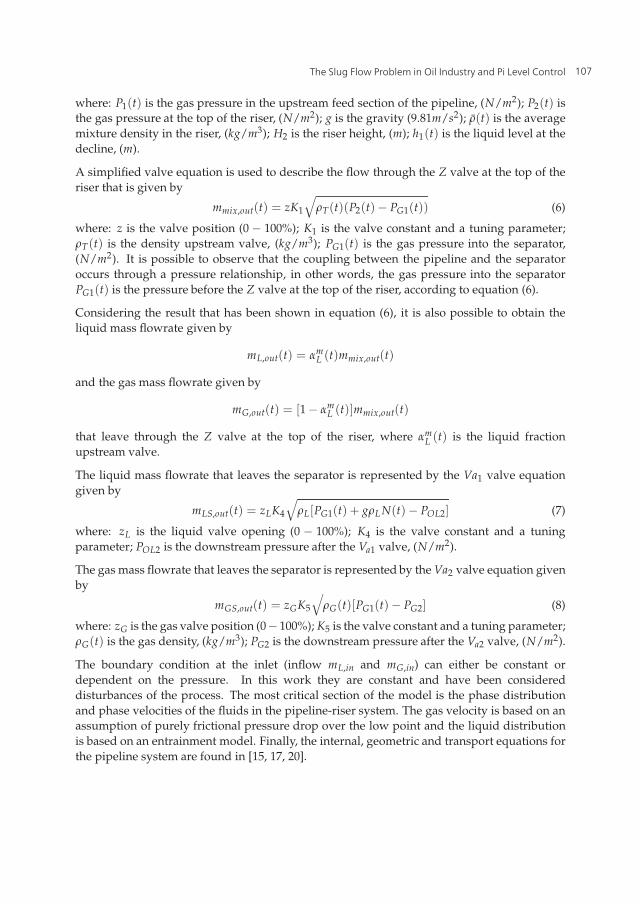
Figure 11. Liquid output flow rate variations mLS,out(t), (a) level control strategy PI conventional(dashed line) and level control strategy PI by band (solid line), (b) level control strategy PI conventional(dashed line) and error-squared level control strategy PI by band (solid line), z = 20%.

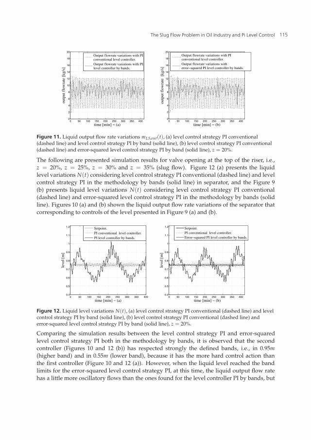
The following are presented simulation results for valve opening at the top of the riser, i.e.,z = 20%, z = 25%, z = 30% and z = 35% (slug flow). Figure 12 (a) presents the liquidlevel variations N(t) considering level control strategy PI conventional (dashed line) and levelcontrol strategy PI in the methodology by bands (solid line) in separator, and the Figure 9(b) presents liquid level variations N(t) considering level control strategy PI conventional(dashed line) and error-squared level control strategy PI in the methodology by bands (solidline). Figures 10 (a) and (b) shown the liquid output flow rate variations of the separator thatcorresponding to controls of the level presented in Figure 9 (a) and (b).

0 50 100 150 200 250 300 350 4000.4

0.5

0.6

0.7

0.8

0.9

1

1.1

1.2

time [min] − (a)

leve

l [m

]

Setpoint.PI conventional level controller.PI level controller by bands.

0 50 100 150 200 250 300 350 4000.4

0.5

0.6

0.7

0.8

0.9

1

1.1

1.2

time [min] − (b)

leve

l [m

]

Setpoint.PI conventional level controller.Error−squared PI level controller by bands.

Figure 12. Liquid level variations N(t), (a) level control strategy PI conventional (dashed line) and levelcontrol strategy PI by band (solid line), (b) level control strategy PI conventional (dashed line) anderror-squared level control strategy PI by band (solid line), z = 20%.

Comparing the simulation results between the level control strategy PI and error-squaredlevel control strategy PI both in the methodology by bands, it is observed that the secondcontroller (Figures 10 and 12 (b)) has respected strongly the defined bands, i.e., in 0.95m(higher band) and in 0.55m (lower band), because it has the more hard control action thanthe first controller (Figure 10 and 12 (a)). However, when the liquid level reached the bandlimits for the error-squared level control strategy PI, at this time, the liquid output flow ratehas a little more oscillatory flows than the ones found for the level controller PI by bands, but



0 50 100 150 200 250 300 350 4000

2

4

6

8

10

12

14

16

outp

ut f

low

rate

[kg

/s]

time [min] − (a)

Output flowrate variationswith PI conventional level controller.Output flowrate variations withPI level controller by bands.

0 50 100 150 200 250 300 350 4000

2

4

6

8

10

12

14

16

18

20

outp

ut f

low

rate

[kg

/s]

time [min] − (b)

Output flowrate variationswith PI conventional level controller.Output flowrate variations witherror−squared PI level controller by bands.

Figure 13. Liquid output flow rate variations mLS,out(t), (a) level control strategy PI conventional(dashed line) and level control strategy PI by band (solid line), (b) level control strategy PI conventional(dashed line) and error-squared level control strategy PI by band (solid line), z = 20%.

this difference is minimal, according to Figures 11 (a) and (b), Figures 13 (a) and (b). For bothcontrollers simulation results of the liquid output flow rate are better than the results obtainedwith the level control strategy PI conventional. Considering the liquid output flow rate whenthe level is within the band, both processes (i.e., level control strategy PI and error-squaredlevel control strategy PI both in the methodology by band) have similar trends.

6. Conclusion

In this chapter with objective of reducing the export oscillatory flow rate caused by slugflow, three methodologies of the level controls were implemented (1) level control strategyPI conventional; (2) level control strategy PI in the methodology by bands; (3) error-squaredlevel control strategy PI in the methodology by bands.

The simulation results showed that the error-squared level control PI strategy in themethodology for bands presented the better results when compared with the level controlstrategy PI conventional, because reduced flow fluctuations caused by slug flow; and with thelevel control strategy PI in the methodology by bands, it probably happened because the firsthas highly respected the defined bands.

As suggestions for future work new control strategies can be implemented in integratedsystem, i.e., more than one valve simultaneously. Considering the mathematical modelingof the process, it was necessary to investigate a mathematical model with fewer parameters,along with the construction of an experimental platform, since the data of a real process isdifficult to obtain and are not provided by oil industry.

Author details

Airam Sausen, Paulo Sausen, Mauricio de CamposMaster’s Program in Mathematical Modeling (MMM), Group of Industrial Automation and Control,Regional University of Northwestern Rio Grande do Sul State (UNIJUÍ), Ijuí, Brazil.



7. References

[1] Astrom, K. J. & Hagglund, T. [1995]. PID Controllers: Theory, Design, and Tuning, ISA,New York.

[2] Bendiksen, K., Malnes, D., Moe, R. & Nuland, S. [1991]. The dynamic two-fluid modelolga: theory and application, SPE Production Engineering, pp. 171–180.

[3] de Campos, M. C. M., Costa, L. A., Torres, A. E. & Schmidt, D. C. [2008]. Advancedcontrol levels of separators production platforms, 1 CICAP Congresso de Instrumentação,Controle e Automação da Petrobrás (I CICAP), Rio de Janeiro. in Portuguese.

[4] Friedman, Y. Z. [1994]. Tuning of averaging level controller, Hydrocarbon ProcessingJournal .

[5] Godhavn, M. J., Mehrdad, F. P. & Fuchs, P. [2005]. New slug control strategies, tuningrules and experimental results, Journal of Process Control 15: 547–577.

[6] Havre, K. & Dalsmo, M. [2002]. Active feedback control as a solution to severe slugging,SPE Production and Facilities, SPE 79252 pp. 138–148.

[7] Havre, K., Stornes, K. & Stray, H. [2000]. Taming slug flow in pipelines, ABB review,number 4, pp. 55–63.

[8] Havre, K. & Stray, H. [1999]. Stabilization of terrain induced slug flow in multiphasepipelines, Servomotet, Trondheim.

[9] Nunes, G. C. [2004]. Bands control: basic concepts and application in load oscillationsdamping in platform of oil production, Petróleo, Centro de Pesquisas (Cenpes), pp. 151–165.in Portuguese.

[10] Sausen, A. [2009]. Mathematical modeling of a pipeline-separator system unde slug flow andcontrol level considering an error-squared algorithm, Phd thesis, Norwegian University ofScience and Technology, Brazil. in Portuguese.

[11] Sausen, A. & Barros, P. R. [2007a]. Lyapunov stability analysis of the error-squaredcontroller, Dincon 2007 - 6th Brazilian Conference on Dynamics, Control and TheirApplications, São José do Rio Preto, Brasil, pp. 1–8.

[12] Sausen, A. & Barros, P. R. [2007b]. Properties and lyapunov stabilty of the error-squaredcontroller, SSSC07 - 3rd IFAC Symposium on System, Structure and Control, Foz do Iguaçu,Brasil, pp. 1–6.

[13] Sausen, A. & Barros, P. R. [2008]. Modelo dinâmico simplificado para umsistema encanamento-Riser-separador considerando um regime de fluxo com golfadas,Tendências em Matemática Aplicada e Computacional pp. 341–350. in Portuguese.

[14] Shinskey, F. [1988]. Process Control Systems: Application, Design, and Adjustment,McGraw-Hill Book Company, New York.

[15] Storkaas, E. [2005]. Stabilizing control and controllability: control solutions to avoid slug flowin pipeline-riser systems, Phd thesis, Norwegian University of Science and Technology,Norwegian.

[16] Storkaas, E., Alstad, V. & Skogestad, S. [2001]. Stabilization of desired flow regimes inpipeline, AIChE Annual Meeting, number Paper 287d, Reno, Nevada.

[17] Storkaas, E. & Skogestad, S. [2002]. Stabilization of severe slugging based ona low-dimensional nonlinear model, AIChE Annual Meeting, number Paper 259e,Indianapolis, USA.

[18] Storkaas, E. & Skogestad, S. [2005]. Controllability analysis of an unstable, non-minimumphase process, 16th IFAC World Congress, Prague, pp. 1–6.



[19] Storkaas, E. & Skogestad, S. [2006]. Controllability analysis of two-phase pipeline-risersystems at riser slugging conditions, Control Enginnering Practice pp. 567–581.

[20] Storkaas, E., Skogestad, S. & Godhan, J. M. [2003]. A low-dimensional dynamic model ofsevere slugging for control design and analysis, 11th International Conference on Multiphaseflow (Multiphase03), San Remo, Italy, pp. 117–133.

[21] Tengesdal, J. O. [2002]. Investigation of self-lifting concept for severe slugging eliminationin deep-water pipeline/riser systems, Phd thesis, The Pennsylvania State University,Pennsylvania.

[22] Thomas, P. [1999]. Simulation of Industrial Processes for Control Engineers, Butterworthheinemann.


The Slug Flow Problem in Oil Industry and Pi Level...

Documents

Transcript of The Slug Flow Problem in Oil Industry and Pi Level...