arX

iv:n

ucl-

th/0

6070

02v1

3 J

ul 2

006

The Skyrme Interaction in finite nuclei and nuclear matter

J. R. Stone1,2,3 and P.–G. Reinhard4,5

1 Department of Physics, University Oxford,Oxford OX1 3PU / United Kingdom

2 Physics Division, Oak Ridge National Laboratory,P.O. Box 2008, Oak Ridge, TN 37831, USA

3 Department of Chemistry and Biochemistry,

University of Maryland, College Park, MD 20742, USA4 Institut fur Theoretische Physik, Universitat Erlangen,

D-91054 Erlangen, Germany5 Joint Institute for Heavy Ion Research, Oak Ridge National Laboratory,

P. O. Box 2008, Oak Ridge, TN 37831, USA

Abstract

Self-consistent mean-field models are a powerful tool in the investigation of nuclear structureand low-energy dynamics. They are based on effective energy-density functionals, often formu-lated in terms of effective density-dependent nucleon-nucleon interactions. The free parametersof the functional are adjusted to empirical data. A proper choice of these parameters requiresa comprehensive set of constraints covering experimental data on finite nuclei, concerning staticas well as dynamical properties, empirical characteristics of nuclear matter, and observational in-formation on nucleosynthesis, neutron stars and supernovae. This work aims at a comprehensivesurvey of the performance of one of the most successful non-relativistic self-consistent method,the Skyrme-Hartree-Fock model (SHF), with respect to these constraints. A full description ofthe Skyrme functional is given and its relation to other effective interactions is discussed. Thevalidity of the application of SHF far from stability and in dense environments beyond the nuclearsaturation density is critically assessed. The use of SHF in models extended beyond the mean fieldapproximation by including some correlations is discussed. Finally, future prospects for furtherdevelopment of SHF towards a more consistent application of the existing and promisingly newlydeveloping constraints are outlined.

1 Introduction

1.1 General overview of nuclear structure models

There is a great variety of nuclear structure models at very different theoretical levels. At the mostfundamental level are ab initio theories which start from a nucleon-nucleon force as input [1] andcompute the equation of state for nuclear matter by diagrammatic techniques (for reviews see, e.g.,[2, 3]) or from low-energy quantum-chromodynamics (see e.g. [4, 5, 6, 7]). These microscopic approacheshave made considerable progress over the past decades. One is even performing ab initio calculationsfor finite nuclei, e.g. in the no-core shell model [8, 9, 10], coupled cluster calculations [11], or in theunitary correlator method [12]. Nonetheless, the actual precision in describing nuclear properties is still

1

limited, typically 5% precision when ab initio two-body forces are used[11] (better quality of about 1%can be achieved when invoking effective three-body forces). Moreover, the application to finite nucleiare computationally very demanding, e.g. the largest no core shell model calculations go at most upto A=20 [13]. Thus fully microscopic methods are presently not used for large-scale nuclear structurecalculations.

At the most phenomenological level are the macroscopic approaches which are inspired by the ideathat the nucleus is a drop of nuclear liquid, giving rise to the liquid-drop model (LDM) or the morerefined droplet model, for a recent review see e.g. [14]. With a mix of intuition and systematic expansionin orders of surface effects (the leptodermous expansion) one can write down the corresponding energyfunctional [15]. There remain a good handful of free parameters, i.e the coefficients for volume energy,symmetry energy, incompressibility, or surface energy. These have to be adjusted to a multitude ofnuclear bulk properties with the results that modern droplet parameterizations deliver an excellentdescription of average trends [16]. Actual nuclei, however, deviate from the average due to quantumshell effects, so that shell corrections have to be added. They are related to the level density nearthe Fermi surface and can be computed from a well tuned, empirical nuclear single-particle potential.Macroscopic energy plus shell corrections constitute the macroscopic-microscopic (mac-mic) approachwhich is enormously successful in reproducing the systematics of known nuclear binding energies [17].One has to admit, though, that the mac-mic method relies strongly on phenomenological input. Thisinduces uncertainties when extrapolating to exotic nuclei. Particularly uncertain is the extrapolationof the single-particle potential used in this model (Nilsson, Yukawa) because this is not determinedself-consistently but added as an independent piece of information.

An intermediate level of nuclear models consists in microscopic theories employing effective inter-actions or effective energy-density functionals. There exist two basically different approaches. On theone hand, one has large scale shell model calculations which aim at a fully correlated description ofground state and excitations up to about 10 MeV, for a review see e.g. [18]. These employ the wavefunctions of a single-particle basis from empirical shell model potentials complemented by experimentalsingle-particle energies. The effective interaction in the valence space (two-body matrix elements) istaken often from microscopic information, namely the G-matrix from ab initio calculations, with abit of final fine-tuning. Some calculations rely fully on a phenomenological adjustment of the matrixelements. On the other hand, there are the self-consistent mean-field models which aim at a prejudice-free, self-consistent determination of the nuclear ground state and low-energy collective dynamics. Thepresent review con concentrates on this latter class of models.

Self-consistent mean-field models, as compared to the mac-mic method, take one big step towards amicroscopic description of nuclei. They produce the appropriate single-particle potential correspondingto the actual density distribution for a given nucleus. Still, they cannot be regarded as an ab initio

treatment because the genuine nuclear interaction induces huge short-range correlations that are notnaturally included in a Hartree-Fock model. Self-consistent mean-field models deal with effective energyfunctionals [19, 20]. The concept has much in common with the successful density-functional theory forelectronic systems [21]. The difference is, however, that electronic correlations are well under control andthat reliable electronic energy-density functionals can be derived ab initio because the electron-electroninteraction is well known. The nuclear case is much more involved because the nucleon as such is acomposite particle and a nucleon-nucleon interaction is already an approximate concept. Thus, nuclearmany-body theories, as discussed above, have not yet reached sufficient descriptive power to serve asdirect input for effective mean-field models. They serve as guidance to develop the basic features ofthe energy-density functionals [19]. The open model parameters are adjusted phenomenologically. Thethree most prominent schemes are the Skyrme energy functional, traditionally called Skyrme-Hartree-Fock (SHF), the Gogny model, and the relativistic mean field model (RMF), for a recent review see[22]. The present review refers mainly to SHF whilst establishing occasionally relations to the two otherschemes (see also Section 2.4).

2

As said above, the self-consistent mean-field models lie between ab initio theories and the mac-micmethod. The link between ab initio and SHF is still under development, as will be discussed briefly inSection 2.4. The connection between SHF and the mac-mic method is much better developed. Thereare attempts from both sides. The extended Thomas-Fermi Skyrme interaction scheme (ETFSI) startsfrom SHF and derives an effective mac-mic model by virtue of a semi-classical expansion [23, 24]. Thishas been exploited up to a quantitative level [25]. From the macroscopic side there is an attempt toinclude more self-consistency by virtue of a Thomas-Fermi approach [26, 27]. The investigation of theselinks turns out to be useful to gain more insight into the crucial constituents of either model.

One of the concerns in applying mean-field models is uncertainty in the phenomenological determi-nation of the free parameters in the effective energy functionals [28]. Many tens of different parametersets have evolved in the course of the development. The main problem is that one does not have avail-able a one-to-one correspondence between individual parameters and a specific piece of experimentalinformation. It follows that there is a continuum of parameter sets which would fit the experimentwith a comparable degree of accuracy. One of the important tasks in the development of mean fieldmodels is to devise ways of constraining the free parameters of interaction used. For example, new datafrom exotic nuclei are an enormous help in that respect. One more recently identified benchmark isthe application of SHF to asymmetric nuclear matter [28]. This development is related to an increasingdemand for microscopic nuclear structure input into models of stellar matter, occurring in neutron starsand core-collapse supernovae. Realistic description of asymmetric nuclear matter under conditions ofextreme density, pressure and temperature poses a new constraint to nuclear theory. It offers an exten-sive laboratory for testing the applicability of effective mean field models, fitted to properties of finitenuclei close to the beta-stability line, to the limits of nuclear binding at the neutron and proton drip-line. The role of the SHF in providing such input to nuclear astrophysics models and its implication isdiscussed in this work.

The present review aims to survey the current status of SHF theory as applied in both nuclear andastrophysics areas. The basic concepts and formalism of the Skyrme approach, the choice of parametersand links to the other models of nuclear interactions are detailed in Section 2. Section 3 is devoted toapplications in finite nuclei divided into subsections covering static properties (3.1) (binding energies,spin-orbit effects, neutron radii, super-heavy elements and fission barriers), dynamic properties (3.2)(giant resonances, Gamow-Teller resonances, heavy ion collisions and rotational bands) and nucleosyn-thesis (3.3) (r-process and rp-process). These is a final subsection devoted to discussion of collectivecorrelations beyond the mean field (3.4) (large amplitude collective notion, soft modes and low energyquadrupole states). Section 4 focuses on nuclear matter and astrophysical applications with subsectionsdiscussing the relevance of SHF to construction of EOS for compact objects (4.2), the key properties ofnuclear matter, models of cold neutron stars (4.3) and hot matter in type II (core-collapse) supernovamodels. Constraints on parameters of SHF functionals are summarized in Section 5 and conclusionsare drawn in Section 6.

2 The Skyrme energy functional

2.1 A priori correlations

2.1.1 On the description of correlations

The ultimate goal of a theory is, of course, an ab initio description which starts from the basic micro-scopic understanding of the constituents of the system and predicts finally the properties of a complexcompound. The microscopic theory of nucleons and nuclei is quantum chromodynamics (QCD) usingquarks and gluons as constituents [29]. However, QCD is a very involved theory and it is alreadyformidable work to compute the properties of single nucleons or mesons. The description of a whole

3

nucleus is presently far out of reach. Approximate QCD at the level of a low-energy limit or chiralperturbation theory allows approach finite nuclei and nuclear matter and it has been applied with in-creasing success in recent years [4, 5, 6, 7]. It should be noted, however, that these ab initio theories stillallow for a few free parameters to achieve fine-tuning of the results. But the field is still in a developingstage and steady improvement may be expected.

Tradition nuclear ab initio theories start from nucleons and two-body interactions between them asthe basic building blocks. The interaction is determined from an exhaustive analysis of nucleon-nucleonscattering, see e.g. [1]. The aim is a microscopic description of the fully correlated nuclear state. Itis called correlated as opposed to the mean-field state (Slater determinant or BCS state) which is theprototype uncorrelated state. One distinguishes several types of correlations. Short-range correlationsare related to the hard repulsive core of the nuclear interaction which develops at short inter-nucleondistances below 0.5 fm. Long-range correlations are mediated by the pronounced nuclear resonancemodes, the giant resonances; they mediate correlations over distances because their propagator haslarge coherence length (longer than any existing nucleus). Finally, there are the collective correlationsinduced by the soft modes with large amplitude such as center-of-mass motion, rotation, or low-lyingquadrupole vibrations. Each one of these types of correlation requires its own approach. We willsummarize them briefly here. For an extensive review of these very different methods see [30].

The family of conceptually simpler approaches is based on an obvious ansatz for the correlatedmany-body wavefunction. Examples are the Jastrow ansatz [31], the exp(S) method [32], and theunitary correlator technique [12]. These three methods have, in principle, much in common but differin the details of the practical evaluation. They start from a closed expression for the wavefunction andevaluate the expectation values approximately by elaborate expansion techniques (often called coupledcluster expansion). They are designed to describe the short-range correlations associated with the seriesof two-particle-two-hole (2ph) excitations. A more general ansatz is used in the ‘no core shell model’(NCSM) calculations which have been developed recently, see e.g. [8]. Here one aims at an expansion ofthe exact many-body wavefunction in a basis of given shell model wavefunctions. This method shouldin principle embrace all correlations, short as well as long range and to some extent also collective ones.

Alternatively to the NCSM , one has the diagrammatic techniques which are derived most often fromthe hierarchy of many-body Greens functions [33]. The short-range correlations are related to the seriesof ladder diagrams. The most widely used method is here the Brueckner-Hartree-Fock (BHF) theory, fora recent review see [2] and for its relativistic cousin, Dirac-Brueckner-Hartree-Fock (DBHF) models [34].The long-range correlations stem from the series of bubble diagrams (polarization propagators). Theyplay the dominant role in electronic systems [21]. There exist also noteworthy polarization correlationsin a nuclear environment, e.g., from the various giant resonance modes [35, 36]. A combined treatment ofshort- and long-range correlations has been tried in the theory of parquet diagrams [37]. The enormouscomplexity of these methods has so far hindered widespread applications of this approach. In practice,diagrammatic ab initio calculations in nuclear physics deal only with the short-range correlations. Thatis to some extent legitimate because they yield by far the dominant contributions due to the hugeshort-range repulsion in the nucleon-nucleon interaction.

Collective correlations require very different methods. The effect of zero-energy modes (center-of-mass, rotation, particle-number) is handled by projection [38]. Low energy modes, as e.g. quadrupolefluctuations, are usually treated by the generator-coordinate method (GCM) [39] and approximationstherein [40]. Other methods to deal with large amplitude motion in a wavefunction picture are re-quantized time-dependent Hartree-Fock (TDHF) or path integrals [41, 42, 43]. Alternatively, one candescribe a system in terms of operator algebra and large amplitude motion is covered here by bosonexpansion techniques [44].

The above short summary indicates that collective correlations differ strongly from short- and long-range correlations and appear at a different level of description. The collective correlations are relatedto shape and surface of finite nuclei and are very sensitive to shell effects which makes them vary

4

strongly from nucleus to nucleus. On the other hand, short- and long-range correlations are fullyactive in the nuclear volume and persist up to nuclear matter. Their effect is smoothly varying withproton and neutron number. The latter feature justifies summarizing these correlations implicitly inan effective energy-density functional, or effective interaction respectively. The way this is done andits consequences is sketched in the following subsections. The main message to be kept in mind isthat these short- and long-range correlations have been a priori built into the mean-field model andthey should not be computed again with these effective interactions (although there exist techniques torecover carefully some of those correlations in the T -matrix approach [45]). The collective correlations,on the other hand, cannot be transferred to a simple effective functional because they do not obeysmooth trends and rather vary strongly with proton and neutron number. They need to be left for a

posteriori treatment. The danger of double counting correlations is small because strongly fluctuatingeffects cannot be included already in a smooth energy functional. Examples for collective correlationswill be discussed in Section 3.4.

Finally, we want to address again the limitations of ab initio in a nuclear context. The startingassumption of nucleons as basic constituents is only approximately correct. It is then no surprise thatall strict ab initio calculations starting from measured nucleon-nucleon interactions fail to reproducenuclear binding and radii at a quantitative level (with typical errors of about 5% [46]). This fact hasinhibited so far a parameter-free deduction of effective energy-functionals. The quality of ab initio

calculations can be significantly enhanced by introducing effective three-body forces. These, however,introduce free parameters in the treatment which spoil the ideal of an ab initio derivation. As aconsequence, the free parameters of nuclear energy-density functional are directly fitted to empiricaldata, see Section 2.3.

2.1.2 Motivation of the Skyrme functional

The formally most transparent way to explain the construction of an effective interaction is providedby the unitary correlator method. The fully correlated state is written as a unitary transformation Uof a mean field state |Φ〉, i.e.

|Ψ〉 = U |Φ〉 . (1)

At the lowest level, the unitary transformation is composed from exponentiated two-body correlations

U = exp(

ı∑

cabcda+a a+

b acad

)

(2)

where a+, a are Fermion operators [12]. The energy expectation value is regrouped as

E = 〈Ψ|H|Ψ〉 = 〈Φ|U+HU |Φ〉 = 〈Φ|Heff |Φ〉 . (3)

This defines the effective Hamiltonian

Heff = U+HU . (4)

by associating the correlators to the Hamiltonian. Note that the expectation value with Heff is welldefined only in connection with mean-field states |Φ〉 and for nothing else. The price for the ‘effective-ness’ is the restriction of the legitimate Hilbert space. Such restrictions are best handled in variationalformulations and it is thus natural that effective mean-field models come along in this fashion. Thus farthe principle of building an effective interaction looks simple and is well established in the derivation ofeffective charges (for a discussion in diagrammatic terms see [47]). The practical evaluation, however,is extremely tedious and not very enlightening.

More details about the desirable structure of a Skyrme-like effective functional are disclosed by thetechnique of the density-matrix expansion [48]. Many ab initio models deliver at the end an effective

5

two-body interaction as an involved integral operator G. This holds, in particular, for the Bruckner-Hartree-Fock method (BHF) whose G-matrix serves finally as effective force for the Hartree-Fock part,for a recent review see e.g [2]. An effective force as integral operator can also be extracted from manyother ab initio models, as e.g. the above mentioned unitary correlator method. In any case, the mostgeneral total energy becomes

Epot =

∫

dx dx′dy dy′ρ(x, x′) G(x, x′; y, y′) ρ(y, y′) (5)

where ρ(x, x′) is the one-body density matrix which falls off quickly with increasing |x − x′| with atypical range of k−1

F where kF is the Fermi momentum. More importantly, the integral kernel G is alsonon-zero only for small differences in all pairs of coordinates with typical ranges mostly below k−1

F . Thissuggests an expansion in orders (x− x′)n around x = (x + x′)/2 in the form

ρ(x, x′) ≈ n(x) + i(x− x′) · j(x) +1

2(x− x′)2

(

τ −1

4∆n)

, (6)

where n is the local density, j the local current, and τ the kinetic-energy density, see Section 2.2.1.It is obvious that this expansion in x − x′ and similarly in y − y′ yields properly the τ terms in thefunctionals. The G matrix is also well localized in the differences x−y and x′−y′. An expansion of theG matrix with respect to these differences yields the gradient terms ∝ ∆n in the effective functional.Altogether, the density-matrix expansion demonstrates how a zero-range effective interaction emergesfrom the initially given involved operator structure. We are dealing with a typical low-energy or low-q expansion. It becomes apparent that this puts even more constraints on the legitimate mean-fieldstates. The spatial structure should be sufficiently smooth. A safe estimate takes the pion wavelengthas the largest range in G. This complies with the spatial variations in the wavefunctions and densitiesof order of k−1

F at normal nuclear density. The validity of effective functionals exceeds often the rangeof such safe estimates. But one should be warned about extension to high densities. Sooner or later,effective functionals of zero range will become inappropriate. There exist methods to extend the rangeto a broader span of densities which have been worked out, e.g., for 3He systems [49] but not yet fornuclear systems.

Density functional theory provides the conceptually and technically simplest way to derive an energy-density functional from ab initio calculations. This is the much celebrated local-density approximation(LDA) [21]. We sketch it briefly for the case of one component. A nuclear LDA deals, of course, withtwo components, for protons and for neutrons separately. The basic steps can be summarized as follows:

n =⇒E

N=ǫ(n) =⇒ E =

∫

d3r nε(

n) n→n(r)

=⇒ E(LDA) =

∫

d3r n(r)ε(

n(r))

. (7)

One performs first a series of ab initio calculations in bulk matter for many different (homogenous)densities n. This yields an energy per particle E/N as function of n. It is rewritten as a spatial integralwhich is still exact for homogenous densities. The crucial step comes when allowing for spatiallyvarying densities n −→ n(r). This assumes that the finite and inhomogeneous system can be treatedas a succession of pieces of bulk. This is an approximation for sufficiently smooth density distributions.What “sufficiently smooth” means in practice remains an open question as has been discussed alreadyat the end of the previous paragraph. We will reconsider that question with a realistic application inSection 2.4.3.

2.2 The composition of the energy functional

2.2.1 The wavefunctions and densities

The key idea in a mean field theory is that one seeks to describe the many-body system exclusively interms of a set of single-particle wavefunctions ϕα, α = 1, ..., A. These constitute the many-body state

6

as a Slater determinant which is the anti-symmetrized product of all occupied single-particle states. Apure Slater state is simply applicable only to doubly-magic nuclei which, however, are a small minorityin the table of isotopes. All others have partially open shells with a high density of almost degeneratedstates which gives the residual two-body interaction a chance to mix these states in order to producea unique ground state [50]. This can be handled very efficiently and to a reasonable approximationby a nuclear pairing scheme, see e.g. [38, 22] for details. At the end, this amounts associating anoccupation amplitude vα with each single-nucleon state ϕα. This amplitude can take values continouslyin the interval [0, 1]. The complementary non-occupation amplitude is uα =

√

1− v2α. Thus the typical

mean-field state is a BCS state|Φ〉 = Πα

(

uα + vαa+αaα

)

|0〉 (8)

where |0〉 is the vacuum state. This BCS state comprises all the information carried in the setϕα, vα; α=1, ..., Ω. The limit Ω > A denotes the size of the pairing-active space The dynamicaldegrees-of-freedom are the single-particle wavefunctions ϕα and the occupation amplitudes vα. Themean field equations are obtained by variation of the total energy with respect to these both quanti-ties. The expression for the total energy is the key ingredient in the modeling. We will employ herethe Skyrme energy-density functional as given in Section 2.2.2 together with a pairing functional, seeSection 2.2.4. The equations for the Hartree-Fock mean field are obtained by variation with respect tothe wavefunctions ϕα while the gap equations for the pairing mean field come from variation of the vα.

Wavefunctions and occupations amplitudes uniquely define all one-body densities. Energy-densityfunctionals should require the knowledge of only a few local densities and and currents, such as the localdensity n(r). For nuclei, we have to distinguish proton and neutron density, np and nn. Note that weare using here the symbol n for the local particle number density. This differs from the standard usagein the SHF community of the symbol ρ for this quantity. But it complies with the usage in nuclearastrophysics where the symbol ρ is reserved for the mass density (see Section 4.2), and it agrees alsowith the standards of electronic density-functional theory [21]. Furthermore, nuclear energy functionalsinvoke also the kinetic-energy density τ , the spin-orbit density J, the current j, the spin density σ, andthe kinetic spin density τ . These read in detail

nq(r) =∑

α∈q

∣

∣v2α

∣

∣

∣

∣ϕα(r)∣

∣

2q ∈ p, n , (9a)

τq(r) =∑

α∈q

∣

∣v2α

∣

∣

∣

∣∇ϕ(r)∣

∣

2, (9b)

Jq(r) = −ı∑

α∈q

∣

∣v2α

∣

∣ϕ+α (r)∇×σϕα(r) , (9c)

jq(r) = −ı

2

∑

α∈q

∣

∣v2α

∣

∣

(

ϕ+α (r)∇ϕα(r)−∇ϕ+

α (r)ϕα(r))

, (9d)

σ(r) =∑

α∈q

∣

∣v2α

∣

∣ϕ+α (r)σϕα(r) , (9e)

τ (r) =∑

α∈q

∣

∣v2α

∣

∣

∑

i∈xyz

∇iϕ+α (r)σ∇iϕα(r) . (9f)

It is often useful to recouple to sum and difference, e.g.

n = np + nn , n = np − nn , (9g)

and similarly for all other densities and currents. The sum plays a role in the isoscalar terms of theenergy functional and we will call it the isoscalar density n. In a similar manner, the difference playsthe role of an isovector density n.

7

2.2.2 Basic formalism

The Skyrme force was first introduced by Skyrme in [51, 52] as an effective force for nuclear Hartree-Fockcalculations. Its widespread application started with the revival by Vautherin and Brink in [53, 54]. Itused to be formulated as an effective interaction

Veff(r1, r2) = t0(1+x0Pσ)δ(r1−r2) +t36

(1+x3Pσ)δ(

(12(r1+r2)

)

δ(r1−r2)

−t12

(1+x1Pσ)(

(∇1−∇2)2δ(r1−r1) + h.c.

)

−t3(1+x2Pσ)(

(∇1−∇2)δ(r1−r2)(∇1−∇2))

−ıt4(∇1−∇2)×δ(r1−r2)(∇1−∇2))

·(σ1+σ2) , (10)

Pσ =1

2(1 + σ1 ·σ2) ,

where Pσ is the spin-exchange operator. It is a zero-range interaction with kinetic and density-dependentterms. The zero range is an idealization which is consistent with the smoothly varying dependence ofthe mean field state on spatial coordinates. Such a force makes sense only in connection with suchsmooth wavefunctions and should never be used to regenerate short-range correlations [53]. The densitydependent term ∝ t3 is of particular importance as it provides appropriate saturation and thus securesthe success of SHF in description of finite nuclei. It is motivated by the concept of effective forcesbetween nucleons in nuclear environment in contrast to the forces between bare nucleons. It can beseen as arising from either the concepts of effective forces or energy functionals, resulting from thevariation with density of the underlying microscopic effective interaction or of the energy (see [48] andSection 2.1.2). It was originally formulated as a zero-range three-body force which is equivalent to thedensity-dependent interaction (DDI) when used in calculations of ground state properties. However,the two interpretations of the ∝ t3 differ when excitations are considered and the DDI approach isfound to be more stable [55]. On the other hand, the concept of a DDI leads to inconsistencies in avariational formulation in that the variationally derived two-body interaction is not identical to theinitially given interaction from which the energy was computed as expectation value. What is done inpractice, is to compute the total energy as expectation value of the interaction first (10) and then derivethe Hartree-Fock equations and solve them using the standard variational procedure. This is preciselythe concept of an effective energy-density functional. And this is the line of development which we willpursue in the following.

Our starting point is then the most general Skyrme energy functional which reads

E =

∫

d3r n Ekin + ESkyrme + ESkyrme,odd+ ECoulomb + Epair + Ecm , (11a)

nEkin =~

2

2m

∫

d3 τ , (11b)

nESkyrme =B0 + B3n

α

2n2 −

B′0 + B′

3nα

2n2

+B1

(

nτ − j2)

−B′1

(

nτ − j2)

−B2

2n∆n +

B′2

2n∆n

−B4n∇·J− (B4+B′4)n∇·J +

C1

2J2 −

C ′1

2J2 , (11c)

nESkyrme,odd = −C0 + C3n

α

2σ

2 +C ′

0 + C ′3n

α

2σ

2 +C2

2σ ·∆σ −

C ′2

2σ ·∆σ

−C1σ ·τ + C ′1σ ·τ − B4σ ·(∇×j)− (B4+B′

4)σ ·(∇× j) , (11d)

ECoulomb = e2 1

2

∫

d3r d3r′np(r)np(r′)

|r− r′|−

3

4e2

(

3

π

)1/3 ∫

d3r[

np

]4/3. (11e)

8

The B (B′) parameters determine the strength of the isoscalar (isovector) forces. The spin-orbit term∝ B4, B

′4 has only one free parameter B4 in the standard Skyrme functionals where one fixes B′

4 = 0.The need for full isovector freedom in the spin-orbit term, i.e. for a non-zero B′

4, was raised by thesystematics of isotopic shifts in Pb isotopes [56]. The principle Skyrme functional ESkyrme contains justthe minimum of time-odd currents and densities which is required for Galileian invariance [57], namelythe combinations nτ − j2 and n∇·J + σ ·(∇×j) . Further conceivable time-odd couplings are collectedin the optional terms in ESkyrme,odd. In case of a derivation from the zero-range two-body force (10),they are related to the B parameters of ESkyrme and the relation is given implicitly in eq. (12). Allthese C-terms are optional from the perspective of a pure energy-density functional and they are notyet well determined. The pure spin terms ∝ C0, C2 play a role only in truly time-odd situations suchas, odd-A nuclei or the Gamow-Teller excitations (see Section 3.2.2); they are not yet well investigated.The tensor spin-orbit terms ∝ C1, C

′1 can contribute in most standard situations although no specific

consequence of their inclusion or need for them has not yet been unambiguously identified. The Coulombfunctional (11e) depends only on the charge density and stays outside this distinction. Its second termapproximates exchange in the Slater approximation [58]. Note that we use the proton density in placeof the charge density. This is a widely used, more or less standard, approximation. The center of mass(c.m.) term Ecm will be discussed in Section 2.2.3 and the pairing energy Epair in 2.2.4.

The energy-functional (11) leaves the time-odd part (11d) open for free adjustment. The viewpointof an effective interaction as formulated in eq. (10) establishes unique relations between the frequentlyused interaction parameters ti, xi and the functional parameters Bi, Ci:

B0 = 34t0 , B′

0 = 12t0(0.5 + x0) ,

B1 = 316

t1 + 516

t2 + 14t2x2 , B′

1 = 18

[

t1(0.5 + x1)− t2(0.5 + x2)]

,

B2 = 932

t1 −532

t2 −18t2x2 , B′

2 = 116

[

3t1(0.5 + x1) + t2(0.5 + x2)]

,

B3 = 316

t3 , B′3 = 1

8t3(0.5 + x3)

B4 = b4 − 0.5b′4 , B′4 = 0.5b′4 , (12a)

C0 = −0.5t0(

0.5− x0

)

, C ′0 = 1

4t0 ,

C1 = 18

[

t1(

0.5− x1

)

− t2(

0.5 + x2

)

]

, C ′1 = − 1

16(t1 − t2) ,

C2 = − 116

[

3t1(

0.5− x1

)

+ t2(

0.5 + x2

)

]

, C ′2 = 1

32(3t1 + t2) ,

C3 = −18t3(0.5− x3) , C ′

3 = 116

t3 , (12b)

There is a one-to-one correspondence between the B and the t, x-parameterizations. The C-parametersare a consequence of the interaction ansatz and can in this connection be considered as function ofthe Bs. At first glance, this feature looks like an advantage of the interaction model. However, thisimposed restrictions may lead to conflicting requirements as worked out in Section 3.1.2 in connectionwithe isovector spin-orbit force. The zero-range two-body spin-orbit interaction in the ansatz (10) forcesB′

4 = 0 while the energy functional takes B′4 as a free parameter which is found desirable to be adjusted

independently.Empirical information for the other terms in the time-odd part (11d) is much harder to obtain.

These terms are not active in the ground state of even-even nuclei. Odd nuclei could supply usefulinformation, however mixed with pairing properties [59]. This has not yet been explored in a systematicmanner. Excitations probe time-odd terms and the spin-couplings are particularly crucial in modes withunnatural parity, see Section 3.2.2. Again, this is an area where systematic explorations are still ahead.Theoretical assistance can be obtained from the RMF where spin properties are fixed by the Dirac

9

equation. A study of the non-relativistic limit suggests a minimalistic model Ci = 0 [60] which deliversthe correct isovector structure for the spin-orbit coupling [56].

2.2.3 The center of mass correction

Electron clouds in an atomic or molecular system are bound by the external Coulomb forces of theionic background. Nuclei are different in that their center of mass moves freely through space withoutconfining fields (at least at nuclear scale). Thus the nuclear ground state should be projected on center-of-mass (c.m.) momentum zero [38]. The exact projection is tedious and a hindrance to large scalecalculations. Fortunately, the c.m. projection is well behaved and can be approximated by simpleexpressions [61]. Two different approximate expression for the c.m. correction are in use:

Ecm = E(full)cm = −

1

2mA〈(

∑

i

pi

)2〉 , (13a)

Ecm = E(diag)cm = −

1

2mA〈∑

i

p2i 〉 , (13b)

where the brackets mean the expectation value over the BCS state (8). The full correction (13a) is asecond order approximation to the exact c.m. projection and works very well for nuclei with A ≥ 40and is still a fair approximation for lighter nuclei [61]. It encompasses effectively a two-body operatorwhich adds complications to the variational mean field equations. Thus it is usually added a posteriori,i.e. after the solution of the mean field equations (projection after variation). The correction (13b)takes only the diagonal parts of the two-body operator and so yields a one-body operator. This allowsit to be included in the mean field equations (variation after projection) which is the standard for thatvariant of the theory. However, the form (13b) is a rather poor approximation to the full correction(13a) and should be avoided. An attempt to cure the defects of this approach by a simple fit formulawas made in [62] where the term (13b) is augmented by a factor f(A) = 2/(t + 1/3t) with t = (3

2A)1/3.

There is also a center-of-mass correction for the nuclear density distribution and quantities deducedtherefrom. This will be discussed in Section 2.2.6.

2.2.4 Pairing interaction

Pure Slater states are distinguished by occupation weights nα ∈ 0, 1. Such states are appropriate,however, only for doubly magic nuclei. All others have partially open shells with a high density ofalmost degenerated states which gives the residual two-body interaction a chance to mix these states inorder to produce a unique ground state [50]. This can be handled very efficiently and to a reasonableapproximation by a nuclear pairing scheme, see e.g. [38, 22] for details. In the end, this amounts toassociating an occupation amplitude vα ∈ 0, 1 with each single-nucleon state ϕα. The complementingnon-occupation amplitude is uα =

√

1− v2α. Assuming a zero-range residual interaction leads to the

pairing energy functional

Epair = E(DI)pair =

1

4

∑

q∈p,n

V (pair)q

∫

d3rχ2q , χq(r) =

∑

α∈q

wαuαvα|ϕα(r)|2 , (14a)

where DI stands for δ-interaction and wα is some phase-space weight. This pairing acts without prejudicethroughout the whole nuclear volume. There are good reasons to assume that most of the pairing takesplace near the nuclear surface [63]. That is accounted for by the density-dependent δ-interaction (DDDI)with the functional [64]

Epair = E(DDDI)pair =

1

4

∑

q

v0,q

∫

d3rχ2q

[

1−

(

n

n0

)γ ]

, (14b)

10

where n0 is the nuclear saturation density, typically n0 = 0.16 fm−3 and γ models the surface profile ofthe interaction. A standard value is γ = 1. For a discussion of the effects of varying γ see, e.g., [65].The two forms of the pairing functional (14a,14b) are practically standard in modern SHF calculations.

The strength parameters V(pair)p and V

(pair)n are universal in that they can be adjusted to hold for the

whole nuclear landscape. There are more elaborate treatments using the pairing part of the Gognyforce [66] which is, of course, compulsory in Gogny mean-field calculations and which is also often usedin RMF approaches, see e.g. [67]. Most older calculations use simpler schemes for pairing such as, aconstant pairing matrix element of a constant gap [68, 67]. These recipes depend very sensitively onthe pairing phase space and their parameters change substantially over the nuclei. They do not meetthe high standards of modern mean field calculations.

The results of HFB or HFBCS calculations (see Section 2.2.5) depend on the space of single-nucleonstates taken into account, called here pairing phase space. The convergence with increasing phasespace is extremely slow [69] so some cut-off procedure is compulsory to obtain a manageable scheme.In fact, the cut-off is part of the pairing description. It is provided by the phase-space weights wα

in the above pairing functionals. The simplest way is to use a sharp cut with wα ∈ 0, 1. Thisworks well in connection with large pairing spaces reaching up to 50 MeV above the Fermi surface [70].Practicability often requires cuts at lower energy. The sharp cutoff then raises ambiguities if the leveldensity near the cutting edge is high. Much more elegant and stable is a soft cutoff profile such as,wα = [1 + exp ((εα − (ǫF + ǫcut))/∆ǫ)]−1 where typically ǫcut = 5 MeV and ∆ǫ = ǫcut/10 [71, 72]. Thisworks very well for all stable and moderately exotic nuclei. For better extrapolability away from thevalley of stability, the fixed margin ǫcut may be modified to use a band of fixed particle number ∝ N2/3

instead of a fixed energy band [73].A basic problem with pairing is particle-number conservation. The BCS state (8) is adjusted to

reproduce the correct average number of protons and neutrons. But it comes with some uncertaintyin proton and neutron number as soon as uαvα 6= 0. This uncertainty is embodied in the mean fieldapproximation. Nonetheless, one often sees a need for restoring exact particle numbers. This canbe achieved by particle-number projection [38] although this is a bit cumbersome and, even worse, isnot necessarily consistent in connection with energy-density functionals [74]. As in the case of c.m.projection, one can resort to approximate projection which is done usually in terms of the Lipkin-Nogami (LN) prescription (for a detailed discussion with comprehensive references see [22]). Most ofthe results presented here use simple BCS or HFB unless otherwise indicated.

2.2.5 The mean field and pairing equations

The energy functional (11) once fully specified determines everything. The mean field plus pairingequations are obtained in a straightforward manner. Variation with respect to the single-nucleonwavefunctions ϕ+

α yields the mean-field equations and variation with respect to the occupation am-plitudes vα provides the Bogoliubov equations, both together comprising the Hartree-Fock-Bogoliubovscheme (HFB). In practice, the feedback of vα variation on the mean field is neglected, yielding theBardeen-Cooper-Schrieffer (BCS) approximation to pairing. We skip the detailed mean field and pairingequations for reasons of brevity. A comprehensive description is found in the recent review [22].

Numerical implementation of the HFB(CS) equations requires further consideration. There aretwo different ways to represent wavefunctions and fields. On the one hand are the basis expansionswhich usually employ harmonic oscillator wavefunctions (for a recent detailed application see [75]). Onthe other hand are grid techniques where the wavefunctions and fields are represented on a grid incoordinate space. Depending on the symmetry, this can be a radial 1D, an axial 2D, or a Cartesian 3Dgrid. Coordinate-space grids are well suited for self-consistent mean fields which employ local densities.For the kinetic energy, various approximations are available: Fourier representation or finite differenceformulae at various orders. The optimum choice depends on the dimensionality, see e.g. [76]. A detailed

11

example of implementation on a spherical one-dimensional grid is presented in [77].

2.2.6 Computation of basic observables

The most prominent observable is, of course, the total energy. It is the starting point of the descrip-tion (see Section 2.2.2) and thus naturally results from any mean field calculation. The best possiblereproduction of the energies is, of course, the most important feature in the development of the model,see Section 2.3.1. A more refined view emerges when looking at energy differences which may revealinformation on the underlying shell structure (see Section 3.1.1) or lead to effects beyond a mere mean-field description (see Section 3.4). A further energy-related quantity is the single particle spectrum. Itis a natural outcome of mean field calculations. There is, however, no direct relation to experimentalobservables. One usually deduces single particle energy from neighboring odd-A nuclei which meansthat the results are masked by polarization and correlation effects. But differences of single-particleenergies, in particular spin-orbit splittings, can be extracted fairly well [78].

Next to the energy, the density distribution is a key feature of nuclear structure. Elastic electronscattering allows a more or less model free experimental determination of the nuclear charge formfactorFch(k) [79]. The formfactor is related to the density by a simple Fourier transformation Fq(~k) =∫

d3r exp ı~k ·~rnq(~r) where the variable index q ∈ ch,p,n indicates that this one-to-one relation holds for

any distribution, charge, proton or neutron like. It depends only on k= |~k| for spherical systems. We willbase the following discussion on the less intuitive but formally simpler formfactor and assume sphericalsymmetry. Mean field calculations yield proton and neutron formfactors. The charge formfactor isobtained by multiplying these with the intrinsic proton and neutron formfactors (equivalent to foldingof the densities) [80]

Fch(k) =∑

q

[FqGE,q + Fls,qGM ] exp

(

~2k2

8〈~P 2

cm〉

)

(15)

where Fls,q is the form factor of ∇ · ~Jq augmented by a factor µq/4m2 with µq being the magneticmoment of the nucleon, GE,q is the electric form factor and GM the magnetic form factor of the nucleons(assumed to be equal for both species). The overall exponential factor takes into account the center-of-mass correction for the formfactor complementing the corresponding energy correction as discussed inSection 2.2.3. It employs the same variance of the total momentum 〈P2

cm〉 and its physical interpretationis an unfolding of the spurious vibrations of the nuclear center-of-mass in harmonic approximation [61].The nucleon form factors GE,q and GM are taken from nucleon scattering data [81, 82], for details see[22].

Energy density functionals should, in principle, provide a reliable description of all density distri-butions, or, equivalently, formfactors. Actual functionals employ analytically simple forms which aresmooth functions of the densities as motivated by a local-density approximation. It has been shownthat this limits the predictive value to the regime k < 2kF in the formfactor where kF is the Fermimomentum [83]. Fortunately, the salient features of the nuclear shape are determined in that low krange. They can be characterized in terms of three form parameters: r.m.s. radius rch, diffraction radiusRch, and surface thickness σch [79]. They are computed as [79]

rch =3

Fch(0)

d2

dk2Fch(k)

∣

∣

∣

∣

k=0

, (16a)

Rch =4.493

k(1)0

, Fch(k(1)0 ) = 0 (16b)

σch =2

km

log

(

Fbox(km)

Fch(km)

)

, Fbox(k) = 3j1(kmRch)

kmRch

, km = 5.6/Rch (16c)

12

The diffraction radius Rch parameterizes the overall diffraction pattern which resembles these of afilled sphere of radius Rch. It is called the box equivalent radius [79]. The actual nuclear form factordecreases faster than the box form factor Fbox due to the finite surface thickness σ of nuclei which isthus determined by comparing the height of the first maximum of the box equivalent form factor and

of the mean-field result Fch. The simple simple combination√

35R2

ch + 3σ2ch − rch of these three form

parameters serves as a nuclear halo parameter which is found to be a relevant measure of the outersurface diffuseness [84].

The charge distribution is mostly sensitive to the proton distribution. Useful complementing infor-mation is contained in the neutron distribution which is discussed briefly in Section 3.1.3.

2.3 Basic features

The form of the energy functional as presented in Section 2 is based on a low momentum expansion ofmany-body theory [48] which leads naturally to local point couplings with some density dependence.The parameters of the functional are universal in the sense that they apply unmodified to all conceivablenuclei however they have to determined by fit to experimental data since nuclear many-body theoriesare not yet precise enough to allow an ab initio computation of nuclear properties with the precisionwhich we need for practical applications. Thus it is still state of the art to adjust the parameters of thefunctional phenomenologically. Typical strategies for the adjustment will be discussed in Section 2.3.1and its practical consequences subsequently. Thereby we include also the RMF in the considerationsas the relativistic cousin of SHF because similarities and differences between SHF and RMF are oftenquite instructive. The connection to BHF and the importance of each parameter is discussed briefly in2.4.3.

2.3.1 Fitting strategies

The parameters of the functional are adjusted such that a certain set of observables is optimally repro-duced. Different groups have different biases in selecting these observables. Fits are usually restrictedto a few semi- or doubly-magic spherical nuclei (an exception is a recent large-scale fit to all knownnuclear masses [85]). All fits take care of binding energy EB and r.m.s. charge radii rch after whichdifferent tracks are pursued. SHF fits include extra information on spin-orbit splittings while RMFincorporates the spin-orbit interaction automatically as a relativistic effect, see Section 2.4.1. Pairingproperties are usually adjusted to the odd-even staggering of binding energies, see e.g. [86, 73]. Somefits add information on nuclear matter, the series [87] even on neutron matter. Others make a pointto include information from the electromagnetic formfactor [88] (see Section 2.2.6). Differences existalso in the bias and weight given to the various observables; e.g., the force BSk1 fits exclusively tobinding energies (≡ atomic masses). Recently, attention has been brought to possible corrections forproton-neutron correlations in N = Z nuclei, often called the Wigner energy [89] (see e.g. the fits of[85]). A detailed discussion of fitting strategies can be found, e.g., in [22].

In view of these different prejudices entering the fits, there exist many different parameterizationsfor SHF as well as RMF. We confine the discussion to a few well adjusted and typical sets. They aresummarized together with their citations, actual options, and fit bias (last two columns) in Table 1. Afew further explanations are in order. They expand mainly the key words in the column ‘comments’.SkM∗ belonged to the second generation of Skyrme forces which delivered for the first time a wellequilibrated high-precision description of nuclear ground states. It was developed with an explicitstudy of surface energy and fission barriers in semiclassical approximation. SkP aimed at a simultaneousdescription of the mean field and of pairing. The set SLy6 and its cousins (see [87]) have been developedwith a bias to neutron rich nuclei and neutron matter aiming at astrophysical applications. SkI3 andSkI4 exploit the freedom of an isovector spin-orbit force to obtain an improved description of isotopic

13

force ref. c.m. l*s T=1 ηls Coul.ex. nuc.mat. commentsSkM∗ [90] diag no no yes yes fission barriersSkP [70] diag no no yes yes pairingSLy6 [87] full no no yes yes neutron matterSkI3/4 [56] full yes no yes no isotopic shift PbBSk1 [85] diag no no yes no deformed nucleiPC-F1 [91] full no noNL-Z [92] diag no noNL3 [93] guess no yes isovector bias

Table 1: The selection of parameterizations used throughout this paper with their actual options (‘ref.’= first publication, ‘c.m.’ = center-of-mass correction, ‘l*s T=1’ = isovector spin-orbit, ηls = switchfor spin-orbit tensor term, ‘Coul.ex.’ = Coulomb exchange in Slater approximation, ‘nuc.mat.’ = somenuclear matter properties had been included in the fit). The entry ‘guess’ for NL3 means that the c.m.correction had been used in the simple form as Ecm = 30.75 A1/3. The diagonal c.m. correction forBSk1 is augmented with the recipe from [62].

shifts of r.m.s. radii in neutron rich Pb isotopes which posed a severe problem to all conventionalSkyrme forces, see Section 3.1.2. BSk1 (and subsequent variants) fit exclusively to binding energies(computed in HFB), but employ an considerable pool of even-even nuclei including the majority ofthose with deformation. As for the c.m. correction in spherical nuclei, a simple correction for therotational projection had been employed in deformed systems and an ad-hoc correction for the Wignerenergy in N=Z nuclei was applied [89]. The RMF parameterizations need no adjustment for the spin-orbit force because that is implied in the four-spinor structure of the relativistic wavefunctions [94].Coulomb exchange is rarely included in the RMF, probably for reasons of formal similarity with themeson-field terms in the model. PC-F1 is a point-coupling model [91] whereas NL3 [95] and NL-Z [92]use the standard RMF with finite range couplings. PC-F1 as well as NL-Z are fitted with the samestrategy and data pool as SkI3/4 [56], i.e. information of the electro-magnetic formfactor is included.NL3 takes care of the incompressibility and puts weight on correct isovector trends.

2.3.2 Quality on gross properties

Figure 1 shows the quality of the reproduction of energy, radii and surface thickness as delivered bythree forces from our selection and for a chains of spherical semi-magic nuclei spread over the nuclearchart. The dashed horizontal lines indicate the typical average deviation which can be achieved, beingapproximately ±1 MeV for the energy and ±0.025 fm for radii and surface thickness. Note thatthese limits are demanding requiring, e.g., for 208Pb a relative deviation from experiment of 0.006%for the energy and of 0.003% for the radii. Larger relative deviations are natural for lighter nucleibecause correlation effects become relatively larger. The figures shows indeed a nearly constant absolutedeviation throughout all sizes, even with a slight tendency to larger errors for small systems (particularlyfor the r.m.s. radii). The errors are not statistically distributed but show unresolved trends. The largeisotopic and isotonic trends, for example for SkM∗ results, may suggest missing correlations effects. ButBSk1 resolves those trends to a large extent. Thus we see here largely limits of a functional, probablywith a remaining smaller part from irreducible correlations. The example indicates that the capabilitiesof nuclear energy functionals are not yet fully exhausted and that improvements can still be expected.For example, BSk1 was fitted with strong bias on atomic masses and performs best in that respect.The forces from the BSk family could achieve an average error of 0.7 MeV for the energies [85] which isthe best result amongst the self-consistent models. Even though, the present performance of the mean

14

-40

-20

0

20

40

50 100 150 200

de

via

tio

n R

ch

[m

fm]

total nucleon number A

SkM*

SkI3

BSk1

-40

-20

0

20

40

de

via

tio

n σ

ch [

mfm

]

-40

-20

0

20

40

60

de

via

tio

n r

ch

[m

fm]

-6

-4

-2

0

2

4

6

de

via

tio

n E

B [

Me

V]

PbN=82Sn

N=50

Ni

Ca

Figure 1: Distributions of deviations O(exp) − O(model) for the four key observables in the descriptionof nuclear ground states: binding energy EB, charge r.m.s. radius rch, charge surface thickness σch,and charge diffraction radius Rch. Results are shown for three forces: SkM∗ (filled squares), SkI3 (filledcircles), and BSk1 (open circles). The typical deviations which can be achieved by good fits are indicatedby the band of dashed horizontal lines.

15

field models is already very satisfactory as can be seen from the overall quality shown in the figure.Moreover, the models provide also a reliable description of many other observables as we will see laterin Section 4.

The extrapolation of gross properties, energies and radii, to infinity relates these to the key prop-erties of nuclear matter as they are saturation point, incompressibility, and symmetry energy. Thereis no direct experimental access to these “observables” and thus the quality of different parameteriza-tions cannot be discussed as directly as done here for finite nuclei. However, compliance with otherextrapolations to bulk matter, particularly those within the liquid-drop model [96], is usually checked.However, some empirical evidence can be obtained from astro-physical considerations such as, prop-erties of neutron stars. We thus have placed the discussion of nuclear matter properties in Section 4.The discussion of basic properties of nuclear matter in relation to SHF is found in particular in Section4.2.1.

2.4 Links to other nuclear forces

2.4.1 Relation to RMF

The relativistic mean-field model (RMF) was developed to give a competitive description of nuclei inthe seventies [97, 98], at about the same time as SHF, for reviews see e.g. [99, 94, 67, 100]. The RMFis conceived as a relativistic theory of interacting nucleonic Dirac fields and mesonic mean fields withthe anti-particle contributions in the nucleon wavefunctions being suppressed (‘no–sea’ approximation).However, the mean-field approximation would not be valid in connection with the true physical mesonexchange fields. Thus the meson fields of the RMF are effective fields at the same level as the forcesin SHF are effective forces. The RMF is the relativistic cousin of SHF, and the same strategy applies:the model is postulated from a mix of intuition and theoretical guidance with parameters to be fixedphenomenologically. For the modeling, one chooses the most basic meson fields, one scalar (σ) and onevector (ω) field in the isoscalar channel, and a vector-isovector field (n). The pion does not contributeat Hartree level because the pseudo-scalar density vanishes. A second isovector meson (δ) is conceivablebut was found to be ineffective [92]. The necessary density dependence is introduced through non-linear terms (cubic and quartic) in the scalar meson field [97]. This leads to a model with aboutthe same descriptive power as SHF [22]. The indirect modeling of density-dependence was originallymotivated by the aim to maintain renormalizability of the theory [99]. There are variants of the RMFwhich proceed differently in this respect. The point-coupling RMF (PRMF) employs covariant zero-range couplings plus non-linear terms in the density, in a way similar to SHF [101] and it reaches acompetitive descriptive power [91]. Much more elaborate density dependences are sometimes discussedto enhance the flexibility of the model, see e.g. [102, 103, 104].

It is possible to draw straight connections between RMF and SHF by considering a twofold expansion,a non-relativistic (v/c) and a zero–range limit of RMF [94, 105]. The (v/c) expansion applies to thescalar density ns and reads

ns = n +1

2m∗

τ −~j2/n0 +∇ · ~J

(17)

where m∗ is the nucleon effective mass. It is obvious that a kinetic term ∝ τ and a spin-orbit term∝ ~J emerge naturally, appearing as a specific combination. The one extra parameter for the scalarcoupling in RMF is equivalent to the one extra parameter for the kinetic term in the SHF functional(11c). We reiterate that the spin-orbit coupling is built into the RMF and needs no extra adjustment.This ‘spin-orbit for free’ is the major difference between RMF and SHF. Moreover, the RMF-like spin-orbit force is predominantly isoscalar which differs from the conventional SHF form (B′

4 = 0 in the SHFfunctional). An example of measurable consequences of this difference is discussed in Section 3.1.2. The(v/c) expansion suffices to map the PRMF into SHF. The conventional RMF needs as a further step

16

0

1

2

3

4

5

0.2 0.3 0.4

% d

evia

tio

n r

ch

A-1/3

-40

-30

-20

-10

0

% d

evia

tio

n E

B

Pb N=82Sn

Zr NiCa

OFigure 2: Distributions of de-viations O(exp) − O(model) forcharge r.m.s radii and energiesas computed from LDA usingan equation of state for nu-clear matter from BHF calcu-lations in [107]. Beyond strictLDA, a pairing and a spin-orbit force have been added,but they have a negligible effecton the results. The fine dottedlines indicate an average trend∝ A−1/3.

an expansion of the finite range of the meson field into a leading zero-range coupling and subsequentgradient correction. This provides formally the structure of the surface terms ∝ ∆n in the functional(11c). Thus far the equivalence is straightforward. The density dependence, however, is hard to map.It is built into conventional RMF by using a non-linear meson coupling and this mechanism is verydifferent from the SHF where a term with higher power (than two) in the density is used. PRMF withits straightforward expansion in powers of density n is much closer to SHF in that respect.

2.4.2 Relation to the Gogny model

The breakthrough of self-consistent nuclear models in the seventies has generated not only the SHFand the RMF, but also the Gogny model as a third and equally powerful option [106, 66]. The Gognymodel is an effective interaction as SHF or RMF and its parameters are adjusted to empirical data. Itis a non-relativistic model as SHF, but employs a finite range two-body interaction with all exchangeterms correctly treated. The density dependence and spin-orbit force are added in the same functionalforms as in the Skyrme functional (11c), namely as zero-range effective interactions. It could perhapsbe more properly named Gogny-Hartree-Fock. The Gogny functional can be mapped formally to SHFwith the general techniques of the density-matrix expansion [48] which was discussed in a more generalcontext in the second paragraph of Section 2.1.2.

2.4.3 Local Density Approximation and conformity with BHF

The formal aspects of the derivation of an energy-density functional from ab initio input by means ofthe LDA were outlined in the third paragraph of Section 2.1.2. We will discuss here its performance ina realistic example. Starting from from BHF calculations of nuclear matter [107] we calculate bindingenergies and r.m.s radii of finite nuclei across the nuclear chart in LDA. Figure 2 shows the averagedeviation from experiment that can be achieved in this model. The good news is that LDA provides at

17

once a basically pertinent view of nuclear size and energy. At second glance, however, one realizes thatthe deviations are much too big for practical applications, e.g., in astrophysical scenarios. That failureis partially due to the fact that strict ab initio calculations (using only nucleon-nucleon interactions)never reach the proper saturation point of nuclear matter, leaving a principle error of about 5% onenergies (see Section 1.1). However, the errors in the LDA calculation presented here exceed thedeviation in energy by much more, particularly for smaller nuclei. This is a clear insufficiency of theLDA applied to finite nuclei. The key for quantitative success of LDA lies in the gradient terms whichallow modeling of the nuclear surface energy. These terms are by far the most important terms onthe way to the excellent description documented in Figure 1. The situation is to some extent similarto electronic density functional theory where gradient corrections enhance the descriptive power tochemical precision [108, 21]. Recall, however, that the crucial first step remains LDA which delivers asound basis for further refinement. It is conceivable to develop a partially ab initio determination ofthe SHF functional where the density dependent terms are derived with LDA from given microscopiccalculations. The problem however is that the microscopic understanding is limited so that there existsan uncomfortably large variety of predictions for nuclear matter properties, see e.g. [46]. A study insomewhat similar spirit is found in [109]. It goes beyond the strict grounds of the LDA in that it alsoadjusts the effective nucleon mass, and with it the kinetic terms ∝ τ . This yields ground state bindingenergies within 5% precision, better than above but still far from the goal of 0.5% reliability. Oncemore the need to include gradient term is clear.

For completeness, we mention that there exist also several attempts to map relativistic Brueckner-Hartree-Fock calculations onto an effective RMF, for most recent examples see e.g. [110, 111]. Theformal relations are to some extend more direct than in nonrelativistic models. The basic obstacle,however, remains the fact that all nuclear ab-initio models up to now have a limited descriptive value.

2.4.4 Nuclear effective forces and subnuclear degrees of freedom

Although nuclear models of point-like nucleons interacting via effective forces have proven quite success-ful in the description of nuclear properties, the predictive power of all nuclear models is not sufficient asyet and new, more fundamental approaches are sought for, that would improve the situation . Applica-tion of QCD to nucleon systems is more frequently examined in dense (hot) matter such as the cores ofcompact stars where the physical conditions for a partial or full quark deconfinement are satisfied andquark effects, at least to some approximation, must be included, (see e.g. [112, 113, 114]).

The question of the effect of quark degrees of freedom in finite nuclei is still treated as tentative.Their consideration in nuclear systems at low energy challenges the application of non-perturbativeQCD, but progress has been made. A recent example of a model aiming towards understanding therole of subnucleonic degrees of freedom in many-body effective Hamiltonians [115] utilizes the quarkmeson coupling model (QMC) in non-relativistic approximation [116]. The main idea of the model is toexpress the response of the quark structure of the nucleon to the nuclear environment. The interactionbetween the quarks of different nucleons (assumed to be non-overlapping bags) in the nuclear mediumis represented by exchange of σ, ω and ρ mesons, with coupling constants treated as free parameters.In the zero-range limit of the model, the effective Hartree-Fock QMC Hamiltonian can be written ina form which is directly comparable with the Hartree-Fock Hamiltonian corresponding to the Skyrmeeffective force. The three free parameters of the QMC model, the coupling constants Gσ, Gω andGρ were fitted to reproduce correctly the binding and symmetry energy and the saturation density ofnuclear matter. The remaining four parameters, the meson rest masses and the bag radius R are fixedto experimental masses for the ω and ρ mesons, taking R=0.8 fm as an empirical value. The mass of thescalar σ meson mσ, not known well enough from experiment, is allowed to vary in the expected region500–600 MeV. Comparing corresponding terms in the QMCHF and SHF Hamiltonians, the Skyrmeparameters t0, x0, t3, 5t2 − 9t1 and t4 can be expressed in terms for the parameters of the QMC model.

18

The parameters show a close resemblance to those of the SIII Skyrme force that is rather impressive.

The QMC model in the form defined in [115] did not give good properties of nuclear matter atdensities above nuclear saturation density, which limited its applications to the physics of nuclearmatter and compact objects. This deficiency has been removed in the current version of the model([117] and references therein) where a density-dependent, effective nucleon-nucleon force of the Skyrmetype has been derived using a new version of the QMC model that leads to an effective Hamiltonianwith a density-dependent two-body force for finite nuclei and allows a treatment of high density nuclearmatter consistent with relativity. It has been demonstrated that, following a procedure similar to thatin [115], the Skyrme parameters t0, t1, t2, t3, t4 and x0 are calculated from the QMC formalism in quiteclose agreement with those obtained from fitting to experimental data in the SHF model with essentialjust one adjustable parameter, the mass of the σ meson. When the QMC Hamiltonian is used inthe HF approximation for doubly-closed-shell nuclei, it yields binding energy per particle, charge andneutron radii and spin-orbital splittings for 16O, 40Ca, 48Ca and 208Pb in a very good agreement withexperiment considering that the model depends only on three adjustable parameters (meson couplingconstants). For application of the model far from stability, the QMC-HFB approach was used withdensity dependent contact interaction acting in the particle-particle channel. As an example, it yieldedthe position of the neutron drip-line at around N=60 for Ni and N=82 for Zr, similar to predictionsprovided by the SLy4 Skyrme parameterization. Calculation of two-neutron and two-proton separationenergies suggests strong shell quenching at N=28 around Z=14 (proton drip-line region) and Z=32(neutron drip-line region) as also predicted by HFB calculations with the SLy family [87] of Skyrmeforces. Detailed application of the new QMC model to nuclear matter and neutron stars is expectedin a forthcoming publication. This development can be seen as an interesting attempt to relate theSkyrme interactions to an effective model based on subnuclear degrees of freedom.

We mention for completeness that another many-body model of the nucleus, inspired by QCDquantum field theory, where the strong coupling regime is controlled by a three-body string-type forceand the weak coupling regime is dominated by a pairing force, has been recently proposed [7]. Thismodel has however so far more of conceptual than practical interest as, although it yields reasonableresults for the surface density of finite nuclei, and correct properties of symmetric nuclear nuclear matter,it needs more development before it is applicable to a wide range of properties of finite nuclei.

3 Applications to finite nuclei

3.1 Static properties

Basic bulk properties such as ground state binding energies and radii of magic and only a few semi-magic nuclei have been used as input to the adjustment of the parameterizations. The quality achievedin calculations of these properties in a broad range of nuclei is very good, as discussed in Section2.3.2. Thus experience shows that SHF and RMF have a good interpolating power sin the valley ofstability but extrapolations are much less certain. It is the great challenge for the further development ofmean field models to accommodate simultaneously more data in order to enhance the predictive powerinto unknown regions such as nuclei appearing in various processes of nucleosynthesis or super-heavyelements. One option is to investigate more detailed ground-state observables as a part of this effort.This will discussed in this Section. Going deeper into details is a very critical test of mean field modelsand it often turns out that one needs to go beyond a mere mean-field description. This will be sketchedbriefly in Section 3.4 dealing with correlations from soft modes. Another option is to look for excitationproperties in a regime still accessible to mean-field models. That will be addressed in Section 3.2.

19

Figure 3: The two-neutronshell gap δ2n along the chainof neutron rich exotic Sn iso-topes computed in sphericalmean field calculations for var-ious SHF parameterizations.

-0.5

0

0.5

1

85 90 95 100 105

two

-neu

tro

n s

hell

gap

δ2

n [

MeV

]neutron number N

Sn isotopes

SLy6BSk1Ski4Ski3

Ski3, DDDI

3.1.1 Trends of ground state binding energies

Ground state binding energies as such are very well described in properly adjusted effective function-als, as discussed in Section 2.3. A closer look at Figure 1 reveals that the remaining discrepanciesbetween theory and experiment are not statistically distributed but show systematic and as yet notwell understood trends. It is to be expected that energy differences constitute a much more criticalobservable. In fact, we will see in Section 3.4 that correlations can play a role there. In the presentSection, we concentrate on the basic mean field effects. The observed variations will remain typical,even if polarization and correlation are to be added later.

Energy differences give indirect access to underlying pairing and shell structure. The odd-evenstaggering of binding energies carries information on the pairing gap although care has to be takento sort out effects due to interferences with shape fluctuations [86, 73]. Differences between even-evennuclei are related to the shell structure at the Fermi energy. The first order difference yields the two-nucleon separation energies, S2n = E(Z, N) − E(Z, N − 2) and S2n = E(Z, N) − E(Z − 2, N). Shellgaps are associated with jumps in the separation energies (as long as shape fluctuations are absent,see Section 3.4). These jumps appear in a more pronounced manner as steep spikes in the seconddifferences, the two-nucleon shell gaps

δ2n = E(Z, N +2)−2E(Z, N)+E(Z, N−2) , δ2p = E(Z +2, N)−2E(Z, N)+E(Z−2, N) . (18)

These differences play a crucial role in identifying magic shell closures [118] and ‘can serve as indicatorsfor waiting points in the r-process [119]. However, they have to be viewed with care for two reasons:first, the relation to the underlying single-particle spectrum can be masked by shape effects, and second,they are a measure of a single shell gap and not of the level density in a whole region around the Fermienergy. Thus a study of two-nucleon shell gaps should be combined with complementary considerationsof shapes and level structure. An example for shape fluctuations is discussed in Section 3.4. Thecomputation of level densities is discussed in Section 3.1.4 with the example of shell stabilization ofsuper-heavy elements.

Shell effects play a crucial role for estimating the abundance of elements as produced in the r-processand traditional mean field models seem to call for corrections [120]. Before going that far, one has firstto explore the predictive power or, more properly, the variance of existing models. Figure 3 shows thetwo-neutron shell gaps δ2n along the neutron rich Sn isotopes for a variety of SHF parameterization.This chain plays a crucial role in the r-process and δ2n is a useful indicator, particularly for differences

20

-0.2

0

0.2

0.4

0.6

202 204 206 208 210 212 214

isot

opic

shi

ft r

2 (A)-

r2 (208

) [fm

2 ]

total nucleon number A

Pb isotopes

exp.SkI3

SLy6NL3

Figure 4: The isotopic shiftsof charge r.m.s. radii, r2(APb)-r2(208Pb), for the chain of Pbisotopes around double magic208Pb126

82 . Results for the SHFparameterizations SLy6, SkI3,and the RMF parameterizationNL3 are compared with exper-imental data [121].

between the parameterizations. One realizes immediately that the different SHF parameterizationsyield very different predictions. Not only that, the variation of the pairing treatment adopted (seeSection 2.2.4) has an equally dramatic effect. This example shows that predictions of waiting pointsfrom mean-field model are still rather vague. It is a great challenge to improve the predictive powerof the models. This calls in particular for a better control of shell structure as well as of pairing.The strategy for improvement is to take more and more observables into consideration in fitting of theSkyrme parameters. Potential additions will be addressed briefly in the following parts of the presentSection.

3.1.2 Spin-orbit effects

New data from exotic nuclei reveal often hitherto unexplored features of self-consistent mean-fieldmodels. One prominent example is provided by the isotope shifts of charge radii in neutron rich Pbisotopes [121]. The trend shows a pronounced kink at doubly magic 208Pb, see Figure 4. It was foundthat SHF fails to reproduce this kink but continues uninterrupted with the slope from the isotopes below208Pb [122]. The example of SLy6 in Figure 4 is typical for all conventional SHF parameterizations,i.e. those with fixed B′

4 = 0 in the SHF functional (11e). All RMF parameterizations, on the otherhand, deliver the observed discontinuity [123], see the example of NL3 in Figure 4. A comparison of themodels in detail revealed the mechanisms underlying this systematic difference [56, 124]. It was foundthat the spin-orbit splittings of high lying neutron shells are substantially larger in SHF than in RMF.As a consequence, the 2g9/2 neutron level which is gradually filled when adding neutrons to 208Pb, ismore deeply bound and has a smaller radius in SHF. This is the level which determines the outer tailof the density for N > 126. Thus the RMF produces larger neutron radii in isotopes above 208Pb thanSHF. The proton radii, in turn, are stretched due to the large nuclear symmetry energy which is, in fact,particularly large in the RMF (see Figure 18). And that is what produces in the RMF results the kinkabove 208Pb, in agreement with the data. Now the source of the difference between SHF and RMF istraced back to the difference in the spin-orbit splitting. This difference, in turn, can be associated withthe different isovector structure of the spin-orbit coupling in RMF and conventional SHF, see Section2.2.2. The RMF corresponds to a spin-orbit functional without isovector terms. for which B4+B′

4 ≈ 0whereas the conventional SHF form has B′

4 = 0. A minor extension of the SHF to the full form (11e)allows to reproduce the kink also with SHF. The Figure 4 shows the force SkI3 as example in which therelativistic variant B4+B′

4 = 0 was chosen [56]. It seems that the isotopic shifts in the Pb region are the

21

Figure 5: Neutron skin, rneut− rprot

for 208Pb for various parameterizations,drawn versus the symmetry energyasym. Results for selected parameteriza-tions (RMF and ‘SHF selec.’) and thetrend from systematically fitted SHFforces (‘SHF syst.’) are shown. The ex-perimental value is indicated by heavydotted horizontal line [125]. The as-sumed error on the data is indicated byfaint dotted lines.

0

0.1

0.2

0.3

0.4

28 30 32 34 36 38 40 42 44

neu

tro

n s

kin

rn-r

p [

fm]

symmetry energy asym [MeV]

208Pb

RMFSHF selec.SHF syst.

exp.

by far the most sensitive observable for the isovector spin-orbit force. Many other observables whichare, in principle, sensitive to shell effects, as e.g. level densities in super-heavy elements (see Sections3.1.4 and 3.1.5) did not yet show such specific evidence.

3.1.3 Neutron radii

Neutron radii provide additional very valuable information complementing the rich pool of data fromcharge radii. Unfortunately, their experimental determination is more model dependent than for chargeradii because the strong interaction is involved [126]. More experimental information on neutron radiiwould improve models in several respects. For example, there is a close connection between the equationof state of neutron matter and the neutron r.m.s. radius of 208Pb, see [127] for the SHF and [128] forthe RMF. Other interesting phenomena related to the neutron density are the neutron skins definedas the difference between neutron and proton radii (or even neutron halos developing towards thedrip lines [84]). One can establish a direct relation between isovector forces and the neutron skin.A systematic variation of SHF parameterizations with respect to all conceivable bulk properties hasshown that there exists a unique one-to-one relation between neutron skin and symmetry energy asym

[129]. This is demonstrated in Figure 5 for 208Pb. The symbols show results for a variety of mean-fieldparameterizations. They line up in a way which indicates a systematic increase of the skin thicknesswith increasing asym. In order to check that trend thoroughly, a set of SHF forces was fitted all to thesame set of ground state data but with an additional constraint on asym that was systematically varied[129]. The result corroborates the trend and shows an almost linear connection between neutron skinand asym. Such a unique correspondence can be established for all nuclei. The trends are particularlypronounced in neutron rich exotic nuclei. Furthermore, neutron radii have strong influence on thereaction cross section of exotic nuclei. This indicates that a correct symmetry energy and its densitydependence, as discussed in Section 4, is crucial for understanding nucleosynthesis and some otherastrophysical phenomena dependent on reaction rates involving neutron rich nuclei.

A different and complementing access to neutron radii has been brought up in [130] by exploitinga combined knowledge about the position of the Gamow-Teller resonance and of the isobaric analoguestate.

22

Figure 6: The shell correction energies (19) of super-heavy elements for various SHF and RMF param-eterizations as indicated. There are five gray values for five intervals of width 3 MeV. The black boxedstand for corrections below -12 MeV, the next gray value for -9 to -12 Mev and the lightest gray for 0to -3 MeV. (Adapted from [131].)

3.1.4 Super-heavy elements

The key question in the study of super-heavy elements is their stabilization, through shell effects,against spontaneous fission. A first estimate of where stability may be found can be drawn from theshell correction energy given approximately as

Eshell =∑

α

wαεα −

∫

dε g(ε) (19)

where the εα are the single particle energies, wα the associated multiplicities, and g(ε) represents asmooth energy distribution generated from the set εα by an appropriate shell averaging procedurewhich has to include continuum states in case of SHF spectra (for details of the prescription see e.g.[131]). Figure 6 shows a summary of shell correction energies for the landscape of super-heavy elements.Note that the results are based on spherical mean-field calculations which somewhat underestimatesstabilization in case of deformed nuclei. One finds broad islands of shell stabilization rather than narrowand deep valleys as they are typically found for lighter nuclei. This means that the notion of magicnucleon numbers fades away for super-heavy nuclei. This is due to the fact that the level densityincreases with A−1/3 and with it the gaps in the spectrum which are the key features for defining magicshells. Seen from that perspective, it seems rather surprising that such large shell correction energiesstill emerge. The reason is a separation of states with low from those with high multiplicity. There arisebroad spectral regions which carry only a few low-multiplicity states. These inhibit large spectral gapsbut still allow for large shell corrections in a broad range of isotopes. The emergence of large regionsof stable nuclei is good news for the potential experimental accessibility as it should not be necessaryto hit precisely a single longer-lived final isotope. Rather there is a broad choice of more stable finalisotopes in a heavy-ion fusion experiment which enhances the chances for finding successful collision

23

Figure 7: The proton (right)and neutron (left) density dis-tributions for the super-heavyelement Z=120, N=180 for dif-ferent Skyrme forces and oneRMF parameterization as indi-cated.

0

0.02

0.04

0.06

0.08

-10 -5 0 5 10

ρ [f

m-3

]

r [fm]

ρneut ρprot

120/180 BSk1SkM*SkI3NL3

combinations to produce them. We are still a long way from assessing the super-heavy elementsand even farther away from measuring their detailed properties. Let us, nonetheless, speculate a bitabout their density distribution. Strong Coulomb repulsion should reduce the proton density in theinterior producing a more or less deep dip as indicated in Figure 7 for the fictive nucleus 300XX180

120.where proton densities show indeed all some dip at the center. However, this dip differs very muchbetween the different parameterizations. It is interesting to note that the neutron distributions showthe same succession of dip depths. The depth increases with decreasing effective mass and BSk1, witheffective mass ≈ 1, has practically a flat distribution. This indicates that the variation of dips is a shelleffect. Forces with low effective mass tend to cut a hole in the nuclear center. For proton densities, thesituation is less clear with the simple Coulomb effect probably well seen for BSk1 and amounting toabout 10% reduction at the center. Larger reductions are induced by shell effects. The results of figure7 are typical for region of nuclei with A∼ 300 with similar effects predicted and discussed for 292XX172

120

in [118]. Taking the predictions bit further, the next region of shell stabilization, around 480XX320160 [132],

opens the possibility of bubble nuclei which are almost proton-empty at the center.

3.1.5 Fission barriers

Spontaneous fission becomes a crucial decay channel for actinides and super-heavy nuclei. There existsa wealth of information about fission in actinide nuclei, for a review see [133]. The most remarkablefeature is the double-humped barrier. The ground state is usually prolate deformed with a typicaldeformation of β2 ≈ 0.3. As deformation increases, the energy passes a first (inner) barrier which leadsto an elongated fission isomer at around β2 ≈ 0.9 and finally goes to fission through a second (outer)barrier. The first barrier explores triaxial deformation which lowers the barrier by about 3 MeV ascompared to the axial value. The second barrier explores reflection-asymmetric shapes. The double-humped fission barrier of 240Pu has often served as a benchmark for mean-field models, see Ref. [134]for results obtained using Skyrme interactions, [135] using Gogny forces and [136, 137] for the RMF,see also [138]. Collective correlations (see Section 3.4) modify the fission path significantly [139, 39].The typical corrections are a lowering by 0.5–1 MeV of the first barrier and about by 2 MeV for thesecond. The triaxial shape lowers the first barrier by another 1–2 MeV such that both (axial) barriersare subject to correction by about 2–3 MeV.

Figure 8 compares calculated (SHF and RMF) and experimental heights of the barriers. One has totake into account that the theoretical values are deduced from axially symmetric shapes without triaxialand correlation corrections, however several conclusions can be safely drawn. At first glance, we see thatboth models yield the correct order of magnitude for the barriers, which is not a trivial achievementin view of the various counteracting effects (shell effects versus collective trends from symmetry andsurface energy). On closer inspection, we see that the RMF yields systematically lower barriers than

24

Figure 8: The first (left pan-els) and second (right pan-els) fission barriers from axialand reflection-symmetric cal-culations with SkI3 or NL-Z2. Th (Z = 90), U (Z = 92),Pu (Z = 94), Cu (Z = 96),and Cf (Z = 98) isotopes aredenoted by open circles (forN = 140, 142), open trian-gles, open squares, open dia-monds, and again open circles(N = 152), respectively. Ex-perimental data (full symbols)are taken from [140]. Datapoints for the same element areconnected by lines.

SHF. Both are generic features which persist when comparing a broader selection of parameterizations[141]. Accounting for typical reductions of about 2–3 MeV, the RMF tends to underestimate fissionstability. The SHF looks more successful for the first barrier but also predicts second barriers somewhattoo low.

The fission landscape of super-heavy nuclei differs from that in the actinides through the disappear-ance of the fission isomer and the second barrier. On the prolate side, only the first barrier needs tobe considered. For the heaviest nuclei there may be an alternative fission channel which goes throughoblate and then triaxial shapes [142]. We confine the discussion here to the axially symmetric firstbarrier at the prolate side. The systematics of barriers for the landscape of super-heavy elements andfor two mean field models is shown in Figure 9. The results are typical for a broader variety of forces[141]. All models and forces agree that there is a regime of low fission barriers around Z = 110 and thatthe (axial) barriers increase again when going towards N = 184. There are again significant differencesin that RMF yields systematically lower barriers than SHF. Taking into account a possible lowering bytriaxiality and correlations, we conclude that the RMF predicts fission instability practically everywherein that landscape. The SHF provides a much more optimistic outlook for ultra-heavy element stability,qualitatively in accordance with experiments which indeed managed to identify nuclei up to Z = 116[143, 144, 145]. The reason for this systematic difference has not yet been identified uniquely. It comesprobably from several sources, amongst them the much higher symmetry energy in the RMF and thesomewhat different shell structure.

3.2 Dynamic properties

Self-consistent mean-field models allow also dynamical applications. From the given energy functional,one can equally well derive time-dependent mean-field equations. The SHF functional 11 providesalready the time-odd couplings involving current j and spin-density σ which are now activated in

25

Figure 9: Fission barriers of super-heavy elements for various SHF and RMF parameterizations. Thegrey scale proceeds in bins of 2 MeV width. The black boxes indicate barriers higher than 12 MeV andthe lightest grey denotes barriers between 2–4 MeV. (Adapted from [141].)

dynamical situations with non-vanishing net flow. The dynamic extension of SHF is often called time-dependent Hartree-Fock (TDHF) and it has enjoyed great attention three decades ago as a tool foranalyzing the principle mechanisms of heavy-ion collisions, for reviews see [146, 147]. But TDHF coversmuch more. Many excitation properties can be derived from TDHF. An important class of excitationsdeals with small amplitude motion, i.e. in the limit of harmonic oscillations. This applies to the basicnuclear resonance modes (e.g., giant resonances or Gamow-Teller resonances), in fact, any excitationin the spectral range from 2–30 MeV. The small amplitude limit of TDHF yields the much celebratedrandom-phase approximation (RPA). Examples in that regime will be discussed in Sections 3.2.1 and3.2.2. Low-energy excitations are associated with soft modes (quadrupole surface oscillations, rotation,c.m. motion) and explore large amplitudes. These modes proceed very slowly and can be dealt within various adiabatic approximations. Examples will be discussed in Section 3.2.4 and 3.4.1, and theexample of fission was already sketched in Section 3.1.5. And there is finally the regime of heavy-ioncollision which employs large amplitudes and is not necessarily slow. This will be discussed in Section3.2.3. In all cases, one should consider, in principle, an inclusion of pairing in a TDHF with BCS states(TDHFB). This is rarely done at the level of full TDHFB. It is a standard choice in the adiabaticsituations. The small amplitude limit of TDHFB yields the quasi-particle RPA (QRPA) which is themethod of choice for computing excitations in non-magic nuclei.

3.2.1 Giant resonances

Prominent features of the nuclear excitation spectrum are the giant resonances of which the moststriking is the isovector dipole resonance. The isovector dipole couples strongly to photons and thusprovides the largest photo-reaction cross sections. A correct description of these is crucial for estimatingastrophysical reaction chains. The isovector dipole excitations can be described within a mean fieldtheory utilizing a time-dependent mean field in the limit of small amplitudes, often called the random-phase approximation (RPA). There exists a large body of RPA calculations in the context of self-consistent models, for SHF see recent compilations [148, 129], for Gogny forces [149, 150], and for theRMF [151, 152]. The dipole spectra in heavy nuclei show one prominent resonance peak with some

26

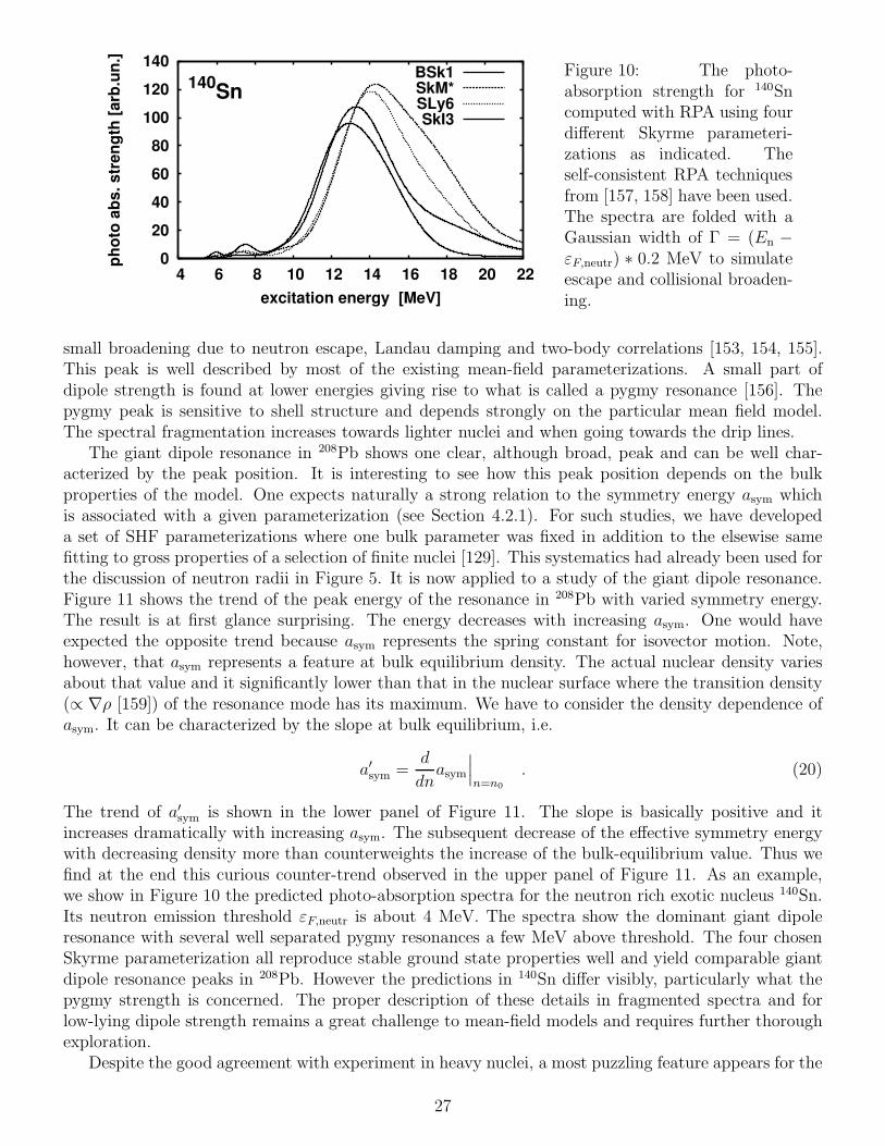
0

20

40

60

80

100

120

140

4 6 8 10 12 14 16 18 20 22

ph

oto

ab

s.

str

en

gth

[arb

.un

.]

excitation energy [MeV]

140Sn

BSk1SkM*SLy6SkI3

Figure 10: The photo-absorption strength for 140Sncomputed with RPA using fourdifferent Skyrme parameteri-zations as indicated. Theself-consistent RPA techniquesfrom [157, 158] have been used.The spectra are folded with aGaussian width of Γ = (En −εF,neutr) ∗ 0.2 MeV to simulateescape and collisional broaden-ing.

small broadening due to neutron escape, Landau damping and two-body correlations [153, 154, 155].This peak is well described by most of the existing mean-field parameterizations. A small part ofdipole strength is found at lower energies giving rise to what is called a pygmy resonance [156]. Thepygmy peak is sensitive to shell structure and depends strongly on the particular mean field model.The spectral fragmentation increases towards lighter nuclei and when going towards the drip lines.

The giant dipole resonance in 208Pb shows one clear, although broad, peak and can be well char-acterized by the peak position. It is interesting to see how this peak position depends on the bulkproperties of the model. One expects naturally a strong relation to the symmetry energy asym whichis associated with a given parameterization (see Section 4.2.1). For such studies, we have developeda set of SHF parameterizations where one bulk parameter was fixed in addition to the elsewise samefitting to gross properties of a selection of finite nuclei [129]. This systematics had already been used forthe discussion of neutron radii in Figure 5. It is now applied to a study of the giant dipole resonance.Figure 11 shows the trend of the peak energy of the resonance in 208Pb with varied symmetry energy.The result is at first glance surprising. The energy decreases with increasing asym. One would haveexpected the opposite trend because asym represents the spring constant for isovector motion. Note,however, that asym represents a feature at bulk equilibrium density. The actual nuclear density variesabout that value and it significantly lower than that in the nuclear surface where the transition density(∝ ∇ρ [159]) of the resonance mode has its maximum. We have to consider the density dependence ofasym. It can be characterized by the slope at bulk equilibrium, i.e.

a′sym =

d

dnasym

∣

∣

∣

n=n0

. (20)

The trend of a′sym is shown in the lower panel of Figure 11. The slope is basically positive and it

increases dramatically with increasing asym. The subsequent decrease of the effective symmetry energywith decreasing density more than counterweights the increase of the bulk-equilibrium value. Thus wefind at the end this curious counter-trend observed in the upper panel of Figure 11. As an example,we show in Figure 10 the predicted photo-absorption spectra for the neutron rich exotic nucleus 140Sn.Its neutron emission threshold εF,neutr is about 4 MeV. The spectra show the dominant giant dipoleresonance with several well separated pygmy resonances a few MeV above threshold. The four chosenSkyrme parameterization all reproduce stable ground state properties well and yield comparable giantdipole resonance peaks in 208Pb. However the predictions in 140Sn differ visibly, particularly what thepygmy strength is concerned. The proper description of these details in fragmented spectra and forlow-lying dipole strength remains a great challenge to mean-field models and requires further thoroughexploration.

Despite the good agreement with experiment in heavy nuclei, a most puzzling feature appears for the

27

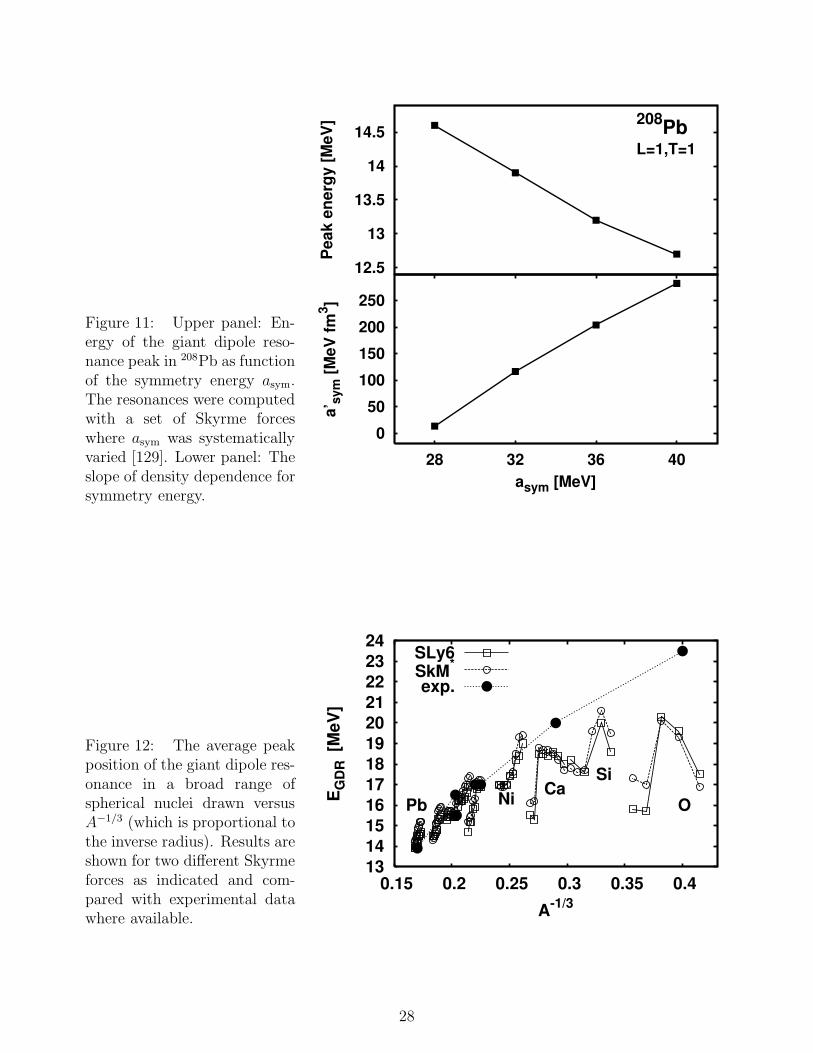
Figure 11: Upper panel: En-ergy of the giant dipole reso-nance peak in 208Pb as functionof the symmetry energy asym.The resonances were computedwith a set of Skyrme forceswhere asym was systematicallyvaried [129]. Lower panel: Theslope of density dependence forsymmetry energy.

0

50

100

150

200

250

40363228

a’ s

ym

[M

eV

fm

3]

asym [MeV]

12.5

13

13.5

14

14.5

Peak e

nerg

y [

MeV

] 208Pb

L=1,T=1

Figure 12: The average peakposition of the giant dipole res-onance in a broad range ofspherical nuclei drawn versusA−1/3 (which is proportional tothe inverse radius). Results areshown for two different Skyrmeforces as indicated and com-pared with experimental datawhere available.

13

14

15

16

17

18

19

20

21

22

23

24

0.15 0.2 0.25 0.3 0.35 0.4

EG

DR

[M

eV

]

A-1/3

OPb

SiCa

Ni

SLy6SkM

*

exp.

28

average peak position in the giant resonance region on moving to light nuclei. The average resonanceenergy is underestimated dramatically and systematically for light nuclei, such as e.g. 16O and as yet noSHF parameterization can describe adequately the resonance both in 208Pb and 16O [129]. As a first steptowards an understanding of this problem, we illustrate in Fig. 12 the trend of the average resonancefrequency over a broad range of nuclei from 16O to 208Pb. Results for two conventional SHF forces,typical for any other force investigated so far, are shown. They are drawn versus A−1/3 which helpsto spot trends. The Goldhaber-Teller model predicts an A−1/3 law while the Steinwedel-Jensen modelindicates an A−1/6 dependence [160] while experiment is closer to the A−1/6 low. The SHF theoreticalpredictions deviate from both these estimates and find a constant resonance energy for the light nuclei(large A−1/3). The clear deviation for Z < 28 nuclei is presently unexplained, thus SHF predictions canonly be considered acceptable for Z ≥ 28.

So far, we have discussed the spectra of small-amplitude modes. The lowest excitations in nucleiare often related to large amplitudes, e.g. rotations and soft quadrupole vibrations. Time-dependentmean-field theory is also capable to describe these large amplitude modes. The case of heavy-ioncollisions is discussed in the now following Section. Low-energy spectra require some additional stepsfor proper re-quantization of the semi-classical mean-field dynamics. This will be discussed in Section3.4, particularly in the part 3.4.3.

3.2.2 Gamow-Teller resonances

Giant resonances (see Section 3.2.1) and low-energy quadrupole modes (see Section 3.4.3) access mainlythe flow part of the time-odd functional in subequation (11c) of the Skyrme functional. This part isbasically fixed by Galileian invariance. Excitations with unnatural parity (Π = (−1)L+1) probe theother time-odd parts in subequation (11d) which are not yet so well fixed. Thus unnatural parity statescarry a lot of new information. In this family, the dominant isoscalar excitations have magnetic dipole(M1) structure. Orbital M1 strength is related to the nuclear scissors mode which has been observed by[161], see [162] for a review. The most prominent isovector mode is the Gamow-Teller (GT) resonance,for a review see [163]. The spectrum in the GT channel plays a role in computing the probabilities forβ-decay which, in turn, is a crucial ingredient in the reaction chains of the r-process. Furthermore, theenergy distribution of GT strength is a vital information needed for calculation of electron capture ratesat densities and temperatures appropriate for core-collapse supernovae models. Existing shell modelcalculations ([164, 165] and references therein) are not applicable for all needed neutron-heavy nucleiand extrapolation techniques have to be applied. Self-consistent SHF models are not subject to thislimitation and may prove to be a versatile tool in this context. Thus a proper modeling of these modesis a desirable feature in a self-consistent description.

While many time-odd terms contribute to isoscalar M1 excitations, GT excitations are determinedexclusively by the time-odd isovector spin-spin part of the effective interaction, see the terms ∝ C ′

0, C′2

in eq. (11d). These terms are only loosely fixed in usual parameterizations at present. Studies ofGT resonances may supply useful data for the further development of the forces. Fully self-consistentcalculations in the SHF framework are still rare, for a thorough discussion of previous work see [166].The volume properties of the residual interaction in the GT channel are characterized by the Landauparameter g′

0 [38]. The lack of predictive power becomes obvious from the fact that different SHFparameterizations shows a large spread just for this parameter. The g′

0 becomes, e.g., for the presentselection of forces: SkM*↔ 0.31, SkP↔ 0.06, SLy6↔ −0.04, SkI3↔ 0.20, SkI4↔ 1.38, BSk1↔ 0.22.Note that negative Landau parameters signify an instability of the ground state, for g′

0 a spin-isospininstability. It is to be reminded, however, that the volume parameters serve only as a first guidance.The actual situation in finite nuclei is additionally much influenced by the surface terms, in the GTchannel then by the C ′

2 term in eq. (11d). There exist already a few attempts to look for more suitableforces. The force SGII has been tailored for this particular purpose [167] and a Skyrme force SkO’

29

was found to perform fairly well in the GT channel [168]. Large scale systematic studies and a properadjustment of these features are necessary and have still to come. There exist also recent studies ofGT states within the RMF, see e.g. [169]. The advantage is here that RMF has less uncertainties inthe spin channel. It seems, however, that the modeling of the density-dependent couplings leave somefreedom yet to be fixed.

3.2.3 Heavy ion collisions

As mentioned above, fully fledged TDHF with Skyrme forces helped a lot to eludicate the principlesof heavy-ion collisions [146, 147]. It gave information on basic properties such as as the bifurcationbetween fusion and inelastic scattering at a certain critical impact parameter and the typical patternof a Wilczynski plot (double differential cross section with respect to scattering angle and energy). Theearly studies were all hampered by restrictions and approximations due to numerical limitations. One ofthe open problems was that too little dissipation emerged from these calculations thus underestimatingfusion cross sections and energy loss in inelastic collisions. A large part of dissipation could be regainedincluding the spin-orbit force properly [170, 171]. Explicit dissipation mechanisms through dynamictwo-body correlations beyond mean-field have been intensively investigated, as reviewed in [172]. Butthe full degrees of freedom of a pure TDHF description had not been explored so far. Only recentlyhas ever-increasing computing power allowed fully fledged TDHF calculations without compromises tobe explored. Glimpses of a new generation of TDHF studies are emerging, offering in assessing moreprecisely the borderline between mean field and correlation effects. [155, 173].

3.2.4 Rotational bands

Nuclear spectra exhibit extended rotational bands which disclose a variety of interesting phenomena,such as the breakdown of pairing due to the coriolis force, or the phenomenon of backbending causedby the crossing of two rotational bands with very different moment of inertia. It is no surprise then thatone can find a large body of literature on that topic, for some experimental reviews see [174, 175, 176].

Rotation is a large amplitude motion for which TDHF is the appropriate tool. However, rotationalsymmetry allows to simplification of the treatment. A transformation from the intrinsic to the labo-ratory frame shows that the rotating wavefunction is correctly described by constrained Hartree-Fock(CHF) calculation in which the mean-field Hamiltonian h is augmented by a constraint for each angularmomentum Ji, i.e.

h ←→ h− ωiJi (21)

where ωi is the Lagrange parameter (corresponding to the associated rotational frequency) and Ji isa component of the total angular momentum orthogonal to one of the principle axes of the deformednucleus. One considers usually axially symmetric nuclei and the rotation axis has then to be chosenorthogonal to the symmetry axis. This then yields unavoidably a fully triaxial problem. Moreover,time-reversal symmetry is broken by the rotation which complicates the treatment of pairing. Althoughconceptually straightforward, the technical side of these CHF calculations for rotational bands is ex-tremely involved, for details see e.g. [38]. Nonetheless, the high interest in rotational dynamics hasmotivated several groups to admirable efforts in that direction leading subsequently to the large bodyliterature as mentioned above. A detailed report would go far beyond the limits of the present review.

Mean-field theories are well suited to deal with that phenomenon since the high quantum numberinvolved validate the semi-classical limit which is implied in TDHF and self-consistency eliminates theneed for further free parameters. SHF was employed in early studies on rotating nuclei, see e.g. [177],and since then a widespread literature about rotational bands on the grounds of mean-field models,mainly SHF emerged, for reviews see e.g. [178, 179]. As discussed above, the Skyrme functional issomewhat uncertain in the time-odd domain, particularly concerning the spin couplings. This carries

30

over to the rotation studies, because rotation breaks time-reversal symmetry and thus accesses thetime-odd components of a model. The RMF method, is thought to be better suited to analyzing spinproperties since they are automatically included within the lower components of the Dirac wavefunc-tions, has been used also, however the computations are much more involved than in SHF, see forexample [180].

3.3 Nucleosynthesis

It is the present understanding that all elements in nature, apart from 1H, 2H, 3He, 4He and 7Li whichoriginated from the Big Bang [181], are made during stellar evolution and stellar explosions. The maininfluence of nuclear physics on element synthesis is given in calculation and predictions of cross sectionsof nuclear reactions and decay rates in the stellar environment. This environment is not stable butchanges on a timescale much longer than the typical time scale of the strong and week interactions,dominating nuclear transmutation. The environment, characterized by density, temperature and prop-erties of nuclei present in the medium is crucial for type, rate and products of nucleosynthesis. ThisSection reviews the role of the Skyrme interaction in simulations of the two major ways of creation ofheavy elements, the r- and rp- processes.

3.3.1 The r-process

Very neutron rich environments at high temperature permit neutron captures, much faster than compet-ing β-decay, to occur up to the neutron drip-line and are sites of the rapid neutron capture (r-process)which is thought to be responsible for creating about half of all nuclei with A≥70. Observational dataon elemental and isotopic solar abundances of nuclei (see [182] and references therein) serve as a strin-gent test of the r-process models concerning both the characteristics of the stellar environment andthe nuclear physics input. Details of the r-process models are beyond the scope of this review and aregiven elsewhere [182, 119, 181]. Here we only point out that the current understanding is that in thehigh temperature and high density environment, leading to the r-process, chemical equilibrium betweenneutron capture and the reverse photodisintegration develops within each isotopic chain (for a givenZ) and the flow along the r-process path is governed by β-decay from one isotopic chain to another. Itfollows that in equilibrium conditions the r-process path is uniquely determined by the neutron numberdensity nn, temperature T and neutron separation energy Sn(nn, T ) (Q-value) [119] and cross sectionsof individual capture processes are not important. The process is slowed down when it reaches nucleiwith magic number of neutrons (N=50, 82 and 126) and β-decay becomes comparable or faster thanneutron capture. Then a series of β-decays and (n,γ) processes takes place each changing Z and A byone [183]. The nuclei in this series are called the waiting point nuclei. As these nuclei approach stabil-ity, β-decay lifetimes get longer and the process gradually breaks off and proceeds with more favoredneutron capture (competing at some cases with β-delayed neutron emission) towards the next neutronclosed shell.

The nuclear masses (in particular neutron separation energies Sn) and gross β-decay properties(half-lives and β-delayed neutron emission probabilities) along the contour line of constant Sn arethe key nuclear inputs into r-process modeling. Another important piece of information comes frominvestigations of shell structure far from stability, in particular the strength of shell gaps which affectr-process abundances in the vicinity of magic numbers. At the endpoint of the r-process path whenfissionable nuclei are reached, β-delayed fission becomes important. The fission fragments may alterheavy element abundances and also increase general r-process abundances [181]. The important nuclearphysics input to modeling of this final phase of the r-process includes fission probabilities of nuclei athighly excited states and precise calculation of fission barriers.

Calculation of nuclear masses has been of major interest for decades. The major contribution to this

31

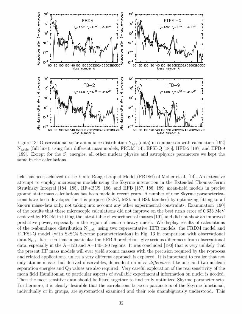
Figure 13: Observational solar abundance distribution Nr,⊙ (dots) in comparison with calculation [192]Nr,calc (full line), using four different mass models, FRDM [14], EFSI-Q [185], HFB-2 [187] and HFB-9[189]. Except for the Sn energies, all other nuclear physics and astrophysics parameters we kept thesame in the calculations.

field has been achieved in the Finite Range Droplet Model (FRDM) of Moller et al. [14]. An extensiveattempt to employ microscopic models using the Skyrme interaction in the Extended Thomas-FermiStrutinsky Integral [184, 185], HF+BCS [186] and HFB [187, 188, 189] mean-field models in preciseground state mass calculations has been made in recent years. A number of new Skyrme parameteriza-tions have been developed for this purpose (SkSC, MSk and BSk families) by optimizing fitting to allknown mass-data only, not taking into account any other experimental constraints. Examination [190]of the results that these microscopic calculations did not improve on the best r.m.s error of 0.633 MeVachieved by FRDM in fitting the latest table of experimental masses [191] and did not show an improvedpredictive power, especially in the region of neutron-heavy nuclei. We display results of calculationsof the r-abundance distribution Nr,calc using two representative HFB models, the FRDM model andETFSI-Q model (with SkSC4 Skyrme parameterization) in Fig. 13 in comparison with observationaldata Nr,⊙. It is seen that in particular the HFB-9 predictions give serious differences from observationaldata, especially in the A=120 and A=140-180 regions. It was concluded [190] that is very unlikely thatthe present HF mass models will ever yield atomic masses with the precision required by the r-processand related applications, unless a very different approach is explored. It is important to realize that notonly atomic masses but derived observables, dependent on mass differences, like one- and two-nucleonseparation energies and Qβ values are also required. Very careful exploration of the real sensitivity of themean field Hamiltonian to particular aspects of available experimental information on nuclei is needed.Then the most sensitive data should be fitted together to find truly optimized Skyrme parameter sets.Furthermore, it is clearly desirable that the correlations between parameters of the Skyrme functional,individually or in groups, are systematical examined and their role unambiguously understood. This

32

may provide a very powerful and decisive constraint in the search for meaningful Skyrme functionals.

Gross β-decay properties have been treated in a variety of models (see, e.g. [193]) that range fromphenomenological to large scale microscopic calculations. At this point all models have some deficiencyand it is not yet possible to calculate the whole r-process. The limitations are mainly in restrictionto spherical shapes, Gamow-Teller (GT)-transitions only, or too small shell model spaces. One of thekey issues is as-correct-as-possible treatment of nucleon-nucleon correlations in a model. The only fullyself-consistent HFB+QRPA calculation of β decay rates of the r-process waiting-point nuclei utilizedthe Skyrme parameterization SkO′ [194]. An important extension of the Skyrme-HFB model employedhere was the incorporation of time-odd terms in the Hamiltonian, needed for the correct treatment ofthe GT excitation. These terms contribute to the energy of polarized states, i.e. those with non-zeroangular momentum, including the 1+ states populated in the β-decay. They are usually neglectedin Skyrme-HF calculations which are then strictly speaking applicable only to even-even nuclei. Theconsequence of consideration of the T-odd terms is the introduction of additional variable parametersand their relationship with the parameters of the T-even part of the Hamiltonian has to be established[195]. The results of this calculation include a study of the GT-strength distribution over the spectrumof excited states and the effect of the strength of the pn particle-particle interaction. It was shownthat the HBF-QRPA model [194] in all but very heavy nuclei calculates half-lives that are shorter thenpredictions of the FRDM+QRPA [196] and EFTSI+QRPA [197] in some cases in improved agreementwith experiment. Unfortunately, a full study of the impact of the calculation on the r-process couldnot be completed because not all waiting point nuclei were calculated and the no deformation effectswere included in the model. It would be desirable to follow up this issue and establish the origin of thedifference in predictions of β-decay half-lives.

The presence and strength of neutron shell closures affects the rate of the r-process flow throughthe waiting point nuclei. This information comes from mean field or other mass model calculationsand, to large extent, from experiment (see e.g. [193] and references therein). It has been shown [198]that, for example, abundance deficiencies around A=120 and A=140, calculated using mass predictionsfrom global macroscopic-microscopic models, indicated too strong N=82 shell closure. When the masseswere calculated locally in the vicinity of the shell closure using an HFB model with SkP force whichpredicted quenching of the N=82 gap, the agreement between calculated and observed solar r-processabundances seriously improved. At the present time it is clear that existence of yet unknown changesin the shell structure at the neutron drip-line region may have a profound impact on the flow of ther-process.

3.3.2 The rp-process

Hot environments with a large surplus of hydrogen (protons) permit proton capture on seed nuclei closeto the stability line up to proton drip-line - in a process called the rapid proton capture (rp-process)[199]. It originates in explosive hydrogen burning at temperatures high enough that a break-out ofthe hot CNO cycle is possible. It proceeds by a series of proton capture reactions and β+-decays andat sufficiently high density and temperature can get well beyond A=64 and Z=32 [200] until the rp-process reaches the proton drip line. The rp-process is thought to be the dominant source of type IX-ray bursts and responsible for the nuclear composition of the crust of an accreting neutron star [201].The key nuclear input includes proton separation energies Sp to determine proton capture and reversephotodisintegration, alpha separation energies Sα for treatment of back-processing via α emission or(γ, α) disintegration and Qβ+ = QEC - 2mec

2 for calculation of the rate of weak processes along therp-process path.

As for the r-process, the lack of experimental data in important regions of the rp-process path forcesus to turn to theoretical models. The mass models play, as usual, a key role. Weak interaction ratesare usually known experimentally for nuclei with Z ≤ 34. For β-decay of isotopes heavier than A = 20

33

the decay from thermally populated excited states has to be taken into account and the temperaturedependence of the decay rate has to be calculated. The standard approach is to calculate these rateswithin QRPA [196] and, wherever possible, in the shell model.

An interesting attempt to calculate properties of nuclei along the rp-process path close to the protondrip-line has been reported by Brown et al., [202] who calculated one-proton and two-proton separationenergies in the spherical Skyrme HF model. They calculated Coulomb displacement energies of mirrornuclei and utilized known masses of the neutron rich partner of a mirror pair. The newly developedSkX Skyrme parameterization with a especially added charge symmetry breaking (CSB) term was used[203]. The results in the region of A = 41–75, given with the error dependent on the experimental errorof the neutron-rich nucleus and assumed 100 keV theoretical error, were extensively tested in rp-processsimulation and models for the x-ray burst. It has been clearly shown that the x-ray burst tails aresensitive to nuclear masses at and beyond the N = Z line between Ni and Sr. The new calculationleads to a tighter constraint on proton capture Q values as compared to extrapolation of experimentalmasses [191]. The authors connect this success with the special parameterization of the SkXCBS forceto account for charge-symmetry breaking. The results are indeed better in comparison with the originalSkX force. However the question remains how unique is this extension of the SkX force and, whethersome other parameterizations than SkX would behave similarly if the CSB term was added to them.

3.4 Beyond the mean-field: Collective correlations

3.4.1 Large amplitude collective motion

As outlined in Section 2.1.1, correlations cover anything beyond mean field and embrace very differentmechanisms. Short-range and long-range correlations are assumed to be incorporated into the effectiveenergy-density functional. Collective correlations, however, cannot be accounted for in a simple energy-density functional and need to be considered as explicit correlations in addition to the mean fieldcalculations.

The effective energy functionals can still be used for that task since low-energy (and thus largeamplitude) collective motion can be derived as the adiabatic limit of time-dependent mean fields. Thisapplies exactly to center of mass motion which perfectly decouples from internal excitations but to agood approximation also. This applies to rotation whose ground state has zero energy and where theexcitation energies are by far the smallest in the nuclear spectrum. The approach has been usuallyapplied to low-energy modes associated with surface vibrations of quadrupole type, sometimes also ofoctupole nature. The zero-energy modes (center of mass in Section 2.2.3, rotation in Section 3.2.4)are related to symmetry breaking through the mean field and restoration through correlations. In thesame spirit, this includes also particle-number projection in connection with BCS states although theassociated collective ‘deformation’ corresponds to a motion through phase angles and does not have anygeometrical interpretation.

Somewhat in analogy to the Born-Oppenheimer picture in molecular physics, the adiabatic motionis thought to evolve along a collective path which is set of mean-field states |Φq〉 where q labelsthe collective deformation (e.g., rotation angle or quadrupole momentum). In the ideal case, the pathis generated by adiabatic TDHF (ATDHF) [204, 205, 39]. In practice, one approximates that by aconstrained Hartree-Fock (CHF) calculation in which a wanted deformation q = 〈Φq|Q|Φq〉 is achieved

by adding a constraining operator to the mean field Hamiltonian, i.e. h −→ h − λQ where λ is theLagrange multiplier. The dynamical properties are explored by self-consistent cranking taken overfrom the ATDHF scheme. The collective spectrum (correlated ground state and excitations) is usuallydescribed within generator-coordinate method (GCM) as a coherent superposition of these deformedmean-field states i.e.

|Ψn〉 =

∫

dq |Φq〉fn(q) . (22)

34

4

6

8

10

12

14

60 65 70 75 80 85

δ 2p

[MeV

]

Neutron Number N

Z=50

SkI3

spherical MFdeformed MF

mf + GSCExp.

Figure 14: The two-protonshell gap δ2p calculated forthe interaction SkI3 at variouslevels of the model: sphericalmean field, deformed meanfield, and with collectiveground state correlations fromquadrupole vibration androtation. The experimentaldata are taken from [209].

The equations for the superposition functions fn(q) are obtained by variation. The machinery of theGCM and the various approximations invoked in actual calculations are a large topic, far beyond thescope of this review. We refer to summaries in [39, 206, 38, 22] and mention only the two basicallydifferent solution schemes: some groups go for a direct numerical attack on a finite grid of |Φq〉, othergroups deduce a collective Hamiltonian in terms of the q and solve that.

The deformation coordinates q embrace all the typical low energy modes. The three nuclear center ofmass coordinates are included among these and their approximate treatment leads to the c.m. correctionas explicitely included in the energy functional and as discussed in Section 2.2.3. The next importantconsiderations are the five coordinates for vibration-rotation, either as the five quadrupole momentaor recoupled to total quadrupole coordinate β, triaxiality γ, and three Euler angles [207]). The GCM,or collective Hamiltonian, in these coordinates yields the low-energy quadrupole spectra and consistentwith it also the correlated ground state associated with the lowest solution f0. An example of spectrawill be discussed in Section 3.4.3 and of ground-state correlations in 3.4.2. It is to be noted that octupolemodes can also become very soft and accessible to the adiabatic picture, for a typical application seee.g. [208].

What is meant by ‘beyond mean field’ clarifies when we consider in GCM ansatz (22) expressedsums of mean field states. The superposition is necessary for a fully quantum mechanical treatmentof the system. TDHF as such can also describe large amplitude motion and it does it in terms of atrajectory |Φ(t)〉 which remains at every instant a mean-field state and never goes ‘beyond’. One cansay that TDHF represents the classical limit of many-body dynamics. The classical trajectory belongsto the mean-field approach and GCM serves to ‘re-quantize’ the description. There are regimes ofcollective motion where a semi-classical description suffices, such as fission which had been discussed inSection 3.1.5 and heavy-ion reaction which were sketched in Section 3.2.3. A particularly subtle caseare the small amplitude vibrations discussed in Section 3.2.1 and 3.2.2. TDHF allows computation ofthe frequency spectrum of classical vibrations. The re-quantization is performed unconsciously throughthe equivalence of classical and quantum-mechanical picture for the harmonic oscillator. That simpleequivalence fails for non-harmonic motion which is usually encountered in soft modes and this, in turn,requires the elaborate GCM techniques.

35

3.4.2 Correlations from soft modes

The impact of collective correlations on bulk properties of semi-magic nuclei is generally very small.That is why these nuclei are preferable used in the fitting of forces. The situation may change, however,when considering the much more sensitive isotopic or isotonic differences. The crucial influence ofcollective correlations on isotopic differences of radii, the isotopic shifts [210], has been long recognizedin many places, e.g. [211, 212]. The effect on energy differences, though less in focus up to now, is notless important. As an example, Figure 14 shows the second energy difference, the two-proton shell gap,

δ2p = E(Z+2, N)− 2E(Z, N) + E(Z−2, N), (23)

in Sn isotopes. The results from all spherical calculations agree very nicely with twice the spectral gapat the magic Z = 50 shell closure. This confirms the idea behind using the shell gap as a measureof the spectral gap. However, the spherical results are far from the measured values, in both size andtrend. As a next step, we allow for (axially) deformed ground states. This lowers the δ2p gap for theisotopes with low neutron number because the neighboring isotones (Cd and Te) gain binding energythrough deformation while semi-magic Sn remains spherical. The deformation effect is still insufficientto match experimental gaps. We are obviously in a transitional regime between spherical and deformedshapes where we expect large shape fluctuations and consequently substantial collective correlations.And indeed, the δ2p gaps obtained using correlated ground states match experimental values verynicely. (These calculations were done within the Gaussian Overlap Approximation to GCM, for detailssee [213].) This example shows that correlation can have a dramatic effect on isotopic (or isotonic)differences. It need not always be that dramatic – a similar study in the Pb isotopes has shown thatthere the deformation effect suffices to reproduce the data [214]. Nonetheless, a careful check is advisablein any case.

3.4.3 Low energy quadrupole excited states

There is a widespread literature on the computation of low-energy spectra on the basis of SHF or theGogny model using various variants of the GCM. These deal mainly with low-lying quadrupole excitedstates, see e.g. [215, 216, 217], sometimes also octupole excitations, see e.g. [208, 218]. Well adjustedmodern Skyrme parameterizations provide usually a pertinent description of these soft modes. Theirtypical performance is demonstrated in Figure 15 taking Sn isotopes as example. Doubly magic 132Snis clearly distinguished by its large excitation energy. Pairing is inactive in a doubly-close-shell nucleusand the energy spectrum is closely related to shell structure, in particular the shell gap in the single-nucleon spectra. The low lying quadrupole mode in all other isotopes is dominated by the pairing gap.It is no surprise then that many different SHF parameterizations yield very similar results providedthat the pairing strength has been calibrated properly for each case. The crucial influence of pairing isdemonstrated for SkI3 by reduction of the pairing strength by to 75% of the standard strength. Theparticularly strong effect seen around neutron number N = 68 is related to a semi-shell closure at apoint at which the BCS scheme runs into a critical regime close to breakdown.

As discussed above, the results for the excitation energy are generally very satisfying. The transitionmoments, however, are not yet so well described as is true of most models. This is because the momentsare much more sensitive to the collective mass which, in turn, is extremely sensitive to the choice ofthe collective path [219]. We suspect that moment calculations could be much improved by using thefull ATDHF instead of approximating it through CHF. In spite of this unresolved detail, we want toemphasize that self-consistent mean-field models with well adjusted bulk and pairing properties yielddirectly a pertinent description of large amplitude collective dynamics without thee need of additionalre-tuning.

36

0

1

2

3

4

5

E(2

+)

(Me

V)

SkI3SkI3, red.gap

SLy6exp.

0.8

0.6

0.4

0.2

0 66 70 74 78 82 86 90

B(E

2)↑

(e

2 b

2)

Neutrons

Figure 15: The energy (upperpanel) and B(E2) transitionmoments (lower panel) of thelowest quadrupole state (2+)in Sn isotopes computed withtwo different forces as indicatedand compares with experimen-tal data. For the force SkI3, wealso consider the case of a 75%reduced pairing strength.

4 Infinite matter and astrophysical applications

The concept of infinite nuclear matter has been introduced to nuclear physics as an extrapolation of thealmost homogenous conditions in the center of heavy nuclei. In this fully homogeneous matter the dif-ference between neutrons and protons is neglected and no single particle effects are considered. Theseconditions lead to constant density and the absence of Coulomb energy, pairing and surface effects.These features make it an attractive medium for testing and comparing models of bulk nuclear proper-ties. Infinite nuclear matter is, however, not an observable system and the quantities characterizing itsproperties are of empirical nature (see Section 4.2.1). There are two limiting states of infinite nuclearmatter, symmetric nuclear matter (SNM) with equal number of protons and neutrons and pure neutronmatter (PNM) with no protons present. These two states have fundamentally different properties. Theenergy per particle in SNM reaches a negative minimum value (i.e. it saturates) at a saturation density

n0

(=0.16 fm−3), corresponding to the lowest bound state of SNM (the ground state). On the contrary,the energy per particle in PNM is predicted to be always positive, i.e. PNM as such does not exist in abound state and represents the highest excited state on nuclear matter. These properties of SNM andPNM place powerful constraints on the parameters of the Skyrme interaction, as will be discussed later.

Asymmetric nuclear matter that lies between the two extremes with the proton/neutron ratio be-tween zero and one has become a popular medium for modeling large fractions of stellar matter incompact objects, in particular in cold neutron stars. Note that the term ‘compact object’ in astro-physics refers to an object whose gravity produces a deep potential well. It is most commonly used todescribe neutron stars and black holes but is sometimes also used to refer to white dwarfs. Note thatthe defining feature is the depth of the potential well and not the strength of gravitational forces (whichcan be quite modest in the case of high-mass black holes). The deep potential well means that lightcoming from the surface to an outside observer is significantly redshifted and light rays passing closeto the object are significantly bent. The equation of state of nuclear matter is constructed from thecalculated density and composition dependence of energy per particle, as discussed in Section 4.2. There

37

is no direct experimental information available on the behavior of the energy per particle in nuclearmatter. Theoretically it exhibits strong dependence on the properties of the interaction between parti-cles present in the matter. In the investigation of this dependence for different parameterizations of theSkyrme interaction, we use as a benchmark the ab-initio calculation with the realistic A18+δv+UIX∗

(APR) potential [220]. The APR model is based on the Argonne A18 two-body interaction and in-cludes three-body effects through the Urbana UIX∗ potential and boost corrections to the two-nucleoninteraction which gives leading relativistic effects of order (v/c)2. This interaction is considered as oneof the most modern realistic potential used for description of nuclear matter at present.

4.1 Relevance of nuclear properties to physics of compact objects

In order to construct compact star models, it is necessary to have an equation of state (EoS) linkingpressure with total energy-density and, to obtain this, expressions must be supplied for the interactionpotentials or energy functionals of the particles concerned [221, 222, 223]. The basic ingredient ofthe EoS, the effective nucleon-nucleon interaction, is not very well known and assumptions need tobe made about its nature and form, particularly as regards its behavior as a function of density. Inthis section we concentrate on the role the non-relativistic phenomenological Skyrme interaction playsin this context, and its limitations. Especially relevant for our discussion are cold, non-rotationalneutron stars as naturally occurring compact objects. At around nuclear matter density, neutron starmatter can be well-represented as a homogeneous mixture of neutrons, protons, electrons and muons(n+p+e+µ matter) representing beta-equilibrium matter (BEM). These densities turn out to be crucialfor determining the properties of neutron star models with masses near to the widely-used ‘canonical’value of 1.4 M⊙. However, models of non-equilibrium systems like core-collapse supernovae, both atsub- and super- nuclear densities, also use EoS based on the Skyrme interaction [224].

We focus here on to what extent SHF fulfills the important requirement that it describes not onlyfinite nuclei but is also valid in infinite nuclear matter. Almost 90 Skyrme functionals were recentlytested in nuclear matter and cold (T=0) non-rotational neutron star models. Details can be found in[28]. Here we state only the main conclusion drawn in [28] that Skyrme interactions, giving broadlysimilar agreement with the experimental observables of nuclear ground states as well as with propertiesof SNM at saturation density, predict widely varying behavior for the observables of both symmetricand asymmetric nuclear matter as a function of particle number density. The underlying property,decisive for the validity of a Skyrme interaction in nuclear matter models, is the density dependence ofthe symmetry energy. Here we will demonstrate this result and its implications for models of neutronstars on the same set of the Skyrme parameterizations used in the previous sections, SkM∗, SLy6, SkP,SKI3, SkI4 and BSk1 as examples.

The requirement that SHF remains applicable in various astrophysical scenarios, utilizing the grow-ing amount and precision of observational data, in particular on neutron stars, places important con-straints on the optimal parameter sets. These will be discussed throughout the coming sections.

4.2 Relation to SHF and the Equation of State

The key property of a system for use in EoS models is the total energy per particle E = E/A. Asdiscussed above (see Section 4), nuclear matter is a medium of constant density. This simplifies signifi-cantly the total energy defined for finite nuclei by equation (11) in Section 2.2.2. All terms dependingon ∆ρ, j, σ, and J vanish. The assumption of absence of the Coulomb force in nuclear matter is inline with the condition for existence of stars, bound together by the gravitational force, many ordersor magnitude weaker than the electromagnetic force. The c.m. correction approaches zero in infinite

38

matter and pairing is neglected as well. Thus the Skyrme energy functional in nuclear matter becomes

E =

∫

d3 nEkin + nESkyrme , (24a)

nESkyrme =B0 + B3n

α

2n2 −

B′0 + B′

3nα

2n2 + B1nτ − B′

1nτ (24b)

where Ekin is taken in the same form as (11). The terms ∝ B0, B′0 correspond to a zero-range attractive

two-body force, terms ∝ B3, B′3 to a density-dependent repulsive force, and those ∝ B1, B

′1 are related

to the nucleon effective mass. The above expression for ESkyrme is a function of 7 variable parametersBi, B

′i and α. It is sometimes convenient to express them in terms of 9 alternative Skyrme parameters

ti, xi and α [225] using relations (12).The relation between finite nuclei and infinite matter is established by considering a finite volume

V of homogenous matter containing N neutrons and Z protons, forming A = N + Z nucleons. Formatter with N6=Z the asymmetry parameter is defined as the ratio

I =N − Z

A=

nn − np

n=

n

n. (25)

Then the proton and neutron number densities are given in terms of I and n as

np =Z

V=

n

2(1− I) , nn =

N

V=

n

2(1 + I) , n =

A

V= nn + np . (26)

Using the expression for the energy E (24a) we define the total energy density of nuclear matter

ǫ(n, I) = n(E + mc2) (27)

where E = E/A is the binding energy per particle while nE = E/V is the energy density, i.e. the energyper volume.

Nuclear matter obeys the standard thermodynamical relation between pressure P and Helmholtzfree energy F = E − TS where E is the internal energy (24a) and S is the entropy, namely

P =∂F

∂V

∣

∣

∣

T,S. (28)

This can be rewritten in terms of n and I in the form

P = n2 ∂F(n, I)

∂n

∣

∣

∣

T,I, F =

F

N. (29)

where F is the free energy per particle. For systems at zero temperature (T = 0) the equation (29)reduces to

P = n2 ∂E(n, I)

∂n

∣

∣

∣

I. (30)

The pressure is fully determined by the total energy per particle E(n, I) and its dependence on theparticle number density n and composition I. This relation is often called the equation of state forconvenience - it can be very easily converted to the more customary form relating pressure, temperatureand volume as demonstrated above. We illustrate, in Figure 16, the energy per particle E as a functionof total nucleon number density n for six different parameterizations of the Skyrme interaction discussedabove in Section 3. The calculation has been performed at zero temperature for the two extreme phasesof nuclear matter, SNM at I = 0 and PNM at I = 1. Examination of Figure 16 shows that the densitydependence of E for SNM is calculated to be rather similar for all the selected parameterizations andcompares reasonably well with values yielded by the APR model. However this general agreement doesnot carry over to the predictions for PNM for which the density dependence of E varies significantlyfor different SHF parameterizations at densities higher than about 0.2 fm−3 and agrees with the APRresult only for SLy6.

39

0

100

200

300

En

erg

y p

er p

arti

cle

[MeV

]

SNM SkM*

PNMSNM APRPNM

SNM SkPPNM SNM APRPNM

SNM SLy6PNMSNM APRPNM

0 0.2 0.4 0.6 0.8 1

n [fm-3

]

0

100

200

300

En

erg

y p

er p

arti

cle

[MeV

]

0

0

100

200

300

SNM SkI3PNMSNM APRPNM

0 0.2 0.4 0.6 0.8 1

n [fm-3

]

SNM SkI4PNMSNM APRPNM

0 0.2 0.4 0.6 0.8 1

n [fm-3

]

SNM BSk1PNMSNM APRPNM

Figure 16: The energy per particle for SNM and PNM is plotted as a function of baryon number densityn for SkM∗, SkP, SLy6, SkI3, SkI4 and BSk1 Skyrme parameterizations. For comparison, also shownare equivalent curves for SNM (triangles) and PNM (circles) calculated using the APR potential [220].For more explanations, see text.

40

4.2.1 Key properties of nuclear matter

Although infinite nuclear matter is not directly observable, the equilibrium parameters of SNM andsome properties of asymmetric matter provide a physically plausible and intuitive way to characterizethe bulk properties of a model. We consider in the following paragraphs the saturation density ofnuclear matter n0, the binding energy of SNM E at this density, the incompressibility modulus K, thesymmetry energy asym and the isoscalar and isovector effective nucleon masses. Currently acceptedvalues are then compared with predictions of the selected Skyrme parameterizations and with selectedinteraction used in RMF models discussed in Section 2

The energy functional provides the binding as function of the isoscalar and isovector densities, i.e.E(n, n). In SNM, the equilibrium energy and density are defined by the condition

∂E

∂n= 0 (31)

(the other condition ∂E/∂n = 0 is automatically satisfied for n = np−nn = 0). The best estimate of thedensity n0 of symmetric nuclear matter at saturation is based on the comparison of experimental andcalculated charge distribution in heavy nuclei. The most precise value n0 = 0.16± 0.005 fm−3 is givenin [225]. A more conservative value of 0.17±0.02 fm−3 is given in Ref.[226] where the error bar includesuncertainties in the neutron density distribution and a correction for possible density inhomogeneity innuclear interior. The value of 0.16± 0.02 fm−3 quoted in [221] is of the same precision as that in Ref.[226].

The accepted value of E0 = E(n0, I = 0) at saturation (i.e. the minimum value) is taken to beequal to the coefficient of the volume term av in the liquid-drop model, obtained by fitting the bindingenergies of a large number of nuclei. This procedure gives E0 = −(16.0± 0.2) MeV [225].

The incompressibility modulus K is related to the curvature of E/A as [225]

K(n) = 9n2∂2E

∂n2+ 18

P (n)

n. (32)

The value of K∞ = K(n0) at saturation (P = 0), represents an important constraint on models ofnuclear matter. However K∞ is a derived quantity and its ‘best’ value is model dependent. Nix andMoller estimate K∞ ≃ 240 MeV [227], while Hartree-Fock + RPA calculations of the giant isoscalarmonopole resonance (the breathing mode) [228] imply K∞ = (210±20) MeV both with the use of Skyrmeinteractions [229] and with the Gogny potential [230]. The generalized Skyrme interactions [231], fittedboth to finite nuclei and the breathing mode energies, give the best results for K∞ = (215± 15) MeV.In the non-relativistic approximation, the speed of ordinary sound in the nuclear medium is related tothe incompressibility modulus K by [221]

vs

c=

dP (n)

dǫ=

√

K(n)

9(mc2 + E + P (n)n

). (33)

It is desirable to check the density dependence of the speed of sound as it may exceed the velocity oflight at higher densities in non-relativistic models [221] and this unrealistic feature must be avoided.

One of the key properties of nuclear matter is the symmetry energy, particularly important in themodeling of nuclear matter and finite nuclei because it depends on the isospin part of the interactionand is relevant for correctly describing nuclei with high values of isospin far from stability. It reads

S(n) = E(n, I = 0)− E(n, I = 1) . (34)

This quantity is related to the asymmetry coefficient asym in the semiempirical mass formula under twoassumptions, (i) E(n, I = 0) is the minimum energy of the matter at given density n and thus in the

41

-200

-100

0

100

200

a s [M

eV]

SkM*

APR

SkPAPR

SLy6APR

0 0.2 0.4 0.6 0.8 1

n [fm-3

]

-200

-100

0

100

200

a s [M

eV]

SkI3PNM

0 0.2 0.4 0.6 0.8 1

n [fm-3

]

SkI4APR

0 0.2 0.4 0.6 0.8 1

n [fm-3

]

BSk1APR

Figure 17: The asymmetry coefficient asym as a function of particle number density n for the six Skyrmeparameterizations compared with the APR [220].

expansion of E(n,I) about this value with respect to I (or equivalently n) the leading non-zero term isthe second derivative term and (ii) all the other derivatives in the expansion are negligible. Then [96]

asym =1

2

∂2E

∂I2

∣

∣

∣

∣

I=0

=n2

2

∂2E

∂n2

∣

∣

∣

∣

n=0

. (35)

In practice, E(n,I) contains always a small component ∝ I4 [96] and thus expression (35) should betreated as approximation. A value asym = 32.5±0.5 MeV is found by fitting a large set of experimentaldata in the Finite-Range-Droplet-Model (FRDM) [232]. The extrapolation of the various fits for thenon-relativistic models (SHF and Gogny) yield typical values of asym in the region of 27-38 MeV, see[221, 186, 22, 96] and Figure 18. The various RMF parameterization yield values in the 35–42 MeVrange, see [233, 22, 96] and Figure 18.

The density variation of the asymmetry energy coefficient asym, defined by Eqs. (34) and illustratedin Figure 17 is determined by the density dependence of E in SNM and PNM. We see two distinctlydifferent patterns for the various Skyrme parameterizations; asym is either growing or decreasing withincreasing particle number density. A more detailed analysis even distinguishes between the rate ofdecrease of asym with increasing n [28]. The transition to a negative value of asym indicates that PNMbecomes the ground state (which is unphysical [234]), the pressure becomes negative and the mattercollapses. This is the case of the SkP and BSk1 parameterizations as shown in Figure 17. Another (early)indicator of a possible collapse of nuclear matter at high densities is too low a value for the derivativeof the symmetry energy with respect to particle number density at n0 (see Table 2). As we will showin the next section that such parameterizations cannot produce neutron-star models with masses ashigh as the ‘canonical’ 1.4 M⊙ and so they should be excluded from consideration for astrophysicalpurposes. Of our sample group this applies to BSk1 and SkP, but there are more examples of Skyrme

42

0.92

0.94

0.96

0.98

1

NL

-Z

NL

3

PC

-F1

SkI4

SkI3

SL

y6

BS

k1

SkP

SkM

*

n0/n

0(L

DM

)

0.92

0.94

0.96

0.98

1

(E/A

)/(E

/A)(L

DM

)

0.7

0.8

0.9

1

1.1K

nm

/K(L

DM

)

0.6

0.7

0.8

0.9

1

ms

* /m

0.9

1

1.1

1.2

1.3

NL

-Z

NL

3

PC

-F1

SkI4

SkI3

SL

y6

BS

k1

SkP

SkM

*

as

ym

/as

ym

(LD

M)

0

0.2

0.4

0.6

0.8

κ

Figure 18: The key properties of nuclear matter: n0 = saturation density of symmetric nuclear matter;E/A = binding energy per particle; Knm ≡ K∞ = incompressibility; m∗

s/m = isoscalar effective nucleonmass; asym = asymmetry coefficient; κ = isovector sum-rule enhancement factor (related to isovectoreffective mass; Results for n0, E/A , K∞, m∗

s/m and asym are shown for a variety of Skyrme and RMF

parameterizations (see Table 1) as a ratio to the corresponding LDM values [26, 236]. κ is given inabsolute units as LDM value is not available for this quantity.

parameterizations with the same behavior as SkP and BSk1 in nuclear matter, identified as ‘group III’in [28].

Finally, the isoscalar and isovector effective nucleon masses in infinite nuclear matter (denoted bym∗

s/m and m∗v/m respectively, measured in units of the vacuum nucleon mass m) can be written as

functions of the Skyrme parameters and the density of the medium. The effective neutron mass in denseasymmetric matter is then given by [235]

~2

m∗n

= (1 + I)~

2

m∗s

− I~

2

m∗v

(36)

and similarly for the effective proton mass m∗p. The isoscalar nucleon mass is deduced from the variation

∂τE of the the energy functional and the isovector effective mass comes from the variation ∂τE. Thelatter can be also formulated in terms of the isovector sum rule enhancement factor κ [38] where

m∗v

m= (1 + κ) (37)

A value of κ = 0 means no enhancement, i.e. the isovector effective mass equals the bare mass. Typicalare slightly positive κ around 0.25 although little is certain about this parameter (for details see [22]).

Figure 18 summarizes the predictions for these basic properties of SNM at saturation density result-ing from SHF with our six parameterizations and in RMF using parameterizations PC-F1, NL-3 and

43

NL-Z in comparison with predictions of the Liquid Drop Model (LDM). Binding energy and saturationdensity show little variation within the SHF forces and agree well with the LDM values. The RMFdiffers, slightly but significantly. The reasons are not yet understood. The incompressibility K∞ showslarger fluctuations, but they gather nicely around a generally accepted value of 230 MeV. The isoscalareffective mass m∗

s/m tends to values below one. It is, however, a vaguely fixed property in SHF asone can see from the large spread of results. Information on excitations is required to better constrainthe effective mass, see e.g. [237, 238] for the impact of giant resonances. The RMF always prefersparticularly low values which reflects the counteracting interplay of the rather strong scalar and vectorfields [94].

The isovector parameters asym and κ are much less well determined because of the limited extensionof isotopic chains in the nuclear landscape. There are systematic differences between SHF and RMFwith RMF predicting generally larger values. The SHF values are more consistent with the LDM whichgives them somewhat better credibility. Since the standard RMF model has much less flexibility inthe isovector channel, it is much harder to fit long isotopic sequences and, in the extreme, sometimesimpossible to produce the equation of state for pure neutron matter [239]. For that reason, extensionsof the RMF are being developed which provide more isovector flexibility [102, 103].

4.2.2 β-equilibrium matter

In cold neutron stars, as the density increases from about 0.75 n0 up to 2–3 n0, nuclear matter becomesa system of unbound neutrons, protons and electrons and muons and, if enough time is allowed, willdevelop equilibrium with respect to weak interactions. All components that are present on a timescalelonger than the life-time of the system take part in equilibrium. For example, neutrinos created in weakprocesses in a cold neutron star do not contribute to the equilibrium conditions as they escape rapidly.In this section we explore insights into the validity of the selected Skyrme parameterizations obtainedby investigating the density dependence of the properties this homogenous phase.

BEM is characterized by the following processes:

n↔ p + e− ↔ p + µ− .

Equilibrium implies that the chemical potentials should satisfy the conditions

µn = µp + µe, µµ = µe , (38)

with each chemical potential µj defined by

µj =∂ǫ

∂nj(39)

where ǫ is the total energy density (27) and the nj’s are the particle number densities. Particle fractionswith respect to the total nucleon number density n are given as:

yj =nj

n. (40)

Charge neutrality of BEM implies np = ne + nµ.The composition of BEM has significant impact on the properties of neutron stars. In particular,

the value taken by the proton fraction yp has relevance for neutron star cooling, as discussed in [240].The proton fraction is related to the asymmetry parameter I, introduced earlier, by I = 1 − 2yp andcan also be expressed in terms of the symmetry energy (34) by [221]

~c(3π2nyp)1/3 = 4S(n)(1− 2yp) . (41)

44

Table 2: Observables of nuclear matter and cold (T=0) non-rotating neutron stars: Calculated maxi-mum mass with corresponding radius and central density, and the radius and binding energy of a 1.4M⊙ star for Skyrme functionals SkM∗, SkP, SLy6, SkI3, SkI4 and BSk1. The symmetry energy at satu-ration density n0, 3n0 and the derivative of the symmetry energy at the saturation density ∂as/∂n(n0)are also given. Results for four other EoS based on different models of the nucleon-nucleon interaction,are added for comparison. See text for more explanation.

EoS as(n0) as(3n0) ∂as

∂n(n0) Mmax Rmax ncentr

max ρcentrmax R1.4M⊙

Ebin

[MeV] [MeV] [M⊙] [km] fm−3 g/cm3 [km] [1053 ergs]SkM∗ 30.01 34.02 +95 1.62 8.94 1.66 3.80 10.54 3.09SkP 29.71 -0.43 +43 0.60 814SLy6 32.09 51.84 +99 2.05 10.05 1.19 2.82 11.76 2.58SkI3 34.27 125.00 +212 2.19 11.19 0.98 2.33 13.56 2.18SkI4 29.50 98.85 +125 2.15 10.71 1.05 2.49 12.56 2.43BSk1 27.86 -15.06 +12 0.61 1089FP 31 40 1.95 9.0 1.3

APR 33.94 59.67 2.20 10.01 1.14 2.73 11.47 2.75BJ 1.85 9.90 1.31 3.06 11.86 2.51

Hybrid 1.45 10.45 1.36 2.76 11.38 2.49

An equation of state for zero-temperature beta-stable nucleon+lepton matter can be constructedfrom SHF following a procedure described previously, see e.g. [28, 225, 240]. The total energy densityof the BEM is written as the sum of the nucleon and lepton contributions[225]:

ǫ(np, nn, ne, nµ) = ǫN (np, nn) + nnmnc2 + npmpc

2 + ǫe(ne) + ǫµ(nµ) + nemec2 + nµmµc

2 (42)

where ǫN is the total nucleon energy density. The EoS for BEM is determined by two expressions [225]:

ρ(n) =ǫ(n)

c2, P (n) = n2 d(ǫ/n)

dn. (43)

where ρ is the mass density of the matter. The form used here for the EoS is obtained by eliminatingn between equations (43) and evaluating the pressure as a function of the mass density ρ. This EoSforms input for neutron star models as discussed further in the following section.

For completeness we mention an important involvement of the Skyrme-like interaction in construc-tion of EoS for BEM based on ‘realistic’ potentials (see e.g. [220] and references therein). The APRmodel produces only a set of numerical results of SNM and PNM energies at given densities but not asan analytic function of densities. Therefore it is necessary to fit the energies to a smooth function ofdensity so that the derivatives needed to obtain chemical potentials (39) and the pressure (29) can besafely calculated. One then needs to interpolate between yp = 0.5 (SNM) and yp = 0 (PNM) resultsin order to find the value of yp required by β equilibrium. The smooth function of density used in thismanipulation is in the form of a generalized Skyrme interaction FPS especially fitted for this purposebut also used elsewhere [241].

4.3 Neutron Stars

A neutron star is composed of matter at densities ranging from that of terrestrial iron up to severaltimes n0 and, to describe this theoretically, it is necessary to use a variety of models of atomic andnuclear interactions. From the lowest densities up to 2.4×10−4 fm−3 (1.5×10−3 n0), the neutron drip

45

point [242]), the matter is in the form of a nuclear lattice with the nuclei going from those of theiron-group up to progressively more neutron-rich ones as density increases. The electrons are initiallyclustered around the nuclei but form an increasingly uniform free electron gas with increasing density.Beyond the neutron drip point, free neutrons appear. Above ∼ 0.1 fm−3 (0.75 n0), nuclei no longerexist and the matter consists of homogeneous nucleon and electron fluids; with further increases ofdensity, muons appear in coexistence with the neutrons, protons and electrons in beta equilibrium. Ateven higher densities, heavier mesons and strange baryons are believed to play a role (see e.g.[243] andreferences therein, [244, 245, 246, 247]). Ultimately, at the center of the star, a quark matter phase mayappear, either alone or coexisting with hadronic matter [234, 248, 249, 250].

The SHF based models discussed in this section are used only for modeling the nucleon+lepton phaseof neutron-star matter. The lower density region (the neutron star crust) will be discussed in more detailin Section 4.3.3. Since only part of the star is in the homogeneous phase, the calculated EoS needsto be matched, at lower and (possibly) higher densities, onto other EoS reflecting the composition ofmatter at those densities. For lower densities, the Baym-Bethe-Pethick (BBP) [251] and Baym-Pethick-Sutherland (BPS) EoS [252] is used, matching onto the Skyrme EoS at n ∼ 0.1 fm−3 and going downto n ∼ 6.0× 10−12 fm−3 (3.75× 10−11n0). At densities higher than ∼ 3n0, a hadronic EoS, for examplethe Bethe-Johnson (BJ), [240, 253] is appropriate. Setting up an EoS over the full density range allowscalculation of one of the most important observables of a neutron star, the maximum mass. However,this maximum mass will be determined to large extent by the high density EoS and will not be a testof SHF if another EoS, such as BJ, is used. It has been argued that extrapolation of the Skyrme EoSto higher densities is not unreasonable [220, 225] and that the error made by not including the heavybaryons and possible quarks in the calculation may not be significant. We will explore consequences ofthis extrapolation and will discuss its validity in more detail in Section 4.3.2. We will also investigatestar models at around the ‘canonical’ mass of 1.4M⊙ and lower in which such high densities are notreached and the applicability of SHF models is more certain.

4.3.1 Cold non-rotational neutron star models

The basic characteristic of non-rotational cold neutron star models is the relationship between thegravitational mass Mg and radius R of the neutron star. The most accurately measured masses ofneutron stars were, until very recently, consistent with the range 1.26 to 1.45 M⊙ [254]. However, Niceet al. [255] provided a dramatic result for the gravitational mass of the PSR J0751+1807 millisecondpulsar Mg = 2.1± 0.2 M⊙ which makes it the most massive pulsar measured. This observation offersone of the most stringent tests for EoS use in calculation of cold neutron stars. It also sets an upperlimit to the mass density, or equivalently, the energy density, inside the star [254]. A lower limit tomass density can be derived using the latest data on the largest observed redshift from a neutron starcombined with its observational gravitational mass.

The gravitational mass and the radius are calculated using a tabulated form of the composite EoSwith the a chosen Skyrme interaction. The Tolman-Oppenheimer-Volkov equation [256, 257]

dP

dr= −

Gmρ

r2

(1 + P/ρc2) (1 + 4πr3P/mc2)

1− 2Gm/rc2(44)

is integrated with

m(r) =

∫ r

0

4πr′2ρ(r′) dr′ (45)

to obtain sequences of neutron-star models which for any specified central density give directly thecorresponding values for the total gravitational mass Mg and radius R of the star (the surface being atthe location where the pressure vanishes).

46

The Mg–R relation is shown in Figure 19 for the SkM∗, SLy6, SkI3 and SkI4 parameterizationstogether with the data for the APR model. Although each predicts a maximum mass it can be seen thatonly the SLy6 parameterization gives a similar mass-radius relation to APR. The level of disagreementbetween the other Skyrme based models and the APR is due to variation in the differences between thedensity dependence of the symmetry energy (asymmetry coefficient asym) in these models as shown inFigure 17. As discussed above and in detail in [28], the pressure in BEM is determined by the gradientof asym and so it follows that parameterizations predicting slower growth of asym with increasing densitywill give lower pressures for a given density. The size of a neutron star depends on the internal pressuregenerated by the star matter constituents that acts against the gravitational pressure causing shrinkageof the star.If the internal pressure vanishes (or becomes negative) the star starts to collapse. This isthe case of neutron star models based on the SkP and BSk1 Skyrme parameterizations (see Table 2).

Maximum masses obtained from EoS based on SLy6, SkI3 and SkI4 parameterizations are wellwithin the limits set by the new observation reported in [255]. On the other hand, the maximum massof the neutron star, calculated using the SkM∗ parameterization is considerably lower than that for theother models shown here as expected considering the density dependence of asym for this Skyrme model.

It is also important to calculate some other important properties of these neutron star models. Thetotal baryon number A is given by

A =

∫ R

0

4πr2n(r)dr

(1− 2Gm/rc2)1/2. (46)

The total baryon number A multiplied by the atomic mass unit 931.50 MeV/c2 defines the baryonic

mass M0. The binding energy released in a supernova core-collapse, forming eventually the neutronstar, is approximately

Ebind = (Am0 −M)c2 , (47)

where m0 is the mass per baryon of 56Fe. Analysis of data from supernova 1987A leads to an estimateof Ebind = 3.8± 1.2× 1053 erg [258].

A summary of the majority of important parameters of nuclear matter and of neutron star mod-els is given in Table 2 for the six Skyrme parameterizations of our sample. The SHF based modelsare compared with the APR model and some other established calculations by Bethe-Johnson [253],Friedman and Pandharipande (FP) [259] and Glendenning [234]. Details of these models are beyondthe scope of this work and can be found in the original papers. We say here only that the EoS covera great variety of different physics including non-relativistic realistic potentials [259, 220], existence ofstrange hyperons in dense matter [253] and quark matter coexisting with relativistic nuclear matter[234]. It is important to compare various models to study the level of sensitivity of nuclear matter andneutron star models to the physics underlying the EoS used. For example, the FP model (still takenas a benchmark in some modern work [127]) uses an old potential v14+TNI whilst the APR model isbased on one of the most modern Av18+δv+UIX⋆ realistic potentials. The relative slope of EoS forthe (SNM) and neutron (PNM) with increasing baryon number density differs fundamentally in thetwo models (see Table 2). At high densities, the FP model predicts decreasing symmetry energy withincreasing density in contrast to the APR model. It can be seen that all models predict central energydensities at maximum mass that are within the latest limits set by Lattimer and Prakash [254]. As forthe 1.4 M⊙ models, we note that all predicted binding energies are somewhat lower than the estimatebased on the observation of the 1987A SN [258] and the corresponding radii are within the rather broadobservational limits. Neither binding energy nor radius represent a strong constraint on the Skyrmeparameterizations at present but increased precision of observation, and, in particular, measurement ofthe radius of a neutron star independently from its mass, may change the situation.

Apart from the basic mass-radius relation, there are other features of neutron stars that provide theintriguing possibility to constrain Eos and thus the nucleon-nucleon interaction in star matter. With the

47

0

0.5

1

1.5

2

2.5

Mg [

Mso

lar]

SkM*

APR

SkM* 3n0

SLy6APRSLy6 3n0

8 10 12 14 16R[km]

0

0.5

1

1.5

2

2.5

Mg [

Mso

lar]

SkI3APRSkI3 3n0

8 10 12 14 16R[km]

SkI4APRSkI4 3n0

Figure 19: The predicted gravitational masses of non-rotational neutron-stars (measured in solar masses)plotted against radius (in kilometers), calculated for β-stable nucleon+lepton matter using selectedSkyrme interactions, supplemented by BBP and BPS EoS’s at low densities. The circles indicate asequence of neutron star models with central density lower than 3 n

0. For more explanation see text.

48

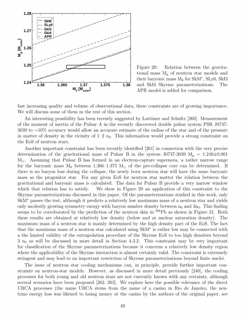
1.36 1.365 1.37 1.375 1.38M0 [Msolar]

1.24

1.25

1.26

1.27

1.28M

g [

Mso

lar]

SkM*

SLy6SkI3SkI4APR

Figure 20: Relation between the gravita-tional mass Mg of neutron star models andtheir baryonic mass M0 for SkM∗, SLy6, SkI3and SkI4 Skyrme parameterizations. TheAPR model is added for comparison.

fast increasing quality and volume of observational data, these constraints are of growing importance.We will discuss some of them in the rest of this section.

An interesting possibility has been recently suggested by Lattimer and Schultz [260]. Measurementof the moment of inertia of the Pulsar A in the recently discovered double pulsar system PSR J0737-3039 to ∼10% accuracy would allow an accurate estimate of the radius of the star and of the pressurein matter of density in the vicinity of 1–2 n0. This information would provide a strong constraint onthe EoS of neutron stars.

Another important constraint has been recently identified [261] in connection with the very precisedetermination of the gravitational mass of Pulsar B in the system J0737-3039 Mg = 1.249±0.001M⊙. Assuming that Pulsar B has formed in an electron-capture supernova, a rather narrow rangefor the baryonic mass M0 between 1.366–1.375 M⊙ of the pre-collapse core can be determined. Ifthere is no baryon loss during the collapse, the newly born neutron star will have the same baryonicmass as the progenitor star. For any given EoS for neutron star matter the relation between thegravitational and baryonic mass is calculated. The data for Pulsar B provide a very narrow windowwhich that relation has to satisfy. We show in Figure 20 an application of this constraint to theSkyrme parameterizations discussed in this paper. Of the parameterizations studied in this work, onlySkM∗ passes the test, although it predicts a relatively low maximum mass of a neutron star and yieldsonly modestly growing symmetry energy with baryon number density between n0 and 3n0. This findingseems to be corroborated by the prediction of the neutron skin in 208Pb as shown in Figure 21. Boththese results are obtained at relatively low density (below and at nuclear saturation density). Themaximum mass of a neutron star is mainly determined by the high density part of the EoS. The factthat the maximum mass of a neutron star calculated using SkM∗ is rather low may be connected witha the limited validity of the extrapolation procedure of the Skyrme EoS to too high densities beyond3 n0 as will be discussed in more detail in Section 4.3.2. This constraint may be very importantfor classification of the Skyrme parameterizations because it concerns a relatively low density regionwhere the applicability of the Skyrme interaction is almost certainly valid. The constraint is extremelystringent and may lead to an important restriction of Skyrme parameterizations beyond finite nuclei.

The issue of neutron star cooling mechanisms can, in principle, provide further important con-straints on neutron-star models. However, as discussed in more detail previously [240], the coolingprocesses for both young and old neutron stars are not currently known with any certainty, althoughseveral scenarios have been proposed [262, 263]. We explore here the possible relevance of the directURCA processes (the name URCA stems from the name of a casino in Rio de Janeiro; the neu-trino energy loss was likened to losing money at the casino by the authors of the original paper, see

49

Figure 21: Calculated neutron skin in 208Pbfor SkM∗, SLy6, SkI3 and SkI4 Skyrme pa-rameterizations is displayed as a function ofthe maximum mass of a neutron star, calcu-lated using EoS based on the same parame-terization. The straight line shows the resultof linear regression.

0.5 1 1.5 2 2.5Mg [Msolar]

0.1

0.15

0.2

0.25

r n -

rp [

fm]

SkM*

BSk1

SkP

SLy6

SkI4

SkI3

http://en.wikipedia.org/wiki/Urca process) given by

n −→ p + l + νl, p + l −→ n + νl, (48)

(where l stands for the leptons being considered here – electrons and muons) within the context ofthe Skyrme parameterizations studied in this paper. For this direct URCA process to take place, therelative components of the BEM must satisfy the appropriate conditions for conservation of energy andmomentum: y

1/3n < y

1/3p + y

1/3e and y

1/3n < y

1/3p + y

1/3µ . It has been argued that this will be satisfied

only at densities n several times larger than the nuclear saturation density n0 [264, 265, 266] when theproton fraction in BEM reaches a threshold value of ∼14%. It follows from (41) that the steeper theincrease of the symmetry energy with increasing number density, the faster will be the growth of theproton fraction yp. The results for the examples of the Skyrme parameterizations investigated here arerather interesting. SkM∗ does not satisfy the conditions for occurrence of the direct URCA process atany density. This is in contrast to SkI3 and SkI4 for which the threshold density (and correspondingmass) for the URCA process to take place is rather low (nURCA = 0.26 (MURCA = 0.90 M⊙) and 0.50fm−3 (MURCA = 1.59 M⊙), respectively) and SLy6 for which the direct URCA process can happenonly at nURCA = 1.18 (MURCA = 2.05 M⊙). The latter critical density and mass are equal to thosecalculated in maximum mass model with the SLy6 EoS. However, we note that there are alternativedirect URCA processes involving hyperons and thus this constraint, although interesting, is rather weak.Nevertheless an understanding of the cooling mechanism of neutron stars is important and the Skyrmeinteraction plays a significant role in these models [262]. We note that very recently a new constraintfor the direct URCA cooling mechanism has been suggested, based on analysis of population synthesisscenarios [267, 268]. It finds that direct URCA process (48) should not happen in neutron stars withmasses lower than ∼1.5 M⊙ (see Table 4)

It is intriguing to point out that the correlation between the properties of neutron matter and theneutron skin in finite nuclei, discussed generally in Section 3.1.3, can be extended to the correlationbetween maximum mass of a neutron star and the neutron skin in neutron heavy nuclei. Models of finitenuclei include surface and Coulomb effects, not present in calculation of the symmetry energy in nuclearmatter and yet the distinction between Skyrme parameterizations on the basis of the density dependence

of the symmetry energy is seen. As demonstrated in Figure 21, the Skyrme parameterizations with thesteepest increase of the symmetry energy with growing density that predict the highest maximum massof the cold neutron star, also predict the thickest neutron skin. We show this effect for Pb208 but it alsoexists in 132Sn, 122Zr, 78Ni and 48Ca, as reported in [269].

The Skyrme interaction has also been employed in a more subtle context of nuclear matter andneutron star theory. The onset of ferromagnetic instabilities in spin-polarized neutron matter at zero

50

and finite temperature has been investigated and identified for the SLy6 and SkI3 parameter sets [270].It has been shown that a new constraint on the Skyrme parameters can be derived to avoid theseinstabilities. The instability with respect to ferromagnetic collapse was also studied in terms of Landauparameters in symmetric and neutron matter and with respect to the constraint that the velocity ofsound has to remain smaller than the speed of light [271]. A set of 6 new Skyrme parameterizationshas been developed using parameters obeying the suggested constraints. It is interesting to note thatall these parameterizations predict decreasing symmetry energy at high densities [28].

4.3.2 Validity of the Skyrme model in high density matter: Hyperons and quark matterin neutron stars?

The current trend in the development of modern effective nuclear interactions is their applicabilityin finite nuclei as well as in infinite nuclear matter. In particular, the study of asymmetric nuclearmatter (with neutron-proton ratio 0 ≤ I ≤ 1) and pure neutron matter are of importance as anextrapolation point connecting finite nuclei at the line of stability, nuclei at the neutron drip line andsome density regions of neutron stars. One has to realize that all effective nuclear interactions in usetoday have parameters fitted to known properties of finite nuclei at or close to the stability line andsometime properties of nuclear matter at saturation density. The isospin and density dependence ofthese parameters is not known. Nevertheless we routinely extend the use of these parameters up to thedrip lines and expect them to work. The validity of this procedure is by no means guaranteed. Manyaspects of nuclear interactions (apart from surface effects) can be tested in infinite nuclear matter andit is desirable to make such calculations. The usual argument against this procedure is that modelslike SHF should not be used beyond nuclear saturation density. This is a matter of debate. Thegeneral consensus is that relativistic effects are small up to 2–3 n0 [225] and the Skyrme interactionis well justified for the description of nuclear matter consisting of nucleons and leptons (no strangebaryons or mesons)(see e.g. [225]). Indeed, in the degenerate fermi gas model, even at density ∼0.5fm−3, the relativistic correction to the mean energy of nucleons is about 10% which makes this densityacceptable from that point of view. Furthermore, the requirement of low momentum approximation inthe derivation of the Skyrme functional [54] sets a limit of about (πk−1

F > mπc = 1.4 fm) which infersthe same limiting density of 0.5 fm−3.

However, we reiterate that SHF describes only the nucleonic part of star matter. At high densityand temperature it is likely that heavy baryons and mesons will emerge at some point and contribute tothe total energy of dense matter. Simple estimates of the threshold for Λ and Σ±,0 hyperons just basedon their rest-mass, were discussed in [28] showing a possibility that these particles will exist in matterat 3 n0 and even below (1.5–2.0 n0). This simple estimate neglects the contribution to the thresholdenergy from the hyperon-nucleon and hyperon-hyperon interaction, which is unknown at present andhas been modeled in a variety of ways, mainly in relativistic models (see e.g. [234, 247, 250]), againpredicting hyperon creation close to, or below the 3 n0.

Another issue that is of even more wide ranging consequence is the question of the critical densitywhen nucleons will start to loose their identity and (partially) deconfined quark matter will emerge.At densities of about 3 n0 the nucleons will start to overlap and formation of six-quark bags andincreasing interaction strength between quarks of different nucleons will become more likely. Again,some calculations predict this critical density to be below n0 [234, 250]. Clearly no model based onnucleon degrees of freedom should be used for the description of matter with a significant deconfinedquark component.

Non-nucleonic components in nuclear matter will affect the EoS, in particular they will tend todecrease the slope of E as a function of density (the EoS softens). As it was shown above, this affectsall the observables of dense matter and other quantities like the maximum mass of cold neutron stars.Furthermore, it is important to realize that if we limit the EoS only to hadronic degrees of freedom,

51

current neutron star models are not strictly speaking valid at the baryon number densities of about 6–10n0, needed to calculate maximum mass models because at these densities nucleons and hyperons arelikely to loose their identity as composite particles and make a partial or possibly complete transitionto quark matter. Following this logic, the neutron star models shown in Figure 19 should be calculatedonly up to masses and radii indicated by circles on the Mg–R curves and the maximum mass of coldneutron stars would not be obtainable from such models.

4.3.3 Inhomogeneous matter.

In the previous sections, we discussed applications of SHF to models of homogeneous nuclear matterconsisting of unbound baryons and leptons. However, there is a large inhomogeneous phase of matterat lower densities that is present in crusts of neutron stars and forms a part of the collapsing core attype II supernovae. As already mentioned above, at densities below ∼ 6×10−11 fm−3 the matter in thisground state consists of 56Fe nuclei arranged in a lattice to minimize their Coulomb energy. A fractionof electrons are bound to the 56Fe nuclei. In the density range ∼ 6× 10−11 fm−3 < n < 2.5× 10−4 fm−3

the equilibrium nuclei, now immersed in a relativistic electron gas but still distributed in a lattice,become more neutron-rich as electron capture and inverse β-decay take place while direct β-decay isinhibited by the lack of unoccupied electron states. At about 2.5 × 10−4 fm−3 (the neutron drip-line)finite nuclei cannot support the neutron excess and start to emit neutrons to continuum neutron states.From this density up to about 0.1 fm−3, where the transition to homogeneous nuclear matter occurs,there are still bound nucleons, coexisting with a free neutron and electron gases. The modeling ofthis most interesting region is difficult as equilibrium emerges as result of a delicate balance betweennuclear surface energy (favoring large nuclei) and the Coulomb energy, the sum of the positive nuclearself-energy and negative lattice-energy, which favors small nuclei. The current understanding is thatthe nuclei form exotic phases (‘the pasta phase’) like rods, slabs, tubes, inside-out bubbles, spaghetti orlasagna, stabilized by the Coulomb interaction and characterized by various crystal lattice structures[272, 241, 273].

The models used for the description of inhomogeneous matter phase fall into two categories. Oneuses the semi-empirical mass formula or the compressible liquid drop model (LDM) for the descriptionof finite nuclei and a separate model to calculate the free neutron gas energy density (e.g. [274, 275, 276,277]). The second category includes self-consistent models that use the same interaction to describethe nuclear matter inside and outside the finite nuclei (e.g. [251, 278, 272, 273]). The advantage ofthe second class of models is obvious as they include in a consistent way the effect of the externalnucleons on nuclei which are not isolated but embedded in the sea of neutrons. The main interest ofthese calculations has focused on subnuclear densities, in particular the ‘pasta’ phase and the locationand properties of the phase transition between homogeneous and inhomogeneous matter. We note thatthere is no need for a self-consistent calculation of homogeneous matter as in this case the energy perparticle E and related quantities can be expressed analytically (24a).

A major group of models use SHF to determine the ground state energy of matter as a functionof density, temperature and proton fraction by minimization of the SHF energy density in coordinatespace. In this way the equilibrium energy per particle can be calculated as a continuous function ofdensity and the composition of nuclear matter is determined naturally without a priori assumptionsabout particular physical processes in certain density regions. One of the first models of this kind wasdeveloped by Bonche and Vautherin [279] for inhomogeneous matter assuming spherical symmetry (1Dspace) using the SkM and RPB Skyrme interactions. Later it was adopted by Hillebrandt and Wolff[280] with RATP, Ska and SkM Skyrme parameterizations for tabulation of the EoS in a dense grid ofenergy density, temperature (or entropy) and electron fraction for use in hydrodynamical codes (for moredetails see section 4.3.4). Pethick et al. [278] used the Skyrme1′, FPS and FPS21 parameterizationsin their EoS. The Gogny parameterization D1 has been also used to construct finite temperature EoS

52

[281, 282] based on the application of the variational principle to the thermodynamical potential withspecial attention to the liquid-gas phase transition. A semi-classical approximation to SHF, the ETFSImethod, with the parameterizations RATP, SkM∗ and SkSC4–10 was also applied to derive EoS atfinite temperatures for inhomogeneous [283] and homogeneous [284] nuclear matter under conditionsappropriate to a collapsing star assuming spherical symmetry. The EoS based on the RMF theory withthe TM1 parameter set for the RMF Lagrangian was used in modeling supernova physics by Shen etal., [285]. Both, homogeneous and inhomogeneous, matter are treated within the model. However, theinhomogeneous matter is not calculated fully self-consistently but is approximated as a b.c.c latticeof spherical nuclei and the free energy is minimized with respect to cell volume, proton and neutronradii and surface diffuseness of the nuclei and densities of the outside neutron and electron gases.Menezes and Providencia [250] used RMF to construct EOS of mixed stars formed by hadronic andquark matter in β equilibrium at finite temperature. The non-linear Walecka model and the MIT Bagand Nambu-Jona-Lasinio models were used for the hadronic and quark matter, respectively.

The major limitation of the models discussed so far, i.e. the assumption of spherical symmetryfor inhomogeneous matter, has been removed in the recent work of Magierski and Heenen [273] whotreated cold (T = 0) nuclear matter in the density region of the ‘pasta’ phase for the first time fullyself-consistently in 3D coordinate space (allowing for triaxial shapes) using SHF with SLy4 and SLy7parameterizations. The SHF equations were solved in a rectangular box with periodic boundary con-ditions. This includes naturally shell effects in neutron gas and pairing. In calculation of the Coulombenergy, the model goes beyond the Wigner-Seitz approximation of spherical cells (assumed in all thepreviously mentioned models) and includes both interactions between nuclei on different lattice sitesand between protons and electrons. Unfortunately no comparative study has been done as yet to sys-tematically explore the sensitivity of properties of inhomogeneous matter to the choice of the SHFparameterization in comparison with the other models.

4.3.4 Hot matter and type II (core-collapse) supernova models.

The most sought after constraint on EoS in hot matter would be based on success in modeling a typeII core-collapse supernova. There is no doubt that the supernova phenomenon exists in nature and isaccompanied by an explosion. Current models fail to reproduce this explosion. One of the possiblesolutions of this problem lies in the improvement of the EoS since the EoS at subnuclear densitiescontrols the rate of collapse, the amount of de-leptonization and thus the size of the collapsing core andthe bounce density. During the supernova collapse and the birth of a proto-neutron star the mattercan reach temperatures up to 20 MeV and thus the finite temperature EoS is used. The density atbounce of the collapsing core (for a detailed description of the core collapse mechanism see e.g. [286])goes up to 1.5–2.0 n0 and thus includes both homogeneous and inhomogeneous phases and the phasetransition between the two. Moreover, it may be just reaching the threshold for the appearance ofexotic components, like strange baryons and mesons, with possibly a phase transition to quark matterat the upper end of the density region. The timescale for supernova collapse is believed to be oforder of a second and the matter does have enough time to reach β equilibrium throughout the rapidchanges. Thus the calculation has to be performed for a fixed ratio of neutrons and protons, usuallyy taken yp ∼ 0.3 [286] and a relevant range of densities and temperatures. There are so far twoexamples of a finite temperature EoS, based on SHF, for use in supernova simulation codes. The earlycalculations of Hillebrandt and Wolff, mentioned in the previous section, used a spherically symmetricalSHF model (1D) [280]. As a new development, Newton and Stone [224, 287] extended the previous SHF3D calculation [273] to finite temperature and wide range of densities for use in supernova simulationmodels. The calculation scheme (using SkM∗ at present) treats the finite nuclei and the neutron gasin the ’pasta’ phase as one entity and naturally allows effects such as (i) neutron drip, which resultsin an external neutron gas, (ii) the variety of exotic nuclear shapes expected for extremely neutron

53

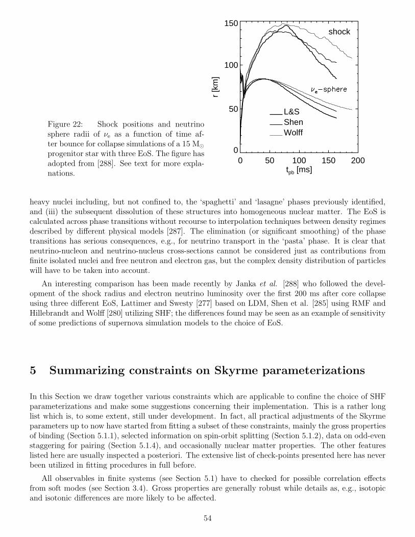
Figure 22: Shock positions and neutrinosphere radii of νe as a function of time af-ter bounce for collapse simulations of a 15 M⊙

progenitor star with three EoS. The figure hasadopted from [288]. See text for more expla-nations.

0 50 100 150 200tpb [ms]

0

50

100

150

r [k

m]

WolffShenL&S

shock

heavy nuclei including, but not confined to, the ‘spaghetti’ and ‘lasagne’ phases previously identified,and (iii) the subsequent dissolution of these structures into homogeneous nuclear matter. The EoS iscalculated across phase transitions without recourse to interpolation techniques between density regimesdescribed by different physical models [287]. The elimination (or significant smoothing) of the phasetransitions has serious consequences, e.g., for neutrino transport in the ‘pasta’ phase. It is clear thatneutrino-nucleon and neutrino-nucleus cross-sections cannot be considered just as contributions fromfinite isolated nuclei and free neutron and electron gas, but the complex density distribution of particleswill have to be taken into account.

An interesting comparison has been made recently by Janka et al. [288] who followed the devel-opment of the shock radius and electron neutrino luminosity over the first 200 ms after core collapseusing three different EoS, Lattimer and Swesty [277] based on LDM, Shen et al. [285] using RMF andHillebrandt and Wolff [280] utilizing SHF; the differences found may be seen as an example of sensitivityof some predictions of supernova simulation models to the choice of EoS.

5 Summarizing constraints on Skyrme parameterizations

In this Section we draw together various constraints which are applicable to confine the choice of SHFparameterizations and make some suggestions concerning their implementation. This is a rather longlist which is, to some extent, still under development. In fact, all practical adjustments of the Skyrmeparameters up to now have started from fitting a subset of these constraints, mainly the gross propertiesof binding (Section 5.1.1), selected information on spin-orbit splitting (Section 5.1.2), data on odd-evenstaggering for pairing (Section 5.1.4), and occasionally nuclear matter properties. The other featureslisted here are usually inspected a posteriori. The extensive list of check-points presented here has neverbeen utilized in fitting procedures in full before.

All observables in finite systems (see Section 5.1) have to checked for possible correlation effectsfrom soft modes (see Section 3.4). Gross properties are generally robust while details as, e.g., isotopicand isotonic differences are more likely to be affected.

54

5.1 Finite nuclei

5.1.1 Gross properties: energy, charge radii

The most important features to be properly reproduced are the nuclear bulk properties:

binding energy EB,charge r.m.s. radius rch,charge diffraction radius Rch, andcharge surface thickness σch.

These are usually considered in a large selection of spherical (doubly magic and semi-magic) nuclei.Thus nuclei which are likely to carry sizeable correlations should be excluded. This holds, e.g., fornuclei with N = Z because of a rather large Wigner energy. Light nuclei should also be scrutinized forcorrelation effects. The best possible selection of experimental data is still a question of debate.

5.1.2 Spin-orbit splitting

The spin-orbit splitting is automatically provided in RMF but has to be adjusted ‘by hand’ in SHF.Experimental data for this adjustment are taken from the spectra of doubly-magic nuclei, for levelswhich are close to the Fermi energy and thus rather free from polarization and correlation effects. Upto now, almost all fits have considered spin-orbit splittings only in 16O and 208Pb. Other options forwhich good data exist, such as 40Ca, 48Ca, 90Zr, or 132Sn, should be exploited.

5.1.3 Neutron radii

Information on neutron radii rn and/or neutron skin rn − rp are most useful to pin down the isovectorproperties of the parameterization, particularly the symmetry energy asym. The problem here is that rn

is deduced from model-dependent analysis of scattering experiments. To overcome this obstacle, directmodeling of the scattering process by SHF should be considered.

5.1.4 Energy differences

The odd-even staggering of binding energies in medium heavy and heavy nuclei is used to adjust thepairing strength. It is recommended to use the staggering from the five-point difference formula tominimize perturbation from competing polarization (Jahn-Teller effect) [73].

Two-proton and two-neutron separation energies can supply information on shell structure, partic-ularly on the magnitude of shell gaps. A proper description is crucial for the predictive value of SHFin application to the r-process (see Section 3.3). However, one has to be aware of possible correlationeffects on this quantity (see Section 3.4.2).

5.1.5 Isotopic shifts

The isotope shift in radii of Pb can be used a test of the strength of the isovector spin-orbit force [56].

Much information is contained in other chains to, such as the negligible difference in charge radiibetween 40Ca and 48Ca, or the large shift in certain regions of, e.g., Sr or Hg isotopes. However, thesechains are likely to include sizeable correlation effects.

55

5.1.6 Deformations

More advanced test cases can be found in properties of deformed nuclei, their ground state deformationsand rotational bands. A possible selection may be:

deformation in heaviest nuclei (264Hs),triaxial deformation (138Sm, 188Os),octupole deformation (222,224Th, 146Ba),super-deformed states (192,194Hg, 194Pb,238U),hyper-deformed states (232Sm) ,prolate-oblate competition (184,186Pt, 184,186Hg),spherical-to-deformed transition in heavy Zr isotopes 96,98,100Zr, and/or fission barriers in actinides.

Deformation properties are often sensitive to details of the shell structure and constitute extremelycritical tests. Nuclei with well developed stable deformation are generally well described within a mean-field model. Transitional regime, although very interesting, has to be investigated for possible influenceof correlation effects.

5.1.7 Excitation properties

Excitation properties provide a rich pool of information. Giant resonances in heavy nuclei are closelyrelated to key properties of nuclear matter such as incompressibility (isoscalar monopole), symmetryenergy (isovector dipole), or effective mass (isoscalar quadrupole). The isovector dipole resonance inlight nuclei is not yet under control and presents a big puzzle (see Section 3.2.1).

Excitation with unnatural parity as, e g., the Gamow-Teller resonances can serve to fix the not sowell known properties of SHF in the spin channel (see Section 3.2.2). There is still a long road aheadin exploiting these aspects.

Low-energy quadrupole excitations carry combined information on shell structure (near doubly magicnuclei) and on pairing. However, the modeling has yet to be improved in order to truly optimize thelarge amplitude collective path (see Section 3.4.1).

5.2 Nuclear matter and neutron star models

The constraints one nuclear matter properties are of two types. The first concerns expected values ofsome empirical quantities at nuclear saturation density n0. These values and/or their lower and upperlimits, coming from merging data obtained from LDM or indirectly from experiments as discussed inSection 4.2.1, are summarized in Table 3. The LDM values are an extrapolation from finite nuclei data,similarly as the various SHF values. They serve merely as an orientation to the extend that modelswhich deviate too much from these ‘commonly accepted values’ are to be questioned.

The second type of constraint is given by the density dependence of energy per particle E0, theasymmetry coefficient asym(n0), the isoscalar effective nucleon mass m∗

s/m and derived quantities likethe pressure, incompressibility and the velocity of sound in SNM, PNM and BEM. There is no firmlybased set of values of these quantities and their various dependences. The best that can be done isto compare their predicted values to a ‘realistic’ ab initio theoretical model. However, they have aprofound effect on the EoS used in neutron star models which can indeed in turn can be tested againstobservational data. Although the data are still lacking desired accuracy and are related to each other(usually as a function of the star mass), they have already proven to be powerful enough to eliminatesome EoS (and thus Skyrme parameterizations) from use in neutron star models [28] although theyperform well in finite nuclei. Considerable progress in increasing the quality of data on cold neutronstars is expected in the near future when, for example, there is hope to have independent values of

56

Table 3: Summary of constraints from nuclear matter at saturation density. The “commonly acceptedvalues” are taken from the LDM as published in [26, 236]. The calculated values for the Skyrmeparameterizations used in the review are given for illustration. All symbols are explained in the text.

Constraint LDM SkM∗ SkP SLy6 SkI3 SkI4 BSk1n0 [fm−3] 0.16 ± 0.01 0.160 0.163 0.159 0.158 0.160 0.157E0 [MeV] -16.1 ± 0.1 -15.77 -15.95 -15.92 -15.98 -15.94 -15.80K∞ [MeV] 230 ± 20 217.5 201.9 230.8 259.0 249.1 232.1asym(n0) [MeV] 31 ± 1.5 30.06 30.02 32.00 34.89 29.54 27.82m∗

s/m 1.0 0.79 1.00 0.69 0.58 0.65 1.05

Table 4: Summary of constraints from properties of cold neutron stars. Fullfilment of some of theseconstraints for the sample Skyrme parameterizations is indicated by ‘+’ (fulfilled), ‘(+)’ (fulfilled butthe constraint is weak), ‘-’ (failed). ‘0’ stays for undecided as either the constraints is uncertain atpresent or the property was not tested for the parameterization in question. Symbols are explained inthe text.

Constraint Expected value SkM∗ SkP SLy6 SkI3 SkI4 BSk1Mmax [M⊙] 2.1± 0.2 0 - + + + -Rmax [km] 8–15 + - + + + -R1.4⊙ [km] 9–16 + - + + + -Ebin [1053 ergs] 3.8 ± 1.2 0 - 0 0 0 -ρcentr

max [1015 gcm−3] 0.5–4.0 (+) - (+) (+) (+) -M0 [M⊙] 1.356 < 1.375 + - - - - -MURCA [M⊙] > 1.5 0 - + 0 + -

neutron star radii rather than values determined as a function of the gravitational mass. The recentlyproposed method of its independent determination could be realized in a few years [260]. We list intable 4 the main constraints based on neutron star models.

Certain other constraints, such as those connected with polarized nuclear matter and its ferromag-netic collapse, have not been quantified as yet for the majority for SHF models and are yet to beexplored. We mention that very recently [268] a similar set of constraints has been suggested for testingeffective interactions used in EoS based on RMF models.

5.3 Supernova simulations

The most powerful constraint on the SHF equation of state would be achieving the explosion of thecore-collapse supernova model. It is important to reiterate that the density region at which this collapseis expected to happen (1.5–2.0 n0) is well within the expected window of validity of the SHF modelbeyond the saturation density. However these tests are rather complicated as there are certain otherfactors in the supernova process that may affect the occurrence of the explosion and their relation withthe EoS are not fully established. However, supernova physics offers a new ground for testing the SHFmodels which is just starting to be explored [190].

57

6 Conclusions

The application of the Skyrme Hartree-Fock model (SHF) to finite nuclei, nuclear matter and in as-trophysical contexts has been critically surveyed, with occasional consideration links of its relativisticcousin, the relativistic mean-field model, and to ab-initio models. SHF provides an effective energy-functional which is motivated by many-body theory and leaves about 6–12 free parameters which areadjusted phenomenologically. The functional is universal in the sense that it, in principle, applicableto all nuclei (except the very light) irrespective to their shape or shell structure. The current modelsusually calculate static and dynamical properties of even-even nuclei exactly and approximate modelsfor odd-A and odd-odd nuclei in some fashion, although an exact approach is in principle possible andis waiting to be implemented in SHF codes. Static observables include nuclear ground state bindingenergies, profile and shape of charge and neutron density distributions, nuclear radii and fission barriers.The SHF models provide, in the small-amplitude limit of TDHF, useful information on the excitationspectrum, particularly on the various giant resonances which form important features of the nuclearexcitation spectrum. Moreover, the large amplitude limit of TDHF covers a wide range of phenomena,low-lying collective modes, fission, rotational bands, fusion and nuclear collisions.

The overall global agreement of the SHF model with existing data is overwhelmingly good. Localdiscrepancies in SHF predictions, however, exist which is fully understandable because the effectivefunctionals has a simple analytical form and is preferably appropriate for reproducing smooth trends.Moreover, the isospin and density dependence of these parameters is not yet well known. It is oftenobserved that local deviation between SHF calculation and experiment is not statistical but exhibitssystematic trends which indicate aspects for future improvement (see Section 3.1.1). As an example,discrepancies between experimental and calculated two-neutron-separation energies may originate indetailed, but locally important, physics like shell effects, shape fluctuations and level densities at theFermi surface to which global observables have limited sensitivity. Similarly, the whole range of dy-namical nuclear properties is reproduced well by the SHF model, again with exception which constitutemajor challenges yet to be addressed (see Section 3.2). For example, no SHF parameterization cansimultaneously reproduce the average peak position of the GDR in heavy and light nuclei.

Discrepancies between results of SHF calculation and experimental data often originate from cor-relations beyond mean field (see Section 3.4). There is a large potential for systematic investigationof these effects that may lead to better understanding of the limitations of the SHF and similar self-consistent mean-field models. Another major improvement can be achieved by gradual elimination ofimperfections in fitting of the Skyrme energy functional. It is well known that due to mutual correlationbetween the variable parameters of the Skyrme functional, there is, in principle, an infinite number ofcombinations of the parameters which could be fitted to experimental data and produce results with anequally satisfactory agreement with experiment. There exists already a great manifold of such sets inthe literature and it is very difficult to make a well founded choice between them, in particular in cal-culations of properties of finite nuclei. This situation is not unique to SHF but a generic problem of alltypes of nuclear effective energy functionals. It is caused by the fact that an ab-initio derivation of thefunctionals is hindered by the uncertainty in the true nature and form of the genuine nucleon-nucleoninteraction in the nuclear environment.

One way forward in confining the manifold of permissible parameterizations is to systematicallyincrease the amount and variety of experimental data used in the fitting process. Attempts to use onlyone selected type of observable in fitting, like nuclear masses, and to ignore all the other experimentaldata, did not meet with real success. The common practice adopted in fitting of most parameterizationsis to use ground state properties of magic or semi-magic nuclei in the hope that these nuclei will be leastaffected by correlations beyond the mean field and that many effects like shape fluctuation, shell effectsand pairing may be neglected. The increasing amount of experimental information on nuclei far fromstability allows to include more stringent information, particularly concerning isovector properties of the

58

effective interactions. This should improve steadily the extrapolative power of SHF which is at presentstill rather unsatisfactory (i.e. the deviation between predictions of different SHF parameterizations isincreasing with growing distance from the stability line which causes extrapolation of SHF models to thedrip-line regions lacking credibility). Establishing more reliable extrapolations is the major challengefor future development because that is desperately needed for a variety of astrophysical applications,like understanding the r-process. The same holds for the construction of SHF based EoS for descriptionof nuclear matter under extreme conditions of high density and temperature that exists in neutron starand supernovae. Similarly, in terrestrial ‘extreme’ conditions, reliable EoS are desirable for modeling ofheavy-ion collision processes and investigations of super-heavy nuclei.

We believe it would be very beneficial to develop modern Skyrme parameter sets that would satisfysimultaneously the extended set of constraints summarized in Section 5. Although this will not createa unique set of the Skyrme parameters, it will give the best chance to create a model that would beapplicable on a global scale. It has been shown in Section 4 that properties of nuclear matter even atdensities below 3 n0 offer a sensitive test of the Skyrme parameterizations. It is plausible that extensionof the SHF models to systems with high values of isospin, like cold neutron stars, would provide adistant extrapolation point with the closed-shell stable nuclei at the other extreme and the neutron-drip-line nuclei between the two. This development may even give us a better insight into the physicalconnection between Skyrme parameters (or their selected combinations) and some nuclear propertiesand thus give more control over the model. As long as a quantitative performance of more fundamentalmodels of nuclear interactions, perhaps based on subnucleon degrees of freedom, is still ahead in thefuture, up-to-date SHF models are likely to remain an important tool in low-energy nuclear physics andastrophysics for some time to come.

7 Aknowledgements

We wish to thank N. J. Stone for reading of the manuscript and many constructive suggestions. Helpfulcomments of D. M. Brink, D. Dean, P. Guichon, W. R. Hix, P. Klupfel, K.-L. Kratz, J. C. Miller andB. Pfeiffer are gratefully acknowledged. This work has been supported by US DOE grant DE-FG02-94ER40834, from DOE Scientific Discovery through Advanced Computing Grant, and from the BMBF(project 06 ER 124).

59

A Appendix 1

A.1 Parameters of the sample group of Skyrme parametrisations in nu-

clear matter calculations

Parameters of the Skyrme parametrizations SkM∗, SkP, SLy6, SkI3, SkI4 and BSk1 are listed in Table 5.

Table 5: Parameters of the sample Skyrme interactions. For definitions see (11,12).

Skyrme B0 B′0 B1 B′

1 B3 B′3 α

SkM∗ -1983.75 -780.28 2924.06 974.69 34.688 34.063 0.166667SkP -2198.78 -1161.17 3507.93 1592.67 -0.000 44.642 0.166667SLy6 -1859.63 -1642.67 2563.69 3170.43 58.621 -26.016 0.166667SkI3 -1322.16 -712.47 1519.91 1816.40 96.258 -63.957 0.25SkI4 -1391.87 -839.84 1819.43 1995.55 69.927 -37.655 0.25BSk1 -1372.84 -1006.74 2520.88 2223.54 -6.277 0.000 0.333333

Skyrme t0 t1 t2 t3 x0 x1 x2 x3 αSkM∗ -2645.00 410.00 -135.00 15595.00 0.090 0.000 0.000 0.000 0.166667SkP -2931.70 320.62 -337.41 18708.96 0.292 0.653 -0.537 0.181 0.166667SLy6 -2479.50 462.18 -448.61 13673.00 0.825 -0.465 -1.000 1.355 0.166667SkI3 -1762.88 561.61 -227.09 8106.20 0.308 -1.172 -1.091 1.293 0.25SkI4 -1855.83 473.83 1006.86 9703.61 0.405 -2.889 -1.325 1.145 0.25BSk1 -1830.45 262.97 -296.45 13444.70 0.600 -0.500 -0.500 0.823 0.333333

References

[1] R. Machleidt and I. Slaus, J. Phys. G 27 (2001), R69.

[2] W. H. Dickhoff and H. Muther, Rep. Prog. Phys. 55 (1992), 1947.

[3] H. Heiselberg and Vijay Pandharipande, Annual Review of Nuclear and Particle Science 50 (2000),481.

[4] M. Lutz, B. Friman, and Ch. Appel, Phys. Lett. B474 (2000), 7.

[5] N. Kaiser, S. Fritsch, and W. Weise, Nucl. Phys. A700 (2002), 343.

[6] W. Weise, Nucl. Phys. A751 (2005), 565.

[7] H. Bohr, C. Providencia, and J. da Providencia, Phys. Rev. C71 (2005), 055203.

[8] P. Navratil, J. P. Vary, and B. R. Barrett, Phys. Rev. C 62 (2000), 054311.

[9] C. Forseen, P. Navratil, W. E. Ormand, and E. Caurier, Phys. Rev. C71 (2005), 044312.

[10] S. C. Pieper and R. B. Wiringa, Phys. Rev. C70 (2004), 054325.

[11] M. Wloch, D.J. Dean, J.R. Gour, M. Hjorth-Jensen, K. Kowalski, T. Papenbrok, and P. Piecuch,Phys. Rev. Lett. 94 (2005), 212501.

60

[12] R. Roth, H. Hergert, P Papakonstantinou, T. Neff, and H. Feldmeier, PRC 72 (2005), 034002.

[13] P. Navratil, private communication, 2006.

[14] P. Moller, J. R. Nix, and K.-L. Kratz, At. Data Nucl. Data Tables 66 (1997), 131.

[15] W. D. Myers and W. J. Swiatecki, Annual Review of Nuclear and Particle Science 32 (1982), 309.

[16] S. G. Nilsson and I. Ragnarsson, Shapes and shells in nuclear structure, Cambridge UniversityPress, Cambridge, 1995.

[17] P. Moller, J.R. Nix, W.D. Myers, and W.J. Swiatecki, At. Data Nucl. Data Tab. 59 (1995), 185.

[18] S. E. Koonin, D. J. Dean, and K. Langanke, Phys. Rep. 278 (1997), 1.

[19] I. Zh. Petkov and M. V. Stoitsov, Nuclear density functional theory, Clarendon Press, Oxford,1991.

[20] P.-G. Reinhard, Inst. Phys. Conf. Ser. 132 (1992), 157.

[21] R. M. Dreizler and E. K. U. Gross, Density functional theory, Springer, Berlin, Heidelberg, NewYork, 1990.

[22] M. Bender, P.-H. Heenen, and P.-G. Reinhard, Rev. Mod. Phys. 75 (2003), 121.

[23] M. Brack and P. Quentin, Nucl. Phys. A361 (1981), 35.

[24] M. Brack, C. Guet, and H.-B. Haakansson, Phys. Rep. 123 (1985), 275.

[25] Y. Aboussir, J. M. Pearson, A. K. Dutta, and F. Tondeur, Nucl. Phys. A549 (1992), 155.

[26] W. D. Myers and W. Swiatecki, Phys. Rev. C 58 (1998), 3368.

[27] , Phys. Rev. C 60 (2000), 054313.

[28] J. Rikovska Stone, J. C. Miller, R. Koncewicz, P. D. Stevenson, and M. R. Strayer, Phys. Rev.C68 (2003), 034324.

[29] G. Dissertori, I.G. Knowels, and M. Schmelling, Quantum chromodynamics: High energy experi-

ments and theory, Clarendon Press, Oxford, 2003.

[30] P.-G. Reinhard and C. Toepffer, Int. J. Mod. Phys. E3 (1994), 435.

[31] V. R. Pandharipande, I. Sick, and P. K. A. deWitt Huberts, Rev. Mod. Phys. 69 (1997), 981.

[32] H. Kummel, K. Luhrmann, and J. Zabolitzky, Phys. Rep. 36 (1978), 1.

[33] R. D. Mattuck and A. Theumann, Adv. Phys. 20 (1971), 721.

[34] R. Brockmann and R. Machleidt, Phys. Rev. C 42 (1990), 1965.

[35] P.-G. Reinhard and D. Drechsel, Z. Phys. A290 (1979), 85.

[36] W.M. Alberico, A. Molinari, R. Cenni, and M.B. Johnson, Ann. Phys.(NY) 138 (1982), 178.

[37] A.D. Jackson, A. Lande, and R.A. Smith, Phys. Rep. 86 (1982), 55.

61

[38] P. Ring and P. Schuck, The nuclear many-body problem, Springer–Verl., New York, Heidelberg,Berlin, 1980.

[39] P.-G. Reinhard and K. Goeke, Rep. Prog. Phys. 50 (1987), 1.

[40] Giu Do Dang, A. Klein, and N. R. Walet, Phys. Rep. 335 (2000), 93.

[41] H. Reinhardt, Nucl. Phys. A 369 (1981), 122.

[42] K. Goeke, P.-G. Reinhard, and H. Reinhardt, Nucl. Phys. A378 (1982), 474.

[43] , Phys. Lett. 118B (1982), 1.

[44] A. Klein and E.R. Marshalek, Rev. Mod. Phys. 63 (1991), 375.

[45] C. Toepffer and P.-G. Reinhard, Ann. Phys. 181 (1988), 1.

[46] C. Fuchs, Prog. Part. Nuc. Phys. 56 (2006), 1.

[47] T.T.S. Kuo and E. Osnes, Nucl Phys. A 205 (1973), 1.

[48] J. W. Negele and D. Vautherin, Phys. Rev. C5 (1972), 1472.

[49] S. Weisgerber and P.-G. Reinhard, Z. Phys. D 23 (1992), 275.

[50] P.-G. Reinhard and E. W. Otten, Nucl. Phys. A420 (1984), 173.

[51] T. H. R. Skyrme, Phil. Mag. 1 (1956), 1043.

[52] , Nucl. Phys. 9 (1959), 615.

[53] D. Vautherin and D. M. Brink, Phys. Lett. 32B (1970), 149.

[54] , Phys. Rev. C5 (1972), 626.

[55] S. Krewald, V. Klemt, J. Speth, and A. Faessler, Nucl Phys. A 281 (1977), 166.

[56] P.-G. Reinhard and H. Flocard, Nucl. Phys. A584 (1995), 467.

[57] Y. M. Engel, D. M. Brink, K. Goeke, S. J. Krieger, and D. Vautherin, Nucl. Phys. A249 (1975),215.

[58] J. C. Slater, Phys. Rev. 81 (1951), 385.

[59] K. Rutz, M. Bender, P.-G. Reinhard, and J. A. Maruhn, Phys. Lett. B468 (1999), 1.

[60] A. Sulaksono, T. Burvenich, J. A. Maruhn, P.-G. Reinhard, and W. Greiner, Ann. Phys. (N.Y.)308 (2003), 354.

[61] K. W. Schmid and P.-G. Reinhard, Nucl. Phys. A530 (1991), 283.

[62] M. N. Butler, D. W. L. Sprung, and J. Martorell, Nucl. Phys. A422 (1984), 157.

[63] F. Barranco, R. A. Broglia, G. Gori, E. Vigezzi, P. F. Bortignon, and J. Terasaki, Phys. Rev.Lett. 83 (1999), 2147.

[64] J. Terasaki, H. Flocard, P.-H. Heenen, and P. Bonche, Phys. Rev. C 55 (1997), 1231.

62

[65] J. Dobaczewski, W. Nazarewicz, and P.-G. Reinhard, Nucl. Phys. A693 (2001), 361.

[66] J. Decharge and D. Gogny, Phys. Rev. C21 (1980), 1568.

[67] P. Ring, Prog. Part. Nucl. Phys. 37 (1996), 193.

[68] J. B locki and H. Flocard, Nucl. Phys. A273 (1976), 45.

[69] T. Gonzalez-Llarena, J. L. Egido, G. A. Lalazissis, and P. Ring, Phys. Lett. B379 (1996), 13.

[70] J. Dobaczewski, H. Flocard, and J. Treiner, Nucl. Phys. A422 (1984), 103.

[71] P. Bonche, H. Flocard, P.-H. Heenen, S. J. Krieger, and M. S. Weiss, Nucl. Phys. A443 (1985),39.

[72] S. J. Krieger, P. Bonche, H. Flocard, P. Quentin, and M. S. Weiss, Nucl. Phys. A517 (1990), 275.

[73] M. Bender, K. Rutz, P.-G. Reinhard, and J. A. Maruhn, Eur. Phys. J. A8 (2000), 59.

[74] M. Anguiano, J. L. Egido, and L. M. Robledo, Nucl. Phys. A696 (2001), 467.

[75] J. Dobaczewski and J. Dudek, Comput. Phys. Commun. 131 (2000), 164.

[76] V. Blum, G. Lauritsch, J. A. Maruhn, and P.-G. Reinhard, J. Comput. Phys. 100 (1992), 364.

[77] P.-G. Reinhard, Computational Nuclear Physics 1 – Nuclear Structure (K. Langanke, J. A.Maruhn, and S. E. Koonin, eds.), Springer, Berlin, Heidelberg, New York, 1991, p. 28.

[78] K. Rutz, M. Bender, P.-G. Reinhard, J. A. Maruhn, and W. Greiner, Nucl. Phys. A634 (1998),67.

[79] J. Friedrich and N. Vogler, Nucl. Phys. A373 (1982), 192.

[80] J. L. Friar and J. W. Negele, Adv. Nucl. Phys. 8 (1975), 219.

[81] G. G. Simon, C. Schmitt, F. Borkowski, and V. H. Walther, Nucl. Phys. A333 (1980), 381.

[82] V. H. Walther, private communication, 1986.

[83] P.-G. Reinhard, Phys. Lett. A169 (1992), 281.

[84] S. Mizutori, J. Dobaczewski, G. A. Lalazissis, W. Nazarewicz, and P.-G. Reinhard, Phys. Rev. C61 (2000), 044326.

[85] M. Samyn, S. Goriely, P.-H. Heenen, J. M. Pearson, and F. Tondeur, Nucl. Phys. A700 (2002),142.

[86] W. Satu la, J. Dobaczewski, and W. Nazarewicz, Phys. Rev. Lett. 81 (1998), 3599.

[87] E. Chabanat, P. Bonche, P. Haensel, J. Meyer, and R. Schaeffer, Nucl. Phys. A635 (1998), 231,Nucl. Phys. A643, 441(E).

[88] J. Friedrich and P.-G. Reinhard, Phys. Rev. C 33 (1986), 335.

[89] W. Satu la, D. J. Dean, J. Gary, S. Mizutori, and W. Nazarewicz, Phys. Lett. B407 (1997), 103.

[90] J. Bartel, P. Quentin, M. Brack, C. Guet, and H.-B. Hakansson, Nucl. Phys. A386 (1982), 79.

63

[91] T. Burvenich, D. Madland, J. A. Maruhn, and P.-G. Reinhard, Phys. Rev. C 65 (2002), 044308.

[92] M. Rufa, P.-G. Reinhard, J. A. Maruhn, W. Greiner, and M. R. Strayer, Phys. Rev. C 38 (1988),390.

[93] G. A. Lalazissis, J. Konig, and P. Ring, Phys. Rev. C 55 (1997), 540.

[94] P.-G. Reinhard, Rep. Prog. Phys. 52 (1989), 439.

[95] Y. K. Gambhir, P. Ring, and A. Thimet, Ann. Phys. (NY) 198 (1990), 132.

[96] P.-G. Reinhard, M. Bender, W. Nazarewicz, and T. Vertse, 73 (2006), 014309.

[97] J. Boguta and A. R. Bodmer, Nucl. Phys. A292 (1977), 413.

[98] B. D. Serot and J. D. Walecka, Phys. Lett. 87B (1979), 172.

[99] , Adv. Nucl. Phys. 16 (1986), 1.

[100] D. Vretenar, A.V. Afanasjev, G.A. Lalazissis, and P. Ring, Phys. Rep. 409 (2005), 101.

[101] T. Hoch and P. Manakos, Z. Phys. A337 (1990), 383.

[102] S. Typel and H. H. Wolter, Nucl. Phys. A656 (1999), 331.

[103] F. Hofmann, C. M. Keil, and H. Lenske, Phys. Rev. C 64 (2001), 034314.

[104] T. Niksic, D. Vretenar, G.A. Lalazissis, and P. Ring, Phys. Rev. C 69 (2004), 047301.

[105] M. Thies, Nucl. Phys. A460 (1986), 636.

[106] D. Gogny, P. Pires, R. De, and Tourreil, Phys. Lett. 32B (1970), 591.

[107] M. Baldo, C. Maieron, P. Schuck, and X. Vinas, Nucl. Phys. A 736 (2004), 241.

[108] J. P. Perdew, K. Burke, and M. Ernzerhof, Phys. Rev. Lett. 77 (1996), 3865.

[109] L. G. Cao, U. Lombardo, C. W. Shen, and N. Van Giai, 73 (2006), 014313.

[110] M. Serra, T. Otsuka, Y. Akaishi, P. Ring, and S. Hirose, Prog. Theor. Phys. 113 (2005), 1009.

[111] J. Rong, Z.-Y. Ma, and N.V. Giai, Phys. Rev. C 73 (2006), 014614.

[112] C. Maieron, M. Baldo, G. F. Burgio, and H. J. Schultze, Phys. Rev. D70 (2004), 043010.

[113] R. M. Aguirre and A. L. De Paoli, Phys. Rev. C68 (2003), 055804.

[114] J. O. Andersen and M. Strickland, Phys. Rev. D66 (2002), 105001.

[115] P. A. M. Guichon and A. W. Thomas, Phys. Rev. Lett. 93 (2004), 132502.

[116] P. A. M. Guichon, K. Saito, E. N. Rodionov, and A. W. Thomas, Nucl. Phys. A601 (1996), 349.

[117] P. A. M. Guichon, H. H. Matevosyan, N. Sandulescu, and A. W. Thomas, arXiv:nucl-th/0603044(2006).

[118] M. Bender, K. Rutz, P.-G. Reinhard, J. A. Maruhn, and W. Greiner, Phys. Rev. C 60 (1999),034304.

64

[119] P. Pfeiffer, K. L. Kratz, F. K. Thielemann, and W. B. Walters, Nucl. Phys. A688 (2001), 308.

[120] B. Chen, J. Dobaczewski, K.-L. Kratz, K. Langanke, P. Pfeiffer, F.-K. Thielemann, and P. Vogel,Phys. Lett. 355B (1995), 37.

[121] M. Anselment, W. Faubel, S. Goring, A. Hanser, G. Meisel, H. Rebel, and G. Schatz, NPA 451(1986), 471.

[122] N. Tajima, P. Bonche, H. Flocard, P.-H. Heenen, and M. S. Weiss, Nucl. Phys. A551 (1993), 434.

[123] M. M. Sharma, G. A. Lalazissis, and P. Ring, Phys. Lett. B317 (1993), 9.

[124] M. M. Sharma, G. A. Lalazissis, J. Konig, and P. Ring, Phys. Rev. Lett. 74 (1995), 3744.

[125] B. C. Clark and L. J. Kerr, Phys. Rev. E 68 (2003), 031204.

[126] C. J. Batty, E. Friedman, H. J. Gils, and H. Rebel, Adv. Nucl. Phys. 19 (1989), 1.

[127] B. A. Brown, Phys. Rev. Lett. 85 (2000), 5296.

[128] S. Typel and B. A. Brown, Phys. Rev. C 64 (2001), 027302.

[129] P.-G. Reinhard, Nucl. Phys. A649 (1999), 305c.

[130] D. Vretenar, N. Paar, T. Niksic, and P. Ring, Phys. Rev. Lett. 91 (2003), 2625021.

[131] A. T. Kruppa, M. Bender, W. Nazarewicz, P.-G. Reinhard, T. Vertse, and S. Cwiok, Phys. Rev.C 61 (2000), 034313.

[132] M. Bender, W. Nazarewicz, and P.-G. Reinhard, Phys. Lett. 515 (2001), 42.

[133] H. J. Specht, Rev. Mod. Phys. 46 (1974), 773.

[134] H. Flocard, P. Quentin, D. Vautherin, M. Veneroni, and A. K. Kerman, Nucl. Phys. A231 (1974),176.

[135] J.-F. Berger, M. Girod, and D. Gogny, Nucl. Phys. A428 (1984), 23c.

[136] V. Blum, J. A. Maruhn, P.-G. Reinhard, and W. Greiner, Phys. Lett. 323B (1994), 262.

[137] K. Rutz, J. A. Maruhn, P.-G. Reinhard, and W. Greiner, Nucl. Phys. A590 (1995), 680.

[138] M. Bender, K. Rutz, P.-G. Reinhard, and J. A. Maruhn, Eur. Phys. J. A7 (2000), 467.

[139] P.-G. Reinhard, Nucl. Phys. A261 (1976), 291.

[140] A. Mamdouh, J. M. Pearson, M. Rayet, and F. Tondeur, Nucl. Phys. A644 (1998), 389.

[141] T. Burvenich, M. Bender, J.A. Maruhn, and P.-G. Reinhard, Phys. Rev. C 69 (2004), 014307.

[142] M. Bender, private communication, 2004.

[143] Yu. Ts. Oganessian et al., Phys. Rev. Lett. 83 (1999), 3154.

[144] , Nature 400 (1999), 209.

[145] , Phys. Rev. C 63 (2001), 011301(R).

65

[146] J. W. Negele, Rev. Mod. Phys. 54 (1982), 913.

[147] K. T. R. Davies, K. R. Sandhya Devi, S. E. Koonin, and M. R. Strayer, TDHF calculations of

heavy–ion collisions, Treatise on Heavy–Ion Physics, Vol. 3 Compound System Phenomena (D. A.Bromley, ed.), Plenum Press, New York, 1985, p. 3.

[148] G. Colo, Nguyen Van Giai, and H. Sagawa, Phys. Lett. 363B (1995), 5.

[149] J. P. Blaizot, D. Gogny, and B. Grammaticos, Nucl. Phys. A265 (1976), 315.

[150] J. P. Blaizot and D. Gogny, Nucl. Phys. A284 (1977), 429.

[151] Z.-Y. Ma, Nguyen Van Giai, A. Wandelt, D. Vretenar, and P. Ring, Nucl. Phys. A686 (2001),173.

[152] P. Ring, Zhong-Yu Ma, Nguyen Van Giai, D. Vretenar, A. Wandelt, and Li-Gang Cao, Nucl.Phys. A694 (2001), 249.

[153] G. F. Bertsch, P. F. Bortignon, and R. A. Broglia, Rev. Mod. Phys. 55 (1983), 287.

[154] P.-G. Reinhard, H. L. Yadav, and C. Toepffer, Nucl. Phys. A458 (1986), 301.

[155] J.A. Maruhn, P.-G. Reinhard, P. Stevenson, I. Stone, and M.R. Strayer, Phys. Rev. C 71 (2005),064328.

[156] D. Vretenar, N. Paar, P. Ring, and G. A. Lalazissis, Phys. Rev. C 63 (2001), 047301.

[157] P.-G. Reinhard and Y. K. Gambhir, Ann. Phys. (Leipzig) 1 (1992), 598.

[158] P.-G. Reinhard, Ann. Phys. (Leipzig) 1 (1992), 632.

[159] P.-G. Reinhard and J. Friedrich, Z. Phys. A 321 (1985), 619.

[160] M. Brack, Phys. Lett. 123B (1983), 143.

[161] D. Bohle, A. Richter, W. Steffen, A. E. L. Dieperink, N. Lo Iudice, F. Palumbo, and O. Scholten,Phys. Lett. B137 (1984), 27.

[162] N. Lo Iudice, Prog. Part. Nucl. Phys. 28 (1997), 556.

[163] F. Osterfeld, Rev. Mod. Phys. 64 (1992), 491.

[164] K. Langanke, G. Martinez-Pinedo, J. M. Sampaio, D. J. Dean, W. R. Hix, O. E. B. Messer,A. Mezzacappa, H. T. Janka M. Liebendorf, and M. Rampp, Phys. Rev. Lett. 90 (2003), 241102.

[165] W. R. Hix, O. E. B. Messer, A. Mezzacappa, M. Liebendorf, J. M. Sampaio, K. Langanke,G. Martinez-Pinedo, and D. J. Dean, Phys. Rev. Lett. 91 (2003), 201102.

[166] M. Bender, J. Dobaczewski, J. Engel, and W. Nazarewicz, Phys. Rev. C 65 (2002), 054322.

[167] Nguyen Van Giai and H. Sagawa, Phys. Lett. 106B (1981), 379.

[168] J. Engel, M. Bender, J. Dobaczewski, W. Nazarewicz, and R. Surman, Phys. Rev. C 60 (1999),014302.

[169] N. Paar, T. Niksic, T. Marketin, D. Vretenar, and P. Ring, Eur. Phys. J. A 25 (2005), 531.

66

[170] S.-J. Lee, A. S. Umar, K. T. R. Davies, M. R. Strayer, and P.-G. Reinhard, Phys. Lett. 196B(1987), 419.

[171] P.-G. Reinhard, A. S. Umar, K. T. R. Davies, M. R. Strayer, and J.-S. Lee, Phys. Rev. C37(1988), 1026.

[172] Y. Abe, S. Ayik, P.-G. Reinhard, and E.Suraud, Phys. Rep. 275 (1996), 49.

[173] A.S. Umar and V.E. Oberacker, preprint arXiv:nucl-th/0603038, 2006.

[174] R. V. F. Janssens and Teng Lek Khoo, Annual Review of Nuclear and Particle Science 41 (1991),321.

[175] C. Baktash, B. Haas, and W. Nazarewicz, Annual Review of Nuclear and Particle Science 45(1995), 485.

[176] X.–L. Han and C.–L. Wu, At. Data Nucl. Data Tables 73 (1999), 43.

[177] J. Fleckner, U. Mosel, P. Ring, and H.-J. Mang, Nucl. Phys. A331 (1979), 288.

[178] A. V. Afanasjev, D. B. Fossan, G. J. Lane, and I. Ragnarsson, Phys. Rep. 322 (1999), 1.

[179] S. Frauendorf, Rev. Mod. Phys. 73 (2001), 463.

[180] A. V. Afanasjev, J. Konig, and P. Ring, Nucl. Phys. A 608 (1996), 107.

[181] F. K. Thielemann et al., Prog. Part. Nucl. Phys 46 (2001), 5.

[182] K. L. Kratz, P. Moller, and B. Pfeiffer, ApJ 403 (1993), 216.

[183] K. L. Kratz, F. K. Thielemann, W. Hillebrandt, P. Moller, V. Harms, A. Wohr, and J. W. Truran,J. Phys. G:Nucl. Phys. Supl 14 (1988), S331.

[184] Y. Aboussir, J. M. Pearson, A. K. Dutta, and F. Tondeur, At. Data Nucl. Data Tables 61 (1995),127.

[185] J. M. Pearson et al., Phys. Lett. B387 (1996), 455.

[186] F. Tondeur, S. Goriely, J. M. Pearson, and M. Onsi, Phys. Rev. C62 (2000), 024308.

[187] S. Goriely, F. Tondeur, and J. M. Pearson, At. Data Nucl. Data Tables 77 (2001), 311.

[188] M. Samyn, S. Goriely, M. Bender, and J. M. Pearson, At. Data Nucl. Data Tables 77 (2001), 311.

[189] S. Goriely, M. Samyn, J. M. Pearson, and M. Onsi, Nucl. Phys. A750 (2005), 425.

[190] J. Rikovska Stone, J. Phys. G 31 (2005), R211.

[191] G. Audi and A. H. Wapstra, Nucl. Phys. A595 (1995), 409.

[192] K. L. Kratz and B. Pfeiffer, private communication (2006).

[193] K. L. Kratz, Nuclear Physics Issues of r-Process Nucleosynthesis, AIP Conf. Proc. 819, 2006,p. 409.

[194] J. Engel, M. Bender, J. Dobaczewski, W. Nazarewicz, and R. Surman, Phys. Rev. C60 (1999),014302.

67

[195] J. Dobaczewski and J. Dudek, Phys. Rev. C52 (1995), 1827.

[196] P. Moller and J. Randrup, Nucl. Phys. A514 (1990), 1.

[197] I. N. Borzov, S. A. Fayans, E. Kromer, and D. Zawischa, Nucl. Phys. A621 (1997), 307c.

[198] B. Chen, J. Dobaczewski, K. L. Kratz, K. Langanke, B. Pfeiffer, F. K. Thielemann, and P. Vogel,Phys. Lett. 355 (1995), 37.

[199] R. K. Wallace and S. E. Woosley, Astrophys. J. Supplement 45 (1981), 389.

[200] H. Schatz et al., Phys. Rep. 294 (1998), 167.

[201] H. Schatz, L. Bildsten, A. Cumming, and M. Wiescher, ApJ 524 (1999), 1014.

[202] B. A. Brown, R. R. C. Clement, H. Schatz, A. Volya, and W. A. Richter, Phys. Rev. C65 (2002),045802.

[203] B. A. Brown, W. A. Richter, and R. Lindsay, Phys. Lett. B483 (2000), 49.

[204] M. Baranger and M. Veneroni, Ann. Phys. (NY) 114 (1978), 123.

[205] K. Goeke and P.-G. Reinhard, Ann. Phys. (NY) 112 (1978), 328.

[206] P. Bonche, J. Dobaczewski, H. Flocard, P.-H. Heenen, and J. Meyer, Nucl. Phys. A510 (1990),466.

[207] W. Greiner and J. A. Maruhn, Kernmodelle, Theoretische Physik, vol. 11, Verl. Harri Deutsch,Thun, Frankfurt am Main, 1995.

[208] J. Skalski, P.-H. Heenen, P. Bonche, H. Flocard, and J.Meyer, Nucl. Phys. A551 (1993), 109.

[209] T. Radon, H. Geissel, G. Munzenberg, B. Franzke, Th. Kerscher, F. Nolden, Yu. N. Novikov,Z. Patyk, C. Scheidenberger, F. Attallah, K. Beckert, T. Beha, F. Bosch, H. Eickhoff, M. Falch,Y. Fujita, M. Hausmann, F. Herfurth, H. Irnich, H. C. Jung, O. Klepper, C. Kozhuharov, Yu. A.Litvinov, K. E. G. Lobner, F. Nickel, H. Reich, W. Schwab, B. Schlitt, M. Steck, K. Summerer,T. Winkler, and H. Wollnik, Nucl. Phys. A 677 (2000), 75.

[210] E. W. Otten, Nuclear radii and moments of unstable isotopes, Treatise on Heavy–Ion Science(D. A. Bromley, ed.), vol. VIII, Plenum Press, New York and London, 1989, p. 517.

[211] M. Girod and P.-G. Reinhard, Nucl. Phys. A384 (1982), 179.

[212] P. Bonche, J. Dobaczewski, H. Flocard, and P.-H. Heenen, Nucl. Phys. A530 (1991), 149.

[213] P. Fleischer, P. Klupfel, T. Cornelius, T.J. Burvenich, S. Schramm, J.A. Maruhn, and P.-G.Reinhard, Eur. Phys. J. A 22 (2004), 363.

[214] M. Bender, T. Cornelius, G.A. Lalazissis, J. A. Maruhn, W. Nazarewicz, and P.-G. Reinhard,Eur. Phys. J. A 14 (2002), 23.

[215] R. R. Rodriguez-Guzman, J. L. Egido, and L. M. Robledo, Phys. Rev. C 62 (2000), 054319.

[216] P.-H. Heenen, P. Bonche, J. Dobaczewski, and H. Flocard, Nucl. Phys. A561 (1993), 367.

[217] P. Fleischer, P. Klupfel, P.-G. Reinhard, and J. A. Maruhn, Phys. Rev. C 70 (2004), 054321.

68

[218] P.-H. Heenen, J. Skalski, P. Bonche, and H. Flocard, Phys. Rev. C 50 (1994), 802.

[219] P.-G. Reinhard, F. Grummer, and K. Goeke, Z. Phys. A317 (1984), 339.

[220] A. Akmal, V. R. Pandharipande, and D. G. Ravenhall, Phys. Rev. C58 (1998), 1804.

[221] H. Heiselberg and M. Hjorth-Jensen, Phys. Rep. 328 (2000), 328.

[222] J. M. Lattimer and M. Prakash, Phys. Rep. 334 (2000), 121.

[223] H. Heiselberg and V. Pandharipande, Annual Review of Nuclear and Particle Science 50 (2000),481.

[224] J. R. Stone, Open Issues in Understanding of Core-Collapse Supernova Theory (A. Mezzacappaand G. M. Fuller, eds.), World Scientific, 2006, p. 318.

[225] E. Chabanat, P. Bonche, P. Hansel, J. Meyer, and R. Schaeffer, Nucl. Phys. A627 (1997), 710.

[226] C. Mahaux and R. Sartor, Nuclear matter and Heavy Ion Collisions (M. Soyeur et al, ed.), NATOASI Series B: Physics, Vol 205, 1989, p. 1.

[227] J. R. Nix and P. Moller, Exotic Nuclei and Atomic Masses (M. de Saint Simon and O. Sorlin,eds.), Editions Frontieres Gif-sur-Yvette, 1995, p. 1.

[228] J. P. Blaizot, Phys. Rep. 64 (1980), 171.

[229] J. Meyer P. Gleissl, M. Brack and P. Quentin, Ann. Phys. (NY) 197 (1990), 205.

[230] J. Decharge J. P. Blaizot, J. F. Berger and M. Girod, Nucl. Phys. A591 (1995), 435.

[231] J. M. Pearson M. Farine and F. Tondeur, Nucl. Phys. A615 (1997), 135.

[232] W. J. Swiatecki P. Moller, W. D. Meyers and J. Treiner, At. Data Nucl. Data Tables 59 (1995),225.

[233] C. M. Ko Bao-An Li and Z. Ren, Phys. Rev. Lett. 78 (1997), 1644.

[234] N. K. Glendenning, Compact Stars, Springer, Berlin, Heidelberg, New York, 2000.

[235] M. Farine, J. M. Pearson, and F. Tondeur, Nucl. Phys. A696 (2001), 396.

[236] W. D. Myers and W. Swiatecki, Phys. Rev. C 57 (1998), 3020.

[237] O. Bohigas, A. M. Lane, and J. Martorell, Phys. Rep. 51 (1979), 267.

[238] E. Chabanat, P. Bonche, P. Haensel, J. Meyer, and R. Schaeffer, Nucl. Phys. A627 (1997), 710.

[239] J. D. Walecka, Ann. Phys. (N.Y.) 83 (1974), 497.

[240] J. Rikovska Stone, P. D. Stevenson, J. C. Miller, and M. R. Strayer, Phys. Rev. C65 (2002),064213.

[241] C. P. Lorentz, D. G. Ravenhall, and C. J. Pethick, Phys. Rev. Lett. 70 (1993), 379.

[242] G. Baym, C. Pethick, and P. Sutherland, ApJ 170 (1977), 299.

[243] W. D. Arnett and R. L. Bowers, Astrophys. J. Supplement 33 (1977), 415.

69

[244] V. R. Pandharipande, Nucl. Phys. A178 (1971), 123.

[245] S. Balberg, I. Lichtenstadt, and G. B. Cook, Astrophys. J. Supplement 121 (1999), 515.

[246] R. B. Wiringa, Rev. Mod. Phys. 65 (1993), 231.

[247] F. Hofmann, C. M. Keil, and H. Lenske, Phys. Rev. C64 (2001), 025804.

[248] K. Iida and K. Sato, Phys. Rev. C58 (1998), 2538.

[249] G. F. Burgio, P. K. Sahu M. Baldo, and H. J. Schulze, Phys. Rev. C66 (2002), 025802.

[250] D. P. Menezes and C. Providencia, Phys. Rev. C68 (2003), 035804.

[251] G. Baym, H. Bethe, and C. Pethick, Nucl. Phys. A175 (1971), 225.

[252] G. Baym, C. Pethick, and P. Sunderland, ApJ 170 (1971), 299.

[253] H. A. Bethe and M. B. Johnson, Nucl. Phys. A230 (1974), 1.

[254] J. M. Lattimer and M. Prakash, Phys. Rev. Lett. 94 (2005), 111101.

[255] D. J. Nice, E. M. Splaver, I. H. Stairs, O. Lohmer, A. Jessner, M. Kramer, and J. M. Cordes, ApJ634 (2005), 1242.

[256] R. C. Tolman, Proc. Natl. Acad. Sci. USA 20 (1934), 3.

[257] J. R. Oppenheimer and G. M. Volkov, Phys. Rev. 55 (1939), 374.

[258] R. Schaffer, Y. Declais, and S. Julian, Nature 300 (1987), 142.

[259] B. Friedman and V. R. Pandharipande, Nucl. Phys. A361 (1981), 502.

[260] J. M. Lattimer and B. F. Schultz, ApJ 629 (2005), 979.

[261] Ph. Podsiadlowski, J. D. M. Dewi, P. Lesaffre, J. C. Miller, W. G. Newton, and J. R. Stone, Mon.Not. R. Astron. Soc. 361 (2005), 1243.

[262] D. Page, J. M. Lattimer, M. Prakash, and A. W. Steiner, The Astrophysical Journal, Supplement155 (2004), 623.

[263] P. B. Jones, Phys. Rev. D64 (2001), 084003.

[264] C. J. Pethick, Rev. Mod. Phys. 64 (1992), 1133.

[265] M. Prakash, M. Prakash, J. M. Lattimer, and C. J. Pethick, Astrophys. J. Lett. 390 (1992), L77.

[266] M. Prakash, Physics Reports 242 (1994), 191.

[267] S. Popov, H. Grigorian, R. Turolla, and D. Blaschke, Astrom. and Astrophys. 448 (2006), 327.

[268] T. Klahn et al., arXiv:nucl-th/0602038 (2006).

[269] J. Fletcher, J. R. Stone, and J. C. Miller, in preparation.

[270] A. Rios, A. Polls, and I. Vidana, Phys. Rev. C71 (2005), 055802.

[271] J. Margueron, J. Navarro, and Nguyen Van Gai, Phys. Rev. C66 (2002), 014303.

70

[272] K. Oyamatsu, Nucl. Phys. A561 (1993), 431.

[273] P. Magierski and P. H. Heenen, Phys. Rev. 65 (2002), 045804.

[274] H. A. Bethe, G. Borner, and K. Sato, Astron. Astrophys. 7 (1970), 279.

[275] D. Q. Lamb, J. M. Lattimer, C. J. Pethick, and D. G. Ravenhall, Phys. Rev. Lett. 41 (1978),1623.

[276] J. M. Lattimer, C. J. Pethick, D. G. Ravenhall, and D. Q. Lamb, Nucl. Phys. A432 (1985), 646.

[277] J. M. Lattimer and F. D. Swesty, Nucl. Phys. A535 (1991), 331.

[278] C. J. Pethick, D. G. Ravenhall, and C. P. Lorenz, Nucl. Phys. A584 (1995), 675.

[279] P. Bonche and D. Vautherin, Nucl. Phys. A372 (1981), 496.

[280] W. Hillebrandt and R. G. Wolff, Nucleosynthesis:Challenges and New Developments (D. Arnettand J. W. Truran, eds.), Univ. Chicago Press, 1985, p. 131.

[281] J. Heyer, T. T. S. Kuo, J. P. Shen, and S. S. Wu, Physics Letters B202 (1988), 465.

[282] J. Ventura, A. Polls, and et al., Nucl. Phys. A545 (1992), 247.

[283] M. Onsi, H. Przysiezniak, and J. M. Pearson, Phys. Rev. C55 (1997), 3139.

[284] , Phys. Rev. C50 (1994), 460.

[285] H. Shen, H. Toki, K. Oyamatsu, and K. Sumioshi, Nucl. Phys. A637 (1998), 435.

[286] A. Mezzacappa, Annual Review of Nuclear and Particle Science 55 (2005), 467.

[287] W. G. Newton, DPhil Thesis, Oxford University (2006).

[288] H. T. Janka, R. Buras, K. Kifonidis, A. Marek, and M. Rampp, Proceedings IAU Coll. Vol. 192(J. M. Marcaide and K. W. Weiler, eds.), Springer Verlag, 2003.

71