The Size-Frequency Distribution of the Zodiacal Cloud- Evidence from the Solar System Dust Bands
46
a r X i v : a s t r o p h / 0 0 0 5 2 8 6 v 1 1 2 M a y 2 0 0 0 THE SIZE-FREQUENCY DISTRIBUTION OF THE ZODIACAL CLOUD: EVIDENCE FROM THE SOLAR SYSTEM DUST BANDS Keith Grogan, Stanley F. Dermott ∗ and Daniel D. Durda † NASA Goddard Space Flight Center, Code 681, Greenbelt, MD 20771 ∗ Department of Astronomy, University of Florida, Gainesville, FL 32611 † Southwest Research Inst., 1050 Walnut St., #426, Boulder, CO 80302 Phone: (301) 286-4533 Fax: (301) 286-1752 e-mail: [email protected] v Submitted to Icarus, May 4 2000 • Total number of pages: • Number of Figures: • Number of Tables: • Key wor ds: ASTEROIDS, DY NAMICS; INFRARED OBSERVATIONS; INTER- PLANETARY DUST; ZODIACAL LIGHT 1
Transcript of The Size-Frequency Distribution of the Zodiacal Cloud- Evidence from the Solar System Dust Bands
8/14/2019 The Size-Frequency Distribution of the Zodiacal Cloud- Evidence from the Solar System Dust Bands
http://slidepdf.com/reader/full/the-size-frequency-distribution-of-the-zodiacal-cloud-evidence-from-the-solar 1/46
a r X i v : a s t r o - p h / 0 0 0 5 2 8 6 v 1 1 2 M a y 2 0 0 0
THE SIZE-FREQUENCY DISTRIBUTION OF THE
ZODIACAL CLOUD: EVIDENCE FROM THE SOLAR
SYSTEM DUST BANDS
Keith Grogan, Stanley F. Dermott∗ and Daniel D. Durda†
NASA Goddard Space Flight Center, Code 681, Greenbelt, MD 20771
∗Department of Astronomy, University of Florida, Gainesville, FL 32611†Southwest Research Inst., 1050 Walnut St., #426, Boulder, CO 80302
Phone: (301) 286-4533 Fax: (301) 286-1752e-mail: [email protected]
Submitted to Icarus, May 4 2000
• Total number of pages:
• Number of Figures:
• Number of Tables:
• Key words: ASTEROIDS, DYNAMICS; INFRARED OBSERVATIONS; INTER-PLANETARY DUST; ZODIACAL LIGHT
1
8/14/2019 The Size-Frequency Distribution of the Zodiacal Cloud- Evidence from the Solar System Dust Bands
http://slidepdf.com/reader/full/the-size-frequency-distribution-of-the-zodiacal-cloud-evidence-from-the-solar 2/46
Proposed running header:
SIZE FREQUENCY DISTRIBUTION OF THE ZODIACAL CLOUD
Correspondence and proofs should be sent to:
Keith GroganNASA Goddard Space Flight CenterCode 681Blg. 21, Room 048Greenbelt, MD 20771, USA
2
8/14/2019 The Size-Frequency Distribution of the Zodiacal Cloud- Evidence from the Solar System Dust Bands
http://slidepdf.com/reader/full/the-size-frequency-distribution-of-the-zodiacal-cloud-evidence-from-the-solar 3/46
8/14/2019 The Size-Frequency Distribution of the Zodiacal Cloud- Evidence from the Solar System Dust Bands
http://slidepdf.com/reader/full/the-size-frequency-distribution-of-the-zodiacal-cloud-evidence-from-the-solar 4/46
1 Introduction
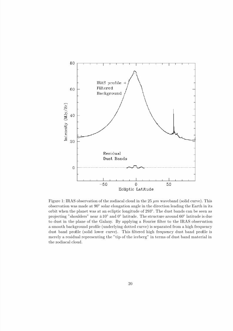
A little over fifteen years ago, the phenomenon of the zodiacal light was attributed to asmooth, lenticular distribution of cometary debris, centered on the Sun, lying in the planeof the ecliptic (see Giese et. al 1986 for a review). However, the launch of IRAS in 1983revolutionized our knowledge of the interplanetary medium. For the first time, brightnessprofiles of the zodiacal cloud became available which clearly showed a level of structure,particularly near the ecliptic, which could not be explained by the previous paradigm.Figure 1 shows such a brightness profile of the zodiacal cloud, along with the results of passing the profile through a fast Fourier filter to isolate the near-ecliptic features. Thesefeatures appear as ‘shoulders’ superimposed on the background emission at roughly ±10,and a ‘cap’ near the ecliptic plane. In the discovery paper, Low et. al (1984) suggest thatthese dust bands are traces of collisional debris within the main asteroid belt, based ona determination of their color temperature. This is an important point: the traditionalsource of the interplanetary dust complex was assumed to be the debris of short periodcomets (Whipple 1967; Dohnanyi 1976). Although asteroid collisions should inject at leastsome material into the cloud, the lack of observational constraints had otherwise made the
contribution of asteroidal material next to impossible to estimate.A dust band is a toroidal distribution of dust particles with common inclinations. The
dust particles themselves are asteroidal collisional debris. Particles in cometary type orbitshave high orbital eccentricities; planetary gravitational perturbations produce large vari-ations in these eccentricities and these variations are coupled to those in the inclinations(Liou et al. 1995). Therefore even if a group of cometary type orbits initally had identicalinclinations, planetary perturbations would disperse those inclinations over a wide range ona timescale of a few precession periods, showing that it is impossible for a comet to producea well defined dust band.
A given asteroid undergoing a collision will break up producing debris according to somesize-frequency distribution. This distribution can be defined by the equation,
n(D) ∼ D2−3q, (1)
where D is the diameter of the particle. For a system in collisional equilibrium, q=11/6(Dohnanyi 1969) and the distribution is dominated by small particles. Assuming the excessvelocities after escape are small compared with the mean orbital speed of an asteroid (15-20km/s), the orbits of individual fragments will be similar as their orbital elements will beonly slightly perturbed from those of the parent asteroid (Davis et al. 1979). Even a smallinitial distribution in relative velocity (10-100 m/s), corresponding to a minor dispersion insemimajor axis ∆a/a (0.1-1%) rapidly produces a ring of material over the parent asteroid’sorbit (102-103 years). Secular precession acts upon the particles’ longitude of ascending nodedue to the effect of Jovian perturbations. To first order,
Ω = − 3GM J a3/2
4R3J
√GM ⊙
1 + 15
8a2
R2J
(2)
where Ω is the longitude of node, M J is Jupiter’s mass, M ⊙ is the Sun’s mass, RJ is themean orbital distance of Jupiter (5.2 AU), a is the semimajor axis of a given particle andG is the gravitational constant (Sykes and Greenberg 1986). The rate of nodal regressionis found from the derivative of the above equation,
∆Ω =9GM J a3
/2
8R3J
√GM ⊙
1 +
35
8
a2
R2J
∆a
a. (3)
4

8/14/2019 The Size-Frequency Distribution of the Zodiacal Cloud- Evidence from the Solar System Dust Bands
http://slidepdf.com/reader/full/the-size-frequency-distribution-of-the-zodiacal-cloud-evidence-from-the-solar 5/46
The time taken to distribute the nodes around the ecliptic to form a dust band is then givenby
∆t =2π
∆Ω . (4)
For a collisional event at 2.2 AU with ejection velocities of 100 m/s, a dust band would
form after approximately 2 x 10⁶
years. Now since particles in inclined orbits spend adisproportionate amount of time at the extremes of their vertical harmonic oscillations, aset of such orbits with randomly distributed nodes will give rise to two apparent bands of particles symmetrically placed above and below the mean plane of the system (Neugebaueret al. 1984). This gives a natural explanation for the ‘shoulders’ on the IRAS profilesat approximately ±10. Similarly, the central ‘cap’ may be simply explained as a lowinclination dust band. Any dispersion in the proper inclinations of the dust particles willlead to the dust band profile appearing broader, with the peak intensity shifted to a lowerlatitude (Dermott et al. 1990, Grogan et al. 1997).
A point of debate in the literature rests on whether the dust bands are equilibrium ornon-equilibrium features. In other words, are the dust bands produced by a gradual grinding
down of asteroid family members, or do they represent regions of random, catastrophicdisruptions in the asteroid belt? The equilibrium model, first discussed by Dermott et al.(1984) and most recently by Grogan et al. (1997), observes that the positions of the dustbands follow the locations of the major Hirayama asteroid families. This would b e thenatural consequence if the local volume density of dust, produced from continual asteroiderosion, followed the local volume density of asteroids. The catastrophic model follows froma discussion of dust band production rates (assuming the random disruption of a smallsingle asteroid of approximately 15km diameter) and dust band lifetimes (material will beremoved by Poynting-Robertson (P-R) drag). Following this logic Sykes and Greenberg(1986) conclude that several dust bands should be visible at any given time. This is inagreement with the IRAS observations and represents the main argument for the non-equilibrium model. The question is an important one to answer, and has implications forthe investigation of the long-term evolution of the asteroid belt. If the equilibrium modelproves correct, then the dust bands can be used as probes of collisional activity within theircorresponding families and ultimately employed to estimate the percentage contribution of asteroidal material to the zodiacal dust complex. If the catastrophic paradigm is correct,then individual dust band features cannot be related to given asteroids in the belt with anyconfidence, and the question of the asteroidal contribution to the cloud will be much moredifficult to unravel.
2 IRAS Observations of the Dust Bands
Dust band structures are not observed independently from the rest of the zodiacal cloud.The IRAS observations consist of a series of line of sight brightness profiles taken throughthe zodiacal cloud as a whole and to study the bands they must somehow be isolated fromthe remainder of the cloud. Various techniques have been employed in the literature for thispurpose. Sykes (1990) uses a boxcar averaging method: this process averages data valuesover a given filter width (latitude bin) and subtracts that average from the central samplevalue. The filter is then shifted by one sample and the process repeated. This has the effectof smoothing the data, and the difference b etween the original data and the smootheddata gives the residuals which are then associated with the dust bands. Reach (1992)
5
8/14/2019 The Size-Frequency Distribution of the Zodiacal Cloud- Evidence from the Solar System Dust Bands
http://slidepdf.com/reader/full/the-size-frequency-distribution-of-the-zodiacal-cloud-evidence-from-the-solar 6/46
and Jones and Rowan-Robinson (1993) assume some empirical form for the backgroundcomponent, and subtract this from the observations to produce residuals which can then beassociated with the dust bands. Finally, Fourier analysis has been employed (Dermott etal. 1986, Sykes 1988, Grogan et al. 1997, Reach et al. 1997) where a smooth low frequencybackground is separated from the high frequency dust band residuals.
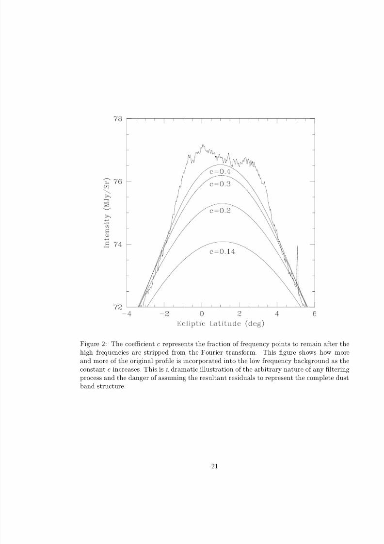
In this paper, the dust band residuals will be obtained by means of a fast Fourierfilter. This filter is sampled at an equal number of points as the number of data p oints inthe brightness profile. The frequency cut-off is defined by a simple coefficient c, a numberwhich varies from 0 to 1 to represent the fraction of frequency points to remain after the highfrequencies are stripped from the Fourier transform. In other words, defining this coefficientequal to 1 would leave the complete Fourier transform intact. Figure 2 demonstrates howmore and more of the original profile is incorporated into the low frequency backgroundas the constant c increases. This is a dramatic illustration of the arbitrary nature of anyfiltering process and the danger of assuming the resultant residuals to represent the completedust band structure.
The viewing geometry of the IRAS spacecraft was ideal for the study of the zodiacalcloud. The Medium Resolution (2’ in scan) Zodiacal Observational History File (ZOHF)consists of 5757 sky brightness profiles, each providing a detailed view of the pole-to-polecloud structure in a given line of sight defined by the ecliptic longitude of Earth, withmost scans being taken at around 90 solar elongation. Towards the end of the survey thesatellite covered elongation angles between 60 and 120, but most of these observationswere contaminated by Galactic emission as the Galactic plane was at this point close tothe ecliptic. The changes in shape and amplitude of the dust band residuals from profile toprofile are caused by a combination of the complex three-dimensional structure of the dustbands themselves and also the observing geometry of the IRAS satellite.
The two primary causes for a change in the line of sight are (1) the longitude of Earthand (2) the solar elongation angle. The changes due to these two parameters are taken tobe independent to first order, allowing a quantitative parameter to be associated with each.
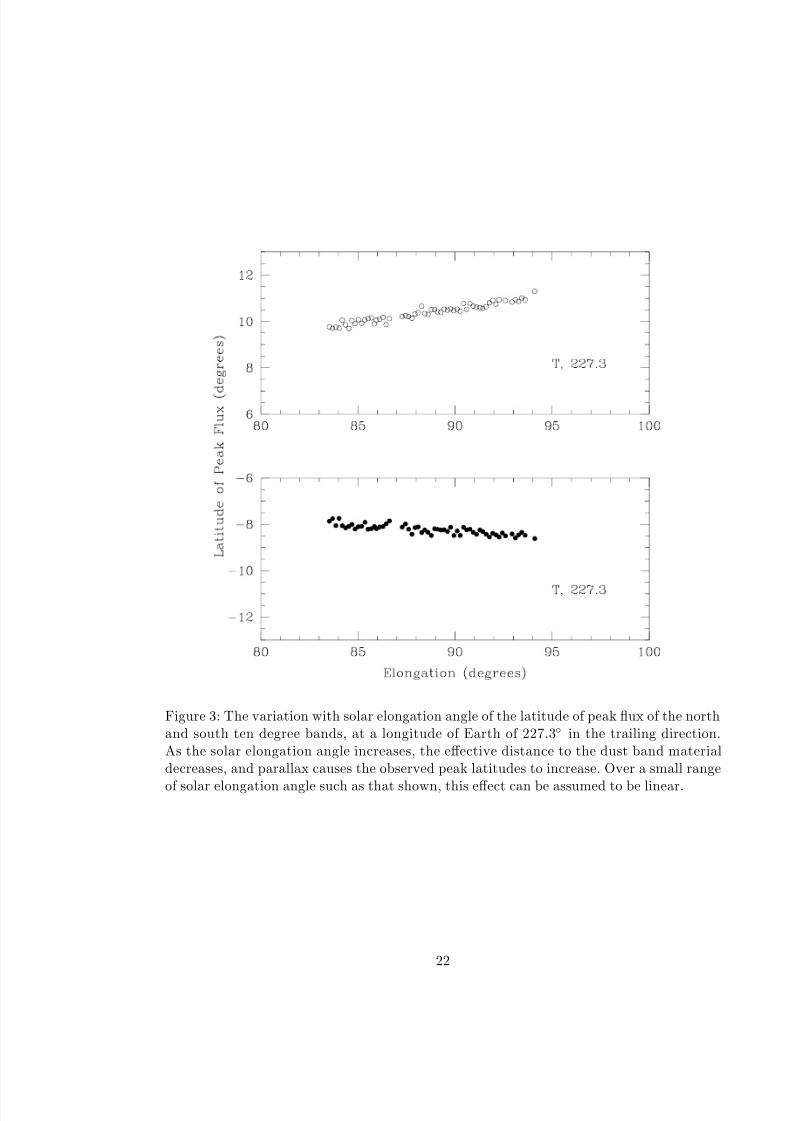
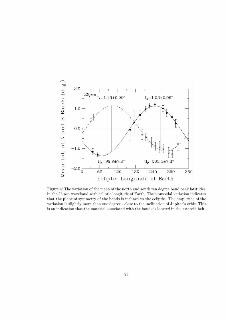
Changes in elongation angle produce a parallax effect: there is a change in the effectivedistance to the bands, and for small changes in elongation angle the effect can be assumedto be linear. The slope dγ/dǫ for the change in peak latitude of the north or south dust bandβ N or β S with elongation angle can be found from a number of scans of a given longitude of Earth with varying solar elongation and this used to normalize the peak latitude that wouldbe observed at a solar elongation of 90 (an example is shown in Figure 3 for a longitudeof Earth of 227.3, trailing direction). Once this has been done, the normalized values of β N and β S may be used to obtain < β >, the mean north/south peak latitude, which maybe plotted as a function of ecliptic longitude of Earth. This is shown in Figure 4 for theten degree band in the 25 µm waveband. The sinusoidal variation indicates that the planeof symmetry of the bands, the plane about which on average the proper inclinations of the
particles precess, is inclined to the ecliptic. This tilt of the plane of symmetry is due tothe secular perturbations of the planets, and its orientation depends on the forced elementsimposed on the dust particles. When viewed from Earth such a plane would appear asa sine curve, its amplitude equal to the inclination of the plane. Also, the displacementfrom the ecliptic will be equal in the trailing and leading directions at the ascending anddescending nodes. Profiles of different longitudes of Earth can now be coadded using theparameters of the sine curve representing the peak latitude of the bands due to their planeof symmetry being inclined to the ecliptic; this effect translates into a lateral shift that canbe positive or negative depending on the longitude of Earth, and a minimum when Earth
6

8/14/2019 The Size-Frequency Distribution of the Zodiacal Cloud- Evidence from the Solar System Dust Bands
http://slidepdf.com/reader/full/the-size-frequency-distribution-of-the-zodiacal-cloud-evidence-from-the-solar 7/46
is at the forced nodes.Individual IRAS scans were Fourier filtered and the dust band residuals coadded in the
above manner to produce several representative profiles around the sky normalized to asolar elongation angle of 90 with noise levels an order of magnitude less than the originalscans. The results of this process for the 12, 25 and 60 µm wavebands, leading and trailing,
are shown in Figures 5-7. The dust band emission peaks in the 25 µm waveband, althoughthe bands are still clearly visible at 12 and 60 µm. The dust bands have a lower amplitudebut similar shape at 12 µm compared to 25 µm, whereas at 60 µm the central band isless prominent with respect to the ten degree band, an effect which is largely due to thefiltering process. These observations contain a wealth of information about the structureof the dust bands; certain aspects, however, deserve special mention. Firstly, there existsa sinusoidal variation in the latitudes of peak brightness of the north and south ten degreeband pair around the sky. This is due to the forced inclinations imposed on the dustband particle orbits by planetary gravitational perturbations as described above. Secondlythere is a clear split in the central band and the amplitudes of each peak vary around thesky. The amplitudes of the north and south ten degree band pair also undergo such avariation except that this variation seems to be out of phase with the variation seen in thecorresponding north and south peaks of the central band. The complex structure revealedby these observations underlines the point that empirical models which attempt the describethe zodiacal cloud as a whole will always fall short in accounting for features such as these,and the problem demands a detailed dynamical treatment.
3 A Physical Model for the Dust Bands
The legacy of the IRAS, COBE and ULYSSES spacecraft is a realization that the zodiacalcloud may consist of five distinct and significant components. These are (1) the asteroidaldust bands (Dermott et al. 1984; Sykes and Greenberg 1986; Reach 1992; Grogan etal. 1997), (2) dust associated with other background (non-family) asteroids, (Dermott etal. 1994a) (3) dust associated with cometary debris (Sykes and Walker 1992; Liou andDermott 1995), (4) the Earth’s resonant ring (Dermott et al 1994b), and (5) interstellardust (Grun et al. 1994; Grogan et al. 1996). It is also possible that a significant proportionof interplanetary dust particles originate in the Kuiper belt (Flynn 1996, Liou et al. 1996).The approach of the Florida group (Dermott et. al) has been to place constraints on theorigin and evolution of material of a given source from both dynamical considerations andobservational data. Given a p ostulated source of particles, the aim is to describe (1) theorbital evolution of these particles, including P-R drag, using equations of motion thatinclude the solar wind, light pressure and planetary gravitational perturbations, and (2)the thermal and optical properties of the particles and their variation with particle size.Once the dust particles and their distribution have been specified along these lines, a line-
of-sight integrator is employed to not only view the model cloud but to reproduce the exactviewing geometry of any particular telescope in any given waveband. The result is a seriesof model profiles which can then be compared with observations.
Amongst the various forces acting upon the dust particles the most obvious is solargravity,
F grav(r) = GMm
r2(5)
where G is the gravitational constant and M is the solar mass. Scattering and absorption of
7
8/14/2019 The Size-Frequency Distribution of the Zodiacal Cloud- Evidence from the Solar System Dust Bands
http://slidepdf.com/reader/full/the-size-frequency-distribution-of-the-zodiacal-cloud-evidence-from-the-solar 8/46
solar radiation by a dust particle involve the transfer of momentum and hence to a radiationpressure directed radially outwards (Burns et al. 1979). For spherical particles radiationpressure takes the value
F rad(r) =SA
cQ pr (6)
where S = L/4πr2
is the radiation flux density at distance r, L is the solar luminosityand Q pr is an efficiency factor averaged over the solar spectrum which can be calculatedusing, for example, Mie theory (Bohren and Huffman, 1983). Radiation pressure is usuallyexpressed as the ratio of its strength to the gravitational attraction, which for sphericalparticles is given by
β =F radF grav
= 5.7 × 10⁻⁵Q pr
ρs(7)
where s is the particle radius and ρ and s are given in cgs units. Roughly speaking,radiation pressure balances gravity for a 1 µm particle. The component of radiation pressuretangential to the particle orbit gives rise to the phenomenon known as Poynting-Robertson(P-R) drag, which results in an evolutionary decrease in both the semi-major axis and
eccentricity of the particle orbit. These changes in the orbital elements can be given byda
dt= −α
2 + 3e2
a(1 − e2)3/2(8)
de
dt= − 5αe
2a2(1 − e2)1/2(9)
di
dt= 0 (10)
where
α =3.35 × 10⁻¹⁰Q pr
s(m)AU 2/yr (11)
(Wyatt and Whipple 1950). The consequence is that the orbit shrinks and circularizes, anda particle in a circular orbit at heliocentric distance r spirals into the Sun in a time
τ pr = 700 s(µm) ρ(g/cm3) r2(AU ) Q pr yrs (12)
This equates to several 104 years for a ‘typical’ particle (10 µm, 2.5 g/cm3, initial r=2 AU).Now consider the motion of dust particles under the effects of planetary gravitational
perturbations. When the eccentricity and inclination are small, the solutions of the La-grangian equations of motion for the eccentricity and pericenter variations may be com-pletely decoupled from the inclination and node variations. These pairs of elements havesimple vectorial representations and may be decomposed into components known as the
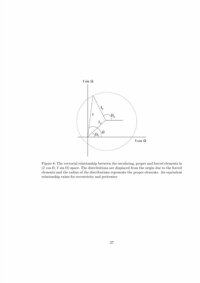
proper elements and the forced elements of the orbit. The proper elements represent thestable long-term averages that remain after removal of planetary perturbations. The varia-tions due to these perturbations are the forced elements, which can themselves be separatedinto three categories: (1) secular (long period) perturbations; (2) resonant (short period)perturbations; (3) transient (scattering) perturbations. These perturbations acting on asmall body in orbit about the Sun precess the node and pericenter and over sufficiently longintervals the distributions of these elements become essentially random. Figure 8 shows aschematic of the vectorial relationship between the total (osculating) elements (I , Ω), theproper elements (I p, Ω p) and the forced elements (I f , Ωf ) in (I cos Ω, I sin Ω) space. The
8
8/14/2019 The Size-Frequency Distribution of the Zodiacal Cloud- Evidence from the Solar System Dust Bands
http://slidepdf.com/reader/full/the-size-frequency-distribution-of-the-zodiacal-cloud-evidence-from-the-solar 9/46
distribution is displaced from the origin due to the forced elements and the radius of thedistribution represents the proper elements. An equivalent relationship exists for eccen-tricity and pericenter. Figures 9 and 10 show the evolution of 249 Koronis dust particlesmigrating from the asteroid belt toward the Sun (Kortenkamp and Dermott 1998). Secularperturbations, primarily from Jupiter and Saturn, vary with time and semi-major axis and
act to change the forced elements of the distribution as the wave migrates into the innerSolar System. The orbital eccentricities also decay due to P-R drag and solar wind drag.Dermott et al. (1984) were the first to suggest that the Solar System dust bands may
originate in the three prominent Hirayama asteroid families (Eos, Themis and Koronis).To confirm their hypothesis of the asteroidal origin of the dust bands, and to facilitate theinvestigation of the zodiacal cloud in general, SIMUL, a three-dimensional numerical modelwas constructed (Dermott et al. 1988). The basic ideas and assumptions behind SIMULare as follows.
1. A cloud is represented by a large number of dust particle orbits. The total cross-sectional area of the cloud is divided equally among all the orbits.
2. The orbital elements of the dust particle orbits in the cloud can be decomposed intoproper and forced vectorial components. When inclination and eccentricity are low,as is typically the case for asteroidal type orbits, at any given time the forced elementsare independent of the proper elements and depend only on the semimajor axis andthe particle size.
3. As a first approximation, the dust particles in the cloud produced by asteroid familieshave the same mean proper elements as those of the parent bodies, although theGaussian distribution of these elements is a free parameter.
4. The forced elements as a function of semimajor axis are calculated using secularperturbation theory via direct numerical integrations, as outlined above.
5. Along each of the orbits, particles are distributed according to Kepler’s Law. Oncethe spatial distribution of the orbits is specified, space is divided into a sufficientlylarge number of ordered cells and then every orbit is investigated for all the possiblecross-sectional area contributions to each of the space cells. The model generates alarge three-dimensional array which serves to describe the spatial distribution of theeffective cross-sectional area.
6. The viewing geometry of any telescope can b e reproduced exactly by calculating theSun-Earth distance and ecliptic longitude of Earth at the observing time and settingup appropriate coordinate systems. In this way, IRAS-type brightness profiles can becreated and compared with the observed profiles.
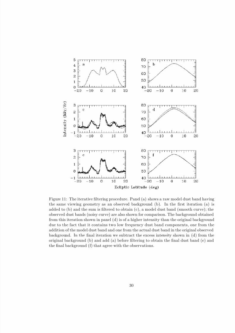
In order to compare the results of the SIMUL modeling algorithm with the IRAS ob-servations, the filtering problem - the fact that a substantial percentage of the dust bandsignal is indistinguishable from the background - must b e addressed. An iterative process(Dermott et al. 1994a, Grogan et al. 1997) is used to determine the low-frequency com-ponent of the dust band and therefore bypass this filtering problem. Figure 11 shows howthis is achieved. Panel (a) shows a raw model dust band having the same viewing geometryas an observed background, produced by filtering off the high-frequency dust band com-ponent. In the first iteration (a) is added to (b) and the sum is filtered to obtain (c), a
9

8/14/2019 The Size-Frequency Distribution of the Zodiacal Cloud- Evidence from the Solar System Dust Bands
http://slidepdf.com/reader/full/the-size-frequency-distribution-of-the-zodiacal-cloud-evidence-from-the-solar 10/46
filtered model dust band (smooth curve) - the observed dust bands (noisy curve) are alsoplotted for comparison. The background obtained from this iteration, shown in panel (d)is of a higher intensity than the original background due to the fact that it contains twolow-frequency dust band components, one from the addition of the model dust band andone from the actual dust band in the original observed background (the high frequency
component of which was removed in the creation of the observed background). In otherwords, the difference between these two backgrounds gives the extent of the low-frequencydust band component. In the final iteration we subtract the excess intensity shown in panel(d) from the original background (b) and add (a) before filtering to obtain the final dustband model (e) and the final background (f) that agree with the observations. Thus, byusing the same filter in the modeling process that we use to define the observed dust bands,and iterating, we are able to bypass the arbitrary divide associated with the filter.
4 Results
This work differs from our previous modeling of the dust bands (Grogan et al. 1997)
in that our models include a size-frequency distribution, rather than being composed of particles of a single size. This is critical in our efforts to provide a model of the dust bandsthat can match the IRAS observations in multiple wavebands. Particles ranging in sizefrom 1 to 100 µm are included, each of which are assumed to be Mie spheres composedof astronomical silicate (Draine and Lee 1984). The lower end cut-off is determined bythe fact that contribution to the thermal emission from particles smaller than this size isnegligible. The upper cut-off follows from the fact that in the zodiacal cloud, the P-R draglifetime is comparable to the collisional lifetime for a particle of about this size (Leinert andGrun 1990). However, the inclusion of a wide range of particle sizes can only b e achievedwith an understanding of their dynamical history, so that their orbital distributions can beproperly described in the SIMUL algorithm. This is achieved using the RADAU fifteenthorder integrator program with variable time steps taken at Gauss-Radau spacing (Everhart1985), with which we perform direct numerical integration of the full equations of motion of interplanetary dust particles (IDPs) of various sizes. Our simulations include seven planets(Mercury and Pluto excluded) and account for both P-R drag and solar wind drag. Theaverage force due to the solar wind drag is taken to be 30% of the P-R drag force, varyingwith the 11-year solar cycle from 20% to 40% (Gustafson 1994). In this way we are ableto build a description of both the proper and forced elements of the particles and theirvariation with heliocentric distance from their simple vectorial relationship shown in Figure8. Because the forced elements vary as a function not only of semi-major axis but also of time, each wave of particles (as shown in Figures 9 and 10) is started at different timesin the past, such that when the waves reach the present they span the full range of semi-major axis from the asteroid belt into the Sun. In this way a snapshot of the present day
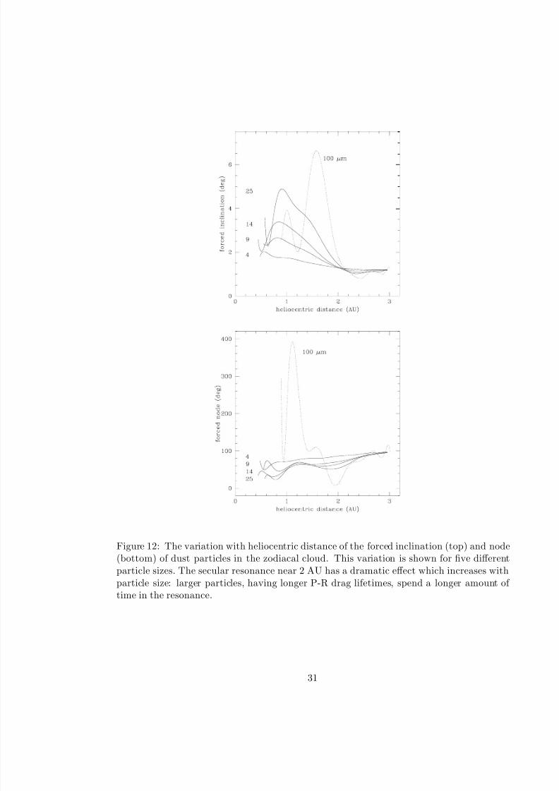
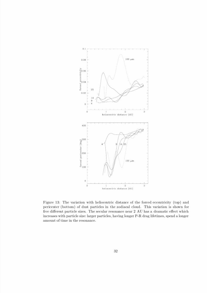
forced element distribution is constructed. Figure 12 shows the variation with heliocentricdistance of the forced inclination (top) and forced longitude of ascending node (bottom) of 4, 9, 14, 25 and 100 µm diameter IDPs in the zodiacal cloud. As the particle size increases,its P-R drag lifetime increases and it therefore spends longer in secular resonances near theinner edge of the asteroid belt. This causes the forced inclination of a 100 micron diameterparticle to approach 6 interior to 2 AU. An equivalent diagram for the forced eccentricityand forced pericenter is shown in Figure 13.
Dust band models are produced via SIMUL in the following manner.
10

8/14/2019 The Size-Frequency Distribution of the Zodiacal Cloud- Evidence from the Solar System Dust Bands
http://slidepdf.com/reader/full/the-size-frequency-distribution-of-the-zodiacal-cloud-evidence-from-the-solar 11/46
1. A model to account for the central band is created by using two distributions of orbitshaving mean semi-major axis, proper eccentricity, proper inclination and dispersionsequal to those found in the Themis and Koronis families. The proper elements foundfrom the numerical integrations are added vectorially to find the osculating orbitalelements, and the material is distributed into the inner Solar System as far as 2 AU
according to P-R drag (a 1/rγ
, γ = 1.0 distribution). The size-frequency distributionof material in the observed dust band is investigated by varying the size-frequencyindex q of particles in the model.
2. A model to account for the ten degree band is created from Eos type orbits, in thattheir mean semi-major axis and eccentricity are equal to those found in the Eosfamilies. However, in order to improve upon previous modeling of the ten degreeband the mean proper inclination of the distribution was allowed to vary within therange of proper inclinations found in the Eos family. A best fit was found at a meanproper inclination of 9.35 with a dispersion of 1.5. Again, the proper elements areadded vectorially, the material distributed into the inner Solar System as far as 2 AU,and a size-frequency distribution applied.
3. We do not create a model for the zodiacal background but instead add the modeldust band profiles to the observed background obtained from applying the Fourierfilter to the corresponding raw IRAS observation. The total is then filtered usingthe iterative procedure described above so that the resultant model residual can bedirectly compared with the observed dust bands. For a given size-frequency index q,the total surface area of material associated with the model bands is adjusted untilthe amplitudes of the 25 µm model dust bands matches the 25 µm observations; qcan then be varied until a single model provides a match in amplitude to the 12, 25and 60 µm observations simultaneously.
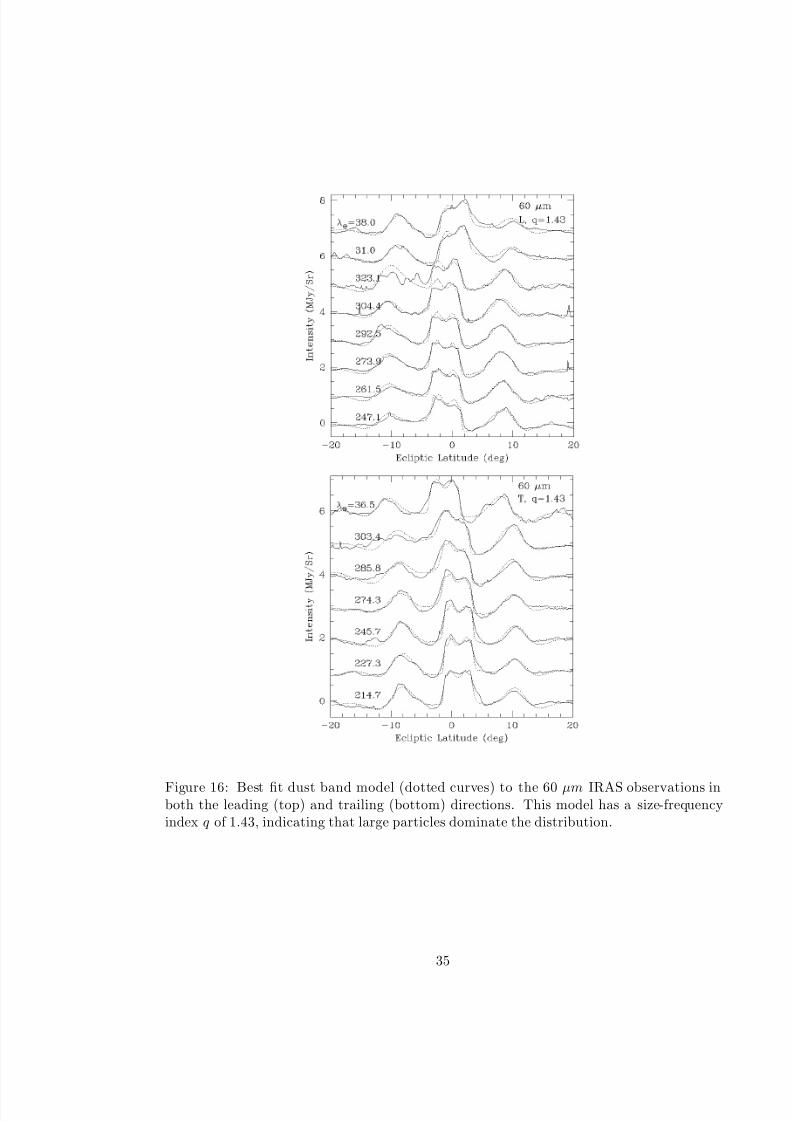
Figures 14-16 show the best results of our modeling, comparing the dust band obser-
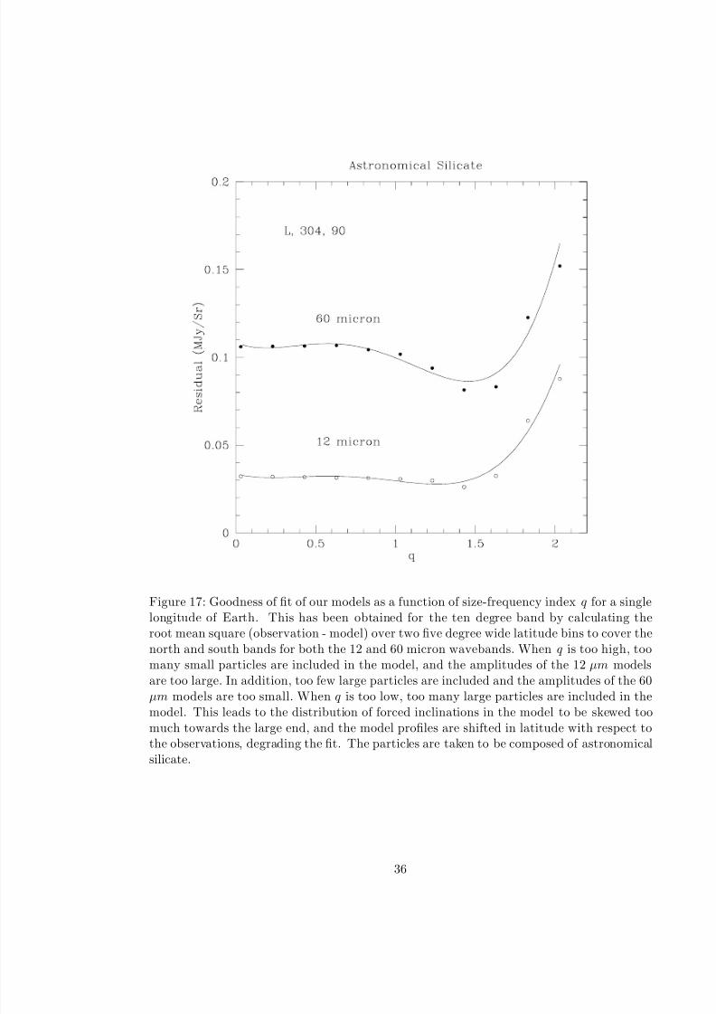
vations (solid curves) to the dust band models (dotted curves) in the 12, 25 and 60 µmwavebands. The models were constructed as described above, and have a size-frequencyindex q equal to 1.43. Large particles dominate this distribution. Table 1 lists the param-eters used in the model components. The amplitudes in all wavebands are well matched,and the shapes of the dust band models describe the variation in shape of the observationsaround the sky very well. Figure 17 shows how the goodness of fit of our models changes asa function of size-frequency index q for a single longitude of Earth. This has been obtainedfor the ten degree band by calculating the root mean square (observation - model) over twofive degree wide latitude bins to cover the north and south bands for both the 12 and 60micron wavebands. In essence, the wavebands act as filters through which different particlesizes in the cloud are seen. The 12 µm waveband preferentially detects emission from the
smaller particles, and the 60 µm waveband preferentially detects emission from the largerparticles. Therefore,
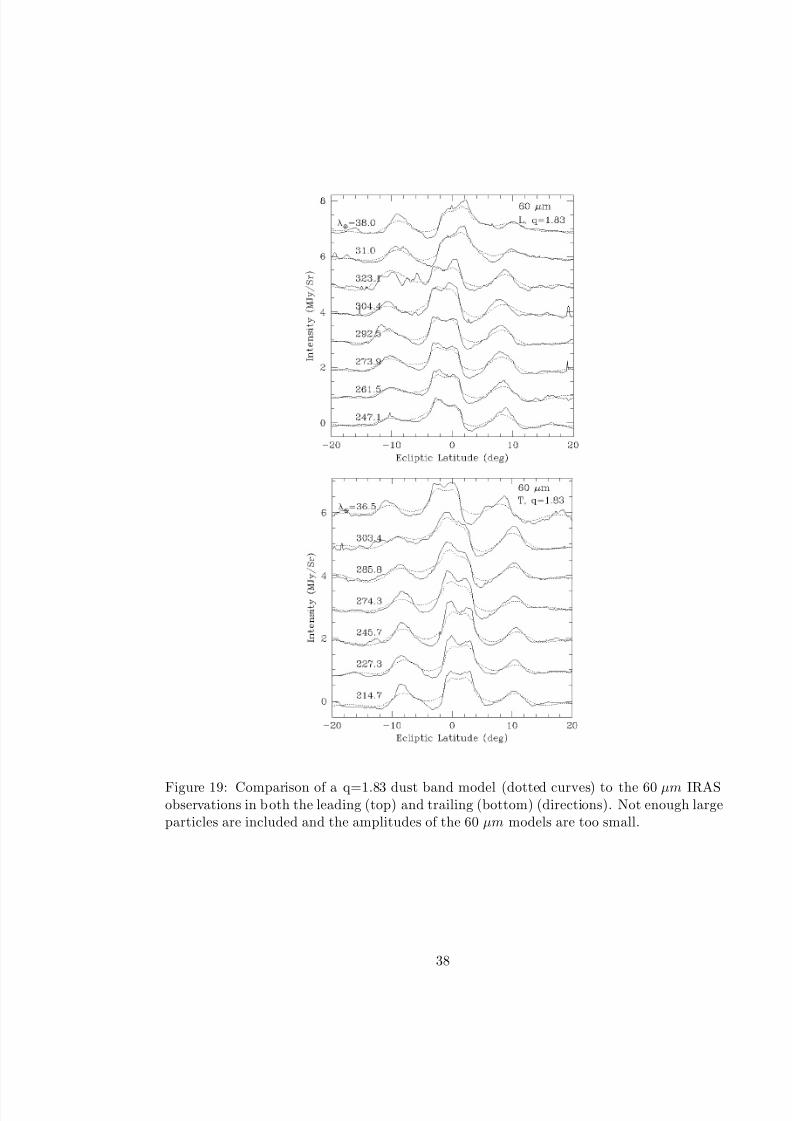
1. When q is too high, too many small particles are included in the model, and theampitudes of the 12 µm models are too large. In addition, too few large particles areincluded and the amplitudes of the 60 µm models are too small. This effect can beseen in Figures 18-19, in which dust band models have been produced with q=1.83,appropriate for a system in collisional equilibrium.
11
8/14/2019 The Size-Frequency Distribution of the Zodiacal Cloud- Evidence from the Solar System Dust Bands
http://slidepdf.com/reader/full/the-size-frequency-distribution-of-the-zodiacal-cloud-evidence-from-the-solar 12/46
2. When q is too low, too many large particles are included in the model. This leads tothe distribution of forced inclinations in the model to be skewed too much towardsthe large end, and the model profiles are shifted in latitude with respect to the obser-vations, degrading the fit. This effect is much smaller than the amplitude effect forhigh q, and will only be properly quantified when a fuller description of the action of
large particles at the 2 AU secular resonance has been produced.A clear result is that a high size-frequency index q, in which small particles dominate,
fails to account for the observations of the Solar System dust bands. This index has tobe reduced to the point where large particles dominate the distribution. This is consistentwith the cratering record on the LDEF satellite, shown in Figure 20, which suggests a q of approximately 1.15 at Earth and a peak in the particle diameter at around 100-200 micron.Since the Fourier filter preferentially isolates material exterior to the 2 AU secular resonance(in the inner Solar System the dust band material is dispersed into the background clouddue to the action of secular resonances), our results are more indicative of the size-frequencyindex of dust in the asteroid belt. We do not mean to claim that the size-frequency indexq is a constant throughout the main-belt: the true nature of the distribution will be a
complex function of dust production rates, P-R drag rates, collisional lifetimes and thenature of particle-particle collisions. Consequently, the size distribution will presumablybe some function of heliocentric distance. However, in describing in main belt region as awhole, we do claim that large particles appear to dominate the dust band emission oversmall particles.
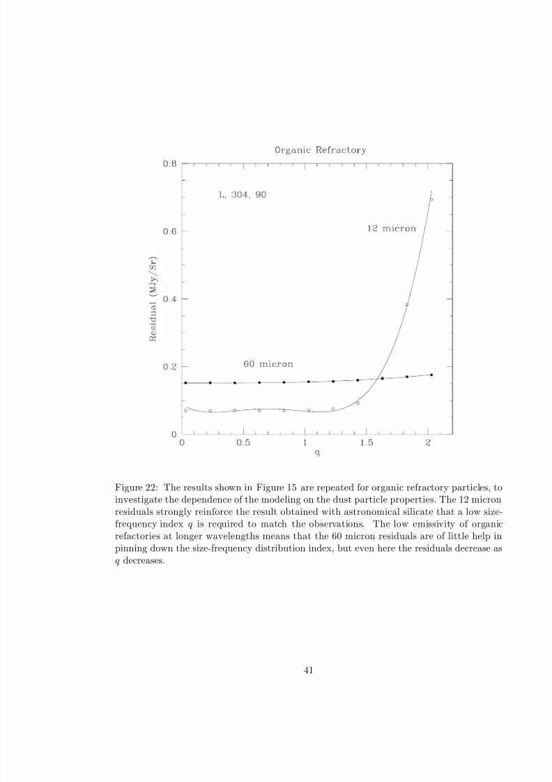
One concern that must be addressed is the possibility that the observed relative ampli-tudes of the dust band material are driven by the optical properties of the dust particles,and not the size-frequency index. For this reason, we have repeated the modeling processassuming the particles to be made of organic refactory material (Li and Greenberg 1997).Figure 21 shows the variation with wavelength and particle diameter of the absorptionefficiencies of both astronomical silicate (top) and organic refractory material (bottom),
calculated using Mie theory. One striking difference between the two, particularly relevantfor this discussion, is that emission at longer wavelengths for large particles is highly at-tenuated for the organic refractory material compared to the astronomical silicates. Figure22 shows how the residuals obtained in the modeling process are affected by the change inthe composition of the dust particle. The 12 micron residuals strongly reinforce the resultobtained with astronomical silicate that a low size-frequency index q is required to matchthe observations. The evidence at 60 micron is less clear, where we are hindered by the lowemissivity of this material at longer wavelengths for larger particles. Even so, the residualsare decreasing with decreasing q. The consistent picture is that the dust band distributionis dominated by particles at the large end of the size range.
5 Discussion
The results presented in this paper improve upon those reported in a previous paper (Groganet al. 1997), particularly in regard to the ten degree band associated with the Eos family.In order for a dust band model to match the observations, it needs to fit both the latitude of peak flux (driven by the mean proper inclination of the particles) and the width of the dustband feature (a function of the dispersion in proper inclinations). Previously, the dispersionin proper inclinations of the Eos dust particles was reported at a relatively high 2.5, whichminimized the residuals while the mean proper inclination of the particles was fixed at the
12
8/14/2019 The Size-Frequency Distribution of the Zodiacal Cloud- Evidence from the Solar System Dust Bands
http://slidepdf.com/reader/full/the-size-frequency-distribution-of-the-zodiacal-cloud-evidence-from-the-solar 13/46
mean proper inclination of the Eos asteroid family. In this paper, smaller residuals are foundwhen the mean proper inclination of the particles is allowed to float as a free parameter;the best fit then corresponds to a mean proper inclination of 9.35 and a dispersion of only1.5.
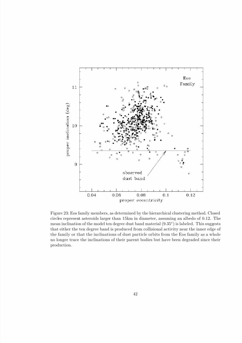
Figure 23 shows the members of the Eos asteroid family in (e,i) space as determined
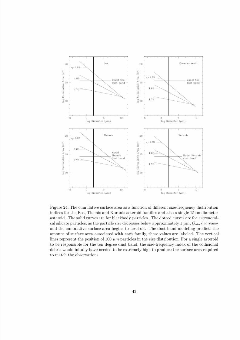
by the hierarchical clustering method (Zappala et al. 1995). Shown on this diagram is theposition of the mean proper inclination of the ten degree band model. The consequence isthat the ten degree dust band material is not tracing the orbital element space of the Eosfamily as a whole, as would perhaps be expected from the equilibrium model. Either thecollisional activity is occurring near the inner edge of the Eos family, or the inclinationsof dust particle orbits originating from the Eos family as a whole no longer trace the in-clinations of their parent b odies but have been degraded since their production. If somemechanism was degrading the dust particle orbits it would presumably apply to particlesfrom all sources, but may be more easily observed within the Eos family owing to its highinclination. Trulsen and Wikan (1980) have suggested based on their numerical simulationsthat the combined influence of P-R drag and collisions acts to decrease both the mean ec-centricity and inclination of dust particle orbits. This subject is however open to debate; thenature of collisions between interplanetary dust particles is still poorly understood. Figure24 shows the cumulative surface area as a function of different size-frequency distrubtionindices for the Eos, Themis and Koronis families and also a single 15km diameter asteroid.At first this appears to contradict our result that a low q of around 1.43 is needed to modelthe dust bands. However, the diagram is set up such that size-frequency distribution isconstant from the source point all the way down to the smallest IDPs, which we know isnot the case since P-R drag will act to preferentially remove the small particles. In reality,the size-frequency distribution will change from the large to the small end of the distribu-tion, and will also be a function of heliocentric distance. The diagram does suggest that fora single asteroid to be responsible for the ten degree dust band, the size-frequency indexof the collisional debris would initially have needed to be extremely high to produce the
surface area required to match the observations.The justification of cutting off the distribution of dust band material at 2 AU is essen-
tially given by Figure 12. As the particles move out of the asteroid belt the action of thesecular resonance disperses them into the background cloud, an effect which is more markedas the particle size increases. For this reason the Fourier filter is particularly sensitive tomaterial located in the asteroid belt, and models that confine the material to the asteroidbelt match the observations very well. In the future, our models will populate the innerSolar System as well as the main-belt region, but to do this properly we will have to:
1. Investigate the dynamical history of a much greater number of particle sizes than thefive sizes we have considered so far in order to properly account for their behavior atthe 2 AU secular resonance;
2. Take into account collisional processes: larger particles will have shorter collisionallifetimes compared to their P-R drag lifetimes and will therefore not penetrate as farinto the inner Solar System. Each distribution of orbits of a given particle size willtherefore have a natural inner edge defined by the lifetime of the particles in the cloud.
However, we can obtain an estimate for the dust band contribution to the zodaical cloudas a whole by simply extending our best fit dust band models to populate the inner SolarSystem. The distribution of orbits obtained in this manner will not be exactly correct, due
13
8/14/2019 The Size-Frequency Distribution of the Zodiacal Cloud- Evidence from the Solar System Dust Bands
http://slidepdf.com/reader/full/the-size-frequency-distribution-of-the-zodiacal-cloud-evidence-from-the-solar 14/46
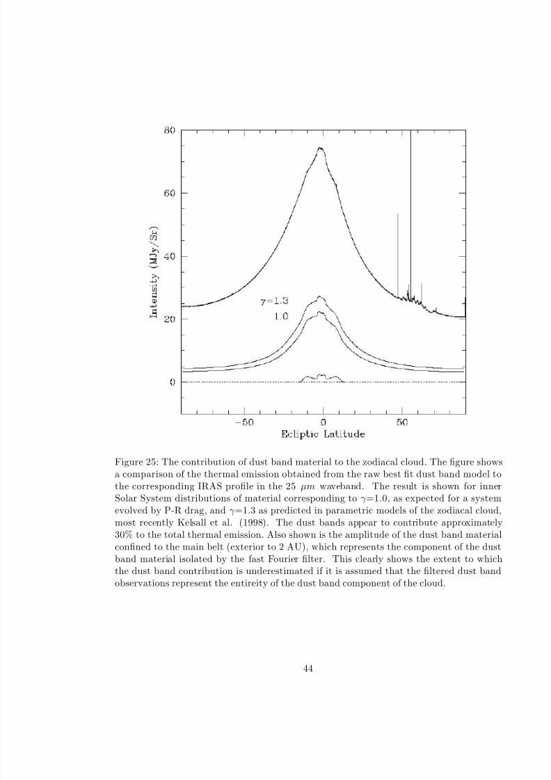
to our insufficient treatment of the secular resonance, but will still be reasonably accuratein terms of the total surface area associated with the dust bands. Figure 25 comparesthe thermal emission obtained from this raw dust band model to the corresponding IRASprofile in the 25 µm waveband. The result is shown for inner Solar System distributions of material corresponding to γ =1.0, as expected for a system evolved by P-R drag, and γ =1.3
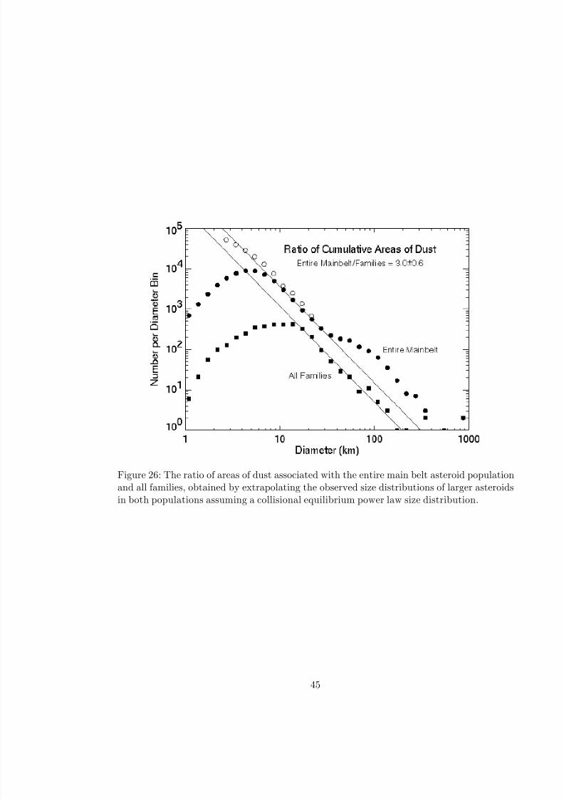
as predicted in parametric models of the zodiacal cloud, most recently Kelsall et al. (1998).The dust bands appear to contribute approximately 30% to the total thermal emission. Alsoshown is the amplitude of the dust band material confined to the main belt (exterior to 2AU), which represents the component of the dust band material isolated by the fast Fourierfilter. This clearly shows the extent to which the dust band contribution is underestimatedif it is assumed that the filtered dust band observations represent the entirety of the dustband component of the cloud. Figure 26 shows the ratio of areas of material associated withthe entire main belt asteroid population and all families, for asteroid diameters greater than1 km. The best fit lines have a slope corresponding to a size-frequency index q = 1.795.This diagram can be used to estimate the total contribution of main belt asteroid collisionsto the dust in the zodiacal cloud, by extrapolating the observed size distributions of largerasteroids in both populations assuming a collisional equilibrium power law size distribution.The result is that the main belt asteroid population contributes approximately three timesthe dust area of the Hirayama families alone, and the total asteroidal contribution to thezodiacal cloud could account for almost the entireity of the interplanetary dust complex.In reality, evolved size distributions are more complex than simple power laws (Durdaet al. 1998) and the size distribution of individual asteroid families likely preserve somesignatures of the original fragmentation events from which they were formed. However,small dust-size particles and their immediate parent bodies have collisional lifetimes in themain belt that are considerably shorter than the age of the Solar System or the majorasteroid families. Thus the dust size distributions associated with both the backgroundmain belt and family asteroids may well be considered to have achieved an equilibriumstate, with total areas related to the equivalent volumes of the original source bodies in
each population. An alternative, and perhaps more satisfactory, approach to obtainingthe total asteroidal contribution to the zodiacal cloud will be to apply our methods to themain-belt asteroid population in the same way we have investigated the dust bands. Thisis the subject of a future paper.
The origin of the large dispersion in proper inclination (1.5) required to successfullymodel the ten degree band, in rough agreement with the 1.4 found by Sykes (1990) andthe 2 found by Reach et al. (1997), remains unclear. Dispersion in inclination due to theLorentz force is expected to behave such that the root mean square of the dispersion willincrease with the square root of the distance traveled, and will be inversely proportional tothe cube of the radius of the particle (Leinert and Grun 1990). Morfill and Grun (1979)report a value of only 0.3 for a particle of 1 µm radius by the time it has spiraled in
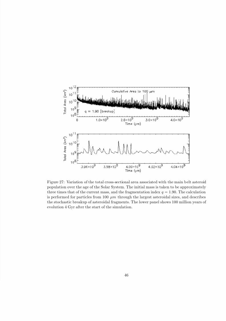
to 1 AU from the asteroid belt after 3000 years, with that expected for a 100 micronparticle to be significantly less. Subsequent treatments by Consomagno (1979), Barge etal. (1982) and Wallis and Hassan (1985) differ by more than an order of magnitude dueto the lack of detailed knowledge of the magnetic field structure. A more likely source of the dispersion is simply the action of the secular resonance at 2 AU. However, this leavesopen the question of why a large dispersion is required to model the ten degree band, andonly the small dispersion of the Themis and Koronis families is required to successfullyreproduce the central band observations. One answer may be that the emission associatedwith the central band is due to relatively recent collisions within these families. Figure 27
14
8/14/2019 The Size-Frequency Distribution of the Zodiacal Cloud- Evidence from the Solar System Dust Bands
http://slidepdf.com/reader/full/the-size-frequency-distribution-of-the-zodiacal-cloud-evidence-from-the-solar 15/46
shows the variation with time of the total cross-sectional area associated with the main beltand describes the stochastic breakup of asteroidal fragments. This numerical approach todescribing the collisional evolution of the asteroid belt is detailed by Durda and Dermott(1997). The initial main belt mass is taken to be approximately three times greater thanthe present mass (Durda et al. 1998); this population evolves after 4.5 Gyr to resemble
the current main belt. The calculation is performed for particles from 100 µm through thelargest asteroidal sizes, with a fragmentation index q = 1.90. The dust production ratein the main asteroid belt becomes more stochastic with time following a relatively smoothdecrease in area as the small particles are created directly from the breakup of the parentbody are destroyed. The spikes in the dust production are due to the breakup of small tointermediate size asteroids. Therefore while the observable volume of a family may decayat a fairly constant and well-defined rate, the total area of dust associated with the familyduring that time may fluctuate by an order of magnitude or more.
We have shown in this paper how the Solar System dust bands can be investigated andused as a tool for addressing fundamental questions about the nature of the zodiacal cloudand the origin of the material from which it is composed. A key component of this processhas been the realization that large particles play a dominating role in the structure of thecloud and that their dynamical histories need to be included in any physically motivatedmodel. In the future we will extend our knowledge of the dust dynamics to a wider range of particle sizes, and address the main-belt contribution as well as the dust band componenton the way to our ultimate goal of providing a global model for the zodiacal emission.
15
8/14/2019 The Size-Frequency Distribution of the Zodiacal Cloud- Evidence from the Solar System Dust Bands
http://slidepdf.com/reader/full/the-size-frequency-distribution-of-the-zodiacal-cloud-evidence-from-the-solar 16/46
References
Barge, P., Pellat, R. and Millet, I. 1982. Diffusion of Keplarian motionsby a stochastic force. II. Lorentz scattering of interplanetary dusts. Astron.
Astrophys. 115, 8-19.
Bohren, C.F. and Huffman, D.R. 1983. Absorption and Scattering of Light by Small Particles, Wiley, New York.
Burns, J.A., Lamy, P.L. and Soter, S. 1979. Radiation Forces on SmallParticles in the Solar System. Icarus 40, 1-48.
Consomagno, G. 1979. Lorentz scattering of interplanetary dust. Icarus 38,398-410.
Davis, D.R., Chapman, C.R., Greenberg, R., Weidenschilling, S.J.
and Harris, A.W. 1979. Collisional evolution of asteroids. In Asteroids, ed.T. Gehrels, 528-557. Univ. of Arizona Press, Tuscon.
Dermott, S.F., Nicholson, P.D., Burns, J.A. and Houck, J.R. 1984.Origin of the Solar System dust bands discovered by IRAS. Nature 312, 505-509.
Dermott, S.F., Nicholson, P.D. and Wolven, B. 1986. Preliminary Anal-ysis of the IRAS Solar System Dust Data. In Asteroids, Comets, Meteors II ,eds. C.-I. Lagerkvist, B.A. Lindblad, H. Lundstedt and H. Rickman, 583-594,Reprocentralen HSC, Uppsala.
Dermott, S.F., Nicholson, P.D., Kim, Y., Wolven, B. and Tedesco,
E.F 1988. The Impact of IRAS on Asteroidal Science. In Comets to Cosmology ,ed. A. Lawrence, 3-18. Springer-Verlag, Berlin.
Dermott, S.F., Nicholson, P.D., Gomes, R.S. and Malhotra, R. 1990.Modeling the IRAS Solar System dust bands. Adv. Space Res. 10(3), 171-180.
Dermott, S.F., Durda, D.D., Gustafson, B.A.S., Jayaraman, S., Liou,
J.C. and Xu, Y-L. 1994a. Zodiacal Dust Bands. In Asteroids, Comets, Me-
teors 1993 , eds. A. Milani, M. Martini and A. Cellino, 127-142. Kluwer, Dor-drecht.
Dermott, S.F., Jayaraman, S., Xu, Y-L., Gustafson, B.A.S. and Liou,
J.C. 1994b. A circumsolar ring of asteroidal dust in resonant lock with theEarth. Nature 369, 719-723.
Dohnanyi, J.S. 1969. Collisional model of asteroids and their debris. J. Geo-
phys. Res. 74, 2531-2554.
Dohnanyi, J.S. 1976. Sources of interplanetary dust, asteroids. In Interplane-
tary Dust and Zodiacal Light, Lecture Notes in Physics Vol. 48 , eds. H. Elsasserand H. Fechtig, 187-205. Springer, Berlin.
Draine, B.T. and Lee, H.M. 1984. Optical properties of interstellar graphiteand silicate grains. Ap.J 285, 89-108.
16
8/14/2019 The Size-Frequency Distribution of the Zodiacal Cloud- Evidence from the Solar System Dust Bands
http://slidepdf.com/reader/full/the-size-frequency-distribution-of-the-zodiacal-cloud-evidence-from-the-solar 17/46
Durda, D.D. and Dermott, S.F. 1997. The Collisional Evolution of theAsteroid Belt and Its Contribution to the Zodiacal Cloud. Icarus 130, 140-164.
Durda, D.D., Greenberg, R. and Jedicke, R. 1998. Collisional Modelsand Scaling Laws: A New Interpretation of the Shape of the Main-Belt AsteroidSize Distribution. Icarus 135, 431-440.
Everhart, E. 1985. An efficient integrator that uses Gauss-Radau spacings.In Dynamics of Comets, eds. A. Carusi and G.B. Valsecchi, 185-202. Reidel,Dordrecht.
Flynn, G.J. 1996. Collisions in the Kuiper Belt and the Production of Inter-planetary Dust Particles. Meteoritics and Planet. Sci. 31, A45.
Giese, R.H., Kneissel, B. and Rittich, U. 1986. Three-dimensional zodi-acal cloud, a comparative study. Icarus 68, 395-411.
Grogan, K., Dermott, S.F. and Gustafson, B.A.S. 1996. An Estimation
of the Interstellar Contribution to the Zodiacal Thermal Emission. Ap.J 472,812-817.
Grogan, K., Dermott, S.F., Jayaraman, S. and Xu, Y-L. 1997. Originof the ten degree dust bands. Planet. Space Sci. 45, 1657-1665.
Grun, E., Gustafson, B.A.S., Mann, I., Baguhl, M., Morfill, G.E.,
Staubach, P., Taylor, A. and Zook, H.A. 1994. Interstellar Dust in theHeliosphere. Astron. Astrophys. 286, 915-924.
Gustafson, B.A.S. 1994. Physics of zodiacal dust. Ann. Rev. Earth Planet.
Sci. 22, 553-595.
Jones, M.H. and Rowan-Robinson, M. 1993. A physical model for the IRASzodiacal dust bands. MNRAS 264, 237-247.
Kelsall, T., Weiland, J.L., Franz, B.A., Reach, W.T., Arendt, R.G.,
Dwek, E., Freudenreich, H.T., Hauser, M.G., Moseley, S.H., Ode-
gard, N.P., Silverberg, R.F. and Wright E.L. 1998. The COBE DiffuseInfrared Background Experiment Search for the Cosmic Infrared Background.II. Model of the Interplanetary Dust Cloud. Ap.J 508, 44-73.
Kortenkamp, S.J. and Dermott, S.F. 1998. Accretion of InterplanetaryDust Particles by the Earth. Icarus 135, 469-495.
Leinert, C. and Grun, E. 1990. Interplanetary Dust. In Space and So-lar Physics, Vol. 20, Physics and Chemistry in Space: Physics of the Inner
Heliosphere I , eds. R. Schween and E. Marsch, 207-275. Springer, Berlin.
Li, A. and Greenberg, J.M. 1997. A unified model of interstellar dust.Astron. Astrophys. 331, 566-584.
Liou, J.C., Dermott, S.F. and Xu, Y-L. 1995. The contribution of cometarydust to the zodiacal cloud. Planet. Space Sci. 43, 717-722.
17
8/14/2019 The Size-Frequency Distribution of the Zodiacal Cloud- Evidence from the Solar System Dust Bands
http://slidepdf.com/reader/full/the-size-frequency-distribution-of-the-zodiacal-cloud-evidence-from-the-solar 18/46
Liou, J.C., Zook, H.A. and Dermott, S.F. 1996. Kuiper Belt Dust Grainsas a Source of Interplanetary Dust Particles. Icarus 124, 429-440.
Low, F.J., Beintema, D.A., Gautier, T.N., Gillet, F.C., Beichmann,
C.A., Neugebauer, G., Young, E., Aumann, H.H., Boggess, N., Emer-
son, J.P., Habing, H.J., Hauser, M.G., Houck, J.R., Rowan-Robinson,
M., Soifer, B.T., Walker, R.G. and Wesselius, P.R. 1984. Infrared Cir-rus: New Components of the Extended Infrared Emission. Ap.J 278, L19-L22.
Morfill, G.E. and Grun, E. 1979. The motion of charged dust particlesin interplanetary space. I. The zodiacal dust cloud. Planet. Space Sci. 27,1269-1282.
Neugebauer, G., Beichman, C.A., Soifer, B.T., Aumann, H.H., Chester,
T.J., Gautier, T.N., Gillett, F.C., Hauser, M.G., Houck, J.R., Lons-
dale, C.J., Low, F.J. and Young, E.T. 1984. Early results from the infraredastronomical satellite. Science 224, 14-21.
Reach, W.T. 1992. Zodiacal Emission III. Dust Near The Asteroid Belt. Ap.J 392, 289-299.
Reach, W.T., Franz, B.A. and Weiland, J.L. 1997. The Three-DimensionalStructure of the Zodiacal Dust Bands. Icarus 127, 461-484.
Sykes, M.V. 1988. IRAS Observations of Extended Zodiacal Structures. Ap.J
334, L55-L58.
Sykes, M.V. 1990. Zodiacal Dust Bands: Their Relation to Asteroid Families.Icarus 84, 267-289.
Sykes, M.V. and Greenberg, R. 1986. The Formation and Origin of theIRAS Zodiacal Dust Bands as a Consequence of Single Collisions between As-teroids. Icarus 65, 51-69.
Sykes, M.V. and Walker, R.G. 1992. Cometary dust trails. I - Survey.Icarus 95, 180-210.
Trulsen, J. and Wikan, A. 1980. Numerical Simulation of Poynting-Robertsonand Collisional Effects in the Interplanetary Dust Cloud. Astron. Astrophys.
91, 155-160.
Wallis, M.K. and Hassan, M.H.A. 1985. Stochastic diffusion of interplane-tary dust grains orbiting under Poynting-Robertson forces. Astron. Astrophys.
151, 435-441.
Whipple, F.L. 1967. On maintaining the meteoritic complex. Smithsonian
Astrophysical Observatory Special Report 239, 1-46.
Zappala, V., Bendjoya, P.H., Cellino, A., Farinella, P. and Froeschle,
C. 1995. Asteroid families: Search of a 12,487 asteroid sample using two differ-ent clustering techniques. Icarus 116, 291-314.
18
8/14/2019 The Size-Frequency Distribution of the Zodiacal Cloud- Evidence from the Solar System Dust Bands
http://slidepdf.com/reader/full/the-size-frequency-distribution-of-the-zodiacal-cloud-evidence-from-the-solar 19/46
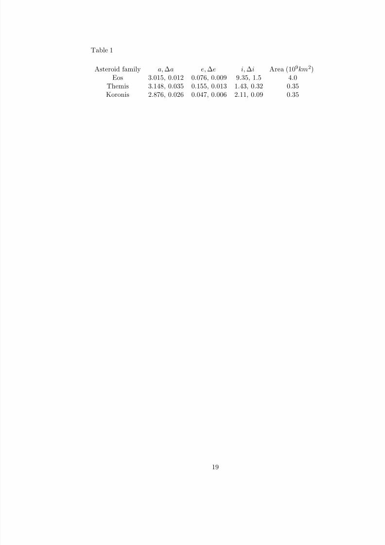
Table 1
Asteroid family a, ∆a e, ∆e i, ∆i Area (109km2)Eos 3.015, 0.012 0.076, 0.009 9.35, 1.5 4.0
Themis 3.148, 0.035 0.155, 0.013 1.43, 0.32 0.35
Koronis 2.876, 0.026 0.047, 0.006 2.11, 0.09 0.35
19
8/14/2019 The Size-Frequency Distribution of the Zodiacal Cloud- Evidence from the Solar System Dust Bands
http://slidepdf.com/reader/full/the-size-frequency-distribution-of-the-zodiacal-cloud-evidence-from-the-solar 20/46
Figure 1: IRAS observation of the zodiacal cloud in the 25 µm waveband (solid curve). Thisobservation was made at 90 solar elongation angle in the direction leading the Earth in itsorbit when the planet was at an ecliptic longitude of 293. The dust bands can be seen asprojecting ”shoulders” near ±10 and 0 latitude. The structure around 60 latitude is dueto dust in the plane of the Galaxy. By applying a Fourier filter to the IRAS observationa smooth background profile (underlying dotted curve) is separated from a high frequency
dust band profile (solid lower curve). This filtered high frequency dust band profile ismerely a residual representing the ”tip of the iceberg” in terms of dust band material inthe zodiacal cloud.
20
8/14/2019 The Size-Frequency Distribution of the Zodiacal Cloud- Evidence from the Solar System Dust Bands
http://slidepdf.com/reader/full/the-size-frequency-distribution-of-the-zodiacal-cloud-evidence-from-the-solar 21/46
Figure 2: The coefficient c represents the fraction of frequency points to remain after thehigh frequencies are stripped from the Fourier transform. This figure shows how moreand more of the original profile is incorporated into the low frequency background as theconstant c increases. This is a dramatic illustration of the arbitrary nature of any filtering
process and the danger of assuming the resultant residuals to represent the complete dustband structure.
21
8/14/2019 The Size-Frequency Distribution of the Zodiacal Cloud- Evidence from the Solar System Dust Bands
http://slidepdf.com/reader/full/the-size-frequency-distribution-of-the-zodiacal-cloud-evidence-from-the-solar 22/46
Figure 3: The variation with solar elongation angle of the latitude of peak flux of the northand south ten degree bands, at a longitude of Earth of 227.3 in the trailing direction.As the solar elongation angle increases, the effective distance to the dust band materialdecreases, and parallax causes the observed peak latitudes to increase. Over a small range
of solar elongation angle such as that shown, this effect can be assumed to be linear.
22
8/14/2019 The Size-Frequency Distribution of the Zodiacal Cloud- Evidence from the Solar System Dust Bands
http://slidepdf.com/reader/full/the-size-frequency-distribution-of-the-zodiacal-cloud-evidence-from-the-solar 23/46
Figure 4: The variation of the mean of the north and south ten degree band peak latitudesin the 25 µm waveband with ecliptic longitude of Earth. The sinusoidal variation indicatesthat the plane of symmetry of the bands is inclined to the ecliptic. The amplitude of thevariation is slightly more than one degree - close to the inclination of Jupiter’s orbit. Thisis an indication that the material associated with the bands is located in the asteroid belt.
23
8/14/2019 The Size-Frequency Distribution of the Zodiacal Cloud- Evidence from the Solar System Dust Bands
http://slidepdf.com/reader/full/the-size-frequency-distribution-of-the-zodiacal-cloud-evidence-from-the-solar 24/46
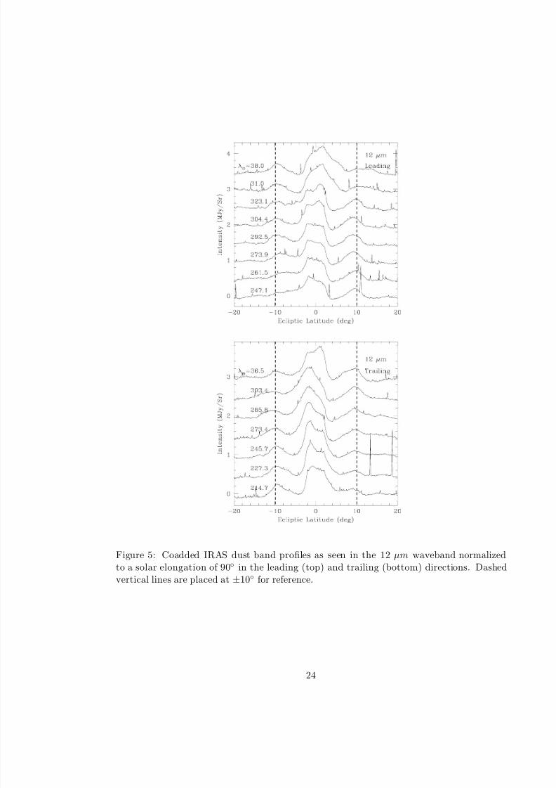
Figure 5: Coadded IRAS dust band profiles as seen in the 12 µm waveband normalizedto a solar elongation of 90 in the leading (top) and trailing (bottom) directions. Dashedvertical lines are placed at ±10 for reference.
24
8/14/2019 The Size-Frequency Distribution of the Zodiacal Cloud- Evidence from the Solar System Dust Bands
http://slidepdf.com/reader/full/the-size-frequency-distribution-of-the-zodiacal-cloud-evidence-from-the-solar 25/46
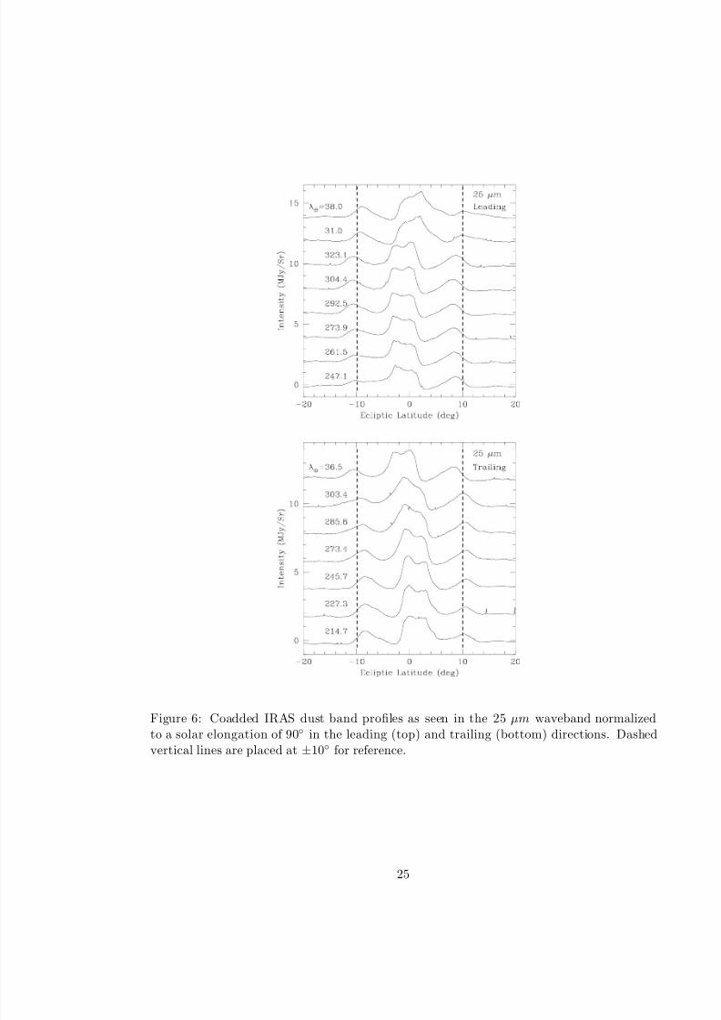
Figure 6: Coadded IRAS dust band profiles as seen in the 25 µm waveband normalizedto a solar elongation of 90 in the leading (top) and trailing (bottom) directions. Dashedvertical lines are placed at ±10 for reference.
25

8/14/2019 The Size-Frequency Distribution of the Zodiacal Cloud- Evidence from the Solar System Dust Bands
http://slidepdf.com/reader/full/the-size-frequency-distribution-of-the-zodiacal-cloud-evidence-from-the-solar 26/46
Figure 7: Coadded IRAS dust band profiles as seen in the 60 µm waveband normalizedto a solar elongation of 90 in the leading (top) and trailing (bottom) directions. Dashedvertical lines are placed at ±10 for reference.
26
8/14/2019 The Size-Frequency Distribution of the Zodiacal Cloud- Evidence from the Solar System Dust Bands
http://slidepdf.com/reader/full/the-size-frequency-distribution-of-the-zodiacal-cloud-evidence-from-the-solar 27/46
I sin Ω
I cos Ω
I
ΩΩ f
I f
Ωp
Ip
Figure 8: The vectorial relationship between the osculating, proper and forced elements in(I cos Ω, I sin Ω) space. The distributions are displaced from the origin due to the forcedelements and the radius of the distributions represents the proper elements. An equivalentrelationship exists for eccentricity and pericenter.
27
8/14/2019 The Size-Frequency Distribution of the Zodiacal Cloud- Evidence from the Solar System Dust Bands
http://slidepdf.com/reader/full/the-size-frequency-distribution-of-the-zodiacal-cloud-evidence-from-the-solar 28/46
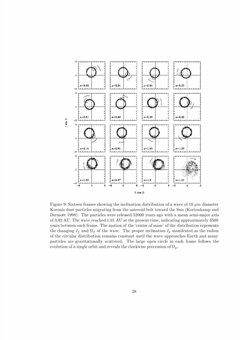
Figure 9: Sixteen frames showing the inclination distribution of a wave of 10 µm diameterKoronis dust particles migrating from the asteroid belt toward the Sun (Kortenkamp andDermott 1998). The particles were released 52000 years ago with a mean semi-major axisof 3.02 AU. The wave reached 1.01 AU at the present time, indicating approximately 3500years between each frame. The motion of the ‘center of mass’ of the distribution representsthe changing I f and Ωf of the wave. The proper inclination I p manifested as the radius
of the circular distribution remains constant until the wave approaches Earth and manyparticles are gravitationally scattered. The large open circle in each frame follows theevolution of a single orbit and reveals the clockwise precession of Ω p.
28
8/14/2019 The Size-Frequency Distribution of the Zodiacal Cloud- Evidence from the Solar System Dust Bands
http://slidepdf.com/reader/full/the-size-frequency-distribution-of-the-zodiacal-cloud-evidence-from-the-solar 29/46
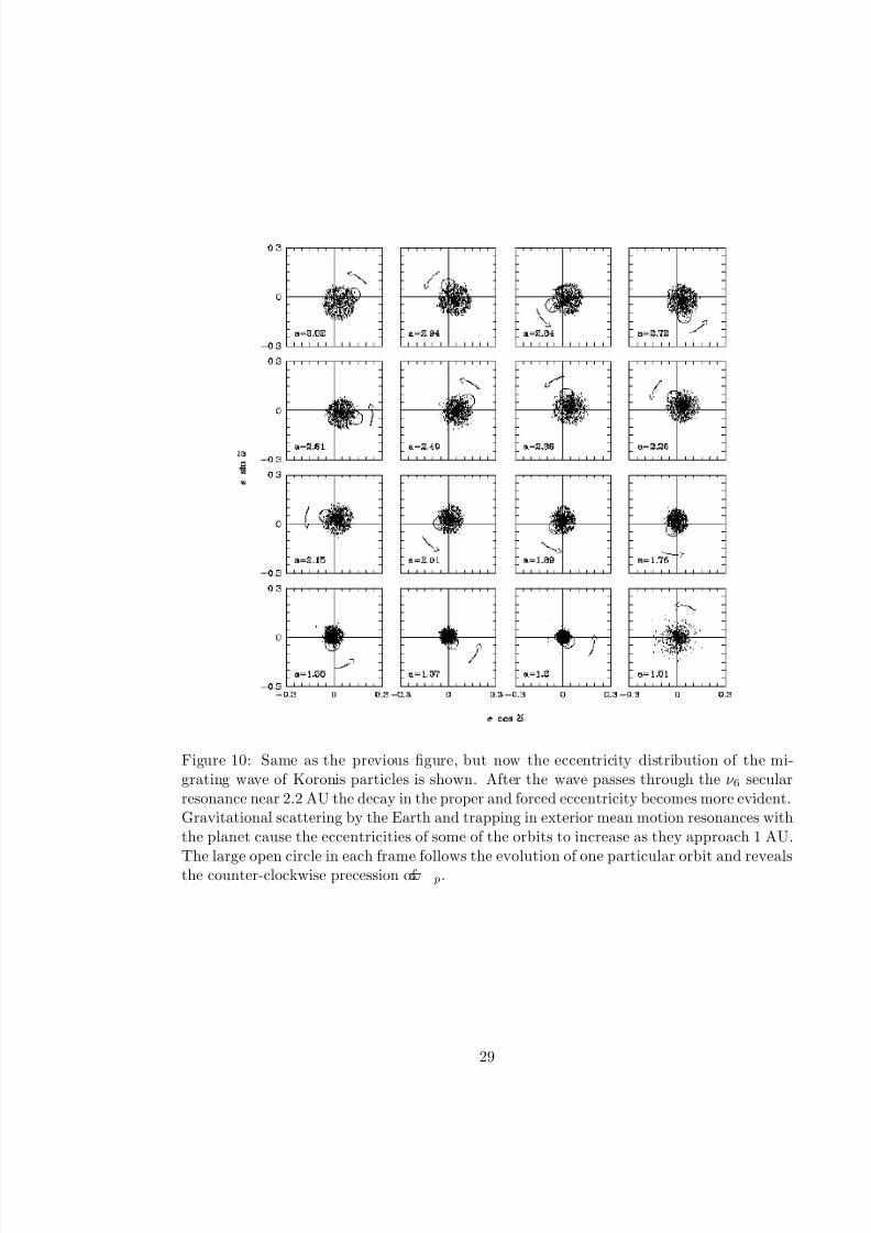
Figure 10: Same as the previous figure, but now the eccentricity distribution of the mi-grating wave of Koronis particles is shown. After the wave passes through the ν 6 secularresonance near 2.2 AU the decay in the proper and forced eccentricity becomes more evident.Gravitational scattering by the Earth and trapping in exterior mean motion resonances withthe planet cause the eccentricities of some of the orbits to increase as they approach 1 AU.
The large open circle in each frame follows the evolution of one particular orbit and revealsthe counter-clockwise precession of p.
29
8/14/2019 The Size-Frequency Distribution of the Zodiacal Cloud- Evidence from the Solar System Dust Bands
http://slidepdf.com/reader/full/the-size-frequency-distribution-of-the-zodiacal-cloud-evidence-from-the-solar 30/46
Figure 11: The iterative filtering procedure. Panel (a) shows a raw model dust band havingthe same viewing geometry as an observed background (b). In the first iteration (a) isadded to (b) and the sum is filtered to obtain (c), a model dust band (smooth curve); theobserved dust bands (noisy curve) are also shown for comparison. The background obtainedfrom this iteration shown in panel (d) is of a higher intensity than the original backgrounddue to the fact that it contains two low frequency dust band components, one from theaddition of the model dust band and one from the actual dust band in the original observedbackground. In the final iteration we subtract the excess intensity shown in (d) from theoriginal background (b) and add (a) before filtering to obtain the final dust band (e) andthe final background (f) that agree with the observations.
30
8/14/2019 The Size-Frequency Distribution of the Zodiacal Cloud- Evidence from the Solar System Dust Bands
http://slidepdf.com/reader/full/the-size-frequency-distribution-of-the-zodiacal-cloud-evidence-from-the-solar 31/46
Figure 12: The variation with heliocentric distance of the forced inclination (top) and node
(bottom) of dust particles in the zodiacal cloud. This variation is shown for five differentparticle sizes. The secular resonance near 2 AU has a dramatic effect which increases withparticle size: larger particles, having longer P-R drag lifetimes, spend a longer amount of time in the resonance.
31
8/14/2019 The Size-Frequency Distribution of the Zodiacal Cloud- Evidence from the Solar System Dust Bands
http://slidepdf.com/reader/full/the-size-frequency-distribution-of-the-zodiacal-cloud-evidence-from-the-solar 32/46
Figure 13: The variation with heliocentric distance of the forced eccentricity (top) and
pericenter (bottom) of dust particles in the zodiacal cloud. This variation is shown forfive different particle sizes. The secular resonance near 2 AU has a dramatic effect whichincreases with particle size: larger particles, having longer P-R drag lifetimes, spend a longeramount of time in the resonance.
32
8/14/2019 The Size-Frequency Distribution of the Zodiacal Cloud- Evidence from the Solar System Dust Bands
http://slidepdf.com/reader/full/the-size-frequency-distribution-of-the-zodiacal-cloud-evidence-from-the-solar 33/46
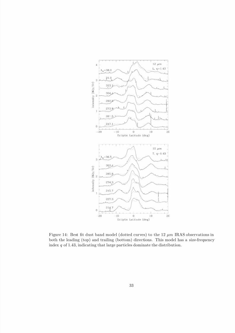
Figure 14: Best fit dust band model (dotted curves) to the 12 µm IRAS observations inboth the leading (top) and trailing (bottom) directions. This model has a size-frequencyindex q of 1.43, indicating that large particles dominate the distribution.
33
8/14/2019 The Size-Frequency Distribution of the Zodiacal Cloud- Evidence from the Solar System Dust Bands
http://slidepdf.com/reader/full/the-size-frequency-distribution-of-the-zodiacal-cloud-evidence-from-the-solar 34/46
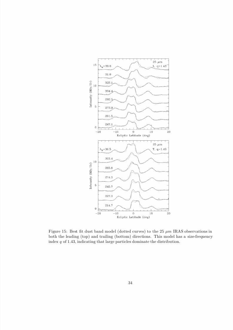
Figure 15: Best fit dust band model (dotted curves) to the 25 µm IRAS observations inboth the leading (top) and trailing (bottom) directions. This model has a size-frequencyindex q of 1.43, indicating that large particles dominate the distribution.
34
8/14/2019 The Size-Frequency Distribution of the Zodiacal Cloud- Evidence from the Solar System Dust Bands
http://slidepdf.com/reader/full/the-size-frequency-distribution-of-the-zodiacal-cloud-evidence-from-the-solar 35/46
Figure 16: Best fit dust band model (dotted curves) to the 60 µm IRAS observations inboth the leading (top) and trailing (bottom) directions. This model has a size-frequencyindex q of 1.43, indicating that large particles dominate the distribution.
35
8/14/2019 The Size-Frequency Distribution of the Zodiacal Cloud- Evidence from the Solar System Dust Bands
http://slidepdf.com/reader/full/the-size-frequency-distribution-of-the-zodiacal-cloud-evidence-from-the-solar 36/46
Figure 17: Goodness of fit of our models as a function of size-frequency index q for a singlelongitude of Earth. This has been obtained for the ten degree band by calculating theroot mean square (observation - model) over two five degree wide latitude bins to cover thenorth and south bands for both the 12 and 60 micron wavebands. When q is too high, toomany small particles are included in the model, and the amplitudes of the 12 µm modelsare too large. In addition, too few large particles are included and the amplitudes of the 60µm models are too small. When q is too low, too many large particles are included in the
model. This leads to the distribution of forced inclinations in the model to be skewed toomuch towards the large end, and the model profiles are shifted in latitude with respect tothe observations, degrading the fit. The particles are taken to be composed of astronomicalsilicate.
36

8/14/2019 The Size-Frequency Distribution of the Zodiacal Cloud- Evidence from the Solar System Dust Bands
http://slidepdf.com/reader/full/the-size-frequency-distribution-of-the-zodiacal-cloud-evidence-from-the-solar 37/46
Figure 18: Comparison of a q=1.83 dust band model (dotted curves) to the 12 µm IRASobservations in both the leading (top) and trailing (bottom) directions. Too many smallparticles are included in the model, and the ampitudes of the 12 µm models are too large.
37
8/14/2019 The Size-Frequency Distribution of the Zodiacal Cloud- Evidence from the Solar System Dust Bands
http://slidepdf.com/reader/full/the-size-frequency-distribution-of-the-zodiacal-cloud-evidence-from-the-solar 38/46
Figure 19: Comparison of a q=1.83 dust band model (dotted curves) to the 60 µm IRASobservations in b oth the leading (top) and trailing (bottom) (directions). Not enough largeparticles are included and the amplitudes of the 60 µm models are too small.
38

8/14/2019 The Size-Frequency Distribution of the Zodiacal Cloud- Evidence from the Solar System Dust Bands
http://slidepdf.com/reader/full/the-size-frequency-distribution-of-the-zodiacal-cloud-evidence-from-the-solar 39/46
Figure 20: The terrestrial influx of zodiacal dust particles, as measured from the crateringrecord on the LDEF satellite. The slope of area against particle mass indicates a value forq, the size-frequency distribution index, of approximately 1.15.
39

8/14/2019 The Size-Frequency Distribution of the Zodiacal Cloud- Evidence from the Solar System Dust Bands
http://slidepdf.com/reader/full/the-size-frequency-distribution-of-the-zodiacal-cloud-evidence-from-the-solar 40/46
Figure 21: Variation with wavelength and particle diameter of the absorption efficiencies of
astronomical silicate (top) and organic refractory material (bottom), calculated using Mietheory.
40
8/14/2019 The Size-Frequency Distribution of the Zodiacal Cloud- Evidence from the Solar System Dust Bands
http://slidepdf.com/reader/full/the-size-frequency-distribution-of-the-zodiacal-cloud-evidence-from-the-solar 41/46
Figure 22: The results shown in Figure 15 are repeated for organic refractory particles, toinvestigate the dependence of the modeling on the dust particle properties. The 12 micronresiduals strongly reinforce the result obtained with astronomical silicate that a low size-frequency index q is required to match the observations. The low emissivity of organicrefactories at longer wavelengths means that the 60 micron residuals are of little help in
pinning down the size-frequency distribution index, but even here the residuals decrease asq decreases.
41
8/14/2019 The Size-Frequency Distribution of the Zodiacal Cloud- Evidence from the Solar System Dust Bands
http://slidepdf.com/reader/full/the-size-frequency-distribution-of-the-zodiacal-cloud-evidence-from-the-solar 42/46
Figure 23: Eos family members, as determined by the hierarchical clustering method. Closedcircles represent asteroids larger than 15km in diameter, assuming an albedo of 0.12. Themean inclination of the model ten degree dust band material (9.35) is labeled. This suggeststhat either the ten degree band is produced from collisional activity near the inner edge of the family or that the inclinations of dust particle orbits from the Eos family as a whole
no longer trace the inclinations of their parent bodies but have been degraded since theirproduction.
42
8/14/2019 The Size-Frequency Distribution of the Zodiacal Cloud- Evidence from the Solar System Dust Bands
http://slidepdf.com/reader/full/the-size-frequency-distribution-of-the-zodiacal-cloud-evidence-from-the-solar 43/46
8/14/2019 The Size-Frequency Distribution of the Zodiacal Cloud- Evidence from the Solar System Dust Bands
http://slidepdf.com/reader/full/the-size-frequency-distribution-of-the-zodiacal-cloud-evidence-from-the-solar 44/46
Figure 25: The contribution of dust band material to the zodiacal cloud. The figure showsa comparison of the thermal emission obtained from the raw best fit dust band model tothe corresponding IRAS profile in the 25 µm waveband. The result is shown for innerSolar System distributions of material corresponding to γ =1.0, as expected for a systemevolved by P-R drag, and γ =1.3 as predicted in parametric models of the zodiacal cloud,most recently Kelsall et al. (1998). The dust bands appear to contribute approximately30% to the total thermal emission. Also shown is the amplitude of the dust band material
confined to the main belt (exterior to 2 AU), which represents the component of the dustband material isolated by the fast Fourier filter. This clearly shows the extent to whichthe dust band contribution is underestimated if it is assumed that the filtered dust bandobservations represent the entireity of the dust band component of the cloud.
44
8/14/2019 The Size-Frequency Distribution of the Zodiacal Cloud- Evidence from the Solar System Dust Bands
http://slidepdf.com/reader/full/the-size-frequency-distribution-of-the-zodiacal-cloud-evidence-from-the-solar 45/46
Figure 26: The ratio of areas of dust associated with the entire main belt asteroid populationand all families, obtained by extrapolating the observed size distributions of larger asteroidsin both populations assuming a collisional equilibrium power law size distribution.
45
8/14/2019 The Size-Frequency Distribution of the Zodiacal Cloud- Evidence from the Solar System Dust Bands
http://slidepdf.com/reader/full/the-size-frequency-distribution-of-the-zodiacal-cloud-evidence-from-the-solar 46/46