THE SIMPLEX-SIMULATED ANNEALING APPROACH...

Computers chem. Engng Vol. 2(I, No. 9, pp. 1065-1080, 1996 Pergamon Copyright (~) 1996 Elsevier Science Ltd

Printed in Great Britain. All rights reserved 0098-1354(95)00221-9 1X198-1354/96 $15.00 + 11.111

THE SIMPLEX-SIMULATED ANNEALING APPROACH TO CONTINUOUS NON-LINEAR OPTIMIZATION

MARGARIDA F. CARDOSO, R. L. SALCEDOt and S. F E v o DE AZEVEOO

Departamento de Engenharia Quimica, Faculdade de Engenharia da Universidade do Porto, Rua dos Bragas, 4099 Porto, Portugal

(Receiued 30 November 1994; final revision received 5 April 19951

Abstract--An algorithm suitable for the global optimization of nonconvex continuous unconstrained and constrained functions is presented. The scheme is based on a proposal by Press and Teukolsky (Comput. Phys. 5(4), 426, 1991) that combines the non-linear simplex and simulated annealing algorithms. A non-equilibrium variant will also be presented, whereby the cooling schedule is enforced as soon as an improved solution is obtained. The latter is shown to provide faster execution times without compromising the quality of the attained solutions.

Both the algorithm and its non-equilibrium variant were tested with several severe functions published in the literature. Results for nine of these functions are compared with those obtained employing a robust adaptive random search method and the Nelder and Mead simplex method (Comput. J. 7,308, 1965). The proposed approach is shown to be more robust and more efficient in what concerns the overcoming of difficulties associated with local optima, the starting solution vector and the dependency upon the random number sequence. The results obtained reveal the adequacy of the algorithm for the global optimization of a broad range of problems encountered in chemical engineering practice. Copyright © 1996 Elsevier Science Ltd

I. INTRODUCTION accuracy within a finite number of iterations. With nonconvex functions and constraints, the presence

The optimization of non-linear constrained prob- of local optima is difficult to deal with, since most lems is relevant to chemical engineering practice, optimization algorithms are of the "local search" Non-linearitiesare introduced by processequipment type and will eventually get trapped in a local design relations, by equilibrium relations and by optimum. This is particularly true for derivative combined heat and mass balances, and constraints algorithms, but still highly relevant for direct are due to limits imposed on design variables and on (derivative-free) methods. It should be noted that inequality relations between dependent and inde- currently available algorithms for nonconvex NLP pendent variables. The design variables may be problems can lead to sub-optimal solutions as noncontinuous [non-linear programing (NLP) prob- convexities may cut off the global optimum from the lems] or some may be integer [mixed-integer non- current search regions (Wang and Luus, 1978; Kocis linear programming (MINLP) problems]. For the and Grossmann, 1988; Floudas et al., 1989). case of NLP problems, the general statement is: Adaptive random search methods are particularly

attractive for the global optimization of nonconvex minimize F(0) (1)

problems and are easily applicable to constrained subject to the inequality constraints: functions. Some examples include the Luus and

Jaakola algorithm (Luus and Jaakola, 1973) and gi(0)~>0 j = 1 , 2 . . . . . M (2) improved variants (Gaines and Gaddy, 1976;

and to the bound constraints: Heuckroth et al., 1976; Wang and Luus, 1977; Martin and Gaddy, 1982; Salcedo et al., 1990),

ai~Oi~fli i = 1 , 2 . . . . . N (3) modified Matyas algorithms (Mihail and Maria,

where 0 represents the vector of optimization para- 1986; Maria, 1989) and search clustering algorithms meters and (ai, f l i) are bounds on parameter 0,. (Price, 1978; TOrn, 1978). Although beyond the

The efficiency of optimization routines is linked to scope of this paper, a further advantage of adaptive their ability in reaching the optimum with a desired random search methods is in their ability to handle

MINLP problems directly, at least of moderate

t Author to whom all correspondence should be dimension (Campbell and Gaddy, 1976; Salcedo, addressed. 1992).

1065

1066 M.F. CARDOSO et al.

The ability of random search methods to escape equilibrium simulated annealing scheme (Cardoso et

difficult local optima can be attributed to the al. , 1994) leads to a variant (the NE-SIMPSA algor- random nature of the search space. Such desirable ithm) which decreases the computational burden feature is significantly enhanced when the random without significantly compromising the quality of the method incorporates shifting strategies allowing for attained solutions. "wrong-way" moves to be produced. These strate- Comparison is made with a robust adaptive gies may be simple heuristics that penalize the cur- random search method available (Salcedo et al. ,

rent solution vector, guiding the algorithm towards 1990; Salcedo, 1992) and with the Nelder and Mead diverse regions within the search space (Satcedo et (1965) simplex algorithm. The approach proposed in al. , 1990) or more sophisticated penalizing func- this paper shows a superior performance in over- tions, coming local optima and accuracy. All nine test

Simulated annealing is a powerful technique for functions employed for the analysis of performance combinatorial optimization, i.e. for the optimization were proposed by independent authors and cover a of functions that may assume several distinct dis- broad range of difficult optimization problems. crete configurations (Metropolis et al. , 1953; Thus, the SIMPSA and the NE-SIMPSA algorithms Kirkpatrick et al . , 1983; Kirkpatrick, 1984). represent interesting alternatives for the global opti- Algorithms based on simulated annealing employ a mization of NLP problems typical of chemical engi- stochastic generation of solution vectors and employ neering practice. similarities between the physical process of anneal-

ing (i.e. melting a solid by heating it, followed by SIMULATED ANNEALNG FOR COMBINATORIAL slow cooling and crystallization into a minimum free

MINIMIZATION energy state) and a minimization problem. During the cooling process, transitions are accepted to Annealing is the physical thermal process of melt- occur from a low to a high energy level through a ing a solid by heating it, followed by slow cooling Boltzmann probability distribution. For an optimi- and crystallization into a minimum free energy state. zation problem, this corresponds to "wrong-way" If the cooling rate is not carefully controlled or the movements as referred to above, initial temperature is not sufficiently high, the cool-

Other direct methods, albeit deterministic, also ing "solid" does not attain thermal equilibrium at possess some ability to escape local optima. One of each temperature. In such circumstances, local opti- the most robust with respect to this feature, for mal lattice structures may occur, which translate unconstrained problems, is the non-linear simplex into lattice imperfections. Thermal equilibrium at a method of Nelder and Mead (1965). This is a direct given temperature is characterized by a Boltzmann algorithm that does not require derivative (either distribution function of the energy states. Under first or second order) information. The simplex these conditions, even at a low temperature, albeit method has been exhaustively studied by many with a small probability, a transition may occur from researchers, among them Olson and Nelson (1975) a low to a high energy level. Such transitions are and Barabino et al. (1980). Basically (Nelder and assumed to be responsible for the system reaching a Mead, 1965; Tao, 1988; Edgar and Himmeiblau, minimum energy state. 1988), the methods proceeds by generating a sim- The Metropolis algorithm (Metropolis et al. ,

plex (with N dimensions, a simplex is a hypergeo- 1953; Kirkpatrick et al. , 1983; Kirkpatrick, 1984) metric figure generated by joining N + I points in was the first proposed to simulate this process. the N-dimensional space) which evolves at each Starting from a high energy state, corresponding to a iteration through reflexions, expansions and con- particular system temperature T j, a series of new tractions in one direction or in all directions, so as energy states E j are stochastically generated. Each mostly to move away from the worst point, new system configuration is accepted if E j+ i ~< E j.

In this work, we present an algorithm based on Otherwise, and by analogy with the Boltzmann the combination of the non-linear smplex and simu- distribution for energy states at thermal equilibrium, lated annealing algorithms (the SIMPSA algorithm) E j will be accepted as an improved state with a which is shown to be adequate for the global optimi- probability determined by P ( A E ) = zation of an example set of unconstrained and con- e x p ( - ( E j+ ~ - E i ) / ( K ~ TJ)), where T j is the current strained NLP functions. The algorithm relies on a system temperature and KB is Boltzmann's constant. scheme proposed by Press and Teukolsky (1991) At high temperatures this probability is close to one, incorporating important additional features, such as viz . most energy transitions are permissible. As the the ability to handle constraints and appropriate system temperature decreases the probability of termination criteria. The adoption of a non- accepting a higher energy state as beingan improved

Simplex-simulated annealing algorithms 1067

energy state approaches zero, and it is assumed that to be the major stumbling block for the effective thermal equilibrium is reached at each temperature, application of simulated annealing to the optimiza-

From an optimization point of view, simulated tion of continuous spaces (Vanderbilt and Louie, annealing explores the key feature of the physical 1984; Press and Teukolsky, 1991). annealing process of generating transitions to higher Corana et al. (1987) derived a global continuous energy states, applying to the new states an optimizer based on simulated annealing, by coupling acceptance/rejection probability criterion which the acceptance/rejection criteria of the Metropolis should naturally become more and more stringent algorithm with a random search that progresses with the progress of the procedure. For solving a along each coordinate axis. The algorithm was particular problem with a simulated annealing algor- tested against both the Nelder and Mead (1965) ithm, the following steps are thus necessary: simplex method and an adaptive random search

method (Masri et al., 1980; Pronzato et al., 1984); (i) Definition of an objective function to be

minimized, for difficult unconstrained functions, up to 10 dimensions, it was found to be more robust in

(ii) Adoption of an annealing cooling schedule, overcoming local optima, albeit at a great expense in

whereby the initial temperature, the number of configurations generated at each temperature and computational burden. This algorithm may, how-

ever, produce poor results for the optimization of a method to decrease it are specified.

cost functions having "valleys" not directed along (iii) At each temperature in the cooling sche-

the coordinate axis (Corana et al., 1987). It is note- dule, stochastic generation of the alternative combinations, centered on the currently accepted worthy to mention that, apart from the occurrence

of a few local optima, the simplex method required state, much fewer function evaluations to locate the global

(iv) Adoption of criteria for the acceptance or optima than both the simulated annealing and the

rejection of the alternative combinations, against adaptive random search algorithms (by about a

the currently accepted state at that temperature. factor of 500-1000). Groisman and Parker (1993)

The vast majority of applications of simulated have applied the Corana et al. (1987) algorithm for annealing have been related to combinatorial mini- the solution of least-squares problems in applied mization problems, such as the classical traveling photometry. salesman problem (Press et al., 1986; Salcedo et al., Bohachevsky et al. (1986) used a slightly different 1993; Cardoso et al., 1994), heat-exchanger and scheme, whereby the random directions of simu- pressure-relief header networks (Dolan et al., 1989, lated annealing were computed from independent 1990; Cardoso et al., 1994), complex rectification standard normal variates and the random steps were column sequencing (Floquet et al., 1994), graph problem dependent. They have applied their algor- partitioning (Johnson et al., 1989), optimization of ithm to the solution of simple multimodal 2-D physical data tables (Corey and Young, 1989), batch unconstrained functions and to a more complex process scheduling (Das et al., 1990; Ku and Karimi, constrained design problem in neuroscience involv- 1991; Patel et al., 1991), graph colouring and ing 11 degrees of freedom. n u m b e r p a r t i t i o n i n g ( J o h n s o n e t a l . , 1991) and imag- Vanderbilt and Louie (1984) proposed a self- ing applications (Silverman and Addler, 1992; regulatory search mechanism for the continuous Groisman and Parker, 1993). An overview of simu- vector 0, which guarantees that the annealing pro- lated annealing as applied to combinatorial minimi- ceeds in an efficient and anisotropic way, i.e. main- zation can be found in Aarst and Korst (1989) and in taining a biased random walk towards the global Ingber (1993). minimum. They have applied their algorithm to

difficult unconstrained mathematical functions and SIMULATED ANNEALING FOR CONTINUOUS found it to be competitive with adaptive random

OPTIMIZATION search and search cluster methods (Price, 1978;

Simulated annealing has also been applied to the T6rn, 1978). Vanderbilt and Louie (1984) further optimization of multimodal continuous spaces (Van- suggest that their approach could be integrated with derbilt and Louie, 1984; Bohachevsky et al., 1986; search clustering or with the simplex method, to Corana et al., 1987; Press and Teukolsky, 1991) and improve performance. this is the subject of the present work. For such Press and Teukolsky (1991) have reviewed the problems, the system state (or configuration) is basic approaches behind the application of simu- simply the continuous vector 0 and one must lated annealing to continuous optimization, and provide some means of generating alternative confi- have proposed, in our opinion, a very interesting gurations starting from the current one. This seems and potentially robust scheme - - combining the


stochastic simulated annealing algorithm with the schedule may be enforced as soon as an improved simplex method of Nelder and Mead (1965). solution is obtained. This modification corresponds However, these authors do not show any data to to a non-equilibrium situation and to a change in the substantiate the performance of the proposed algor- termination criterion for the inner loop. ithm. At the start of the optimization, the solution is

most probably far from the optimum and CPU time

THE SIMPSA AND NE--SIMPSA ALGORITHMS is not wasted in the search for a near-equilibrium state. As the optimization proceeds, the "tempera-

In this work, the original Metropolis algorithm ture" control parameter drops and solution accep- and its non-equilibrium variant (NESA/Metropolis; tance is decided according to the Metropolis algor- Cardoso et al., 1994) were combined with the sim- ithm. It will eventually drop to a point where no plex algorithm as proposed by Press and Teukolsky more poorer acceptances are allowed, thus assuring (1991), giving rise to the SIMPSA and NE-SIMPSA convergence to a local optimum, as in the patterns algorithms, observed for the original simulated annealing pro-

The role of simulated annealing in the overall cedures. This non-equilibrium scheme has been approach is to allow for wrong-way movements, tested with combinatorial minimization and shown simultaneously providing (asymptotic) convergence to produce significantly faster convergence to the to the global optimum. The main aspects are the global optimum (Salcedo et al., 1993; Cardoso et al., acceptance/rejection criteria, the initial annealing 1994). In the present paper, we show that the non- temperature and the adoption of a suitable cooling equilibrium variants of simulated annealing also give schedule. The role of the non-linear simplex is to good results for non-linear continuous optimization, generate system configurations. The main differ- in a fraction of the time needed by the equilibrium ences between the proposed algorithms and that of Metropolis algorithm. Press and Teukoisky are:

Initial annealing temperature - - t h e ability to deal with constraints The initial control temperature is an important - - the adoption of a cooling schedule based on the parameter which can be obtained by specifying the

global centroid fraction of generated solutions to be accepted - - t h e adoption of a contraction scheme for the initially (Aarst and Korst, 1989; Ku and Karimi,

parameter search space, commanded by the 1991; Patel et al., 1991). It is important that the cooling schedule, whereby toggling is made initial temperature control parameter be estimated between the global and the contracted search such that the acceptance probabilities are close to

space one. For this purpose, in this work, the initial - - t h e inclusion of an additional stopping criter- temperature Ti was estimated by:

ium which produces a faster non-equilibrium variant of simulated annealing. m, + m~ exp ( - Af+']

- \ T, ] All of these aspects of the algorithms are described X - (5) next. m~ + m2

The equilibrium and non-equilibrium Metropolis where the acceptance ratio X was set to 95% (Aarst algorithms and Korst, 1989). For a universe of m0 combi-

With the Metropolis algorithm, the probability of nations, and in a sequential analysis, m~ represents the number of successful moves (E k < E k- ~ for k = 2

acceptance of new configurations (solutions) is as follows: to m0), m 2 the number of unsuccessful moves

(Ek~ > E k-j) and Af + the average increase in cost for P = 1 AC < 0 the m2 unsuccessful moves.

As with combinatorial optimization, m0 was set to = exp( - AC/KR T) AC>I 0 (4) 100 × N, where N represents the number of dimen-

where AC is the difference in cost between a newer sions (Cardoso et al., 1994). To apply equation (5) configuration and the current solution, Ko is to the continuous case, a preliminary high tempera- Boltzmann's constant and Tis the annealing temper- ture was estimated by multiplying the absolute value ature. The Metropolis algorithm enforces the cool- of the objective function corresponding to the starting schedule only after a large number of trials have ing solution vector by a large positive value (e.g. been evaluated, in order to reach equilibrium at 105). This high temperature allows all moves to be every temperature level. To reduce the computatio- initially accepted, and after m0 moves corresponding nal burden associated with this scheme, the cooling to a full Metropolis cycle are completed, the initial


temperature Tiin equation (5) is computed from the above[ for the evaluation of the initial annealing values of mr, m2 and Af +. The cooling schedule will temperature. With the non-equilibrium variants, the then proceed with this temperature value, temperature also decreases as soon as an improved

Cooling schedule solution is obtained. Since a representative point on which to measure this improvement is needed, the

The cooling schedule employed was the Aarst and global centroid (incorporating all current simplex

van Laarhoven (1985) scheme: vertices without considering constraints) was

T j employed. The main idea is that the global centroid TJ+~- Ti.ln(1 +6 ) (6) is the most appropriate indicator of the simplex

1+ 30 movement. Tests performed showed that better results were obtained using the global centroid

where 6 and a are trajectory parameters and j is the rather than using the centroid with the exclusion of current iteration. The parameter 6 controls the cool- the worst point, as is usually done in the simplex ing rate and is a measure of the desired closeness to method. This global centroid was also used by equilibrium (Das et al., 1990; Patel et al., 1991). Adelman and Stevens (1972) in their implemen- Small values ( < 1) produce slow convergence and tation of a constrained version of the simplex large values ( > 1 ) produce convergence to poor method, viz. a variant of the Complex method of local optima. The parameter a is the standard devi- Box (1965). ation of all cost configurations at the current temperature T j. Generating the initial simplex

Alternative cooling schedules are usually of the exponential type (Kirkpatrick et al., 1983), where a To solve an N-D problem, it is necessary to constant multiplicative factor is employed to obtain generate N + 1 points that form the vertices of the the new temperature. Tests performed with combi- N-D simplex. natorial minimization (Aarst and Korst, 1989; Das et For unconstrained problems, this was performed al., 1990; Dolan et al., 1990; Patel et al., 1991; by the following rule: Cardoso et al., 1994) lead to verify that simulated

0i = 00 + (0.5-rnd) x 2 x abs(00) (7) annealing performed better with the Aarst and van Laarhoven scheme [equation (6)], rather than with where 00 is any initial N-D point, rnd is a pseudo- the exponential decrease in temperature, random number between 0 and 1 and abs is the

At this point, it is important to distinguish non- absolute value of the N components of the initial equilibrium simulated annealing (NESA) from vector 00. However, other schemes are equally poss- simulated quenching (Ingber, 1993), which results ible. from the use of faster cooling schedules in order to For constrained problems, the initial simplex was reduce the computational burden. With non- generated by: equilibrium simulated annealing, slow cooling sche-

0/= 00 + (0.5-rnd) x K j x ( f l i - ai) (8) dules should be employed to provide smooth temperature trajectories similar to those found in the which is the continuous parameter generation original Metropolis scheme and minimize the scheme employed in the SGA/MSGA algorithms chances of convergence to local optima. The cooling (Salcedo et al., 1990; Salcedo, 1992). K j is a variable schedule and the acceptance criterion have a cou- factor, as shown below [equation (9)], and j is the pled effect on convergence. Consequently, the same current global iteration. value of 6 will produce significantly different trajec- It should be stressed that equation (8) does not tories for the nonequilibrium and equilibrium vari- guarantee feasibility, with respect either to the ants. With combinatorial minimization, it was found inequality [equation (2)] or to the bound [equation (Cardoso et al., 1994) that the 6 value for the non- (3)] constraints. It was found that the proposed equilibrium algorithm had to be about three orders algorithms sometimes collapsed on infeasible points of magnitude smaller than that corresponding to the if the initial solution vector 00 did not obey all bound equilibrium algorithm, in order to produce similar constraints. In this case, equation (8) might not be smooth cooling schedules. The same ratio was thus able to generate simplex vertices within the bound employed in the present work. constraints, evolving towards a region of total infea-

According to Press and Teukolsky (1991), the sibility from where the algorithms may not recover. temperature should be decreased after a fixed Thus, in the SIMPSA and NE-SIMPSA algorithms, number of iterations within the simplex method, equation (8) is repeatedly employed until all vertices Here, this number was set at 100×N, as stated obey all bound constraints (but not necessarily the


inequality constraints), starting from either a feas- applicable to constrained functions (the Complex ible or an infeasible point. In this work, for compari- method) based on the simplex method of Nelder and son purposes, we have employed the starting points Mead. Thus, it seemed logical to replace, within the proposed by independent authors. In a general proposed scheme, the simplex method with the application, a simple choice for a starting solution Complex method of Box (1965). Basically, Box vector which obeys all bound constraints is the proposed that if one bound constraint [equation (3)] middle of the search intervals. This has also been is violated, the variable takes the value of the tested, having led to similar results, constraint, and if an inequality (or implicit) con-

straint is violated [equation (2)], the new point Generation o f system configurations would move half-way from the distance that separ-

The generated configurations are options pre- ates it from the centroid of the remaining points sented to the system. For combinatorial minimiza- (Adelman and Stevens, 1972; Edgar and tion, the generation of each system configuration on Himmelblau, 1988).

an N-D space, specified by the vector components 0j We tested several problems with this approach, (j = 1, N), from the previous solution 9~ (i = 1, N), and in most cases degenerate simplexes would occur may be problem dependent. It may be obtained by collapsing on an infeasible centroid. This could in simple random changes (Dolan et al., 1989) or may principle be solved by restarting periodically the include some heuristic guidance (Press et al., 1986). algorithm or by using more complex vertex replace-

For the case of continuous optimization, the gene- ment schemes (Umeda and Ichikawa, 1971), but a ration of the system state is based on the simplex more convenient and simple method was sought - - method of Nelder and Mead (1965), whereby the this consists of substituting points produced by the design vector 0 is replaced by an N-D simplex. Press simplex movement that do not obey either bound or and Teukolsky (1991) add a positive logarithmic implicit constraints by randomly generated points distributed variable, proportional to the control centered on the current best vertex, through the use temperature T, to the function value associated with of equation (8), where O0 is now the best vertex. every vertex of the simplex. Likewise, they subtract Infeasible points may still be replaced by infeasible a similar random variable from the function value at points, except that they are now centered on the every new replacement point. These schemes are best vertex and obey all bound constraints. represented by the following relations: To ensure convergence of the evolving simplex,

(Fperturt, e0)k = F k - T x In(rnd); k = 1, N + 1 (9) the parameter K j in equation (8) was made variable with the global iteration j, following the Aarst and

(Fperturbed)new = Fo~w+ T× ln(rnd) (10) van Laarhoven (1985) scheme [equation (6)]. This

where F~ is the function value for vertex k, F,~w is shrinking effect on the size of the region centered on the function value at the replacement point and the current best vertex may, however, guide the Fperturbe d is the perturbed function value. For a mini- algorithm too fast towards a local optimum from mization problem, the N + 1 vertices are perturbed which it may not be able to escape. Thus, the towards higher function values, according to equa- compression factor K i is only activated once every tion (9), whereas the replacement point is perturbed two global iterations, oiz. the algorithm toggles towards a lower value, following equation (10). between a search with the global intervals and a Thus, if the replacement point corresponds to a search with compressed intervals, viz.:

lower cost, this method always accepts a true dewn- K i = 1 j odd hill step. If, on the other hand, the replacement

T ) point corresponds to a higher cost, an uphill move K/= K / 2 j even. (11) may be accepted, depending on the relative costs of T' the perturbed values. This is the principle behind the Metropolis algorithm, and has the advantage of All infeasible points are penalized by assuming a reducing to the simplex method as T---~0. This very large positive value for a minimization problem approach has been retained in the present work. or a very large negative value otherwise. It may

obviously occur that all points in the simplex end up Dealing with constraints penalized. However, quantitative comparison

This is an important and difficult question that between these points, which is needed both for the affects most optimization problems with interest to simplex algorithm and for the Metropolis algorithm, chemical engineering. However, this point is not is still possible, since a random perturbation pro- addressed by Press and Teukolsky (1991). Box portional to the temperature control parameter is (1965) has developed an optimization algorithm superimposed on the function values [equations (9)


and (10)]. The simplex will then proceed with reflec- the relative error in the objective function, averaged

tions, expansions or contractions through the cen- over a fixed number of function evaluations. Here, troid, defined here as usually, viz. incorporating all just as for the cooling schedule, the global centroid current vertices with the exception of the worst is employed to compute the cost term needed for the point, successive comparisons.

Thus, unlike direct random search methods such

as the MSGA algorithm, which are feasible path NUMERICAL IMPLEMENTATION AND CASE-STUDIES methods, the proposed algorithms are infeasible path methods, since they can proceed through corn- The SIMPSA and the NE-SIMPSA algorithms parisons of infeasible vertices. For highly nonconvex were written in FORTRAN 77 and all runs were problems, it may be very difficult to generate points performed with double precision on an HP730 on the surface described by inequality constraints, workstation, running compiler optimized With degenerate simplexes, the periodic setting of FORTRAN 77 code. To state the quality of the K j = 1 makes the overall search space available for proposed algorithms, comparison with another glo- the generation of new solutions. This avoids the bal optimizer is needed. The MSGA adaptive need of periodically restarting the algorithm, since random search algorithm (Salcedo et al., 1990; the probability of obtaining a feasible vertex Salcedo, 1992) was implemented in the same works- increases. On the other hand, when some vertex is tation and used for this purpose. feasible, the adoption of a shrinking search space Simulated annealing and random search methods increases the probability of finding a nearby feasible are stochastic, and as such can be sensitive to the point, thus guiding the algorithm towards feasibility, sequence of pseudo-random numbers. In this work,

As the objective functions of the proposed algor- a Lehmer linear congruential generator (Shedler, ithms do not include any information about the 1983) was used, which was tested for multidimensio- extent of constraint violations, there is no guarantee hal uniformity and found to be satisfactory (Salcedo

that a feasible point will be found. However, the et al., 1990). proposed algorithms were able to converge to feas- Performance evaluation was carried out by statis- ible points that correspond to several active inequa- tical evaluation of nine severe unconstrained and lity constraints, which is the case for the global constrained functions taken from the literature. The optima of all constrained problems tested in the constrained functions are all nonconvex (multimo- present work. dal), used by other authors to test robustness in

Termination criteria surpassing local optima. The unconstrained functions include difficult ill-conditioned least-squares

The proposed algorithm includes two conver- examples.

gence tests. One is inherent to the simplex method, The error criteria used in the present work were as implemented by Press et al. (1986) and Press and set at 10 8, both for the convergence of the simplex Teukolsky (1991) and is a measure of collapse of the algorithm as given by Press and Teukolsky (1991) centroid. The second criterium was employed and for the smoothed function values as given by before for combinatorial minimization and is based equation (12). For the unconstrained functions, the on an averaged gradient of the objective function cooling schedule b values were set at 10 and 10 -2, with respect to the number of function evaluations, respectively for the equilibrium (SIMPSA) and non- This has been shown to be an efficient criterion for equilibrium (NE-SIMPSA) algorithms. The

the non-equilibrium simulated annealing algorithms Rosenbrock function in four dimensions was tested (Cardoso et al., 1994). To implement such a criter- with another value for 6 to provide some indication ion while smoothing out fluctuations in the objective of the influence of this parameter. For the con- function, groups of 5 × N values were averaged. The strained functions, which are more difficult, lower normalized gradient was computed from these aver- values for 6 were employed, respectively 10 1/10-4.

ages, as follows: Whenever different values for 6 were used, in order

1 d C * C ~ - - C i*-i to improve results, this is explicitly referred to in the - < e (12) discussion.

C~ dN C * ( N i - N i - I ) All problems were run with 100 different seeds.

where 0 < e ' ~ l , Ni is the cumulative number of For the SIMPSA, NE-SIMPSA and unconstrained function evaluations at iteration i and C,* the and constrained simplex, this corresponds to the respective averaged cost. Since the factor Ni-PC,-_~ generation of 100 different initial simplexes. It also is constant (in our case equal to 5 x N), the gradient corresponds to stochastic movements, whenever given by equation (12) is simply an expression for bound constraints are violated, through the use of

1072 M . F . C A ~ t ) o s o et al.

Table 1. Test functions for optimization procedures

Case Type of Type of Number of number Authors problcm optimization parameters General comments

1 Rosenbrock (1960) MF UMIN 2/4 Stccp-sided parabolic vallcy 2 Colville (1968) MF UMIN 4 Difficult saddle point 3 Dixon (19731 MF UMIN 111 Difficult local optimum 4 Meyer and Roth (19721 MF ULS 3 Extrcmcly ill-conditioned 5 Nash and Walker-Smith (19871 MF ULS 6 Triplc exponential; difficult to fit 6 Luus (1974) MF C M A X 3 Four local maxima 7 Luus and Jaakola (1973) CEP CMIN 3 Difficult local minima 8 Luus (1975) CEP C M A X 5 Difficult local maxima 9 Grossmann and Sargent (1979) CEP CMIN 7 Optimization of multicrudc pipelinc

Type of Problem: MF = mathematical function; CEP = chemical cngineerng problem. Type of Optimization: C M A X = constrained maximization; CMIN - constrained minimization; UM1N = unconstrained minimization; ULS = unconstrained least-squares.

equation (8). Further, for the SIMPSA and constant at around 35000, irrespective of the prob- NE-SIMPSA algorithms, the different seeds also lem dimension or difficulty (Salcedo et al., 1990; provide different optimization paths since a random Salcedo, 1992). perturbation is superimposed on the simplex ver-

tices, as discussed before. For the MSGA algorithm, RESULTS AND DISCUSSION the different seeds simply provide different optimization paths as they directly affect the stochastic

Unconstrained minimization generation of solution vectors. Some problems were also run with different start- The problems represented by functions 1-5 of

ing points to provide a measure of the influence of Table 1 were chosen to illustrate the behavior of the the initial conditions. The initial search regions, for SIMPSA algorithms for unconstrained minimiza- constrained optimization, were determined from the tion. The corresponding functional expressions and bound constraints. Where appropriate, results are data are given in Table 2. Here, sets of 100 different also compared on the basis of accuracy in reaching a seeds were employed with each algorithm, for every value of the objective function within a percentage starting point. of the global optimum. The average number of The results are summarized in Table 3. For func- function evaluations as well as the average CPU tion 1, 2-D, all algorithms performed well, reaching times are also given. With the MSGA algorithm, the the global optimum of (1, 1) r. The average execu- number of function evaluations is approximately tion times were 0.35 s, 0.41s, 0.67 s and 0.81 s,

Table 2. Unconstrained function

Global optimum Function Test function Initial values (author)

la Rosenbrock (1960) y = 100(0{ - 02) 2 + (1 -- 01)2 0 = [ -- 1.2, lff 0 = [I , 1] / F = 24.2 F = 0

3

{1oo(o~-o,, i ) ' + ( l lb Rosenbrock (1960) Y=~.~ 0 = [ - 1.2, 1, - 1.2, 1] ~ 0 = [ 1 , 1, 1, 1] ~ '= ~ F = 532.4 F = 0

2 Colville (1968) y = 100 (0 ] - 0z)2 + (0~ - 1)2+ (0~- 1) 2 0 = [ - 3 , - I , - 3 , - 1 ] t O= [ l, l, l, l ff + 9(1(03- 04) 2 + 10.1((02- 1 )2 F = 19192 F = (I + (04- I) 2) + 19.8(0.~- 1)*(04- 1 )

3 Dixon(1973) Y = ( l - 0 0 : + ( 1 - 0 u ' ) 2 + E ( 0 ~ - 0 i + 0 2 i ~ , 0F-~42 . . . . . - 2 I t OF=[] . . . . . 1]'

4 Meyer and Roth (1972) y = a* exp[b/(c + x)] 0 = [(I.02, 4(1(X), 250] t 0 = 1(1.(X156, 6181.4,345.21 t F = 1.7 × 1(1 v F = 88

3

5 Nash and Walker-Smith (1987) y = ~ [0~i t cxp - (02 ,x ) ] 0 = [ 1 , 1 , 1,2, 1,3] r 0=[0 .0951 , 1, 0.8607, 3, i = l

1.5567, 5] t F = 12.1 F = I )

With the following values applicable: Function 4: x 50 55 60 65 70 75 80 85 90 95 IIX) 11)5 110 115 120 125

y 34780 28611) 23650 19630 16370 13720 11540 9744 8261 7(/30 6005 5147 4427 3820 3307 2872

Function 5: y = 0.951 exp( - x,) + 0.8607 exp( - 3x i) + 1.5567 exp( - 5x,); xi = 11.05(i- 1), i = 1-24.


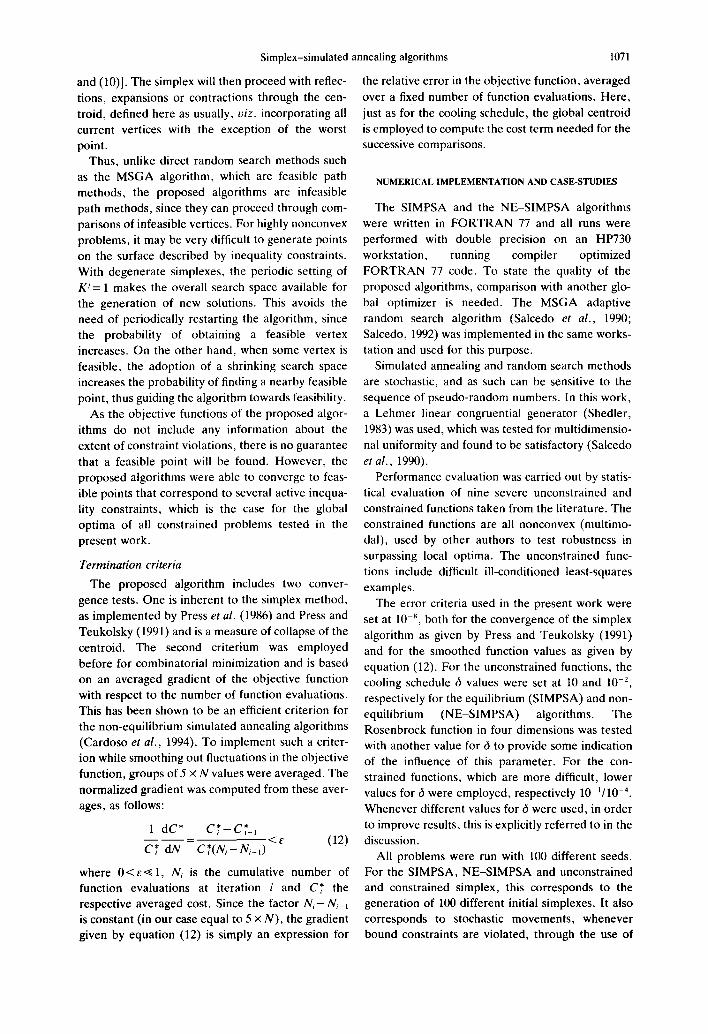
Table 3. Results for the unconstrained functions 1-5 (d = 10 for SIMPSA and d = 10 2 for NE-SIMPSA)

Starting Search MSGA Simplex SIMPSA NE-SIMPSA Function point interval Nsuc~* Ns .... Nf,,hjt Nsu~ N/,,bi Nsu~ N/,,h j

la - 1.2, 1) r [ - 1.2, 1.2] 100 100 323 100 10780 100 4508 [ - 10, 10] 100 100 352 1(81 12500 100 51107 [ - 100, 100] 98 100 394 99 13446 100 5353

Average: 9_.? 100 1_~ 10()

lb - 1.2, 1, - 1.2, 1) r 1- 1.2, 1.2] 100 96 938 99 21177 94 3053 10(1 43573:~ 99 17886~c

[ - 111, 10] 100 78 959 96 23616 82 3191 97 48282~: 89 18338~c

[ - 100, 100] 70 73 1025 82 25046 74 3421 93 528615 84 20061):~

Average: ~ 82 95 87

2 ( - 3 , - 1, -3 , - I) r 2*ABS(0) 81 10(I 11112 100 27483 100 3591 [ - 3, 31 100 99 1136 100 22615 100 3591

local optimum§ 2*ABS(()) 99 10t) 930 100 24675 10() 3493 local optimumll 2*ABS(0) 100 100 948 100 24830 100 3443 ( - 9, - 3, - 9, - 3) r 2*ABS(O) 78 100 1162 100 28201 100 3769

Average: 92 1~ 100 100

3 ( - 2 . . . . . - 2) 7- 2*ABS(0*) 27 92 95119 97 73115 91 9792 local optimum¶ [-0.5, 3.51 46 96 9249 93 56513 94 8613

[ - 0.3, 3.71 55 84 8435 93 54860 92 8099 (2 . . . . . 2) r [ - 0.5, 3.5] 44 79 6144 92 55089 77 6428

10, 4] 98 65 5565 93 52556 65 5882 Average: 54 83 94 84

4 (0.02, 4000, 250) r 2*ABS(0*) 4( < F= 176) 98 2569 92 19162 99 4426 ABS(0*) 5(<F= 176) 100 2586 99 18570 99 4424

5 (1, 1, 1, 2, 1,3) r 2*ABS(8*) 49( < F= 10 5) 100 3094 1 12913 99 6124

* Percent number of successes. "t Average number of function evaluations. ¢ d = 1 for SIMPSA and d = 10 3 for NE-SIMPSA § Local optimum = ( - 0.79633, 0.645242, 1.13839, 1.29675)1; F= 3.33443. [I Local optimum = (1, 1, - 0.94032, 0.89566)r; F= 3.886615. ¶ Local optimum = (0.94177, 0.88658, 0.77885, 0.59291, 0.35278, 0.12024, 0.031941, 0.0014266, -0.016515, 0.50500)r; F=0.504.

r e spec t ive ly , fo r t he s implex , N E - S I M P S A , r e p o r t e d in t he p r e s e n t work . T h e adap t ive r a n d o m

S I M P S A and M S G A a lgor i thms . Wi th fou r d i m e n - sea rch m e t h o d t e s t ed by these au t ho r s (Masr i et a l . ,

s ions a n d fou r la rge sea rch in te rva ls , all a lgo r i t hms 1980; P r o n z a t o et a l . , 1984) also r e q u i r e d m u c h

d e c r e a s e d in r o b u s t n e s s in ar r iv ing at the g lobal m o r e func t ion eva lua t ions wi th fou r d i m e n s i o n s

o p t i m u m of (1, 1, 1, 11 r. T h e S I M P S A a lgo r i thms than the M S G A a lgor i thm, a lbei t s ta r t ing f r o m

p r o d u c e d b e t t e r resul ts wi th sma l l e r va lues of t he d i f f e ren t so lu t ion vec to r s t han t h o s e e m p l o y e d he re .

coo l ing p a r a m e t e r d , bu t at a g r e a t e r e x p e n s e in Fo r func t ion 2, all a lgo r i t hms p e r f o r m e d wel l , bu t

c o m p u t a t i o n a l b u r d e n . T h e ave rage execu t ion t imes especia l ly again the s implex and the N E - S I M P S A

w e r e 0.46 s, 0.53 s, 1.46 s and 1.70 s, r e spec t ive ly , a lgo r i thms , s ince they r e q u i r e d m u c h f e w e r func t ion

for t he s imp lex , N E - S I M P S A , M S G A and S I M P S A eva lua t ions than the M S G A or S I M P S A a lgo r i thms ,

a lgo r i t hms , a n d i n c r e a s e d to 1 .52s and 3 . 0 0 s wi th and a lways a r r ived at t he global o p t i m u m . T h e

the s lower coo l ing s chedu le , r espec t ive ly , for t he ave rage execu t ion t imes w e r e 0.35 s, 0.42 s, 1 .28s

N E - S I M P S A a n d S I M P S A a lgor i thms . T h e non- and 1 .41s , respec t ive ly , for t he s implex ,

equ i l i b r i um var ian t ( N E - S I M P S A ) r equ i r e s m u c h N E - S I M P S A , S I M P S A and M S G A a lgor i thms .

f e w e r f unc t i on eva lua t ions t han the or ig inal Fo r func t ion 3, the wors t a lgo r i t hm is the adap t ive

M e t r o p o l i s ve r s i on , wi th only a smal l d e c r e a s e in r a n d o m search m e t h o d , which , de sp i t e its gene ra l

r o b u s t n e s s . Fo r this p r o b l e m , it can be s t a t ed tha t r o b u s t n e s s , is he re sensi t ive to t he s ta r t ing so lu t ion

the s imp lex m e t h o d o f N e l d e r and M e a d (1965) is vec to r and search in terval . It shou ld be n o t e d tha t

a l m os t as r obus t as the o t h e r t h r e e a lgo r i t hms a n d this p r o b l e m has 10 d e g r e e s o f f r e e d o m and a

r e q u i r e s m u c h f e w e r func t ion eva lua t ions . C o r a n a et difficult local o p t i m u m [local o p t i m u m (6) in Tab le

al. (1987) a lso o b s e r v e d the eff ic iency o f the s imp lex 3]. Aga in , bo th the s implex and N E - S I M P S A algor-

m e t h o d c o m p a r e d to s imu la t ed annea l i ng for the i t hms r equ i r e m u c h f e w e r func t ion eva lua t ions t h a n

m i n i m i z a t i o n o f t he R o s e n b r o c k func t ions , t he S I M P S A a lgo r i thm, wi th only a small d e c r e a s e

H o w e v e r , the i r i m p l e m e n t a t i o n o f s imu la t ed in robus tnes s . T h e ave rage execu t ion t imes w e r e

a n n e a l i n g r e q u i r e d a b o u t 5 x 105 func t ion evalu- 1.07 s, 1.54 s, 3.15 s and 6.50 s, respec t ive ly , for the

a t ions in two d i m e n s i o n s and 1 . 2 x 106 in fou r s implex , N E - S I M P S A , M S G A a n d S I M P S A algor-

d i m e n s i o n s , o i l m u c h la rger va lues t han those i thms .


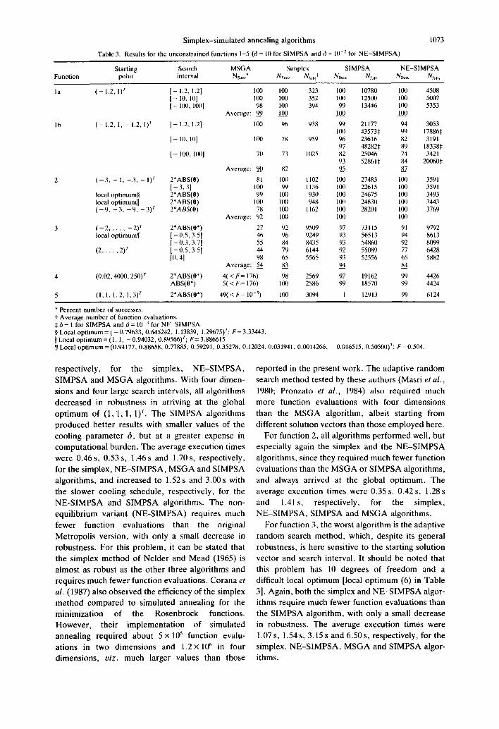
Table 4. Constrained functions

Global optimum Function Test function and constraints (author)

6 Luus (1974) y = O~ + O~ + 05 O~ = 0.988 4(01 - 0.5)-" + 2(0_,- 0.2) 2 + 0!:~+ O. 10 tO2 + 0.2020~ ~< 16 02 = 2.674 20] + 03- 20~ >~ 2 03 = - 1.884 -2.3~0i~<2.7 i=1,2 F= 11.67664

7 Luus and Jaakola (1973) Fuel allocation to power plants y = f~ 03 + g~ 04 O~ = 3(I

fj = 1.4609 + 0.151860j + 0.001450i 02 = 50 - 01 02 = 20 gj =0.8008+0.203102+0.00091602 18~<0L~<30 0:~ = () f2 = 1.5742 + 0.163101 + 0.0013580~ 14<~0~<25 04=0.58366 g2 = 0.7266 + 0.225602 + 0.0007780~ 0 ~< 03 <~ 1 F = 3.0521

0 < ~ 0 4 ~ < 1 (1 -- 03 ) f2 + (1 - 04)g2 ~ < 10

8 Luus (1975) Cross-extraction problem*

9 Grossman and Sargent (1979) Optimization of multicrudc pipeline~-

* A complete description is availabe in Luus (1975) or Salcedo et al. (1990). t A complete description is available in Grossmann and Sargent (1979).

Functions 4 and 5 represent least-squares struc- From the above discussion, we conclude that the

tures. It is well known that for this class of problems, simplex and N E - S I M P S A algorithms give more

it is strongly recommended to employ consistent results in arriving at the global opt imum.

Gauss-Newton- type methods. These functions are Also, as expected, the simplex required fewer func-

included in the present set of tests since they repre- tion evaluations. Comparing the equilibrium and

sent very ill-conditioned problems, non-equil ibrium versions of the simulated annealing

Function 4 is extremely ill condit ioned, since var- algorithms, the latter is much faster and generally as

iations of only 0.01% in each parameter , centered robust as the equilibrium version.

around the global opt imum, produce variations of Constrained optimization several orders of magnitude in the objective func-

tion. Actually, the opt imum parameter values Constrained optimization problems are more

reported for this function, as truncated and listed in interesting and probably more important than the

Table 2, produce a value of 2017 for the objective unconstrained ones, at least from the point of view

function, instead of the reported value of 88. Thus, of process engineering. Table 4 lists for four cases,

results within 100% of the global opt imum, viz. problems 6-9, selected for the present analysis. It

F < 176 are indeed acceptable. It can be seen that further includes the functional expressions for prob-

the simplex and N E - S I M P S A algorithms are very lems 6 and 7. Problems 8 and 9 are described in

efficient in solving this least-squares problem. The more detail later in the text. The simplex method,

average execution times were 0.44s, 0.71s, 1.81s and which was originally developed for unconstrained

3.26 s, respectively, for the simplex, N E - S I M P S A , problems, was modified according to the method

SIMPSA and M S G A algorithms, given above (under the section entitled Dealing with

For function 5, a triple exponential , even more constraints) and as such can be directly compared

difficult to fit, the worst results occur with the with the other algorithms. The only algorithmic

S IMPSA algorithm, which only produced one objec- difference between the constrained simplex algor-

tive function below 10 -5, whereas the N E - S I M P S A ithm and the SIMPSA and N E - S I M P S A algorithms

and the simplex algorithms produced much more is that, in the former, the temperature is always

accurate results. The forced decrease in temperature equal to zero, which deactivates the simulated

in the N E - S I M P S A version approximates the algor- annealing scheme. Obviously, the shrinking effect

ithm to the original simplex method, whereas the on the size of the region centered on the current best equil ibrium version wanders in the search domain vertex following the cooling schedule, given by

witout being able to significantly decrease the objec- equation (11), is not applicable here, since the

tive function. The behavior of the M S G A algorithm temperature remains always at zero.

is somewhere between these two extremes. As seen Table 5 shows the results obtained by all algor-

in Table 3, all algorithms performed better with a ithms in solving function 6. Here , the constrained

smaller search region. The average execution times simplex algorithm is the worst, and the SIMPSA

were 2.17s, 5.17s, 8.62s and 21.9s, respectively, variants the best, the non-equilibrium version

for the simplex, N E - S I M P S A , SIMPSA and M S G A requiring about half the number of function evalu-

algorithms, ations for only a small decrease in robustness. The


MSGA algorithm requires more function evalu- The equilibrium curves for the solute on both phases ations than either the SIMPSA or NE-SIMPSA are given by Luus (19751 as two cubics: implementations, and produces somewhat poorer y=2 .50x + 3 .70x2-113 .0x 3 x<~0.1 (13) results. The average execution times were 0.28s, 1.00s, 1.20s and 1.70s, respectively, for the sim- y = 3 . 9 4 x - 2 9 . 6 x 2 + 7 4 . 0 x 3 x>0 .1 . (14)

plex, NE-SIMPSA, MSGA and SIMPSA algor- Assuming a known feed rate Q and the maximum ithms, allowable extraction, the process has five degrees of

Table 6 shows the average number of function freedom. The objective function is: evaluations required by all algorithms to solve func-

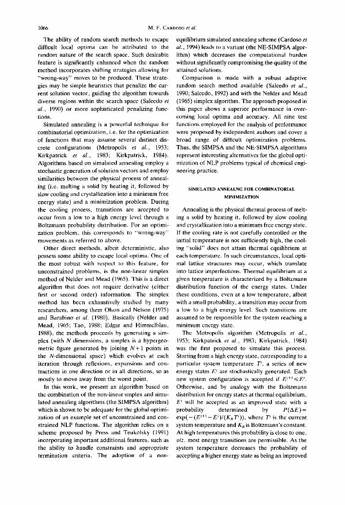
max F = {Q(x~- xl) - )~(wt + w2 + w3) tions 7-9. Figures la and lb show the behavior of all algorithms for the optimization of the fuel allocation - C[f~wl +f2(w~f~ + w2)]} (15)

problem (function 7), respectively for the two differ- where 2 is the relative cost of the extraction solvent ent starting points given in Table 6. These figures W (i.e. cost of unit of solvent W per unit of value of show the number of trials (out of 100 runs) which extracted product) and C is the relative cost of reached a value of the objective function within a recycling (i.e. cost of unit recycled per unit of value percentage of the global optimum. As this function of extracted product). The five decision variables exhibits local minima which are about 0.5-1% of the are {f~, f2, x~, w~, w21, subject to: global optimum, the results indicate that the SIMPSA, NE-SIMPSA and MSGA algorithms 0~<f~<l; i = 1 , 2 (16)

were all robust in solving this problem, the non- 0~<xt~ < (Xf)ma x (17) equilibrium algorithm requiring about one half the 3 number of function evaluations as compared to the 0 ~ < ~ wi~ < CAP (18) equilibrium version. Also, the simplex algorithm is i-

very sensitive to the starting point, in opposition to 0 ~ < wi; i = 1-3 ((19) what occurs with the other three algorithms. The

where the value of (Xf)m,x and CAP depend on the average execution times were 0.28 s, 1.34 s, 1.49 s and 2.59 s, respectively, for the constrained simplex, particular data. The pertinent data used are shown

in Table 7. Also shown are the global optima for MSGA, NE-SIMPSA and SIMPSA algorithms.

both cases, determined with the MSGA algorithm through optimized tunning of the search grids (Sal-

The classical cross-extraction problem cedo et al., 1990). The objective function for case 1 exhibits one local optimum at {f~, f~_, xj, w~, w2;

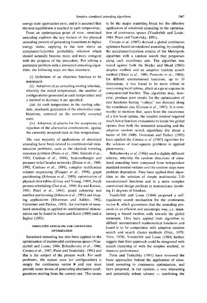
This problem is given by Luus (1975) and was F}={1, 0, 0.0257795, 0.4945684, 0; 0.1111452}, extensively tested by Salcedo et al. (1990). It is a which is only about 0.25% lower than the global very good example of a simple chemical engineering optimum. On the other hand, the objective function process and a challenge to an optimization algorithm for case 2 is rather insensitive to the optimization due to the presence of difficult local optima. Figure parameters, with widely different values of the inde- 2 is a schematic diagram of the process, where the pendent parameters producing values within 1% of solvents Q and W are totally immiscible and f, the global optimum. This combination of multimo- represents the fraction recycled from stage i to stage dality and rippled search surface makes the problem i + 1. The xs and ys represent mass fractions of challenging and the global optimum difficult to solute, respectively, on solvent phases Q and W. arrive at.

Table 5. Results for the constrained function 6 (b = 10 ] for S IMPSA and 6 = 10 ~ for N E - S I M P S A )

M S G A Simplex S I M P S A N E - S I M P S A Start ing point Nsu~* Nsuc~ N/~,hjt Nsu~ N/~,h j Nsu~¢ N/~,~ i

(1.04400, 2.48909, 1.78541) t 87 0 511 100 31950 95 167112 (2.22288, - 0.17259, 1.98899) t 71 11 624 100 31500 96 15742 (1.57411, - 1.79381, - 1.75688) ~ 70 0 531 99 31588 87 15352 (2.04195, - 0.95967, - 1.90526) ~ 78 4 577 99 31626 94 15575 ( - 1.41862, - 0 . 1 6 0 5 0 , 1.01260) T 76 32 943 98 29915 96 15714 (1.40498, - 0.24513, - 1.002001 r 76 18 942 100 31195 92 15779 ( - 1.3, - 0 . 3 , 0.63) 1 75 29 958 96 311516 90 14610

Average 7_._66 13 99 9...33

* Percent number of successes. t Ave rage number of function evaluations.

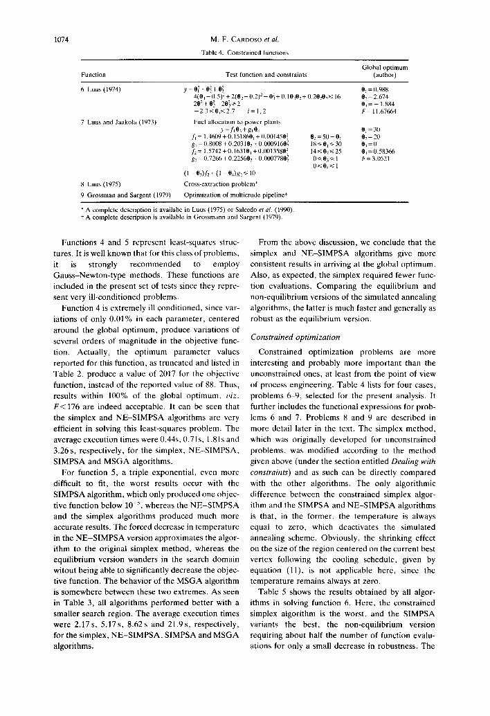
1076 M.F. CARDOSO et al. Table 6. Average number of objective function evaluation (100 runs) for the con-

strained functions 7-9 (b= l0 -l for SIMPSA and 6 = 10 4 for NE-SIMPSA)

Function Starting point Simplex S IMPSA NE-SIMPSA

7 (25, 1, 1) r 845 44413 23839 (3t). o, 0.6) r 631 44622 24651

8 (1, 1, 1, 0.3, o) T 954 59842 23970 (0, 0, 0.3, 1.2, o) r 1546 46734 23214

9 (28.14, 14, 110, 110, 110, 110) T 2040 524112 13780 298228* 60037*

* b= to-: for SIMPSA and ~ = 10 5 for NE-SIMPSA.

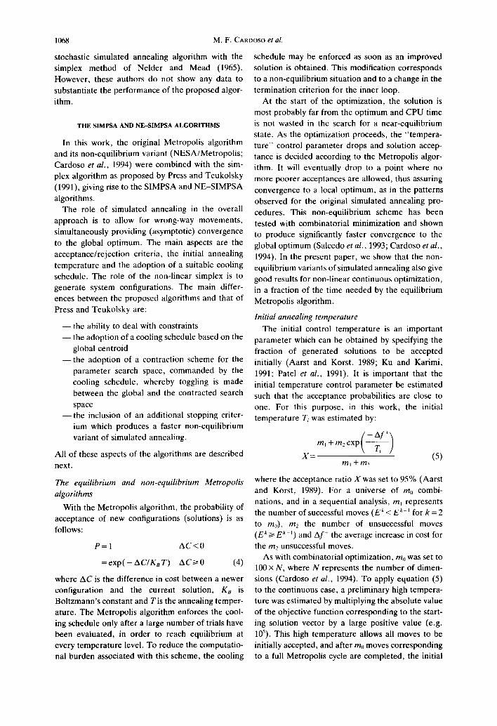
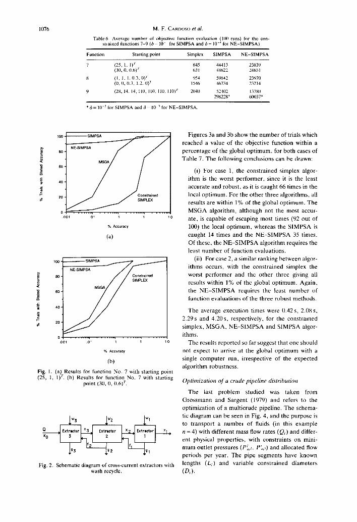
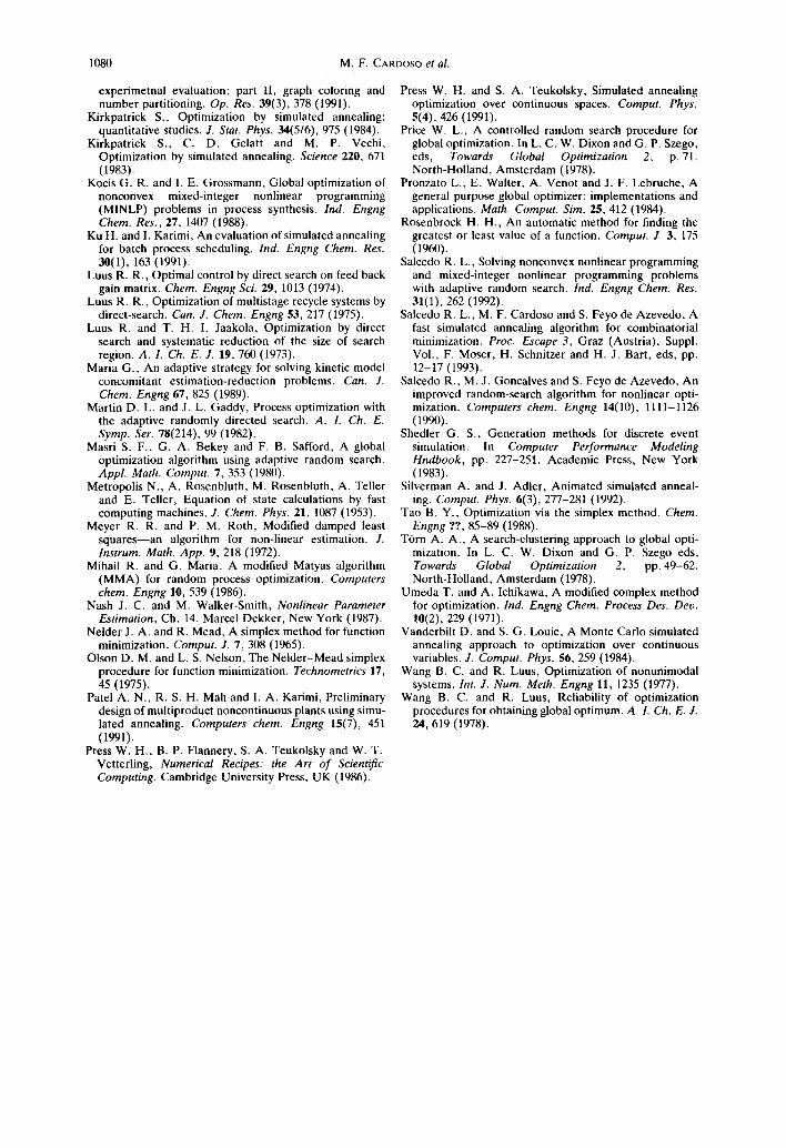
SIMPSA Figures 3a and 3b show the n u m b e r of trials which 100 ~ ~ reached a value of the object ive funct ion within a

~NE-SIMPSA / / ~" 80 percen tage of the global op t imum, for bo th cases of

< Table 7. The following conclusions can be drawn:

(i) For case 1, the cons t ra ined simplex algor-

= i thm is the worst pe r fo rmer , since it is the least

accurate and robust , as it is caught 66 t imes in the

.~ 20 J J Constrained local op t imum. For the o ther th ree a lgori thms, all j ~ SIMPLEX results are within 1% of the global op t imum. The

o - - . . . . . . . . . . . . . . . . . . . . . . . . . . . . . . . . . . . M S G A algor i thm, a l though not the most accur- .00t 01 .t 1 t0 ate, is capable of escaping most t imes (92 out of

% Ascuraoy 100) the local op t imum, whereas the S I M P S A is

(a) caught 14 t imes and the N E - S I M P S A 35 times.

Of these, the N E - S I M P S A algor i thm requires the

least n u m b e r of funct ion evaluat ions .

100" SIMPSA ~ . . . . . ~ f . . ~ (ii) For case 2, a similar ranking be tween algor-

NE-SIMPSA j / i thms occurs, with the cons t ra ined simplex the

80- f / Constrained worst pe r fo rmer and the o the r three giving all / / SIMPLEX results within 1% of the global op t imum. Again ,

60. M S C ~ / / the N E - S I M P S A requires the least n u m b e r of

~ funct ion evaluat ions of the three robust methods . .1=

~ 40 The average execut ion t imes were 0.42 s, 2.08 s,

~- 2.29 s and 4.20 s, respectively, for the cons t ra ined 20"

simplex, M S G A , N E - S I M P S A and S IMPSA algor-

i thms. 0 . . . . . . . . i . . . . . . . . i . . . . . . . . i . . . . . . . . .0ol .01 .t t 0 The results repor ted so far suggest tha t one should

% Accuracy not expect to arrive at the global op t imum with a

(b) single compu te r run, i rrespective of the expected

a lgor i thm robustness . Fig. l. (a) Results for function No. 7 with starting point (25, 1, 1) r. (b) Results for function No. 7 with starting

point (30, 0, 0.6) r. Optimization of a crude pipeline distribution

The last p rob lem studied was taken from

G r o s s m a n n and Sargent (1979) and refers to the

opt imizat ion of a mul t icrude pipeline. The schema-

~ 1 ~ 3 vz ~ ' ~ 1 tic d iagram can be seen in Fig. 4, and the purpose is J, to t ranspor t a n u m b e r of fluids (in this example

O I ~ 2 Fxtraetor ~ x z xl 4) with different mass flow rates (Qi) and differ- x 0 2 I, n =

ent physical proper t ies , with const ra in ts on mini-

l (P.,_,, and al located flow ,LY3 ~z mum outlet pressures i P',,,~) periods per year. The pipe segments have known

Fig. 2. Schematic diagram of cross-current extractors with lengths (L~) and variable cons t ra ined d iameters wash recycle. (Di).


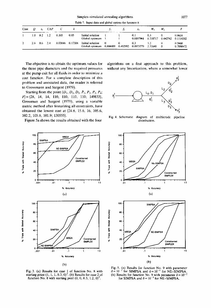
Table 7. Input data and global optima for function 8

Case Q X¢ CAP C 2 fl ]'2 xt Wi W2 F

1 I.[1 I).2 1.2 0.105 0.05 Initial solution 1 1 0.1 0.3 0 0.0624 Globaloptimum 1 1 0.0197961 0.318717 0.442742 0.1114302

2 2.6 0.6 2.4 0.03846 0.17308 Initial solution 0 0 0.3 1.2 0 0.5668 Global optimum 0.886009 0.492992 0.0973779 2.31640 0 0.7880472

The objec t ive is to ob ta in the op t i m um values for a lgor i thms on a first approach to this p rob lem,

the th ree pipe d iamete r s and the requi red pressures wi thout any l inear izat ion, where a somewha t lower

at the p u m p exit for all fluids in o rder to minimize a

cost funct ion. For a comple te descr ipt ion of this F i

p rob lem and associated data , the reader is re fer red o 2 / ~ 2 to G r o s s m a n n and Sargent (1979). ~

Star t ing f rom the poin t {D~, D2, D3, P~, P2, P3, P4; . f " - ~ k 1, O 1 F}={28, 14, 14, 110, 110, 110, 110; 149833}, F] ~ Q~ G r o s s m a n and Sargent (1979), using a var iable t - ~ 3

metr ic m e t h o d af ter l inearizing all constra ints , have DD3~ -

obtained the lowest cost at {24.6, 15.6, 16, 105.6,

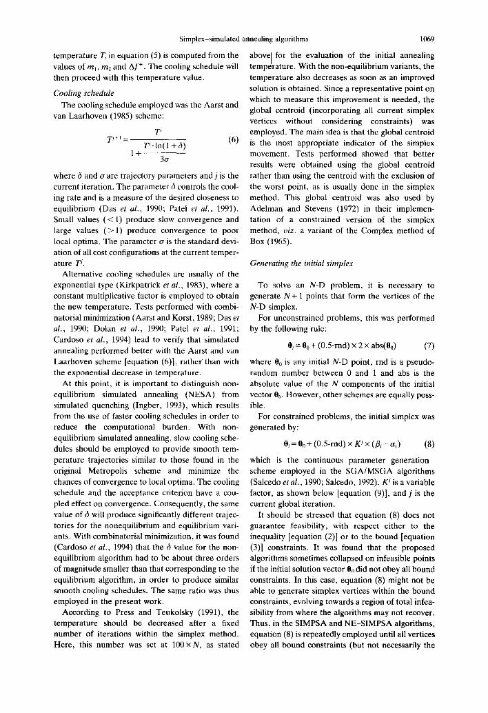
102.2, 105.6, 101.9; 130555}. Fig. 4. Schematic diagram of multicrude pipeline Figure 5a shows the results ob ta ined with the four distribution.

100 f 100 ,~ 80 ~ 80

8 ° <

ed J:: ~=

3= 40 - ~ 40 NE-SIMPSA

20 - ~ 20 ed

0 . . . . . . . . i . . . . . . . . i . . . . . . . . i . . . . . . . . 0 i . . . . . . . . i . . . . . . . . i . . . . . . . . .OOt .01 .1 1 0 .01 . I 1 1 0

% Accuracy % Accuracy

(a) Ca)

100 • ~ 100

60. ~ 6o

J¢ J= g= 40 ' ~ 40

~" j / ~ MSGA / Constrained ;.C. --EX

0 0 .001 . . . . . . . . ,01' . . . . . . . . . . . . . . . . . . . . . . . . 1 ' 1 0 I .01 .I I 10

% Accuracy % Accuracy

(b) (b)

Fig. 5. (a) Results for function No. 9 with parameter Fig. 3. (a) Results for case 1 of function No. 8 with di= 10-1 for SIMPSA and ~ = 10 4 for NE-SIMPSA. starting point (1, 1, 1, 0.3, 0) r. (b) Results for case 2 of (b) Results for function No. 9 with parameter b = 10 -2

function No. 8 with starting pont (0, 0, 0.3, 1.2, 0) r. for SIMPSA and b = 10 -5 for NE-SIMPSA.


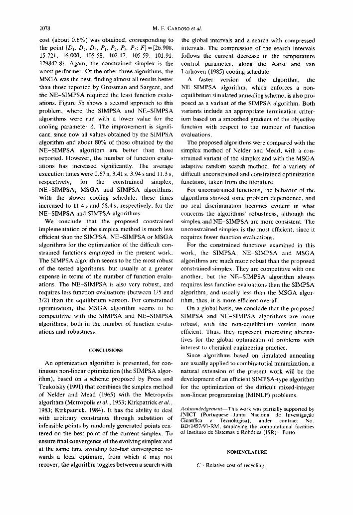
cost (about 0.6%) was obtained, corresponding to the global intervals and a search with compressed the point {Dr, D2, D3, P~, P2, P3. P4; F}={26.908, intervals. The compression of the search intervals 15.221, 16.000, 105.58, 102.17, 105.59, 101.91; follows the current decrease in the temperature 129842.8}. Again, the constrained simplex is the control parameter, along the Aarst and van worst performer. Of the other three algorithms, the Larhoven (1985) cooling schedule. MSGA was the best, finding almost all results better A faster version of the algorithm, the than those reported by Grossman and Sargent, and NE-SIMPSA algorithm, which enforces a non- the NE-SIMPSA required the least function evalu- equilibrium simulated annealing scheme, is also pro- ations. Figure 5b shows a second approach to this posed as a variant of the SIMPSA algorithm. Both problem, where the SIMPSA and NE-SIMPSA variants include an appropriate termination criter- algorithms were run with a lower value for the ium based on a smoothed gradient of the objective cooling parameter 6. The improvement is signifi- function with respect to the number of function cant, since now all values obtained by the SIMPSA evaluations. algorithm and about 80% of those obtained by the The proposed algorithms were compared with the NE-SIMPSA algorithm are better than those simplex method of Nelder and Mead, with a con- reported. However, the number of function evalu- strained variant of the simplex and with the MSGA ations has increased significantly. The average adaptive random search method, for a variety of execution times were 0.67 s, 3.41 s, 3.94 s and 11.3 s, difficult unconstrained and constrained optimization respectively, for the constrained simplex, functions, taken from the literature. NE-SIMPSA, MSGA and SIMPSA algorithms. For unconstrained functions, the behavior of the With the slower cooling schedule, these times algorithms showed some problem dependence, and increased to 11.4s and 58.4s, respectively, for the no real discrimination becomes evident in what NE-SIMPSA and SIMPSA algorithms, concerns the algorithms' robustness, although the

We conclude that the proposed constrained simplex and NE-SIMPSA are more consistent. The implementation of the simplex method is much less unconstrained simplex is the most efficient, since it efficient than the SIMPSA, NE-SIMPSA or MSGA requires fewer function evaluations. algorithms for the optimization of the difficult con- For the constrained functions examined in this strained functions employed in the present work. work, the SIMPSA, NE-SIMPSA and MSGA The SIMPSA algorithm seems to be the most robust algorithms are much more robust than the proposed of the tested algorithms, but usually at a greater constrained simplex. They are competitive with one expense in terms of the number of function evalu- another, but the NE-SIMPSA algorithm always ations. The NE-SIMPSA is also very robust, and requires less function evaluations than the SIMPSA requires less function evaluations (between 1/5 and algorithm, and usually less than the MSGA algor- 1/2) than the equilibrium version. For constrained ithm, thus, it is more efficient overall. optimization, the MSGA algorithm seems to be On a global basis, we conclude that the proposed competititve with the SIMPSA and NE-SIMPSA SIMPSA and NE-SIMPSA algorithms are more algorithms, both in the number of function evalu- robust, with the non-equilibrium version more ations and robustness, efficient. Thus, they represent interesting alterna-

tives for the global optimizatin of problems with interest to chemical engineering practice. CONCLUSIONS

Since algorithms based on simulated annealing An optimization algorithm is presented, for con- are usually applied to combinatorial minimization, a

tinuous non-linear optimization (the SIMPSA algor- natural extension of the present work will be the ithm), based on a scheme proposed by Press and development of an efficient SIMPSA-type algorithm Teukolsky (1991) that combines the simplex method for the optimization of the difficult mixed-integer of Nelder and Mead (1965) with the Metropolis non-linear programming (MINLP)problems. algorithm (Metropolis et al . , 1953; Kirkpatrick et al. , 1983; Kirkpatrick, 1984). It has the ability to deal Acknowledgement- -This work was partially supported by

JNICT (Portuguese Junta Nacional de Investiga~o with arbitrary constraints through substition of Cientifica e Tecnol6gica), under contract No. infeasible points by randomly generated points cen- BD/1457/91-RM, employing the computational facilities tered on the best point of the current simplex. To of Instituto de Sistemas e Rob6tica (ISR)--Porto.

ensure final convergence of the evolving simplex and at the same time avoiding too-fast convergence tO- NOMENCLATURE wards a local optimum, from which it may not recover, the algorithm toggles between a search with C = Relative cost of recycling


C* = Cost average over a fixed number of function Adeiman A. and W. F. Stevens, Process optimization by evaluations the Complex method. A. L C h . E . J. 18(1), 20 (1972).

AC=Dif fe rence in cost between new and current Barabino G. P., G. S. Barabino, B. Bianco and M. configurations Marchesi, A study on the performance of simplex meth-

C A P = Restriction on allowable solvent rates (Kg/h) ods for function minimization. Proc. IEEE Int. Conf. Di = Pipe diameter (m) Circuits Comput. 1CCC 80, 150-1153. IEEE, New York E j = Energy state of system configuration j (1980).

AE=Di f fe rence in energy between new and current Bohachevsky I. O., M. E. Johnson and M. L. Stein, configurations Generalized simulated annealing for function optimiza-

F = Objective function tion. Technometrics 28(3), 209 (1986). f, = Recycled fraction from extractor i to i + 1, Box M. J., A new method of constrained optimization and

i = 1-2 a comparison with other methods. Computer J. 8, 42 Af ÷ = Average increase in cost for the m2 unsuccess- (1965).

ful moves Campbell J. R. and J. L. Gaddy, Methodology for simulta- gj = Inequality constraint, j = 1-m neous optimization with reliability: nuclear PWR exam-

Ka = Boltzmann's constant pie. A. 1. Ch.E. J. 22(6), 1050 (1976). KJ=Variable compression factor at iteration j Cardoso M. F., R. L. Salcedo and S. F. de Azevedo, Li = Pipe length (m) m = Number of inequality constraints Non-equilibrium simulated annealing: a faster approach

rn~ = Number of successful moves to combinatorial minimization. Ind. Engng Chem. Res. m2 = Number of unsuccessful moves 33(8), 1908 (1994).

Colville A. R., A comparative study of non-linear pro- N = Number of independent parameters Ni = Cumulative number of function evaluations at gramming codes. IBM N.Y. Scientific Center, T.R. 320-

iteration i 2925 (1968). P = Probability of acceptance/rejection of current Corana A., M. Marchesi, C. Martini and S. Ridella,

solution Minimizing multimodal functions of continuous vari- / ) ,=Outle t pressure of pipe i (Pa) ables with the simulated annealing algorithm. ACM

P~j = Minimum outlet pressures of pipe j with fluid i Trans. Math. Software 13(3), 263 (1987). (Pa) Corey E. M. and D. A. Young, Optimization of physical

Q = Mass feed rate to extraction system (kg/h) data tables by simulated annealing. Comput. Phys. 3(3), Q, = Mass flow rate of fluid i (kg/h) 33 (1989).

rnd = Pseudo-random number between 0 and 1 Das H., P. T. Cummings and M. D. Levan, Scheduling of TJ=System (annea l ing ) t empera tu reo f i t e ra t ion j serial mutliproduct batch processes via simulated w~ = Mass flow rate of wash solvent (Kg/h) to annealing. Computers chem. Engng 14(12), 1351 (1990).

extractor i, i= 1-3 Dolan W. B., P. T. Cummings and M. D. Levan, Process X = Acceptance ratio optimization via simulated annealing: application to Xr = Mass fraction of solute in feed network design. A. 1. Ch.E. J. 35(5), 725 (1989). x ,=Mass fraction of solute in outlet from extrac- Dolan W. B., P. T. Cummings and M. D. Levan,

tor i, i= 1-3 Algorithmic efficiency of simulated annealing for heat y~= Mass fraction of solute in wash current exchanger network design. Computers chem. Engng

(extractor i), i = 1-3 14(10), 1039 (1990).

Greek symbols Dixon L. C. W., Conjugate directions without linear searches. J. Ins. Math. Appl. 11,317 (1973).

a i= Lower bound on parameter i, i = 1-n Edgar T. F. and D. M. Himmelblau, Optimization of fli = Upper bound on parameter i, i = 1-n Chemical Processes. McGraw-Hill, New York (1988). 6 =Cooling rate control parameter Floquet P., L. Pibouleau and S. Domenech, Separation e = Error criterion (relative) 2=Rela t ive cost of extraction solvent sequence synthesis: how to use simulated annealing o = Standard deviation of all cost functions at cur- procedure. Computers chem. Engng 18(11/12), 1141

(1994). rent temperature

0 = V e c t o r of independent parameters Floudas C. A., A. Aggarwal and A. R. Ciric, Global 0* = Initial solution vector optimum search for nonconvex NLP and MINLP prob-

lems. Computers chem. Engng 13(10), 1117 (1989). Abbreviations Gaines L. D. and J. L. Gaddy, Process optimization by

CEP = Chemical engineering problems flow sheet optimization. Ind. Eng. Chem. Process Des. CMAX = Constrained maximization problems Dev. 15,206 (1976). CMIN = Constrained minimization problems Groisman G. and J. R. Parker, Computer-assisted photo-

SGA=Sa lcedo -Gonqa lves -Azevedo algorithm metry using simualted annealing. Comput. Phys. 7(1), MSGA = Minlp Salcedo-Gonqalves-Azevedo algorithm 87 (1993). MINLP = Mixed integer non-linear programming Grossmann I. E. and R. W. H. Sargent, Optimal design of

NLP=Non- l inea rprogramming multipurpose chemical plants. Ind. Engng Chem. ULS = Unconstrained least-squares problems Process Des. Dev. 18, 343 (1979).

UMIN = Unconstrained minimization problems Heuckroth M. W., J. L. Gaddy and L. D. Gaines, An examination of the adaptive random search technique.

R E F E R E N C E S A. 1. Ch.E. J. 22, 744 (1976). Ingber A. L., Simulated annealing: practice versus theory.

Aarst E. and J. Korst, Similated Annealing and Boltzmann J. Math. Comput. Modelling 18(11), 29 (1993). Machines--a Stochastic Approach to Combinatorial Johnson D. S., C. R. Aragon, L. A. McGeoch and C. Optimization and Neural Computers. Wiley, New York Schevon, Optimization by simulated annealing: an (1989). experimental evaluation; part I, graph partitioning. Op.

Aarst E. H. L. and P. J. M. van Laarhoven, Statistical Res. 37(6), 865 (1989). cooling: a general approach to combinatorial optimiza- Johnson D. S., C. R. Aragon, L. A. McGeoch and C. tion problems. Philips J. Res. 40, 193 (1985). Schevon, Optimization by simulated annealing: an


experimetnal evaluation; part 11, graph coloring and Press W. H. and S. A. Teukolsky, Simulated annealing number partitioning. Op. Res. 39(3), 378 (1991). optimization over continuous spaces. Comput. Phys.

Kirkpatrick S., Optimization by simulated annealing: 5(4), 426 (1991). quantitative studies. J. Star. Phys. 34(5/6), 975 (1984). Price W. L., A controlled random search procedure for

Kirkpatrick S., C. D. Gelatt and M. P. Vechi, global optimization. In L. C. W. Dixon and G. P. Szego, Optimization by simulated annealing. Science 220, 671 eds, Towards Global Optimization 2, p. 71. (1983). North-Holland, Amsterdam (1978).

Kocis G. R. and I. E. Grossmann, Global optimization of Pronzato L., E. Walter, A. Venot and J. F. Lebruche, A nonconvex mixed-integer nonlinear programming general purpose global optimizer: implementations and (MINLP) problems in process synthesis. Ind. Engng applications. Math. Comput. Sire. 25,412 (1984). Chem. Res., 27, 1407 (1988). Rosenbrock H. H., An automatic method for finding the

Ku H. and I. Karimi, An evaluation of simulated annealing greatest or least value of a function. Comput. J. 3, 175 for batch process scheduling. Ind. Engng Chem. Res. (1960). 30(1), 163 (1991). Salcedo R. L., Solving nonconvex nonlinear programming

Luus R. R., Optimal control by direct search on feed back and mixed-integer nonlinear programming problems gain matrix. Chem. Engng Sci. 29, 1013 (1974). with adaptive random search. Ind. Engng Chem. Res.

Luus R. R., Optimization of multistage recycle systems by 31(1), 262 (1992). direct-search. Can. J. Chem. Engng 53, 217 (1975). Salcedo R. L., M. F. Cardoso and S. Feyo de Azevedo, A

Luus R. and T. H. I. Jaakola, Optimization by direct fast simulated annealing algorithm for combinatorial search and systematic reduction of the size of search minimization. Proc. Escape 3, Graz (Austria), Suppl. region. A. 1. Ch.E. J. 19, 760 (1973). Vol., F. Moser, H. Schnitzer and H. J. Bart, eds, pp.

Maria G., An adaptive strategy for solving kinetic model 12-17 (1993). concomitant estimation-reduction problems. Can. J. Salcedo R., M. J. Goncalves and S. Feyo de Azevedo, An Chem. Engng 67,825 (1989). improved random-search algorithm for nonlinear opti-

Martin D. L. and J. L. Gaddy, Process optimization with mization. Computers chem. Engng 14(10), 1111-1126 the adaptive randomly directed search. A. 1. Ch. E. (1990). Syrup. Set. 78(214), 99 (1982). Shedler G. S., Generation methods for discrete event

Masri S. F., G. A. Bekey and F. B. Safford, A global simulation. In Computer Performance Modeling optimization algorithm using adaptive random search. Hndbook, pp. 227-251. Academic Press, New York Appl. Math. Comput. 7, 353 (1980). (1983).

Metropolis N., A. Rosenbluth, M. Rosenbluth, A. Teller Silverman A. and J. Adler, Animated simulated anneal- and E. Teller, Equation of state calculations by fast ing. Comput. Phys. 6(3), 277-281 (1992). computing machines. J. Chem. Phys. 21, 1087 (1953). Tao B. Y., Optimization via the simplex method. Chem.

Meyer R. R. and P. M. Roth, Modified damped least Engng ??, 85-89 (1988). squares--an algorithm for non-linear estimation. J. TOrn A. A., A search-clustering approach to global opti- lnstrum. Math. App. 9, 218 (1972). mization. In L. C. W. Dixon and G. P. Szego eds,

Mihail R. and G. Maria, A modified Matyas algorithm Towards Global Optimization 2, pp. 49-62. (MMA) for random process optimization. Computers North-Holland, Amsterdam (1978). chem. Engng 10, 539 (1986). Umeda T. and A. Ichikawa, A modified complex method

Nash J. C. and M. Walker-Smith, Nonlinear Parameter for optimization. Ind. Engng Chem. Process Des. Deo. Estimation, Ch. 14. Marcel Dekker, New York (1987). 10(2), 229 (1971).

Nelder J. A. and R. Mead, A simplex method for function Vanderbilt D. and S. G. Louie, A Monte Carlo simulated minimization. Comput. J. 7,308 (1965). annealing approach to optimization over continuous

Olson D. M. and L. S. Nelson, The Nelder-Mead simplex variables. J. Comput. Phys. 56, 259 (1984). procedure for function minimization. Technometrics 17, Wang B. C. and R. Luus, Optimization of nonunimodal 45 (1975). systems. Int. J. Num. Meth. Engng 11, 1235 (1977).

Patel A. N., R. S. H. Mah and I. A. Karimi, Preliminary Wang B. C. and R. Luus, Reliability of optimization design of multiproduct noncontinuous plants using simu- procedures for obtaining global optimum. A. 1. Ch. E. J. lated annealing. Computers chem. Engng 15(7), 451 24, 619 (1978). (1991).

Press W. H., B. P. Flannery, S. A. Teukolsky and W. T. Vetterling, Numerical Recipes: the Art of Scientific Computing. Cambridge University Press, UK (1986).

THE SIMPLEX-SIMULATED ANNEALING APPROACH...

Documents

Transcript of THE SIMPLEX-SIMULATED ANNEALING APPROACH...