The Shifting Gender Balance in Higher Education and ...
41
1 The Shifting Gender Balance in Higher Education and Assortative Mating in Europe Yolien De Hauw*, André Grow & Jan Van Bavel Centre for Sociological Research, University of Leuven, Leuven, Belgium Abstract While men have always received more education than women in the past, this gender imbalance in education has now turned around in most European countries. For the first time in history, there are more highly educated women than men reaching the reproductive ages and looking for a partner. This paper investigates implications for recent trends in educational assortative mating. To this end, we used pooled data from the European Social Survey (rounds 1-6) combined with country level education-specific sex ratios. Descriptive results point to a turnover from female educational hypergamy (women partnering up) to hypogamy (women partnering down) in just one generation. Multilevel regression analyses indicates that the reversal of gender inequality in education has been a driver of the change from hypergamy to hypogamy. The degree of educational homogamy, in contrast, is largely driven by own educational attainment as such, rather than by changes in education-specific sex ratios. Against our expectations, the reversal of the gender gap in education is not associated with highly educated women remaining single more often. Rather, it is highly educated men as well as low educated women who more often living single. Paper to be presented at the 2015 Annual Meeting of the Population Association of America, San Diego (CA), USA, April 30 – May 2, 2015. E-mails: [email protected]; André[email protected]; [email protected]
Transcript of The Shifting Gender Balance in Higher Education and ...

1
The Shifting Gender Balance in Higher Education and Assortative
Mating in Europe
Yolien De Hauw*, André Grow & Jan Van Bavel
Centre for Sociological Research, University of Leuven, Leuven, Belgium
Abstract
While men have always received more education than women in the past, this gender
imbalance in education has now turned around in most European countries. For the first time
in history, there are more highly educated women than men reaching the reproductive ages
and looking for a partner. This paper investigates implications for recent trends in educational
assortative mating. To this end, we used pooled data from the European Social Survey
(rounds 1-6) combined with country level education-specific sex ratios. Descriptive results
point to a turnover from female educational hypergamy (women partnering up) to hypogamy
(women partnering down) in just one generation. Multilevel regression analyses indicates that
the reversal of gender inequality in education has been a driver of the change from hypergamy
to hypogamy. The degree of educational homogamy, in contrast, is largely driven by own
educational attainment as such, rather than by changes in education-specific sex ratios.
Against our expectations, the reversal of the gender gap in education is not associated with
highly educated women remaining single more often. Rather, it is highly educated men as
well as low educated women who more often living single.
Paper to be presented at the 2015 Annual Meeting of the Population Association of America,
San Diego (CA), USA, April 30 – May 2, 2015.
E-mails: [email protected]; André[email protected];

2
Contents
1. Introduction ........................................................................................................................ 3
2. Theoretical background ...................................................................................................... 5
2.1 Martial search theory .................................................................................................... 6
2.2 Individual preferences and the role of education .......................................................... 7
2.3 The reversal of the gender imbalance in education and mating: Hypotheses ............... 8
3. Method .............................................................................................................................. 10
3.1 Analytical approach .................................................................................................... 10
3.2 Data ............................................................................................................................. 11
3.3 Measures ..................................................................................................................... 12
3.3.1 Dependent variables ................................................................................................. 12
3.3.2 Main independent variables ..................................................................................... 13
3.3.3 Control variables ...................................................................................................... 14
4. Results .............................................................................................................................. 15
4.1 Descriptive results ....................................................................................................... 15
4.2 Multilevel regression results ....................................................................................... 17
4.2.1 Singlehood ............................................................................................................... 17
4.2.2 Assortative mating ................................................................................................... 19
5. Conclusion and discussion ................................................................................................ 22
6. References ........................................................................................................................ 26
Appendix 1 ........................................................................................................................... 31
Tables and Figures ................................................................................................................ 33

3
1. Introduction
A major social development in the second half of the twentieth century has been the dramatic
increase of participation in higher education, in particular among women. One important
consequence of this development is that differences in the relative educational attainment of
men and women have changed: in the past, men were typically higher educated than women,
while today women excel men in terms of participation and success in higher education. This
holds for almost all European countries (Vincent-Lancrin, 2008), but also for North America
(Diprete & Buchmann, 2006) and many other parts of the world (Esteve, García-Román, and
Permanyer 2012; Schofer and Meyer 2005). This implies that today, for the first time in
history, there are more highly educated women than men reaching the reproductive ages.
Figure 1 charts the major turnaround that has occurred in the participation of men and women
in higher education for European countries, Canada, and the U.S.A. Using country codes as
symbols, the figure plots the percentage of female students among all students in tertiary
education. The upward trend is massive: while in 1971 only one country had reached gender
parity in higher education (Bulgaria, BG), a third of these countries had crossed the 50% line
by 1983. In 2009, all but one country (Switzerland, CH) had a female majority in higher
education. Iceland (IC) exhibited the most spectacular rise: in 1971, it had the lowest
proportion female of all countries included in the plot (25%), while it had the highest
proportion in 2009 (64%). Countries with similarly spectacular rises over this period include
Norway (30% to 60%), Denmark (37% to 58%), the UK (from 33% to 57%), and the Czech
Republic (36% to 56%). In Sweden and Poland, the proportion female reached very high
levels in 2009 (60% and 57%, respectively), but in both countries this percentage was already
relatively high in 1971 (42% and 47%, respectively). For the Baltic states (Estonia EE, Latvia
LV, and Lithuania LI), data for the earlier years are missing but the available figures, starting
in 1981, are above the 50% line. In Bulgaria, gender parity was already reached in 1971, and
the percentage female grew only little (i.e. to 55% in 2009). In Austria and the Netherlands,
the proportion female has been, and continues to be, relatively low, although parity has been
surpassed in both countries since around the year 2000. For Germany, UNESCO has not
published recent data, but OECD data indicate that Germany had reached gender parity in
2005 (Vincent-Lancrin 2008: 267).
–Figure 1 about here–

4
The trends shown in Figure 1 are highly relevant for demography, given that education–and
women’s education in particular–is strongly related to all kinds of dimensions of demographic
behaviour. Despite this relevance, empirical research on the demographic consequences of the
reversal of gender inequality in education is rare (Van Bavel, 2012). Esteve, García-Román
and Permanyer (2012) recently pioneered a study about the implications for patterns of
educational assortative mating among married couples across a large number of countries.
Their findings suggest that an increase in the educational attainment of women relatively to
that of men in a given country tends to be associated with a decrease in educational
hypergamy (he is more educated than she) and an increase in hypogamy (he is less educated
than she). That is, in countries where women are on average more highly educated than men,
hypogamy is becoming more prevalent than hypergamy.
This paper investigates how the reversal of the gender gap in education has affected patterns
of educational assortative mating in Europe. We aim to go beyond earlier work in three ways.
First, earlier studies have focused on the effects that changes in the structure of the marriage
market have on educational sorting (i.e. on ‘who marries whom’). This focus neglects that
changes in the structure of the marriage market might also affect who remains single (Lichter,
Anderson, and Hayward, 1995; Oppenheimer, 1988). In this study, we examine both
outcomes at the same time, i.e., the proportions living single and educational assortative
mating. Second, earlier studies focused on the stock of married couples. Given that unmarried
cohabitation is on the rise and by now has attained a status similar to marriage in many
European countries (Hiekel, Liefbroer, & Poortman, 2014), we would miss an important part
of the demographic picture if we would exclusively focus on married couples. Therefore, we
include both married couples and couples living in unmarried cohabitation in the analysis.
Third, we aim to go beyond studying aggregate level associations between the educational
composition of populations and the share of hypergamic and hypogamic couples. We
therefore use multilevel modelling to assess how variation in the composition of mating
markets on the aggregate level affects individuals’ likelihood to partner with somebody with a
similar or different educational background, or to stay single. For convenience, we use the
term “mating market” and by that refer to both marriage and unmarried cohabitation. The
study is limited to heterosexual unions.
To study assortative mating and singlehood at the individual level, we use micro-data from six
rounds of the European Social Survey (ESS), which enables us to include 28 European
countries in our analyses. To capture the educational composition of the 28 national mating

5
markets, we use data provided by the International Institute for Applied Systems
Analysis/Vienna Institute for Demography (IIASA/VID)(K.C. et al., 2010; Lutz, Goujon,
K.C., & Sanderson, 2007) and calculate age and education-specific sex ratios, which we
include as covariates in our multilevel analyses. Compared to analysing one country at a time,
our multilevel approach allows us to test whether patterns of assortative mating and
singlehood vary significantly across countries and whether such variation is related to
imbalances in the educational attainment of men and women. In the following sections, we
first develop hypotheses about how the observed changes in the relative educational
attainment of men and women might have affected patterns of assortative mating and
singlehood. For this, we employ marital search theory (England & Farkas, 1986;
Oppenheimer, 1988). This theory is particularly useful for our purposes, given that it
explicitly relates both assortative mating and singlehood to the structure of the mating market
(Lewis & Oppenheimer, 2000). Subsequently, we test our hypotheses by means of multilevel
logistic regression models.
Our findings indicate that the reversal of the gender gap in education has lead to a shift from
the traditional educational hypergamy to a new hypogamy: if there is a difference in education
between him and her, she tends to be more highly educated. In contrast to our expectations,
highly educated women are not more likely to stay single. Rather, it is low educated women
who remain single more often.
2. Theoretical background
Marital search theory emphasizes the importance of both individual preferences and mating
market constraints for assortative mating and singlehood. That is, given the characteristics
that individuals prefer in prospective partners, the availability of members of the opposite sex
that have such characteristics determines whether and when individuals will be able to find a
partner and what characteristics this partner is likely to have. In this section, we first
summarize the basic assumptions of martial search theory (section 2.1). Subsequently, we
discuss how shifting preferences regarding education are expected to affect mate choice
(section 2.2). Based on this, we develop hypotheses about how changes in the relative
educational attainment of men and women in combination with their partner preferences
might have affected patterns of assortative mating and singlehood (section 2.3).

6
2.1 Martial search theory
Marital search theory assumes that individuals have preferences for partners with certain traits
and that the search for such partners takes place on a mating market about which individuals
have only imperfect information (Lewis and Oppenheimer 2000). The search for a partner is
associated with costs and benefits. There are direct costs as well as opportunity costs.
Examples of the former include the time individuals invest in the search process and the
emotional risk involved in asking for a date. Missed or turned down mating opportunities
represent opportunity costs, i.e., the cost of not getting access to the value of the un-chosen
partner. Benefits entail finding a partner who is closer to the ideal characteristics than current
alternatives (including singlehood). Depending on the structure of the mating market, the
costs and benefits can vary greatly: when there are many partners with desired characteristics,
costs are low and individuals can afford to continue looking for an ideal match, without much
risk; yet, when there are only few individuals with the desired characteristics, the search
becomes more expensive, and continuing search (i.e. foregoing current offers) can become
risky.
Individuals who experience difficulties in finding a partner due to the structure of the mating
market can deal with this problem in one of two ways. They can choose to lower their
aspiration level and settle for partners who are less than an ideal match. In this case we would
expect that mating becomes less assortative. Or they might refrain from lowering their
aspiration level and continue searching, even if this increases the risk that they will not find a
partner. In this case we would expect that the number of singles in the population at a given
point in time is larger.
Marital search theory encompasses and integrates insights from the demographic approach to
union formation from the perspective of the marriage squeeze. Marriage squeeze research
focuses on the effect of an imbalance in the number of men and women on the timing and
likelihood of marriage. In its most basic form, the marriage squeeze hypothesis holds that
marriage rates are lower if the number of potential spouses of the desired age is low.
Originally, marriage implications of variations in the age-sex composition of populations have
been examined (Akers, 1967; Carol Mulford Albrecht & Albrecht, 2001; Muhsam, 1974;
Schoen, 1983). Over the years, other characteristics beside age, such as race (Crowder &
Tolnay, 2000; Guttentag & Secord, 1983; Lichter, Leclere, & Mclaughlin, 1991; Lloyd &
South, 1996; Spanier & Glick, 1980) employment status (Fossett & Kiecolt, 1991, 1993;
Wilson, 1987), income level (Lichter et al., 1995; Lichter, Mclaughlin, Kephart, Landry, &

7
Mclaughlin, 1992) and educational level (Goldman, Westoff, and Hammerslough 1984;
Schoen and Kluegel 1988; South and Lloyd 1992) were introduced as relevant mating market
dimensions. Results following from such studies were often inconsistent, depending on how
mate availability was computed, which research questions were addressed, and what the
theoretical framework of the analyses was. Nonetheless, most scholars concluded that the
availability of preferred partners exert some impact on marriage rates. Later studies also
looked at the impact on marital sorting, i.e., not just the marriage rates but also the
characteristics of the men with whom women marry (Lewis & Oppenheimer, 2000; Lichter et
al., 1995). A few studies, conducted at the aggregate level, verified that changes in the
educational composition of the mating market are correlated with shifting patterns of
educational assortative mating (Albrecht et al. 1997; Esteve, García-Román and Permanyer
2012; Qian 1998).
2.2 Individual preferences and the role of education
The use of martial search theory requires assumptions about the preferences that guide the
partner search behaviour of men and women. Becker's (1981) economic approach to marriage
has been extremely influential in demography. According to his approach, heterosexual
marriage represents a kind of trade between a man and a woman, in which both engage
because there is more to gain from marriage than from remaining single. In societies in which
men tend to be the main breadwinners and female labour market participation is relatively
low, marriage tends to involve a trade of paid work by men for unpaid care and house work
by women. In such a context, men’s economic resources are positively related to marriage:
women tend to prefer to marry men with good labor market prospects. These are typically
men with high educational attainment. Men, on the other hand, expect to find a wife who can
take care of kids and household chores. In a marriage along these gender stereotypical lines,
advanced education and a strong labour market orientation hardly represent trading value on
the mating market for women since men are not chiefly looking for such characteristics in
their future spouses. As a consequence, in a gender traditional society women are likely to
prefer similarly or more highly educated men, whereas men tend to prefer women who are
similarly or less educated, which congruent with the traditional mating pattern of female
educational hypergamy (Blossfeld, 2009; Esteve & Cortina, 2006; Schwartz, 2013).
With the transformation from a male-breadwinner to a dual-earner society, however, gender
roles have changed in Western countries. The changes in time spent in the labor market and in
the household have been asymmetric: women have increased their hours spend on paid work
8
way much more than men have increased their hours on domestic tasks (England, 2006;
2010). Yet, overall, women’s labor force participation and men’s participation in the
household have increased and women’s income potential has become a more important
determinant for the living standard of families (Sweeney, 2002). As a result, men have been
found to increasingly favor women with appealing economic characteristics (Lichter et al.,
1992; Zh. Qian & Preston, 1993; S J South & Lloyd, 1992). In line with this, Torr (2011)
observed that in the United States, a reversal in the effect of women’s educational attainment
on the likelihood of marriage has taken place. While in the past highly educated women were
the least likely to marry, they are the most likely to marry today. For Europe, the educational
gradient seems to vary considerably between countries (Dykstra & Poortman, 2010; Kalmijn,
2013).
Taken together, changes in the importance of women’s educational attainment for the
economic well-being of families in modern societies have increased the similarity in men’s
and women’s preferences, so that both prefer partners who have attained at least the same
educational level (Blackwell, 1998; Blossfeld & Drobnič, 2001; Blossfeld & Timm, 2003;
Kalmijn, 1991a, 1991b; Mare, 1991; Oppenheimer, 1988; Christine R Schwartz & Mare,
2005; Scott J South, 1991; Sweeney, 2002). Given this convergence between men and women
in their partner preferences, homogamy among the highly educated increased and female
hypergamy decreased (Kalmijn, 1994, 1998; Mare, 1991; Christine R Schwartz & Mare,
2005; Christine R Schwartz, 2013).
2.3 The reversal of the gender imbalance in education and mating: Hypotheses
A crucial implication of the reversal of the gender gap in education is the fact that in recent
cohorts there is a surplus of highly educated women who enter the mating market. Esteve,
García-Román and Permanyer (2012) presented strong evidence that the new imbalance in the
educational attainment of men and women has already affected traditional patterns of
assortative mating. They found that in populations with a reversed gender imbalance in
education female educational hypogamy tends to exceed female hypergamy, suggesting that
changes in patterns of assortative mating are affected by structural changes in men’s and
women’s educational attainment. However, according to Blossfeld and Timm (2003), the
proportion of couples in which the wife is more highly educated than the husband often
remained lower than would be numerically possible. This suggests that the increasing share of
highly educated women is not fully absorbed by the mating market and that a growing share
of women may remain single (Blossfeld & Timm, 2003).
9
Based on our discussion of partner preferences in Section 2.2, we assume both men and
women prefer partners who are at least as highly educated as themselves. If this is the case,
we may expect that low educated men as well as highly educated women are suffering an
education-specific mating squeeze when there is an imbalance in educational attainment to the
advantage of women. Indeed, there will not be enough low educated women to match the
excess of low educated men, and given their preference for a partner with at least the same
educational attainment, women will not be inclined to match with lower educated men. An
equivalent argument holds for highly educated women: given the relative shortage of highly
educated men, highly educated women will experience a mating squeeze (Van Bavel, 2012).
Based on our discussion of martial search theory in Section 2.1, we expect that individuals
might respond to this mating squeeze in one of two ways. First, if individuals are reluctant to
lower their aspiration levels and prefer to continue their search for the ‘ideal’ match, rather
than settling for a ‘less than ideal’ match, we can expect that individuals who experience a
shortage of suitable partners are more likely to be single. More specifically, in line with
earlier research on the marriage squeeze, we formulate the following hypotheses:
Hypotheses 1a and 1b: An increase in the gender imbalance in education to the
advantage of women is associated with increases in the proportions single among
(1a) low educated men and (1b) highly educated women.
Second, if individuals are willing to lower their aspirations and to enlarge their field of
eligible partners if they experience difficulties in finding an ideal match, we can expect that
they are more willing to select partners who are less than an ideal match. More specifically,
we formulate the following hypotheses:
Hypotheses 2a and 2b: A shift in the gender imbalance in education to the
advantage of women is associated with a decrease in female hypergamy and an
increase in female hypogamy, meaning that (2a) men increasingly partner with
women who are more highly educated than themselves and (2b) women
increasingly partner with men who are lower educated than themselves.
Hypotheses 2a and 2b address the patterns of heterogamy that we expect to observe. Yet, we
also expect that changes in the relative educational attainment will affect patterns of
homogamy, especially among highly educated men and women. More specifically, an

10
increasing supply of highly educated women on the mating market makes it is more likely that
highly educated men will meet similarly educated women. Highly educated women, by
contrast, are likely to experience a shortage of similarly educated men. We therefore
hypothesize that:
Hypotheses 3a and 3b: With an increase in the gender imbalance in education to
the advantage of women, (3a) homogamy among highly educated men will
increase and (3b) homogamy among highly educated women will decrease.
3. Method
3.1 Analytical approach
Most research on assortative mating has applied log-linear analysis to contingency tables
(Esteve, McCaa, and López 2013; Hamplova 2009; Schwartz and Mare 2005; Smits, Ultee,
and Lammers 1999). An important limitation of this approach is that people who are not in a
union cannot be included in the analysis. Given that being single is a focal outcome in our
study, we need to model singlehood simultaneously with patterns of assortative mating. We
did so in two separate multilevel analyses. In the first analysis, we applied multilevel binary
logistic regression to investigate the factors that determine the likelihood of being single
versus begin in a union. In the second analysis, we applied multilevel multinomial logistic
regression to investigate the factors that affect the likelihood that individuals are not living
with a partner, living with a low educated partner, living with a medium educated partner, or
living with a highly educated partner, given their own educational level.
In our multilevel analyses, individuals (level 1) were nested within countries (level 2) to
account for possible heterogeneity across countries and to be able to test whether differences
in the structure of mating markets across countries are associated with variation in patterns of
union formation and assortative mating. To this end, we also included in both analyses
measures that enabled us to control for the structure of the national mating market (in terms of
the relative educational attainment of men and women) in which individuals were looking for
a partner (see Section 3.3. for details). To assess whether the relative educational attainment
among men and women in a given country had differential effects for members of different
educational categories, we included an interaction term between our measure of the structure
of the mating market and individuals’ own educational attainment.

11
We conducted all analyses separately for men and women, because we assumed that men and
women would differ in their opportunities for realizing their partner preferences. Furthermore,
we controlled in all analysis for individuals’ age, birth cohort, and the educational level of
their mother and father. Given that the relationship between both age and individuals’
education and the dependent variable varied across countries, we specified random slopes for
age and education in addition to a random intercept in all models.
3.2 Data
In our analyses, we employed two data sources. Our first data source was individual-level
data from the European Social Survey (ESS)1. The ESS is a cross-national survey that is
conducted every two years and is currently available for the period between 2002 and 2012.
We pooled the information of all six available rounds (2002, 2004, 2006, 2008, 2010, 2012)
and analyzed 28 countries: Austria, Belgium, Bulgaria, Croatia, Czech Republic, Denmark,
Estonia, Finland, France, Germany, Greece, Hungary, Ireland, Italy, Latvia, Lithuania,
Luxembourg, Netherlands, Norway, Poland, Portugal, Romania, Slovakia, Slovenia, Spain,
Sweden, Switzerland and United Kingdom (see Appendix 1 for more details about the country
samples).
The ESS contains information on both cohabitation and marriage. We distinguish between
respondents who were not living with a partner (to whom we refer to as ‘single’) and those
who were cohabiting (married or unmarried) at the time of the interview. We selected
respondents who were born between 1950 and 1980 and who were at least 30-years-old at the
time of the survey. We opted for age 30 as the minimal age, because typically the majority of
men and women have completed their education by then. In line with this, only 0.9% of the
men and 1.2% of the women in our sample were still enrolled in education at the time of
interview.
There is one complication that arises when we include single respondents in our analysis. The
complication is based on the fact that mortality rates and repartnering rates differ significantly
between men and women, particularly at advanced ages. Widowhood is more common among
women due to higher male mortality rates, and also the proportion of divorced singles is
higher among women because female repartnering rates after divorce are lower than male
rates (de Graaf & Kalmijn, 2003). As a result, the proportion single increases with age among
women, but decreases for men. Thus, in order to have comparable reference categories for
1http://www.europeansocialsurvey.org/
12
men and women, we removed those respondents from the data who had ever been divorced or
widowed, or who were currently divorced or widowed. This led to an exclusion of 15.7% of
the male respondents and 21.8% of the female respondents, leading to total sample size of
45,201 male and 47,467 female respondents (see Appendix 1 for details about the number of
respondents per country and round of the survey). Note that as a result of this selection the
singles in our sample were singles who were never married. Unfortunately, the ESS does not
provide information about earlier cohabitation, so that we do not know if the singles were also
never in a cohabiting union.
Our second data source was country-level data on the educational attainment of men and
women provided by the IIASA/VID (K.C. et al., 2010; Lutz et al., 2007). The IIASA/VID
data provide reconstructions (from 1970 until 2000) and projections (from 2005 until 2050) of
the distribution of educational attainment in five-year intervals for five-year age groups in a
large number of countries. This data enabled us to approximate the structure of the mating
market on which respondents were looking for a partner and to include corresponding
covariates in our individual level analysis (see Section 3.3. for details).
3.3 Measures
3.3.1 Dependent variables
The dependent variable in our first analysis had two categories: ‘single’ and ‘living in a
union’ (1). The category ‘living in a union’ contained all respondents who indicated that they
were living with a partner, either in cohabitation or in marriage. The dependent variable in our
second analysis had four categories: ‘single’, ‘living with a low educated partner’, ‘living with
a medium educated partner’ and ‘living with a highly educated partner’.
Our categorization of the three different levels of educational attainment was based on the
International Standard Classification of Education (ISCED) that the ESS uses for measuring
respondents’ education and that has been harmonized across the different countries and waves
that are included in the survey (Schneider 2010). Individuals were classified as low educated
when they had obtained a degree lower than secondary education (ISCED 1 and 2), medium
educated when they completed upper or post-secondary education (ISCED 3 and 4) and
highly educated when they completed tertiary education (ISCED 5). This division somewhat
reduces the amount of detail in measuring educational attainment, but facilitates comparison
of countries with different educational systems.

13
Note that our operationalization of assortative mating in our second analysis deviates from
earlier research that classified couples as homogamous, hypogamous, or hypergamous. We
choose this alternative categorization, because the most highly educated cannot form a union
with a more highly educated pattern, making “hypergamy” an outcome occurring with zero
probability for them; similarly, low educated individuals cannot form a union with a lower
educated partner, which implies that hypogamy is not observable for them. Additionally, our
categorization provides more detailed insights into the magnitude of the difference in
educational attainment that individuals are willing to accept in partners. Nevertheless, in order
to check the sensitivity of our conclusion to the choice of this operationalization, we also
conducted analyses based on the classification of couples used in earlier research. This
analysis yielded essentially the same conclusions as the ones reported below.
3.3.2 Main explanatory variables
Our first key explanatory variable is the educational level of the respondent. We
operationalized this variable with three categories (i.e. low, medium, high) based on the
ISCED classification system, as discussed in section 3.3.1.
The second key explanatory variable consists of education-specific sex ratios, which measure
the structure of mating market in which we assumed that respondents primarily looked for a
partner. More specifically, we approximated the structure of the mating market that
respondents encountered around the age when the majority of individuals has completed
fulltime education, i.e. around age 30. We achieved this in two steps, using IIASA/VID data.
The IIASA/VID dataset comprises information about four educational categories: no
education, primary education (ISCED 1), secondary education (ISCED 2,3 and 4) and tertiary
education (ISCED 5) (K.C. et al., 2010; Lutz et al., 2007). In the first step, in order to obtain
yearly measures, we linearly interpolated the numbers of individuals for the four levels of
educational attainment between 1970 and 2010, since the IIASA/VID dataset reports only
measures for 5 year intervals. Based on this, in the second step we calculated for each
respondent the sex ratio among highly educated men and women who were roughly 5 years
younger/older than the respondent at the time he/she was 30 years old. Given that men tend to
be 2 to 3 years older than their partners, we assumed that for men this interval was displaced
downwards by two years, whereas for women it was displaced upwards by two years. We thus
divided the number of highly educated women who were 25-34 years old by the number of

14
men who were 27-36 years old at the time the respondent was 30 years old.2 We chose to
work with the ratio of the number of women divided by the number of men (rather than its
inverse, which is more common in demography), so that an increase in the value of the sex
ratio means that the relative number of highly educated women on the mating market
increased compared to the number of highly educated men. We take the log of this sex ratio
(i.e. log(Fhigh/Mhigh) in order to render the measure symmetric around the value of zero, which
represents a balanced mating market. A positive value means that the gender balance in higher
education has reversed to the advantage of women. A negative value, by contrast, represents a
mating market where highly educated men outnumber highly educated women. For
convenience, when we talk about “the sex ratio” or “education-specific sex ratios” we mean
the sex ratio for the higher educated as just defined here.
Note that the ten-year age interval that we used here is larger than the five-year age interval
that has often been used in earlier research (Fossett & Kiecolt, 1991). We used this interval
because broader age intervals are more robust to erratic fluctuations caused by sampling
errors. In addition, five-year age intervals may fail to account for the fact that people may
look in adjacent age categories when they do not find a mate in their own age group (De
Hauw, Piazza, & Van Bavel, 2014). Furthermore, besides calculating age-and education-
specific sex ratios, we also calculated the index of female educational advantage (F) as
proposed by Esteve, García-Román and Permanyer (2012). This index indicates the
probability that the educational attainment of a woman who is randomly selected from the
population is higher than the education of a randomly picked man. The main advantage of this
measure, compared to age- and education-specific sex ratios, is that it takes into account all
educational categories, not just one category. When we applied this measure instead of the sex
ratio, we obtained essentially the same the results as the ones reported below. We choose to
report the results with the sex ratios since, in the European context, higher education is where
most of the action is in terms of shifting gender balances.
3.3.3 Control variables
Next to the educational attainment of the respondents’ and of their partners, we controlled for
the education of respondents’ parents. Parental education is associated with social class and
2 Due to the fact that the IIASA/VID data is based on five-year age groupings (e.g., 25-29 years, 30-36, etc.), we
had to approximate the number of highly educated men who were 27-36 years old in a given year. We did so by
taking the number of highly educated men of men who were 30-34 years old in a given year and added to this
60% of the number of men who were 25-29 years old and 40% of the number of men who were 35-39 years old.
15
does not only affect individuals’ prospects on the mating market, but also tends to affect their
partner preferences (Blackwell, 1998). In other words, beside own education, parental
education influences the opportunity to meet a partner with a specific educational level, and
also the minimum acceptance level of a person. As a result, we expected a positive association
between the education of respondents’ parents and the education of their partners. In addition,
we expect that both men and women would be less inclined to mate with a partner who has
attained a lower educational level than the educational level of their father or mother. This
effect may be larger for women, since women traditionally were more likely to trade ascribed
characteristics for the achieved characteristics of the spouse (Blackwell, 1998; Blossfeld &
Timm, 2003). The operationalization of parents’ education (mother and father) was based on
the same three categories as used for measuring the educational of the respondent and
partners.
We controlled for possible birth cohort effects by including information about respondents’
birth cohort in the analysis (dummy coded based on respondents’ year of birth in five-year
intervals from 1950 to 1980). Furthermore, we controlled for respondents age and also
included a quadratic term related to age, to allow for a possibly non-linear relationship
between age and the dependent variable. Age and its squared value describe a monotonic
relationship with one inflection point. To facilitate interpretation of the polynomial and to
enhance the precision of the estimate, age and its square were centered around age 30. Note
that because we use cross-sectional data gathered after 2000, members of earlier birth cohorts
tend to be older than respondents who belong to younger birth cohorts.
4. Results
4.1 Descriptive results
Table 1 shows the shares of respondents by partnership status, own education, education of
the partner (if there is one), education of the mother, education of the father, and birth cohort.
It additionally shows respondents’ average age and the average value of our measure of the
structure of the mating market (i.e. Fhigh/Mhigh). The table suggests that the largest share of
respondents were married, followed by respondents who were single and respondents who
were living in unmarried cohabitation at the time of the interview. More specifically, 66.5%
of the men and 74.5% of the women were married, and only 9.7% of the men and 7.8% of the
women were cohabiting. Unmarried cohabitation was much more prevalent in more recent

16
cohorts. Almost half of the cohabiting respondents were born after 1970 (figures not shown in
the table, results can be obtained upon request from the corresponding author). The
percentage of singles was with 23.8% higher for men than for women with 17.7%. This
difference can be explained by the fact that in relationships women tend to be younger than
their partners and because on average men are more likely to remain single throughout the life
course (Dykstra & Poortman, 2010; Kolk, 2012; Qian & Preston, 1993; Qian, 1998).
To illustrate the rapid expansion of education that has taken place in the countries that are
included in our sample, it is helpful to compare the educational attainment of respondents and
their parents as shown in Table 1. The table shows that about 75% of all respondents (and
their partners) had attained at least medium education. Among their parents, by contrast, only
45% of the fathers and 35% of the mothers had attained at least medium education. Figure 2
additionally illustrates this shift at the country level and also illustrates the reversal of the
gender gap in higher education. The figure shows that the proportion of people in a union
with a degree in tertiary education has reversed dramatically over just one generation: the
fathers of ESS respondents more often had a college degree than the mothers of ESS
respondents; in the generation of the respondents themselves, it was women who most often
held a degree in higher education.
–Table 1 and Figure 2 about here–
Figure 3 illustrates the changes in the structure of the mating market as a result of changes in
the relative educational attainment of men and women. The figure plots the country-specific
development of the log of the age- and education-specific sex ratio between 1980 and 2010
based on the IIASA/VID data. As indicated in the measurements section, a value above zero
means that there are more highly educated women than highly educated men on the mating
market, whereas a value below zero means that there are more highly educated men than
highly educated women on the mating market. Consistent with the enrolment data depicted in
Figure 1, the sex ratio among the highly educated increased in all countries, such that by 2010
the gender imbalance in education had turned around in all countries, except for Switzerland,
Germany and Austria. In most eastern and northern European countries a reversed gender
balance in education among 25-to 34-year old women and 27- to 36-year old men was already
reached in 1980.
–Figure 3 about here–

17
Figure 4 provides a first impression of the types of couples formed in the different cohorts
that we considered in our analyses. The figure charts patterns of educational pairings,
distinguishing between the cohorts born in the 1950s, 1960s and 1970s. The figure shows that
while female hypergamy was more common among respondents born in the 1950s, hypogamy
was more prevalent among respondents born in the 1970s. Homogamy was still dominant but
has but has not been increasing generally. When interpreting Figure 4, it is important to note
that we are analysing cross-sectional data. This means that older cohorts had been exposed to
the risk of marital dissolution for a longer period of time compared to younger, more recent
cohorts, so these that data not only reflect union formation, but also union dissolution to some
extent.
–Figure 4 about here–
4.2 Multilevel regression results
In this section we present the results of our multilevel logistic regression analyses to test our
hypotheses about the effect of the reversal of the gender gap in higher education on
singlehood and educational assortative mating.
Table 2 presents the results for men and Table 3 presents the results for women. In models 1
and 3, using multilevel binary logistic regression, we investigated which variables affect the
likelihood of being in a union versus being single, without looking at the educational
characteristics of the partner. In models 2 and 4, using multilevel multinomial logistic
regression, we examined the likelihood of being in a union with a low, a medium, or a highly
educated partner versus being single. We ran different models in which we included different
sets of variables (with and without educational level of father and mother and with and
without the interactions between own educational level and the sex ratio among the highly
educated). Different specification did not result in major changes in the effects of the other
variables in the model. We therefore only present the full models that include all predictors.
–Tables 2 and 3 about here–
4.2.1 Singlehood
Hypotheses 1a and 1b state that an increase in the reversal of the gender imbalance in
education to the advantage of women would increase the proportions single among low
educated men (Hypothesis 1a) and highly educated women (Hypothesis 1b). To test these
hypotheses, we included interaction effects between respondents’ education and our measure
of the composition of the mating market. In contrast to our hypotheses, the estimates of Model
18
1 and Model 3 indicate that the sex ratio did not affect the likelihood that low educated men
(Table 2) or highly educated women (Table 3) were single at the time of the interview. For
medium educated men (b =-0.611; p = 0.054) and highly educated men (b = -0.718; p =
0.059) the effect of the measure was marginally significant and decreased the chance of being
single versus being in a union. Taken together, our results do not support our hypothesis that
rates of union formation are lower when there are a limited number of potential partners with
the at least the own level of educational attainment.
Looking at the main effects of education, we observe that, on average across countries, there
is a positive effect on union status of education for men and a negative effect of education for
women. In a balanced mating market (when the sex ratio is balanced), better-educated men
are more likely to be in a union whereas better-educated women are less likely to be in a
union. The significant country-level variance in the effect of education suggests that this
educational effect differs between countries (see bottoms parts of tables 2 and 3). Figure 5
illustrates that there is considerable cross country heterogeneity in the effect of education on
the chance of being in a union, but the educational gradient goes in the same direction in most
cases, with differential strength. In most countries, highly educated women are predicted to be
least likely to be a union, all else equal. Exceptions include Denmark and Estonia, where low
educated women are predicted to be least likely to be in a union. In most countries, low
educated men have the lowest probability to be partnered. Exceptions include Italy, Portugal
and Greece, where highly educated men have the lowest probability to be in a union.
On top of the effect of own education, paternal education has a weak negative effect on the
likelihood to live in a union and is only significant for women: having a highly educated
father decreases the likelihood of being in a union for women.
To check if the effect of education on union formation changed over time, we conducted the
analyses separately for cohorts born in the 1950s, 1960s and 1970s (results not shown). For
men and women born in the 1970s, own education no longer had a significant impact on the
likelihood of being in a union, suggesting that the overall effect of education on the likelihood
of being in a union differs not only by gender and country but also by birth cohort.
–Figure 5 about here–

19
4.2.2 Assortative mating
Next, we discuss the multinomial results related to educational assortative mating (Model 2
and Model 4). The nine coefficients that were estimated for the interaction between the sex
ratio among the highly educated and respondents’ own education in relation to the four
outcome categories can be interpreted as follows: the coefficients on the diagonal are the log
odds of being in a homogamous union versus being single; the coefficients below the diagonal
are the log odds of being in a hypogamous union versus to being single; the coefficients above
the diagonal are the log odds of being in a hypergamous union versus being single.
Hypotheses 2a and 2b state that an increase in the reversal of the gender imbalance in
education to the advantage of women would decrease hypergamy and stimulate hypogamy.
More specifically, we expected that an increase in the educational attainment to the advantage
of women would increase the likelihood that men are in a relation with somebody who is
more highly educated (Hypothesis 2a), and would increase the likelihood that women are in a
relation with somebody who is lower educated (Hypothesis 2b). In the case of men (Table 2),
the effects of our measure of the structure of the mating market on the chance of being with a
more highly educated woman were not significant. That is, as the number of highly educated
women increased relatively to that of men, low or medium educated men were not more likely
to partner with somebody who was more highly educated. We therefore find no support for
Hypothesis 2a. However, our results suggest that the measure has a negative and significant
effect on the chance that men were with a lower educated partner. That is, when the number
of highly educated women on the mating market increases relatively to that of men, medium
and highly educated men were less likely to partner downwards. For women (Table 3), the sex
ratios for the higher educated affected the chance of being in a hypogamous union among
highly educated women and the chance of being in a hypergamous union for low and medium
educated women. That is, with an increasing number of highly educated women on the mating
market relatively to that of men, the likelihood that highly educated women partnered with a
low or medium educated man increased, whereas the likelihood that low or medium educated
women partnered upwards with a more highly educated man decreased. These results clearly
support Hypothesis 2b.
Hypotheses 3a and 3b focus on the level of homogamy and state that an increase in the gender
imbalance in education to the advantage of women would increase homogamy among highly
educated men (Hypothesis 3a) and would decrease homogamy among highly educated women
(Hypothesis 3b). According to the results shown in Table 2, the likelihood of being in a
20
homogamous relationship was generally high for highly educated men, but decreased with an
increasing number of highly educated women on the mating market. This result contradicts
Hypothesis 3a. In addition, for low educated men the chance of being in a homogamous union
is negatively related to the sex ratio at a marginally significant level. That is, with an
increasing number of highly educated women on the mating market the likelihood of being in
a homogamous union versus being single decreased for low educated men. For women, we
found no effect of the education-specific sex ratios on their likelihood of being in a
homogamous union and thus no support for hypothesis 3b (Table 3).
To assess how robust our results in relation to hypotheses 2a and 2b and 3a and 3b were in
terms of including singles in the analysis, we repeated our analyses with those not living in a
union removed from the data. The results of the additional analyses (not shown here) led to
the same conclusions as drawn from the analysis reported in tables 2 and 3. However, there
were two relevant differences. First, when singles were excluded from the analysis, the
chance for highly educated men to be in a homogamous union was no longer affected by the
education-specific sex ratios. Thus, the significant effect that we observed in our main
analysis can at least partly be ascribed to the effect of the sex ratio on the chance of being
single. Second, the interaction effects between education and our measure of the structure of
the mating market were not significant anymore meaning that the slopes for the effects of the
sex ratio did not differ significantly for low, medium, and highly educated men and women.
To further illustrate the the effects that the gender balance in higher education had on union
formation and assortative mating in our sample, Figure 6 plots the predicted probabilities for
the different outcomes in our multilevel multinomial models against the percentage of women
among the higher educated. A value above 0.5 on the x-axis means that the gender balance in
education is reversed to the advantage of women. The results shown in the upper right panel
of the figure (i.e. in the panel that shows the predicted probabilities that highly educated men
are single or are cohabiting/married with a low, medium, or highly educated women), we can
clearly observe that with an increasing percentage of highly educated women on the mating
market the probability that highly educated men are in a union with a highly educated women
decreases (red line) while the probability that they are single increases (dotted line). This is in
contradiction with hypothesis 3a, in which we expected that with the shifting gender
imbalance in education, homogamy among highly educated men would increase. Assuming
that the reversal of the gender gap in education makes highly educated men attractive (and

21
more scarce) on the mating market, we would have expected them to be living single less
often. In fact, we observed the opposite.
The lower right panel of Figure 6 (i.e. in the panel that shows the predicted probabilities that
highly educated women are single or are cohabiting/married with a low, medium, or highly
educated man) shows that with an increasing percentage of highly educated women on the
mating market the probability that highly educated women are single decreases slightly. In
contrast, with an increase in the educational advantage for women, the probability of highly
educated women to partner with a highly educated men decreased and the probability to
partner with a medium educated men increased with a similar magnitudes. This implies that
we do not find evidence that women forgo union formation rather than to partner downwards,
when faced with a shortage of marriageable men. Instead, women seem to adjust their mate
choice according to the mating market opportunities and partner down more often. Still, the
probability that highly educated women partner with a low educated man remains very low.
Furthermore, it is interesting to note that as the share of highly educated women increases (i.e.
when the share of highly educated men decreases), low and medium educated women are less
likely to partner upwards. Additionally, for low educated women, the reversal of the gender
imbalance in education increased their probability of being single more strongly than their
probability of being partnered with a low educated man. By contrast, the predicted probability
of being single for low educated men was always high, regardless of the educational
composition of the mating market. For them, we found only a marginally significant and
negative impact of the sex ratio on their likelihood of being in a homogamous union, and no
significant impact of the sex ratio on their likelihood of partnering upwards.
–Figure 6 about here–
Generally, from the main effects of education in Table 2 and 3 we can infer that in a balanced
mating market the chance to partner with a highly educated man or woman is the highest for
highly educated respondents. Likewise, the chance that female/male respondents partnered
with a low educated man/woman was the highest for low educated respondents. For
partnering with a medium educated mate, we observed that the effect for highly educated men
(b = 0.506) and highly educated women (b = -0.444) were in opposite directions. That is, the
likelihood that highly educated men partnered downwards with medium educated women was
higher than the likelihood that low educated men partnered upwards with medium educated
women in a balanced mating market. For women we see the opposite: low educated women

22
partnered more often upwards with medium educated men than that highly educated women
partnered downwards with medium educated men in a balanced mating market. This suggests
that besides a strong preference for educational homogamy, we observed a tendency for men
to partner downwards and for women to partner upwards.
On top of own educational level, there was a significant effect of both fathers’ and mothers’
educational level. Both men and women were less likely to partner with a mate who had
attained a lower educational level than the educational level of their father and mother. When
deleting the variables related to parental education from the model (results not shown here),
the effect of respondents education become somewhat stronger, suggesting that the effect of
parental education partly overlaps with the effect of own level of education.
Note that the estimates for age and birth cohort were consistent for men and women across the
different models and across the categories of the dependent variable. The coefficients indicate
that with increasing age, the chance of living with a low, medium or highly educated partner
(rather than being single) increased. The negative sign of the quadratic term of age means that
the curve is concave. This implies that at an older age the chance of being in a union slightly
decreased. Furthermore, we observed a negative coefficient for cohort; the effect increased
monotonously when we looked at the more recent cohorts compared to the reference cohort
born between 1950 and 1955. Members of recent cohorts are more likely to be living without
a partner.
5. Conclusion and discussion
In twentieth-century Europe, the dominant pattern of educational assortative mating was that
women were at most as highly educated as their husbands (Blossfeld 2009; Esteve, García-
Román, and Permanyer. 2012; Kalmijn 1998; Schwartz and Mare 2005). This traditional
pattern was compatible with the gender-specific bias in higher education that was in favor of
men (Van Bavel, 2012). From the 1970s, this gender gap started to diminish and turned to the
advantage of women in the mid-1990s (Schofer & Meyer, 2005; Vincent-Lancrin, 2008).
With more highly educated women than men entering the mating market, the old pattern of
female educational hypergamy and male hypogamy can clearly not persist. Therefore, this
study set out to investigate if the gender balance in higher education affects patterns of
educational assortative mating in Europe. In addition, based on the education-specific mating
squeeze notion, we expected that the gender imbalance in education influences the likelihood

23
of being in a union as well. So we examined both outcomes: singlehood and assortative
mating at the same time.
The results did not support our first hypothesis that the reversal of the gender gap in higher
education increases the proportions of singles among low educated men and highly educated
women. Instead, we found that with an increasing number of highly educated women on the
mating market the chance for medium and highly educated men to be single increased. This
contradicts the education-specific mating squeeze notion that when the availability of
desirable mating opportunities are low, rates of union formation will be low. Conversely,
when the availability of desirable mates is high, rates of union formation will be high. One
possible explanation for these unexpected results is that in a favourable mating market, men
can afford to wait longer before committing to a partner and search longer for someone who,
for example, also matches well on other dimensions (cf. Li, Bailey, Kenrick, & Linsenmeier,
2002). If this is the case, highly and medium educated men might delay union formation but
not forgo union formation. However, Wiik and Dommermuth (2014) observed that the non-
occurrence of union formation among highly educated men has increased in Norway,
indicating a retreat from union formation. To know whether highly and medium educated men
delay union formation or retread completely from it, further investigation using longitudinal
data is needed. Longitudinal analyses would allow us to separate the timing effect from the
likelihood effect and assess whether better educated men postpone union formation or rather
forgo union formation completely.
The results did support our second hypothesis that the reversal of the gender imbalance in
higher education decreases hypergamy and stimulates hypogamy. With the shifting gender
imbalance in education the likelihood that men partner downwards and women partner
upwards decreased. For highly educated women we observed that as the availability of highly
educated man decreased, their likelihood to partner with a similarly educated man decreased
whereas their likelihood to partner down with a medium educated man increased with
approximately the same magnitude. This suggests that on average, in Europe, highly educated
women relax their standards to fit the reality on the mating market and enlarge their
acceptable field of eligibles when search is difficult. However, while partnering down with a
man with less than tertiary education has become a more feasible choice for highly educated
women, partnering down with a man who has attained only the lowest level of education is
still rare. For low educated men we found no significant impact of the sex ratio for the higher
educated on their likelihood to partner upwards neither on their likelihood of being single.

24
In contrast to our third hypothesis, we observed that homogamy among highly educated men
decreased with increasing availability of highly educated women on the mating market, while
we expected it to increase since highly educated men’s opportunities to find a similarly
educated mate increased. Thus again, highly educated men behaved in a way opposite to what
expected. When we excluded the single population from the analyses, we failed to detect this
decreasing trend because not only the likelihood of being in a homogamous union (versus
being single) decreased for highly educated men, but also the likelihood of being in a union at
all. Thus even if we did not find support for the education-specific mating squeeze notion in
relation to homogamy, it is important to take into account that the reversal of the gender
imbalance in education affects singlehood as well as union formation. Overall, we found that
homogamy is a function of own educational attainment rather than of the education-specific
sex ratio in the mating market.
Furthermore, we would like to reiterate the fact that we our analyses were based on men and
women born between 1950-1979 in a cross-sectional data set, so that our results are derived
from 30 to 62 year old men and women. Therefore, we opted to remove from the data those
respondents who are and who have ever been divorced or widowed. Consequently, the singles
in our analyses were singles who were never married before. We do not know if the singles
were ever in a cohabiting relationship. When repeating the analyses without excluding the
(ever) divorced and widowed respondents our results did not differ for men, but they were
slightly different for women (particularly the estimates for the control variables age and birth
cohort). This is because for women the percentage singles is higher at older ages and older
cohorts. For men, the percentage of singles is higher at younger ages and younger cohorts.
When we repeat our analyses excluding the singles, analyzing only people in a union,
including or excluding the (ever) divorced or widowed respondents produces very similar
results. We preferred to exclude (ever) divorced and widowed respondents because, from a
theoretical point of view, the goal was to include singles that were not yet in a ‘stable’ union.
We did not address the problem of repartnering and of the disadvantageous sex ratios that
arises for older women due to the fact that men more often partner with a younger woman.
Future studies could control for this selection mechanism by adopting a longitudinal
perspective which allows analysing entry into first union formation.
By using longitudinal data we would also be able to control for selection out of union. More
specifically, in this study we analysed a cross-section of prevailing unions, which is not only
affected by patterns of entry into union but also by patterns of marital dissolution. Given the

25
high incidence of divorce and its variation across time and countries, this could bias results,
since older cohorts have been longer exposed to the risk of marital dissolution. Most scholars
concluded that unions in which the wife is more educated than the husband have the highest
risk to dissolve (Bumpass, Martin, & Sweet, 1991; Clarkwest, 2007; Schwartz, 2010).
According to a recent study by Schwartz and Han (2014), in the past female hypogamous
couples were indeed the most likely to divorce in the US, but by 2000 female hypogamous
couples were not more likely to divorce than hypergamous couples. We cannot assess the
extent to which selective marital dissolution influences our stock of unions, or, in other words,
how well our sample of existing unions reflects patterns of entry into union. For example, if
divorce and separation is highly selective of female hypogamous couples then we are
underestimating women’s likelihood of entering in a hypogamous union. Schwartz and Mare
(2012) determined that selective marital dissolution slightly increases the odds of educational
homogamy in prevailing marriages, but these effects have hardly an impact on the trends of
educational homogamy in the U.S., where educational homogamy is relatively common.
These limitations notwithstanding, our study contributes to the research literature by
focussing on both individual- and macro-level variables, by looking at union formation rather
than marriage and by including people who are not in a union. The aim was to study in more
detail the way the gender balance in education affects patterns of assortative mating, on the
individual level. Our results support the findings of Esteve, García-Román and Permanyer
(2012) that an important explanation for the observed trends in assortative mating is due to the
educational composition of the mating market, suggesting that with the reversal of the gender
inequality in education female hypogamy has become more prevalent than hypergamy, which
has been dominating in the twentieth century.
6. Acknowledgements
The research leading to these results has received funding from the European Research
Council under the European Union's Seventh Framework Programme (FP/2007-2013)/ERC
Grant Agreement no. 312290 for the GENDERBALL project. We gratefully acknowledge the
opportunity to present this paper at the European Population Conference 2014 (EPC 2014)
and the Population Association of America 2015 Annual Meeting (PAA 2015). The paper
also benefited from comments by participants of the FamiliesAndSocieties project, receiving

26
funding from the European Union's Seventh Framework Programme (FP7/2007-2013)
under grant agreement no. 320116.
7. References
Akers, D. S. (1967). On Measuring the Marriage Squeeze. Demographic Research, 4(2): 907–
924.
Albrecht, C. M. and Albrecht, D. E. (2001). Sex Ratio and Family Structure in the
Nonmetropolitan United States. Sociological Inquiry, 71(1): 67–84.
Albrecht, C. M., Fossett, M. A., Cready, C. M. and Kiecolt, K. J. (1997). Mate Availability,
Women’s Marriage Prevalence, and Husbands' Education. Journal of Family Issues,
18(4): 429–452.
Becker, G. S. (1981). A Treatise on the Family. Cambridge: Harvard University Press.
Blackwell, D. L. (1998). Marital Homogamy in the United States: The Influence of Individual
and Paternal Education. Social Science Research, 188(27): 159–188.
Blossfeld, H.-P. (2009). Educational assortative marriage in comparative perspective. Annual
Review of Sociology, 35: 513–530.
Blossfeld, H.-P. and Drobnič, S. (2001). Careers of Couples in Contemporary Society. From
Male Breadwinner to Dual-Earner Families. Oxford: Oxford University Press.
Blossfeld, H.-P. and Timm, A. (Eds.) (2003). Who Marries Whom? Educational Systems As
Marriage Markets in Modern Societies. Dordrecht: Kluwer Academic Publishers.
Bumpass, L., Martin, T. C. and Sweet, J. A. (1991). The Impact of Family Background and
Early Marital Factors on Marital Disruption. Journal of Family Issues, 12: 22–42.
Clarkwest, A. (2007). Spousal Dissimilarity, Race, and Marital Dissolution. Journal of
Marriage and Family, 69: 639–653.
Crowder, K. D. and Tolnay, S. E. (2000). A new marriage squeeze for black women: the role
of racial intermarriage by black men. Journal of Marriage and Family, 62(3): 792–807.
De Graaf, P. M., and Kalmijn M. (2003). Alternative Routes in the Remarriage Market:
Competing-Risk Analyses of Union Formation after Divorce. Social Forces, 81(4):
1459–1498.
De Hauw, Y., Piazza, F. and Van Bavel, J. (2014). Methodological report: The measurement
of education-specific mating squeeze. Families And Societies Working Paper 16(2014).
Leuven: KU Leuven: 41.

27
Diprete, T. A. and Buchmann, C. (2006). Gender-Specific Trends in the Value of Education
and the Emerging Gender Gap in College Completion. Demography, 43(1): 1–24.
Dykstra, P. and Poortman, A.-R. (2010). Economic resources and remaining single: trends
over time. European Sociological Review, 26(3): 277–290.
England, P. and Farkas, G. (1986). Households, Employment, and Gender: A Social,
Economic, and Demographic Viewtle. New York: Adeline.
Esteve, A. and Cortina, C. (2006). Changes in educational assortative mating in contemporary
Spain. Demographic Research, 14: 405–428.
Esteve, A., García-Román, J. and Permanyer, I. (2012). The gender-gap reversal in education
and its effect on union formation: the end of hypergamy? Population and Development
Review, 38(3): 535–546.
Esteve, A., McCaa, R. and López, L. Á. (2013). The Educational Homogamy Gap Between
Married and Cohabiting Couples in Latin America. Population Research and Policy
Review, 32(1): 81–102.
Fossett, M. A. and Kiecolt, K. J.(1991). A methodological review of the sex ratio:
Alternatives for comparative research. Journal of Marriage and the Family, 53(4), 941–
957.
Fossett, M. A. and Kiecolt, K. J. (1993). Mate Availability and Family Structure among
African Americans in U.S. Metropolitan Areas. Journal of Marriage and the Family,
55(2): 288–302.
Goldman, N., Westoff, C. F. and Hammerslough, C. (1984). Demography of the Marriage
Market in the United States. Population Index, 50(1): 5–25.
Guttentag, M. and Secord, P. F. (1983). Too many women? The sex ratio question. Beverly
Hills, CA: Sage.
Hamplova, D. (2009). Educational homogamy among married and unmarried couples in
Europe. Journal of Family Issues, 30(1): 28–52.
Hiekel, N., Liefbroer, A. C. and Poortman, A.-R. (2014). Understanding Diversity in the
Meaning of Cohabitation Across Europe. European Journal of Population, 30(5): 391–
410.
K.C., S., Barakat, B., Goujon, A., Skirbekk, V., Sanderson, W. C. and Lutz, W. (2010).
Projection of Populations by Level of Educational Attainment, Age, and Sex for 120
Countries for 2005-2050. Demographic Research, 22: 383–472.
Kalmijn, M. (1991a). Shifting Boundaries: Trends in Religious and Educational Homogamy.
American Sociological Review, 56(6): 786–800.

28
Kalmijn, M. (1991b). Status Homogamy in the United States. American Journal of Sociology,
97(2): 496–523.
Kalmijn, M. (1994). Assortative Mating by Cultural and Economic Occupational Status.
American Journal of Sociology, 100(2): 422–452.
Kalmijn, M. (1998). Intermarriage and homogamy: causes, patterns, trends. Annual Review of
Sociology, 24: 395–421.
Kalmijn, M. (2013). The Educational Gradient in Marriage: A Comparison of 25 European
countries. Demography, 50(4): 1499–520.
Kolk, M. (2012). Age Differences in Unions: Continuity and Divergence in Sweden between
1932 and 2007. Stockholm Research Reports in Demography. 2012:25. Stockholm:
Stockholm University: 37.
Lewis, S. K. and Oppenheimer, V. K. (2000). Educational Assortative Mating across
Marriage Markets: Non-Hispanic Whites in the United States. Demography, 37: 29–40.
Li, N. P., Bailey, J. M., Kenrick, D. T. and Linsenmeier, J. A. W. (2002). The Necessities and
Luxuries of Mate Preferences: Testing the Tradeoffs. Journal of Personality and Social
Psychology, 82(6): 947–955.
Lichter, D. T., Anderson, R. N. and Hayward, M. D. (1995). Marriage Markets and Marital
Choice. Journal of Family Issues, 16(4): 412–431.
Lichter, D. T., Leclere, F. B. and Mclaughlin, D. K. (1991). Local Marriage Markets and the
Marital Behavior of Black and White Women. American Journal of Sociology, 96(4):
843–867.
Lichter, D. T., Mclaughlin, D. K., Kephart, G., Landry, D. J. and Mclaughlin, D. K. (1992).
Race and the Retreat From Marriage: A Shortage of Marriageable Men? American
Sociological Review, 57(6): 781–799.
Lloyd, K. M. and South, S. J. (1996). Contextual Ifluences on Young Men’s Transition to
First Marriage. Social Forces, 74(3): 1097–1119.
Lutz, W., Goujon, A., K.C., S. and Sanderson, W. C. (2007). Reconstruction of Populations
By Age, Sex and Level of Educational Attainment for 120 Countries for 1970-2000.
Vienna Yearbook of Population Research, 2007: 193–235.
Mare, R. D. (1991). Five decades of educational assortative mating. American Sociological
Review, 56(1): 15–32.
Muhsam, H. V. (1974). The Marriage Squeeze. Demography, 11(2): 291–299.
Oppenheimer, V. K. (1988). A theory of marriage timing. American Journal of Sociology,
94(3): 563–591.
29
Qian, Z. (1998). Changes in Assortative Mating: The Impact of Age and Education, 1970-
1990. Demography, 35(3): 279–292.
Qian, Z. and Preston, S. H. (1993). Changes in American Marriage, 1972 to 1987:
Availability and Forces of Attraction by Age and Education. American Sociological
Review, 58(4): 482.
Schoen, R. (1983). Measuring the tightness of the marriage squeeze. Demography, 20(1): 61–
78.
Schoen, R. and Kluegel, J. R. (1988). The Widening Gap in Black and White Marriage Rates:
The Impact of Population Composition and Differential Marriage Propensities. American
Sociological Review, 53(6): 895–907.
Schofer, E. and Meyer, J. W. (2005). The Worldwide Expansion of Higher Education in the
Twentieth Education Century. American Sociological Review, 70(6): 898–920.
Schwartz, C. R. (2010). Pathways to Educational Homogamy in Marital and Cohabiting
Unions. Demography, 47(3): 735–753.
Schwartz, C. R. (2013). Trends and Variation in Assortative Mating: Causes and
Consequences. Annual Review of Sociology: 1–41.
Schwartz, C. R. and Han, H. (2014). The Reversal of the Gender Gap in Education and
Trends in Marital Dissolution. American Sociological Review, 79(4): 605–629.
Schwartz, C. R. and Mare, R. D. (2005). Trends in Educational Assortative Marriage from
1940 to 2003. Demographic Research, 42(4): 621–646.
Schwartz, C. R. and Mare, R. D. (2012). The proximate determinants of educational
homogamy: the effects of first marriage, marital dissolution, remarriage, and educational
upgrading. Demography, 49(2): 629–50.
Smits, J., Ultee, W. and Lammers, J. (1999). Occupational Homogamy in Eight Countries of
the European Union, 1975-89. Acta Sociologica, 42(1): 55–68.
South, S. J. (1991). Sociodemographic Differentials in Mate Selection Preferences. Journal of
Marriage and the Family, 53: 920–940.
South, S. J. (1992). For Love or Money? Sociodemographic Determinants of the Expected
Benefits from Marriage. In S. J. South and S. E. Tolnay (Eds.), The Changing American
Family: Sociological and Demographic Perspectives (pp. 171–194). Boulder: Westview.
South, S. J. and Lloyd, K. M. (1992). Marriage Opportunities and Family Formation: Further
Implications of Imbalanced Sex Ratios. Journal of Marriage and the Family, 54(2): 440–
451.
Spanier, G. B. and Glick, P. C. (1980). Mate Selection Differentials Between Whites and
Blacks in the United States. Social Forces, 58(3): 707–725.

30
Sweeney, M. M. (2002). Two Decades of Family Change: The Shifting Economic
Foundations of Marriage. American Journal of Sociology, 67(1): 132–147.
Torr, B. M. (2011). The changing relationship between education and marriage in the United
States. Journal of Family History, 36: 483–503.
Van Bavel, J. (2012). The reversal of gender inequality in education, union formation and
fertility in Europe. Vienna Yearbook of Population Research, 10: 127–154.
Vincent-Lancrin. (2008). The Reversal of Gender Inequalities in Higher Education: an
Ongoing Trend. In Higher Education to 2030: Demography (Vol. 1, pp. 265–298). Paris:
OECD.
Wiik, K. A. and Dommermuth, L. (2014). Who Remains Unpartnered by Mid-Life in
Norway? Differentials by Gender and Education. Journal of Comparative Family
Studies, XLV(3): 405–424.
Wilson, W. J. (1987). The Truly Disadvantaged. The Inner City, the Underclass, and Public
Policy. Chicago: The University of Chicago Press.

31
Appendix 1
Table A1: Number of female respondents per country and per ESS round.
Country ESS1 ESS2 ESS3 ESS4 ESS5 ESS6 Total
AT 468 482 521 0 0 0 1471
BE 272 277 346 333 327 326 1881
BG 0 0 297 491 505 483 1776
CH 370 417 365 362 287 286 2087
CZ 159 420 0 359 351 315 1604
DE 498 511 500 506 559 516 3090
DK 235 281 276 319 295 305 1711
EE 0 295 229 432 322 418 1696
ES 314 321 400 567 416 426 2444
FI 307 327 283 358 317 369 1961
FR 288 333 407 413 341 0 1782
GB 305 301 381 406 427 436 2256
GR 484 485 0 548 641 0 2158
HR 0 0 0 330 350 0 680
HU 233 264 226 289 278 0 1290
IE 448 535 378 440 562 615 2978
IT 279 322 0 0 0 0 601
LT 0 0 0 0 282 0 282
LU 248 279 0 0 0 0 527
LV 0 0 0 357 0 0 357
NL 514 415 387 352 420 367 2455
NO 347 335 317 279 267 284 1829
PL 356 326 331 327 343 373 2056
PT 282 383 472 456 453 471 2517
RO 0 0 0 509 0 0 509
SE 311 301 344 341 264 313 1874
SI 276 256 296 266 316 272 1682
SK 0 264 366 419 417 447 1913
Totaal 6994 8130 7122 9459 8740 7022 47467

32
Table A2: Number of male respondents per country and per ESS round.
Country ESS1 ESS2 ESS3 ESS4 ESS5 ESS6 Total
AT 415 392 454 0 0 0 1261
BE 315 329 309 359 321 366 1999
BG 0 0 190 395 447 425 1457
CH 417 374 344 322 294 299 2050
CZ 175 449 0 419 464 420 1927
DE 513 478 540 588 598 574 3291
DK 266 253 307 311 319 313 1769
EE 0 245 241 343 247 343 1419
ES 298 342 381 533 444 438 2436
FI 304 310 326 417 337 420 2114
FR 239 292 403 390 317 0 1641
GB 297 302 357 408 377 333 2074
GR 410 399 0 444 494 0 1747
HR 0 0 0 272 344 0 616
HU 269 274 198 268 297 0 1306
IE 356 371 330 396 458 538 2449
IT 220 314 0 0 0 0 534
LT 0 0 0 0 190 0 190
LU 241 320 0 0 0 0 561
LV 0 0 0 266 0 0 266
NL 433 329 355 348 349 360 2174
NO 433 358 348 348 346 364 2197
PL 375 340 339 310 385 401 2150
PT 210 280 321 336 324 321 1792
RO 0 0 0 438 0 0 438
SE 373 346 368 360 269 335 2051
SI 272 243 255 236 291 296 1593
SK 0 313 340 332 347 367 1699
Total 6831 7653 6706 8839 8259 6913 45201

33
Tables and Figures
Table 1. Descriptive information for male and female respondents, pooled data across all
countries
Men Women
Partnership status
Married 66.5% 74.5%
Cohabiting 9.7% 7.8%
Single 23.8% 17.7%
Education respondent
Low 21.9% 23.3%
Medium 50.8% 47 %
High 27.4% 29.7%
Education partner
Low 22.0% 24.1%
Medium 50.2% 49.8%
High 27.8% 26.1%
Education father
Low 52.5% 55.0%
Medium 34.5% 32.4%
High 13.0% 12.6%
Education mother
Low 62.7% 63.7%
Medium 29.7% 28.4%
High 7.6% 7.9%
Birth cohort
1950-1954 16.3% 15.8%
1955-1959 17.0% 16.7%
1960-1964 18.5% 18.3%
1965-1969 19.2% 19.6%
1970-1974 18.5% 18.6%
1975-1979 10.5% 11.1%
Age (range 30-62)
Mean 43.66 43.49
SD 8.27 8.26
FHigh/MHigh
Mean 1.09
0.30 SD
N 45,201 47,467
Note: In the case of partnership status, the categories ‘cohabiting’ and ‘married’ are
combined in the category ‘living in a union’ for the analysis that compared the likelihoods of
singlehood vs. living in a union (Model 1)

34
Table 2. Multilevel logistic regression model of being in union versus being single (ref.) and
multilevel multinomial logistic regression of being in a union with a low, medium or highly
educated women versus being single (ref.). Results for men in 28 countries in 2002-2012,
born 1950-1980 and minimum 30 years of age.
Men Model 1 Model 2
Low Medium High
Intercept 0.875 ** 0.581 + -0.325 -2.023 **
(.172) (.306) (.199) (.344)
Age 0.082 ** 0.073 ** 0.007 ** 0.103 **
(.008) (.073) (.011) (.012)
Age² -0.002 ** -0.002 ** -0.002 ** -0.003 **
(.000) (.000) (.000) (.000)
Cohort (ref.=Cohort50-54)
Cohort55-59 -0.241 ** -0.41 ** -0.153 + -0.246 *
(.074) (.099) (.084) (.077)
Cohort60-64 -0.328 ** -0.568 ** -0.221 + -0.353 *
(.101) (.136) (.116) (.140)
Cohort65-69 -0.335 * -0.598 * -0.234 + -0.347 *
(.116) (.190) (.124) (.166)
Cohort70-74 -0.324 ** -0.640 * -0.263 + -0.262
(.126) (.225) (.140) (.200)
Cohort75-79 -0.468 ** -0.841 * -0.433 * -0.329
(.146) (.267) (.168) (.246)
Education father (ref.=Low)
High -0.086 -0.602 ** -0.313 ** 0.295 **
(.047) (.108) (.041) (.071)
Medium -0.015 -0.512 ** 0.041 0.169 *
(.032) (.070) (.033) (.053)
Education mother (ref.=Low)
High -0.098 -0.713 ** -0.422 ** 0.234 **
(.057) (.109) (.075) (.064)
Medium -0.024 -0.873 ** 0.012 0.186 *
(.059) (.121) (.061) (.061)
Education (ref.=Low)
High 0.488 ** -1.654 ** 0.506 ** 2.473 **
(.096) (.138) (.093) (.174)
Medium 0.319 ** -0.707 ** 0.957 ** 1.124 **
(.054) (.068) (.074) (.104)
Sex ratio * Education
Sex ratio*Low -0.274 -0.528 + -0.003 0.415
(.244) (.289) (.217) (.353)
Sex ratio*Medium -0.611 + -1.077 ** -0.322 -0.038
(.318) (.409) (.274) (.399)
Sex ratio *High -0.718 + -1.656 ** -0.858 * -1.027 *
(.381) (.517) (.347) (.484)
Variance intercepts 0.102 * 0.464 ** 0.101 * 1.071 **
Variance age 0.000 ** 0.000 * 0.000 * 0.000 *
Variance education 0.053 ** 0.121 ** 0.028 * 0.141 **
+p<.10; *p<0.05; **p<0.01 (N = 40410)

35
Table 3. Multilevel logistic regression model of being in union versus being single (ref.) and
multilevel multinomial logistic regression model of being in union with a low, medium or
high educated men versus being single (ref.). Results for women in 28 countries in 2002-2012,
born 1950-1980 and minimum 30 years of age.
Women Model 3 Model 4
Low Medium High
Intercept 2.523 ** 2.119 ** 1.197 ** -0.362
(.187) (.381) (.250) (.238)
Age 0.042 ** 0.019 0.051 ** 0.044 **
(.009) (.013) (.012) (.009)
Age² -0.002 ** -0.001 ** -0.002 ** -0.002 **
(.000) (.000) (.000) (.000)
Cohort (ref.=Cohort50-54)
Cohort55-59 -0.384 ** -0.393 ** -0.272 * -0.481 **
(.096) (.137) (.084) (.107)
Cohort60-64 -0.553 ** -0.550 ** -0.395 * -0.699 **
(.141) (.256) (.117) (.148)
Cohort65-69 -0.673 ** -0.816 * -0.415 * -0.846 **
(.183) (.350) (.151) (.195)
Cohort70-74 -0.857 ** -1.112 * -0.523 * -1.027 **
(.216) (.405) (.181) (.216)
Cohort75-79 -1.041 ** -1.257 ** -0.643 * -1.285 **
(.244) (.464) (.230) (.251)
Education father (ref.=Low)
High -0.250 ** -0.976 ** -0.576 ** 0.247 **
(.059) (.123) (.067) (.065)
Medium -0.124 ** -0.842 ** -0.056 0.126 *
(.031) (.077) (.040) (.046)
Education mother (ref.=Low)
High -0.098 -0.489 ** -0.356 ** 0.156 *
(.060) (.111) (.087) (.076)
Medium -0.084 + -0.611 ** -0.130 * 0.134 **
(.046) (.082) (.047) (.061)
Education (ref.=Low)
High -0.428 ** -2.348 ** -0.444 ** 1.826 **
(.121) (.199) (.088) (.140)
Medium -0.065 -1.058 ** 0.500 ** 1.032 **
(.083) (.106) (.077) (.094)
Sex ratio * Education
Sex ratio*Low -0.325 -0.158 -0.734 * -1.721 *
(.449) (.494) (.373) (.542)
Sex ratio*Medium 0.145 0.671 0.101 -1.006 *
(.428) (.451) (.315) (.492)
Sex ratio *High 0.774 1.456 ** 0.907 * -0.130
(.506) (.491) (.370) (.559)
Variance intercepts 0.338 ** 0.841 ** 0.478 * 0.665 **
Variance age 0.000 * 0.000 * 0.000 ** 0.000 *
Variance education 0.063 ** 0.226 ** 0.020 ** 0.062 *
+p<.10; *p<0.05; **p<0.01 (N = 47084)

36
Figure 1. Female students enrolled in tertiary education (ISCED 5-6) as a percentage of all
those in tertiary education, 1971-2009
Source: UNESCO Institute for Statistics

37
Figure 2. Proportion of people in a union with a degree in post-secondary education:
generation of ESS respondents (birth cohorts 1950-1979, filled bullet points) versus
generation of their parents (empty bullet points) by country.
Source: ESS1-6

38
Figure 3. Log of the age- and education-specific sex ratio based on the numbers of highly
educated men aged 27 to 36 and highly educated women aged 25 to 34 from 1980 to 2010.
Source: IIASA/VID data.

39
Figure 4. Proportion of homogamous (=), hypergamous (M), and hypogamous (W)
cohabiting couples (married or unmarried), by cohort and country.
Source: ESS1-6.

40
Men Women
Figure 5. Model based predicted probability of being in a union by level of education and by
countries. Men (Model 1) and Women (Model 3) in 28 countries in 2002-2012, born 1950-
1980 and minimum 30 year of age.
Source: ESS1-6
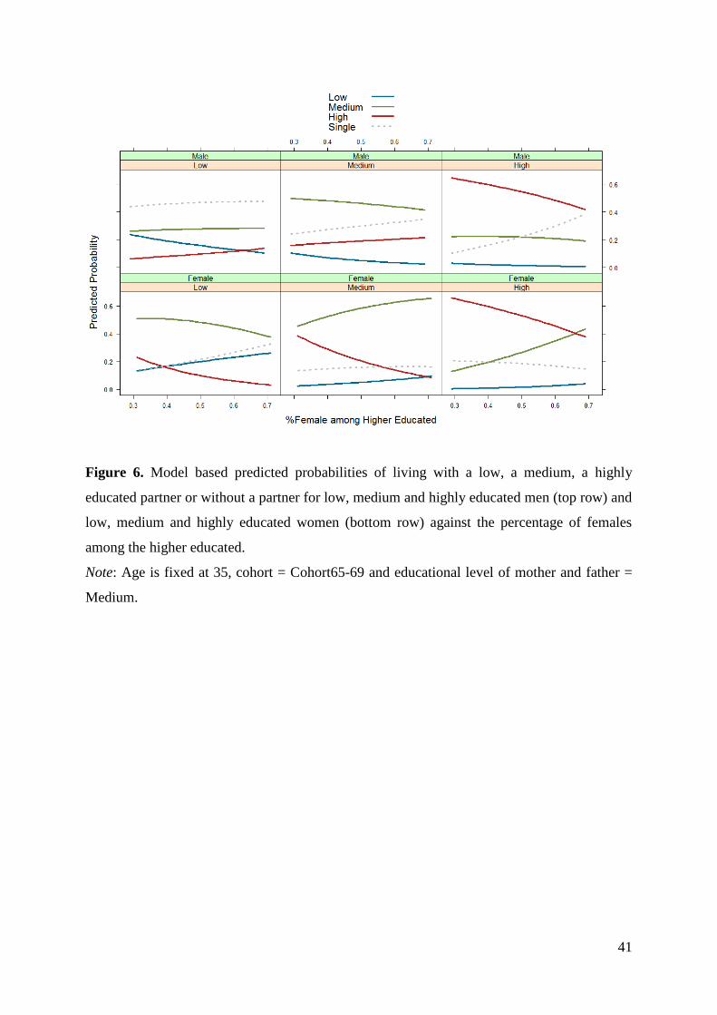
41
Figure 6. Model based predicted probabilities of living with a low, a medium, a highly
educated partner or without a partner for low, medium and highly educated men (top row) and
low, medium and highly educated women (bottom row) against the percentage of females
among the higher educated.
Note: Age is fixed at 35, cohort = Cohort65-69 and educational level of mother and father =
Medium.