The Shift from Classical to Modern Probability: aHistorical Study with Didactical and Epistemological

Reexions

Vinicius Gontijo Lauar

A Thesis

in

The Department

of

Mathematics and Statistics

Presented in Partial Fulllment of the Requirements

for the Degree of

Master of Science (Mathematics) at

Concordia University

Montréal, Québec, Canada

September 2018

© Vinicius Gontijo Lauar, 2018

Concordia UniversitySchool of Graduate Studies

This is to certify that the thesis prepared

By: Vinicius Gontijo Lauar

Entitled: The Shift from Classical to Modern Probability: a Historical Study

with Didactical and Epistemological Reexions

and submitted in partial fulllment of the requirements for the degree of

Master of Science (Mathematics)

complies with the regulations of this University and meets the accepted standards with respect to

originality and quality.

Signed by the Final Examining Committee:

ChairDr. Lea Popovic

ExaminerDr. Alina Stancu

ExaminerDr. Lea Popovic

SupervisorDr. Nadia Hardy

Approved byDr. Cody Hyndman, ChairDepartment of Mathematics and Statistics

2018André Roy, DeanFaculty of Arts and Science

Abstract

The Shift from Classical to Modern Probability: a Historical Study with Didactical andEpistemological Reexions

Vinicius Gontijo Lauar

In this thesis, we describe the historical shift from the classical to the modern denition

of probability. We present the key ideas and insights in that process, from the rst denition

of Bernoulli, to Kolmogorov’s modern foundations discussing some of the limitations of the old

approach and the eorts of many mathematicians to achieve a satisfactory denition of probability.

For our study, we’ve looked, as much as possible, at original sources and provided detailed proofs

of some important results that the authors have written in an abbreviated style.

We then use this historical results to investigate the conceptualization of probability proposed

and fostered by undergraduate and graduate probability textbooks through their theoretical dis-

course and proposed exercises. Our ndings show that, despite textbooks give an axiomatic def-

inition of probability, the main aspects of the modern approach are overshadowed by other con-

tent. Undergraduate books may be stimulating the development of classical probability with many

exercises using proportional reasoning while graduate books concentrate the exercises on other

mathematical contents such as measure and set theory without necessarily proposing a reection

on the modern conceptualization of probability.

iii

Acknowledgments

It is true that I put a massive amount of eort to write this thesis, but at the same time, notrecognizing all the people that supported me during this period would be a huge unrighteousness.

• I will start by my supervisor, Dr. Nadia Hardy, who has not only guided me throughout theconstruction of this thesis but also gave me support, since my beginning at Concordia.

• Many thanks to two special professors who were a great source of inspiration: Dr. GeorgeanaBobos-Kristof, for showing how amazing and important the didactical reexions are and Dr.Anna Sierpinska, for her insightful suggestions and comments.

• I must recognize my friend Nixie for proof reading it from the 1st to the last page and alsofor her incentive and words of encouragement. Thanks to my friends for sharing learn-ing experiences through the courses, in special, John Mark, Nixie, Magloire, Antoine andMandana.

• I also want to express my recognition to the students who let me interview them through1h each just a couple of days before their nal exams.

• Thanks to a special friend, Alexander Motta, who helped me to keep on track from thebeginning to the end of this period.

• I want to thank my mom, Silvia, for spending this last month here, doing nothing, but helpingwith the kids and everything else she could. She made life less harsh and much softer.

• I want to thank my three little ones, Bernardo, Cecilia and Alice (yes, it is hard, but possibleto write a thesis having three kids!). Thanks for understanding all the moments when I hadto be absent to do "this work", and also for using all their means to take me out of work toplay hide and seek.

• Finally, I want to thank my beloved Nalu, for being with me through all this time, giving mesupport, cheering for my success and making me strong to always go on.

iv

Contents

Abstract iii

Acknowledgments iv

List of Figures ix

List of Tables x

1 Introduction 1

1.1 The scope of the thesis . . . . . . . . . . . . . . . . . . . . . . . . . . . . . . . . . 1

1.2 Context and originality of our study . . . . . . . . . . . . . . . . . . . . . . . . . . 3

1.3 The outline of the thesis . . . . . . . . . . . . . . . . . . . . . . . . . . . . . . . . 4

2 Literature Review 6

2.1 Introduction . . . . . . . . . . . . . . . . . . . . . . . . . . . . . . . . . . . . . . . 6

2.2 What are epistemological obstacles? . . . . . . . . . . . . . . . . . . . . . . . . . . 7

2.2.1 The role of non-routine tasks in facing epistemological obstacles . . . . . 8

2.3 Examples of epistemological obstacles in probability . . . . . . . . . . . . . . . . . 9

2.3.1 The obstacle of determinism . . . . . . . . . . . . . . . . . . . . . . . . . . 10

2.3.2 The obstacle of equiprobability . . . . . . . . . . . . . . . . . . . . . . . . 10

2.3.3 The obstacle of proportionality or illusion of linearity . . . . . . . . . . . 12

2.4 Examples of diculties in learning probability . . . . . . . . . . . . . . . . . . . . 14

2.5 Closing remarks . . . . . . . . . . . . . . . . . . . . . . . . . . . . . . . . . . . . . 19

3 A pilot study into graduate students’ misconceptions in probability 21

3.1 Introduction . . . . . . . . . . . . . . . . . . . . . . . . . . . . . . . . . . . . . . . 21

v

3.2 Overview of the pilot study . . . . . . . . . . . . . . . . . . . . . . . . . . . . . . . 22

3.2.1 Part A – Questions on some properties of probability . . . . . . . . . . . . 24

3.2.2 Part B – Questions on countable innite sample spaces . . . . . . . . . . . 25

3.3 Methods of data analysis . . . . . . . . . . . . . . . . . . . . . . . . . . . . . . . . 28

3.4 Results . . . . . . . . . . . . . . . . . . . . . . . . . . . . . . . . . . . . . . . . . . 28

3.5 Discussion . . . . . . . . . . . . . . . . . . . . . . . . . . . . . . . . . . . . . . . . 39

3.6 Final remarks . . . . . . . . . . . . . . . . . . . . . . . . . . . . . . . . . . . . . . 40

4 Classical Probability: The Origins, Its Limitations and the Path to the Modern

Approach 41

4.1 Introduction . . . . . . . . . . . . . . . . . . . . . . . . . . . . . . . . . . . . . . . 41

4.2 Probability before 1900 . . . . . . . . . . . . . . . . . . . . . . . . . . . . . . . . . 44

4.2.1 The origins of probability . . . . . . . . . . . . . . . . . . . . . . . . . . . 44

4.2.2 Bernoulli’s Ars Conjectandi and the denition of probability . . . . . . . . 45

4.2.3 Bernoulli’s law of large numbers . . . . . . . . . . . . . . . . . . . . . . . 47

4.2.4 De Moivre’s work - The Doctrine of Chances . . . . . . . . . . . . . . . . . 55

4.2.5 Bayes’ contribution . . . . . . . . . . . . . . . . . . . . . . . . . . . . . . . 56

4.2.6 Paradoxes in classic probability . . . . . . . . . . . . . . . . . . . . . . . . 57

4.3 The development of measure theory . . . . . . . . . . . . . . . . . . . . . . . . . . 60

4.3.1 Gyldén’s continued fractions . . . . . . . . . . . . . . . . . . . . . . . . . 61

4.3.2 Jordan’s inner and outer content . . . . . . . . . . . . . . . . . . . . . . . 62

4.3.3 Borel and the birth of measure theory . . . . . . . . . . . . . . . . . . . . 63

4.3.4 Lebesgue’s measure and integration . . . . . . . . . . . . . . . . . . . . . 68

4.3.5 Radon’s generalization of Lebesgue’s integral . . . . . . . . . . . . . . . . 72

4.3.6 Carathéodory’s axioms for measure theory . . . . . . . . . . . . . . . . . 74

4.3.7 Fréchet’s integral on non-Euclidian spaces . . . . . . . . . . . . . . . . . . 76

4.3.8 The Radon-Nikodym theorem . . . . . . . . . . . . . . . . . . . . . . . . . 77

4.4 The search for the axioms and early connections between probability and measure

theory. . . . . . . . . . . . . . . . . . . . . . . . . . . . . . . . . . . . . . . . . . . 79

4.4.1 The connection of measure and probability and the call for the axioms . . 79

4.4.2 Borel’s denumerable probability . . . . . . . . . . . . . . . . . . . . . . . . 80

vi

4.4.3 The rst attempts at axiomatization . . . . . . . . . . . . . . . . . . . . . 85

4.4.4 The proofs of the strong law of large numbers . . . . . . . . . . . . . . . . 89

5 Kolmogorov’s foundation of probability 92

5.1 Introduction . . . . . . . . . . . . . . . . . . . . . . . . . . . . . . . . . . . . . . . 92

5.2 Kolmogorov’s axioms of probability . . . . . . . . . . . . . . . . . . . . . . . . . . 94

5.2.1 Elementary theory of probability . . . . . . . . . . . . . . . . . . . . . . . 94

5.2.2 Innite probability elds . . . . . . . . . . . . . . . . . . . . . . . . . . . . 95

5.3 Denitions in modern probability . . . . . . . . . . . . . . . . . . . . . . . . . . . 98

5.3.1 Probability functions and random variables . . . . . . . . . . . . . . . . . 98

5.3.2 Mathematical expectation . . . . . . . . . . . . . . . . . . . . . . . . . . . 100

5.3.3 Conditional probability . . . . . . . . . . . . . . . . . . . . . . . . . . . . . 101

5.3.4 Expectation conditional to a σ-algebra . . . . . . . . . . . . . . . . . . . . 105

5.4 The great circle paradox . . . . . . . . . . . . . . . . . . . . . . . . . . . . . . . . 107

5.4.1 Closing remarks from the great circle paradox . . . . . . . . . . . . . . . . 110

6 Book Analysis 112

6.1 Introduction . . . . . . . . . . . . . . . . . . . . . . . . . . . . . . . . . . . . . . . 112

6.2 Methodology . . . . . . . . . . . . . . . . . . . . . . . . . . . . . . . . . . . . . . . 113

6.2.1 The book selection . . . . . . . . . . . . . . . . . . . . . . . . . . . . . . . 113

6.2.2 The characterization of the books . . . . . . . . . . . . . . . . . . . . . . . 113

6.2.3 Analysis of the set of exercises . . . . . . . . . . . . . . . . . . . . . . . . 114

6.3 Book analysis . . . . . . . . . . . . . . . . . . . . . . . . . . . . . . . . . . . . . . 115

6.3.1 Book 1: Wackerly, D. D. ; Mendenhall, W. and Scheaer, R. L. Mathematical

Statistics with Applications [68]. . . . . . . . . . . . . . . . . . . . . . . . 115

6.3.2 Discussion . . . . . . . . . . . . . . . . . . . . . . . . . . . . . . . . . . . . 118

6.3.3 Book 2: Ross, S. A rst course in probability [52]. . . . . . . . . . . . . . . 120

6.3.4 Discussion . . . . . . . . . . . . . . . . . . . . . . . . . . . . . . . . . . . . 124

6.3.5 Book 3: Grimmet, G. R. and Stirzaker, D. R. Probability and Random Pro-

cesses [27]. . . . . . . . . . . . . . . . . . . . . . . . . . . . . . . . . . . . 126

6.3.6 Discussion . . . . . . . . . . . . . . . . . . . . . . . . . . . . . . . . . . . . 128

6.3.7 Book 4: Shiryaev, Probability 1 [59]. . . . . . . . . . . . . . . . . . . . . . 129

vii

6.3.8 Discussion . . . . . . . . . . . . . . . . . . . . . . . . . . . . . . . . . . . . 133

6.3.9 Book 5: Durrett, R. Probability: Theory and Examples [22]. . . . . . . . . 133

6.3.10 Discussion . . . . . . . . . . . . . . . . . . . . . . . . . . . . . . . . . . . . 135

6.4 Final remarks . . . . . . . . . . . . . . . . . . . . . . . . . . . . . . . . . . . . . . 136

7 Final Remarks 139

7.1 Remarks on the history and foundation of probability . . . . . . . . . . . . . . . . 139

7.2 Remarks on the didactical implications . . . . . . . . . . . . . . . . . . . . . . . . 142

7.3 Originality, limitations and future research . . . . . . . . . . . . . . . . . . . . . . 143

Bibliography 145

viii

List of Figures

Figure 4.1 Chord paradox - [1] (p. 4). . . . . . . . . . . . . . . . . . . . . . . . . . . . 58

Figure 4.2 Buon’s needle paradox - [1] (p. 6). . . . . . . . . . . . . . . . . . . . . . . 59

Figure 4.3 Jordan’s partition - [34] (p. 276). . . . . . . . . . . . . . . . . . . . . . . . . 63

Figure 4.4 The convex curve C - [33] (p. 98). . . . . . . . . . . . . . . . . . . . . . . . 64

Figure 4.5 Connection of P and Q - [33] (p. 100). . . . . . . . . . . . . . . . . . . . . . 65

Figure 4.6 Khintchin’s bounds - [46] (p. 260). . . . . . . . . . . . . . . . . . . . . . . . 91

Figure 5.1 Kolmogorov’s axioms I to V - [39] (p. 2). . . . . . . . . . . . . . . . . . . . 94

Figure 5.2 Kolmogorov’s axiom VI - [39] (p. 14). . . . . . . . . . . . . . . . . . . . . . 95

Figure 5.3 The great circle paradox - [29] (p. 2612 and 2614). . . . . . . . . . . . . . . 108

Figure 5.4 Parametrization of the sphere - [1] (p. 83). . . . . . . . . . . . . . . . . . . 109

Figure 6.1 Denition of probability - [68] (p. 30). . . . . . . . . . . . . . . . . . . . . . 117

Figure 6.2 Venn diagram - Exercises from [68]. . . . . . . . . . . . . . . . . . . . . . . 119

Figure 6.3 Denition of probability - [52] (p. 27) . . . . . . . . . . . . . . . . . . . . . 121

Figure 6.4 Example 6a - [52] (p. 46). . . . . . . . . . . . . . . . . . . . . . . . . . . . . 123

Figure 6.5 Continuation of example 6a - [52] (p. 46). . . . . . . . . . . . . . . . . . . . 123

Figure 6.6 Venn diagram - Exercises from [52]. . . . . . . . . . . . . . . . . . . . . . . 124

Figure 6.7 Denition of probability - [27] (p. 5). . . . . . . . . . . . . . . . . . . . . . 127

Figure 6.8 Lemma - [27] (p. 6). . . . . . . . . . . . . . . . . . . . . . . . . . . . . . . . 127

Figure 6.9 Venn diagram - Exercises from [27]. . . . . . . . . . . . . . . . . . . . . . . 128

Figure 6.10 Assigning probability to innite sets - [59] (p. 160). . . . . . . . . . . . . . 131

Figure 6.11 Venn diagram - Exercises from [59]. . . . . . . . . . . . . . . . . . . . . . . 132

Figure 6.12 Denition of probability space - [22] (p. 1) . . . . . . . . . . . . . . . . . . 134

Figure 6.13 Venn diagram - Exercises from [22] . . . . . . . . . . . . . . . . . . . . . . 135

ix

List of Tables

Table 3.1 Questions A1 . . . . . . . . . . . . . . . . . . . . . . . . . . . . . . . . . . . 29

Table 3.2 Questions A2 to A5 . . . . . . . . . . . . . . . . . . . . . . . . . . . . . . . . 30

Table 3.3 Warm up question B.1 . . . . . . . . . . . . . . . . . . . . . . . . . . . . . . 31

Table 3.4 Warm up question B.2 . . . . . . . . . . . . . . . . . . . . . . . . . . . . . . 32

Table 3.5 Question B1 . . . . . . . . . . . . . . . . . . . . . . . . . . . . . . . . . . . . 32

Table 3.6 Question B2 . . . . . . . . . . . . . . . . . . . . . . . . . . . . . . . . . . . . 33

Table 3.7 Question B3 . . . . . . . . . . . . . . . . . . . . . . . . . . . . . . . . . . . . 33

Table 3.8 Question B4 . . . . . . . . . . . . . . . . . . . . . . . . . . . . . . . . . . . . 34

Table 3.9 Question B5 . . . . . . . . . . . . . . . . . . . . . . . . . . . . . . . . . . . . 35

Table 3.10 Question B6 . . . . . . . . . . . . . . . . . . . . . . . . . . . . . . . . . . . . 36

Table 3.11 Question B7 . . . . . . . . . . . . . . . . . . . . . . . . . . . . . . . . . . . . 37

Table 3.12 Question B8 . . . . . . . . . . . . . . . . . . . . . . . . . . . . . . . . . . . . 38

x

Chapter 1

Introduction

1.1 The scope of the thesis

This thesis was catalyzed by two curiosities we had in mind: if probability has been studied for

many centuries, i) why do its foundations date from 1933? and ii) why is it associated to measure

theory1?

The foundations of the modern theory of probability were laid out by the Russian mathemati-

cian Andreï Nikolaïevitch Kolmogorov in his book: Foudations of the Theory of Probability2 in

1933. At the beginning of the 18th century, Jacques Bernoulli and Abraham de Moivre published

the rst works with the denition of probability that became, two centuries later, following the

work of Kolmogorov, a generalized and abstract theory of probability. Although Cardano, Mont-

mort, Pascal and others had already made advances with the calculations of the number of possible

outcomes for two or three die throws and the addition and multiplication rules, the outstanding

breakthrough of Bernoulli and de Moivre, in relation to their predecessors, is that they were the

rst to dene probability and expectation with a greater level of generality. Bernoulli discovered

and proved the rst version of a very important convergence theorem, the law of large numbers,

and de Moivre was aware of the generality of the results that others were applying to specic

problems.

The classical denition of probability by Bernoulli and de Moivre remained essentially the1Measure theory started with the works of Borel and Lebesgue in the transition from the 19th to the 20th century.2The origial version was written in German and is called "Grundbegrie der Wahrscheinlichkeitsrechnung"

1

same throughout the 18th and 19th centuries. Yet, as science evolved through time, contradictions

and paradoxical results began to reveal the limitations of classical probability, requiring a new and

precise denition of probability and other related concepts. It was not until the development of

measure theory and the Lebesgue integral beyond Euclidean spaces that the modern and axiomatic

denition of probability in its complete and abstract form was developed and probability was raised

from a set of tools in applied mathematics to a branch on its own.

Kolmogorov’s modern denition of probability may be seen by an unaware and naive per-

son as a fully-born concept. A sudden, brilliant and original idea that triumphed over chaos and

confusion. Even if Kolmogorov’s book contains some original contributions, it is also seen as a

work of synthesis [56]. History of mathematics cannot be limited to the formal results presented

in the standard textbooks. The imprecise and contradictory developments also play an important

role in the advances of science [19], [17]. The advances in mathematics are almost always built

on the work of people who contribute little by little over hundreds of years. Eventually, someone

is able to distinguish the valuable ideas of their predecessors among the myriad of statements to

t existing knowledge into a new approach. This was exactly the case of Kolmogorov, because

many results from measure theory3, set theory4, probability5 and even unsuccessful attempts to

an axiomatization,6 were relevant to his foundation of modern probability. The famous statement

attributed to Newton: "If I have seen further it is by standing on the shoulders of Giants" also applies

to Kolmogorov.

Given the above context, we can state the rst problem this thesis sought to answer: If prob-

ability has been present in mathematics for many centuries, why the advent of measure theory

was a turning point in the denition and conceptualization of probability. More specically, why

did probability need measure theory as its basis to be considered an autonomous branch of math-

ematics?

By understanding this evolution from classical to modern probability and the importance of

Kolmogorov’s axiomatization up to the point that probability was raised to an autonomous branch3Example of authors: Borel, Lebesgue, Carathéodory, Fréchet, Radon and Nikodyn4Example of authors: Cantor and Hausdor5Example of authors: Borel, Cantelli, Lévy, Slutsky and Steinhaus6Example of authors: Laemmel, Hilbert, Broggi, Lomnicki, Bernstein, von Mises and Slutsky

2

of mathematics, a second research question that attaches a didactical value to this thesis emerged:

Considering the classical and the modern approaches to probability, which one of them are pri-

marily advanced by undergraduate and graduate textbooks?

The investigation of this problem started in a literature review on epistemological obstacles

in mathematics and in probability. Due to the near absence of studies considering probability at

the post-secondary level, we’ve done a pilot test. We’ve interviewed four graduate students to

investigate whether their conceptualization of probability is closer to a classical or to a modern

approach. We have found a persistence of two epistemological obstacles7. The rst one is the ob-

stacle of equiprobability, that is, a tendency to believe that elementary events are equiprobable (i.e.,

uniform) by nature. The second is the proportionality obstacle or illusion of linearity, that is, the

epistemological obstacle of using proportional reasoning in situations where it is not appropriate.

In probability the illusion of linearity comes from the habit of identifying probability as a ratio of

favourable over possible cases.

Once the obstacles of equiprobability and proportionality were found in the pilot test, we’ve

looked at some undergratuate and graduate textbooks used in the four universities in Montreal

with the goal of identifying how those books introduce the denition of probability and how they

help students develop, though the exercises and examples, a modern or a classical view of the

domain.

1.2 Context and originality of our study

In the previous section we’ve presented the context regarding the shift in probability from a

classical approach to a modern theory developed by Kolmogorov. In this thesis, this evolution of

probability is detailed with some relevant mathematical results developed in full, based on original

sources8, to evidence some mathematical ideas or to present in details some proofs. The goal is to

display great ideas from each author’s contribution to the foundations of modern probability.

We tried, as much as possible, to bring attention to the motivation for the discoveries and also

to present some ideas that were unsuccessful to show that the development of the theory didn’t7See chapter 2 for more details.8When the original source was available in English or French.

3

follow a straightforward path.

The didactical contribution is also original, because there is a scarcity of research in post-

secondary level of probability learning. While the proportionality obstacle has been identied as

a common epistemological obstacle in high school, we have identied its persistence in graduate

level studies. The obstacle of equiprobability has been researched in dierent educational levels,

but here we apply it along with the illusion of linearity to the conceptualization of probability. Fur-

thermore, we’ve also done an investigation into the approach to probability taken by the books

used most commonly by Montreal universities, as well as an anaylysis of the proposed exercises,

seeking to nd some of the potential sources for the proportionality and equiprobability obsta-

cles. These didactical reections appeal to readers interested in the teaching of probability at the

undergraduate and graduate levels.

1.3 The outline of the thesis

In the second chapter we present a literature review on three important topics for this thesis:

i) epistemological obstacles in mathematics education, ii) examples of epistemological obstacles in

probability and iii) misconceptions in probability.

The third chapter presents a pilot study with graduate students aimed at discovering whether

these students conceptualize probability in a classical or in a modern sense, or using a mix of both.

We’ve found that the epistemological obstacle of identifying probability as a ratio of favourable

over possible cases in situations where it doesn’t apply is persistent and we associate it to the

obstacles of proportionality and equiprobability.

The fourth chapter answers by itself one of the main goals of this thesis. It explain why prob-

ability became attached to measure theory at the beginning of the 20th century. More specically,

it explains why probability needed measure theory as its basis to be considered an autonomous

branch of mathematics. The chapter presents the origins of probability and its development, in-

cluding the rst denition of this concept and the contributions from Bernoulli and de Moivre. It

also discusses the evolution of measure theory with focus on the results that were important to

the development of modern probability, and the association of both disciplines since its foundation

4

with Borel and Lebesgue. We also expose the need to develop a general and abstract set of axioms

for probability and the rst attempts at an axiomatization. At the end of the chapter, we discuss

Borel’s denumerable probability, more specically the use of countable additivity and the strong

law of large numbers, two essential results to the foundation of the axioms.

In the fth chapter we discuss the axiomatic denition of probability in Kolmogorov’s book for

nite and innite spaces and the change in the concept of conditional probability to illustrate how

this step into modern probability established a fertile ground to rigorous and general denitions

of terms that were loosely used in the classical era. As an illustration, there is an example that

leads to a paradox in classical probability that was resolved by Kolmogorov’s new approach using

conditional probability.

The sixth chapter analyzes some of the most commonly used probability textbooks in the

four universities in Montreal. The goal is to analyze how those books introduce the denition

of probability and if their proposed exercise sets require students thinking about Kolmogorov’s

innovation or if they stimulate the idea of probability as a ratio of favourable over possible cases

– even perhaps reinforcing the epistemological obstacles of equiprobability and proportionality.

The thesis nishes with the seventh chapter, where we draw a summary of the ndings and

discuss some recommendations for the teaching of probability.

5

Chapter 2

Literature Review

2.1 Introduction

This literature review is focused on epistemological obstacles and other sources of diculties

in learning probability. The focus is the concept of epistemological obstacles in learning math-

ematics, some examples of epistemological obstacles in probability and a brief survey of some

diculties in learning probability. This literature review doesn’t concern all the diculties in

learning probability and doesn’t intend to cover the whole subject of epistemological obstacles,

but rather to present the denition of the term and exemplify how it applies to probability, besides

showing some common diculties in probability that have been studied.

The literature on epistemological obstacles and diculties in learning probability is very ex-

tensive, however, we didn’t nd any publications related to the teaching and learning of probability

at the post-secondary level, and in particular, no publications related to the teaching and learning

of the axiomatic denition of probability. This is exactly the gap that this thesis aims to contribute

to ll up.

This review is presented in four sections. After this introduction, the second section discusses

texts that introduce the concept of epistemological obstacles in mathematics. The third section

applies this concept to probability and gives three examples. The fourth section presents some

of the research in diculties in learning probability and the chapter nishes with some closing

remarks.

6

2.2 What are epistemological obstacles?

Brousseau [15] and [16] was the rst to transpose the concept of epistemological obstacle to the

didactics of mathematics by highlighting the change that the theory of epistemological obstacles

proposes in the status of the error : L’erreur n’est pas seulement l’eet de l’ignorance, de l’incertitude,

[...] mais l’eet d’une connaissance antérieure, qui avait son intérêt, ses succès, mais qui, maintenant,

se révèle fausse, ou simplement inadaptée" [16] (p. 104).

The term epistemological obstacle was proposed by Bachelard [3] in his studies of the history

and philosophy of science. The concept was rst applied to mathematics education by Brousseau

[15], [16]. Among the learning obstacles, Brousseau distinguishes three categories: i) ontogenic

obstacles, genetic and psychological obstacles developed as a result of the cognitive and personal

development of the student, ii) didactic obstacles, which come from the didactic choices and iii)

the epistemological obstacles, that happen because of the nature of the mathematical concepts

themselves and from which there is no escape due to the fact that they play a constitutive role in

the construction of knowledge.

In this review, we will focus on epistemological obstacles, because we are interested in the

obstacles related to the nature of the mathematical concepts, such as probability, random vari-

able and mathematical expectation. Sierpinska [62] dened epistemological obstacles as "ways of

understanding based on some unconscious, culturally acquired schemes of thought and unquestioned

beliefs about the nature of mathematics and fundamental categories such as number, space, cause,

chance, innity,... inadequate with respect to the present day theory" (p. xi).

As an example, the daily life usage of the word limit as a barrier that should not be crossed

may be an epistemological obstacle that the student needs to confront when studying the limit of a

function. Similarly, the vast experience acquired with linearity from early school years and many

daily life situations often leads to an inclination to use linear models or a proportional reasoning

where these should not be applied. As an example, many people think that getting 2 heads out of

three coin tosses is equally likely to 6 heads in nine coin tosses.

Sierpinska [61] and [62], concerned with mathematical learning, describes the concept of un-

derstanding as an act involved in a process of interpretation. This interpretation process is the

7

development of a dialectic between more and more elaborate guesses and validations of these

guesses. With this interpretation of understanding, she describes the relationship between episte-

mological obstacles and understanding in mathematics.

At a certain moment, typically when facing a new problem, we discover that our current math-

ematical knowledge is not accurate (e.g., understanding limit as a barrier may be accurate in the

context of nding the limits of rational functions - horizontal asymptotes - but is no longer accu-

rate when studying limits of functions that oscillate about their limit). This is when we become

aware of an epistemological obstacle. So we understand something and we start knowing in a

new way, which might turn into another epistemological obstacle in another situation. The act

of understanding is the act of overcoming an epistemological obstacle. Sierpinska points out that

some acts of understanding may turn out as acquiring new epistemological obstacles.

In many cases overcoming an epistemological obstacle and understanding are just two ways of

speaking about the same thing. Epistemological obstacles look backwards, focusing the attention

on what was wrong, insucient, in our ways of knowing. Understanding looks forward to the

new ways of knowing. We do not know what is really going on in the head of a student at the

crucial moment but if we take the perspective of his or her past knowledge we see him or her

overcoming an obstacle, and if we take the perspective of the future knowledge, we see him or her

understanding.

2.2.1 The role of non-routine tasks in facing epistemological obstacles

As Sierpinska [62] explains, the successive acts of understandings are obtained through facing

rather than avoiding epistemological obstacles. Hardy [32] and Schoenfeld [55], among others,

discuss the role of tasks, typically given to students in hiding epistemological obstacles. Hardy

studied how college students learn calculus and more specically, the inuence of routine tasks

and the institutional environment in their way of thinking and solving problems. Most of the tasks

that students face (thus called routine tasks) when they learn limits are of the type nd the limit of

a continuous function or of a function whose required limit becomes trivial after some common

algebraic operations.

To Schoenfeld, each group of routine tasks adds a mathematical tool kit to the student and the

8

sum of these techniques reects the corpus of mathematics that the student should learn. This

environment of blocs of routine tasks enhances the view of mathematics as a canon, instead of a

science. As consequences of routine tasks: i) students are not expected to gure out the methods

by themselves and acquire a passive behaviour because they think that the only valid method to

solve a given set of problems is the one provided by the instructor; ii) it also makes students think

that one should have a ready method for the solution of the mathematical problems and iii) gener-

ates an automatic behaviour towards tasks, as the students read the rst few words of a problem,

they already know what will be asked and what is the method that should be used. Practices based

on routine tasks and weak theoretical content do not challenge students’ modes of thinking, in

particular, they don’t force students to face epistemological obstacles. Both authors, show and il-

lustrate how non-routine tasks, carefully crafted to reveal misconceptions, make students confront

and overcome them, thus advancing their learning.

For students to gain a sense of the mathematical enterprise, their experience with mathemat-

ics must be consistent with the way mathematics is done. The articiality of the examples moves

the corpus of exercises from the realm of the practical and plausible to the realm of the articial,

which makes students give up to make sense of mathematics. Sierpniska, Schoenfeld and others

emphasize that the focus should be changed from content to modes of thinking. Handling new

and unfamiliar tasks, possibly using unknown methods should be at the heart of problem solving.

While routine tasks may foster a passive behaviour, non-routine tasks, if well elaborated, can help

students to confront their epistemological obstacles and promote successive acts of understand-

ings.

2.3 Examples of epistemological obstacles in probability

In the previous section we introduced the term epistemological obstacle in mathematics. In this

section we present some examples of those obstacles in probability. As will be shown in chapter

ve, those obstacles played a signicant role in the evolution of the theory of probability as they

consisted of granted beliefs about chance that lead to theoretical inconsistencies and diculties in

solving problems.

9

2.3.1 The obstacle of determinism

Borovcnik and Kapadia [14] describe probability from a historical an philosophical perspective.

According to them, since the roman empire, when Christianity became the only allowed religion

under Theodosius (around 380 A.D.), games of chance, which were a great incentive to the devel-

opment of probability, lost prestige as everything that happens is determined by the will of god.

The dominant idea was that randomness comes from man’s ignorance instead of the nature of

the events. This belief that any phenomena is deterministic and could be predicted with absolute

certainty if we were aware of all the variables of inuence is what we call the obstacle of determin-

ism. This epistemological obstacle has existed from ancient times, passing through the classical

era of probability and is still present in some people’s mind today. In the original texts of Bernoulli

[7], DeMoivre [21] and Laplace [41], we can see that, as it was common during their time, they

considered the world to be deterministic. The omnipotent and omniscient god determines every

event, usually by causal laws, leaving no space to chance. Hence probability, was a tool used to

make decision due to our ignorance of all the factors that determine an event [30]. Von Plato [67]

shows the reluctance in accepting randomness in the essence of matter in the early 20th century.

2.3.2 The obstacle of equiprobability

The obstacle of equiprobability came from the idea that elementary events are equiprobable.

Laplace created the principle of indierence, where he attributed equal probability to all events

when we have no reason to suspect that any one of the cases is more likely to occur than the

others. This principle was adopted in his denition of probability: "La théorie des hasards consiste

à réduire tous les événements du même genre, à un certain nombre des cas également possibles, c’est-

à-dire, tels que nous soyons également indécis sur leur existence; et à déterminer le nombre de cas

favorables à l’événement dont on cherche la probabilité. Le rapport de ce nombre à celui de tous les

cas possibles, est la mesure de cette probabilité qui n’est ainsi qu’une fraction dont le numérateur est le

nombre des cas favorables, et dont le dénominateur est le nombre de tous les cas possibles" [41] (p. iv).

The principle of indierence and the denition of probability as a ratio of equally likely cases have

shown its limitations in probability and that are one of the main motivations for the foundations

10

of modern probability, as we describe in chapter four.

The obstacle of equiprobability is introduced in the literature by [45]. Gauvrit and Morsanyi

[25] describe it as the tendency of using a uniform distribution for events where it is not appro-

priate. They argue that many times, although not always, this obstacle is present because some

experiments consist in analyzing a non-uniform random variable that was originated by the com-

bination of two or more uniform random variables. Among many examples in modern literature

involving this obstacle, we will present the two children problem and the Monty Hall problem.

In the two children problem, consider a person has two kids. If at least one of them is a boy,

what is the probability that both children are boys? The correct answer is easily found by setting

equally likely ordered pairs: (girl, boy), (boy, girl) and (boy, boy), so the correct answer would be

1/3. However, when unordered pairs are considered, girl, boy or boy, boy, they are not equally

likely. Their probabilities are, respectivelly, 2/3 and 1/3, but many people consider that they share

the same probability of the ordered pairs, so give the incorrect answer of 0.5.

Another example of the equiprobability obstacle is the very well known Monty Hall problem.

In a game, a participant should choose one out of three doors, say A, B or C. Behind one of them,

there is a prize and behind the others, there isn’t. The participant picks a door, say C. After that,

one door without the prize is opened (say B) and is shown to the participant. Then it is asked to

the participant if she/he would prefer to stay with door C or to change to door A. Thinking that

doors A and C have the same probability of having the prize after door B opened, is an incorrect

reasoning given by the obstacle of equiprobability. At the rst moment, all three doors have the

same probability of having the prize. Once the participant has picked door C, the probability that

the prize is in the set A ∪ B is 2/3. When presenter of the game opens door B, it is not done at

random, because she/he knows that the prize is not in door B. That means that the door A has

probability 2/3 of having the prize while door C has probability 1/3. So the best strategy would be

to change doors.

The interpretation of equiprobability of elementary events is problematic, specially when the

probability space, Ω, is innite (countable or not). In a countable innite space, by countably

additivity, P (Ω) must be either 0, if each elementary event has probability zero, or innity, if to

each elementary event would be assigned one constant positive probability.

11

In an uncountable probability space, like the interval [0, 1], let’s consider any sub-interval

(a, b) ⊂ [0, 1]. If we set Px ∈ (a, b) = b− a, that is, the probability of x be in the sub-interval

(a, b) is the length of that interval, then we say that x is uniformly chosen at random. Intuition

may suggest that if we provide two descriptions of one set of elementary outcomes that can be

bijectively related to each other, then if in one of them the elementary outcomes are equiprobable,

the same should be true under the other description. However, this epistemological obstacle leads

to a paradox found in Poincaré [51] and in Borel [12]. Let y = x2. Can x and y be considered uni-

formly chosen at random? For any x ∈ [0, 1], we nd a corresponding y ∈ [0, 1]. The probability

that x ∈ [0, 1/2] is 1/2, and the probability that y ∈ [0, 1/4] is 1/4, but both probabilities should

be the same, according to the bijection established between the descriptions of the elements of the

interval [0, 1].

2.3.3 The obstacle of proportionality or illusion of linearity

The proportionality obstacle or illusion of linearity is “...the strong tendency to apply linear

or proportional models anywhere, even in situations where they are not applicable” [65] (p. 113).

The illusion of linearity is classied as an epistemological obstacle because it has implications in

the historical development of probability, but it is also considered a didactic obstacle due to the

extensive attention given to proportional reasoning in mathematics education.

The illusion of linearity takes place because the notions of proportion and chance are cogni-

tively and intuitively very closely related to each other. The over-reliance in proportions cause

errors in probability thinking. The classical denition of probability, as we will discuss in chap-

ter four, is given by a fraction or proportion of favourable over possible cases. Thus, comparing

probabilities is a comparison of two fractions, so proportional reasoning is considered to be a basic

tool in this domain since the rst notions of chance in the 16th and 17th centuries even before the

classical denition.

The obstacle of proportionality may be found in terms of distance between two probability

values, specially when we consider events of probability 0 or probability 1. Let’s take a non-

symmetric coin, with probability of heads p 6= 0.5. We toss the coin repeatedly many times

and register the relative frequency of heads. The law of large numbers tells us that the dierence

12

between the relative frequency of heads in that sequence and the value 0.5 could be made arbitrarily

small by making p arbitrarily close to 0.5. This situation doesn’t apply when we consider a coin

with probability of heads arbitrarily close (but not equal) to 0 and another coin with probability

of heads equal to zero.

To see that, let’s take two biased coins, the rst with probability of showing heads of 0.0001

and the second probability 0.00001. Even if the dierence |0.0001−0.00001| is very small, the ratio

0.001/0.0001 makes the expected number of heads in the rst n outcomes 10 times greater in the

rst sequence than in the second one. A coin αwith any arbitrarily small, but positive, probability

of heads produces innitely dierent sequences than a coin β with probability of heads equal

to zero. This happens because the coin α should produce sequences of outcomes with innitely

many heads and the coin β should show a nite number of it, which congures a very dierent

behaviour.

The Italian mathematician Cardano (1501–1576) made considerable gains in gambling because

of his knowledge of chance1. He correctly reasoned that the probability of getting double ones in a

die throw is 1/36, but felt into the obstacle of proportionality when he thought that he had to throw

the dice 18 times to have a probability of 1/2 to get a double ones at least once (18× 1/36 = 1/2).

De Méré (1607-1684), a notorious gambler, knew by experience that it was advantageous to

bet on at least 1 six in 4 rolls of a die. Using a proportional reasoning, he thought that it was

also advantageous to bet on at least 1 double-six in 24 rolls of two fair dice (4/6 = 24/36). It was

Pascal who explained him that the probability of 1 six in 4 trials equals 1 − (5/6)4 = 0.52, but 1

double-six in 24 rolls of two dice is 1− (35/36)24 = 0.49.

The illusion of linearity is also reiforced by didactical choices, which makes it a didactical

obstacle. In this sense, one of the causes of the illusion of linearity is the extensive attention given

to proportional reasoning in mathematics education. As the proportional (or linear) model is a

key concept in primary and secondary education with a very wide applicability, students get so

familiar with it that they usually stick to a linear approach in situations where it doesn’t apply.

In fact, Piaget and Inhelder [49] believe that understanding proportions and ratios is essential

for children to understand probability. Lamprianou and Afantiti Lamprianou [40] suggest that1In Cardano’s time, the word chance was used to designate probability.

13

comparing fractions is necessary for probabilistic reasoning in children.

Van Doren (and others) [65] presented some situations like in Cardano’s and de Méré’s prob-

lems to 10th and 12th grade students in an empirical experiment. Before instruction, students had

compared events correctly at a qualitative level. Nevertheless, these students erroneously trans-

lated their qualitative reasoning using proportional relationships. The illusion of linearity was

present and persistent, even after instruction.

2.4 Examples of diculties in learning probability

We have presented the notion of epistemological obstacle in mathematics and given some

examples in probability. Now we present a discussion on some sources of diculties in learning

probability reported in the literature. Some of these diculties are epistemological obstacles and

some are not. It’s important to remark that the authors, whose work we discuss below, were not

thinking in terms of epistemological obstacles when they’ve done their research. We don’t intend

to enter in the whelm of ontogenic or didactical obstacles. The purpose here is to present some

research that has been done related to diculties in learning probability and also some teaching

experiences that can illustrate the epistemological obstacles of the previous section. We start with

the text of Shaughnessy [57], which is a vast survey of research on the teaching of probability and

statistics, what he calls the teaching of stochastics.

With the same concern about mathematical thinking as Hardy and Sierpinska have, Shaugh-

nessy suggests that naive heuristics that are used intuitively by learners impede the conceptual

understanding of terms such as sampling, conditional probability and independence (i.e., causal

schemes), decision schema (i.e., outcome approach), and the mean. The main themes investigated

in his paper are the research on judgmental heuristics and biases that lead to misconceptions and

wrong calculations. Learners have diculties in these areas, however, evidence is contradictory

as to whether instruction in stochastics improves performance and decreases misconceptions.

The conclusions emerging from his research are i) probability concepts can and should be

introduced in school at an early age, ii) instruction that is designed to confront misconceptions

should encourage students to test whether their beliefs coincide with those of others, whether they

14

are consistent with their own beliefs about other related things, and whether their beliefs come

from empirical evidence.

Shaughnessy [57] presents a very broad review of what has been done in terms of research

in probability and statistics teaching and learning, more precisely, presenting the misconceptions

and diculties students have in learning stochastics. We will present the ones most relevant to

learning probability theory.

The problem of representativeness: people estimate likelihoods for events based on how

well an outcome represents some aspect of its population. People believe that a sample (or even a

single event) should reect the distribution of the parent population or should mirror the process

by which random events are generated. As an example of the problem of representativeness: in

a sequence of boys and girls of a family with 6 children: the sequence BGGBGB is believed to be

more likely to happen than BBBBGB or BBBGGG. However, the 3 of them are equally probable.

Representativeness heuristic has also been used to explain the “gambler’s fallacy”. After a

run of heads, tails should be more likely to come up. People try to predict the result that was

appearing less often in order to balance the ratio after a small number of trials. Once they have

some information about the distribution, even from small sample sizes, they tend to put too much

faith in that information. Even very small samples are considered to be representative.

The problem of representativeness is related to the obstacle of proportionality, when people

apply a linear reasoning for dierent sample sizes of an experiment, and also to the obstacle of

equiprobability, when people guess the next outcome as the event that will balance the ratio.

The availability problem: the estimation of the likelihood of events are biased by how easy

it is to recall such events. If a situation has happened to person A, this person will actually think

it’s more probable to happen than an objective frequency distribution would tell.

The conjunction fallacy: to rate certain types of conjunctive events more likely to occur

than their parent stem events. The reason for saying that P (A ∩B) > P (A) may come from the

fact that the event B may have a much higher probability than the event A. Also, people may

have a language misunderstanding, when told P (A ∪B), they may understand P (A|B).

Research on conditional probability and independence: One of the most common mis-

conceptions about conditional probability arises when a conditioning event occurs after the event

15

that it conditions.

As an example: an urn has 2 white and 2 black balls in it. Two balls are drawn without re-

placement. What’s the probability that:

1. The second ball is white, given that the rst ball was white? P (W2|W1)

2. The rst ball was white given that the second ball is white? P (W1|W2)

A common confusion is with the rst and the second statements. Many times it’s asked

P (W2|W1) and people usually answerP (W1|W2). Other problems show how diculties in select-

ing the event to be the conditioning event can lead to misconceptions of conditional probabilities.

Example: There are three cards in a bag. One with both sides green, one with both sides blue

and the third one with a blue and a green side. You pull out a card and see that one side is blue.

What is the probability that the other side is also blue?

The typical answer, 0.5, assumes a uniform probability, by considering the cards blue-blue and

blue-green equiprobable. The correct answer is dierent, because the 3 sides of the two possible

cards are blue, and the blue-blue card has two blue sides, the probability is actually 2/3. This

problem is another example of the equiprobability obstacle because we can see a search for a

uniform probability where it doesn’t apply.

In general, students often confuse P (A|B) with P (B|A). This happens because:

• Students may have diculty determining which is the conditioning event;

• May confuse condition with causality and investigate P (A|B) when asked for P (B|A);

• May believe that time prevents an event from being the conditioning event like in the white-

black balls example;

• May be confused about the semantics of the problem.

It’s important to give students examples with time ordered events where the rst event is the

conditioning one (instead of the second one) to help them overcome the confusion of causality and

dependence. Again, as in Hardy [32] and in Schoenfeld [55], students should be given the chance

to work on conceptually dierent tasks instead of only routine ones.

16

The problem of availability as well as some problems involving conditional probability are not

related to the epistemological obstacles that we describe in this theses. Nevertheless, they still

count as diculties of substantial importance in teaching of probability.

Another misconception described in Shaughnessy that can be interpreted in terms of an epis-

temological obstacle is that people think the real world is lled with deterministic causes and

variability is something that doesn’t exist to them, because they don’t believe in random events.

The epistemological obstacle of determinism is discussed in [47].

Although Shaughnessy [57] presents many critiques about the use of naive heuristics instead

of mathematical theory, he also says that heuristics can be very useful. The task of the mathemat-

ics educators is to point out circumstances which naive heuristics can adversely aect people’s

decisions and to distinguish these from situations in which such heuristics are helpful.

Many other texts present misconceptions and other diculties that students face while learn-

ing probability at the elementary and secondary level. We only address here two more that may be

of interest in the context of this thesis. The rst one is Rubel [54], who presents a study on middle

and high school students’ probabilistic reasoning on coin tasks. The author was interested in the

probabilistic constructs of compound events and independence in the context of coin tossing. Ten

tasks in probability were assigned to 173 students in grades 5, 7, 9 and 11. They were asked to

explain their reasoning. One important result in this paper is that students gave many conict-

ing answers, reecting a tension between their beliefs in mathematical thinking. Many of them

said that mathematical answers are dierent from real world answers, which calls attention to the

importance of incorporating empirical probability in the classroom, or meaningful situations as

suggested by [55] and [23].

The second one is the work of Watson and Moritz [69], that investigates students’ beliefs

concerning the fairness of a dice. They’ve interviewed grades 3 to 9 students about their beliefs

concerning fairness of dice. An important result to our research interest in this paper is that

beliefs based on intuition or classical assumptions concerning equally likely outcomes may be

divergent from empirical approaches of gathering data to test such hypotheses. Students presented

contradictory answers that indicate a distinction between frequencies and chances; some believed

that a few numbers occur more often, but they all have the same chance. Some students have

17

beliefs in line with the classical approach to probability, based on equally likely cases, which don’t

always agree with the empirical results of judging probability on long-term relative frequency, as

mentioned by Von Plato [67].

To close this section, we present some works that are based on teaching experiments. In a

teaching experiment, Shaughnessy [58] would ask students to answer questions about the prob-

ability results obtained after performing empirical tasks, such as ipping coins, to confront the

empirical results with their intuitions. He found that instruction on formal concepts can improve

student’s intuitive ideas of probability and also reduces reliance upon heuristics. Not all the stu-

dents overcame the misconceptions because conceptual change takes time and a great deal of eort

to happen.

Freudenthal [23] interprets probability as an application of mathematics with very low demand

of technically formalized mathematics and as an accessible eld to demonstrate what mathemat-

ics really means. According to him, probability is taught as an abstract system disconnected from

reality or as patterns of computations to be lled out with data. He regrets a theoretical teach-

ing approach and prefers a non-axiomatic teaching style. To Freudenthal, if probability is taught

through its applications, “axiomatics is not much more than a meaningless ornament" (p. 613). We

don’t share this opinion, because as it will be shown in chapter 5, a formal axiomatic approach

could solve probability problems free of ambiguities. At the same time, caution must be taken,

because, as mentioned by Schoenfeld [55], tasks must be meaningful and stimulate mathematical

thinking. Hence we advocate that an axiomatic teaching approach sets the students with the tools

to face problems free of ambiguities; while we agree that instruction and problems have to mean-

ingful and related to real questions, we - as does Schoenfeld - advocate that have to be related to

the problems that made science progress.

It’s important to say that in general, formal instruction is not enough to overcome miscon-

ceptions. Students need to confront the misuses and abuses of statistics and to experience how

misconceptions of probability can lead to erroneous decisions. In other words, it’s important that

students confront their epistemological obstacles for an act of understanding to take place. An

instructor showing misconceptions and refuting them in front of the students in a lecture does not

necessarily lead to students being more critical and more relying on theoretical reasoning than on

18

guessing and intuition. This was one of the conclusions from Miszaniec [47]. More subtle teaching

situations have to be devised, as suggested in Schoenfeld [55].

2.5 Closing remarks

We have presented the discussion of the concept of epistemological obstacles in the works of

Brosseau [16] and Sierpinska [60], [61], [62]. Hardy [32] and Schoenfeld [55] discuss the role of

non-routine tasks in setting students in a path towards mathematical behaviour and reasoning

when solving problems. All of those authors, advocate that epistemological obstacles, instead of

being avoided, should be confronted in order to advance in the acts of learning.

Applying the concept of epistemological obstacle to probability, we’ve seen, as examples, the

obstacle of determinism, the obstacle of equiprobability and the illusion of linearity. Those three

obstacles were key in the evolution of probability and had to be overcame for the theory of prob-

ability to advance. In this thesis we focus in the obstacles of equiprobability and proportionality.

The obstacle of equiprobability has been investigated by Lecoutre [45], Gauvrit, Morsanyi and

others [25], [48], using tasks involving a non-uniform random variable obtained from the combi-

nation of two or more uniform random variables or in tasks involving dierent sample sizes. The

obstacle of proportionality has been commonly studied in situations involving binomial experi-

ments, by Van Dooren (and others) [65], [20] and also by Miszaniec [47]. There is a gap in the

study of these obstacles when we think of the modern denition of probability, specially when

using innite spaces.

We’ve presented some research that has been done regarding students’ diculties in learning

probability. Many of those diculties from the previous section are examples of epistemologi-

cal obstacles. Hardy [32], Schoenfeld [55], Shaughnessy [58] and Freudenthal [23] discuss the

importance of non-routine tasks leading to unexpected results for the learning of mathematics.

Nevertheless, Freudenthal has a dissonant view from the others when he qualies set and measure

theoretical probability as an old-fashined teaching approach and the axiomatization a meaning-

less ornament. Shaughessy [58] suggests that students should do practical experiments to confront

their beliefs prior to instruction, in a sense that is close to the experiences reported by Sierpinska

19

[60]. Schoenfeld [55] discusses general mathematical learning, and he says that the tasks must

have meaning by being connected to the problems that made science progress so the students

would engage in mathematical thinking, just like Hardy [32] suggests.

In this literature review, we observed a lack of studies regarding the (axiomatic) denition

of probability at the post-secondary level and this thesis aims to contribute to lling in this gap.

Many studies have been done concerning elementary or high school students and many of those

are dedicated to conditional probability, randomness, representativiness but there is little or no

research on students’ understanding of the denition of probability at the post-secondary level.

20

Chapter 3

A pilot study into graduate students’

misconceptions in probability

3.1 Introduction

How familiar are students with the modern denition of probability? Are they aware of the

axiomatic denition? Do they fall into the obstacles of equiprobability or proportionality when

they conceptualize probability? What approach do they use to handle innite sample spaces?

Do they think of a σ-algebra or is their reasoning still based on favorable over possible outcomes?

This chapter presents a pilot study into students’ awareness of the modern approach to probability,

based on the axioms of Kolmogorov.

When dealing with innite spaces, a classical approach to probability, based on the ratio be-

tween favorable and possible cases, is ineective but still very commonly used. This is a source

of the obstacles of proportionality and equiprobability, as seen in chapter 2. This pilot study was

originally conceived as a rst exploratory study with the original purpose of verifying the hypoth-

esis that the classical approach is still present in students’ minds when they think of probability,

even at the graduate level. The main result found is that only one student who is nishing his

doctoral research in probability used the modern approach, while all the other graduate students

interviewed still recall the classical approach. An unexpected result is that they still fall into the

proportionality and equiprobability obstacles. This result motivated us to investigate the treatment

21

that the books give to the denition of probability on chapter 6.

We are aware of the limitations associated to a preliminary study conducted with a very small

sample of a specialized population – graduate students in mathematics and statistics. In future

research, this study could be extended to a larger sample of students from dierent universities and

also from dierent areas that are highly connected to probability, such as engineering or computer

science. However, this thesis focuses on the ideas enhanced by didactic books vis-à-vis the birth

of modern probability. Considering that the adopted book is an important source of theoretical

knowledge and its exercises are a guide to understand the most important ideas developed in the

text, this pilot test was used to justify the analysis of the textbooks that we do in this thesis.

Following this introduction, the second section gives an overview of the study, the students

we’ve interviewed and the questions we’ve asked them. The third section is a brief description of

the method of data analysis. Section four presents the results that we’ve found with the students.

Section ve presents a discussion and section seven some nal remarks.

3.2 Overview of the pilot study

The research instrument is an interview devised with the support of two probability books.

The rst one is from Shiryaev [59], who studied directly under the supervision of Kolmogorov.

We used this book to elaborate upon the denition of probability presented to the students. The

second textbook is Grinstead and Snell [28], the only undergraduate level book where we found

exercises that makes one think about the denition of probability in innite spaces. This diculty

in nding textbooks with these type of exercises made us curious about the treatment given to

probability in other textbooks.

For the interview, we recruited four graduate students from the department of mathematics

and statistics of Concordia University. The purpuse was to have subjects with a good probability

background, who have been in touch with probability in the last six months, so they would have

the ideas and concepts “fresh” in their minds. Two students were from the PhD program and the

other two were from the MSc program. For the purposes of identication, we labelled the two PhD

students as PhD 1 and PhD 2 and the two master students as MSc 3 and MSc 4. PhD 1 had just

22

passed the comprehensive exam a few weeks prior to the interview, with probability as was one

of the covered topics. PhD 2 was to complete her/his thesis within a year, and is doing research

in probability. MSc 3 and MSc 4 are both rst year students who are presently taking a graduate

course in probability, with their interviews taking place just a few days before their nal exam.

We used PhD 1’s interview as a preliminary trial, to see if we would need to modify the questions.

As the interview was validated, we applied it to the other participants.

Each interview was conducted individually with the participants. We sat next to the student,

we gave them sheets with the questions and then we explained that every answer should be justi-

ed in the best way they could. If they were not able to give a formal mathematical justication,

they could explain their thoughts and intuition using words. By being beside the student, we could

make sure that the participants had a good understanding of the question and, in case they could

not write their answer, they were able to explain their thoughts to me verbally. When this was

the case, we wrote down the answer and showed it to the student to verify that this was a good

representation of what they thought.

The main goal of the interview was to see if the students were familiar with and used the

modern denition of probability, based on Kolmogorov’s axioms and as a result, we’ve identied

the persistence of the epistemological obstacles of the proportionality and equiprobability. We will

present the questions and results that bring insight into student’s conceptualization of probability

and the epistemological obstacles we’ve identied in their answers.

In part A, there are four questions about the relationship between probability and sets of mea-

sure zero. This is particularly important because it is related to Poincaré’s intuition that probability

0 doesn’t necessarily mean an impossible event and probability 1 doesn’t indicate a certain event.

This intuition contradicts the idea of classic probability based on Cournot’s principle: “An event

with very small probability is morally impossible: it will not happen. Equivalently, an event with very

high probability is morally certain: it will happen” [56] (p. 72). This principle was rst formulated

by Bernoulli [7] and developed by Antoine Augustin Cournot [18]. This epistemological obstacle

was overcame by Kolmogorov’s foundation of modern probability, where probability 0 events are

not seen as impossible anymore.

In part B, we asked the students to dene probability and then compare their denitions to

23

a formal denition based on Kolmogorov’s axioms. We then introduced questions inspired on

Grinstead and Snell [28]. The questions were on countable additivity, which is another important

property brought by modern probability theory. We also questioned if it is possible to dene

probability in the classical way in countable innite spaces. This is another limitation of classic

probability that modern probability was able to overcome.

Even though through all the parts of the interview we’re interested in probing participants’

understanding of measure theoretical concepts such as probability measure, sets of measure zero

and countable additivity, a background in measure theory is not necessary to answer any of the

questions. The interest lies in guring out if the student uses the concept of probability according

to Kolmogorov’s axioms, rather than the classic approach. The way we chose to reveal students’

perception of the modern denition is to expose them to situations where they have to handle in-

nite sample spaces. The unexpected result is that the epistemological obstacles of equiprobability

and proportionality were found in graduate students. The interview is described in detail below,

with the interview text in italics and the comments that were not shown to the students presented

in regular characters.

3.2.1 Part A – Questions on some properties of probability

In the rst question, we want to see if students will use proportional reason in a situation

where it does not apply, that is the illusion of linearity.

Question A1: Suppose that one person is testing two cars on a road. The cars are of the same

model, year, and type of motor. The weather conditions are the same as well as the car’s driver. The

trip starts from point A and the distance the cars can travel on that road is a function of the amount

of fuel they have. The rst car has the fuel tank lled up to 1/4 and the probability of reaching point B

on that road is 0.6. The second car has the fuel tank lled up to 1/2. So the probability that the second

car reaches point B on that road is:

a) More than twice as much as the 1st car.

b) Twice as much as the as the 1st car.

c) Less than twice as much as the 1st car. [right answer]

Since the probability for the rst run is 0.6, the probability can’t be a linear function of the

24

amount of fuel, otherwise twice more fuel would imply a probability greater than 1. The goal is to

see whether the student falls into the illusion of linearity.

Questions A2 to A5 are testing whether students are aware of the role played by sets of measure

zero in probability. More specically, we ask students if they are aware that:

(1) If A is an impossible event, then P (A) = 0, but the converse may fail. (This statement is

tested in question A4 and the converse is tested in question A2);

(2) If A is a certain event, then P (A) = 1, but the converse may fail. (This statement is tested

in question A5 and the converse is tested in question A3).

For questions A2 to A5, let A be an event and P (A) be the probability that the event A happens.

Read the following statements and write whether you agree or not with them. Justify each answer

based on the probability theory that you learned in your academic life.

Questions A2-A5

A2) If I have P (A) = 0, then it is impossible that the event A will happen. [False]

A3) Even if I have P (A) = 1, the event A may still not happen.[True]

A4) If I know for sure that the event A will not happen, then I can say that P (A) = 0. [True]

A5) If I know for sure that the event A will happen,then I can say that P (A) = 1. [True]

These questions are related to Poincaré’s intuition that with an innity of possible results,

probability 0 doesn’t necessarily require the event to be impossible as well as probability one

doesn’t necessarily mean the event is certain [51]. It is also related to the discussion on propor-

tional reasoning, that is often and mistakenly used when looking at the non-linear distance of

experiments whose probability are close to 0 or to 1.

3.2.2 Part B – Questions on countable innite sample spaces

The questions in part B are all connected. Starting from the denition of probability, if stu-

dents consider the sample space as a set of equiprobable events and probability as a proportion of

favourable over possible cases, as described in the previous chapter,they have a classical concep-

tualization of probability and have not overcome the epistemological obstacles of equiprobability

25

and proportionality yet. The goal of the questions in this part B is to make students nd a con-

tradiction if their conceptualization of probability is the classical one, otherwise, no contradiction

should be found if they use a modern approach.

Part B starts with two warm up questions. The interest lies in the students’ conceptualization

of probability. They compare their denition with a formal one and answer a simple question that

can be resolved with the classic probability approach. We wanted to see if the student would use

a modern or a classic approach even after thinking of the denition of probability and validating

her/his denition with a formal and axiomatic one.

Warm up question B.1: Do you remember the denition of probability? State it as formally as

you can and then check it with the denition on page 4.

Warm up question B.2: Think of a die. What is the probability that you will get the number 4

in a roll of a die? What is the probability that you will get an odd number in a roll of a die? How did

you nd these results?

If the student easily recalls a modern conceptualization of probability and is aware of the

dierence with the classical approach, the explanation of the probability found in the trivial die

experiment should be explained using the axioms, instead of a rate of favourable over possible

cases.

In questions B1 and B2, we expected intuitive answers. The goal was to make students think

about assigning probability in countably innite sets using the classical approach in question B1

and considering equiprobable events in question B2.

Questions B1-B2

B1) Think of a countably innite set. Can we assign probability to each element of this set by the ratio

between the number of favorable cases and the number of all possible cases?

B2) Is it possible to dene a probability function uniformly distributed on the natural numbers, N?

We would expect a negative answer in both questions from a student who is familiar with the

modern approach. Question B1 is useful to identify the presence of a proportional reasoning and

question B2 is useful to identify the presence of equiprobability.

Question B3 remains in the intuitive realm of countable innite sets, like questions B1 and B2,

but now we start giving the rst step to build (or not) the contradiction as we’ve explained at the

26

beginning of this part B.

Question B3: What, intuitively, is the probability that a “randomly chosen” natural number is

a multiple of 3?

We were expecting the intuitive answer of 1/3 from all of them, but the justication is what

makes an important dierence. Modern probability enable us with a σ-algebra of sets that allows

us to assign probability to certain subsets of our probability space without passing through the

ratio of favourable over possible cases.

Question B4 is not really a question looking for an answer from the student, rather, the goal

of this question is to guide the student to a possible way of assigning “probabilities” in a classical

way to a countably innite set.

Question B4: Let P (3N) be the probability that a natural number, randomly chosen in 1, 2,

..., N, is a multiple of 3. Can you see that limN→∞ P (3N) = 1/3? Let’s call this limit P3. This

formalizes the intuition in question B3, and gives us a way to assign “probabilities” to certain events

that are innite subsets of natural numbers.

In question B5, we expect students to nd a contradiction with the “probability” dened in

question B4 and that countable additivity fails.

Question B5: If A is any set of natural numbers, let A(N) be the number of elements of A

which are less than or equal toN . Then denote the “probability” ofA as P (A) = limN→∞A(N)/N

provided this limit exists. What is the probability of A, if A is nite? And if A is innite? Do you see

any contradiction with limN→∞ P (3N) = 1/3 from question B4?

This question is really important because the expected answer is: i) limN→∞A(N)/N = 0

whenA is nite, and ii) there is a bijection between any innite subsetA ⊂ N and N itself, so their

cardinality is the same and the answer is 1 when A is innite. This creates a contradiction with

question B4, where limN→∞ P (3N) = 1/3. This contradiction is interesting because it shows

the students how the epistemological obstacles of proportionality and equiprobability from the

classical approach lead to contradictions that were resolved by Kolmogorov’s axioms.

Questions B6 and B7 are linked to question B5. In question B6 we want to see if the student is

aware of countable additivity of probability and in question B7 we want to put in evidence that in

innite sets, equiprobability is not a valid assuption about the events.

27

Questions B6-B7

B6) Let Ω = N. Is it true that if N = ∪∞i=1ni , then P (N) =∑∞

i=1 P (ni)?

B7)We know that: ifn1, n2, ..., is a countable innite sequence of disjoint subsets ofF , thenP (∪∞i=1ni) =∑∞i=1 P (ni). Is it compatible with the question B6, in the sense that N = ∪i=1ni, then P (N) =∑∞i=1 P (ni)?

We would expect the students to agree with both statements if the use a modern approach. That

not being the case, the student would not be sure of questions B6 and B7 after the contradiction

presented in question B5.

Question B8 is a "meta-cognitive" question, in the sense that makes the student think about

what he has developed in these questions and evaluate if his perception of probability has changed

or not.

Question B8: Go back to question B1. Have you changed your mind? Justify.

In this question we expect students to change their minds if they would think that it is possible

to assign a probability to each element of a countable innite set through the classical approach.

3.3 Methods of data analysis

To analyze the answers, we compare the participants’ answer with the right answer and also

with one another’s answer. For each question we set the answers in a table, followed by the

students’ reasoning and the analysis of their answer based on four dierent possibilities: i) the

student used a correct argument to answer, ii) the student had some misconceptions, which reect

a wrong or inaccurate idea about a mathematical concept, iii) the student use a false rule, which is

a procedure or technique that the student applies that is not true according to the theory, and iv)

the student encounters a diculty, which is the incapacity to nd a solution for a question or to

organize and express her/his thoughts.

3.4 Results

We analyze students’ answers to the questions in the tables bellow. The answer to each ques-

tion is presented with the student’s answer and reasoning, and our analysis.

28

Tabl

e3.1

:Que

stio

nsA

1

Que

stionA1

Supp

ose

that

one

pers

onis

test

ing

two

cars

ona

road

.The

cars

are

ofth

esa

me

mod

el,y

ear,

and

type

ofm

otor

.The

wea

ther

cond

ition

sare

the

sam

eas

wel

last

heca

r’sdr

iver

.The

trip

star

tsfro

mpo

intA

and

the

dist

ance

the

cars

can

trave

lon

that

road

isa

func

tion

ofth

eam

ount

offu

elth

eyha

ve.T

her

stca

rhas

the

fuel

tank

lle

dup

to1/

4an

dth

epr

obab

ility

ofre

achi

ngpo

intB

onth

atro

adis

0.6.T

hese

cond

carh

asth

efu

elta

nkl

led

upto

1/2.

Soth

epr

obab

ility

that

the

seco

ndca

rrea

ches

poin

tBon

that

road

is:a)

Mor

eth

antw

ice

asm

uch

asth

e1s

tcar

.b)

Twic

eas

muc

has

the

asth

e1s

tcar

.c)

Less

than

twic

eas

muc

has

the

1stc

ar.

Stud

ent

Ans

wer

Reasoning

Ana

lysis

PhD

1c

“The

prob

abili

tyca

n’tg

obe

yond

1”Ri

ghta

nsw

er,s

ince

optio

n“c

”was

the

only

one

that

wou

ldbe

inth

ein

terv

al[0,1

].

P hD

2a

“The

prob

lem

didn

’tm

entio

nif

thef

unct

ion

was

lin-

earo

rnot

”.Th

epr

obab

ility

ofge

tting

to“B

”is

0.6,

sohe

took

the

com

plem

ent:

1–

0.6=

0.4.

Stud

ent

stop

ped

here

.

Misc

once

ptio

nth

atth

epr

obab

ility

coul

dbe

outs

ide

thei

nter

val[

0,1]

.Ias

ked

him

why

hech

ose“

a”an

dhe

said

that

ashe

didn

’tkn

owth

efu

nctio

n,he

just

took

agu

ess.

MSc

1b

“Tw

ice

the

fuel

shou

ldbe

twic

eth

edi

stan

ce”

False

rule

:st

uden

ter

rone

ously

appl

ied

linea

rre

a-so

ning

.

MSc

2c

“The

prob

abili

tyca

n’tg

obe

yond

1”Ri

ght a

nsw

er,s

ince

optio

n“c

”was

the

only

one

that

wou

ldbe

inth

ein

terv

al[0

,1].

29

T abl

e3.2

:Que

stio

nsA

2to

A5

Que

stionA2to

A5

A2)

IfIh

aveP

(A)

=0,

then

itis

impo

ssib

leth

atth

eev

entA

will

happ

en.

A3)

Even

ifIh

aveP

(A)

=1,

the

even

tAm

ayst

illno

thap

pen.

A4)

IfIk

now

fors

ure

that

the

even

tAw

illno

thap

pen,

then

Ican

say

thatP

(A)

=0.

A5)

IfIk

now

fors

ure

that

the

even

tAw

illha

ppen

,Ica

nsa

yth

atP

(A)

=1.

Stud

ent

Ans

wer

Reasoning

Ana

lysis

PhD

1and

2Bo

thst

uden

tsdi

dn’t

agre

eon

the

1st

and

agre

edw

ithth

eot

her

sent

ence

s.

Arg

umen

t:A

isan

impo

ssib

leev

ent⇒

P(A

)=

0,bu

tthe

conv

erse

may

fail.A

isa

certa

inev

ent⇒

P(A

)=

1,bu

tth

eco

nver

sem

ayfa

il.

Righ

tans

wer

and

they

also

iden

ti-e

dth

atqu

estio

ns4

and

5co

mpl

e-m

ente

ach

othe

r,ju

stlik

equ

estio

ns6

and

7.M

Sc1

disa

gree

dw

ith5

“P(A

)=

0⇒

Ais

anim

poss

ible

even

t”.St

uden

thas

writ

-te

nth

est

atem

enta

bove

butw

hen

Iask

edhi

mto

expl

ain

wha

the

was

thin

king

abou

t,he

said

,Ido

n’tk

now

how

toex

plai

nit

toyo

u.Io

nly

know

that

ifth

epr

obab

ility

isze

ro,

the

even

tcan

’tha

ppen

and

ifth

epr

obab

ility

ison

eit

mus

tha

ppen

.Th

enIa

sked

him

ifth

eco

nver

seof

thes

est

ate-

men

tsw

ere

true

orfa

lsean

dhe

said

the

conv

erse

isal

sotru

e.

False

rule

s:P

(A)

=0⇒

Ais

anim

poss

ible

even

t.P

(A)

=1⇒

Ais

ace

rtain

even

t.

MSc

2di

sagr

eed

with

4an

d5

Stud

ent c

ould

n’tw

rite

aju

sti

catio

n,bu

the

said

that

“Ais

anim

poss

ible

even

t⇒P

(A)

=0,

butt

heco

nver

sem

ayfa

il.P

(A)

=1⇒A

isa

certa

inev

ent”

False

rule

:P(A

)=

1⇒

Ais

ace

r-ta

inev

ent.

30

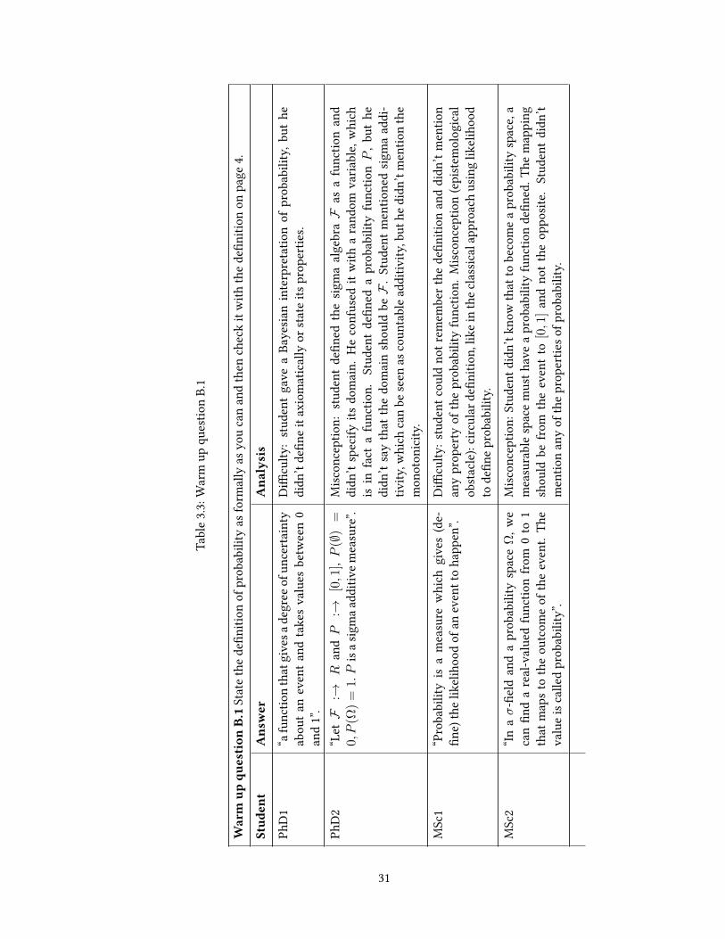
T abl

e3.3

:War

mup

ques

tion

B.1

Warm

upqu

estion

B.1

Stat

eth

ede

niti

onof

prob

abili

tyas

form

ally

asyo

uca

nan

dth

ench

eck

itw

ithth

ede

niti

onon

page

4.Stud

ent

Ans

wer

Ana

lysis

P hD

1“a

func

tion

that

give

sade

gree

ofun

certa

inty

abou

tan

even

tand

take

sva

lues

betw

een

0an

d1”

.

Di

culty

:st

uden

tga

vea

Baye

sian

inte

rpre

tatio

nof

prob

abili

ty,b

uthe

didn

’tde

ne

itax

iom

atic

ally

orst

ate

itspr

oper

ties.

P hD

2“L

etF

:→R

andP

:→[0,1

],P

(∅)

=0,P

(Ω)

=1.P

isas

igm

aadd

itive

mea

sure

”.M

iscon

cept

ion:

stud

ent

den

edth

esig

ma

alge

braF

asa

func

tion

and

didn

’tsp

ecify

itsdo

mai

n.H

eco

nfus

edit

with

ara

ndom

varia

ble,

whi

chis

infa

cta

func

tion.

Stud

ent

den

eda

prob

abili

tyfu

nctio

nP

,but

hedi

dn’t

say

that

the

dom

ain

shou

ldbeF

.St

uden

tmen

tione

dsig

ma

addi

-tiv

ity,w

hich

can

bese

enas

coun

tabl

eadd

itivi

ty,b

uthe

didn

’tm

entio

nth

em

onot

onic

ity.

MSc

1“P

r oba

bilit

yis

am

easu

rew

hich

give

s(d

e-n

e)th

elik

elih

ood

ofan

even

tto

happ

en”.

Di

culty

: stu

dent

coul

dno

trem

embe

rthe

den

ition

and

didn

’tm

entio

nan

ypr

oper

tyof

the

prob

abili

tyfu

nctio

n.M

iscon

cept

ion

(epi

stem

olog

ical

obst

acle

):ci

rcul

arde

niti

on,l

ikei

nth

ecla

ssic

alap

proa

chus

ing

likel

ihoo

dto

den

epr

obab

ility

.

MSc

2“In

aσ

-el

dan

da

prob

abili

tysp

ace

Ω,w

eca

nn

da

real

-val

ued

func

tion

from

0to

1th

atm

apst

oth

eou

tcom

eof

the

even

t.Th

eva

lue

isca

lled

prob

abili

ty”.

Misc

once

ptio

n:St

uden

tdid

n’tk

now

that

tobe

com

ea

prob

abili

tysp

ace,

am

easu

rabl

esp

ace

mus

thav

ea

prob

abili

tyfu

nctio

nde

ned

.The

map

ping

shou

ldbe

from

the

even

tto

[0,1

]an

dno

tthe

oppo

site.

Stud

entd

idn’

tm

entio

nan

yof

the

prop

ertie

sofp

roba

bilit

y.

31

T abl

e3.4

:War

mup

ques

tion

B.2

Warm

upqu

estion

B.2

Thin

kof

adi

e.W

hati

sthe

prob

abili

tyth

atyo

uw

illge

tthe

num

ber4

ina

roll

ofa

die?

Wha

tist

hepr

obab

ility

that

you

will

geta

nod

dnu

mbe

rin

aro

llof

adi

e?H

owdi

dyo

un

dth

ese

resu

lts?

Stud

ent

Ans

wer

Reasoning

Ana

lysis

P hD

21/

6an

d1/

2“1

=∑ 6 i=

1P

(Ai)

=6P

(A1)⇒

P(A

i)=

1/6,

cons

ider

ingt

hesy

mm

etry

ofth

edie

.Ana

logo

usw

ayto

the

1/2.”

Itw

asth

eon

lyst

uden

ttha

tdid

n’tm

entio

nth

ecl

as-

sical

appr

oach

.

All

the

othe

rst

uden

ts1/

6an

d1/

2Ra

tiobe

twee

nfa

vora

ble

and

poss

ible

case

s.A

llof

them

gave

corr

ectv

alue

soft

hepr

obab

ilitie

s,bu

tusin

gth

ecl

assic

alap

proa

ch.

Tabl

e3.5

:Que

stio

nB1

Que

stionB1

Thin

kof

aco

unta

bly

inn

itese

t.Ca

nw

eas

sign

prob

abili

tyto

each

elem

ento

fthi

sse

tby

the

ratio

betw

een

the

num

ber

offa

vora

ble

case

sand

the

num

bero

fall

poss

ible

case

s?Stud

ent

Ans

wer

Reasoning

Ana

lysis

PhD

1,Ph

D2

and

MSc

2N

oTh

eth

ree

parti

cipa

nts

pres

ente

dth

at,i

nth

isca

se,

fort

hesu

mto

conv

erge

,eac

hel

emen

tsho

uld

have

prob

abili

ty0,

soin

this

case

the

sum

wou

ldn’

tbe

1.

The

thre

epr

esen

ted

the

right

reas

onin

g.Th

eyw

ere

thin

king

abou

tcou

ntab

lead

ditiv

ity.

MSc

1y e

sTh

isst

uden

tco

uldn

’tan

swer

the

ques

tion

and

skip

ped

it.Bu

the

cam

eba

ckaf

ter

reso

lvin

gqu

es-

tion

5.H

esai

dit

wou

ldbe

:“Ye

sbec

ause

then

umbe

rof

elem

ents

ofth

ese

twou

ldbe

inn

ite”.

Di

culty

:st

uden

tw

asn’

tab

leto

expr

ess

his

thou

ghts

and

hego

tmor

eco

nfus

edw

hen

heca

me

back

toth

equ

estio

naf

terd

oing

ques

tion

5.

32

T abl

e3.6

:Que

stio

nB2

Que

stionB2

Isit

poss

ible

tode

ne

apr

obab

ility

func

tion

unifo

rmly

dist

ribut

edon

the

natu

raln

umbe

rs,N

?Stud

ent

Ans

wer

Reasoning

Ana

lysis

All

the

stu-

dent

sN

oFo

r the

sum

toco

nver

ge,e

ach

elem

ents

houl

dha

vepr

obab

ility

0,so

inth

isca

seth

esu

mw

ould

n’tb

e1.

The

four

pres

ente

dth

erig

htre

ason

ing.

They

wer

eth

inki

ngab

outc

ount

able

addi

tivity

.

Tabl

e3.7

:Que

stio

nB3

Que

stionB3

Wha

t,in

tuiti

vely

,ist

hepr

obab

ility

that

a“r

ando

mly

chos

en”n

atur

alnu

mbe

risa

mul

tiple

of3?

Stud

ent

Ans

wer

Reasoning

Ana

lysis

PhD

21/

3H

em

ade

apa

rtitio

nof

Nin

equi

vale

nce

clas

ses

ofth

enat

ural

num

bers

mod

(3).

Then

hese

tpro

babi

lity

1/3

for

each

clas

s,so

the

clas

sof

0(w

hich

are

the

mul

tiple

sof3

)wou

ldha

vepr

obab

ility

1/3.

This

answ

eris

mor

eso

phist

icat

edth

anth

ecl

assic

alap

proa

ch.H

espl

itth

enat

ural

num

bers

into

3equ

iv-

alen

cecl

asse

stha

thav

ethe

sam

ecar

dina

lity,

soth

eyar

esym

met

ricw

ithre

gard

sto

thec

ount

ing

mea

sure

.A

llth

eot

her

stud

ents

1/3

All

theo

ther

stho

ught

abou

tthe

ratio

betw

een

favo

r-ab

lean

dpo

ssib

leca

ses.

False

rule

:the

yal

lapp

lied

the

clas

sical

appr

oach

toan

inn

itese

t.

33

T abl

e3.8

:Que

stio

nB4

Que

stionB4

LetP

(3N

)be

the

prob

abili

tyth

ata

natu

raln

umbe

r,ra

ndom

lych

osen

in1,2,...,N,

isa

mul

tiple

of3.

Can

you

see

that

limN→∞P

(3N

)=

1/3?

Let’s

call

this

limitP

3.Th

isfo

rmal

izes

the

intu

ition

inqu

estio

nB3

,and

give

susa

way

toas

sign

“pro

babi

litie

s”to

certa

inev

ents

that

are

inn

itesu

bset

sofn

atur

alnu

mbe

rs.

Stud

ent

Ans

wer

Reasoning

Ana

lysis

P hD

21/

3H

em

ade

apa

rtitio

nof

Nin

equi

vale

nce

clas

ses

ofth

enat

ural

num

bers

mod

(3).

Then

hese

tpro

babi

lity

1/3

for

each

clas

s,so

the

clas

sof

0(w

hich

are

the

mul

tiple

sof3

)wou

ldha

vepr

obab

ility

1/3.

This

answ

eris

mor

eso

phist

icat

edth

anth

ecl

assic

alap

proa

ch.H

espl

itth

enat

ural

num

bers

into

3equ

iv-

alen

cecl

asse

stha

thav

ethe

sam

ecar

dina

lity,

soth

eyar

esym

met

ricw

ithre

gard

sto

thec

ount

ing

mea

sure

.A

llth

eot

her

stud

ents

1/3

All

theo

ther

stho

ught

abou

tthe

ratio

betw

een

favo

r-ab

lean

dpo

ssib

leca

ses.

False

rule

:the

yal

lapp

lied

the

clas

sical

appr

oach

toan

inn

itese

t.

34

T abl

e3.9

:Que

stio

nB5

Que

stionB5

IfA

isan

yse

tofn

atur

alnu

mbe

rs,l

etA

(N)

beth

enum

bero

fele

men

tsofA

whi

char

eles

stha

nor

equa

ltoN

.The

nde

note

the

“pro

babi

lity”

ofA

asP

(A)

=li

mN→∞A

(N)/N

prov

ided

this

limit

exist

s.W

hati

sthe

prob

abili

tyofA

,ifA

isn

ite?

And

ifA

isin

nite

?D

oyo

use

ean

yco

ntra

dict

ion

with

limN→∞P

(3N

)=

1/3

from

ques

tion

B4?

Stud

ent

Ans

wer

Reasoning

Ana

lysis

P hD

1A

nite

:0;

Ain

nite

:1;

No

cont

ra-

dict

ion.

“A(N

)/N→

0asN→∞

.N/N→

1asN→∞

.N

oco

ntra

dict

ion.”

The

rst

two

answ

ers

are

right

,how

ever

,the

reis

adi

cu

ltyw

hen

hedi

dn’t

see

the

cont

radi

ctio

n.H

esh

ould

see

that

coun

tabl

ead

ditiv

ityw

ould

n’tw

ork

fort

hesu

bset

sofN

.Ph

D2

An

ite:0

;Ain

nite

:no

answ

er.

No

cont

radi

c-tio

n.

He

saw

clea

rlyth

atw

henA

isn

ite,P

(A)

goes

toze

ro.

For

the

inn

iteca

se,h

est

arte

dan

argu

men

tus

ing

the

pow

erse

tofA

.Itri

edto

mak

eit

simpl

eran

dsa

id,i

nste

adof

age

neric

set,

thin

kof

N,a

ndhe

thou

ghtt

hatt

hepo

wer

seto

fNw

asa

subs

etof

it.

For

the

nite

case

hega

veth

erig

htan

swer

.Fo

rth

ein

nite

case

,the

rew

asa

misc

once

ptio

nth

atth

epo

wer

seto

fNw

asas

ubse

tofN

.Hes

awno

cont

ra-

dict

ion,

beca

use

hene

vert

houg

htof

the

prob

abili

tyw

ithth

ecl

assic

alap

proa

chin

the

prev

ious

case

s.

MSc

1A

nite

:0;

Inde

term

i-na

tion.

No

cont

radi

c-tio

n.

He

saw

clea

rlyth

atw

henA

isn

ite,P

(A)

goes

toze

ro.H

efou

ndth

atth

elim

itw

ould

bean

inde

term

i-na

teof

the

form∞/∞

,whi

chca

nbe

anyt

hing

.No

cont

radi

ctio

nbe

caus

eof

the

inde

term

inat

ion

foun

d.

For t

hen

iteca

seth

eans

wer

isrig

ht.F

orth

ein

nite

case

:di

culty

–in

stea

dof

taki

ngth

eca

rdin

ality

ofth

ese

tsto

esta

blish

N/N

and

nd

1as

are

sult,

hepu

t∞/∞

.

MSc

2A

nite

:0;

Inde

term

i-na

tion.

No

cont

radi

c-tio

n.

He

saw

clea

rlyth

atw

henA

isn

ite,P

(A)

goes

toze

ro.

He

foun

dth

atth

elim

itw

ould

bean

inde

ter-

min

ateo

fthe

form∞/∞

,whi

chca

nbe

anyt

hing

.“I

don’

thav

een

ough

argu

men

tsto

see

any

cont

radi

c-tio

n”.

Fort

hen

iteca

seth

eans

wer

isrig

ht.F

orth

ein

nite

case

:di

culty

–in

stea

dof

taki

ngth

eca

rdin

ality

ofth

eset

stoe

stab

lishN/N

and

nd1a

sare

sult,

hepu

t∞/∞

.Ast

hest

uden

tdid

n’ts

eeth

atth

elim

itw

as1

inth

ein

nite

case

,hec

ould

n’ts

eeth

econ

tradi

ctio

n.

35

T abl

e3.1

0:Q

uest

ion

B6

Que

stionB6

:Let

Ω=

N.I

sitt

rue

that

ifN

=∪∞ i

=1ni

,the

nP

(N)

=∑ ∞ i=

1P

(ni)

?

Stud

ent

Ans

wer

Reasoning

Ana

lysis

PhD

1Tr

ue“J

ustt

hink

ofco

unta

ble

addi

tivity

”.Th

ean

swer

isno

twro

ng,b

utth

ere

was

adi

cu

ltyin

stat

ing

the

prob

abili

tiesf

orea

chni,

that

was

not

done

.P h

D2

T rue

He

said

that

the

idea

isto

build

the

prob

abili

tyfo

rea

chni

inth

esam

eway

hebu

iltfo

rthe

mul

tiple

sof

3(w

itheq

uiva

lenc

ecl

asse

s)an

dth

en,t

hest

atem

ent

istru

e.

Di

culty

–th

est

uden

tdid

n’tg

etto

actu

ally

build

the

prob

abili

tyfo

rni

usin

geq

uiva

lenc

ecl

asse

s.H

eco

uldn

’tde

ne

thos

eeq

uiva

lenc

ecl

asse

s.

MSc

1Fa

lse“It

’sim

poss

ible

todo

itbe

caus

eif

eachni

have

the

sam

epr

obab

ility

,the

sum

dive

rges

”.Th

ean

swer

isco

rrec

t,bu

tin

com

plet

e,be

caus

ehe

coul

dde

ne

the

prob

abili

tylik

ea

geom

etric

serie

s:P

(ni)

=2−

ni

MSc

2Tr

ue“I

don’

tkno

who

wto

just

ifyit”

.

36

T abl

e3.1

1:Q

uest

ion

B7

Que

stionB7

We

know

that

:ifn

1,n

2,...,

isa

coun

tabl

ein

nite

sequ

ence

ofdi

sjoin

tsub

sets

ofF

,the

nP

(∪∞ i=

1ni)

=∑ ∞ i=

1P

(ni)

.Is

itco

mpa

tible

with

the

ques

tion

B6,i

nth

ese

nse

that

N=∪ i

=1ni,

thenP

(N)

=∑ ∞ i=

1P

(ni)

?

Stud

ent

answ

ers

Reasoning

Ana

lysis

PhD

2Tr

ueH

eus

edth

esa

me

argu

men

tasi

nqu

estio

nB6

.D

icu

lty–

the

stud

entd

idn’

tbui

ldth

epr

obab

ility

forn

ius

ing

equi

vale

nce

clas

ses.

He

coul

dn’t

den

eth

ose

equi

vale

nce

clas

ses.

MSc

1Fa

lse“F

orth

isto

betru

e,w

ew

ould

need

man

yni

with

prob

abili

ty0”

.D

icu

lty:

apo

sitiv

e,bu

tgeo

met

rical

lyde

crea

sing

prob

abili

tyw

ould

betru

eas

wel

l,ho

wev

erit

istru

eth

atfo

ri

larg

een

ough

,P

(ni)

wou

ldne

edto

besm

alle

rtha

nε.

MSc

2Tr

ue“I

don’

tkno

who

wto

just

ifyit”

.

37

T abl

e3.1

2:Q

uest

ion

B8

Que

stionB8

:Go

back

toqu

estio

nB1

.Hav

eyo

uch

ange

dyo

urm

ind?

Just

ify.

Stud

ent

Ans

wer

Reasoning

Ana

lysis

P hD

1Y e

s"I

chan

ged

my

min

dbe

caus

eac

cord

ing

toqu

estio

ns3,

4an

d5

we

can

build

this

prob

abili

ty".

Di

culty

: the

stud

entd

idn’

tund

erst

and

that

ques

-tio

nv

egi

ves

aco

ntra

dict

ion

with

the

way

ofas

-sig

ning

prob

abili

tyin

ques

tion

4fo

rin

nite

sets

.P h

D2

No

He

didn

’tse

ea

cont

radi

ctio

nbe

caus

efro

mth

ebe

-gi

nnin

ghe

was

alre

ady

thin

king

ofpr

obab

ility

asa

mea

sure

,ins

tead

ofa

clas

sical

appr

oach

.

MSc

1Y e

s“W

ithth

ew

ayw

ede

ned

prob

abili

tyin

ques

tion

4w

eca

nas

sign

prob

abili

tylik

ein

ques

tion

1.”D

icu

lty: t

hest

uden

tdid

n’tu

nder

stan

dth

atqu

es-

tion

ve

give

sa

cont

radi

ctio

nw

ithth

ew

ayof

as-

signi

ngpr

obab

ility

inqu

estio

n4

fori

nni

tese

ts.

MSc

1N

oN

oju

sti

catio

n.H

eco

uldn

’tju

stify

beca

use

hedi

dn’t

see

the

cont

ra-

dict

ion.

He

thou

ghth

ene

eded

mor

ein

form

atio

n.

38

3.5 Discussion

In part A, it’s surprising that the student who performed best with the denition of probability,

PhD2, got lost in question A1, that probability can’t be bigger than 1. Not only PhD2, but MSc1 also

fell into the proportionality obstacle, when they applied a linear reasoning in a situation where it

is not possible.

Regarding questions A2 to A5, both PhD students were aware of sets of measure zero and that

they can represent events which are not necessarily impossible. Both MSc students were not sure

about these results and made mistakes about probability 0 and impossibility or probability 1 and

certainty of events.

In part B, the rst result that calls attention is that PhD2 is the student with most familiarity

with probability. He was the only one who, since the beginning, used the modern approach in-

stead of the classical one. This explains why he could see clearly that it’s not possible to dene

a probability with the classical approach in an innite set. He made some mistakes through the

interview but this can be attributed to distraction or lack of concentration.

MSc1 was the student that has shown the most contradictory answers. In Part B, he had dif-

culty answering question 1 and chose to skip it and move ahead, but then correctly answered

question 2, which focuses on a very similar idea.

PhD1, MSc1 and 2 gave answers at the same level of comprehension. They took a classical

approach in question 3 and didn’t see the contradiction of this approach to countably innite sets.

Also, PhD1 and MSc2 started with the idea that it is not possible to give a uniform probability

to the natural numbers, but they changed their minds when they didn’t identify the contradiction

between questions 4 and 5 and countable additivity. The element that was clear to them is that the

sum of the probabilities must be no greater than 1.

All the four students fell into the illusion of linearity and/or the obstacle of equiprobability,

which, despite the limitations of this pilot study, indicates a future research direction. The persis-

tance of those epistemological obstacles also made us curious about the approach that textbooks

advance most. After the interview, We reviewed with them the questions comparing their answers

to the expected ones as a form of feedback. PhD2 said that he had a lot of fun during this interview

because the subject was very interesting. The other three students were all glad that they had par-

ticipated in the interview, and all four said that they had learned something about probability as a

39

result of the questions.

The results found in this study is that students think of probability using the classical approach,

however, as demonstrated by PhD2, this view can change as you mature in the subject. Another

surprising result to us is that the epistemological obstacles of the illusion of linearity and equiprob-

ability are persistent among these graduate students. Nevertheless, caution must be taken, because

this is just a pilot study with only four students. These results must be seen as a rst insight into

the questions discussed here, and using them to make inferences about a wider population would

be another epistemological obstacle in probability, called law of small numbers [57]! This happens

when the results of a small and non-representative sample are extrapolated to a big population.

3.6 Final remarks

This pilot study was conceived to explore graduate student’s conceptualization of probability.

Regarding the approach they use in probability, it was shown that, except the student nishing

her/his PhD research in probability, all the others graduate students are more inclined to a classical

than to a modern one. Their answers pointed to confusion when asked to deal with innite sets. In

particular, contradictions were found on whether it is possible or not to use the classical approach

to assign probability to innite sets. This puts in evidence the persistence of the epistemological

obstacles of equiprobability and proportionality, that are associated to a classical reasoning in

probability.

This experiment can be improved in some ways. A bigger and more diversied sample with

students from other domains that use a lot of probability can always bring better and safer insights.

Also, if the student is certain that in question 5 of part B if the probability is 1 when A is an

innite set, and if we relate it more clearly with countable additivity, the quality of the answers

for analysis may be improved, because these items are essential to nd a contradiction with the

classical approach of probability in innite spaces.

40

Chapter 4

Classical Probability: The Origins, Its

Limitations and the Path to the

Modern Approach

4.1 Introduction

In this chapter, we want to discuss why probability became attached to measure theory at the

beginning of the 20th century. More specically, we are interested in knowing why probability

needed measure theory as its basis to be considered an autonomous branch of mathematics. While

probability has been present in various branches mathematics for many centuries, it was not until

the development of measure theory in the late 19th and early 20th century that probability could

be developed in full mathematical rigour. Following the work of such mathematicians as Borel,

Lebesgue and Fréchet, a strong relationship between probability and measure theory became ap-

parent.

If probability existed for centuries in mathematics before the development of measure theory,

why did the former needed the latter to constitute its basis? Which mathematical problems of the

time relied on the understanding of probability as a measure? What was the motivation for this

theoretical view change in probability, which had driven an association of probability and measure

at the very early stage of development of measure theory?

Science doesn’t progress in a linearly path. From one advance to a new discover, there is a

41

myriad of distinct paths by which to continue, many of them leading down wrong turns, labyrinths

of blind alleyways, or dead ends. This road, full of sinuous curves makes the progress of science

slow. For example, Borel was studying convergence of series in complex analysis when he rst

forayed into measure theory. Rather than proceeding with a purely chronological exposition, we

will explore the main ideas, even the blind alleyways, that led to the axiomatization of probability

based on measure theory.

Prior to Kolomogorov’s axiomization of probability in 1933, classical probability was consid-

ered a branch of applied mathematics. It provided formulas for error terms, economic activities,

statistical physics and solutions to problems in games of chance. This non-mathematical context

was related to combinatorics and dierential equations among others. Despite the advances in

classical probability, not much attention was given to the mathematical basis of that probabilis-

tic context, and the subject was not yet considered an autonomous branch of mathematics. It was

connected with a nite number of alternative results of a trial that are considered equiprobable but

"... even the real world does not possess the absolute symmetries of the classical theory’s equipossible

cases" [67] (p. 6). The concepts and methods were specic to applications, and their contributions

to larger questions of science and philosophy were limited. Regarding the mathematical point of

view, there was a need for the denition and foundation of probability using a general and abstract

approach. Before this formalization could be achieved, the development of measure theory was

necessary, so probability could use it as the ground for its modern foundations and to become an

autonomous mathematical discipline as we will see in the following sections.

In a broader perspective, the shift from classical to modern probability appears as part of a

greater movement, the very change from classical to modern science itself. Von Plato [67] saw

that it would be necessary to nd a scenario requiring the development of the concepts of chance

and statistical law, for probability to become an autonomous branch of mathematics. Although

mathematicians had begun looking for a formal and abstract denition of probability before the

turn of the century, it was not until the quantum mechanical revolution between 1925 and 1927,

that the abstract study of probability became necessary for further scientic advancement. Quan-

tum mechanics viewed the elementary processes in nature as non-deterministic, with probability

playing an essential role in describing those processes. In its relation to physics, probability had

many technical developments motivated by statistical physics, however the foundation for the de-

velopment of modern probability found a ground in quantum mechanics, studied by Hilbert and

42

Kolmogorov himself.

In this chapter, we will discuss the development of the set of axioms for probability based

on measure theory, that is, a very deep change in the basis of probability that took it from a

set of tools to solve problems from physics, gambling, economics, and other human activities to

an autonomous branch of mathematics. This period in the history of probability is analyzed by

Shafer and Vovk [56]. They advocate that Kolmogorov’s work in establishing a set of axioms was

a product of its time, in the sense that the emergence of these ideas does not stem exclusively from

Kolmogorov’s originality, but is due to the presence of the work of many of his predecessors. We

will use the historical approach used by Shafer and Vovk as a guideline, however our study will

explore a narrower account of history, focusing only on those fewer ideas that we consider to be

key concepts in the establishment of the axioms and providing for these results a more detailed

mathematical exposition. We will occasionally detail succinct proofs from their original sources,

providing insight to make them more accessible and closer to today’s language.

Another important source in this subject is the book of Von Plato [67]. He presents many prob-

lems that motivated the development of probability as well as some philosophical questions. His

approach diers from this chapter in that it is more concerned with the development of the phi-

losophy and the concepts of probability in connection to statistical and quantum physics. We have

chosen to focus instead on the mathematical features of the development of modern probability.

The philosophy and dierent interpretations of probability, although very interesting subjects, go

beyond the scope of our work and can be themes for another thesis.

In the next section, we will concern ourselves with probability before to the 20th century.

We will discuss the origins of probability, the denition of classic probability of Bernoulli and De

Moivre that remained essentially stable until the birth of measure theory, and Bayes’ contribu-

tion for the cases involving the dependence of events. The third section presents the development

of measure theory, with focus on the results that were important to the development of modern

probability. In the last section we will discuss the natural association of probability to measure

theory, present since its inception with the work of Borel and Lebesgue. We will explain the asso-

ciation of both disciplines, the need to develop a general and abstract set of axioms for probability

and the rst attempts at an axiomatization. We will also discuss Borel’s denumerable probability,

more specically the use of countable additivity and the strong law of large numbers, two essential

results to the foundation of the axioms.

43

4.2 Probability before 1900

In this section, we start by presenting the origins of probability and its establishment to the

status of a science. We present Bernoulli’s book, Ars Conjectandi, focusing on two features that

are central to this thesis: i) the classical denition of probability and ii) Bernoulli’s law of large

numbers, which was the rst convergence theorem in probability that was presented and proved

with complete analytic rigour. After Bernoulli’s work we present the work of De Moivre, The

Doctrine of Chances, and conclude with Bayes’ contribution to conditional probability with the

theorem that carries his name.

4.2.1 The origins of probability

It is widely accepted that the birth of and early developments in probability theory arose from

gambling. Even without denying the importance of gambling to the development of probability

techniques, Maistrov [46] asserts that probability theory could emerge only after the problems con-

nected with probabilistic estimation from several elds of human activity became more pressing.

The turn of the century brought about a period of the collapse of feudal relations, proletarization

of peasants and the rise of the bourgeoisie, resulting in a period of growth of cities and commerce.

At this time, problems in demography, insurance business, observational errors and many statis-

tical problems which arose as a result of the development of capitalistic relations and presented a

decisive stimulus for the birth of probability. The development of the capitalistic system, with its

monetary form of exchange, led to games of chance becoming a mass phenomenon with analogous

problems raised in other elds of human endeavour behind them.

From a mathematical point of view, the birth of probability coincided with the development

of analytic geometry, dierential and integral calculus and combinatorics. Up to the middle of

the 17th century, no general method for solving probabilistic problems was available. There were

many materials resulting from various branches of human activity related to probabilistic topics,

but a theory of probability had not being created yet. To exemplify, back in the 16th century,

Cardano was able to calculate the number of possible outcomes with and without repetition in the

case of two and three dice throws. He approached the notion of statistical regularity and came

close to a denition of probability in terms of the ratio of equal probability events using the idea

of mathematical expectation. Around mid-17th century, Pascal, Fermat and Huygens applied the

44

addition1 and multiplication2 rules of probability and were familiar with the notions of dependence

and independence of events and mathematical expectation. However, these ideas were developed

only in the simplest cases, and appeared as solutions to particular problems rather than going

further into the development of concepts and rules as general statements [46].

Even though there remains to be a general consensus in mathematics, in this thesis we consider

Bernoulli and De Moivre as the founders of classical probability. Both these authors acknowledged

the works of Cardano and Tartaglia, Fermat, Pascal, Huygens and Montmort among others in their

books, but they came up with a greater level of generality. Unlike Cardano, Bernoulli was able to

dene probability as a ratio, and De Moivre saw that the results achieved in Montmort’s work

may be derived from a general theorem. What leads us to crediting Bernoulli and De Moivre with

creating the foundation for probability as a science is the fact that they were the rst to dene

probability and expectation with a greater level of generality. Also, while Bernoulli presented and

proved with complete analytic rigour the rst convergence theorem in probability, De Moivre was

aware of the general results that before him were applied to only specic problems [30].

Now that we have briey discussed the origins of classical probability and mentioned the main

authors of that period, we present the Ars Conjectandi of Bernoulli and his denition of probability

as a ratio of favourable to possible cases. This denition became the classical standard one used

from the beginning of the 18th century until the rupture with the classical approach in 1933 with

Kolmogorov’s axioms of modern probability.

4.2.2 Bernoulli’s Ars Conjectandi and the denition of probability

Jacques Bernoulli, also known as Jacob and James, was born in Basel, Switzerland, in 1654 and

died in 1705. Bernoulli received his Master of Arts in philosophy in 1671, a licentiate in theology

in 1676 and studied mathematics and astronomy. In his works, he made many contributions to

calculus, and is one of the founders of calculus of variations. However, his greatest contribution

was in the eld of probability, where he derived the rst version of the law of large numbers in

his work Ars Conjectandi [26].

Bernoulli’s book “Ars Conjectandi” (The art of Conjecturing), was published eight years after

his death by his nephew Nicholas Bernoulli. This book played such a signicant role in the history1The addition rule can be stated as: P (A ∪B) = P (A) + P (B) if A and B can’t both happen simultaneously.2The multiplication rule can be stated as: P (A ∩B) = P (A) · P (B|A).

45

of probability, that thanks to this work, probability began a new era in its development and was

raised to the status of a science.

Ars Conjectandi is divided into four parts. The rst one, “A Treatise on Possible Calculations

in a Game of Chance of Christian Huygens with J. Bernoulli’s Comments”, consists of a reprint of

Huygens work (De Ratiocinniis in Ludo Aleae) accompanied by Bernoulli’s comments in all but

one proposition. In his commentary on the 12th proposition, he establishes the result known as

Bernoulli’s formula for the binomial distribution.

The second part of the book is called “The Doctrine of Permutations and Combinations”. Having

one entired part of his book dedicated to combinatorics gives an evidence to the extent of the usage

this discipline as a basic tool for probability before the introduction of innitesimal analysis.

The third part is called “Applications of the Theory of Combinations to Dierent Games of Chance

and Dicing”. He presents 24 problems, some of them solved in their general form rather than

through a numerical approach. Even though these three parts made a signicant contribution not

only to probability, but to mathematics as a whole, the most important part of the book that marks

a new era in probability history is the last one.

The fourth and last part, “Applications of the Previous Study to Civil, Moral and Economic Prob-

lems”, was left incomplete in the sense that he didn’t write about the applications in the title. This

part explains his interpretation of probability and also contains the proof of Bernoulli’s theorem,

that is, the weak law of large numbers in its simplest form.

Regarding his denition of probability, Bernoulli states it in the classical way, as the ratio

between favourable and possible outcomes. Nevertheless, he is conscious that “... this by no means

takes place with most other eects that depend on the operation of nature or on human will”. Thus,

for the cases which we can’t regard as equally likely to occur, or for which we can’t a priori have

an idea of its probability, because we don’t know the number of favourable and possible outcomes,

Bernoulli states we can still nd the probability “... a posteriori from the results many times observed

in similar situations, since it should be presumed that something can happen or not to happen in

similar circumstances in the past” [7] (p. 326-327). However, Bernoulli calls attention to a possible

misunderstanding. He mentions that the ratio we are seeking to determine through observation

is only approximate, and can never be obtained with absolute accuracy. "Rather, the ratio should

be dened within some range, that is, contained within two limits, which can be made as narrow as

anyone might want" [7] (p. 329).

46

Following these explanations, Bernoulli goes to chapter 5 of the 4th part of his book, where

he states ve lemmas and proves his theorem. We will present each of Bernoulli’s ve lemmas, as

well as his principal proposition, or theorem, the weak law of large numbers. We will also present

the ideas of Bernoulli’s proofs, however using modern language and notation. The statement of

each of the ve lemmas and the principal proposition are all taken directly from Ars Conjectandi.

[7].

4.2.3 Bernoulli’s law of large numbers

Lemma 4.2.1. Consider the two series of numbers:

0, 1, 2, 3, 4, ..., r − 1, r, r + 1, ..., r + s

0, 1, 2, 3, 4, . . .︸ ︷︷ ︸A

, nr − n, . . .︸︷︷︸B

, nr, . . .︸︷︷︸C

, nr + n, . . . , nr + ns︸ ︷︷ ︸D

.

• We can notice that the second series has n times more elements than the rst one and each

element of the rst series can be multiplied by n and linked to an element in the second one;

• As we increase n, the number of terms in the parts B, C and between 0 and nr will increase;

• Also, no matter how large n is, the number of terms in D won’t be larger than the number of

terms in B times (s− 1) or the number of terms in C times (s− 1).

• In the same way, the number of terms in A won’t be larger than the number of terms in B times

(r − 1) or the number of terms in C times (r − 1).

We will omit the demonstration of this rst lemma because the reader can simply verify it by

some simple arithmetic calculations.

Lemma 4.2.2. Every integer power of a binomial r+s is expressed by onemore term than the number

of units in the index of the power.

In this lemma, Bernoulli meant that, when n is an integer, the expansion of (r+ s)n has n+ 1

terms. This can be veried by induction.

Lemma 4.2.3. In any power of this binomial (at least in any power of which the index is equal to the

binomial r + s = t, or to a multiple of it, that is, nr + ns = nt), if some terms precede and others

47

follow some termM such that the number of all the preceding terms to the number of all the following

terms is, reciprocally, as s to t (or, equivalently, if in that term the numbers of dimensions of the lefters

r and s are directly as the quantities r and s themselves), then that term will be the largest of all the

terms in that power, and the terms nearer it on either side will be larger than the terms farther away

on the same side. But this same termM will have a smaller ratio to the terms closer to it than those

nearer terms (in an equal interval of terms) have to the farther terms.

The idea of the lemma is to show the binomial expansion of (r + s)nr+ns. By lemma (4.2.2),

its expansion has nr + ns+ 1 terms:

rnt+nt

1rnt−1s+

nt(nt− 1)

1 · 2rnt−1s2 + · · ·︸ ︷︷ ︸

ns terms

+M + · · ·+ nt

1rsnt−1 + snt︸ ︷︷ ︸

nr terms

.

Bernoulli also states that M will be the largest term, and that the terms closer to M will be

larger than those farther from it. Furthermore, the ratio between consecutive terms closer to M

will be smaller than the ratio of consecutive terms farther from M .3

Proof. Note that the coecients of the terms equidistant from the ends are the same. To see that

there are ns terms before M and nr terms after M , note that by lemma (4.2.2), the expansion has

nr + ns terms plus the term M . So he states that the ratio of terms preceding M by the terms

after M must be the same as s/r, and this implies that we have ns terms before M and nr terms

after M .

So we can say that

M =nt(nt− 1)(nt− 2) · · · (nt− ns+ 1)

1 · 2 · 3 · 4 · · ·nsrnrsns =

nt(nt− 1)(nt− 2) · · · (nr + 1)

1 · 2 · 3 · 4 · · ·nsrnrsns

=nt(nt− 1)(nt− 2) · · · (nt− nr + 1)

1 · 2 · 3 · 4 · · ·nrrnrsns =

nt(nt− 1)(nt− 2) · · · (ns+ 1)

1 · 2 · 3 · 4 · · ·nrrnrsns

We can express the two neighbours of M on the left and right in the binomial expansion as:3The same is valid for non-consecutive terms. For example, the ratio between the 3rd and the 6th term fromM will

be larger than that of of the 10th and the 13th term from M .

48

nt(nt− 1)(nt− 2) · · · (nr + 3)

1 · 2 · 3 · 4 · · · (ns− 2)rnr+2sns−2 +

nt(nt− 1)(nt− 2) · · · (nr + 2)

1 · 2 · 3 · 4 · · · (ns− 1)rnr+1sns−1 +M

+nt(nt− 1)(nt− 2) · · · (ns+ 2)

1 · 2 · 3 · 4 · · · (nr − 1)rnr−1sns+1 +

nt(nt− 1)(nt− 2) · · · (ns+ 3)

1 · 2 · 3 · 4 · · · (nr − 2)rnr−2sns+2

Now we divide the neighbours as per the items bellow and we can draw the conclusion of the

lemma:

(1) Dividing M by the term on its left, we get: (nr+1)sns·r and (nr+ 1)s > ns · r, which implies M

is bigger than its left neighbor.

(2) Dividing the rst M left neighbor by the next left neighbor we get: (nr+2)s(ns−1)r and (nr+ 2)s >

(ns− 1)r, so the rst left neighbor is greater than the second one.

(3) Dividing M by the term on its right, we get: (ns+1)rnr·s and (ns+ 1)r > nr · s, so M is bigger

than its right neighbor.

(4) Dividing the rst M right neighbor by the next right neighbor we get: (ns+2)r(nr−1)s and (ns +

2)r > (nr − 1)s, so the rst right neighbor is greater than the next one.

Doing this procedure recursively, we can gure out that M is the greatest element in the

expansion and the elements reduce as they get farther from M .

We can also notice that (nr+1)sns·r < (nr+2)s

(ns−1)r and that (ns+1)rnr·s < (ns+2)r

(nr−1)s . So doing this procedure

recursively we can see that M has smaller ratios to nearer terms than to further ones on the same

side.

Lemma 4.2.4. In a power of a binomial with index nt, the number n can be conceived to be so large

that the largest termM acquires a ratio to the terms α and β, which are at an interval of n terms to

the left and right of it that is larger than any given ratio.

The goal of this lemma is to show that: limn→∞Mα =∞ and limn→∞

Mβ =∞.

Proof.

M =nt(nt− 1)(nt− 2) · · · (nr + 1)

1 · 2 · 3 · 4 · · ·nsrnrsns =

nt(nt− 1)(nt− 2) · · · (ns+ 3)

1 · 2 · 3 · 4 · · · (nr − 2)rnr−2sns+2

49

On the left,

α =nt(nt− 1)(nt− 2) · · · (nr + n+ 1)

1 · 2 · 3 · 4 · · · (ns− n)rnr+nsns−n

On the right,

β =nt(nt− 1)(nt− 2) · · · (ns+ n+ 1)

1 · 2 · 3 · 4 · · · (nr − n)rnr−nsns+n

Now we can put the ratios:

M

α=

(nr + n)(nr + n− 1)(nr + n− 2) · · · (nr + 1)sn

(ns− n+ 1)(ns− n+ 2)(ns− n+ 3) · · ·ns · rn

=(nrs+ ns)(nrs+ ns− s)(nrs+ ns− 2s) · · · (nrs+ s)

(nrs− nr + r)(nrs− nr + 2r)(nrs− nr + 3r) · · ·nrs

M

β=

(ns+ n)(ns+ n− 1)(ns+ n− 2)...(ns+ 1)rn

(nr − n+ 1)(nr − n+ 2)(nr − n+ 3)...nr · sn

=(nrs+ nr)(nrs+ nr − r)(nrs+ nr − 2r)...(nrs+ r)

(nrs− ns+ s)(nrs− ns+ 2s)(nrs− ns+ 3s)...nrs

As n goes to innity, the numbers (nr± n± 1), (nr± n± 2), ... and the numbers (ns± n±

1), (ns± n± 2), ... will all have the same values of (nr± n) and (ns± n). Now we can say that:

M

α=

(rs+ s)(rs+ s)...rs

(rs− r)(rs− r)...rs

As we have n factors both in the numerator and in the denominator, we have that: Mα =(

rs+srs−r

)n, which is an innitely large value. Similarly, we have that limn→∞

Mβ =∞.

Lemma 4.2.5. Given what has been posited in the preceding lemmas, n can be taken to be so large

that the sum of all the terms between the middle and maximum term M and the bounds α and β

inclusively has to the sum of all the remaining terms outside the bounds α and β a ratio larger than

any given ratio.

In other words, Bernoulli is stating that the ratio of the sum of all terms from α up to β to the

sum of all the remaining terms may be made arbitrarily large as n increases.

Proof. Out of the terms betweenM and the boundα. Let’s call the second term from the maximum

F , the thirdG, the fourthH and so on, and let the rst term to the left of α be called P , the second

50

one Q, the third R. So the terms could be placed like: ...R,Q, P, α, ...,H,G, F,M, .... Now,

from lemma (4.2.3) we have: MF < α

P ; FG < PQ ; GH < Q

R and so forth. We can also conclude thatMα < F

P < GQ < H

R and so successively.

From lemma (4.2.4), n → ∞ ⇒ Mα → ∞ as do the fractions F

P ; GQ ; HR ... . So we can conclude

that n → ∞ ⇒ F+G+H+...P+Q+R+... → ∞. So the sum of the terms between M and α is innitely larger

than the sum of the same number of terms to the left of α. But by the lemma (4.2.1), the number

of terms to the left of α doesn’t exceed (s− 1) times the number of terms between M and α, that

is, a nite number of times. Also, by lemma (4.2.3), the terms become smaller as they approach the

extremes, that is, farther to the left of α. We can see that the sum of the terms between M and α

will be innitely larger than the sum of all the terms beyond α. The same can be said about the

terms between M and β. Finally, the sum of the terms between α and β will be innitely larger

than the sum of all the other terms.

After this proof, Bernoulli also presents an alternative way of proving the lemmas (4.2.4) and

(4.2.5) because he was concerned about the reception of the idea that when n goes to innity, the

numbers (nr ± n ± 1), (nr ± n ± 2), ... and the numbers (ns ± n ± 1), (ns ± n ± 2), ... will all

have the same values of (nr ± n) and (ns± n), as presented in lemma (4.2.4).

Bernoulli shows that for any given (large) ratio c, we can nd a nite n such that the ratio of

the sum of the terms between the bounds α and β to all the other terms (the terms in the queue)

will be larger than c.

So for any value c, we can nd a nite n such that if we take the binomial (r + s)n with its

terms represented as:

a, · · · , f, g, h︸ ︷︷ ︸n(s−1) terms

,α, · · · , F,G,H︸ ︷︷ ︸n terms

,M, U, V,W, · · · ,β︸ ︷︷ ︸n terms

, u, v, w, · · · , z︸ ︷︷ ︸n(r−1) terms

,

it is true that α+...+F+G+H+M+U+V+W+...+βa+...+f+g+h+u+v+w+...+z > c.

To show this result, let’s take a ratio which is smaller than rs+srs−r . For example, we can take

r+1r = rs+s

rs < rs+srs−r . Now, we multiply this ratio r+1

r by itself as many times as necessary to make

it greater than or equal to c(s− 1), say k times, so we get(r+1r

)k ≥ c(s− 1).

Now, looking at the ratio Mα = (nrs+ns)

(nrs−nr+r) ·(nrs+ns−s)(nrs−nr+2r) ·

(nrs+ns−2s)(nrs−nr+3r) · · ·

(nrs+s)nrs , each indi-

vidual fraction is less than (rs+s)(rs−r) , but each of these individual fractions approaches (rs+s)

(rs−r) as n

51

increases.

Then we can see that among these fractions, the product of which gives Mα , one of them will

be rs+srs or equivalently r+1

r . Let’s nd the value of n such that the fraction in the kth position will

be equal to r+1r .

M

α=

(nrs+ ns)

(nrs− nr + r)︸ ︷︷ ︸1st position

· (nrs+ ns− s)(nrs− nr + 2r)︸ ︷︷ ︸

2nd position

· (nrs+ ns− 2s)

(nrs− nr + 3r)︸ ︷︷ ︸3rd position

· · · nrs+ ns− ks+ s

nrs− nr + kr︸ ︷︷ ︸kth position

· · · (nrs+ s)

nrs︸ ︷︷ ︸nth position

The fraction in the kth position is nrs+ns−ks+snrs−nr+kr . Now we nd n by: nrs+ns−ks+s

nrs−nr+kr = r+1r ⇒

n = k + ks−sr+1 and nt = kt+ kst−st

r+1 .

We will show that when the binomial (r + s) is raised to the power nt = kt + kst−str+1 , the

maximum term M will exceed the bound α more than c(s− 1) times, that is M > αc(s− 1), orMα > c(s− 1).

Too see this, note that the fraction in the kth position raised to the power k is, by construction,

greater than c(s− 1), that is: ( r+1r )k > c(s− 1).

The fraction in the preceding positions are all greater than the one in the kth position, then

(nrs+ ns)

(nrs− nr + r)︸ ︷︷ ︸1st pos

· (nrs+ ns− s)(nrs− nr + 2r)︸ ︷︷ ︸

2nd pos

· · · r + 1

r︸ ︷︷ ︸kth pos

>r + 1

r· r + 1

r· · · r + 1

r︸ ︷︷ ︸k times

= (r + 1

r)k > c(s− 1)

and we can conclude that the product of all the individual fractions will be even greater, so we can

say that: Mα > c(s− 1).

Looking at the expansion of the binomial, by lemma (4.2.3), we can say that Mα < Hh < G

g <Ff

and so successively, until the ratio of the last term in the bound, α, and its correspondent term

outside the bound (the nth term to the left of α) that we will call dα. Now, M > αc(s− 1) implies

thatH > hc(s−1), G > gc(s−1), F > fc(s−1), ..., α > dαc(s−1) . Now, summing the terms

in the left and in the right of these inequalities yields:

H +G+ F + ...+ α > hc(s− 1) + gc(s− 1) + fc(s− 1) + ...+ dαc(s− 1)

= (h+ g + f + ...+ dα)c(s− 1)

Finally, as we have n terms inside the bound and n(s − 1) terms in the left tail, we can conclude

52

that: M +H +G+ F + ...+ α > c(h+ g + f + ...+ a) or M+H+G+F+...+αh+g+f+...+a > c.

Bernoulli develops the same argument for the terms on the right side of M , and nds that the

n multiplied by t that will accomplish this task is: kt + krt−rts+1 . So taking the maximum between

this term and kt+ kst−str+1 we can conclude, nally, that: α+...+F+G+H+M+U+V+W+...+β

a+...+f+g+h+u+v+w+...+z > c.

Now that all the 5 lemmas have been demonstrated, Bernoulli nally presents his principal

proposition, which is stated and demonstrated below. Just a brief clarication of the language

used: what Bernoulli called fertile cases is equivalent to favourable cases in today’s terminology,

with sterile cases being the complement of the former.

Theorem 4.2.6. Let the number of fertile [or favourable] cases and the number of sterile [or non

favourable] cases have exactly or approximately the ratio r/s, and let the number of fertile cases to

all the cases be in ratio rr+s or r/t, which ratio is bounded by the limits r+1

t and r−1t . It is to be shown

that so many experiments can be taken that it becomes any given number of times (say c times) more

likely that the number of fertile observations will fall between these bounds than outside them, that is,

the ratio of the number of fertile to the number of all the observations will have a ratio that is neither

more than r+1t nor less than r−1

t .

Proof. Let’s consider nt to be the number of observations.

The probability of having 0, 1, 2, 3, . . . failures is expressed by:

rnt

tnt,

nt

tnt · 1rnt−1s,

nt(nt− 1)

tnt · 1 · 2rnt−2s2,

nt(nt− 1)(nt− 2)

tnt · 1 · 2 · 3rnt−3s3, . . .

Doing this procedure recursively, we can see that these are the terms in the expansion of the

binomial (r + s) raised to the power nt divided by tnt. Furthermore, the probability of having

nr favourable cases and ns non favourable cases is represented by the term M in the binomial

expansion (divided by tnt), and the probability of having nr + n or nr − n favourable cases is

associated to the bounds α and β.

The sum of the cases for which we have not more than nr + n and not less than nr − n

favourable occurrences is expressed by the sum of the terms of the power contained between the

bounds α and β.

The power of the binomial can be taken to be great enough, so the sum of the terms included

between the bounds α and β exceeds more than c times the sum of the terms in the tail. So we

53

can take a large number of observations such that the sum of the cases in which the ratio of

the number of favourable observations to the total number of observations will be between nr−nnt

and nr+nnt (or equivalently r+1

t and r−1t ), will exceed the sum of the remaining cases by more

than c times.

In Bernoulli’s own words, "it is rendered more than c times more probable that the ratio of the

number of fertile observations to the number of all the observations will fall within the bounds r+1t

and r−1t than that it will fall outside" (p. 338-339).

After this demonstration, Bernoulli gives an example where he gives values to r, s and c and

he nds the total number of observations n according to his theorem.

In his example he sets: r = 30, s = 20, t = r + s = 50 and c = 1000.

To the left side, (r + 1

r)k ≥ c(s− 1)⇒ k ≥ log[c(s− 1)]

log(r + 1)− log r=

4.2787536

142405= 301.

nt = kt+kst− sr + 1

< 24, 728.

To the right side, (s+ 1

s)k ≥ c(r − 1)⇒ k ≥ log[c(r − 1)]

log(s+ 1)− log s=

4.4623980

211893= 211.

nt = kt+krt− rs+ 1

< 25, 550.

If 25,550 trials were performed, it will be more than 1000 times more likely that the ratio of

favourable to the total number of observations will be between the bounds: 31/50 and 29/50 than

outside these bounds.

In modern notation, Bernoulli’s theorem can be stated as: if the probability of occurrence of

an event A in a sequence of n independent trials is p, and the total number of favourable cases

is m, then for any positive ε, one can assert with probability as close to 1 as desired, that for

a suciently large number of trials n, the dierence m/n − p is less than ε in absolute value:

P|m/n− p| < ε > 1− η, where η is an arbitrarily small number [46] (p. 74).

In this case, m/n is the empirical result of the trials and p is the M th term in the binomial

expansion. So the dierence between the estimation and the true probability measure could be

54

made arbitrarily small by raising the number of Bernoulli trials.

We need to clarify here that in Bernoulli’s theorem, no matter how large we choose n to be,

it is still possible to nd instances in a sequence of n trials in which the dierence |(m/n) − p|

is greater than ε. However, Bernoulli’s theorem guarantees that for n suciently large, in the

majority of cases, the inequality |(m/n) − p| < ε will be satised (or we can say that the set of

divergent points has measure zero) [46] (p. 74).

Hald [30] (p. 263) mentions that Bernoulli’s theorem is very important for probability theory,

because it gives a theoretical and rigorous justication for the usage of an estimator for a probabil-

ity, however, it doesn’t say how to nd an interval for the probability p from an observed value of

m/n because the total number of observations depends on p, t and c. On the other hand, Maistrov

[46] (p. 75) argues that the theorem doesn’t state that limn→∞m/n = p rather, it states that the

probability of large deviations of the frequencym/n from the probability p is small, if the number

of trials n is large enough.

4.2.4 De Moivre’s work - The Doctrine of Chances

Abraham de Moivre was born in Vitry-le-François, France, in 1667 and died in London, in

1754. He was one of the many gifted Protestants who emigrated from France to England. While

his formal education was in French, his many contributions were made within the Royal Society

of London. His father, a provincial surgeon of modest means, assured him of a competent but

undistinguished classical education. He read mathematics almost in secret, and Christiaan Huy-

gens’ work on the mathematics of games of chance, De ratiociniis in ludo aleae, formed part of this

clandestine study [26].

He dedicated his masterpiece, The Doctrine of Chances, to his friend Newton, and this book

became the standard knowledge of probability at that time. Among his contributions, we can list

his approximation to the binomial probability distribution. Bernoulli proved the weak law of large

numbers, and De Moivre’s approximation to the binomial distribution was conceived as an attempt

to improve this result. Bernoulli did some numerical examples of a binomial approximation for

particular values of n and p, but De Moivre was able to state the approximation to the binomial

distribution in a more general way.

As mentioned before, along with Bernoulli’s work, De Moivre’s work is also of crucial im-

portance, because the concepts they developed with attained a degree of generality that raised

55

probability theory to the status of science. De Moivre’s book, The Doctrine of Chances, brings a

denition of probability, some elementary theorems and some important advances in probabil-

ity techniques. For example, it improved the ways of calculating tails of binomial probabilities

brought by Bernoulli, which led to new proofs of the law of large numbers, and precise statements

for local and for integral limiting theorems [59]. However, for the purpose of this thesis we are

interested in the denition of probability and in the theorems of total probability (or the addition

theorem) and compound probability (or the multiplication theorem).

Just like Bernoulli, De Moivre denes probability as the ratio of favourable to possible out-

comes. In his own words: "if we constitute a fraction whereof the numerator be the number of

chances whereby an event may happen, and the denominator the number of all chances whereby it

may either happen or fail, that fraction will be a proper designation of the probability"[21] (p. 1). In

the introduction, De Moivre also denes the expectation of a player’s prize as his probability of

winning times the value of the prize.

Regarding the theorems of addition and multiplication, De Moivre states that if two events

are independent and the rst has probability of success p and failure q, and the second one has

probability of success r and failure s, then the product (p + q) · (r + s) = pr + qr + ps + qs

contains all the chances of success and failure of both events. This is known as the multiplication

rule for independent events, which also implies the addition rule. De Moivre also says that this

method may be extended to any number of events, and he derives a binomial distribution through

the problems he resolves in his book. He does not discuss the multiplication rule in a general

way for dependent events in the introduction, but many of his problems lead to drawings without

replacement from a nite population. To those cases, he uses the multiplication rule adjusting

the conditional probabilities ad hoc. The case for dependent events was treated independently by

Bayes in 17644 and Laplace in 1774 [30]. This case will be the object of our focus, drawing primarily

from Bayes’ contributions.

4.2.5 Bayes’ contribution

Thomas Bayes was born in London, in 1702, and died in Tunbridge, Wells, in 1761, and, just

like his father, he was a theologian. The Royal Society of London elected him a fellow in 1742 [26].

One clarication on Bayes here is necessary. In this thesis, we are not interested in discussing the41764 is the year of the posthumous publication.

56

Bayesian interpretation of probability, as this goes beyond the scope of our work. We are interested

here in Bayes’ developments for the probability of dependent events, or the theorem that takes his

name.

In his work called An Essay towards solving a Problem in the Doctrine of Chances, Bayes de-

veloped the binomial distribution’s curve and established a rule for obtaining an interval for the

probability of an event, assuming a uniform prior distribution of the binomial parameter p. After

observing m successes and n failures, P (a < p < b|m,n) =∫ ba (m+n

m )pm(1−p)ndp∫ 10 (m+n

m )pm(1−p)ndp.

In this thesis, however, we will concern ourselves with his results in conditional probability

that imply the theorem that carries his name, and deal with the product rule for dependent events.

After the denition of probability and expectation from Bernoulli and De Moivre, Bayes’ develop-

ments in conditional probability is the key element that was missing in the theoretical scope of

classical probability.

In Bayes’ own words, "If there be two subsequent events, the probability of the second bN and the

probability of both together PN , and it being rst discovered that the second event has also happened,

the probability I am right is Pb " [6] (p. 381).

In today’s notation, we could say that: P (B|A) = P (A∩B)P (A) , if P (A) 6= 0, which implies i)

P (A|B) = P (B|A)P (A)P (B) if P (B) 6= 0 and also implies ii) the notion of independence, because:

P (A∩B) = P (A)P (B|A) = P (A)P (B) whenA andB are independent, that is, the occurrence

of one doesn’t aect the occurrence of the other.

4.2.6 Paradoxes in classic probability

At the beginning of the 19th century, geometric probability was incorporated in to the classical

theory and instead of counting equally likely cases, their geometric extension (area or volume) was

measured. Nevertheless, probability remained seen as a ratio, even at the beginning of the 20th

century, when measure theory was created and the class of sets on which we can dene a geometric

measure was broadened. Shafer and Vovk [56] say that a reader from the 19th century would have

seen nothing new if he could see the denition of probability from a measure theoretic book from

the beginning of the 20th century. To nish this section on classical probability, we discuss some

paradoxes that were sources of dissatisfaction with the classical approach.

These paradoxes put in evidence two important limitations from classic probability. The rst

one is the lack of rigour to dene parameters and model a problem, allowing dierent values for

57

the probability of the same event to be found. The second limitation comes from the denition of

probability based on equally likely cases, which is not appropriate for dealing with many situa-

tions.

The chord paradox: This paradox is found in Bertrand [8]. Bertrand was a mathematician

aware of the ill-dened nature of certain probability problems that were very inuential. Very

often these paradoxes are called Bertrand paradoxes.

Figure 4.1: Chord paradox - [1] (p. 4).

Let’s consider a disk with an inscribed equilateral triangle. What is the probability that a chord

chosen at random will be longer than one of the sides of the triangle? The Figure (4.1) illustrates

three possible answers for this question and the solution of the paradox concerns the way one

species of the probability space.

Without loss of generality, let’s assume that one of the two points of the chord is at the same

place as one of the vertices of the triangle. The other two vertices of the triangle will split the

angle formed from the rst vertex with a tangent to that point on the disk in three equal parts. So

we can say that 1/3 of the chords will be longer than one of the sides of the triangle.

A chord can also be determined by its midpoint. If the chord’s length exceeds the side of an

inscribed equilateral triangle, position it so its midpoint lies inside a smaller circle with radius one

half that of the original disk. The set of favourable midpoints covers 1/4 of the original disk’s area.

So the proportion of favourable chords is 1/4, and not 1/3.

Another way to face this problem is by rotational symmetry. Let’s x the radius that the

midpoint of the randomly selected chord will lie on. The proportion of favourable outcomes is all

points on the radius that are closer to the center than half the radius, so it is 1/2.

Buon’s needle paradox: Suppose we have a large amount of lines, each of which is 10 cm

apart from the other. What is the probability that a needle of 5 cm intersects with one of the lines

when it’s dropped on the ground?

58

Figure 4.2: Buon’s needle paradox - [1] (p. 6).

The needle can intersect at most one line. The quantities we are interested in are the distance

d of the needle’s tip to the line and the angle θ that the needle forms with that line. Taking those

two quantities as random and independent, the favourable outcomes are those for which d ≤ sin θ.

We have that 0 ≤ d ≤ 5 and 0 ≤ θ ≤ 2π. The proportion that satises d ≤ sin θ is given by

π−1. This problem also gives a dierent result if we reparameterise it with y = sin θ as shown

in Figure (4.2). This paradox is discussed in [59] and the problem lies in the use of symmetry to

assign probability to elementary events.

The jewelry box paradox: Suppose we have three identical jewelry boxes with two drawers

in each box and one medal in each drawer. Box A has 2 golden medals, box B has 2 silver medals

and box C has one golden and one silver medal. We pick up a box a random, open one drawer of

that box and and look at the color of the medal inside. What is the probability that we have chosen

box C?

If we randomly open one drawer from one of the three boxes and we nd a golden medal,

there are two possibilities: i) the other drawer of that chosen box has has another gold medal, so

we have picked box A or ii) the other drawer has a silver medal, so we have picked box C. In case

we nd a silver medal instead of a golden one when we open the rst drawer, the two possibilities

are: i) the other drawer has a gold medal, so we have picked box C or ii) the other drawer has

another silver medal, so we have picked box B.

Regardless of whether we have found a gold or sliver medal when we open the rst drawer,

one of the three boxes will have been eliminated from the problem. After seeing the rst medal,

we have only two options and one of these options is box C with probability 1/2.

Poincaré [51] discusses this problem on pages 26 and 27 and proposes labelling each drawer

with α and β on a place we can’t see the labels. By putting the secret labels, there are six equally

likely cases for the drawer we open.

59

Box: A B C

Drawer α gold silver gold

Drawer β gold silver silver

In case we nd a gold medal in the drawer we have opened, it can be explained by three possible

cases: i) box A, drawer α, ii) box A, drawer β and iii) box C, drawer α. Out of the three, only one

favors the choice of box C, with probability 1/3.

Those paradoxes illustrate us two important lessons: i) that equally likely cases must be de-

tailed enough to avoid ambiguities and ii) the need to consider the real observed event of nonzero

probability that is represented in an idealized way by an event of zero probability. These two

lessons were not easy for everyone, and the confusion around the paradoxes was another source

of dissatisfaction with the classical approach to probability based on equally likely cases, as illus-

trated in chapter 2 with the epistemological obstacle of equiprobability. It will be shown in chapter

5 that Kolmogorov’s approach, enables us with the concept of a probability space, where the prob-

ability measure is uniquely specied. With this approach, there is no room for ambiguities and

the probability space should be carefully looked into.

4.3 The development of measure theory

The developments in measure theory, pioneered by Borel in 1898, and the further develop-

ments from Lebesgue, Radon, Carathéodory, Fréchet and Nikodym, provided a conceptual basis

and opened a road towards modern probability. The ideas in this section show the evolution of

the main accomplishments in measure theory that have broadened the ideas of sets and lengths,

and took the notion of integral to a more general context beyond Euclidean spaces, allowing the

probability axioms to be developed in a fully abstract basis.

In this section we will consider the key results of measure theory that were relevant to the

development of probability. We start by an illustration with the work of Gyldén, that predated the

foundation of measure theory, but soon motivated its association with probability. Following, we

present Jordan’s content of sets, a rst work toward measure theory, but with some unconsisten-

cies. We then present Borel and Lebesgue’s work that are considered the starting point of measure

theory. Borel’s work is important because it broadened the type of sets that we can consider when

60

evaluating probabilities and Lebesgue’s work is crucial because it generalized the notion of inte-

gration and allowed many convergence theorems involving limits and integrals. Carathéodory’s

work was important because he developed the notions of inner and outer measure and also his

extension theorem is a key result that allowed a formalization of probability beyond nite sample

spaces. Fréchet’s contribution allowed the development of probability beyond Euclidean spaces

and nally, Radon-Nikodym’s theorem allowed a complete and abstract notion of the integral that

allow the broadening of the concept of probability conditional to measure zero sets.

4.3.1 Gyldén’s continued fractions

Von Plato [67], found that the description of the rst problem that motivated the association

of measure theory and probability came from the astronomer Hugo Gyldén in 1888. He was con-

cerned about the long-term behaviour of motions of bodies, more specically, on the convergence

in the approximate computation of planetary motions. Gyldén was asking whether there exists an

asymptotic mean motion. Probability entered his study through the use of continued fractions.

A continued fraction is given by taking a real number x and calling its integer part a0, so,

x = a0 + x1, with x1 ∈ [0, 1]. We take 1/x1 and call its integer part a1, so 1/x1 = a1 + x2 with

x2 ∈ [0, 1]. This process is repeated successively and the real number x can be represented as a

continued fraction:

x = a0 +1

a1 +1

a2 + · · ·

.

In this manner, a real number can be represented by a sequence, x = (a0, a1, a2, ...). Gyldén’s

question on the limiting distribution of the integers in a continued fraction was prompted by a

question in the perturbation theory of planetary motions. He was asking if there exists a mean

motion of a variable ω describing planetary motion. In his case, ω is given by a multiple of time

ct plus a bounded function of time χ. Dividing by t we get: ωt = (c + χt ) → c as t → ∞, so the

constant c is the mean motion.

Gylden’s frequent work involving continued fractions led him to make an observation: ra-

tional numbers are a special case of continued fractions, because, unlike the irrational numbers,

their expansions terminate. Poincaré also compared rational and irrational numbers and found an

important result for probability. In his 1896 book on the calculus of probability, he found that a

61

number is rational with probability 0, so with an innity of possible results, probability 0 doesn’t

always mean impossibility, and probability 1 may not imply certainty [67] (p. 7).

Gyldén’s work was reviewed by Anders Wiman’s in 1900, who was the rst to use measure

theory with probabilistic purposes. He gave an exact determination of the limiting distribution

law of an as n grows in the continued fractions expansions. Another important work that associ-

ated probability with physics came from Weyl in 1909-1910, who studied the distribution of real

numbers motivated by perturbation calculations of planetary motions. If we take a real number

x and multiply it successively by 1, 2, 3, ..., and take the decimal part, we get, with probability 1,

a sequence of numbers uniformly distributed in the interval [0, 1], that is, an equidistribution of

the reals modulo 1. Weyl made other connections between astronomy, statistical mechanics and

probability, such as his Ergodic problem, where he wanted to use the physical description of a

statistical mechanical system to nd its long-range behavior over time [67] (p. 9).

4.3.2 Jordan’s inner and outer content

Camille Jordan was born in Lyon, in 1838, and died in Paris, in 1921. Jordan entered the École

Polytechnique at the age of 17 and became an engineer. From 1873 until his retirement in 1912

he taught simultaneously at the École Polytechnique and the Collège de France. He was elected a

member of the Academy of Sciences in 1881. Jordan published papers in practically all branches

of the mathematics of his time. Among his contributions, we can mention his works in combina-

torics and his Cours d’Analyse, that was rst published in the early 1880’s and set standards which

remained unsurpassed for many years. Jordan took an active part in the movement which started

modern analysis. The concept of a function of bounded variation originated with him, and he also

made substantial contributions to the eld of algebra [26].

Jordan was concerned with the domain of functions when working with double integrals and

had extended the concept of length of intervals to a larger class of sets of real numbers using nite

unions of intervals. He was not satised with the fact that all demonstrations from that period

assumed that if a bounded domain E ∈ R2 is decomposed into E1, E2, . . ., the sum of these parts

is equal to the total extension of E, which was not evident when taking the concept of domain in

full generality [34].

To improve the treatment of the domain, Jordan partitioned E into squares E1, E2, · · · each

of side-length ρ as in Figure 4.3 and called:

62

Figure 4.3: Jordan’s partition - [34] (p. 276).

• S the union of the squares Ei that were interior to E;

• S + S′ the union of all the squares Ei that contained at least one point of E;

• S′ the union of the squares that covered the boundary of E.

Then Jordan shows that we can rene the partition in such a way that ρ→ 0, the area S has a

limit A which he called the "inner content" of E, and the sum S+S′ has a limit a which he called

"outer content" of E. So if the limits A and a are equal, then the area of S′ must vanish and E is

called a measurable domain.

Van Dalen and Moana [64] point out that this concept of measure brings some inconveniences

such as: i) there are non measurable open sets; ii) the set of rational numbers in an interval is not

measurable and; iii) the measure created by Jordan is nite additive, but not countably additive.

Jordan’s work was not directly related to probability, but it was an important step, along with

the Borel measure, for the development of Lebesgue’s measure and integral.

4.3.3 Borel and the birth of measure theory

Émile Borel was born in Saint-Arique, France, in 1871 and died in Paris, in 1956. Borel studied

at the Collège Sainte-Barbe, Lycée Louis-le-Grand and the École normale supérieure. After his

graduation, Borel worked for four years as a lecturer at the University of Lille, during which time

he published 22 research papers. He returned to the École Normale in 1897, and was appointed to

the chair of theory of function, which he held until 1941 [26].

Borel extended the concept of length using countable unions when studying complex analysis

in his doctoral work, Sur quelques points de la théorie des fonctions, in 1895 [10]. Borel’s work on

measure theory has a direct impact in probability. He extended the type of sets that we can evaluate

63

probability and also used countable additivity, which is a key concept in the axiomatization of

Kolmogorov, specially when we consider innite probability spaces.

Unlike Jordan, who was worried about the study of integrals, Borel was concerned about the

convergence of complex functions on a convex curve with a dense set of divergent points. The

type of functions that Borel was studying, were described by Poincaré and had the form:

f(z) =∞∑n=1

Anz − bn

, z, An, bn ∈ C (1)

where∑∞

n=1 |An|1/2 <∞, and bn form a subset of C ∪ S which is everywhere dense in C .

Figure 4.4: The convex curve C - [33] (p. 98).

As an illustration, in Figure 4.4, let C denote a convex contour, like a circle, that divides a

plane in two regions: S, which is bounded by the contour C and T , the unbounded region. C has

tangent and radius of curvature at each point, so for any point z ∈ T , there exists a circle with

center z which is tangent to C and lies outside of S.

A function of the form f(z) above calls the attention because it represents two distinct analytic

functions: one inside and another outside the curveC and cannot be analytically continued across

C . Borel [10] discovered that:

Theorem 4.3.1. LetC denote a convex contour that divides a plane into the region S, that is bounded

by C and the unbounded region T . Any point in T can be connected to any point in S by a circular

arc on which the series converges, so the function can be analytically continued across C .

This is a key result in the development of measure theory, and its proof will follow as in

64

Hawkins [33].

Figure 4.5: Connection of P and Q - [33] (p. 100).

Proof. Let P denote a point in T , Q be a point in S and AB denote any segment perpendicular to

PQ. One of the arcs_PQ can intersect the curve C at one of the points an. Now, suppose that for

every n, the points P,Q and an determine a circle with center On lying on AB (see Figure 4.5).

If∑|An|1/2 converges, then there is another convergent series

∑un such that

∑|An|/un

also converges. Now, there is an N ∈ N such that∑∞

n=N+1 un < L/2. So for n > N , we can

construct intervals In on AB with center On and length 2un. The sum of the lengths of In is

2∑∞

n=N+1 un < L.

Now we can deduce that there are uncountably many points of AB that lie outside In and a

point W that is not in any of the In, for n = 1, 2, · · · , N .

As a consequence, the circle with center W that passes through P and Q contains no an. So

it is proved that (1) converges on this circle.

The idea of Borel’s proof is based on the fact that any countable set can be covered by intervals

of arbitrarily small total length. This idea is used to deduce the existence of an uncountable number

of points W on AB outside In when n > N . Following this result, we have:

Corollary 4.3.1.1. By taking a countable collection of intervals In in [a, b] with total length

smaller than b− a, we can nd an uncountable number of points in [a, b] that are not in In.

65

Proof. Suppose that there are only countably many points of [a, b] that are not in In. So these

countably many points could be covered by a countable collection of intervals I∗k of total length

suciently small such that the total length of I∗k plus the total length of In would still be

smaller than b − a, a contradiction. So we conclude that we can nd an uncountable number of

points in [a, b] that are not in In.

As we have uncountably many pointsW , we have uncountably many circles that will intersect

the curve C in uncountably many dierent points on C , for which the series (1) converges, even

if the set of singularities bn is dense on C .

Borel continued to study the implications of his discovery, and in 1989 he published Leçons sur

la théorie des fonctions, where he develops what we now call Borel sets [11]. In this thesis, instead

of using the complex series mentioned before, we will concentrate on a particular case, which is

the real valued series just like the approach used in [33] and [34]. For simplicity, we consider our

set as the interval [0, 1] ∈ R and take the series:

∞∑n=1

An|x− an|

, x, an ∈ (0, 1), An ∈ R+, n ∈ N, A =

∞∑n=1

√An <∞. (2)

where an : n ∈ N is a dense set in (0, 1).

If∑∞

n=1

√An converges, then there is a series of terms un such that

∑An/un also converges.

Let’s call vn = An/un and dene the intervals In = (an−vn, an+vn),∀n ∈ N andB = ∪∞n=1In.

If x /∈ B, that is, x is not in any of the intervals In, we have:

|x− an| > vn ⇔An

|x− an|≤ Anvn, ∀n ∈ N.

We can conclude here that the total length of these intervals is 2∑vn = 2v, and the series∑∞

n=1An|x−an| converges on [0, 1]\B.

Now let’s replace the series with terms un by the series with terms u′n = 2kun, and dene

v′n(k) = An/u′n and the intervals In(k) = (an − v′n, an + v′n),∀n ∈ N and Bk = ∪∞n=1In(k).

Then∑v′n =

∑ Anu′n

= 12k

∑vn, and the series

∑v′n also converges. If x /∈ Bk, the series (2)

converges on [0, 1]\Bk. LetD be the set of all points where the series does not converge. We have

that D ⊂ ∩∞k=1Bk, so C ⊂ Bk for all k ∈ N.

Once Bk consists of intervals of maximum total length∑∞

n=1 2v′n(k) =∑∞

n=1

√An

k = Ak , the

66

set D can be covered by countably many intervals In(k), n ∈ N, of arbitrarily small total length

by making k large enough. Therefore we can conclude that the series (2) converges on sets with

measure arbitrarily close to 1 and diverges on a set D of measure 05.

A question that comes up at this point is: why does Borel’s approach better satisfy the needs

for the development of measure theory than Jordan’s developments? Why is Borel considered the

founder of measure theory rather than Jordan?

One possible answer to these questions lies in Jordan’s use of a nite approach, that limits the

needs of measure theory. Using a nite number of intervals, we can’t distinguish between the set

D of divergent points from the set [0, 1]\D, where the series converges. In Jordan’s approach,

none of these two sets are measurable, because they have inner content 0 and outer content 1. By

taking a countable innite number of intervals, Borel was able construct two disjoint measurable

sets, one for the divergent points D and one for the convergent points, [0, 1]\D [34].

Another important concept that Borel used is what is called in today’s language countable

additivity. Here we put it in his own words [11] with our explanation in today’s notation after

each part.

Lorsqu’un ensemble sera formé de tous les points compris dans une innité dénombrable d’inter-

valles n’empiétant pas les uns sur les autres et ayant une longueur totale s, nous dirons que l’ensemble

a pour mesure s. Lorsque deux ensembles n’ont pas de points communs, et que leurs mesures sont s et

s′, l’ensemble obtenu en les réunissant, c’est-à-dire leur somme, a pour mesure s+ s′ (p. 46-47).

Borel takes a set with all of its points in countably many disjoint intervals. He says that the

measure of this set, that we will denote m, is the total length s of these intervals. Also, if A1

and A2 are two disjoint measurable sets with m(A1) = s and m(A2) = s′ then m(A1 ∪ A2) =

m(A) + m(A2) = s + s′. He then immediately extends the notion of additivity of two sets to

countably many sets:

"Plus généralement, si l’on a une innité dénombrable d’ensembles n’ayant deux à deux aucun

point commun et ayant respectivement pour mesures s1, s2, . . . , sn, . . ., leur somme (ou ensemble

formé par leur réunion) a pour mesure s1 + s2 + · · ·+ sn + · · · " (p. 47).

So if Ai, i = 1, 2, · · · , are countably many disjoint sets with m(A1) = s1, m(A2) = s2, · · · ,

then m (∪iAi) =∑

im(Ai) =∑

i si. In the following step, he establishes the dierence of two

sets:5Measure 0 in the sense that the set D can be covered by intervals of arbitrarily small total length.

67

Tout cela est une conséquence de la dénition de la mesure. Voici maintenant des dénitions nou-

velles : si un ensemble E a pour mesure s, et contient tous les points d’un ensemble E′ dont la mesure

est s′, l’ensemble E − E′, formé des points de E qui n’appartiennent pas à E′, sera, dit avoir pour

mesure s−s′ ; de plus, si un ensemble est la somme d’une innité dénombrable d’ensembles sans partie

commune, sa mesure sera la somme des mesures de ses parties et enn les ensembles E et E′ ayant,

en vertu de ces dénitions, s et s′ comme mesures, et E renfermant tous les points de E′, l’ensemble

E − E′ aura pour mesure s− s′ (p. 47).

Here, Borel states that if E′ ⊂ E are two measurable sets with m(E′) = s′ and m(E) = s,

then m(E\E) = s− s′. And nally, he concludes with the denition of countable additivity and

dierence of the measure of two sets and states that sets of strictly positive measure are uncount-

able.

La mesure de la somme d’une innité dénombrable d’ensembles est égale à la somme de leurs

mesures ; la mesure de la diérence de deux ensembles est égale à la diérence de leurs mesures ; la

mesure n’est jamais négative ; tout ensemble dont la mesure n’est pas nulle n’est pas dénombrable" (p.

48).

4.3.4 Lebesgue’s measure and integration

Henri Léon Lebesgue was born in Beauvais, France, in 1875, and died in Paris, in 1941. He

studied at the École Normale Superieure from 1894 to 1897. Lebesgue had university positions at

Rennes (1902—1906), Poitiers (1906—1910), Sorbonne (1910—1919), Collège de France (1921). In 1922

he was elected to the Académie des Sciences. Lebesgue’s outstanding contribution to mathematics

was the theory of integration that bears his name. From 1899 to 1902, while teaching at the Lycée

Centrale in Nancy, Lebesgue developed the ideas that he presented in 1902 as his doctoral thesis

at the Sorbonne. In this work Lebesgue began to develop his theory of integration which includes

within its scope all the bounded discontinuous functions introduced by Baire. Although Borel’s

ideas of assigning measure zero to some dense sets were not welcomed by the whole community,

Lebesgue accepted and completed Borel’s denitions of measure and measurability so that they

represented generalizations of Jordan’s denitions and then used them to generalize Riemann’s

integral [26].

Lebesgue’s concept of measure and his integral were central in the development of probability.

His measure was a generalization of Jordan and Borel’s measure with more interesting properties

68

as we will show in the following pages. Lebesgue’s integral is more general than Riemman’s and al-

lows important convergence results in probability. Lebesgue also gave the concepts of measurable

function and integrable functions, that are closely related to the notions of event and expectation

as we will show in chapter 5.

Lebesgue continued Borel’s work in measure theory, but while Borel was initially focused on

the behaviour of complex series, Lebesgue, in his doctoral thesis [43], Intégrale, Longueur, Aire

of 1902 was concerned with integration. Lebesgue discusses his famous integral in the second

chapter of this thesis, but our primary focus of interest will be his rst chapter, where he talks

about measure of sets. After some discussion on sets and their relations, such as inclusion, he gives

the denition of a measure of a set. In his own words [43] (p. 236): Nous nous proposons d’attacher

à chaque ensemble borné un nombre positif ou nul que nous apellerons sa mesure et satisfaisant aux

conditions suivantes :

(1) Il existe des ensembles dont la mesure n’est pas nulle ;

(2) Deux ensembles égaux ont même mesure ;

(3) Lamesure de la somme d’un nombre ni ou d’une innité dénombrable d’ensembles, sans points

communs, deux à deux, est la somme des mesures de ces ensembles.

Under Borel’s inuence, Lebesgue associate the length L of an interval I to be its measure m.

So L(I) = m(I). And for a countable number of disjoint intervals In,

m(∞∑n=1

In) = L(

∞∑n=1

In) =∞∑n=1

L(In) =∞∑n=1

m(In).

Lebesgue then establishes that if E is an arbitrary set and Ik a countable collection of in-

tervals (disjoint or not) and E ⊂ ∪kIk, it must hold: m(E) ≤ m (∪kIk) ≤∑

k L(Ik). So the

inmum of the values of∑

k L(Ik) for coverings of E is an upper bound for a possible measure

of E.

For a bounded set E ⊂ R, the outer measure of E is given by:

me(E) = inf

∑k

L(Ik) : k ∈ N, E ⊂ ∪kIk

.

Now let E ⊂ [0, 1] and its complement EC = [0, 1]\E. If the measure m is well dened, it is

69

true that m(EC) ≤ me(EC). So if m(E) is dened, then m(E) ≥ m([0, 1])−me(E

C).

For a set E ⊂ [0, 1], the inner measure of E is given by:

mi(E) = m([0, 1])−me(EC).

Now Lebesgue nally denes the measurability of E as follows [43] (p. 238):

Nous appellerons ensembles mesurables ceux dont les mesures extérieure et intérieure sont égales,

la valeur commune de ces deux nombres sera la mesure de l’ensembte, si le problème de la mesure est

possible.

In today’s notation we can say that a bounded subset E ⊂ R is called measurable if mi(E) =

me(E). If this is the case, then m(E) = mi(E) = me(E).

Now we can ask: what is the relationship between Jordan’s content and Lebesgue Measure?

And what about Borel’s and Lebesgue’s measures?

We can say that Lebesgue generalizes both, the notion of content and Borel’s measure. First,

Jordan’s outer content, I(E) is achieved by nite coverings while Lebesgue’s outer measure,

me(E) is dened by countable coverings. It follows that me(E) ≤ I(E). Also, as I(E) =

1 − I([0, 1]\E) by taking nite intervals, and mi(E) = 1 − m([0, 1]\E) by taking countable

intervals, we get that I(E) ≤ mi(E). The generalization comes from the fact that as I(E) ≤

mi(E) ≤ me(E) ≤ I(E), Jordan measurable sets are a subset of the Legesgue measurable sets,

or in other words, any set that is Jordan-measurable is also Lebesgue-measurable [34].

We can say that Lebesgue’s measure is an extension of Borel’s measure because Borel’s deni-

tion doesn’t guarantee that subsets of Borelian sets of measure 0 are measurable, but this statement

is valid for Lebesgue’s measure.

Having dened what measurable sets are, Lebesgue was able to generalize the Riemann inte-

gral. The Lebesgue integral could be applied to functions that were everywhere discontinuous. In

these cases, the upper and lower Riemann sums don’t converge to the same limit, so the function

is not Riemann integrable.

Lebesgue [43] starts his argument introducing the denition of a "summable function" (fonction

sommable), what we call in today’s language, a function with nite integral.

Lebesgue takes a positive function f dened on the interval (a, b) and denes the set E as

the region between a and b and between 0 and f(x). So E is the area between the x-axis and the

70

positive function f dened on (a, b).

The Riemann sums s and S give the external and internal measurements of E respectively.

E being Jordan-measurable is a sucient condition for f to be integrable, and the integral is the

Jordan measure of E. Lebesgue extends the denition of integral to negative functions and then

he states that a summable function is a function whose integral is nite.

He starts by taking an increasing function f(x) dened between α and β that takes values

between a and b.

The x values are: α = x0 < x1 < x2 < . . . < xn = β.

The f(x) values are: a = a0 < a1 < a2 < . . . < an = b.

The denite integral is the common limit of the two sums:

n∑i=1

(xi − xi−1)ai−1

n∑i=1

(xi − xi−1)ai.

Donc pour dénir l’intégrale d’une fonction continue croissante f(x) on peut se donner les ai,

c’est-à-dire la division de l’intervalle de variation de f(x), au lieu de se donner les xi, c’est-à-dire la

division de l’intervale de variation de x [43] (p. 253).

The passage above illustrates the key feature for the creation of Lebesgue’s integral, which

partitions the image of f and the corresponding pre-image.

Now, putting a = a0 < a1 < . . . < an = b; f(x) = ai for the points of a closed set

ei, i = 0, 1, . . . , n; ai < f(x) < ai+1, for the points of a set, sum of the intervals e′i, (i =

0, 1, 2, . . . , n− 1); and the sets ei and e′i are measurable. As the number of ai increases in such a

way that the maxiai − ai−1 → 0, the quantities:

σ =n∑i=0

aim(ei) +n∑i=1

aim(e′i) Σ =n∑i=0

aim(ei) +n∑i=1

ai+1m(e′i)

go to∫ ba f(x)dx and this limit is the value of the integral.

In today’s notation, a function f : R → R is called measurable if all the sets x ∈ R : c ≤

f(x) < d, c, d,∈ R, c < d, are Lebesgue measurable. If f is bounded and measurable on an

interval [a, b] ⊂ R, the Lebesgue integral∫ ba f(x)dx is the common limit of σ and Σ.

With Lebesgue’s discovery, functions that are not Riemann integrable, such as the Dirichlet

function, f(x) = IR\Q(x), become Lebesgue integrable.

71

Of course many theorems expanding this integral to negative or unbounded functions were

also developed. An important contribution of this new integral to probability is the facility that

it provided when taking limits in integrals using the dominated and monotone convergence theo-

rems.

It’s important to mention here the important result stated in Lebesgue [44] that is the precursor

of Radon-Nikodym’s theorem. He stated that any countably additive and absolute continuous6 set

function on the real numbers is an indenite integral. Lebesgue showed that any continuous

function of bounded variation has a nite derivative almost everywhere. From this point he was

able to see that f being absolute continuous was a sucient condition for having indenite integral

F (x). He stated without proof that F is absolutely continuous on [a, b] if and only if there exists a

summable function f such that F (x) =∫ xa f for all x ∈ [a, b]. It’s not hard to see that the integral

F is an absolutely continuous function, but Lebesgue’s great accomplishment was the ability to see

the converse. Being F absolutely continuous, F has bounded variation and hence F ′(x) existed

and was nite almost everywhere.

We can summarize these results with:

Theorem 4.3.2. If F (E) is absolutely continuous and additive, then F possesses a nite derivative

almost everywhere. Furthermore, F (E) =∫E f(P )dP , where f(P ) is equal to the derivative of F

at P when this exists and F (E) is equal to arbitrarily chosen values otherwise.

4.3.5 Radon’s generalization of Lebesgue’s integral

Johann Radon was born in Tetschen, Bohemia (now Decin, Czech Republic), in 1887, and died

in Vienna, in 1956. He entered the Gymnasium at Leitmeritz (now Litomerice), Bohemia, in 1897,

and soon showed a talent for mathematics and physics. In 1905, he enrolled at the University of

Vienna to study those subjects and was introduced to the theory of real functions and the calculus

of variations. Radon worked through several universities in both the Czech Republic and Germany,

and in 1947 obtained a full professorship at Vienna, where he spent the rest of his life. In the same

year he became a full member of the Austrian Academy of Sciences.

The calculus of variations remained Radon’s favorite eld. He made important contributions in

dierential geometry, number theory, Riemannian geometry, algebra and mathematical problems6Absolute continuity was a concept introduced by Vitali in 1905 [33].

72

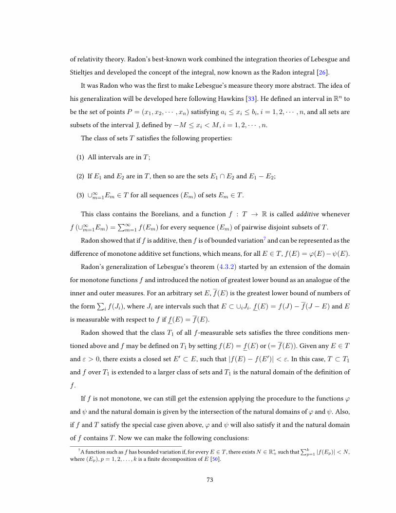
of relativity theory. Radon’s best-known work combined the integration theories of Lebesgue and

Stieltjes and developed the concept of the integral, now known as the Radon integral [26].

It was Radon who was the rst to make Lebesgue’s measure theory more abstract. The idea of

his generalization will be developed here following Hawkins [33]. He dened an interval in Rn to

be the set of points P = (x1, x2, · · · , xn) satisfying ai ≤ xi ≤ bi, i = 1, 2, · · · , n, and all sets are

subsets of the interval J, dened by −M ≤ xi < M , i = 1, 2, · · · , n.

The class of sets T satises the following properties:

(1) All intervals are in T ;

(2) If E1 and E2 are in T , then so are the sets E1 ∩ E2 and E1 − E2;

(3) ∪∞m=1Em ∈ T for all sequences (Em) of sets Em ∈ T .

This class contains the Borelians, and a function f : T → R is called additive whenever

f (∪∞m=1Em) =∑∞

m=1 f(Em) for every sequence (Em) of pairwise disjoint subsets of T .

Radon showed that if f is additive, then f is of bounded variation7 and can be represented as the

dierence of monotone additive set functions, which means, for allE ∈ T , f(E) = ϕ(E)−ψ(E).

Radon’s generalization of Lebesgue’s theorem (4.3.2) started by an extension of the domain

for monotone functions f and introduced the notion of greatest lower bound as an analogue of the

inner and outer measures. For an arbitrary set E, f(E) is the greatest lower bound of numbers of

the form∑

i f(Ji), where Ji are intervals such that E ⊂ ∪iJi. f(E) = f(J)− f(J − E) and E

is measurable with respect to f if f(E) = f(E).

Radon showed that the class T1 of all f -measurable sets satises the three conditions men-

tioned above and f may be dened on T1 by setting f(E) = f(E) or (= f(E)). Given anyE ∈ T

and ε > 0, there exists a closed set E′ ⊂ E, such that |f(E) − f(E′)| < ε. In this case, T ⊂ T1

and f over T1 is extended to a larger class of sets and T1 is the natural domain of the denition of

f .

If f is not monotone, we can still get the extension applying the procedure to the functions ϕ

and ψ and the natural domain is given by the intersection of the natural domains of ϕ and ψ. Also,

if f and T satisfy the special case given above, ϕ and ψ will also satisfy it and the natural domain

of f contains T . Now we can make the following conclusions:7A function such as f has bounded variation if, for everyE ∈ T , there existsN ∈ R∗+ such that

∑kp=1 |f(Ep)| < N,

where (Ep), p = 1, 2, . . . , k is a nite decomposition of E [50].

73

• A function F is measurable with respect to f if, for every a ∈ R, T1 contains the set P such

that F (P ) > a;

• This measurable function F is summable if the series∑∞

k=−∞ akf(Ek) converges abso-

lutely, where . . . < a−2 < a−1 < a0 < a1 < a2 < . . . is a partition of R with nite norm

and Ek denotes the set P such that ak ≤ F (P ) ≤ ak+1;

• When F is summable with respect to f ,∫J F (P )df is dened to be the limit of the above

series as the norm of the partition tends to zero.

We can compare these denitions with Lebesgue’s work, replacing m by f , and see that

Lebesgue’s work becomes a particular case of Radon’s8. In Radon, the idea of absolute continuity

is not associated with Lebesgue’s measure. Taking two additive set functions b and f , with natural

domains Tb and Tf , b is called a basis for f if b ≥ 0 and if b(E) = 0 for any set E ⊂ Tb ∩ Tf , then

f(E) = 0. When the special case applies, Tb is contained in Tf and ∀ε > 0, there exists a δ > 0,

such that |f(E)| < ε whenever b(E) < δ.

Radon was able to generalize Lebesgue’s theorem (4.3.2) to:

Theorem4.3.3. If g is an additive set function with basis f , then there exists an f -summable function

Ψ such that g(E) =∫E Ψ(P )df for every E in Tf .

This theorem by Radon if the rst part of the Radon-Nikodyn theormem, as we will show

in this chapter, and is an important step to generalize the notions of conditional probability and

conditional expectation as we will discuss in chapter 5.

4.3.6 Carathéodory’s axioms for measure theory

Constantin Carathéodory was born in Berlin, in 1873, and died in Munich, in 1950. From

1891 to 1895, he attended the École Militaire de Belgique. After completing his education, he went

to Egypt in the employ of the British government as an assistant engineer. In 1900, however,

Carathéodory decided to go to Berlin to study mathematics. Carathéodory gave contributions in

the calculus of variations, in the theory of functions and, in what is our main interest here, the

theory of real functions, of the measure of point sets and of the integral. Carathéodory’s book on8Radon’s work also generalizes the Stieltjes’ integral. Although we will not discuss it here, as it is not the focus of

this thesis, the interested reader can nd an exposition of the Stieltjes integral in [59], and of Radon’s generalization in[33].

74

this subject represents both a completion of the development begun by Borel and Lebesgue and

the beginning of the modern axiomatization of this eld [26].

Carathéodory introduced the concept of outer measure in Rn using ve axioms presented in

[34]:

(1) The function µ∗ associates to any part of Rq a value in R+;

(2) If B ⊂ A ⊂ Rq , then µ∗(B) ≤ µ∗(A);

(3) If (An) ⊂ Rq is a nite or countable sequence of sets, µ∗(∪nAn) ≤∑

n µ∗(An). A set A

is measurable if it satises the Carathéodory condition, that is, for any set W , we have:

µ∗(W ) = µ∗(W ∩A) + µ∗(W ∩Ac);

(4) If A1, A2 ⊂ Rq and infd(x, y) : x ∈ A1, y ∈ A2 > 0, where d is the Euclidian distance

in Rq , so µ∗(A1 ∪A2) = µ∗(A1) + µ∗(A2);

(5) The outer measure of a setA is the lim inf µ∗(B), whereB is a collection of measurable sets

containing A. The inner measure of A is given by: µ∗(A) = µ∗(A)− µ∗(B\A).

In coming up with this axiomatization of the outer measure, Caratheodory proved an impor-

tant theorem that carries his name and provides us a way to extend a measure on an algebra of sets

to a measure on a σ-algebra. The set of all measurable sets forms a σ-algebra and the outer mea-

sure µ∗, restricted to the set of measurable sets is a measure. Carathéodory’s extension theorem

is stated in many dierent ways, but we’ve chosen the version in Bartle [5]:

Theorem 4.3.4 (Carathéodory extension theorem). The collection A∗ of all µ∗-measurable sets is

a σ-algebra containing the algebra A. Moreover, if (En) is a disjoint sequence of sets in A∗, then

µ∗(∪∞n=1En) =∞∑n=1

µ∗(En).

The idea of this theorem is that, if A is any algebra of subsets of a set X and if µ is a measure

dened on A, then there exists a σ-algebra A∗ containing A and an outer measure µ∗ dened on

A∗ such that µ∗(E) = µ(E) for all E in A. So the measure µ can be extended to a measure on a

σ-algebraA∗ of subsets of X that containsA. In addition, if the measure is σ-nite, the extension

is unique. This result is called the Hann extension theorem and the interested reader can consult

75

[4] or [53] for a complete exposition. Carathéodory’s extension theorem is one of the key results

in measure theory that aorded the construction of the axioms. With this extension theorem,

Kolmogorov was able to take a measure dened on an algebra of sets and extend it to a σ-algebra

generated by this algebra. This was a great result that allowed Kolgomorov create the axiom that

takes probability out of the nite scope of the classical approach to innite probability spaces.

4.3.7 Fréchet’s integral on non-Euclidian spaces

Maurice Fréchet was born in Maligny, France, in 1878, and died in Paris, in 1973. At the Lycée

Buon in Paris, Frechet was taught mathematics by Jacques Hadamard, who perceived his pupil’s

precocity. Fréchet entered the École Normale Supérieure in 1900, graduating in 1903. He wrote up

the lectures of Émile Borel that were turned into a book. This work was part of a long and close

relationship between Borel and Fréchet that continued as long as Borel lived.

From 1907 to 1910, Fréchet held teaching positions at lycées in Besançon and Nantes and at

the University of Rennes. He held a professorship at Poitiers, but was on leave in military service

throughout World War I, mainly as an interpreter with the British army. From 1919 to 1928, he

was head of the Institute of Mathematics at the University of Strasbourg.

Fréchet made many contributions to topology, developing the concept of metric space, com-

pactness, separability, and completeness. He established the connection between compactness and

what later came to be known as total boundedness. He came up with a great number of gener-

alizations in topology and in Euclidian spaces and probability. Among his results, we are mainly

interested in here is the formulation of an important generalization of the work of Radon, showing

how to extend the work of Lebesgue and Radon to the integration of real functions on an abstract

set without a topology, using merely a generalized measurelike set function [26].

Fréchet was able to take Radon’s integral and raise it to a higher level of abstraction. In his

work of 1959 [24], he stated Radon’s integral∫F (P )dh(P ), where F (P ) is a function of a point

P of an n-dimensional space, and h(P ) is a function of limited variation. He then proposes to

state Radon’s integral as∫E F (P )df(e), where f(e) is an additive function of the variable subset

e ⊂ E and E is an abstract set. In Fréchet’s words, ... la dénition et les propriétés de l’intégrale

de M. Radon s’étendent bien au delà du Calcul intégral classique, elles sont presque immédiatement

applicable au domaine inniment plus vaste du calcul fonctionnel (p. 249). Fréchet had mentioned

that in order to get this generalization, we can preserve most of Radon’s denition and neglect the

76

nature of P , that is, a point in the n-dimensional space. By doing so, we can get an integral in the

more general scope of the functional calculus.

Fréchet denes an abstract set as one that we don’t know the nature of its elements, that is,

this nature doesn’t interfere in our reasoning regarding this set. He follows with other denitions

such as a family of additive sets, a set function, total variation and limit of a sequence of sets

to enter the integration of an abstract functional. He denes the upper and lower integral of a

bounded functional and states that it is integrable if its upper and lower integral coincide. He then

extends this integration to unbounded functionals, exposes some properties of this new integral

and nishes with a section on measurable functionals.

As acknowledged by Kolmolgorov, Fréchet’s integral opened paths to achieve a general and

abstract axiomatization of probability. In the preface, Kolmogorov writes: After Lebesgue’s investi-

gations, the analogy between the measure of a set and the probability of an event, as well as between

the integral of a function and the mathematical expectation of a random variable, was clear. This

analogy could be extended further; for example, many properties of independent random variables

are completely analogous to corresponding properties of orthogonal functions. But in order to base

probability theory on this analogy, one still needed to liberate the theory of measure and integration

from the geometric elements still in the foreground with Lebesgue. This liberation was accomplished

by Fréchet [39] (p. v).

4.3.8 The Radon-Nikodym theorem

Although Lebesgue’s integral became more general with Fréchet, who extended it to non-

Euclidean spaces, the complete abstraction was accomplished by Nikodym, giving the theorem

known as the Radon-Nikodym theorem. This theorem is in the heart of the modern denitions of

conditional probability and conditional expectation with regards to a σ-algebra as we will show in

the next chapter. In order to describe this theorem, we introduce three important denitions from

[5] and [53]:

If there exists a sequence (En) of sets in theσ-algebra andX = ∪En and such thatµ(En) <∞

for all n, then we say that µ is σ-nite.

For example, the Lebesgue measure on R with the Borelian σ-algebra is not nite, but it is

σ-nite. As another example, let N be the set of natural numbers andA be the σ-algebra of all the

subsets of N. If E is any subset of N, dene µ(E) to be the number of elements of E if E is nite

77

and equal to +∞ if E is innite. Note that µ is a measure and is called the counting measure on

N. µ is not nite, but it is σ-nite.

To exemplify a measure that is not σ-nite, think ofX as a non-empty set andA the σ-algebra

of all subsets of X . Let’s dene µ(∅) = 0 and µ(E) = +∞ if E 6= ∅.

A proposition holds µ-almost everywhere if there exists a subset N in the σ-algebra with

µ(N) = 0 such that the proposition holds on the complement of N . In this denition, we can

say that the proposition holds for every element of the set we are analyzing, except in a subset of

measure zero.

A measure λ is absolutely continuous to the measure µ in the sense that, if E is in the σ-algebra

and µ(E) = 0, then λ(E) = 0.

As an example of absolute continuity between two measures, let X be the interval [0, 1], and

B the borelian σ-algebra on X . Dene µ as the Lebesgue measure on X and let λ assign twice the

length of each subset Y of X . Note that λ is absolutely continuous with respect to µ.

Now, let X and µ be dened as in the example above and let ν assign to each subset Y of

X , the number of points from the set 0.1, ..., 0.9 that are contained in Y . Note that ν is not

absolutely continuous with respect to µ, because ν assigns non-zero measure to zero-length sets

such as Q ∩ [0, 1].

Once the concepts above are dened and exemplied, we enunciate:

Theorem 4.3.5 (Radon-Nikodym). Let µ and ν be σ-nite measures on the σ-algebra A and ν is

absolutely continuous with respect to µ. Then there is a function f ≥ 0 such that

ν(E) =

∫Efdµ, E ∈ A.

Moreover, f = dνdµ is called the Radon-Nikodym derivative and it is uniquely determined µ-almost

everywhere.

To develop an intuition as to what this theorem says, we can think in terms of probability

measure. Let’s set P (A) =∫A f(x)dx. With the Radon-Nikodym theorem, we can represent the

probability of the set A, P (A), as the density function f(x). The Radon-Nikodym derivative of

P (A) is then the density function f(x).

Even though this example can be useful to develop an intuition into the Radon-Nikodym

78

derivative, we should keep in mind that this theorem is general and applies to arbitrary mea-

sures, beyond the scope of probability or Lebesgue measures. It is also valid for arbitrary spaces

beyond the Euclidean one.

Now that we have presented the essential results from measure theory that were necessary

to build modern probability in a general and abstract context, the next section will present the

evolution of the works of mathematicians that tried to connect probability with measure theory

or build the theory of probability in a way that would overcome the limitations of the classical

approach.

4.4 The search for the axioms and early connections betweenprob-

ability and measure theory.

In this section we expose the evolution of the ideas in probability from its association to mea-

sure theory up to the preliminary foundation required for the construction of the axioms. We will

begin the exposition by the association of probability and measure as given by Hausdor and the

call for axiomatization by Hilbert. After that, we will present an essential contribution made by

Borel’s work on denumerable probability, where he introduced countable additivity to probability,

introduced the result of the strong law of large numbers and connected binary experiments, like

heads and tails, to an uncountable set. Finally, we will present the rst attempts at axiomatization

and the evolution of probability towards a more abstract context.

4.4.1 The connection of measure and probability and the call for the axioms

The association of probability and measure theory was well established with the work of Felix

Hausdor. Although some association between the two had been previously explored by other

authors, in Hausdor’s work, he takes probability as an application of measure theory and gives a

rigorous treatment to Poincaré’s intuition that probability 0 doesn’t necessarily mean impossibility

and asserted that many "theorems on the measure of point sets take on a more familiar appearance

when expressed in the language of probability calculus" [67] (p. 35).

Hausdor stated that the measure normalized is dened to be a probability. Today we take

the opposite approach, that is, probability is dened formally as a measure. Hausdor’s book was

considered the standard reference for set theory, and we will consider the connection between

79

probability and measure theory established in his work of 1914.

At the beginning of the 20th century, classical probability was showing its limits, and mathe-

maticians were searching for a rigorous denition that would formally dene terms such as event,

trial, randomness and even probability itself. Poincaré says: "On ne peut guère donner une dénition

satisfaisante de la Probabilité. On dit ordinairement : la probabilité d’un événement est le rapport du

nombre des cas favourables à cet événement au nombre total des cas possibles [51] (p. 24)".

Hilbert’s well known list of open problems in mathematics, published in the International

Congress of Mathematicians in Paris in 1900, called for an axiomatization of those parts of physics

in which mathematics played an important role, with a special attention to probability and me-

chanics. Hilbert was concerned about the foundations of statistical mechanics. He was searching

for a rm mathematical basis for the determination of average values, that could be found using

probability distributions for the quantity considered [67]. In a survey on the works of history from

measure to probability, Bingham points to Hilbert’s description of probability as a physical science

in his call for the axioms as evidence as to the unsatisfactory state of probability. In his own words:

Hilbert’s description of probability as a physical science, which one can hardly imagine beingmade

today, is striking, and presumably reects both the progress in statistical mechanics byMaxwell, Boltz-

mann and Gibbs and the unsatisfactory state of probability theory at that time judged as mathematics

[9] (p. 146).

4.4.2 Borel’s denumerable probability

Borel made substantial contribution to probability in his 1909 paper: Les probabilités dénom-

brables et leurs applications arithmétiques. In this paper, he employs the use of countable additivity

to probability and also develops an astonishing result: the strong law of large numbers. Borel

starts his text saying that there are two categories in probability problems, when the number of

possible cases is nite and the continuous probability. He then introduces a new category, the one

of the countable sets, which is placed between the nite and the continuous probabilities.

In this same work, Borel takes a number x ∈ [0, 1] and represents it with binary digits (0’s and

1’s). Setting, x = b1b2 · · · and [0, 1] with the Lebesgue measure, Borel shows that x = b1b2 · · ·

becomes a random variables with the same distribution used in calculating the probability of the

outcome of successive and independent coin tosses. He says that the probability assigned to the

event that the n tosses of a coin gives one specic sequence of heads and tails is 2−n. This value is

80

also the Lebesgue measure of the nite set of intervals whose points x have binary representations

with a specied sequence of 0’s and 1’s in the rst n places.

Borel explains the importance that he gives to the countable sets in probability. In his own

words: ... cette notion du continu, considéré comme ayant une puissance supérieure à celle du dénom-

brable, me paraît être une notion purement négative, la puissance des ensembles dénombrables étant

la seule qui nous soit connue d’une manière positive, la seule qui intervienne eectivement dans nos

raisonnements. Il est clair, en eet, que l’ensemble des éléments analytiques susceptibles d’être réelle-

ment dénis et considérés ne peut être qu’un ensemble dénombrable; je crois que ce point de vue

s’imposera chaque jour d’avantage aux mathématiciens et que le continu n’aura été qu’un instru-

ment transitoire, dont l’utilité actuelle n’est pas négligeable (...), mais qui devra être regardé seulement

comme un moyen d’étudier les ensembles dénombrables, lesquels constituent la seule réalité que nous

puissions atteindre [13] (p. 247-248).

Three possible cases of denumerable probabilities are distinguished:

(1) A limited number of possible outcomes in each try, but with a countably innite number of

tries;

(2) Countably innitely many possible cases in each try, but the number of tries is nite;

(3) The possible cases and the number of tries are both countably innite.

Borel mentions that he starts by the rst case (countable innite many tries of a nite number

of possible outcomes) and begins to present many probability problems. We explain the rst three

problems, which are the relevant ones for the proof of Borel’s strong law of large numbers.

• Problem 1: What’s the probability that the favourable cases never happen?

Borel denotes pn the probability of success in the nth trial, and A0 the probability of the event

that a favourable case will never occur, whereA0 is given by: A0 = (1−p1)(1−p2) · · · (1−pn) · · · .

He excludes any case in which pn = 1 and then concludes that if

∞∑n=1

pn (3)

is convergent, then 0 < A0 < 1. In case of divergence of the series (3), A0 = limn→∞∏ni=1(1 −

pi) = 0, so A0 goes to zero as n grows. In this case, Borel takes some caution in his explanation,

81

recalling that probability zero doesn’t necessarily mean impossibility. He recalls his paper of 1905

[12] where he explains that the probability of choosing a rational number at random is zero, but

it doesn’t mean that there are no rational numbers. Having noted this, Borel concludes that in the

case of divergence,A0 = 0, but it only means that the probability that no favorable case will occur

goes to zero when the number of trials increases indenitely.

• Problem 2: What’s the probability that the favourable cases happen exactly k times?

Borel denotes this probability Ak and starts analyzing the case where k = 1.

If the favourable case happens in the rst trial we have: ω1 = p1(1−p2)(1−p3) · · · (1−pn) · · · .

If the series (3) is convergent, then ω1 = p11−p1A0. If the series is divergent, ω1 = 0.

He then presents the case of the favourable case happening in the nth trial as ωn = pn1−pnA0.

A1 will be the sum of all the ωn and we get: A1 = A0

(p1

1−p1 + p21−p2 + · · ·+ pn

1−pn + · · ·)

.

The series inside the parenthesis is convergent, and Borel sets: un = pn1−pn = pn

qnand A1 =

A0∑∞

i=1 un.

In case of divergence of the series (3), we also have divergence in the sum of the un’s and

A0 = 0. In this case, A1 is indeterminate, of the form 0 · ∞. If we see that A1 is the sum of

the ωn’s, and that each ωn is zero in the divergent case, we have that A1 is a countable sum of

zeros, so it should be zero. Borel doesn’t feel comfortable using this fact, saying that even if the

ω’s are all zero, there are innitely many of them, so we can’t conclude without caution that their

sum is zero, if we keep in mind that zero probability doesn’t necessarily mean impossibility. So he

develops an argument and nally concludes the result that A1 = 0 in the divergent case.

After this, he gives the result that Ak = A0∑un1un2 . . . unk

if (3) is convergent and Ak = 0

if the series is divergent.

• Problem 3: What’s the probability that the favourable cases happen an innite number of

times?

Borel starts by denotingA∞, the probability of favourable cases happening an innite number

of times. He then considers the case where (3) is convergent and evaluates the sum: S = A0+A1+

· · ·+Ak + · · · . He says that by the previous results on the Ak we can write: S = A0(1 +u1)(1 +

u2) · · · (1 + uk) · · · . Now using the fact that A0 = (1 − p1)(1 − p2) · · · (1 − pn) · · · and un =

pn1−pn = pn

qn, we have that 1 = un = 1

1−pn . Taking the product, we get∏

(1+un) =∏ 1

1−pn = 1A0

82

and we can nally write: S = A01A0

= 1. To conclude, A∞ is exactly the complement of S, so

A∞ = 1− S = 0.

In the case of divergence of the series (3), each Ak = 0, so S = 0 and A∞ = 1, however Borel

again develops an argument to show this result because he wasn’t comfortable with summing

zeros a countable innite number of times.

With the three problems presented here, we have demonstrated the following result:

Theorem4.4.1 (Borel 0-1 law). Let’s take a countable innite sequence of independent binary events,

where pn is the probability of a favorable case occurring in the nth trial.

If∑∞

n=1 pn <∞, then A∞ = 0.

If∑∞

n=1 pn =∞, then A∞ = 1.

A few years later, Cantelli remarked that the hypothesis of independence of the Borel 0-1 law

could be relaxed and this new result is known as the Borel-Cantelli lemma.

Borel applies his 0-1 law with the dyadic expansion of a real number x chosen at random in

[0, 1] and he developed an astonishing result, the strong law of large numbers, which we will now

present.

Any x ∈ [0, 1] can be written as: x = ·b1b2 . . . bn . . . =∑∞

n=1bn2n , where each bn is either 0 or

1. When the sequence (bn) is generated, or equivalently x is chosen, each digit bn has probability

1/2 of being 0 or 1 and the digits n = 1, 2, . . . are independent trials [4].

Borel adopted 0 as the favourable case and stated that if we take 2n trials, the probability that

the number of favourable cases will be between

n− λ√n and n+ λ

√n

is given by

Θ(λ) =2√π

∫ λ

0e−λ

2dλ

and this probability converges to 1 as λ increases.

Borel takes a sequence (λn), with λn = log n, so (λn) is an increasing sequence such that

limn→∞λn√n

= 0.

The rst 2n trials give a favourable result if the number of times that 0 appears will be between

n− λn√n and n+ λn

√n.

83

The probability pn of the favourable case is:

pn = Θ(λn) =2√π

∫ λn

0e−λ

2dλ.

Now Borel sets qn = 1 − pn. The sum of qn is convergent, so the probability of having

non-favourable cases innitely many times is 0. He concluded that, after a certain value n, the

probability of constantly being in the favourable case is 1. The ratio between the number of 0’s

and the number of 1’s will be between:

n− λn√n

n+ λn√n

and n+ λn√n

n− λn√n, or equivalently between 1− λn/

√n

1 + λn/√n

and 1 + λn/√n

1− λn/√n.

One big aw of Borel’s proof here is that he assumes the convergence of the pn’s according

to the Central Limit Theorem, however the classic version of that theorem considers independent

and identically distributed random variables, which is not the case because λn is not xed [4].

Also, as pointed out in [67], the convergence of the∑qn =

∑(1− pn) is not guaranteed by the

convergence of the series of the Θ(λn).

Even though the proof of Borel’s strong law is not perfect, the authors that came after him

were able to x it, as will be seen in the last section of this chapter. But a question that arises and

needs to be raised at this point is: What is the innovation of this result? What is the dierence

between the weak and the strong law of large numbers?

To answer these questions, let’s denote by ν2n(x) the number of 0’s in the rst 2n trials of a bi-

nary experiment. While the weak law, in today’s version, states that limn→∞ P(∣∣∣ν2n(x)

2n − 12

∣∣∣ > ε)

=

0, the strong law states that P(

limn→∞ν2n(x)

2n = 12

)= 1.

This means that the weak law states a probable proximity, but doesn’t guarantee a convergence

for the relative frequency. That is, with a suciently large sample, there will be a very high

probability that the average of the observations will be within an arbitrarily small interval around

the expected value, but it is still possible that |Xn − µ| > ε happens an innite number of times,

although at infrequent intervals.

The strong law doesn’t leave room for this possibility to happen, because it says that there is

a probability 1 that the limit always applies, that is, for any ε > 0 the inequality |Xn − µ| < ε

holds for all n large enough.

84

4.4.3 The rst attempts at axiomatization

An early attempt at axiomatization came from Laemmel in 1904. He had worked on the inde-

pendent case and discussed the rules of total and compound probability as axioms, but didn’t give

any explanation of the concept of independence [56].

Ugo Broggi’s dissertation under Hilbert’s direction in 1907, proposed two axioms: i) the certain

event has probability 1, and ii) the rule of total probability. After these axioms, he dened proba-

bility as a ratio of the number of cases for a discrete set, and the ratio of the Lebesgue measures in

the geometric setting. To Broggi, total probability implied countable additivity, which would later

be contested by Steinhaus. This last one mentions the generalization of Lebesgue’s measure for all

the subsets E of the interval [0, 1] given by Banach, that shows the existence of a function µ(E)

which is nite additive but not countably additive[63].

From 1918 to 1920, Daniell developed the integral of a linear operator on some class of con-

tinuous real-valued functions on an abstract set E. Applying Lebesgue’s methods in this general

setting, Daniell extended the linear operator to the class of summable functions. Using ideas from

Fréchet, Daniell also gave examples in innite-dimensional spaces and used his theory of integra-

tion to construct a theory of Brownian motion.

In November 1919, Wiener submitted an article where he laid out a general method for setting

up Daniell’s integral when the underlying space E is a function space. Daniell was aware of the

importance of Brownian motion and of its model in physics made by Einstein. He then followed

with a series of articles where he used Daniell’s integral to formalize the notion of Brownian

motion on a nite time interval.

In 1923, Antoni Lomnicki published an article where he proposed that probability should be

faced relative to a density φ on a setM in Rn. He had used two ideas from Carathéodory: the

rst one was that of a p-dimensional measure and the second one was that of dening the integral

of a function on a set as the measure of the region between the set and the function’s graph. To

Lomnicki, the probability of a subset m ⊂M is the ratio of the measure of two regions: that one

between m and φ’s graph and that between M and this graph. Together with Ulam, Lomnicki

was the rst to take probability outside the geometric context and lead it to abstract spaces. Ulam,

at the 1932 International Congress of Mathematicians in Zurich, announced that Lomnicki had

shown that product measures9 can be constructed in abstract spaces. Ulam asserted that their9If (X,A, µ) and (Y,B, ν) are measure spaces, then there is a measure π, called the product measure, dened on the

85

probability measure satises the same conditions on the product space of a countable sequence of

spaces. Their idea can be put in today’s language as: m is a probability measure on a σ-algebra

that is complete10, that is, includes all null sets, and contains all singletons. Ulam and Lomnicki’s

axioms were published in 1934 citing Kolmogorov’s Grundbegrie as an authority to their work.

Von Mises was a mathematician concerned with applied studies who aimed to create a statis-

tical physics freed from mechanical assumptions. In his point of view, classical mechanics cannot

serve as a foundation for statistical physics and a genuine probabilistic behaviour is not compat-

ible with a mechanical description. After this point of view, he made signicant contributions in

formulating a system for statistical physics based on the use of Markov chains.

He has his name associated with the frequentist approach in probability, and was pointed by

some authors as "a crank semimathematical theory serving as a warning of the state of probability be-

fore the measure theoretic revolution" [67] (p. 180). What is striking in this story is that Kolmogorov

himself based the application of probability on von Mises’ ideas, as he explains in a foot-note of

the Grundbegrie: The reader who is interested in the purely mathematical development of the the-

ory only, need not read this section, since the work following it is based only upon the axioms in §1

and makes no use of the present discussion. Here we limit ourselves to a simple explanation of how

the axioms of the theory of probability arose and disregard the deep philosophical dissertations on

the concept of probability in the experimental world. In establishing the premises necessary for the

applicability of the theory of probability to the world of actual events, the author has used, in large

measure, the work of R. v. Mises. [39] (p. 3).

Von Mises published a work in 1919 concerned with the foundations of probability, where he

proposed a foundational system. This system was based on a sample space of possible results, each

represented by a number, with an experiment that is repeated indenitely. The resulting sequence

of numbers is called a collective if: i) the limits of relative frequencies in that sequence exist and

ii) these limits remain the same in subsequences formed of original sequence. From the denition

of collectives, probability is dened as the limit of relative frequency, with the second item giving

us the postulate of randomness.

As one of the founders of logical empiricism, von Mises considered mathematical innity an

idealization that could not claim empirical reality directly, but only as a useful tool. One of the most

subsets of Z = A× B such that π(A×B) = µ(A)ν(B) for all A ∈ A and B ∈ B [53].10A measure space (X,M, µ) is said to be complete providedM contains all subsets of sets of measure zero, that is,

if E belongs toM, and µ(E) = 0, then every subset of E also belongs toM [53].

86

important critiques of von Mise’s collectives came from Jean Ville [66]. Regarding the randomness

postulate, one may ask if a property appears as truly randomly distributed in a population or if a

dierent frequency of the outcomes could be obtained by a more informed way of sampling. This

critique can be associated with the result of a sequence of 0’s and 1’s. If the limit of a sequence of

relative frequencies is neither 0 nor 1, then it can be dierent from a subsequence composed by

only 0’s or only 1’s.

Ville’s strongest objection to von Mise’s collectives is that this theory is not compatible with

countable additivity. His argument relys on the limit theorems, where convergence occurs in-

nitely often. Ville stated that there is a collective such that the frequency of 1’s in the sequence

is always greater than or equal to p. In this same work, Ville creates the important concept in

probability of Martingale.

In 1922, a paper written by the Soviet mathematician Eugen Slutsky provided a new approach

to the development of probability theory, which he devised while trying to answer Hilbert’s 6th

problem. In his attempt to make probability purely mathematical, he removed the word probabil-

ity and the idea of equally likely cases from the theory. This was the rst time that probability

theory did not depend on equally likely cases. According to Slutsky, to develop this theory, instead

of bringing up equally likely cases, one should start by just assuming that numbers are assigned

to cases, and when a case that has been assigned with the number α is divided in sub-cases, the

sum of the numbers of the sub-cases should add to α. It is not required that each case has the same

number. Slutsky proposed something very general that he called "valence", with three possible

interpretations: i) classical probability, based on equally likely cases, ii) nite empirical sequences

and iii) limits of relative frequencies. So it can be said that probability would be one possible inter-

pretation for Slutsky’s valences. To Slutsky, probability could not be reduced to limiting frequency,

as the latter has very limiting properties to the former.

In the year following the publishing of Slutsky’s paper, Steinhaus [63] proposed a set of axioms

to Borel’s theory of denumerable probability. He dened:

• A as the set of all possible innite sequences of heads and tails (H and T);

• E,E′, . . . as subsets of A;

• En as subsets of A with rst n elements in common, n = 0, 1, 2, . . . or∞;

• M as a class of all subsets of A and

87

• K as a class of certain subsets of E, that is, the class K is part of M.

Then he sets µ to be a set function dened for all E ∈ K such that:

(1) µ(E) ≥ 0 for all E ∈ K;

(2) (a) µ(A) = 1;

(b) En ∈ K;

(c) If two sets En and E′n only dier in the ith element, (i ≥ n), then µ(En) = µ(E′n);

(3) K is closed under nite and countable unions of disjoint elements, and µ is nitely and

countably additive.

(4) If E2 ⊂ E1, and E1 and E2 are in K, then E1\E2 is in K.

(5) If E is in K and µ(E) = 0, then any subset of E is in K.

Steinhaus concluded that the theory of probability for an innite sequence of binary trials is

isomorphic to the theory of Lebesgue measure. Although Steinhaus considered only binary trials,

his reference to Borel’s more general concept of denumerable probability opened paths to further

generalizations [56].

Kolmogorov himself made signicant contributions to probability theory before publishing

his axioms. In 1925’s article with Khinchin [38] Kolmogorov proved the convergence, with prob-

ability 1, of a series of random variables and also gave the sucient and necessary conditions

for that convergence. In 1928, Kolmogorov wrote an article [37] where he proved what he called

the generalized law of large numbers, which is a version of the strong law for independent ran-

dom variables. Kolmogorov’s article of 1929 [35] denes several probability ideas using measure

theory. He expresses his concerns with the possibility of constructing a very general and purely

mathematical theory to solve probability problems. In this article he considered a set A endowed

with a measure M , (A,M) is a metric space, and some subsets E ⊂ A. Then he dened three

axioms for his measure: i) M(E) ≥ 0; ii) if E1 ∩E2 = ∅, then M(E1 ∪E2) = M(E1) +M(E2),

and; iii) M(A) = 1. From these axioms, he showed some standard results in probability but what

calls attention in this work is the use of countable additivity. He dened a normal measure as

one where countable additivity holds. This concept necessary to justify arguments involving the

88

convergence of random variables. In his work of 1931 [36], on continuous time stochastic process,

Kolmogorov freely uses countable additivity and also Fréchet’s framework for abstract sets.

Cantelli constructed a theory with no appeal to empirical notions, such as possibility, event,

probability or independence. His theory started with an abstract set of points with positive and

nite measure. We can enumerate his denition from [56]:

(1) m(E) is the area of a subset E;

(2) m(E1 ∩ E2) = m(E1) +m(E2) when E1 and E2 are disjoint;

(3) 0 ≤ m(E1E2)/m(Ei) ≤ 1, for i = 1, 2.

(4) E1 and E2 are called multipliable when m(E1E2) = m(E1)m(E2).

Even though Cantelli’s work was general and abstract, Kolmogorov’s works of 1929 and 1931

had already gone beyond Cantelli’s contributions in abstraction and mathematical clarity. How-

ever, it’s important to note that Cantelli had developed, independently of Kolmogorov, the combi-

nation of a frequentist interpretation of probability with an abstract axiomatization that incorpo-

rated classical rules of total and compound probability [56].

4.4.4 The proofs of the strong law of large numbers

Borel’s strong law of large number was a quite surprising result: the measure of binary dec-

imals with a limiting frequency of 1’s dierent from 1/2, is zero. Following, Borel’s result, many

mathematicians started to work on the strong law of large numbers to improve its results. Faber

constructed a continuous function f where the set of points x where f doesn’t have a derivative

has Lebesgue measure 0. Letting n(1) and n(0) denote the numbers of 1’s and 0’s, respectively, in

the rst n binary digits of x, if lim inf(n(1)/n(0)) < 1 − ε or lim sup(n(1)/n(0)) > 1 + ε, then

there is no derivative. It follows that the set of x for which lim(n(1)/n(0)) = 1 has measure 1

[56].

Hausdor also proves Borel’s strong law of large numbers. Putting n(1) as above, Hausdor

shows that n(1)/n→ 1/2 as n→∞, except on a set of measure 0. He then studies the asymptotic

behavior of the oscillation of frequency. Hausdor found limits of ± log n√n for the deviation of

the number n(1) from the average n/2 [56].

89

Hardy and Littlewood [31] (p. 185) have shown that, with n(1) as above, |n(1)−n/2|√n logn

→ 1 as

n → ∞, except for on a set of measure 0. They point out that√n log n is an upper bound for

the deviation of the frequency |n(1) − n/2| and that√n can be improved as a bound, because

lim inf |n(1)− n/2| >√n (p. 187).

In 1923, Khintchin improved Hardy and Littlewood’s upper bound to√n log log n. This result

is known as the law of iterated logarithm and one year later he was able to show that this bound

cannot be improved. Khintchin considered a simple event with probability of success p and has

shown that there is a functionχ(n) such that for any ε and δ, there is a natural numbern0 such that,

with a probability greater than 1− δ we have, for all n > n0, the inequality: 1− ε <∣∣∣n(1)−n/2

χ(n)

∣∣∣ <1 + ε. The solution gives with q = 1− p the asymptotic expression:

√2pqn log log n.

Maistrov [46] presents Khintchin’s idea geometrically. In Figure (4.6), the values ofn are placed

on the x-axis and the values of n(1) − n/2 on the y-axis. Then two straight lines, y = εn and

y = −εn, are drawn. By the Borel-Cantelli lemma, for n large enough, the value n(1)− n/2 will

almost certainly stay between the lines y = εn and y = −εn. What Khintchin had accomplished

to do was to nd that for any ε and n large enough, the quantity n(1) − n/2 will stay with near

certainly within the curves:

• y = (1 + ε)(2npq log log n)1/2 (l)

• y = −(1 + ε)(2npq log log n)1/2 (l’)

and outside the curves

• y = (1− ε)(2npq log log n)1/2 (ll)

• y = −(1− ε)(2npq log log n)1/2 (ll’)

innitely often.

Khintchin was able to show that if the probability of occurence of the event A in each of the

n independent trials is equal to p, then the number n(1) of occurrences of the event A in n trials

satises:

P

(lim supn→∞

n(1)− n/2(2npq log log n)1/2

= 1

)= 1.

In 1928, Khintchin showed that if a sequence of random variables were independent and iden-

tically distributed, the existence of the expectation was a necessary and sucient condition to

90

Figure 4.6: Khintchin’s bounds - [46] (p. 260).

apply the weak law of large numbers. Kolmogorov discovered the conditions to be imposed on a

sequence of random variables in order for the strong law of large numbers to hold, which in the

case of independent and identically distributed random variables, is the existence of expectation.

In all of these investigations, the analogy with metric theory of functions played a signicant

role, and Kolmogorov started to engage in the logical formulation of these ideas which ended in

the formulations of the axioms of probability that we describe in the next chapter.

91

Chapter 5

Kolmogorov’s foundation of

probability

5.1 Introduction

Andrei Nikolaevich Kolmogorov was born in Tambov, Russia, in 1903, and died in Moscow,

in 1987. Kolmogorov had wide-ranging intellectual interests, including Russian history and Alek-

sandr Pushkin’s poetry. Kolmogorov entered Moscow University in 1920 to study mathematics.

Following his graduation in 1925 and his doctorate four years later, he became a professor at

Moscow University’s Institute of Mathematics and Mechanics in 1931. Kolmogorov taught math-

ematically gifted children for many years and served as the director for almost seventy advanced

research students, many of whom became signicant mathematicians in their own right. He is

considered one of the 20th century’s greatest mathematicians, with a rarely found level of creativ-

ity and versatility. Besides probability, Kolmogorov also made contributions to many other elds,

such as algorithmic information theory, the theory of turbulent ow, dynamical systems, ergodic

theory, Fourier series, and intuitionistic logic [26].

In his book Foundations of the Theory of Probability, Kolmogorov was able to identify the con-

tributions from many authors, including himself, and summarize those ndings in such a powerful

way that the work of those who came before him became overshadowed by the synthesis that he

did. Kolmogorov developed the subject in a fully abstract way, beyond Euclidean spaces, and for-

malized terms that had previously been only loosely dened (such as event, random variable and

92

even probability). This ability to capture the most essential ideas and create a set of abstract axioms

put an end to classical probability and started the era of modern probability when this discipline

became an autonomous branch of mathematics.

In the preface, Kolmogorov says that the purpose of his book is to give an axiomatic foundation

for probability. As he said: "the author set himself the task of putting in their natural place, among

the general notions of modern mathematics, the basic concepts of probability theory" (p. v). Be-

sides the historical exposition of the evolution of probability before Kolmogorov’s book presented

in chapter four, his own words establish the purpose of his work as one of synthesis. "While a

conception of probability theory based on the above general viewpoints has been current for some

time among certain mathematicians, there was lacking a complete exposition of the whole system,

free of extraneous complications" (p. v). Nonetheless, his book also makes some advances and in-

novations to science. Besides the axioms, Kolmogorov also exposes other original contributions

such as probability distributions in innite-dimensional spaces (Chapter III, §4), which provided

a framework for the theory of stochastic processes; dierentiation and integration of mathemat-

ical expectations with respect to a parameter (Chapter IV, §5); a general treatment of conditional

probabilities and expectations (Chapter V), built on Radon-Nikodyn’s theorem. As Kolmogorov

mentions: "It should be emphasized that these new problems arose, of necessity, from some perfectly

concrete physical problems" (p. v).

Kolmogorov’s book, constructs the axiomatization in two chapters. In the rst one, he presents

ve axioms considering a nite sample space. The main contribution there is the set of axioms

that formalized and generalized the classical denition in nite spaces. The second chapter adds

another innovation to the denition, because it reaches its full generality when Kolmogorov intro-

duces axiom VI and takes probability to innite spaces. After this introduction, in the next section,

we present the denitions of probability from Kolmogorov’s book and demonstrate in more de-

tail some theorems that he gave an abbreviated proof. The third section presents the concepts

of probability functions, random variables and conditional probability according to Kolmogorov’s

developments, and we present conditional mathematical expectation following modern textbooks.

In the last section, we illustrate how Kolmogorov’s work has established the grounds for proba-

bility theory free of ambiguities. In order to do so, we present an example that leads to a paradox

in classical probability which is resolved by Kolmogorov’s new approach using conditional prob-

ability.

93

5.2 Kolmogorov’s axioms of probability

5.2.1 Elementary theory of probability

Kolmogorov’s denition of probability is given in the rst two chapters of his book. The rst

one is restricted to what he called elementary theory of probability, which is set up in nite sample

spaces. In the second chapter he introduces another axiom that enables us to work with innite

probability spaces.

Figure (5.1)1 presents Kolmogorov’s axioms I through V from the rst chapter of his book.

Figure 5.1: Kolmogorov’s axioms I to V - [39] (p. 2).

After presenting the axioms, Kolmogorov presents a brief discussion on how to construct

elds of probability. He takes a nite set E = ξ1, ξ2, . . . , ξk and a set of non-negative num-

bers p1, p2, . . . pk with the sum p1 + p2 + . . . + pk = 1. F is the set of all subsets of E and

P (ξi1 , ξi2 , . . . , ξik) = pi1 + pi2 + . . . + pik . The pi’s are called probabilities of the elementary

events ξi’s.

Along with the denition of probability, in the rest of the 1st chapter, Kolmogorov presents

some corollaries from the axioms, the denition of conditional probabilities, independence, Markov

chains and the theorem of Bayes. It is remarkable that he advises the reader who is interested in

purely mathematical development to skip §2, where he indicates a frequentist interpretation of1Kolmogorov denoted E as the whole sample space. With the exception of this gure, which is a screen-shot of

Kolmogorov’s book, we will denote this space as Ω which is the most common notation in modern texts.

94

probability without getting into the details but suggesting von Mises as a reference. He also men-

tions that an impossible event - an empty set - has probability 0, but the converse doesn’t hold:

there are sets A such that P (A) = 0 ; A is an impossible event. When P (A) = 0, the event A

still can happen in a long series, but not very often.

5.2.2 Innite probability elds

Everything that was said in the previous subsection concerned nite probability spaces. In his

second chapter, Kolmogorov introduces axiom VI as shown in Figure (5.2),2 which is the missing

ingredient that enables one to work with innite probability elds. Note that the rst ve axioms

are related to an algebra of sets to dene probability. Now the axiom VI establishes the continuity

of the probability. The concepts of a σ-algebra and countable additivity from measure theory are

crucial for this passage from nite to innite spaces.

Figure 5.2: Kolmogorov’s axiom VI - [39] (p. 14).

This axiom states that probability is a continuous set function at ∅, that is, for any decreas-

ing sequence of sets A1 ⊃ A2 ⊃ . . . of F, we have that limn→∞ P (An) = 0. Subsequently,

Kolmogorov presents the Generalized Addition Theorem where, from the nite additivity and con-

tinuity at ∅ (axiom V and VI), he shows that probability is countably additive3. Note that this idea

of countable additivity in measurable sets comes from Borel, as we have shown in chapter four.

Theorem 5.2.1 (Generalized Addition Theorem). If A1, A2, . . . , An, . . . and A4 belong to F, then

from A = ∪nAn, follows the equation P (A) =∑

n P (An).2In Kolmogorov’s notation, DnAn = A1 ∩A2 ∩ . . . ∩An, and 0 = ∅.3Kolmogorov uses the expression completely additive set function on F as a synonym of countably additive.4A1, A2, . . . , An, . . . and A are pairwise disjoint. Kolmogorov doens’t mention it when he states the theorem, but

he uses this fact in the proof.

95

Proof. Let’s setRn = ∪m>nAm. As (An) is an innite sequence of disjoint sets, (Rn) is a decreas-

ing sequence of sets such that Dn(Rn) = ∅. Therefore, by axiom VI, limn→∞ P (Rn) = 0.

By axiom V (nite additivity), we can write: P (A) = P (A1)+P (A2)+ . . .+P (An)+P (Rn).

Now, as limn→∞ P (Rn) = 0, we have P (A) =∑

n P (An).

This theorem has shown that the probability P (A) is a countably additive set function on F.

Kolmogorov mentioned without proof that the opposite direction is also true, that is, a countably

additive set function is continuous at ∅. Using a result in [59] (p. 162) as a reference, we will prove

this last result and also show that continuity at ∅ is equivalent to continuity. Our goal here is to

show that continuity at ∅, continuity and countable additivity are equivalent statements in case of

probability.

Theorem 5.2.2. Let P be a countably additive set function dened over the measurable space (Ω,F),

with P (Ω) = 1. Then P is continuous, which trivially implies that P is continuous at ∅.

Proof. First step: under the hypotheses of the theorem, from countable additivity, we will show

that P is continuous from below, that is: for any increasing sequence of sets A1 ⊂ A2 ⊂ . . . of

F, we have P (∪∞n=1An) = limn→∞ P (An).

We can decompose∪∞n=1An into a disjoint union of sets: ∪∞n=1An = A1∪(A2\A1)∪(A3\A2)∪. . .,

so we have:

P (∪∞n=1An) = P (A1) + P (A2\A1) + P (A3\A2) + . . .

= P (A1) + P (A2)− P (A1) + P (A3)− P (A2) + . . .

= limn→∞

P (An)

Second step: taking continuity from below, we will show the continuity from above, that is,

for any decreasing sequence of setsA1 ⊃ A2 ⊃ . . . of F, we have P (∩∞n=1An) = limn→∞ P (An).

As An is a decreasing sequence of sets, take n ≥ 1, so P (An) = P (A1\(A1\An)) = P (A1)−

P (A1\An). The sequence A1\Ann≥1 is nondecreasing and ∪∞n=1(A1\An) = A1\ ∩∞n=1 An.

From the rst step we get that limn→∞ P (A1\An) = P (∪∞n=1(A1\An)). Now we can set:

limn→∞

P (An) = P (A1)− limn→∞

P (A1\An)

= P (A1)− P (∪∞n=1(A1\An)) = P (A1)− P (A1\ ∩∞n=1 An)

= P (A1)− P (A1) + P (∩∞n=1An) = P (∩∞n=1An)

96

The continuity at ∅ trivially follows from the second step.

After showing that nite additivity and continuity imply countable additivity, Kolmogorov

introduces a new denition:

Denition 5.2.1. Let Ω be an arbitrary set, F a eld of subsets of Ω, containing Ω, and P (A) a

non-negative countably additive set function dened on F; the triple (Ω,F, P ) forms a eld of

probability5.

After dening a eld of probability using an algebra of sets F, Kolmogorov presents a version

of the Carathéodory extension theorem from the previous chapter to extend a probability measure

from an algebra to the Borel σ-algebra of sets, BF, generated from the sets of F:

Theorem 5.2.3 (Extension Theorem). There is always a unique extension of a non-negative count-

ably additive set function P (A) dened in an algebra F, to the Borel σ-eld, BF, without losing the

properties of non-negativiness and countable additivity.

We may ask why did Kolmogorov split his denition of probability into two chapters? Why did

Kolmogorov start his book with nite probability spaces over algebras and in the second chapter

he introduces axiom VI, that denes probability spaces over σ-algebras and allows us to work with

innite spaces. In modern days, we see aσ-algebra as a restriction of an algebra, because the former

needs to be closed under countable unions of sets while the latter requires only nite unions.

However, Kolmogorov seems to adopt a dierent point of view. Apparently nite spaces have

more empirical appeal and are easier to interpret than innite ones. "... the Axiom of Continuity,

VI, proved to be independent of Axioms I - V. Since this new axiom is essential for innite elds of

probability only, it is almost impossible to elucidate its empirical meaning [...]. For, in describing any

observable random process we can obtain only nite elds of probability. Innite elds of probability

occur only as idealized models of real random processes" (p. 15).

Following the extension theorem, he makes a remark saying that: the sets of an algebra can

be interpreted as observable events but ones from a σ-algebra may not. A σ-algebra is just a5Consider a measure space, (Ω,F, µ). This space is complete if: for any measure 0 set A ∈ F we have: C ⊂ A ⇒

C ∈ F and µ(C) = 0. The space ([0, 1],B([0, 1]), Leb) is not a complete space. B([0, 1]) is smaller than the familyof Lebesgue measurable sets. The complete space ([0, 1], Leb([0, 1]), Leb) is a probability space. The Borel σ-algebrais sucient for all important theorems and completions are mostly an unnecessary complication that results only inloss of tangibility, so won’t be used in this thesis. Kolmogorov was conscious that this space was not complete, as hementioned on page 15 [39].

97

mathematical structure and its sets are ideal events, without a correspondent in the outside world.

But he justies the use of a σ-algebra by mentioning that the reasoning with a σ-algebra leads to

non-contradictory results. "However if reasoning which utilizes the probabilities of such ideal events

leads us to a determination of the probability of an actual event of F, then, from an empirical point

of view also, this determination will automatically fail to be contradictory" (p.18).

5.3 Denitions in modern probability

In this section we introduce some denitions that were loosely dened in classical probability

and formalized in Kolmogorov’s book. As it is mentioned in the preface of his Foundations of the

Theory of Probability: "While a conception of probability theory based on the above general view-

points has been current for some time among certain mathematicians, there was lacking a complete

exposition of the whole system, free of extraneous complications" (p. v). Along with the denition of

probability that was presented in the previous section, we will introduce the concepts of random

variables, mathematical expectation and conditional probabilities according to Kolmogorov’s for-

malization. These denitions will be useful to show how Kolmogorov’s axioms and developments

set a solid base free of ambiguities to probability as we demonstrate in the following section.

5.3.1 Probability functions and random variables

Kolmogorov starts his chapter of random variables introducing the concept of a partition,

which is a function that decomposes our space Ω into disjoint subsets. This denition is impor-

tant because it prepares the ground for some more advanced results and provides an intuition into

measurable functions [1].

Denition 5.3.1. A familyU of subsets of Ω is a decomposition or apartition of Ω if its elements

are pairwise disjoint and their union is Ω.

Usually a partition is represented as U = Ai : i ∈ I and I is an arbitrary index set. Another

way to represent a partition is by a function u, from Ω to I as u : ω → i, where i is such that

ω ∈ Ai.

Let’s consider two sets of elementary outcomes Ω, Ω′ and a function u : Ω → Ω′. u−1[A′] is

the pre-image of A′ under u: u−1[A′] = ξ ∈ Ω : u(ξ) ∈ A′. For singletons we will denote:

u−1(a) = u−1[a] = ω ∈ E : u(ω) = a.

98

To each subset of Ω′, we assign the probability of its pre-image that lies in the space (F, P ).

This class of sets is dened as: F(u) = A′ ⊂ Ω′ : u−1[A′] ∈ F. We can assign probabilities to

the sets in F(u) by: ∀A′ ∈ F(u), P (u)(A′) = P (u−1[A′]). This function P (u)(A′) is called the

probability function of u. Note that this idea of the pre-image of u being in F is analogous to the

concept of measurable function in analysis, then a probability function is a measurable function.

Moreover, given a probability function u, we can nd a partition: U = u−1(i) : i ∈ I, where

u−1(a) = ω ∈ Ω : u(ω) = a. The next theorem, stated in [39] and proved in [1], shows (among

other results) that F(u) is a σ-algebra.

Theorem 5.3.1. (Ω′,F(u), P (u)) is a probability space.

Proof. To see that (Ω′,F(u), P (u)) is a probability space, we need to show that all of the six axioms

hold for this space.

Axiom I: F(u) is a σ-algebra over Ω′.

F is a σ-algebra over Ω, then the pre-image commutes with the operations of complement and

countable unions, so F(u) is also closed under these operations and F(u) is a σ-algebra over Ω′.

Axiom III: To each setA′ ∈ F(u), note that P (A′)(u) is a non-negative number by construction.

Axioms II and IV: F(u) contains Ω′, and P (Ω′)(u) = 1 because u−1[Ω′] = Ω.

Axioms V and VI: we will show that countable additivity holds, so we get the nite additivity

and, by the theorem 5.2.2, we also get the countable additivity.

Let’s take a countable collection of pairwise disjoint subsets of Ω: A1, A2, . . .. We have that

u−1(∪iAi) = ∪iu−1[Ai] where the u−1[Ai]’s are pairwise disjoint.

P (u)(∪iAi) = P (u−1[∪iAi])

= P (∪iu−1[Ai])

=∑i

P (u−1[Ai]), because the pre-images commute with disjoint unions

=∑i

P (u)(Ai) by countable additivity of P and u−1(∪iAi) = ∪iu−1[Ai].

This concept of a eld of probability is essential in eliminating ambiguities from the classical

approach and as a consequence, overcoming many epistemological obstacles. It oers a formal

99

construction to model random experiments and any well-posed question about the probability of

an event A must be in unique correspondence to a question about the probability of a set A. Two

formal calculations can’t result in dierent answers, because the probability space, by denition,

species uniquely the probabilities of all events.

Given a probability space over the domain of u, we have induced the probability space over its

image, so P (u)(A′) = P (u(a) ∈ A′) = P (u−1[A′]). Now we formalize the concept of a random

variable according to Kolmogorov. Using the results of measurability from Lebesgue, it is now

dened as a measurable function. That is: a real function x(ξ) dened on Ω is called a random

variable if, for each choice of a real number a, the set x < a of all ξ for which the inequality

x < a holds true, belongs to the σ-algebra F.

5.3.2 Mathematical expectation

In this subsection we will apply Lebesgue’s integral to random variables in order to dene

mathematical expectation. Let’s consider a probability space (Ω,F, P ), a random variable x :

Ω→ R, and A ∈ F. Let’s also take U as a partition of A into sets B, xB the values that x(ω) takes

for ω ∈ B. Our goal is to approximate the integral of x over A by sums∑

B∈U xBP (B), because

a random variable is now dened as a measurable function and its expectation is dened as the

Lebesgue integral.

Even though A ∈ F, the partition U of A is not dened in the domain of x. Instead, we take a

partition of image of x, that is the real line, into intervals [kλ, (k+1)λ) and construct the partition

U considering the inverse images of these intervals. As x is a measurable function by denition,

by taking its pre-image to construct the partition, we guarantee the measurability of U. This is the

principle used to construct the Lebesgue integral [1].

We take the series: Sλ(x,A, P ) =∑k=+∞

k=−∞ kλP (ω : kλ ≤ x(ω) < (k + 1)λ ∩ A). If it

converges absolutely for every λ, and its limit exists when λ→ 0, then it is the Lebesgue integral

of x over A, relative to the probability measure P : limλ→0 Sλ =∫A x(ω)dP (ω). If we take the

integral of x over the whole space Ω, we have the mathematical expecation of the random

variable x:

E(x) =

∫Ωx(ω)dP (ω).

100

5.3.3 Conditional probability

In his chapter on elementary probability, Kolmogorov dened the conditional probability of

event B under the condition of event A as the unique solution of: PA(B) = P (A∩B)P (A) whenever

P (A) > 0.

It’s remarkable that this denition is valid only when P (A) > 0, however, P (A) = 0 doesn’t

mean that the event A is impossible. Some paradoxes, like the Buon’s Needle problem6 or the

the great circle problem7, led to paradoxical results when the solution is based on the classical

approach to conditional probability. It was necessary to generalize this concept in order to be able

to handle many common situations where we need to impose a condition on probability 0 events.

As an example, let’s consider a two step experiment, where a random variable Y is observed

after the random variable X , so the distribution of Y depends on the value x of X . Let x : 0 ≤

x ≤ 1 be the probability landing on heads in a coin toss and Y be the number of heads in n

independent coin tosses. Then, PY ∈ B|X = x, the probability of Y given X = x, may

have probability 0 for all values of x. Intuitively, we know that P (Y = k|X = x) =(nk

)xk(1 −

x)n−k. With Kolmogorov’s approach we are able to dene probability conditional on a choice out

of a partition of Ω indexed by an arbitrary set I or on the value of a probability function. The

development of probability conditional to measure zero sets was only made possible, as we will

show in this section, by the generalization achieved in the Radon-Nikodyn theorem. In this section

on conditional probability, we will expose the results as in Kolmogorov’s book and in the next

section, Expectation conditional to a σ-algebra, we will present an analogue result of conditional

expectation as it is presented in modern literature. The exposition that follows is based on [39] as

well as in some demonstrations developed in [1].

Any random variable Pu(B) that satises (4) is called a version of the conditional proba-

bility of B with respect to the partitioning u:

∀C ∈ F(u), P (u−1(C) ∩B) =

∫CPu(B)(a)dP (u)(a) (4)

Note that Pu(B) must be a random variable so we can have the Lebesgue integral dened. We

want to prove the existence and uniqueness of that random variable, but as we are talking about

random variables, or integrable functions, we can only state the uniqueness up to equivalence6From chapter four.7It will exposed in the next pages.

101

classes. That is why it is called a version of the conditional probability. This means that any two

versions will be equal for all a ∈ u[A], except on a set C ∈ F(u) with P (u)(C) = 0. We will recall

the Radon-Nikodym theorem in order to prove the following two theorems, that will show the

existence of the random variable, and a third which will prove the uniqueness up to equivalence

classes.

Theorem 5.3.2 (Radon-Nikodym). Let µ and λ be σ-nite measures on a σ-algebra A associated

to a set S such that: ∀C ∈ A, λ(C) 6= 0 ⇒ µ(C) 6= 0, that is, λ µ. Then, λ = fµ for some

non-negative Borel function f : S → R, and λ = fµ means λ(C) =∫C f(a)dµ(a).

Theorem 5.3.3. There always exists a random variable Pu(B) that satises (4).

Proof. We use the Radon-Nikodym theorem to prove this theorem, so we need to show that the

conditions of the Radon-Nikodym theorem hold for our denition of Pu(B). Note that: S = u[Ω],

A = F(u), µ = P (u) and

λ : C → P (B ∩ u−1[C]), (C ∈ F(u)). (5)

Probability measures are, by denition, nite, hence σ-nite. λ is a measure because inverse

images commute with all set operations, so λ inherits countable additivity from P . Finally, equa-

tion (5) holds because: ∀C ∈ F(u) : P (B ∩ u−1[C]) = λ(C) =∫C f(a)dµ(a) =

∫C f(a)dP (u)(a)

for some non-negative random variable f , which gives us the existence.

Theorem 5.3.4. Any two random variables like Pu(B) are equal almost everywhere.

Proof. Let’s consider any two random variables x : u[Ω] → R and y : u[Ω] → R, both satisfying

(4) for any C ∈ F(u). Then we get the equivalence by:

∫Cx(a)dP (u)(a) =

∫Cy(a)dP (u)(a) = P

(B

∫u−1(C)

).

Now we just need two theorems to show that Pu(B)(a) as a function of (B) satises the

axioms of probability almost everywhere.

Theorem 5.3.5. 0 ≤ Pu(B) ≤ 1 almost everywhere.

102

Proof. Using Radon-Nikodym’s theorem, we see that 0 ≤ Pu(B) by noting that Pu(B) is almost

everywhere equal to f , which is non-negative.

Suppose that there exists some M ∈ F such that P (u)(M) > 0 and Pu(B)(a) > 1 for every a

in M . Now we have:

Pu(B)(a) > 1⇔ ∃n, Pu(B)(a) ≥ 1 + 1/n

M ⊂ ∪nMn, where Mn = a : Pu(B)(a) ≥ 1 + 1/n

Hence, P (u)(Mk) > 0 for at least one natural number k, otherwise, P (u)(M) ≤ P (u)(∪n∈NMn) =∑n P

(u)(Mn) = 0, which contradicts the hypothesis that P (u)(M) > 0. Now let’s set M ′ = Mk.

P (B ∩ u−1(M ′)) ≥ Pu−1(M ′)(B) by elementary conditional probability

= Eu−1(M ′)(Pu(B)) by (4)

≥ Eu−1(M ′)(1 + 1/n)

= (1 + 1/n)P (u−1(M ′)) by the denition of expectation

> P (u−1(M ′)), which is a contradiction.

Theorem 5.3.6. If B = ∪n∈NBn, a union of pairwise disjoint sets, then Pu(B) =∑

n Pu(Bn).

Proof. Note that if C = u[Ω] in (4), we get:

P (B) = E(Pu(B)) (6)

Now we can write:

P (B) =∑n

P (Bn) by countable additivity of P

=∑n

E(Pu(Bn)), by (6)

=∑n

E(|Pu(Bn)|), since Pu(Bn) = |Pu(Bn)| almost everywhere.

∑nE(|Pu(Bn)|) converges because P (B) is nite. So, for any C ∈ F(u) such that P (u)(C) >

103

0, we get:

Eu−1[C](Pu(B)) = Pu−1(B) by (4)

=∑n

Eu−1[C](Pu(Bn)), by additivity of P and (4)

= Eu−1[C](∑n

Pu(Bn))

because∑

nE(|Pu(Bn)|) converges. But this implies that∑

n Pu(Bn) = Pu(B) almost every-

where by the same proof as the uniqueness almost everywhere in theorem (5.3.4).

To nish this subsection, we will provide an example to illustrate probability conditional to

measure zero sets. It is a simple case where the classical approach can’t handle because it requires

the conditional event to have strictly positive probability and Kolmogorov’s approach handles it

without ambiguities.

LetX ∼ U [0, 1] represent the probability of heads in a coin toss. Let Y be the number of heads

after n independent coin tosses. Find PY = k, k = 0, 1, . . . , n.

Solution: Let Ω1 = [0, 1], F1 = B[0, 1], Ω2 = 0, 1, . . . , n, F2 be the set of all subsets of Ω2.

PX(A) =∫A dx is the Lebesgue measure of A, A ∈ F1.

For each x, P (x,B) is the conditional probability that Y ∈ B, given X = x. P (x, k) =(nk

)xk(1−x)n−k, k = 0, 1, . . . , n, is measurable in x. Now we set Ω = Ω1×Ω2, F = F1×F2 and

P is the probability measure:

P (C) =

∫ 1

0P (x,C(x))dPx(x) =

∫ 1

0P (x,C(x))dx.

Now, let X(x, y) = x and Y (x, y) = y.

PY = k = P (Ω1 × k) =

∫ 1

0P (x, k)dx

=

∫ 1

0

(n

k

)xk(1− x)n−kdx =

(n

k

)β(k + 1, n− k + 1),

where β(r, s) =∫ 1

0 xr−1(1 − x)s−1dx, r, s > 0, is the beta function. Expressing β(r, s) =

104

Γ(r)Γ(s)/Γ(r + s), with Γ(n+ 1) = n!, we can conclude that:

PY = k =

(nk

)k!(n− k)!)

(n+ 1)!=

1

n+ 1, k = 0, 1, . . . , n.

5.3.4 Expectation conditional to a σ-algebra

We’ve just described conditional probability when we consider a partition of Ω with an ar-

bitrary index set I . In modern literature, this concept is introduced as a random variable called

probability conditional to a σ-algebra. This random variable is obtained by the expectation of

a characteristic function over a set, conditional with respect to a σ-algebra. There is no substantial

theoretical innovation vis-à-vis the previous section, once the main changes here are the modern

notation and the conditioning to a σ-algebra, instead of an arbitrary partition. The theorems are

also aorded by the Radon-Nikodym theorem from chapter four. The results presented in this

subsection are based on [59] and [2].

Let Y be a random variable with nite expectation dened on (Ω,F, P ). Now we take the

functions: X : (Ω,F) → (Ω′,F′), g : (Ω′,F′) → (R,B) and h : (Ω,F) → (R,B), such that

h(ω) = g(X(ω)). Thus h(ω) is the conditional expectation of Y , given that X takes the value

x = X(ω). Consequently, h measures the average of Y given X , but h is dened on Ω, instead of

Ω′.

Note that:

∫X∈A

hdP =

∫Ωg(X(ω))IA(X(ω))dP (ω) =

∫Ω′g(x)IAdPX(x) =

∫Ag(x)dPX(x) =

∫X∈A

Y dP

.

Since X ∈ A = X−1(A) = ω ∈ Ω : X(ω) ∈ A, we may set X−1(F′) = X−1(A) :

A ∈ F′, the σ-algebra induced by X . So we can state that, for each C ∈ X−1(F′), we have∫C hdP =

∫C Y dP . Now we can dene the conditional expectation given a σ-algebra.

Let Y be an integrable random variable on (Ω,F, P ), G a sub σ-algebra of F. A function

E(Y |G) : (Ω,G)→ (R,B) that is G-measurable and:

∫CY dP =

∫CE(Y |G)dP, for each C ∈ G,

is called the conditional expectation of Y given G.

105

The existence and uniqueness up to equivalence classes of the functionE(Y |G) can be proven

exactly in the same way that we’ve done in theorems (5.3.3) and (5.3.4).

If we set X : (Ω,F) → (Ω,G) to be the identity map: X(ω) = ω, ω ∈ Ω, then we have

X−1(G) = G, g(x) = E(Y |X = x) and h = E(Y |σ − (X)) = E(Y |G). In order to bring some

intuition into this discussion, we can think of E(Y |G) as E(Y |X), that is, the average value of Y

given thatX : (Ω,F)→ (Ω,G) is known. The random variableX is composed of sets of the form

X ∈ G, G ∈ G, because X ∈ G = G (X is the identity map). So E(Y |G) can be thought of

as the average of Y (ω), provided we know whether or not ω ∈ G, for each G ∈ G.

As an example, let’s take the random variables X and Y with joint density f . Let Ω = R2,

G = B(R2), P (B) =∫ ∫

B f(x, y)dxdy, B ∈ F, X(x, y) = x and Y (x, y) = y. Also let’s set

Ω′ = R, F′ = B(R).

g(x) = E(Y |X = x) =∫∞−∞ yh0(y|x)dy, where h0 is the conditional density of Y given X .

Let h = E(Y |X), that is, h(ω) = g(X(ω).

We can see that E(Y |X) is constant on vertical strips, X−1(F′) consists of all sets B × R,

B ∈ B(R). Since x ∈ B ⇔ (x, y) ∈ B × R, the information about X(ω) is equivalent to the

information whether or not ω ∈ G.

To close this section, we will show that the probability of a set conditional to a σ-algebra can

be obtained by the expectation conditional to that σ-algebra.

Theorem 5.3.7. Let (Ω,F, P ) be a probability space, G ⊂ F and xB ∈ F. There is a G-measurable

function P (B|G) : (Ω,G)→ (R,B), called the conditional probability of B given G, such that

P (C ∩B) =

∫CP (B|G)dP, for each C ∈ G.

Proof. The existence and uniqueness up to equivalence classes is shown exactly as in theorems

(5.3.3) and (5.3.4).

The probability conditional to a σ-algebra is the expectation of a random variable conditional

to a σ-algebra but instead of using the random variable Y as we did for the conditional expectation,

we use characteristic function over the set B, IB .

So far, we have discussed conditional probability dened up to equivalence classes. However,

what happens if the set of points where the conditional probability is not dened is uncountable?

That is, what happens if the set of ω’s where countable additivity fails is uncountable? This last

106

question is not treated in Kolmogorov’s book, but is presented in most modern texts on probability.

References of the authors who discussed this term after Kolmogorov’s book is found in [42].

If B1, B2, . . . are pairwise disjoint sets in F, then P (∪∞n=1Bn|G) =∑∞

n=1 P (Bn|G) almost

everywhere8. This equation is only satised almost surely, that is, up to equivalence classes. Con-

sequently the conditional probability P (B|G)(ω) cannot be considered a measure on B for given

ω. Now let’s take the setN(B1, B2, . . .) where countable additivity fails for a given ω. Now, for all

given ω’s the set where countable additivity fails is given by M = ∪N(B1, B2, . . . ). As M is an

uncountable union of sets, it may not have probability 0, even though each setN has probability 0.

The following denition solves this inconvenience by setting conditions by which the conditional

probability P (·|G)(ω) is a measure for each ω.

A function P (ω;B), dened for all ω ∈ Ω and B ∈ F, is a regular conditional probability

with respect to G ⊂ F if:

i) P (ω; ·) is a probability measure on F for every ω ∈ Ω, and

ii) For each B ∈ F, the function P (ω;B), as a function of ω, is a version of the conditional

probability P (B|G)(ω), that is: P (ω;B) = P (B|G)(ω) almost surely.

5.4 The great circle paradox

In this section, we want to introduce a paradox from classical probability, called the great circle

paradox, or Borel’s paradox, as an example of how Kolmogorov’s work established the ground for

a formal development of probability theory free of ambiguities. This paradox was published by

Bertrand [8] and is addressed in Kolmogorov’s book [39]. Bertrand stated the problem as: "On xe

au hasard deux points sur la surface d’une sphère; quelle est la probabilité pour que leur distance soit

inférieure à 10’?9" [8] (p. 6).

In this problem, two points are randomly chosen with respect to the uniform distribution on

the surface of a unit sphere and we want to nd the probability that the distance between them

will be less than 10’. We can nd two solutions using the classical approach in this problem. The

rst one is to calculate the proportion of the sphere’s surface area that lies within 10’ of a given

point, let’s say, the north pole, see part a of Figure (5.3). Another solution is that there exists a

unique great circle that connects the second random point to the north pole. Each great circle is8We will not prove this result here, but the interested reader can consult [2]9By 10’ we mean 1/6 of a degree. 1 degree = 60’.

107

equally likely to be chosen, so the problem has been reduced to nding the proportion of the length

of the great circle that lies within 10’ from the north pole, see part b of Figure (5.3). These two

solutions are intuitively equivalent, but the tension arises because these solutions lead to dierent

results. Since a great circle has measure zero on a sphere, the classical formula for the conditional

probability from Bayes cannot be used to calculate the conditional probability in question.

In the rst solution, the area of the sphere’s cap that lies within 10’ from the North Pole is given

by: 2πr2(1 − cos θ) = 2π(1 − cos(1/6)). The area of the whole sphere is given by 4πr2 = 4π.

The probability is given by: 2π(1−cos(1/6))4π ≈ 2.1× 10−6.

In the second solution, the arc length on the sphere is given by the formula: l = rπθ180 . The arc

length for a distance given by 10’ is: l = π6×180 = π

1080 and the length of one great circle is 2π.

It’s important to remember that we need to consider twice the arc length, because on one great

circle, starting from the North Pole, we can have two arcs given by 10’. The probability is given

by: 2π2π1080 ≈ 9.3× 10−4.

Figure 5.3: The great circle paradox - [29] (p. 2612 and 2614).

To solve the great circle paradox, we will write all relevant information according to Kol-

mogorov’s formalization as described in [1]. Look at Figure (5.4) and set:

• Ω = the set of points of a unit sphere ⊂ R3;

• F = Borelian sets on Ω;

• P (A) the lebesgue measure of A, Leb(A), (A ∈ F);

108

• ϕ, the polar angle of the vector ξ from the positive z-axis in the range [0, π] - the co-latitude

of ξ;

• λ, the angle between the projection of the vector ξ in the equatorial plane and the positive

x-axis, with range [0, 2π), measured clockwise.

Figure 5.4: Parametrization of the sphere - [1] (p. 83).

ϕ and λ are probability functions carried by (Ω,F, P ), because the pre-images under ϕ or λ

are intersections of Borelian sets in R3. We can construct the bi-dimensional probability space

(R2,B(R2), P (u)), where u(ξ) = (ϕ(ξ), λ(ξ)).

Let ϕ1, ϕ2 ∈ [0, π] and λ1, λ2 ∈ [0, 2π]. Then,

P (u)([ϕ1, ϕ2]× [λ1, λ2]) = Leb(ξ|ϕ1 ≤ ϕ(ξ) ≤ ϕ2, λ1 ≤ λ(ξ) ≤ λ2)

=

∫ ϕ2

ϕ1

∫ λ2

λ1

sin (ϕ)dλdϕ =1

4π(λ2 − λ1)(cos (ϕ1)− cos (ϕ2)).

Without loss of generality, let’s x the rst point as the North Pole. Then we can call B the

event that we are interested in: B = ξ|ϕ(ξ) < c. In this case, c = 10′ = 2π/(6 ·360) = π/1080.

The set B is given by the pre-image u−1([ϕ1, ϕ2] × [λ1, λ2]) = u−1([0, c] × [0, 2π]). So we

get:

P (B) = P (u)([0, c]× [0, 2π]) =1

4π(2π− 0)(cos(0)− cos(c)) =

1− cos(c)

2= 2.115397× 10−6.

109

5.4.1 Closing remarks from the great circle paradox

Now we must ask ourselves: what is wrong with the solution that gave us 9.3 × 10−4? This

result is based on symmetry, that is, the probability ofB is not aected by conditioning on a choice

of half-meridian, which is true. Nevertheless, it also considered this probability as a 1-dimensional

Lebesgue measure, that is, the the intersection of B with the half-meridian:

Pλ(λ0;B) = Leb(B ∩ ξ : λ(ξ) = λ0) = c/2π. (7)

The problem arises because the symmetry and the equation (7) are not compatible, since the

value of P (B) is given by the choice of initial probability space and cannot be revised midway

and transformed from a 2 to a 1-dimensional space. So the main problem with this reasoning is

the revision of the probability space midway.

By using symmetry, we have that P (B) must be equal to Pλ(λ0;B). However, the probability

of B conditional on a choice of half-meridian is not the Lebesgue measure of the arc. If we set

independent grounds in favour of (7) we can write:

P (ξ ∈ B|λ(ξ) = λ0) =P (B ∩ ξ|λ(ξ) = λ0)P (ξ|λ(ξ) = λ0)

=P (arc)

P (half-meridian).

A naïve approach leads P to be the 1-dimensional Lebesgue measure, Leb(arc)Leb(half-meridian) = c

2π ,

however P is actually the 2-dimensional Lebesgue measure. This approach fails because it doesn’t

formalize the space as a 2-dimensional one and uses a 1-dimensional Lebesgue integral to evaluate

the probability after using symmetry.

The paradoxes from Bertrand and geometric probability can be eectively solved with Kol-

mogorov’s approach. In fact, the probability space as conceived by Kolmogorov oers a formal

construction to model random experiments and "Any well-posed question about the probability of

an event A must be in unique correspondence to a question about the probability of a set A that is

represented in a specied probability space" (p. 7). Probabilities, in the modern approach are assign-

ments on sets of elementary outcomes, and in the classical one they are assignments on elementary

outcomes themselves.

In nite probability spaces, these two approaches are equivalent because singletons are uniquely

extended to assignments on arbitrary, but in innite sample spaces, that is not the case and it puts

110

in evidence the limitations of the equiprobability assumption (or the principle of indierence).

When two formal calculations result in dierent answers, the probability space should be care-

fully looked into, because, by denition, the probability space species uniquely the probabilities

of all events.

111

Chapter 6

Book Analysis

6.1 Introduction

In this chapter we analyze ve probability textbooks that are commonly adopted by univer-

sities in Montreal from 1st year undergraduate up to graduate level in mathematics and statistics

courses. As discussed in chapter 1, our interest lies in investigating which approach, classical or

modern, is primarily advance by undergraduate and graduate texts in probability. For this purpose,

we consider how they introduce the concept of probability and the exercises and examples they

proposed around the denition of this concept. Do the examples stimulate some reection on the

modern and axiomatic denition of probability or do they just touch on slightly, focusing primarily

on other mathematical concepts, such as counting techniques, set operations or measure theory?

Do the sets of exercises make students think about Kolmogorov’s innovation or do they stimulate

the idea of probability as a proportion of favourable over possible cases? In other words, we are

interested in analyzing how the books introduce the concept of probability and whether they fos-

ter a framework that promotes the modern approach to probability, or whether they continue to

favor the classical approach, or other mathematical concepts.

In the next section we describe the method for analyzing the books. The second section ana-

lyzes each book with a brief expose of its intended level (graduate or undergraduate) and discusses:

i) the context, the denition and the examples around probability, ii) the set of exercises and iii) the

way each book enhances or weakens a modern thinking of probability. We conclude the chapter

comparing the ve books.

112

6.2 Methodology

To do the analysis of the books as proposed in the introduction of this chapter we adopted

a three step procedure: i) a book selection, ii) a characterization of the book, which includes a

description of the book level as well as the context around the denition of probability and iii) an

analysis of the set of exercises.

6.2.1 The book selection

The books analyzed were chosen from available probability course outlines of the graduate

and undergraduate level from each of the four universities in Montreal. Also, even though it is

not mentioned in any of the course outlines, we decided to analyze the book written by Shiryaev

(2016). We’ve chosen this book because Shiryaev was very familiar with Kolmogorov’s work and

view of probability, given that he was Kolmogorov’s direct student and has organized, edited and

commented on his work. The books we selected to analyze were:

(1) Wackerly, D. D. ; Mendenhall, W. and Scheaer, R. L. Mathematical Statistics with Applica-

tions, 7th Edition, Duxbury Press, 2007;

(2) Ross, S. A rst course in probability, 8th edition. Prentice Hall, 2010;

(3) Grimmet, G. R. and Stirzaker, D. R. Probability and Random Processes, Oxford 2001;

(4) Shiryaev, Probability 1, 3rd edition. Springer, 2016;

(5) Durrett, R. Probability: Theory and Examples, 4th edition, Cambridge University Press, 2010.

The rst two books are used in undergraduate level courses, the third and fourth books are

used either in an advanced undergraduate level course or in a graduate course and the fth book

is used in graduate courses. We are aware that the books may have dierent editions, but the

changes are rather minor and there isn’t any substantial modication in the approach, content

exposition, or set of exercises.

6.2.2 The characterization of the books

The books are characterized according to two categories, the rst being the level of the book

and the second, the context in which the denition of probability is presented. To be more specic,

113

the rst category concerns the public addressed by the book - undergraduate or graduate students,

the pre-requirements established by the authors in terms of mathematical disciplines or knowl-

edge and whether the book proposes a theoretical or an applied approach. The second category

concerns the context in which probability is dened. We are interested in the discussions and ex-

amples that introduce and/or explain the denition of probability. Our characterization is guided

by questions such as: Do these discussions and examples stimulate thinking in terms of a modern

and axiomatic approach? Do the examples illustrate any dierence between modern and classical

probability? Is there any discussion to show that the examples satisfy the axiomatic denition of

probability? What are the aspects of modern probability that are illustrated by the examples?

6.2.3 Analysis of the set of exercises

Exercises and problems play a fundamental role in learning mathematics, because they illus-

trate and help developing problem solving strategies and an engagement in mathematical practices

that are fundamental aspects of thinking mathematically [55]. We have read all the exercises of

the sections of the book where the concept of probability is introduced and we analyze them with

the goal of identifying what type of knowledge or skills they require to be solved. We want to see

whether the proposed tasks are connected to the denition of probability or not. Which approach

to probability do the exercises enhance: a classical or a modern one? Do the exercises call attention

to situations where the classical approach doesn’t work? Do they promote any thinking on the

innovations brought by Kolmogorov? More specically, we want to nd whether or not the books

treat innite probability spaces, countable additivity, situations where not every single event can

have a probability measure and the necessity of an axiomatic approach.

After reading the exercises, we classied each of them into one or more of the categories below

and regrouped them into Venn diagrams to obtain a visual presentation of the type of knowledge

or skills they require to be solved. We are aware that more than one solution might be possible for

a task and that the classication provided below sorted exercises into categories that we ourselves

have chosen, and relies on our own interpretation of those exercises. For this reason, this classi-

cation cannot be said to be unique. The categories of knowledge or skills necessary to solve the

problems are the following:

• Finite ss: nite sample space.

114

• Innite ss: innite sample space.

• Irrelevant ss: the sample space’s size, whether nite or innite, is not relevant in the exer-

cise resolution.

• Prop reasoning: probability is associated with the proportion of favorable over possible

cases.

• Counting: a counting strategy, either from combinatorial analysis or any informal one.

• Set operations: set operations, such as taking unions or intersections of sets.

• Additivity: nite or countable additivity and/or that the probability of the whole sample

space equals to 1.

• Cond prob or indep: the concepts of conditional probability or independence.

• Convergence: modify an expression and explore the convergence results.

• Measure: results or denitions exclusively from measure theory associated with little (or

no) knowledge of probability.

• Def of prob: the axiomatic denition of probability.

• Sigma-eld: the denition of a sigma-eld.

The labels are used in the Venn diagrams where we classify the exercises of the textbooks.

6.3 Book analysis

After presenting the method for selecting and characterizing the books, analyzing the context

of the denition of probability and the set of exercises, we present in this section the discussion

on each book.

6.3.1 Book 1: Wackerly, D. D. ; Mendenhall,W. and Scheaer, R. L.Mathematical

Statistics with Applications [68].

In the preface of the book, the authors indicate that the intent of the book is to provide a solid

undergraduate foundation in statistical theory and highlight the importance of theory in solving

practical problems. The mathematical pre-requisite is a 1st year calculus course.

115

The context

The authors introduce the concept of probability in an informal and intuitive way in the rst

paragraph of the second chapter as: “In everyday conversation, the term probability is a measure

of one’s belief in the occurrence of a future event” (p. 20). In what follows, the authors present

the relative frequency as a way to evaluate probabilities: “This stable long-term relative frequency

provides an intuitively meaningful measure of our belief in the occurrence of a random event if a

future observation is to be made” (p. 20).

They mention that relative frequency doesn’t provide a rigorous denition of probability, but

they don’t develop this any further. It is not mentioned what a rigorous denition of probability

would be, why relative frequency doesn’t provide such a denition and what the problems are with

that approach. They only say: “Nevertheless, for our purposes we accept an interpretation based on

relative frequency as a meaningful measure of our belief in the occurrence of an event” (p. 21).

The second section presents an example to develop the intuition of the importance of proba-

bility in statistical inference, but our main interest lies in the fourth section. There, the authors

present the denition of experiment, event and sample space with an example of a nite (a die

throw) and an approximation of an innite sample space (a bacteria population).

In what follows, an explanation for the option to use relative frequency is provided: “Although

relative frequency does not provide a rigorous denition of probability, any denition applicable to

the real world should agree with our intuitive notion of the relative frequencies of events (p. 29).”

The problem with this justication is that it constrains real world situations where probability

can be applied, to those who t the relative frequency approach. This denies many real world

problems that had partially motivated the modern and axiomatic approach to probability, such as

the problems coming from quantum mechanics, continuous time Markov chains, Brownian motion

and even the famous 6th Hilbert problem as we have shown in the fourth chapter of this thesis.

Instead of Kolmogorov, the founder of modern probability would be von Mises. This statement

misleads students into an oversimplication of the concept of probability and the problems it can

resolve.

Before presenting the axiomatic denition (in section 2.4), the authors present an intuitive

and informal discussion to show that the relative frequency ts into the axioms of probability by

saying that: i) the relative frequency of the whole space is 1; ii) it is non-negative and; iii) the

relative frequency of the union of two mutually exclusive events is the sum of their respective

116

relative frequencies.

By these three items, the authors are preparing the reader to be introduced to the axiomatic

denition of probability as in the Figure (6.1).

Figure 6.1: Denition of probability - [68] (p. 30).

Comparing with Kolmogorov’s axioms which were introduced in the previous chapter of this

thesis, the authors don’t present the axioms related to a eld but they present the countable addi-

tivity as a third axiom. In Kolmogorov’s axiomatization, he presents the continuity of a probability

measure, which can be shown to be equivalent to countable additivity. The authors mention that

if the space is nite, the events Ai go from A1 to An and countable additivity can be replaced by

nite additivity.

In what follows, they make an important statement: “Notice that the denition states only the

conditions an assignment of probabilities must satisfy; it does not tell us how to assign specic proba-

bilities to events” (p. 30). To show how to assign probabilities, they give an example of a coin that

is tossed 1000 times and has yielded 800 heads. The use of relative frequencies is justied when

they say that we could assign probability 0.5 to each outcome without contradicting the axiomatic

denition, but 0.8 to heads and 0.2 to tails is more reasonable and is also in agreement with the

axioms.

They use the example of nite sample space, a die toss, to illustrate the axioms 2 and 3. After

the example, they explain: “For discrete sample spaces, it suces to assign probabilities to each simple

event” (p. 30). This statement is true for a probability space with nite cardinality, but it is not

necessarily true for a countable innite one. This is a rst hint that the focus of the book – its

discussions and exercises – is exclusively on nite sample spaces; but the lack of making this

explicit may result in students not ever questioning or reecting in the exact issues that provoked

117

the shift from the classical to the modern approach.

After the axiomatic denition of probability and the short illustrations mentioned above, the

book presents an example that works with a nite sample space and asks to assign probability and

verify whether the denition satises the axioms.

The exercises

We analyzed the 55 exercises proposed by the book around the denition of probability and

key concepts. If the sample space size was relevant to solve an exercise, it was a nite one. There

is one exercise that asks to describe an innite sample space, but, for the sake of clarity, it is not

contemplated in the Venn diagram. As shown in gure (6.2), out of 55 exercises, 33 may rein-

force the association of probability with proportional reasoning. Five exercises are exclusively set

operation exercises and only require a counting strategy. 14 exercises require the use of the con-

cepts of independence and conditional probability and require some set manipulation. Only one

requires some thinking about the denition of probability. We’ve found two exercises related to

conditional probability that are very interesting because they show that a proportional reasoning

may fail to attribute probability to some events. More specically, when considering a sequence

of mutually independent events, each of them with probability p, these two exercises demonstrate

that proportional reasoning doesn’t work when we want to nd the probability of a sequence of

n successes of that event, as the probability is pn and not np.

6.3.2 Discussion

Despite emphasizing the importance of the theory in the preface, the treatment of probability

is rather intuitive and informal. In this book, they explain that a probability must satisfy the three

axioms, but one interesting fact is that it doesn’t specify a method of assigning probabilities to

events. Even though the book adopts a frequentist approach, it opens the possibility for other

interpretations, or ways of assigning probability to events as long as the assignments satisfy the

three axioms.

Another positive attribute of this book is the authors’ attempt to guide the students’ intuition,

showing that the relative frequency model ts in the requirements of the axiomatic probability

model when they explain that the relative frequency is non-negative, equals one if you consider

the whole space and is nite additive. That is the axiomatic idea of the denition of probability

118

Figure 6.2: Venn diagram - Exercises from [68].

when nite probability spaces are concerned.

However, many important ideas are introduced, but left isolated as they are not treated in the

examples or the exercises. To illustrate this, the book takes care to mention that discrete sample

spaces are those that have countably many events, however neglects to include any examples or

exercises involving probability in spaces which are not nite. The book refers generally to discrete

sample spaces, and provides only examples of nite spaces. The unaware reader (the student) may

identify discrete with nite. Examples, exercises and claims (such as stating that for discrete sample

spaces it suces to assign a probability to each simple event) may contribute to this identication.

This promotes a classical approach in which the axiomatic denition has no raison d’être.

Another problem with the textual part of the chapter is the statement about relative frequency;

that it is sucient to contemplate all real world situations, which is not only false, but also reduces

the importance of the axiomatic approach taken by Kolmogorov. We are not saying here that

the frequentist approach to probability is not true or relevant to probability. It actually is the

most common approach that even Kolmogorov himself used as his interpretation of probability

as mentioned in chapter ve of this thesis and also in Kolmogorov’s book. The problem is when

the authors mention that relative frequency is able to handle all probabilistic situations of the real

world, they restrict the scope of probability, they take out the development of martingales that

were developed from a critique to the limitation of the frequentist approach and mistakenly assign

119

the credit to von Mises as the founder of modern probability, despite referencing Kolmogorov’s

axioms in their denition of probability.

The book also states that the relative frequentist approach is sucient to contemplate all real

world situations, which reduces the importance of the axiomatic approach taken by Kolmogorov.

We are not saying here that the frequentist approach to probability is not relevant to probability. It

actually is the most common approach that even Kolmogorov himself used as his interpretation of

probability. The problem we identify is with claiming that relative frequency is able to handle all

probabilistic situations of the real world. In doing so, they restrict the scope of probability, taking

out, for example, the development of martingales, which were developed from a critique to the

limitation of the frequentist approach.

The exercises also seem to exclusively advance a classical approach because they (only) require

the use of nite additivity, set manipulation, counting techniques and associate probability to

a proportional reasoning. The obstacle of equiprobability and the illusion of linearity may be

enhanced by this approach.

6.3.3 Book 2: Ross, S. A rst course in probability [52].

The preface informs that the book is intended as an elementary introduction to the theory of

probability for students in mathematics, statistics, engineering, and the sciences with the prereq-

uisite knowledge of elementary calculus.

The context

The most important chapter for the goal of this thesis is the second one, where the denition of

probability is introduced. After a brief outline of the chapter in the rst section, the second section

denes sample spaces and events. A sample space is dened as the set of all possible outcomes

from an experiment and events are dened as subsets of the sample space. The book presents four

examples of nite sample spaces and one uncountable space and also one example of an event

from each of the sample spaces. The third section: “Axioms of Probability” is the one of interest.

The author begins with an intuition of probability as the limit of relative frequencies of an

event from an experiment that was repeated under the same conditions. In what follows he points

out of a drawback from that approach:

“Although the preceding denition is certainly intuitively pleasing and should always be kept in

120

mind by the reader, it possesses a serious drawback: How do we know that n(E)/n will converge

to some constant limiting value that will be the same for each possible sequence of repetitions of the

experiment? For example, suppose that the experiment to be repeatedly performed consists of ipping

a coin. How do we know that the proportion of heads obtained in the rst n ips will converge to

some value as n gets large? Also, even if it does converge to some value, how do we know that, if

the experiment is performed a second time, we shall obtain the same limiting proportion of heads?

Proponents of the relative frequency denition of probability usually answer this objection by stating

that the convergence of n(E)/n to a constant limiting value is an assumption, or an axiom, of the

system. However, to assume that n(E)/nwill necessarily converge to some constant value seems to be

an extraordinarily complicated assumption. For, although we might indeed hope that such a constant

limiting frequency exists, it does not at all seem to be a priori evident that this need be the case. In

fact, would it not be more reasonable to assume a set of simpler and more self-evident axioms about

probability and then attempt to prove that such a constant limiting frequency does in some sense exist?

The latter approach is the modern axiomatic approach to probability theory that we shall adopt in

this text” (p. 27).

This discussion is very relevant because it points out the limitations of the relative frequency

approach and shows the importance of the axioms of probability. After developing an intuition in

probability and discussing the limitations of assuming the existence of a limit of relative frequen-

cies as well as mentioning what modern probability is, the author presents 3 axioms of probability

in the gure (6.3).

Figure 6.3: Denition of probability - [52] (p. 27)

121

Following the denition of probability and the discussion of the axioms, the book presents two

well-known examples from secondary school: a single throw of a coin and a single throw of a die.

The author summarizes the concept of modern probability: "The assumption of the existence of

a set function P, dened on the events of a sample space S and satisfying Axioms 1, 2, and 3, constitutes

the modern mathematical approach to probability theory" (p. 28). However, there is no denition of

set function in the book.

The author doesn’t show any agreement between the two examples and the axioms of prob-

ability. Instead, he suggests the student try to identify or think about it. Before going to the

following section, the author makes a remark about measurable sets: “We have supposed that P(E)

is dened for all the events E of the sample space. Actually, when the sample space is an uncountably

innite set, P(E) is dened only for a class of events called measurable. However, this restriction need

not concern us, as all events of any practical interest are measurable” (p. 29).

In the next section, (2.4), the author uses set operations to develop three properties that are

consequences of the axioms:

(1) P (Ec) = 1− P (E);

(2) If E ⊂ F , then P (E) ≤ P (F );

(3) P (E ∪ F ) = P (E) + P (F )− P (E ∩ F ).

The author proves each of them and follows with examples that involve set operations and

combinatorial techniques from the rst chapter of the book. The section that follows (2.5) is all

about nite sample spaces with equally likely cases, that is, the classical approach. It presents 15

examples involving dierent techniques to nd probability of specic events, but none are related

to the dierences between the classical and the modern approaches to probability. Indeed, it is a

section based exclusively on classical probability.

Section 2.6, Probability as a continuous set function, discusses the continuity of the probability

measure. Despite the title, the section doesn’t make any analogy with the denition of continuous

function from R to R that students may be familiar with from a calculus course and the term

set function is not dened. In fact, this section is set as an optional part of the book and is the

one that deals with innite probability spaces. It shows the continuity of a probability measure,

that is, if we have an increasing or decreasing sequence of events (En), then limn→∞ P (En) =

P (limn→∞En).

122

This section is set as an optional part of the book and is the one that deals with innite prob-

ability space. It shows the continuity of a probability measure, that is, if we have an increasing or

decreasing sequence of events (En), then limn→∞ P (En) = P (limn→∞En).

There is a nice example in Figure (6.4) of a paradox in probability and the solution uses the

continuity of the probability measure and an innite space.

Figure 6.4: Example 6a - [52] (p. 46).

At 12PM there are innitely many balls because only the balls numbered as 10nwill have been

withdrawn from the urn. Now the experiment is modied as follows:

Figure 6.5: Continuation of example 6a - [52] (p. 46).

The ball number n will have been withdrawn from the urn at(

12

)n−1 minutes before 12PM.

To conclude, any ball n won’t be at the urn at 12PM, so the urn will be empty. Here we can see

that the way the balls are taken makes a dierence to the result. What happens when the ball to

be withdrawn is randomly chosen from the balls in the urn? Using the continuity of probability

the measure, it’s shown that the urn will be empty at 12PM with probability 1.

This section brings the important and interesting result of the continuity of the probability

measure. The example is also interesting because it gives a surprising result and deals with an

innite sample space. It is unfortunate that this section is left as an optional topic, the exercise is

interesting, but there is no discussion relating it to the modern approach. It would also be very

interesting if a relationship between the continuity of probability and countable additivity, which

123

is a key fact for modern probability, had been discussed.

The exercises

The total number of exercises analyzed was 97. Out of this total, 20 didn’t require any knowl-

edge of the sample space size be resolved. 71 used the information of a nite sample space, ve

used an innite sample space and one was related to a nite sample space in the rst item and in

the second item it changed the sample space to an innite one. So this specic exercise (problem

#45) is mentioned in the both Venn diagrams, for the nite and for the innite sample space.

Figure 6.6: Venn diagram - Exercises from [52].

As shown in the Figure (6.6), the great majority of the exercises, 82 out of 97, involved counting

techniques and/or related probability with a proportional reasoning and/or the idea of additivity.

24 exercises involved set operations sometimes combined with another category. Three exercises

asked to describe the sample space and only two exercises were related to the axiomatic denition

of probability.

6.3.4 Discussion

In the book of Ross, we’ve identied a few “advances” in relation to the one of Wackerly

(and others) [68]. The author provides an intuition towards the limit of relative frequency as an

interpretation of probability. Then he shows caution and justies the axiomatization because that

limit might not always exists. Another instructive development that he presents is a discussion on

axiom three, which is countable additivity. The author takes care to distinguish nite from innite

sample spaces, and shows how countable additivity works in each of these cases.

124

However, when it comes to the examples, the book is limited to the classics coin toss and

die throw. The book doesn’t mention how the examples satisfy the axioms, but at least it invites

the students to think about it, encouraging them to make this connection for themselves. It then

follows a section entirely dedicated to equally likely cases with 15 examples that may result in a

very strong enhancement of the classical approach.

The treatment of modern probability is very limited and the classical approach is reinforced.

Even though it mentions the concept of modern probability as a set function, the term set function

is not dened at all and there are no examples to illustrate any dierences between the classical

and the modern approaches to probability.

There is a very interesting section that shows probability as a continuous set function and

presents an example that uses countable additivity which has surprising results. The down side

of it is that this section is set as an optional section and there are no exercises and no relationship

between continuity of probability and countable additivity.

The great majority of the exercises makes the students think about proportional reasoning,

counting techniques, additivity and set operations on a nite sample space. The axiomatic deni-

tion of probability is only approached in two exercises, one in a nite sample space and another

one with an innite sample space. The innite sample space exercises formed a minority subset of

6 elements. Two simply required the student to describe a sample space, two involved a geometric

sum that converges to 1, which in a certain way is also proportional reasoning. There are two

exercises that bring attention to a modern perspective of probability. One is an exercise on a nite

sample space that is extended to an innite one. This is very interesting because it makes the

student consider the dierence between them. The other exercise that makes students think about

modern probability is related to the axiomatic denition in an innite space. Out of 97 exercises,

six are related to innite sample spaces and only two of them call attention to some aspects of

modern probability. We take this as evidence of an intensication of the classical reasoning, even

though it may call the attention for the existence of a modern approach.

125

6.3.5 Book 3: Grimmet, G. R. and Stirzaker, D. R. Probability and Random Pro-

cesses [27].

According to the preface, the book is intended for students at the undergraduate and graduate

levels and for those working with applied and theoretical probability. It aims to give a rigorous in-

troduction to probability theory using a limited amount of measure theory, include non-routinely

taught topics to undergraduate students and give a ’avour’ of more advanced work in probability.

The context

In this book, our interest lies in the rst chapter: Events and Their Probabilities. The author

introduces the denition of sample space as the set of all possible outcomes of an experiment and

events as subsets of the sample space. Two trivial examples of sample spaces are presented: the

outcomes of a coin toss and the outcomes of a die throw. The interesting part in this introduction

is that it mentions that not all subsets of the sample space are events. The authors say that the

set of events is called a eld and it is a sub-collection F of subsets of the sample space and then it

introduces its formal denition. The book follows with the example of a coin being tossed innitely

many times, which congures an innite probability space, and a σ-eld is formally dened. He

presents 3 examples of sigma elds and the third one is the σ-eld of all subsets of the sample

space. He mentions that when the space is innite, we can’t assign probability to all its members,

but does not provide any further details on that. The third section introduces the denition of

probability. It starts with a frequentist intuition and it mentions, but doesn’t explain why, this

approach may fail. In the author’s own words, “... writing N(A) for the number of occurrences of

[the event] A in N trials, the ratio N(A)/N appears to converge to a constant limit as N increases.

We can think of the ultimate value of this ratio as being the probability P (A) that A occurs on any

particular trial; it may happen that the empirical ratio does not behave in a coherent manner and our

intuition fails us at this level, but we shall not discuss this here” (p. 4). In what follows, the authors

introduce the axiomatic denition of probability as in gure (6.7):

The book also says that a probability measure is a particular case of a measure. It denes

measure as a countably additive function µ : F → [0,∞) satisfying µ(∅) = 0. If µ(Ω) = 1, µ

is a probability measure. Then the examples of the coin toss and die throw are presented again,

followed by some properties that derive from the axioms:

The continuity of the probability measure is presented as a lemma which is half proven and

126

Figure 6.7: Denition of probability - [27] (p. 5).

Figure 6.8: Lemma - [27] (p. 6).

half left as an exercise. The book also mentions that the continuity of the probability function is

equivalent to countable (instead of nite) additivity of P. To nish the section, the authors mention

that null events (or probability 0 events) are not impossible. They give an intuitive example of the

probability that a dart strikes any given point of the target is 0, but not impossible. This discussion

is very interesting and was pointed out by Poincaré, as presented in chapter four of this thesis.

The exercises

The chapter has 46 exercises and the diagram A in the gure (6.9) contain 44 of them. For the

sake of simplicity and comprehensibility of it, diagram A contemplates four dierent categories.

Exercise number 2 (which asks the students to describe an innite sample space) and exercise

number 7 (which requires exclusively the concept of independence) do not t those categories and

are not contemplated in diagram A. The diagram B contains the exercise number 2 and also details

some exercises from diagram A that are more interesting from the point of view of this thesis.

127

Figure 6.9: Venn diagram - Exercises from [27].

Diagram B shows how many exercises and problems require students to review the denition of

probability and the concepts of a sigma-eld and innite sample spaces.

Most of the exercises in this book are about proportional reasoning, counting techniques, ad-

ditivity and set operations in a nite sample space. Only ve exercises involve an innite sample

space and only three make the students think about the axiomatic denition of probability. Even

the idea of a sigma-eld is only visited in two exercises. Out of 46 exercises, only 7 give a signicant

contribution towards a modern approach.

6.3.6 Discussion

Grimmet and Stirzaker’s book has a more sophisticated mathematical treatment than those by

Ross[52] and Wackerly (and others)[68]. It can be used in undergraduate as well as in graduate

courses, but doesn’t require any knowledge of measure theory. It introduces the concepts of alge-

bra, σ-algebra and measure, but doesn’t compare them or present the Caratheodory’s extension

theorem. They have ventured further into a modern approach than the previously discussed texts,

but there is no discussion or comment that calls attention to the dierences between the classical

and the modern approach. The book mentions some interesting ideas connected to modern prob-

ability but doesn’t justify or exemplify them. To illustrate that, we can remark i) the existence of

non-measurable sets, ii) the fact that in innite spaces, we can’t assign probability to every simple

event and iii) that the limit of relative frequencies may not exists, but no examples on these three

items are given. The examples are usually the classical coin toss and die throw, however we need

to remark the one example about an innite sequence of a coin toss which calls attention to the

128

need for a σ-algebra, which is more interesting in the point of view of modern probability.

There is a theorem that proves the continuity of the probability measure and one exercise

related to that continuity, but no discussion on the denitions or implications of continuous set

functions or continuity of measure is presented in the text. The relationship between countable

additivity and the continuity of probability is not discussed. In a total of 46 exercises, only four

require a reasoning about an innite sample space and three exercises are about the axiomatic

denition of probability. Overall, the book touches some important facts that could lead to a

more precise understanding of modern probability, by confronting the epistemological obstacles

of equiprobability and proportionality, and addressing the confusion with the classical approach,

however there is no discussion that calls attention to those aspects and that important distinction

is left aside.

6.3.7 Book 4: Shiryaev, Probability 1 [59].

This book is from a collection called Graduate Text in Mathematics. It is divided into eight

chapters and the author advises in the preface that it should be taught in three semesters. In the

introduction, the author says that the book “is based on Kolmogorov’s axiomatic approach. However,

to prevent formalities and logical subtleties from obscuring the intuitive ideas, our exposition begins

with the elementary theory of probability, whose elementariness is merely that in the corresponding

probabilistic models we consider only experiments with nitely many outcomes. Thereafter we present

the foundations of probability theory in their most general form” (p. xvi). This is the same approach

adopted by Kolmogorov in his book, where the rst chapter deals with nite probability spaces and

the second one generalizes it to innite spaces. Therefore, we will discuss two parts of Shiryaev’s

book: the rst section of chapter one, where the denition of probability is introduced considering

nite probability spaces and the rst section of chapter two, where the denition is presented in

the most general form.

The context

The rst section of chapter one starts with the denition of a nite sample space with the

basic examples of a coin toss and a die throw. It also presents other nite sample spaces that are

illustrated with combinatorial techniques. The concept of event is introduced as “all subsets A of

Ω for which, under the conditions of the experiment, it is possible to say either ‘the outcome ω ∈ A’

129

or ‘the outcome ω /∈ A’ ”(p. 6).

To clarify the concept of event, the author presents a counter-example with a non-measurable

set, which cannot be an event, using the sample space of an experiment of three tosses of a coin.

He calls the setA = HHH,HHT,HTH, THH, the event of appearance of at least two heads.

If we can determine only the result of the rst toss, this set A cannot be an event, since we cannot

say if an outcome ω is an element of A or not. Then the author introduces the formal denition

of an Algebra of events.

He presents three examples of algebras: i) the trivial algebra, ii) the algebra generated by A

and iii) the algebra of all subsets of Ω. He then presents the concept of decomposition, D, and says

that all unions of the sets in a decomposition form an algebra, called the algebra induced by the

decomposition D. As an example, he shows the decompositions in each of the three examples of

algebra. The decomposition will be used later in this book to treat probabilities conditional to a de-

composition. This step develops a nice intuition that facilitates the understanding of probabilities

conditional to a σ-algebra.

In what follows, probability is dened for a nite sample space as a weight, p(ωi), that is

assigned to each outcome ωi ∈ Ω, i = 1, . . . , N and has the following properties:

(1) 0 ≤ p(ωi) ≤ 1;

(2) p(ω1) + · · ·+ p(ωN ) = 1.

The probability P (A) of any event A ∈ A is dened as P (A) =∑

i:ωi∈A p(ωi), where p(ωi) is

the ’weight’ of the outcomes ωi.

In the next step, the author presents the triple (Ω,A, P ) as a ’probability space’ or a ’proba-

bilistic model’ of an experiment with a nite space of outcomes Ω, and algebra of events A and

follows with ve properties developed from the denition:

(1) P (∅) = 0;

(2) P (Ω) = 1;

(3) P (A ∪B) = P (A) + P (B)− P (A ∩B);

(4) If A ∩B = ∅, then P (A ∪B) = P (A) + P (B);

(5) P (A) = 1− P (A).

130

In subsection 5 he explains that the assignment of p(ωi) can be done, to a certain extent, by

relative frequencies or by considering all outcomes equally probable, which is the classical method.

He then nishes this section with two examples that uses combinatorial techniques. It’s worthy to

note that there is an emphasis that the space is nite,A is an algebra and P is not called a measure

in this chapter.

We now move to chapter two, “Mathematical Foundations of Probability Theory”, where he

presents the denition of probability in full generality, instead of that for nite spaces. The rst

section is called: “Probabilistic Model for an Experiment with Innitely Many Outcomes: Kol-

mogorov’s Axioms”.

It starts with the construction of a probabilistic model for the experiment of an innite number

of independent tosses of a coin. The sample space is composed by the sequences ω = (a1, a2, . . .)

whose elements are 0 or 1. He says that there is a one-to-one correspondence between the points

ω of Ω and the points a of the interval [0, 1), so Ω has the cardinality of the continuum. This is

immediately followed by an explanation that we can’t assign probabilities using symmetry, like

in the classical method, nor assign probabilities to individual outcomes from uncountable sample

spaces. It is worth putting this explanation in the author’s own words, as can be seen in gure

6.10.

Figure 6.10: Assigning probability to innite sets - [59] (p. 160).

At this point he introduces some denitions to prepare the student to move to the modern

131

approach. He denes: i) an algebra of subsets of Ω, ii) anitely additivemeasure on an algebra

as a nite additive set function µ = µ(A) that gives non-negative values when applied to the

subsets A ∈ A and iii) a nitely additive probability measure when µ(Ω) = 1.

In the second subsection, Shiryaev recalls the denition of a probabilistic model, but this time

with an innite set Ω. He says that this model is "too broad to lead to a fruitful mathematical theory"

and the class of subsets of Ω and the class of probability measures must be restricted. This fact

justies the denition of a σ-algebra, a measurable space and a countably additive measure (or

simply measure). Then he says that a measure on a σ-algebra that satises P (Ω) = 1 is called a

probability measure.

The book then presents some properties that arise from the denition of probability in an

innite sample space, just like in chapter one for the nite case. To nish the section, the au-

thor presents the theorem that shows that countable additivity is equivalent to continuity of the

probability measure and denes a probability space according to Kolmogorov’s axiom.

The exercises

Figure 6.11: Venn diagram - Exercises from [59].

As we can see in the gure (6.11), the exercises from this book are primarily tasks of combi-

natorial analysis and set operations in a nite sample space and when the sample space is innite,

the tasks form a mix of measure theory, set operations or some combination of the two. There

are no exercises that require some thinking of the axiomatic denition or the changes from the

132

classical to the modern approach to probability.

6.3.8 Discussion

Shiryaev’s book, just like Kolmogorov’s [39], separates nite and innite samples spaces into

two dierent chapters, which clearly establish a dierence in the treatment of probability between

them. The rst chapter formalizes the classical probability with the axioms using an algebra of

sets, which prepares the students for the language and notation in the second chapter. It also gives

an example of non-measurable events. The second chapter starts with an example in an innite

space that shows the limitation of the classical approach and motivates the axiomatic denition

using a σ-algebra. In this example it also mentions that for uncountable spaces we can’t assign

probabilities to individual outcomes, so we must take subsets of the sample space. He ends the

section showing the connection between countable additivity and the continuity of the probability

measure.

The theoretical part of the book presents a formal denition of probability and develops it in

a way that demonstrates the dierence between the classical approach and the modern one. It

shows the connection between the continuity of probability and countable additivity, and that for

uncountable sample spaces we can’t attribute a positive probability to each individual point of the

set. The narrative proposes a nice path from classical to modern probability. The drawback of

the book is the lack of examples and exercises illustrating such path or the dierences between

the two approaches. In the second chapter, the exercises can be mostly solved with results from

measure theory and set operation and require very little knowledge of probability.

6.3.9 Book 5: Durrett, R. Probability: Theory and Examples [22].

The preface of the book mentions: i) that the book focuses on examples for people who ap-

ply probability in their work and ii) that the book contains exercises because probability is not a

spectator sport. Despite the preface mentioning that the book is for people who use probability

in their daily work, it is deeply theoretical and almost no applied situations can be found. There

is no explicit need for a previous measure theory course because the topics of that discipline are

given along with the probability content. However, we wonder if given the level of abstraction

and complexity of the mathematical reasoning required in this book, a previous measure theory

course should be recommended, to allow students to concentrate their eorts on the topic at hand,

133

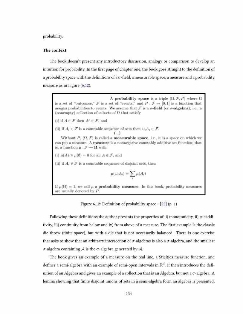
probability.

The context

The book doesn’t present any introductory discussion, analogy or comparison to develop an

intuition for probability. In the rst page of chapter one, the book goes straight to the denition of

a probability space with the denitions of a σ-eld, a measurable space, a measure and a probability

measure as in Figure (6.12).

Figure 6.12: Denition of probability space - [22] (p. 1)

Following these denitions the author presents the properties of: i) monotonicity, ii) subaddi-

tivity, iii) continuity from below and iv) from above of a measure. The rst example is the classic

die throw (nite space), but with a die that is not necessarily balanced. There is one exercise

that asks to show that an arbitrary intersection of σ-algebras is also a σ-algebra, and the smallest

σ-algebra containing A is the σ-algebra generated by A.

The book gives an example of a measure on the real line, a Stieltjes measure function, and

denes a semi-algebra with an example of semi-open intervals in Rd. It then introduces the de-

nition of an Algebra and gives an example of a collection that is an Algebra, but not a σ-algebra. A

lemma showing that nite disjoint unions of sets in a semi-algebra form an algebra is presented,

134

followed by an example of such an extension.

The author then denes a measure on an algebra and presents a theorem (with the proof in

the appendix) that helps to extend a measure on a semi-algebra to the σ-algebra it generates. The

rest of the section lies outside our interest for this thesis because it extends the denition of a

probability measure on R to Rn.

The exercises

Figure 6.13: Venn diagram - Exercises from [22]

Durrett’s book is the one with the smallest set of exercises. Out of six exercises from the

section, one makes the students work with the axiomatic denition of probability and the other

ve work exclusively with measure theory. Among those measure theory exercises, two concern

the denition of an algebra and three the generation of a σ-algebra.

6.3.10 Discussion

The book of Durrett is very direct and introduces no context for the denition of probability.

It states the denition of probability followed by some properties and one general example of a

discrete probability space (nite and innite). There is one line where he says: “In many cases when

Ω is a nite set, we have p(ω) = 1/|Ω|”, but this shy statement is not illustrated throughout the

text, except in that phrase. The less attentive, or unaware reader may not notice the importance

of that restriction to the cases when Ω is nite. Another characteristic of this book is that is

doesn’t require a previous course in measure theory. Concepts such as σ-algebra, semi-algebra

135

and measure are introduced along with the probability ideas. Most of the analyzed exercises focus

on measure theory and the ideas purely in probability seem to be of secondary importance.

6.4 Final remarks

While exercises in textbooks may be tools for students to practice a technique, if understand-

ing requires confronting and surmounting epistemological obstacles, exercises should help stu-

dents confront their beliefs and previous inadequate knowledge. They should help students testing

whether they have grasped the right idea of a specic denition, theorem, property or if they are

aware of subtle consequences of the mathematical content in focus. Exercises also help students

becoming aware of which ideas are the most important. In other words, exercises give clues to

students of what is the knowledge they are expected to learn. When students start learning a new

subject, it’s natural that they don’t have the mathematical maturity to distinguish and keep in

mind the most important ideas out of a myriad of information and less important facts by simply

reading the textbook.

The ve books that we’ve analyzed provide much emphasis on counting techniques, set op-

erations and measure theory facts, to the detriment of the innovations that modern probability

brought, such as the axiomatic denition and the ability to handle innite sample spaces. The

undergraduate level books reinforce the classical approach by showing the trivial and classical

examples of the coin toss and die throw and also by proposing a great number of exercises that as-

sociate proportional reasoning in a nite sample space with probability. The graduate level books

show less of a tendency to associate probability to proportional reasoning. On the other hand, they

concentrate a great deal of eort on set operations and measure theory exercises, leaving aside the

innovations brought by Kolmogorov.

We recognize the value in including well known examples, such as the coin toss or the die

throw. Not only will most students recall these scenarios from earlier courses, but this type of tan-

gible real-world event can oer a more palatable introduction to more abstract concepts. Further-

more, we are not denying or neglecting the importance that set operations, counting techniques

and measure theory deserve when it comes to probability. However, our analysis points out : i) the

limitation of examples and exercises to the very simple cases where the classical approach with the

ideas of nite probability spaces and proportional reasoning are reinforced in the undergraduate

136

level books and, ii) that working almost exclusively with measure and set theory ideas that require

little (or occasionally no) knowledge of probability may deviate the focus from the key concepts

to be learned in the graduate level books.

The book by Wackerly (and others)[68] has a more intuitive than formal approach. It discusses

how the relative frequency ts in with the axioms, however the treatment is concentrated in nite

sample space situations. Despite their mention of countable additivity in the third axiom, the

situations presented in the book largely reinforce probability as a proportional reasoning in a

nite sample space and no importance to the innovations brought by Kolmogorov is given. While

Wackerly (and others) reduces the importance of the axioms when they say that all real world

situations t in the relative frequency perspective, Ross[52] justies the axiomatization by saying

that the relative frequency may fail, so we need rst to dene a set of axioms and then verify

that the relative frequency, when the limit exists, ts those axioms. Ross also reinforces the idea of

probability as a proportional reasoning in a nite sample space via the exercises as well as through

a section with 15 examples of those cases. The section that discusses the continuity of probability

is left as an optional topic, doesn’t have any exercises and is not related to countable additivity.

Unlike the rst two books analyzed, the book of Grimmet and Sirzaker[27] is not meant to

be used in an introductory course. It advances with an example that shows the need for a σ-

algebra when considering innite spaces and mentions some topics related to a modern approach,

but doesn’t detail any of them. Most of the exercises also place an emphasis on proportional

reasoning, counting techniques, additivity and set operations, which drives the attention away

from the modern approach.

Shiryaev’s book [59] presents the distinction between the classical and the modern approach

more clearly, and explicitly, than the others. The text presents the denition of an algebra for nite

sample spaces and when it extends to innite spaces in chapter two, there is an example that shows

that the approach to probability needs to be changed. It also gives examples of a non-measurable

set and connects countable additivity with the continuity of probability. The drawback is the lack

of examples in the second chapter and the fact that the exercises that are provided concentrate

heavily on measure theory and set operations rather than on the modern denition of probability.

Like Shiryaev, Durrett’s book [22] doesn’t associate probability with a proportional reasoning. It

actually introduces many ideas from the modern approach. However, the book is goes directly into

the denitions and doesn’t present any discussion that would develop any intuition of probability

137

or any importance of certain concepts and ideas. As this books requires a more abstract and

sophisticated reasoning than the previous ones, it is not meant for a rst course in probability.

A nal remark on this book is that the focus on measure theory content may drive the attention

away from probability.

As presented in chapter four of this thesis and in Von Plato [67], the real world doesn’t possess

the symmetries of the classical theory, and the approach presented in the undergraduate analyzed

books can be harmful because rather than provoking the reader to confront and overcome the

epistemological obstacles of equiprobability and proportionality, they may actually be reinforcing

them. In the case of the graduate books we analyzed, the focus may deviate the attention from

these obstacles. Hence, the main critiques we present here are that when dening probability,

giving examples and proposing exercises, we should go beyond trivial examples and concern our-

selves with how much the example and exercises make students work with probability or other

mathematical contents. While simple examples set students in a familiar context to understand

probability, and measure and set theory are crucial to probability as we’ve shown in chapter 4, our

point is that simple examples and other mathematical contents should be present in the books,

but the focus should be changed, to illustrate some of the key aspects introduced by Kolmogorov’s

work driving the students from the classical towards the modern thinking in probability.

138

Chapter 7

Final Remarks

The objective of this thesis was to answer two main questions, the rst concerning the history

and foundation of probability and its association with measure theory. If probability has been

present in mathematics for many centuries, why did the advent of measure theory immediately

reveal a very strong relationship between these two branches of mathematics, establishing prob-

ability as a measure between 0 and 1? More specically, why did probability need measure theory

as its basis to be considered an autonomous branch of mathematics? By understanding this evo-

lution from classic to modern probability and the importance of Kolmogorov’s axiomatization, a

second main research question that attaches a didactical value to this thesis emerged: Considering

the classical and the modern approaches to probability, which one of them are primarily advanced

by undergraduate and graduate textbooks?

7.1 Remarks on the history and foundation of probability

Bernoulli and de Moivre published the rst works that dened probability, starting what we

have called in this thesis the classical approach. We consider them the founders of probability

as science due to the great level of generality of their denitions of probability and expectation.

Despite the advances made by Cardano, Pascal and Huygens among others, their works were

limited to resolution of specic problems, while Bernoulli and de Moivre dened probability as a

general concept: the ratio of favourable over possible outcomes. Bernoulli also stated and proved,

with full rigour, the rst version of the weak law of large numbers.

Classical probability was considered a branch of applied mathematics. With its development,

139

probability provided formulas for error terms, statistical physics and solutions to problems in

games of chance, however not much attention was given to the mathematical basis of that prob-

abilistic context. The concepts and methods were specic to applications, and their contributions

to larger questions of science and philosophy were limited. The classical denition remained es-

sentially the same throughout the 18th and 19th centuries. Yet, as science evolved through time,

the lack of precision of some associated concepts such as random variables and events, and some

contradictory results began to evidence the limitations of that denition of probability.

The modern and axiomatic denition of probability in its complete and abstract form could

not be developed until the advent of measure theory. The denition of measurable sets broadened

the type of sets for which we can evaluate the probability. The Carathéodory’s extension theo-

rem or the equivalent probability version by Kolmogorov relied heavily on countable additivity.

Lebesgue’s integral allowed the proof of many convergence theorems involving limits of integrals.

Fréchet took Lebesgue’s integral beyond Euclidean spaces and the Radon-Nikodyn theorem devel-

oped the integral in full abstraction, providing a way to evaluate the probability of a set conditional

to a σ-algebra, which made it possible to see conditional probability as a random variable and also

to evaluate probability conditional to sets of measure zero.

The rst probability works that used measure theory came form Anders Wiman in 1900 and

Weyl in 1909. This relationship was consolidated by Hausor in 1914. Despite the association

between the disciplines, the modern denition of probability was still to be created. Besides Haus-

dor’s work in set theory, Borel’s use of countable additivity, his strong law of large numbers and

the dierent demonstrations from Hardy and Littlewood, Hausdor, Khinchin and Kolmogorov,

made important contributions in that direction.

Rather than proceeding with a purely chronological exposition, we tried, as much as possible,

to explore the main ideas, even the blind alleyways, that led to the axiomatization of probabil-

ity based on measure theory. These imprecise and contradictory developments are important for

scientic evolution. The history of mathematics cannot be limited to the results in the standard

textbooks, and probability is not an exception. The early and unsuccessful attempts at an axiomati-

zation from Laemmel, Broggi, Hilbert, Lomnicki, Ulam, von Mises, Slutsky and Steinhaus provided

important insights to the advance of probability.

Besides the failed attempts at an axiomatization, successful developments were also important.

140

Daniell’s integral of a linear operator with examples in innite-dimensional spaces, Wiener’s for-

malization of the notion of Brownian motion and Ville’s concept of martingales are examples in

that direction. Other works from Kolmogorov also made signicant progress towards modern

probability before the axiomatization. In particular, we note his articles of 1925, on convergence

of random events, and 1928, on convergence of the sum of random variables. His article of 1929

improved the association of measure and probability using a countable additive function and his

work of 1931 developed continuous time Markov chains using countable additivity.

If one takes into consideration all of those contributions, it is not hard to conclude that Kol-

mogorov’s Foundations of the Theory of Probability is a work of synthesis. Kolmogorov was the

mathematician who was able to identify the valuable ideas of his predecessors among the myriad

of statements to t existing knowledge into a new approach. To do justice to the scope of his

book, beyond the synthesis and the axiomatic denition, there are also a number of innovations

that must be taken in consideration: i) probability distributions in innite-dimensional spaces,

ii) dierentiation and integration of mathematical expectations with respect to a parameter and

iii) a general treatment of conditional probabilities and expectations based on Radon-Nikodyn’s

theorem that allowed us to evaluate probabilities conditioned to measure zero sets.

As Kolmogorov mentions, his developments arose of necessity from some concrete physical

problems. Quantum mechanics viewed the elementary processes in nature as non-deterministic

and modern probability played (and still plays) an essential role in describing those processes.

We’ve exposed how Kolmogorov’s book constructed the axiomatization in two chapters of

his book. In the rst one, he presented ve axioms considering a nite sample space. The main

contribution there is the set of axioms that formalized and generalized the classical denition in

nite spaces. The second chapter added another innovation to the denition, because it reaches its

full generality when Kolmogorov introduced axiom VI (continuity 1) and formalized probability

to innite spaces. We’ve also described the concepts of probability functions, random variables,

conditional probability and conditional mathematical expectation in the modern approach. After

the denition of those terms, we used modern probability to resolve the great circle paradox as an

illustration of how this approach established a rigorous basis free of ambiguities. The paradox in

the great circle arises from a mistaken application of elementary conditional probability, coming1or equivalently, countable additivity

141

from a naïve application of symmetry2 that leads to an application of a 1-dimensional Lebesgue

measure in a situation where it should be 2-dimensional.

7.2 Remarks on the didactical implications

The understanding of this evolution from the classic to the modern approach to probability

made us think about students’ understanding of the denition of probability and the approach

that books advance through the exposition and the exercises.

After a discussion into the concepts of epistemologial obstacles in mathematics and in proba-

bility, we’ve identied a great scarcity of studies involving probability teaching and learning at a

post-secondary level. Many studies have been done concerning elementary or high school students

and a great measure of those are dedicated to conditional probability, randomness, and represen-

tativeness of samples. However, there is a lot of research to be done in students’ understanding of

the denition of probability at the post-secondary level.

Given the shortage of research in post-secondary probability education, we’ve done a pilot test

with a few graduate students from mathematics and statistics programs to obtain some insights

into their conceptualization of probability. In order to accomplish this, we exposed them to a situ-

ation where they needed to deal with an innite space, where the classical approach is ineective.

We’ve identied the persistence of the equiprobability and proportionality obstacles in those stu-

dents. In probability, these epistemological obstacles come from the habit of using proportional

reasoning in nite spaces with equally likely events, which reinforces a classical approach to prob-

ability.

Once those obstacles were identied, we decided to investigate some undergraduate and grad-

uate textbooks used in the four universities in Montreal with the goal of identifying how those

books introduce the denition of probability and help develop, though the exercises, a modern or

a classic view of the subject.

The main conclusion that we were able to draw from this analysis, was that too much emphasis

is given to counting techniques, set operations and, for the graduate level, measure theory facts,

and the innovations that modern probability brought play a secondary role. The undergraduate

level books reinforce the classical approach by showing the trivial and classic examples of the coin2or the principle of indierence

142

toss and die throw as well as by proposing tasks that, for the most part, stimulate an association of

probability with proportional reasoning in a nite sample space. The graduate level books don’t

show the same tendency of attaching a linear reasoning to probability as do the undergraduate

ones. They do, however, encourage students to concentrate their eorts on exercises whose con-

tent is almost exclusively drawn from set and/or measure theory, many of them not demanding

any knowledge of probability at all.

Simple and trivial examples such as the die throw and coin toss don’t do harm in and of them-

selves. In fact, it can be benecial to consider a classic example to begin with, because it puts the

student in a familiar setting that can enhance their condence for learning probability. Addition-

ally, we don’t deny the importance of set operations, counting techniques and measure theory to

probability and we don’t advocate for the removal of those exercises from the books. Our critiques

here addresses to the (almost) exclusiveness of exercises that stimulate a proportional reasoning

and an equiprobability view of sets, in a classical probability context, in the case of the undergrad-

uate books, and the focus on almost exclusively measure and set theory tasks with little probability

knowledge requested, in the case of the graduate books.

The approach presented in the books analyzed can be harmful, because instead of overcoming

the epistemological obstacles of proportionality and equiprobability, they may be actually reinforc-

ing them, in the case of undergraduate level, or deviating the attention from them in the case of

the graduate level. When choosing examples and exercises, we suggest that the instructor should

consider the weight given to classical probability, modern probability or other mathematical con-

tents. Our main point here is that simple examples and other mathematical concepts should be

present in the recommended texts (or in the lectures), but the focus should be changed, to illustrate

some aspects introduced by Kolmogorov’s work that drive the students from the classical towards

the modern thinking in probability.

7.3 Originality, limitations and future research

One of the elements of originality of this thesis is the use of original sources to evidence a few

mathematical ideas, or to present in detail some proofs, from each author’s contribution to the

foundations of modern probability. The didactical contribution is also original, because there is

a scarcity of research in the pedagogy pertaining to the teaching and learning of probability at a

143

post-secondary level.

This thesis is limited to some ideas of the evolution of probability. We did not attempt to

outline the entire history of probability theory; detailing every development and every proof is

well beyond the scope of this work. Rather, we focused on some main ideas and detailed the

proofs of some important results.

Some important original sources were not accessible in English or French. For example, Carathéodory’s

work on axioms for measure theory or his extension theorem and Hausdors book in set theory,

with important insights in probability, were only accessible in German3.

Our pilot test is concentrated with a very small sample extracted from a restricted population.

The results achieved in this test were mainly used as preliminary ones to bring insight into further

investigation. Instead of the students’ conceptualization of probability, the focus of our research

was the analysis of the theory and exercises presented in ve books typically chosen in the four

universities in Montreal for undergraduate and graduate courses in probability.

We surmise that if students at the graduate level in mathematics don’t display a modern think-

ing of probability, undergraduate students, or students from dierent disciplines will not display

this modern thinking either.

In future research, this study could be extended to a larger sample of students and from dif-

ferent areas that are highly connected to probability, such as engineering or computer science. In

the case of other disciplines, one may question what is at stake, if anything, if professionals don’t

develop a modern approach to probability.

Further questions could concern dierence between students who have a background in mea-

sure theory and those who have none. If dierences exists, which elements of measure theory,

and what didactic approach, would help students developing a modern approach to probability?

In particular, what type of tasks (exercises) would help students reecting on a modern approach

to probability and understanding the importance and shortcomings of the classical approach?

3There is an English translation, but it is abbreviated and the chapter that discusses probability has been omitted.

144

Bibliography

[1] ANAGNOSTOPOULOS, C. Bertrand paradoxes and kolmogorov’s foundations of the theory

of probability. Master’s thesis, University of Athens, 2006.

[2] ASH, B. R., and DOLÉANS-DADE, C. Probability and Measure Theory. Harcout Academic

Press, New York, 2000.

[3] BACHELARD, G. La formation de l’esprit scientique : contribution à une psychanalyse de la

connaissance objective, 5 ed. J. Vrin, Paris, 1967.

[4] BARONE, J., and NOVIKOFF, A. A history of the axiomatic formulation of probability from

borel to kolmogorov: Part i. A. Arch. Hist. Exact Sci. 87, 18 (1978), 123–190.

[5] BARTLE, R. Elements of integration and Lebesgue measure. John Wiley & Sons, New York.,

1995.

[6] BAYES, T. An essay towards solving a problem in the doctrine of chances. by the late rev. mr.

bayes, f. r. s. communicated by mr. price, in a letter to john canton, a. m. f. r. s. Philosophical

Transactions 53 (1763), 370–418.

[7] BERNOULLI, J. The art of conjecturing, together with Letter to a friend on sets in court tennis /

by Jacob Bernoulli; translated with an introduction and notes by Edith Dudley Sylla. The Johns

Hopkins University Press, Baltimore, USA., 2006.

[8] BERTRAND, J. Calcul des probabilités. Chelsea Publishing Company, New York, USA., 1907.

[9] BINGHAM, N. H. Studies in the history of probability and statistics xlvi. measure into prob-

ability: From lebesgue to kolmogorov. Biometrika 87, 1 (2000), 145–156.

[10] BOREL, E. Sur quelques points de la théorie des fonctions, vol. 12. Gauthier-Villars, 1894.

145

[11] BOREL, E. Leçons sur la théory des fonctions. Gauthier-Villars et Fils, Paris., 1898.

[12] BOREL, E. Remarques sur certaines questions de probabilité. Bulletin de la S. M. F. 33 (1905),

123–128.

[13] BOREL, E. Les probabilités dénombrables et leurs applications arithmétiques. Rendiconti del

Circolo Matematico di Palermo 27 (1909), 247–271.

[14] BOROVCNIK, M., and KAPADIA, R. A historical and philosophical perspective on probabil-

ity. In Probabilistic Thinking. Springer, 2014, pp. 7–34.

[15] BROUSSEAU, G. P. Les obstacles épistémologiques et les problèmes en mathématiques. In La

problématique et l’enseignement de la mathématique. Comptes rendus de la XXVIIIe rencontre

organisée par la Commission Internationale pour l’Etude et l’Amélioration de l’Enseignement des

Mathématiques, W. V. et Jacqueline Vanhamme, Ed. Louvain-la-neuve, 1976, pp. 101–117.

[16] BROUSSEAU, G. P. Les obstacles épistémologiques, problèmes et ingénierie didactique. In

La théorie des situations didactiques, G. Brousseau, Ed., Recherches en Didactiques des Math-

ématiques. La pensée sauvage, 1998, pp. 115–160.

[17] BYERS, W. How mathematicians think: Using ambiguity, contradiction, and paradox to create

mathematics. Princeton University Press, 2010.

[18] COURNOT, A. A. Exposition de la théorie des chances et des probabilités. L. Hachette, 1843.

[19] DAVIS, P., H. R., and MARCHISOTTO, E. A. The mathematical experience. Springer Science

& Business Media, 2011.

[20] De BOCK, D., VAN DOOREN, W., JANSSENS, D., and VERSCHAFFEL, L. Improper use of

linear reasoning: An in-depth study of the nature and the irresistibility of secondary school

students’ errors. Educational studies in mathematics 50, 3 (2002), 311–334.

[21] DEMOIVRE, A. The Doctrine of Chances: or, a method of calculating the probabilityes of events

in play. Chelsea Publishing Company, New York., 1967.

[22] DURRETT, R. Probability: theory and examples. Cambridge university press, 2010.

[23] FREUDENTHAL, H. Mathematics as an educational task. D. Reidel Publishing Company,

Dordrecht, NL, 1973.

146

[24] FRÉCHET, M. Sur l’intégrale d’une fonctionelle étendue à un ensemble abstrait. Bulletin de

la S. M. F. 43 (1915), 248–265.

[25] GAUVRIT, N., and MORSANYI, K. The equiprobability bias from a mathematical and psy-

chological perspective. Advances in Cognitive Psychology 10, 4 (2014), 119 – 130.

[26] GILLISPIE, C. C., HOLMES, F. L., and KOERTGE, N., Eds. Complete Dictionary of Scientic

Biography. Charles Scribner’s Sons, Detroit, 2008.

[27] GRIMMETT, G., and STIRZAKER, D. Probability and random processes. Oxford university

press, 2001.

[28] GRINSTEAD, C. M., and SNELL, J. L. Introduction to probability. American Mathematical

Soc., 2012.

[29] GYENIS, Z., HOFER-SZABO, G., and RÉDEI,M. Conditioning using conditional expectations:

the borel-kolmogorov paradox. Synthese 194, 7 (2017), 2595–2630.

[30] HALD, A. A History of Probability and Statistics and Their Applications before 1750. John

Wiley & Sons, Inc, New Jersey, 2003.

[31] HARDY, G. H., and LITTLEWOOD, J. E. Some problems of diophantine approximation: Part

i. the fractional part of nkθ. Acta Math. 37 (1914), 155–191.

[32] HARDY, N. Students’ Models of the knowledge to be learned about limits in college level calculus

courses. The inuence of routine tasks and the role played by institutional norms. PhD thesis,

Concordia University, 2006.

[33] HAWKINS, T. Lebesgue’s Theory of Integration: its origins and development. Chelsea Publish-

ing Company, New York., 1975.

[34] HOCHKIRCHEN, T. Theory of measure and integration from riemann to lebesgue. In A

History of Analysis, H. N. JAHNKE, Ed., vol. 24. American Mathematical Society, Providence,

USA, 2003, ch. 9, pp. 261–290.

[35] KOLMOGOROV, A. General measure theory and calculus of probabilities (1929). In Se-

lected Works of AN Kolmogorov: Vol. 2, Probability Theory and Mathematical Statistics, A. N.

SHIRYAEV, Ed. Springer, Berlin, 1992, pp. 48–58.

147

[36] KOLMOGOROV, A. On analytical methods in probability theory (1931). In Selected Works of

AN Kolmogorov: Vol. 2, Probability Theory and Mathematical Statistics, A. N. SHIRYAEV, Ed.

Springer, Berlin, 1992, pp. 62–108.

[37] KOLMOGOROV, A. On sums of independent random variables (1928). In Selected Works of

AN Kolmogorov: Vol. 2, Probability Theory and Mathematical Statistics, A. N. SHIRYAEV, Ed.

Springer, Berlin, 1992, pp. 15–31.

[38] KOLMOGOROV, A., and Khinchin, A. Y. On convergence of series whose terms are de-

termined by random events (1925). In Selected Works of AN Kolmogorov: Vol. 2, Probability

Theory and Mathematical Statistics, A. N. SHIRYAEV, Ed. Springer, Berlin, 1992, pp. 1–10.

[39] KOLMOGOROV, A. N. Foundations of the Theory of Probability. Chelsea Publishing Company,

New York., 1956.

[40] LAMPRIANOU, I., and AFANTITI LAMPRIANOU, T. The nature of pupils’ probabilistic

thinking in primary schools in cyprus. In PME CONFERENCE (2002), vol. 3, pp. 173–180.

[41] LAPLACE, P. S. Théorie analytique des probabilités. Courcier, Paris, 1814.

[42] LEAO Jr, D., FRAGOSO, M., and RUFFINO, P. Regular conditional probability, disintegration

of probability and radon spaces. Proyecciones (Antofagasta) 23, 1 (2004), 15–29.

[43] LEBESGUE, H. Intégrale, longueur, aire. Annali di Matematica Pura ed Applicata (1898-1922)

7, 1 (1902), 231–359.

[44] LEBESGUE, H. Leçons sur l’intégration et la recherche des fonctions primitives. Gauthier-Villars

et Fils, Paris., 1904.

[45] LECOUTRE, M.-P. Cognitive models and problem spaces in "purely random" situations. Ed-

ucational Studies in Mathematics 23, 6 (1992), 557–568.

[46] MAISTROV, L. E. Probability Theori: A historical sketch. Academic Press, New York, 1974.

[47] MISZANIEC, J. Designing eective lessons on probability. a pilot study focused on the illusion

of linearity. Master’s thesis, Concordia University, 2016.

148

[48] MORSANYI, K., PRIMI, C., CHIESI, F., and HANDLEY, S. The eects and side-eects of

statistics education: Psychology students’ (mis-)conceptions of probability. Contemporary

Educational Psychology 34, 3 (2009), 210 – 220.

[49] PIAGET, J., and INHELDER, B. The Origin ofthe Idea of Chance in Children. Norton, New

York, 1975.

[50] PIER, J. P. Intégration et mesure 1900-1950. In Development of Mathematics 1900-1950, J. P.

PIER, Ed. Birkhäuser, Berlin, 1994, ch. 11, pp. 517–564.

[51] POINCARÉ, H. Calcul des Probabilités. Deuxième édition revue et augmantée par l’auteur.

Gauthier-Villars, Imprimeur-Libraire, Paris., 1912.

[52] ROSS, S. A First Course in Probability 8th Edition. Pearson, 2009.

[53] ROYDEN, H. L., and FITZPATRICK, P. M. Real Analysis. Pearson Education, New York., 2010.

[54] RUBEL, L. H. Middle school and high school students’ probabilistic reasoning on coin tasks.

Journal for Research in Mathematics Education (2007), 531–556.

[55] SCHOENFELD, A. H. Learning to think mathematically: Problem solving, metacognition,

and sense making in mathematics. In Handbook of research on mathematics teaching and

learning, D. GROUWS, Ed. Macmillan Publishing Co, Inc, New York, 1992, pp. 334–370.

[56] SHAFER, G., and VOVK, V. The Sources of Kolmogorov’s Grundbegrie. Statistical Science

21, 1 (2006), 70–98.

[57] SHAUGHNESSY, J. Research in probability and statistics: Reections and directions. InHand-

book of research on mathematics teaching and learning, D. GROUWS, Ed. Macmillan Publish-

ing Co, Inc, New York, 1992, pp. 465–494.

[58] SHAUGHNESSY, J. M. Misconceptions of probability: An experiment with a small-group,

activity-based, model building approach to introductory probability at the college level. Ed-

ucational Studies in Mathematics 8, 3 (1977), 295–316.

[59] SHIRYAEV, A. N. Probability-1. Third Edition. Translated by R.P. Boas: and D.M. Chibisov.

Springer, New York, 2016.

149

[60] SIERPINSKA, A. Humanities students and epistemological obstacles related to limits. Edu-

cational studies in Mathematics 18, 4 (1987), 371–397.

[61] SIERPINSKA, A. Some remarks on understanding in mathematics. For the learning of math-

ematics 10, 3 (1990), 24–41.

[62] SIERPINSKA, A. Understanding in Mathematics. Studies in Mathematics Education Series.

Falmer Press, London, 1990.

[63] STEINHAUS, H. Les probabilités dénombrables et leur rapport à la théorie de la mesure.

Fundamenta Mathematicae 4, 1 (1923), 286–310.

[64] van DALEN, D., and MONNA, A. F. Sets and integration: an outline of the development.

Wolters-Noordho Publishing, Groningen, The Netherlands., 1972.

[65] Van DOOREN, W., De BOCK, D., DEPAEPE, F., JANSSENS, D., and VERSCHAFFEL, L. The

illusion of linearity: Expanding the evidence towards probabilistic reasoning. Educational

studies in mathematics 53, 2 (2003), 113–138.

[66] VILLE, J. Étude critique de la notion de collectif. Gauthier-Villars Paris, 1939.

[67] VON PLATO, J. Creating Probability: its mathematics, physics and philosophy in historical

perspective. Cambridge University Press, New York, 1994.

[68] WACKERLY, D., MENDENHALL, W., and SCHEAFFER, R. L. Mathematical statistics with

applications. Cengage Learning, 2014.

[69] WATSON, J. M., and MORITZ, J. B. Fairness of dice: A longitudinal study of students’ beliefs

and strategies for making judgments. Journal for research in mathematics education (2003),

270–304.

150