The sentiment bias in the market for tennis betting sentiment bias in the market for tennis betting...
49
The sentiment bias in the market for tennis betting Saskia van Rheenen 347986 Behavioural Economics April 2017 Supervisor dr. T.L.P.R. Peeters Second reader dr. G.D. Granic
Transcript of The sentiment bias in the market for tennis betting sentiment bias in the market for tennis betting...

The sentiment bias in the market for tennis betting
Saskia van Rheenen
347986
Behavioural Economics
April 2017
Supervisor
dr. T.L.P.R. Peeters
Second reader
dr. G.D. Granic

2
TABLE OF CONTENTS
List of Tables 3 1. Introduction 4 2. Theoretical framework 7
2.1 The sports betting market 2.2 Reasons for betting 2.3 Types of bettors 2.4 Market efficiency in the betting market
2.4.1 The Efficient Market Hypothesis 2.4.2 The sentiment bias 2.4.3 The favorite-longshot bias
2.5 The role of bookmakers 2.5.1 Balance the books 2.5.2 Set the market-clearing price 2.5.3 Active odds setting
7 9
11 12 12 12 14 14 14 15 16
3. Literature review 17 4. Hypotheses 5. Data
5.1 Betting data 5.2 Google Trends data 5.3 The final dataset
6. Methodology 6.1 The probit model 6.2 Model estimation 6.3 Goodness-of-fit
21 23 23 24 26 27 27 29 30
7. Results 7.1 Summary statistics 7.2 The full sample
7.2.1 Regression results 7.2.2 Unit Bet & Unit Win
7.3 Sentiment bias in tournament finals 7.4 Sentiment bias in matches of the Big Four 7.5 Exploiting the sentiment bias
7.5.1 The full sample 7.5.2 The tournament finals 7.5.3 The Big Four
30 30 32 32 33 33 35 36 36 37 37
8 Conclusion 37 9 Limitations and future research 40 References 41 Appendices 45
A. An overview of the ATP World Tour B. Probit model using random sampling C. The Average Partial Effects (APE) D. Analysis of the favorite-longshot bias
45 46 47 48

3
LIST OF TABLES
1. Decimal odds for the 2016 Australian Open final
2. An example of a set of odds for which a bookmaker makes a loss
3. An overview of the most important studies regarding the sentiment bias
4. Number of missing observations for each bookmaker 5. Correlation between the different bookmakers 6. Summary statistics
7. Clustered probit regression results
8. Profits for Unit Bet and Unit Win strategies
9. Clustered probit regression results Final and Non-final samples
10. Clustered probit regression results Big-Four and Non-Big Four samples
B1. Probit regression results random sampling
C1. The Average Partial Effect (APE)
D1. Z-test statistics
7
9
20
26
26
31
32
33
35
35
46
47
49

4
1. Introduction
In 2004, Gerry McIlroy placed a $200 bet on that his son would win the British Open before
turning 25. Rory McIlroy managed to do this and his dad won $171,000 (Johnson, 2014).
This is an example of people placing bets for reasons other than the objective outcome
probability of an event. This market inefficiency is called the sentiment bias, defined by
Avery and Chevalier (1999) as "any non-maximizing trading pattern among noise traders that
can be attributed to a particular exogenous motivation" (p. 493). The main objective of this
research is to determine to which degree the sentiment bias is present in the market for tennis
betting. The findings challenge market efficiency because bookmaker odds do not reflect the
true outcome probability. They strategically set the odds to rationally exploit sentimental
bettor preferences. Bookmakers underestimate the winning probability for the high-sentiment
players in tournament finals and in matches with any of the Big Four1. As a result of this
reversed sentiment bias, bookmakers offer a relatively high price for bets on popular players.
The mispricing cannot be profitably exploited, but improves returns from placing random
bets.
This study uses odds for men's single Grand Slam2 matches in seasons 2000-2016. The
betting data is merged with a measure that reflects the level of sentiment that bettors have for
a player, namely the number of searches on Google. It is assumed that Google Trends data is
a proxy for all sources of sentiment that create popularity.3 Grand Slam tournaments are of
most interest for four reasons. First of all, Grand Slams are played in a best-of-five sets format
instead of the usual best-of-three sets. This implies longer matches that are less likely to be
decided by a random event other than the players' performance, which minimizes noise. For
this reason, women's matches (always played in best-of-three format) are left out. Second,
Grand Slam tournaments pay out higher prize money and emit a high level of prestige. As a
result, players will put in more effort to win a match, whereas they have the tendency to tank
a match in low-tiered tournaments every now and then. For the same reasons there is a lower
chance of match fixing in Grand Slam tournaments, which reduces the noise. Third, Grand
Slam tournaments attract most attention from fans. This implies that they are responsible for
the highest share of betting volume in tennis. This emphasizes the economic value of this
research. Additionally, a higher number of market participants implies higher market 1 The Big Four consists of Roger Federer, Rafael Nadal, Novak Djokovic and Andy Murray. 2The four Grand Slams are the Australian Open, the French Open (Roland Garros), Wimbledon and the US Open. 3 Bad behavior and unsportsmanship might lead to a higher amount of Google searches, which will as a result be included in the popularity measure. This makes sense, as negative sentiment can make a player popular as well. Nick Kyrgios is an example of a tennis player misbehaving on and off the court. Despite (or because of) his bad reputation, he is box office for tournament directors and fans because his matches always have a high entertainment value. (Steinberger, 2016).

5
efficiency, so this minimizes the noise. The fourth interesting feature of studying Grand Slam
tournaments is the large draw (128 players, of which 16 qualifiers and 8 wildcards), which
contains players from a wide range of rankings. This allows studying the difference in
sentiment bias between matches of super star players (the Big Four) and less known players.
The tennis betting market is very suitable for examining the sentiment bias. First, it is an
international sport with a strong emotional attachment across borders. Players such as Roger
Federer and Rafael Nadal have active fan bases worldwide. Second, the way tennis
tournaments are structured allows the world number one to play someone who barely
qualified for the tournament. As explained by Forrest and McHale (2007), therefore, "this
market allows the analysis of wagering opportunities across almost the complete odds range
from zero to one probability-odds" (p. 754). Third, a tennis match has no possibility to end in
a draw. This is suitable for measuring sentiment bias because individuals do not feel
sentiment for a draw. Most importantly, the unambiguous outcome of a tennis match helps to
measure the underlying value of a bet, which is either a payout or a loss. Finally, a men's
single tennis match consists of only two players. This means that bettors have to process less
complex information compared to, for example, an entire soccer team. This can also be
framed as a measurement advantage. Do people place bets on Real Madrid because it is a
popular club or rather because they like Christiano Ronaldo? This ambiguity is not present in
the market for tennis betting, which leads to a clearer measurement.
Levitt (2004) mentions three parallels between trading in financial markets and betting
markets. First of all, individuals in both markets are heterogeneous, profit-maximizing
investors with different information levels, dealing with risk that diminishes over time until
the trading period is over. Secondly, both market are zero-sum games, with one trader on each
side of the deal. Finally, large amounts of money are at stake in both markets.
Important differences between the two markets exist as well, which make it hard to translate
concluding remarks from this study into theories for financial markets. Sports betting markets
are simple financial markets and therefore suitable to study the information content of market
prices (Sauer, 2005). The main advantage of the sports betting market is that "it is
characterized by a well-defined termination point at which each asset (or bet) possesses a
definitive value" (Williams, 1999, p. 1). As mentioned previously, the impossibility of a draw
leads to a binary and clear termination value. This is contrary to financial markets, where the
value of an asset depends on both the discounting of future cash flows and the uncertain price
market players are willing to pay for the asset (Thaler & Ziemba, 1988). A second
dissimilarity between the two is that the existence of well-informed traders, and in turn

6
market efficiency, is more likely in betting markets. The complexity of valuing assets in
financial markets and the increased level of inside information make it difficult for
individuals to become well-informed traders and collect superior information that noise
traders do not have.
The first research question of this study is whether bettor sentiment affects the odd-setting
strategy of bookmakers in the market for tennis betting. If so, there is market inefficiency.
Second, I ask whether there is a difference in how bookmakers respond to the sentiment bias
in earlier rounds compared to tournament finals. Third, this research analyzes the effect of the
presence of the Big Four on the bookmaker pricing strategy. I ask whether the response to
bettor sentiment is higher for matches of these players. If, in any of the samples, there is
evidence for sentiment bias, the final research question is whether well-informed traders can
profitably exploit the bias. Depending on the direction of the sentiment, this is equivalent to
the monetary value of engaging in a betting strategy against or in favor of the high-sentiment
players.
This research contributes to the existing literature in two ways. First of all, previous studies
have primarily documented the favorite-long shot bias: bettors tend to over bet the underdog
and under bet the favorite. The robustness of this inefficiency has been tested extensively
(Abinzano, Muga & Santamaria, 2016; Cain, Law & Peel, 2000; Gandar et al., 2002;
Williams & Paton, 1997; Woodland & Woodland, 1994), whereas research on the sentiment
bias is in a relatively early phase. Secondly, within the academic research on behavioral
biases, this is, to the best of my knowledge, only the second study to use data from the tennis
betting market. Forrest and McHale (2007) were the first to find market inefficiency in the
tennis betting market, in terms of the favorite-longshot bias. Previous studies have
documented the sentiment bias in the National Basketball Association [NBA], the National
Football League [NFL], the Premier League and the Primera División. The results were
ambiguous, which emphasizes the importance of additional research on this topic.
The next chapter provides the theoretical foundation of this research. This section is followed
by a literature review of existing research on the sentiment bias. Chapter 4 introduces the
hypotheses that will be tested in this study. Chapter 5 describes the data used to test the
hypotheses. Chapter 6 contains an explanation on the methodology. This is followed by
Chapter 7, which presents the results of the analyses. Chapter 8 concludes and discusses the
results. Finally, Chapter 9 discusses the limitations of this research and provides opportunities
for future studies.
7
2. Theoretical framework
2.1 The sports betting market
The global sports betting industry is expected to reach a gross revenue (stakes minus prizes)
of $70 billion in 2016 (ESSA Sports Betting Integrity, 2014). The exact worth is expected to
be much higher, however difficult to estimate because of the inconsistency of sports betting
regulation across the world. According to Adam Silver, NBA commissioner, the annual value
of illegal sports betting in the US is $400 billion (Weissman, 2014), which is only two-third
of the value of the illegal sports gambling market in China (Porteous, 2016). In Europe,
Internet betting is the biggest player, with bettors having the choice from several bookmakers.
Traditionally, the bookmaker acts as a trader announcing the prices against which bettors can
place their bets. In recent years, after the bookmaker has determined its odds, bets can also be
traded among bettors on online betting exchanges (Franck, Verbeek & Nüesch, 2010).
Bookmakers operate both in a service and information market (Kuypers, 2000). They offer
bettors a service by giving them the opportunity to place a bet. On the other hand it is an
information market because supply and demand lead to an equilibrium price, just like in any
other financial market. Bookmakers use two formats to express the odds on which bets can be
placed: point spreads and decimal odds.
Schnytzer and Weinberg (2007) define point spreads as "odds that a team will win by more
than a certain number of points, known as the line" (p. 6). In tennis, one can bet on the game
line and the set line. Matches in Grand Slam tournaments, on which this study is based, are
played in a best-of-five sets format. For these matches, the set line can be as high as 2.5. In
that case a player needs to win in straight sets for you to win the bet.
This study uses decimal odds, where "the bookmaker offers to pay a ratio of the amount
wagered if a certain team wins" (Schnytzer & Weinberg, 2007, p. 6). In tennis, this means that
there are two possible outcomes 𝑒 ∈ {𝑖, 𝑗}: either player i or j wins the match. These payout
ratios can have a very wide range, depending on the quality of the players in that match. As an
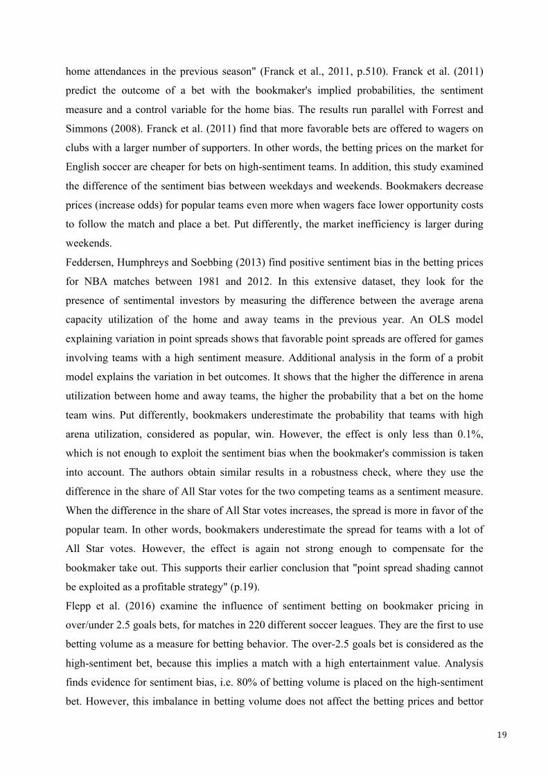
example, Table 1 presents the odds for the final of the 2016 Australian Open (Bet365, 2016).
Table 1. Decimal odds for the 2016 Australian Open final
Player Odds Player Odds Novak Djokovic 1.20 Andy Murray 5.15
Table 1 shows that a $1 bet on Novak Djokovic (Andy Murray) pays out $1.20 ($5.15) if he
wins the match. Obviously, the player with the lower odds is the favorite to win the match.

8
Dividing 1 by the decimal odds results in the corresponding 'probabilities' of that player
winning the match (Franck et al., 2010). In this case, the 'probabilities' of Novak Djokovic
and Andy Murray winning the match are 0.8333 and 0.1942, respectively. The sum of these
'probabilities' is larger than 1, which is because of the bookmaker's commission (Forrest &
Simmons, 2008). Therefore, they cannot be considered as the real winning probabilities until
they have been adjusted for the overround.
The betting market can be split into two frameworks: pari-mutuel (moving odds) betting and
fixed odds betting. Pari-mutuel betting is mainly used in horse racing, where fixed odds
betting is applied in both individual (tennis and boxing) and team sports (basketball,
American football and soccer). In a pari-mutuel betting environment, all bets on the
participating horses are put together in a pool. Next, the bookmaker's commission is taken
from the total amount wagered on the race. This is the profit for bookmakers and it is a fixed
percentage. In other words, pari-mutuel betting is a low-risk strategy for bookmakers, as their
income only depends on the amount of money that is bet on the race, but not on the outcome
of the race (Australia Sports Betting, 2016).
The fixed odds betting market is most relevant for this research, as this framework is used in
the tennis betting market. In contrast to the pari-mutuel structure, the odds that one receives
are fixed before the start of the match. However, the odds received may differ between
different bettors, depending on when they placed their bet. As in the pari-mutuel framework,
the odds change over time due to the quantity of additional bets placed. In the fixed odds
structure, however, you receive the odds stated at the moment you place the bet. As an
example, suppose that you place a bet on Roger Federer winning his first round at Wimbledon
2016, receiving the odds stated at the moment of placing your bet. Someone else places a bet
four hours later. In the meantime, additional bets have been placed on Roger Federer and
Guido Pella (his opponent) and the bookmakers have adjusted the odds. Therefore, you bet on
different odds than your fellow bettor, but the odds are fixed for both of you.
The main difference between the fixed odds and the pari-mutuel framework is the degree of
risk for bookmakers. The profit margin for bookmakers is uncertain in the fixed odds betting
market. The level of profit is different for every outcome of the match. This is why fixed odds
bookmakers, as a compensation for this risk, require a higher margin than pari-mutuel
bookmakers (Makropoulou & Markellos, 2011). It explains why bookmakers have a reason to
be more strategic in setting fixed odds than moving-odds. As a result, moving odds will be a
cleaner representation of bettor preferences. Bookmakers divert the fixed odds away from the
9
true winning probabilities to shield themselves from losses. Therefore, fixed odds betting is
the best market to measure violations of market efficiency, e.g. the sentiment bias.
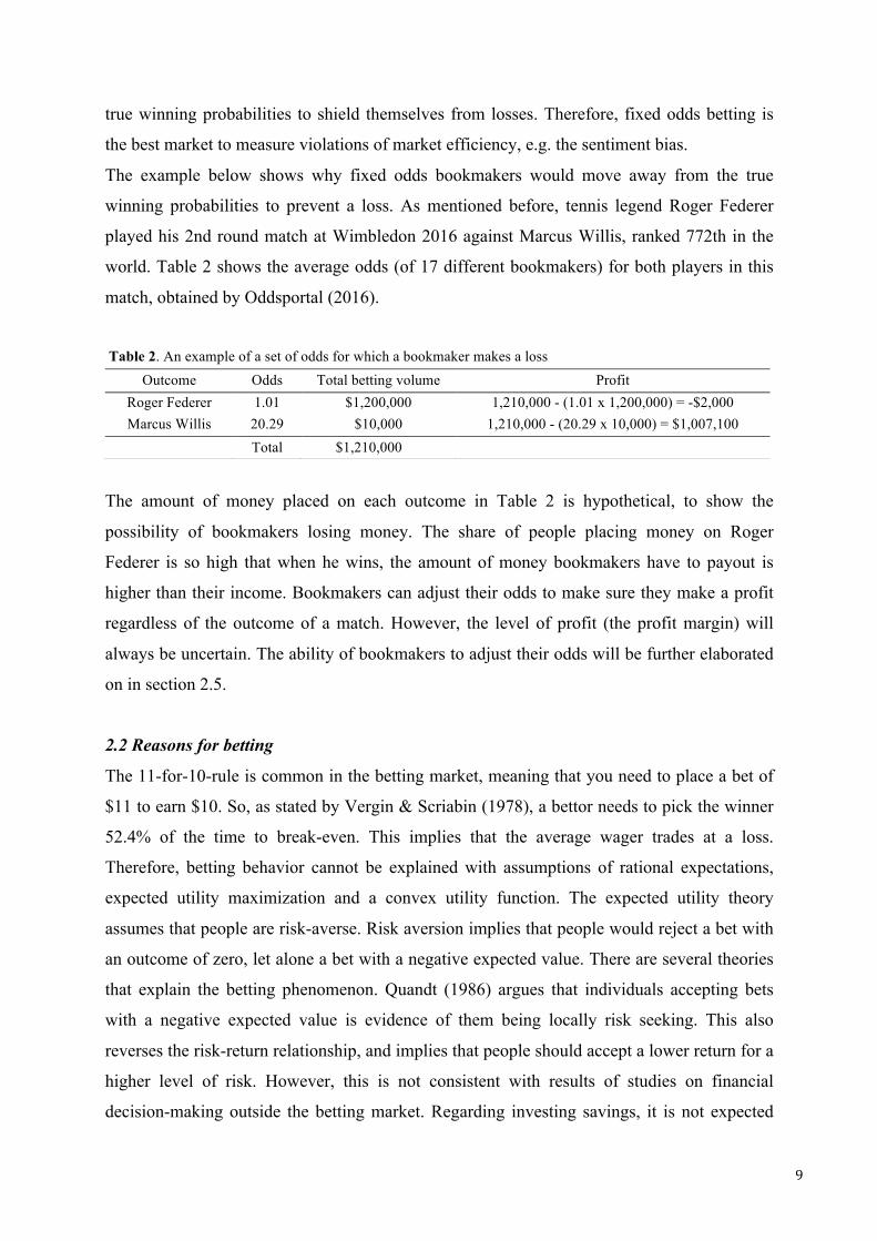
The example below shows why fixed odds bookmakers would move away from the true
winning probabilities to prevent a loss. As mentioned before, tennis legend Roger Federer
played his 2nd round match at Wimbledon 2016 against Marcus Willis, ranked 772th in the
world. Table 2 shows the average odds (of 17 different bookmakers) for both players in this
match, obtained by Oddsportal (2016).
Table 2. An example of a set of odds for which a bookmaker makes a loss
The amount of money placed on each outcome in Table 2 is hypothetical, to show the
possibility of bookmakers losing money. The share of people placing money on Roger
Federer is so high that when he wins, the amount of money bookmakers have to payout is
higher than their income. Bookmakers can adjust their odds to make sure they make a profit
regardless of the outcome of a match. However, the level of profit (the profit margin) will
always be uncertain. The ability of bookmakers to adjust their odds will be further elaborated
on in section 2.5.
2.2 Reasons for betting
The 11-for-10-rule is common in the betting market, meaning that you need to place a bet of
$11 to earn $10. So, as stated by Vergin & Scriabin (1978), a bettor needs to pick the winner
52.4% of the time to break-even. This implies that the average wager trades at a loss.
Therefore, betting behavior cannot be explained with assumptions of rational expectations,
expected utility maximization and a convex utility function. The expected utility theory
assumes that people are risk-averse. Risk aversion implies that people would reject a bet with
an outcome of zero, let alone a bet with a negative expected value. There are several theories
that explain the betting phenomenon. Quandt (1986) argues that individuals accepting bets
with a negative expected value is evidence of them being locally risk seeking. This also
reverses the risk-return relationship, and implies that people should accept a lower return for a
higher level of risk. However, this is not consistent with results of studies on financial
decision-making outside the betting market. Regarding investing savings, it is not expected
Outcome Odds Total betting volume Profit Roger Federer 1.01 $1,200,000 1,210,000 - (1.01 x 1,200,000) = -$2,000 Marcus Willis 20.29 $10,000 1,210,000 - (20.29 x 10,000) = $1,007,100
Total $1,210,000

10
that people accept a lower return for a higher level of risk. There are several theories to
explain this inconsistency.
According to Thaler and Ziemba (1988), the fact that bettors are risk seeking should be
explained by the characteristics of betting. In other words, "the term "locally risk seeking"
may apply to racetrack bettors, but only if the term "locally" refers to physical location rather
than wealth level" (p. 170). In case of racetrack betting, this refers to the local track where
bettors place their bets. The atmosphere of the racetrack, fans, fellow bettors and the
excitement for the race might turn people into risk-seeking bettors. Decisions on retirement
savings have different characteristics, and do not elicit this excitement to place a risk-seeking
bet and are therefore treated with a risk-averse attitude.
A second explanation is the mental accounting theory by Thaler (1985) He defines mental
accounting as "the set of cognitive operations used by individuals and households to organize,
evaluate and keep track of financial activities" (Thaler, 1999, p.183). People have separate
accounts for current and future assets and act as if the assets in these groups are not fungible.
They obtain a different level of utility from each separate account, which affects the way they
invest the money (Thaler & Ziemba, 1988). The fact that individuals have a mental "betting
account" that they treat so differently compared with other assets can be further explained by
one of the pillars of mental accounting: prospect theory (Kahnemahn & Tversky, 1979). In
this theory, value is assigned to gains and losses relative to some reference point, rather than
the final value of assets. One of the characteristics of this s-shaped value function is that the
gain function is concave and the loss function is convex. In other words, individuals are risk
seeking for losses. This explains why individuals accept bets in the first place, as on average
they trade at a loss. Second, it clarifies why someone who lost money in a bet on a tennis
match will not quit betting. The loss of money increases the tendency to make up for the loss
by placing additional risk-seeking bets.
Conlisk's (1993) "utility of gambling"-model is a third explanation of the inconsistency in
how people treat different type of bets. He argues that people are risk-neutral in small
distances from their reference point. In small-risk gambles likes sports betting, wagers only
need a small push to move from risk-neutral to risk-seeking behavior. Conlisk (1993) defines
this small push as the utility of gambling. He adds this element to the expected utility theory
model, which makes it applicable to all types of gambles. In bets like buying fire insurance or
investing retirement savings, the utility of gambling term might be lower than the risk-
aversion term from the expected utility function. The same person might place a risk-seeking

11
bet on his favorite boxing player because the utility of gambling term exceeds the risk-
aversion term for this type of bet.
2.3 Types of bettors
The previous section explained why individuals engage in betting. In the decision stage of
whether someone places a bet or not, all participants in the betting market are similar and
assumed to be risk loving. However, once individuals have entered the betting market, the
betting behavior among wagers may differ significantly. Makropoulou and Markellos (2011)
explain this in their heterogeneous betting market model. The authors distinguish between
three types of bettors, categorized by the extent to which they are informed about the match
outcome.
First of all, noise bettors place their bet without it being based on any kind of objective
information regarding the match. Sentimental bettors, who place a bet based on the degree of
sentiment for a player, fall into this category as well. The fact that a player has high sentiment
does not automatically imply that he is the favorite to win the match, so this information is not
necessarily relevant for the objective probability of the match outcome. Forrest and McHale
(2007) argue that tennis will not be subject to sentiment traders because tennis is a specialized
betting field. However, almost ten years later, the media extensively covers tennis and all
necessary information about odds, matches and players is easily accessible on the Internet.
The second type of bettors is defined as informed bettors. They collect and exploit public
information about the match and the players, and make a betting decision based on that
afterwards. As will be explained later, bookmakers fall into this category as well
(Makropoulou & Markellos, 2011). They collect public information about bettors’ behavior
and set the odds accordingly.
The final category of bettors is called insiders. They bet on private information, which is
unknown to the other market participants, including the bookmaker. Match fixing, which falls
under insider trading, is a serious problem in tennis. This is the result of the fact that half of
the prize money is paid to 1% of the tennis players, which makes it attractive for, especially
lower-ranked, players to engage in match-fixing. There is even evidence that a former Grand
Slam winner lost matches in obscure circumstances (The Economist, 2016).

12
2.4 Market efficiency in the betting market
2.4.1 The Efficient Market Hypothesis
This study examines the market efficiency of the online tennis betting market. The Efficient
Market Hypothesis (EMH) assumes a market to be efficient if asset prices reflect all available
information in the market. In terms of betting markets, efficiency is reached when bookmaker
odds are an unbiased predictor of the match outcome. Previous literature on market efficiency
in betting markets distinguishes between two types of market efficiency. First, a betting
market is considered to be weak efficient if "the odds are sufficiently reflective of objective
probabilities so that no strategy exists that would give bettors a positive expected return"
(Forrest & Simmons, 2008, p. 119). This is known as the broad view. A betting market is
strong efficient if "the odds are sufficiently reflective of objective probabilities so that no
strategy exists that would improve on the (negative) expected return from betting randomly"
(Forrest & Simmons, 2008, p. 119). This is known as the narrow view. The definition implies
that the expected loss from a betting strategy should be equal to the bookmaker's take out
(Gray & Gray, 1997). If the loss from a betting strategy is smaller than the bookmaker's take
out, it means that a part of the bookmaker's commission is compensated by a profitable
strategy. This would improve the expected return from placing a random bet and violates
strong efficiency.
2.4.2 The sentiment bias
The existence of behavioral biases in the sports betting market is a violation of market
efficiency, because the odds reflecting the match outcome are biased. The competitive price
deviates from the true winning probability. This study tests for the sentiment bias, which
occurs when beliefs are based on heuristics rather than rational expectations. In turn, this
creates inefficient prices. In terms of this research, this implies that if there is sentiment bias
in the market for tennis, the odds are influenced by the degree of sentiment for a player,
measured by their popularity on Google Trends. In that case, individuals overstate the
probability the high-sentiment player wins the match (Kuypers, 2000). Avery and Chevalier
(1999) distinguish between two types of sentiment: anticipated and unanticipated. Anticipated
sentiment and the corresponding shift in demand for bets can be predicted in advance of
setting the odds. On the other hand, unanticipated sentiment appears during the period of
betting. In this case, the unanticipated effect "will lead to an observable trend in prices
whenever it distorts the equilibrium price from the true expected value of the asset" (Avery &
Chevalier, 1999, p. 496).

13
The sentiment bias can be explained by three (behavioral) phenomena: the availability bias,
the loyalty bias and the fact that people enjoy being entertained. First of all, "one may
estimate probability by assessing availability, associative distance" (Tversky & Kahneman,
1973, p. 163). As a result of the availability bias, individuals place bets on players with the
shortest associative distance. Players with high sentimental value are covered in the media
relatively often. In terms of this research, this means that these players have a high score on
Google Trends. Players with high sentiment are easily retrieved and this makes bettors
overstate the probability of this player winning the match.
Another explanation of sentimental noise traders is the loyalty bias, which keeps bettors from
betting against their 'own' team (Braun & Kvasnicka, 2013). Massey, Simmons and Armor
(2011) define the loyalty bias as the desirability bias, which means that predictions about
match outcomes are optimistically biased if people have a strong preference for a player or
team. This may refer to the observation that people tend to over bet on their home and
national team (Gandar, Zuber & Lamb, 2001). In tennis, these two biases play less of a role
because it is an individual sport and matches are played all over the globe. Players might play
a tournament in their home country once a year, but they do not have their own stadium where
they play every other week. Therefore, in tennis, the loyalty bias refers to bettors that have
sentiment for a player for reasons other than nationality or residence. This might be a player's
style, his appearance or his off-court activities. As a result of these loyalty-eliciting factors,
fans do not want to bet against that player. Massey, Simmons and Armor (2011) found that
even when people learn from their betting experience throughout a season, the optimism bias
persists. This theory explains why people keep placing optimistic bets on a player with high
sentiment, even though they know about the high risk of losing money.
Third, the sentiment bias is explained by the fact that people enjoy entertainment. Flepp,
Nüesch and Franck (2016) showed that betting volumes are strongly biased towards over 2.5
goals-bets. "Cheering for an exciting high-scoring match is more attractive than cheering for a
dull low-scoring match and the entertainment value is therefore certainly higher for the over
2.5 goals bet than for the under 2.5 goals bet. Hence, at least part of the betting volume
wagered on the over bet is expected to be sentimentally driven due to this preference" (p. 5).
This can be applied to tennis betting as well, where high sentiment players are expected to
play a match with a high entertainment value.

14
2.4.3 The favorite-longshot bias
The most robust behavioral bias in betting markets is the favorite-longshot bias. Cain et al.
(2000) define it as the bias where “favorites win more often than the subjective market
probabilities imply, and long shots less often” (p.25). In other words, the odds are out of line
with the objective market probabilities as bettors over bet on outsiders and under bet on
favorites.
The favorite-longshot bias has four behavioral causes. According to Thaler and Ziemba
(1988), individuals overestimate the probability that outsiders will win the match. In
calculating the utility of placing a bet, they overweight the small probability that the outsider
wins the match. Second, bettors may derive utility from placing a bet on the outsider; they
enjoy the risk-loving feature of holding a long shot ticket (Thaler & Ziemba, 1988). Third,
Golec and Tamarkin (1998) explain the favorite-longshot bias by the fact that people are
skewness loving. Long shot bets have a low return and high variance, both unattractive
features. However, the skewness of a long-shot bet compensates for these two factors. The
fourth explanation argues that bettors discount a fixed fraction of their losses (Henery, 1985).
This makes them underweight losses and overweight gains in their evaluation of a longshot
bet.
In case of a favorite-longshot bias, bookmakers underestimate the probability that the favorite
wins. If the high-sentiment player is also the favorite to win the match, the sentiment bias and
the favorite-longshot bias work in the same direction. In case of reversed sentiment bias,
when bookmakers overestimate the probability of the high-sentiment player, the two effects
work in the opposite direction. Therefore it is important to control for the favorite-longshot
bias when doing research on any other behavioral bias in betting markets.
2.5 The role of bookmakers
Shin (1991) was the first to state the importance of the supply side in explaining the sentiment
bias. As displayed in Table 2, it could be the case that bookmakers make a loss for a certain
outcome of a match. However, bookmakers can adjust their odds to change their income and
ensure a profit. According to the Levitt's model (2004), bookmakers can choose from three
profitable pricing strategies.
2.5.1 Balance the books
First of all, bookmakers can decide to balance the books. In this model, bookmakers play a
passive role in setting odds. In terms of the earlier example, this basically means that if bettors

15
bet heavily on Roger Federer, the bookmaker will increase the price (lower odds) on Roger
Federer and reduce the price (increase odds) on Marcus Willis, to induce more betting on the
latter. They will continue doing this until the prices equalize the quantity of money placed on
each side. The balancing strategy reduces the bookmaker's risk, because the eventual payout
will be the same whoever wins the match. Therefore, bookmakers who balance their books
are considered as risk averse (Avery & Chevalier, 1999). With balancing the books,
bookmakers do not need any skill in forecasting the outcome of the match. They only have to
be able to predict bettor behavior. If fixed odds bookmakers use this strategy, they act as
bookmakers in a pari-mutuel betting market because the strategy results in a fixed profit
margin (Forrest & Simmons, 2008). Note that the odds that bookmakers set when they
balance the books are not the efficient market prices, since they do not reflect the true
outcome probability of the match.
2.5.2 Set the market-clearing price
It is unrealistic that all bookmakers fully adjust their odds to the point where the books are
balanced. The second pricing strategy for bookmakers is to set the odds according to their
prediction of the true match outcome (Flepp et al., 2016). Amongst others, Forrest, Goddard
and Simmons (2005) prove that this is feasible, as they found that bookmakers are at least as
good at predicting match outcomes as statistical models. When bookmakers set odds based on
the true outcome probability, the corresponding odds are called efficient because the price
reflects all available information about the match and its players (Humphreys, 2010). It is
different from the first strategy in the sense that with these odds, the amount of money placed
on each side of the bet is not necessarily equal. This strategy carries a higher risk because if it
turns out that wagers are actually better at predicting the match outcome, bookmakers will
lose money. On average, however, the bookmakers will earn a fixed profit equal to the
commission. Bookmakers may opt for this strategy in case of very price sensitive bettors
(Flepp et al., 2016). If bookmakers increase the price on a popular bet too much, sentimental
traders switch to another bookmaker or do not place a bet at all. On the other hand, if they
decrease the price on a high sentiment bet below the true outcome price, the betting volume
on that bet increases but the bookmakers run a higher risk of losing money. To summarize,
there is a limit to what extent bookmakers can deviate from the true outcome probability.
Within this limit, however, they will deviate from the true winning probabilities in order to
rationally exploit bettor preferences. This is discussed in the next section.

16
2.5.3 Active odds setting
The third and final pricing strategy for bookmakers is to actively set odds, which is to
strategically deviate from the true outcome probability to exploit bettor preferences and
achieve higher profits. In terms of Levitt's (2004) model, it is applied when bookmakers are
better than bettors at predicting the match outcome and when they are able to predict betting
behavior. Makropoulou and Markellos (2011) offer a competing explanation, where active
odd setting can be explained as “the optimal pricing response of bookmakers to information
uncertainty” (p. 521). Individual betting behavior is public information for bookmakers, and
they set their odds accordingly. However, because noise traders bet randomly, there is always
a minimal level of uncertainty regarding the direction of future bets. In their view, the
adjustment of odds in the direction of the expected bias is a correction for this uncertainty.
Bookmakers run more risk by actively setting their odds. As a result of the risk-return
relationship, moving from efficient to inefficient odds will increase their expected profits
(Kuypers, 2000). If bookmakers decide to actively set their odds, there are two strategies on
how to make it profitable for them. If they know that people prefer to bet on players with high
sentiment, they can either increase or decrease the prices for the high-sentiment bet.
In the first case, they adjust the odds by offering less favorable prices (lower odds) for high-
sentiment players. In other words, they skew the odds against the player with the relatively
high sentiment. By doing this, the bookmaker takes advantage of the bettors' preference by
increasing the price on the most popular bet (Levitt, 2004). Put differently, it is price
discrimination to take advantage of sentimental bettors. Bookmakers only engage in this
shading of odds when placing a bet on the high sentiment player is less likely to pay off for
the bettors, holding the odds constant (Humphreys, 2010). Otherwise, increasing the price for
high-sentiment players would lead to a higher pay out for bookmakers. If bookmakers cross
this line, well-informed bettors who know the correct probability can earn a positive return by
combining bets at different bookmakers.
On the other hand, bookmakers can decrease the price for the high-sentiment bet. Rather than
punishing the loyal bettors by letting them pay a higher price, they try to induce more people
to bet on this player. The increased betting volume compensates for the lower price bettors
pay per unit bet, in terms of revenue. But, as mentioned before, the increased betting volume
will increase the payout in case the high-sentiment player or team wins the match.
According to Australia Sports Betting (2016), there is an arbitrage opportunity if the sum of
the best available inversed odds is less than 1. Because odds across bookmakers are highly
correlated, which will be proven with data from the tennis betting market, arbitrage

17
opportunities are limited. This is positive for bookmakers, as "the presence of small numbers
of bettors whose skills allow them to achieve positive expected profits could prove financially
disastrous to the bookmakers" (Levitt, 2004, p. 224).
3 Literature review
In 1999, Avery and Chevalier were the first to document the effect of investor sentiment on
the betting market. They examine the hypothesis that bettors on NFL matches between 1976
and 1994 bet on sentiment, rather than on the probabilities posted by the bookmakers. They
use three sentiment measures to account for the investor sentiment: expert opinions, a
measure of how well teams performed in the past two weeks (hot-hand bias) and a measure of
a team's past-year performance (prestige bias). They find that investors bet in the same
direction as all these sentiment measures. Bookmakers go in the opposite direction and offer
less generous point spreads for NFL teams with the highest sentiment. In other words,
bookmakers rationally exploit the bettor preferences. This is negative for the sentimental
bettors, as they have to pay a higher price to place a bet. However, the strategy to exploit this
bias, to bet on the relatively cheap low-sentiment player, is only "borderline profitable"
(Avery & Chevalier, 1999, p520), depending on the time period. In their late (early) period
subsample, the success rate of this betting strategy is 54% (50.5%), while a wager strategy
must have a winning ratio of 52.4% to be profitable, taking the bookmaker's commission into
account.
Strumpf (2003) also found that bookmakers shade prices against teams that receive a large
fraction of sentimental bets. He studied the sentiment bias using data on football, basketball,
baseball and ice hockey matches from illegal bookmakers in New York City. By using the
betting history of individual bettors, he elicited their bettor preferences. For example, he
assumed a bettor to be New York Yankees loyalist if he bet in favor of the Yankees 90% of
the bets involving the Yankees. He finds that bookmakers offer these sentimental bettors
unfavorable betting prices, explained by the fact that these loyal wagers have a higher
willingness to pay for a bet involving the team with the high sentiment.
Hong and Skiena (2010) built on the research of Avery and Chavelier (1999) by studying the
sentiment bias in the betting market of NFL matches. Their approach is different from the rest
of the studies. The authors look at the sentiment bias on match level rather than finding the
aggregate direction (positive or negative) of the mispricing. Their measure of sentiment is the
public opinion of teams, expressed in blogs and social media. This is computed by the
analytics system Lydia, which counts the number of positive and negative words about a

18
team. If, for a given match, the predicted point spread is higher (lower) than the real point
spread, a bet is placed on the underdog (favorite) team. Using this strategy for 30 bets per
year during their late-period subsample (2006-2009) identified the winner 60% of the time (as
predicted by the sentiment measure). This is a profitable strategy, as their required success
rate including the bookmaker's commission is only 53%. However, the small amount of data
raises concerns about the robustness of this study.
Forrest and Simmons (2008) were the first to document bookmakers who shade prices in
favor of bettors of high-sentiment teams. They studied the betting market of Spanish soccer
during the period of 2001-2005 and concluded that more favorable odds were offered to bets
on clubs with higher sentiment. This is positive for sentimental wagers, as it becomes cheaper
to place a bet on the team with higher sentiment. The result is obtained by means of a
multivariate model with the bookmaker's probabilities, the sentiment measure and a variable
to control for home bias. The sentiment measure used is the difference in home attendance in
the stadiums between the two teams, a proxy to measure the active fan base. Forrest and
Simmons (2008) contribute to the literature by determining the monetary value of two
possible strategies to exploit the positive sentiment bias. The first strategy is to place a one-
unit bet when the sentiment measure is larger than a certain threshold. This results in a loss
between -5.7% and -8.9%, depending on the threshold. Even though the strategy results in a
smaller loss than when betting randomly (approximately -16%), the sentiment bias is not high
enough to compensate for the bookmaker’s commission. The second strategy is to place a
one-unit bet when the difference between the win probability forecasted by the model and the
bookmaker's probability exceeds a certain threshold. Returns lie between -10.6% and +12.8%,
depending on the threshold. In other words, when the gap is large enough, this strategy is
profitable. Forrest and Simmons (2008) perform a robustness check by repeating their study
for data on matches in the Scottish soccer league between 2001 and 2005. Opposed to the
results in the Spanish soccer league, they find neither a home bias nor a favorite-longshot
bias. However, the results for the sentiment bias in betting prices are similar, the effect of a
team's sentiment on the probability of winning a bet on that team is positive and significant.
This strengthens their main results and the conclusion that bookmakers adjust the odds in
favor of bettors of high-sentiment clubs.
Research by Franck, Verbeek and Nüesch (2011) concerns the sentiment bias in the betting
market for English soccer matches between 2000-2008 and can be considered as a robustness
check for the study by Forrest and Simons (2008). They use a similar measure to proxy for the
sentiment of home and away teams, "taking the difference between their standardized mean
19
home attendances in the previous season" (Franck et al., 2011, p.510). Franck et al. (2011)
predict the outcome of a bet with the bookmaker's implied probabilities, the sentiment
measure and a control variable for the home bias. The results run parallel with Forrest and
Simmons (2008). Franck et al. (2011) find that more favorable bets are offered to wagers on
clubs with a larger number of supporters. In other words, the betting prices on the market for
English soccer are cheaper for bets on high-sentiment teams. In addition, this study examined
the difference of the sentiment bias between weekdays and weekends. Bookmakers decrease
prices (increase odds) for popular teams even more when wagers face lower opportunity costs
to follow the match and place a bet. Put differently, the market inefficiency is larger during
weekends.
Feddersen, Humphreys and Soebbing (2013) find positive sentiment bias in the betting prices
for NBA matches between 1981 and 2012. In this extensive dataset, they look for the
presence of sentimental investors by measuring the difference between the average arena
capacity utilization of the home and away teams in the previous year. An OLS model
explaining variation in point spreads shows that favorable point spreads are offered for games
involving teams with a high sentiment measure. Additional analysis in the form of a probit
model explains the variation in bet outcomes. It shows that the higher the difference in arena
utilization between home and away teams, the higher the probability that a bet on the home
team wins. Put differently, bookmakers underestimate the probability that teams with high
arena utilization, considered as popular, win. However, the effect is only less than 0.1%,
which is not enough to exploit the sentiment bias when the bookmaker's commission is taken
into account. The authors obtain similar results in a robustness check, where they use the
difference in the share of All Star votes for the two competing teams as a sentiment measure.
When the difference in the share of All Star votes increases, the spread is more in favor of the
popular team. In other words, bookmakers underestimate the spread for teams with a lot of
All Star votes. However, the effect is again not strong enough to compensate for the
bookmaker take out. This supports their earlier conclusion that "point spread shading cannot
be exploited as a profitable strategy" (p.19).
Flepp et al. (2016) examine the influence of sentiment betting on bookmaker pricing in
over/under 2.5 goals bets, for matches in 220 different soccer leagues. They are the first to use
betting volume as a measure for betting behavior. The over-2.5 goals bet is considered as the
high-sentiment bet, because this implies a match with a high entertainment value. Analysis
finds evidence for sentiment bias, i.e. 80% of betting volume is placed on the high-sentiment
bet. However, this imbalance in betting volume does not affect the betting prices and bettor

20
returns. Put differently, bookmaker prices do not deviate from the true outcome probability.
The authors argue that this is the result of price transparency among different bookmakers,
which make bettors price sensitive and prevents bookmakers from actively setting odds to
exploit sentimental preferences.
Table 3. An overview of the most important studies regarding the sentiment bias
Year Authors Subject Method Conclusion 1999 Avery and
Chevalier
Sentiment bias in the National
Football League, measured by
expert opinions and past
performance.
OLS &
Probit model
Reversed sentiment bias which
leads to a profitable betting
strategy.
2003 Strumpf Sentiment bias in the illegal betting
market for baseball, football, ice
hockey and basketball, measured by
team loyalty in betting behavior of
individual bettors.
OLS Reversed sentiment bias.
2008 Forrest and
Simmons
Sentiment bias in the betting market
for the Spanish soccer league,
measured by the difference in home
attendance between home and away
team.
Probit model Positive sentiment bias, which
leads to a profitable betting
strategy with a return of 12.8%.
The robustness check with data
from the Scottish soccer league
leads to similar results.
2010 Hong and
Skiena
Sentiment bias measured on match-
level in the National Football
League, proxied by the public
opinion of teams.
OLS The profitable strategy to exploit
this bias identifies the winner
60% of the time, where the
required success rate is only 54%.
2011 Franck,
Verbeek
and Nüesch
Sentiment bias in the betting market
for the English soccer league.
Probit model Positive sentiment bias, which is
larger during the weekends.
2013 Feddersen,
Humphreys
and
Soebbing
Sentiment bias in the betting market
for National Basketball Assocation
matches, measured by the difference
in arena capacity utilization between
home and away teams.
OLS
Probit model
Positive sentiment bias. The
srategy to exloit this bias is not
profitable.
2016 Flepp,
Nüesch and
Franck
Sentiment bias in the soccer betting
market for over/under 2.5 goals
bets, determined by betting
volumes.
Two-stage
least squares
model
Positive sentiment bias, which
does not lead to extremely high or
low bettor returns.

21
In summary, previous research has studied the sentiment bias in betting markets for soccer,
American football, basketball, baseball and ice hockey. Table 3 presents an overview of the
most important studies on the sentiment bias in sports betting. The main conclusion is that the
ambiguous results emphasize the need for additional research on this topic. The current study
contributes to the literature by focusing on the sentiment bias in the betting market for Grand
Slam tennis matches. The results will serve as new proof in the discussion of whether, and in
which direction, bookmakers distort their odds to exploit the sentiment preferences among
bettors.
4. Hypotheses
Previous literature in behavioral economics found evidence for violations of market efficiency
in financial markets. The same applies to betting markets, which are subject to various
behavioral biases. Foremost, evidence on the favorite-longshot bias has led to the rejection of
the hypothesis that bookmakers' odds in the tennis betting market include all public available
information (Forrest & McHale, 2007). More recently, researchers have been studying the
sentiment bias in various sports betting markets and found mixed but significant results.
Avery & Chevalier (1999) and Strumpf (2003) found a reversed pricing reaction on sentiment
bias in the NFL and the illegal betting markets for several American sports, respectively. This
means that bookmakers offer less favorable odds to bettors of popular teams. Ever since,
studies have only found evidence for the opposite price shading: bookmakers offer more
favorable odds to bettors of popular teams. Returns of backing the high-sentiment player (or
team) have therefore been abnormally high. These results are robust for betting on matches in
the NBA (Feddersen et al., 2013), the NFL (Hong & Skiena, 2010), the English (Franck et al.,
2011) and Spanish soccer leagues (Forrest & Simmons, 2008). As this is a wide variety of
betting markets, it is expected to find similar results for the tennis betting market. The
sentiment measure used is data from Google Trends. It is expected that the higher the Google
Trends score for a player, the lower the prices that are offered for bets on these players. To
summarize, previous results and theories lead to the expectation that the market for tennis
betting is inefficient:
Hypothesis 1: Bookmakers underestimate winning probabilities for high-sentiment players,
whereas they overestimate winning probabilities for players with low sentiment.

22
Grand Slam tournaments are played over the course of two weeks. The final is played on the
second Sunday. In finals, odds are expected to lie closer to each other than for matches in the
first rounds of the tournament. As a result, the difference in the sentiment measure between
both between players will be relatively small as well. However, this implies that high ranked,
glamorous players with high sentiment are playing finals relatively often. Based on this, one
would expect that bookmakers deviate their odds further away from the true winning
probability. Independent of the characteristics of the players that reached the final, there is
another factor at work. In weekends, when finals are played, the fraction of noise bettors is
higher because of lower opportunity costs (Sung, Johnson & Highfield, 2009). As a result,
bettors are expected to be less price sensitive. These theories are strengthened by the result of
Franck et al. (2011), who report that the sentiment bias in soccer is higher during weekends.
As a result, it is expected that the level of sentiment has a stronger effect on the probability of
winning a bet in finals than in earlier rounds. This is summarized in the second hypothesis:
Hypothesis 2: The bookmaker's deviation from the true winning probabilities of high
sentiment players is larger during tournament finals than during earlier rounds.
The dataset in this research runs from 2004 until 2016, including the years in which the so-
called Big Four (Roger Federer, Rafael Nadal, Novak Djokovic and Andy Murray) dominated
the ATP World Tour. Together they have won 42 of the last 47 Grand Slam tournaments.
These players have become immensely popular over the years and are expected to elicit high
sentiment among noise traders. This sentiment might translate into loyal betting behavior, and
bookmakers are expected to exploit this lower price sensitivity. The imbalance between the
bookmaker probability and the predicted probability of the match outcome is expected to be
larger for matches of these players. The large number of observations ensures enough data
points for the Big Four sample to compare the two groups. All together, it is expected that the
sentiment bias is higher in matches with the Big Four. This is summarized in the third
hypothesis:
Hypothesis 3: The bookmaker's deviation from the true winning probabilities of high
sentiment players is larger in matches with the Big Four than in matches without the Big
Four.

23
Hypotheses 1 through 3 present the expectation of a positive sentiment bias, where
bookmakers underestimate the probability that popular players win. This implies that
bookmakers offer relatively cheap prices for bets on players with high sentiment. They know
that players with high sentiment are over bet and players with low sentiment are under bet.
Engaging in a strategy of placing a bet whenever the difference in the number of searches on
Google exceeds a certain threshold could result in a positive expected return. Forrest and
Simmons (2008) find that a betting strategy to exploit the positive sentiment bias in the
Spanish soccer league yields a profit of -5.7%, which is better than the return from random
betting. The same strategy is found to be profitable in betting on matches in the NFL (Hong &
Skiena, 2010). On the other hand, Feddersen et al. find a positive sentiment bias in the NBA
that cannot be profitably exploited by betting on the high sentiment players. The conflicting
results may depend on the variety of the bookmaker's commission in different betting
markets. The profitability of the strategy partly depends on this take out ratio because it is
subtracted from bettors' revenues. So even if the strategy provides positive revenue, it does
not have to be profitable. Forrest & McHale (2007) argue that the tennis betting market, on
average, has low transaction costs and well-informed bettors. These are both factors that work
as an advantage in exploiting the positive sentiment bias, if present. This, together with results
of previous studies, leads to the fourth hypothesis, which will be tested for each of the
samples used in Hypothesis 1 through 3:
Hypothesis 4: By engaging in a strategy of betting in favor of the high-sentiment player in
case of positive sentiment bias, and against the high-sentiment player in case of reversed
sentiment bias, bettors can earn a positive return.
5. Data
5.1 Betting data
Betting data for Grand Slam tournaments in the period 2004 - 2016 is collected from
www.tennis-data.co.uk. The first tournament in the dataset is the 2004 Australian Open and
the final tournament is the 2016 French Open. Different bookmakers offer different odds, and
wagers can choose where they want to place their bet. The dataset contains closing odds from
eight different bookmakers. Closing odds have the advantage of being adjusted for betting
volumes. Therefore, they represent the market prices of the bets on each player (Woodland &
24
Woodland, 1991). The initial dataset consists of 6350 matches, comprised of 127 matches in
each of the 50 tournaments.
5.2 Google Trends data
These 6350 matches contain 546 unique players. The sentiment for these players is measured
by Google Trends data. It is a service from Google to measure the popularity of search terms
over time. Data is available from 2004 onwards, which is the reason why the Australian Open
in 2004 is the first tournament in the dataset. When one enters a search term in Google
Trends, it shows the search popularity relative to the highest score of popularity, for that
search term, in the chosen time period. A value of 100 equals the peak popularity within the
time frame. A value of 50 means that at that time, the search term is half as popular as it was
on its peak. A score of 0 means that the search term has less than 1% popularity compared to
the peak. Google Trends data is measured on a weekly basis.
Google Trends has a function to compare two search terms with each other. This function is
important for the following reason. In order to be able to compare the sentiment for different
players, The Google Trends data for the 546 unique players need to have the same
normalization factor. This could have been realized by comparing the 546 search terms at
once. However, there is a maximum of entering five search terms in one session. To solve this
issue, all players have been compared, one by one, to the same player: José Acasuso. He is
chosen for the simple reason of being on top of the player list in alphabetical order. José
Acasuso’s popularity has been normalized against 545 different players. All matches with him
as either winner or loser have therefore been eliminated from the dataset.
Another important aspect of the data collected from Google Trends is the category in which
one searches. When entering the name of a tennis player in Google Trends, one can choose to
search for these words literally, or within the category of 'tennis player'. The first option gives
data on all searches for that name, regardless if it concerns the tennis player or someone else
with the same name. This is risky, since it might be the case that e.g. a singer has the same
name as a tennis player. Sentiment data on the singer would be included in the data that was
supposed to be on the tennis player only. In this research, therefore, data was only collected
when Google Trends recognized the player’s name as being a tennis player. Six players (and
the matches they play) have been removed from the sample because there was no data in
Google Trends. This is not expected to bias the results, since these six players are unknown
and low-ranked players. Furthermore, all observations that needed to be removed were first-
round matches. There are 64 first round matches in each tournament, so the removal of

25
several of these observations is not expected to influence the results. Altogether the sample
consists of 439 unique players.
After merging all individual reports, the weekly data is used to calculate the average
sentiment score in quarter q for player i: 𝑆!,!. The sentiment is measured on a quarterly basis
to spread the relatively high sentiment during Grand Slams and to include the sentiment
created in additional important tournaments like Masters and the World Tour Finals4. This
quarterly sentiment measure is merged with the betting data, on match level, as follows: for a
match during a tournament in quarter q, player i receives his sentiment score of quarter q-1:
𝑆!!!,!. This is done to ensure that the influence of sentiment for players on betting odds
during a tournament is measured in terms of sentiment created in the previous quarter of the
year. Otherwise, sentiment earned by a player because of reaching the final of Wimbledon is
included in the sentiment measure that determines bettor behavior for the first round of the
same player in the same Wimbledon tournament. Secondly, it is assumed that bettors and
bookmakers determine winning probabilities based on players' results and behavior in recent
tournaments, i.e. the previous quarter. These tournaments are easy to retrieve and will,
according to the availability bias, mainly influence the behavior of bookmakers and bettors.
As the Australian Open takes place in January, the chosen method implies that the sentiment
measure for the Australian Open is based on data from the final quarter of the previous year.
Even though no Grand Slam takes place in this quarter, it is an important part of the tennis
season including several Masters tournaments and the year-end ATP World Tour Finals
(considered as the unofficial World Championships). Betting data during the French Open,
played in June, is matched with data in the first quarter of the year and thus includes the
sentiment during the Australian Open. Wimbledon is officially split between two quarters
because it is played during the final week of June and the first week of July. However, all
observations during Wimbledon are seen as taking place in the third quarter, using sentiment
data from the second quarter. Thus, the French Open is included in the popularity measure
that influences betting decisions during Wimbledon. The US Open takes place during the first
two weeks of September, also in the third quarter. As such, sentiment data from the second
quarter is matched to US Open observations. The 2004 Australian Open is removed from the
sample since Google Trends data is available as of January 2004, so it is impossible to match
it with sentiment data from the previous quarter.
4 A full overview of the ATP (Assocation of Tennis Professionals) World Tour and its tournament categories is presented in Appendix A (ATP World Tour, 2017).

26
5.3 The final dataset
Betting data is collected from eight bookmakers. For the sake of consistency, the data analysis
in this research is performed with odds from only one bookmaker. Table 4 lists all
bookmakers and the number of missing observations in the dataset. There is large discrepancy
between the different bookmakers, with Centrebet, Interwetten and Unitbet being least
complete. Bet365 has the highest coverage, with unavailable odds for only 25 matches. Table 4. Number of missing observations for each bookmaker
Using the data from Bet365 as default is not expected to influence the reliability of the results.
Table 5 shows the correlation between the odds of the eight bookmakers. The correlation
between the set of odds from Bet365 and the other bookmakers is almost equal to 1. For some
pairs of bookmakers there is no overlapping data. In other words, there are no matches for
which betting odds are available for both bookmakers. Choosing Bet365 as the bookmaker
whose odds will be used for the analysis removes another 25 matches from the sample. The
total number of observations, with complete data for both players on Google Trends and
betting odds, is 6156 matches.
Table 5. Correlation between the different bookmakers
As mentioned in the theoretical chapter, bookmakers require bettors to pay a commission to
ensure that they make a profit. This commission is included in the odds set by Bet365 and
Bet365 Centrebet Expekt Interwetten Ladbrokes Pinnacles Stan James Unibet Bet365 1
Centrebet 0.983 1 Expekt 0.979 0.978 1
Interwetten 0.956 0.963 0.959 1 Ladbrokes 0.973 0.675 0.971 0.639 1 Pinnacles 0.977 0.942 0.952 0.862 0.974 1
Stan James 0.952 - 0.977 - 0.947 0.911 1 Unibet 0.989 0.970 0.983 - 0.984 0.973 0.925 1
Bookmaker Number of missing observations Bet365 25
Centrebet 4330 Expekt 38
Interwetten 5314 Ladbrokes 1767 Pinnacles 538
Stan James 3160 Unibet 4199

27
causes the sum of the odds (expressed as probabilities) to be higher than unity. The
'probabilities' of each player winning the match, including the commission, are calculated as
follows:
𝑝𝑟𝑜𝑏𝑐𝑜𝑚!,! =1
𝑜𝑑𝑑!,!
, with 𝑜𝑑𝑑!,! being the payout if one places a bet of 1$ on player i winning match m and
𝑝𝑟𝑜𝑏𝑐𝑜𝑚!,! being the 'probability' of player i winning match m. These probabilities in the
dataset need to be adjusted for the overround. The average overround of Bet365 in the dataset
is 6.61%. This means that in order to break-even, on average bettors need to win 51.60% of
their bets. In line with previous studies, it is assumed that the bookmaker’s commission is
equally distributed over the two outcome probabilities for a match (Franck et al., 2010). The
implied probabilities, which will then sum to 1 for both players, are calculated as follows:
𝑖𝑚𝑝𝑟𝑜𝑏𝑖,𝑚 = 𝑝𝑟𝑜𝑏𝑐𝑜𝑚𝑖,𝑚
𝑝𝑟𝑜𝑏𝑐𝑜𝑚𝑖,𝑚𝑖.
6. Methodology
6.1 The probit model
The multiple linear regression model with a binary dependent variable is called the linear
probability model (LPM) because the response probability is linear in the parameters. This
model is easy to estimate and interpret but it has two main drawbacks (Wooldridge, 2015).
First, the fitted probability predicted by LPM can be less than zero or greater than one.
Second, the LPM assumes constant marginal effect for an independent variable. For example,
the LPM would predict that the effect of a player going from none to one injury reduces the
probability of winning by the same amount as the player going from one to two injuries. The
probit model overcomes these shortcomings and is therefore used in this paper.
The probit model is a binary response model with a limited dependent variable for which the
range of values is restricted. In the curent study it is a binary variable that takes either value 1
or 0. The general probit model is formulated as follows:
𝑃(𝑦 = 1|𝕩) = 𝐺(𝛽! + 𝕩𝜷)
, where G is standard normal cumulative distributive function, expressed as an integral. 5
This study tests whether the market for tennis betting is subject to sentiment bias. If so, our
measure of sentiment has some explanatory power to the true winning probabilities. This
5 𝐺(𝑧) = Φ(𝑧) = 𝜙!
!! (𝑣) 𝑑𝑣 with Φ(𝑧) = (2𝜋)!!/!𝑒𝑥𝑝(− !!
!)

28
implies that there is market inefficiency, since the odds set by Bet365 do not contain all
publicly available information and deviate from the efficient level at which each bet is, on
average, equally profitable (Franck et al., 2011). The hypothesis is tested by estimation of the
following probit model:
𝑌! = 𝐺 𝛽! + 𝛽!𝐷𝐺𝑇! + 𝛽!𝑝𝑟𝑜𝑏! + 𝛽!ℎ𝑜𝑚𝑒! + 𝛽!ℎ𝑜𝑝𝑝! + 𝑢!
Yi is the binary dependent variable explaining the actual outcome of the bet, which equals 1
for a winning bet and 0 for a losing bet. The actual outcome of the bet is explained in terms of
four independent variables. 𝐷𝐺𝑇! is the proxy for sentiment and measures the difference in the
Google Trends score in the previous quarter between player i and his opponent. 𝑝𝑟𝑜𝑏! is the
implied bookmaker probability of a win for player i minus the implied bookmaker probability
for his opponent. This will show whether bookmakers give favorites enough, too much or too
little credits. It is important to note that this is not a control for the favorite-longshot bias, as
this variable does not tell anything about behavior of extreme favorites or underdogs in
particular. An extra analysis will be performed to provide evidence in favor or against the
favorite-longshot bias.
Bettors are known to over bet on home teams and therefore the model needs a control for the
home bias. If the home player is the player with the highest sentiment, the distortion in
probabilities might be related to the player playing at his home tournament rather than being
the most popular player. The inclusion of dummy variable ℎ𝑜𝑚𝑒! controls for these home
player bets. It has a value of 1 for the matches where player i plays at his home tournament,
and 0 otherwise. This concerns Australian players, French players, British players and
American players for the Australian Open, Roland Garros, Wimbledon and the US Open
respectively. A similar dummy variable is included to control for the home bias of the
opponent.
The probit model is symmetric because all variables for player i are measured relatively to its
opponent6. This ensures that the winning probabilities for a player and its opponent estimated
by the model sum to 1 for every match. Betting on a match is a zero-sum game, since a
winning bet on a player implies that the bettor on the other side loses. As a result,
observations are independent across matches but correlated within matches. The correlation of
the error terms violates the independence assumption. This is corrected for by clustering
observations within the same match. This method generates robust standard errors for the
6 The dummy variable indicating home tournaments is not measured relatively to the opponent. However, a dummy for the opponent's home matches is included to correct for this.

29
estimated coefficients. As a robustness check, the analysis is repeated with randomly
sampling one observation from each match instead of creating clusters. 7
6.2 Model estimation
The probit model is estimated by Maximum Likelihood Estimation (MLE). The main
advantage of this method is that "the general theory of MLE for random samples implies that,
under very general conditions, the MLE is consistent, asymptotically normal, and
asymptotically efficient" (Wooldridge, 2015, p. 588). The maximum likelihood estimator of 𝜷
is equal to 𝜷. If 𝐺(∙) is equal to the standard normal cumulative distribution function, 𝜷 is
called the probit estimator.
The magnitude of the estimated coefficients, 𝛽! , can not be interpreted because of the
nonlinear nature of 𝐺(∙) . To estimate the individual effect of 𝐷𝐺𝑇! , 𝑝𝑟𝑜𝑏! , ℎ𝑜𝑚𝑒! and
ℎ𝑜𝑝𝑝! on the probability of winning the bet, P(y = 1 | 𝕩), one needs to calculate the marginal
effects8: 𝛿 𝑝 𝑥𝛿 𝑥!
= 𝑔 𝛽! + 𝕩𝜷 𝛽!
The scale factor of the partial effect depends on the value of all independent variables, 𝕩. To
calculate the partial effect, 𝐷𝐺𝑇! and 𝑝𝑟𝑜𝑏! are replaced with their average value and the
home dummies are set equal to 0. This results into the partial effect at the average (PEA), the
marginal effect of xj for the average player in the sample. The average partial effect (APE) is
calculated as a robustness check. This measure first calculates the partial effects on individual
level before these individual marginal effects are averaged across the entire sample. The
partial effect of the independent variables on the probability of winning the bet depends on 𝕩
through 𝑔 𝛽! + 𝕩𝜷 . Therefore, the marginal effect always has the same sign as the
coefficient 𝛽! (Wooldridge, 2015).
Since the estimated coefficients have a robust standard error, the statistical significance of the
three independent variables can be tested with a two-tailed t-test. This test decides whether
the sentiment proxy, the home dummies and the bookmaker's implied probabilities have a
significant effect on the probability of winning a bet. If the null hypothesis is rejected, one can
conclude that the variable has a significant effect, implying market inefficiency.
7 The random sampling process has been repeated several times to ensure robust results. 8 𝑔(𝑧) = !"(!)
!"

30
6.3 Goodness-of-fit
The quality of the probit model will be evaluated with two goodness-of-fit measures. The first
one is McFadden's pseudo R-squared:
𝑅! = 1−ℒ!"ℒ!
ℒ!" is the log-likelihood function for the unrestricted probit model, including the four
independent variables. ℒ! is the log-likelihood function for the model with only an intercept.
If the model in this research has no explanatory power, these two log-likelihoods function are
equal to each other and the R2 equals zero. The goodness-of-fit of the estimated model
increases as McFadden's pseudo R2 moves closer to unity. It should be noted, however, that it
cannot be interpreted as the fraction of total variance explained by the model, the definition of
the normal R2. If you would put values for both measures in a diagram, it is not a straight line.
Higher values of the R2 are translated into lower values for McFadden's pseudo R2. Therefore,
values for the McFadden pseudo R2 of 0.2 and higher are considered a good fit.
The second goodness-of-fit measure determines how well the probit model predicts the Grand
Slam match results, compared with the bookmakers (Hvattum & Arntzen, 2010). A bet is
placed when the probability of a player winning the match predicted by the probit model,
multiplied by the Bet365 odds, is greater than one. These cases, defined as value bets, will be
evaluated by two betting strategies. The first one is called Unit Bet, with a fixed stake of 1$.
This will result into a gain of $odds - 1 in case the player wins, and a loss of -$1 if he loses.
The second strategy is called Unit Win, which has a betting size that results into a fixed gain
of 1$ if the player wins. If the player loses, the loss equals the stake. The advantage of the
Unit Win strategy is that it is less prone to heavy losses from bets that have high odds,
because the stakes are lower (Hvattum & Arntzen, 2010).
7. Results
7.1 Summary statistics
The summary statistics of the independent and dependent variables estimated in the probit
model are presented in Table 6. The mean value of the dependent variable, 𝑌!, is equal to 0.5,
explained by the fact that in tennis bets there is either a win or a loss. The sum of the implied
probability odds for two players in a match is always equal to one, such that the mean value
of the bet automatically equals 0.5. Franck et al. (2011) study the sentiment bias in soccer

31
matches and leave out draw bets. As a result, the implied probability odds sum up to less than
1, and the mean value is lower than 0.5.
The difference in sentiment value between two players has a mean value of zero. This is
explained by the fact that every match comprises of two observations, one for the winner and
one for the loser. The value of 𝐷𝐺𝑇! for the former is equal to the Google Trends score of the
winner minus the Google Trends score of the loser. This is opposite for the observations with
the loser as subject player. As a result, the average value is equal to 0. The maximum absolute
difference of sentiment between two players is equal to 42.538.
The same explanation applies to the symmetrical variable of the implied bookmaker
probability. The value of 𝑝𝑟𝑜𝑏! is determined by the implied winning probability for player i
minus the bookmaker probability his opponent wins. Since both the winner and the loser are
in the sample, the mean value of this variable is equal to 0. The maximum difference in
bookmaker probabilities between two players is 0.995, which implies that the sample contains
some very lopsided matches.
Table 6. Summary statistics
Table 6 shows negative correlation between the home dummy and the remaining variables.
The negative correlation coefficient for variable 𝑝𝑟𝑜𝑏! can be explained by the fact that Grand
Slam tournaments give the majority of their wildcards to home players whose ranking is not
high enough for direct qualification. Their low ranking is a reason for bookmakers to set a
low winning probability for these players, as they are obviously not the favorite to win the
match.
The correlation coefficient between the sentiment proxy and the bookmaker probabilities is
equal to 0.333. This implies that a higher difference in bookmaker probability between two
players is associated with an increase in the difference between the sentiment measures of
both players. Put differently, players that are considered as being the favorite may, on
average, also be the more popular player.
Variable Description Mean Standard Deviation Min Max 1 2 3 4 5
1 𝑌! Outcome of bet i 0.500 0.309 0.04 0.96 1.000 2 𝐷𝐺𝑇! Relative sentiment 0.000 7.228 -42.54 42.54 0.342 1.000 3 𝑝𝑟𝑜𝑏! Relative probability 0.000 0.558 -0.97 0.97 0.995 0.333 1.000 4 ℎ𝑜𝑚𝑒! Home player i 0.091 0.228 0.00 1.00 -0.025 -0.072 -0.041 1.000 5 ℎ𝑜𝑝𝑝! Home opponent 0.091 0.228 0.00 1.00 0.025 0.072 0.041 0.001 1.000

32
7.2 The full sample
7.2.1 Regression results
Table 7 presents the results of the clustered9 probit model that predicts the probability of
winning the bet on player i. The McFadden's pseudo-R2 is equal to 0.3091. Given the
distribution of this measure, the value implies that the probit model is a very well fit.The
value is higher than the McFadden pseudo R2 in similar models estimated by Franck et al.
(2011) and Forrest & Simmons (2008), 0.062 and 0.115 respectively.
The coefficients in Table 7 do not represent the magnitude of the effect of the independent
variables on the bet outcome. They do, however, reveal the significance and sign of the
variables. The second line in Table 7 displays that the variable 𝐷𝐺𝑇! has a p-value of 0.230,
which means that the null hypothesis of market efficiency in terms of sentiment cannot be
rejected. Put differently, the relative popularity of a player has no significant effect on the
outcome of a bet on that player. Bookmakers do not underestimate the winning probabilities
of high-sentiment players. The results are not in line with Hypothesis 1.
Table 7. Clustered probit regression results
Notes: The dependent variable is equal to the outcome of bet i. * = significant at 10% level, *** = significant at 1% level.
The difference in bookmaker probabilities between player i and his opponent has a significant
and positive effect on the actual outcome of a bet. With a t-statistic of 45.62 and a p-value of
0.000, the variable is individually significant at the 1% level. When the difference of implied
winning probabilities between the average player and his opponent increases by 10 percentage
points, the probability that a bet on the average player is won increases by 6.90%, ceteris
paribus.10 This marginal effect indicates that bookmakers give too much credit to favorites.
However, this result does not show whether the bookmaker changes his pricing strategy for
extreme probabilities in particular (extreme favorites and longshots). In order to properly
9 As a robustness check, the probit model was estimated with random sampling rather than clusters. The results are documented in Appendix B. 10 The Average Partial Effects (APE) have been calculated as a robustness check. The results are similar and documented in Appendix C.
Coefficient Marginal effect T-statistic P-value 𝐷𝐺𝑇! 0.003 0.001 1.20 0.230 𝑝𝑟𝑜𝑏! 1.73 0.690 45.62*** 0.000 ℎ𝑜𝑚𝑒! 0.077 0.031 1.69* 0.092 ℎ𝑜𝑝𝑝! -0.077 -0.031 -1.69* 0.092 Number of observations 12312 Number of clusters 6156 Pseudo - R2 0.3093
33
examine whether the favorite-longshot bias is present in this sample, one needs to look at the
behavior at different range of odds. An additional analysis, of which the results are
documented in Appendix D, examines whether the sign and magnitude of the effect changes
over the range of bookmaker probabilities for favorites.11 The results show that bookmakers
actually underestimate the winning probability for extreme favorites (implied bookmaker
probability > 0.75), which implies that bettors over bet long shots. This is in line with the
favorite-longshot bias.
The third explanatory variable is the dummy that indicates whether a player is playing a
match during his home tournament. With a t-statistic of 1.69 and a p-value of 0.092, this
variable is borderline significant at the 10% level. In other words, bookmakers underestimate
the probability that a bet on a home player is won. They offer relatively cheap prices for bets
on home players. The marginal effect in Table 7 reveals that the probability of winning the
bet on the average player is approximately 3.1% higher when it concerns a match at that
player's home tournament, ceteris paribus. The results for variable ℎ𝑜𝑝𝑝! are exactly opposite,
given the symmetric characteristics of the model. Bookmakers overestimate the winning
probability for a player of which the opponent plays a match in his home tournament.
7.2.2 Unit Bet and Unit Win
Table 8 displays the returns per dollar bet for the Unit Bet and Unit Win strategy. The Unit
Bet strategy has a return of -0.1254 per 1$ bet, whereas the Unit Win strategy has a positive
return of 0.7066 per 1$ bet. The large difference between the two is caused by the smaller bet
size in the Unit Win strategy. If a player has very high odds, and a higher chance to lose the
match, the stake that is lost if he indeed loses is very small. However, in the Unit Bet strategy,
the loss is equal to $1 every time a bet is lost.
Table 8. Profits for Unit Bet and Unit Win strategies
Bet size Total return Unit Bet 1.000 -0.1254 Unit Win 0.647 0.7066
7.3 Sentiment bias in tournament finals
The second question this research aims to answer is whether the bookmaker's response to
bettor sentiment is higher during tournament finals compared with the rest of the tournament.
Table 9 displays the results from the clustered probit model for two samples: finals and non-11 Prior to the extra analysis, a squared term of the relative bookmaker probabilities was added to the probit model to measure behavior around extreme probabilities. However, this was insignificant.

34
finals. The samples have 98 and 12214 observations, respectively. Even though the final
sample size is much smaller, the McFadden's pseudo-R2 for both estimations are similar. The
values of approximately 0.30 indicate that the model is a very good fit for both samples.
In the sample for tournament finals, the sentiment variable 𝐷𝐺𝑇! is significant at the 10%
level, with a p-value of 0.06. The sign of the coefficient is negative, which means that for bets
on tournament finals the probability of winning a bet on a player decreases the higher his
relative popularity. Put differently, bookmakers overestimate the probability that the high-
sentiment player wins. When the difference in the Google Trends score between a player and
its opponent increases by 1.00, the probability that a bet on the average player is won
decreases by 2%, ceteris paribus. This is in line with earlier results from Avery and Chevalier
(1999) and Strumpf (2003). There is no significant sentiment bias, either normal or reversed,
in the non-final sample. In other words, bookmakers do not deviate their odds from the true
winning probabilities. An unreported two-tailed t-test shows that the coefficients of 𝐷𝐺𝑇! in
the "Final" and the "Non-Final" samples are significantly different from each other at the 5%
level, with a p-value of 0.04. The sentiment bias is larger in the final sample than in the non-
final sample, even though it is in the reversed direction. The results are in line with
Hypothesis 2.
The difference of bookmaker winning probabilities between player i and his opponent has a
positive and significant effect on the probability of winning a bet on that player. The variable
is significant on the 1% level in both samples. In the final (non-final) sample, the probability
of winning a bet on the average player increases by 10.11% (6.89%) when the difference in
bookmaker probability for the average player and his opponent increases by 10 percentage
points, ceteris paribus. This implies that, in the final sample, favorites win more often than
you would expect from the odds. On the other hand, in the non-final sample, favorites win
less often than implied by the bookmaker odds. As mentioned previously, this does not allow
one to conclude anything on the favorite-longshot bias.
The home dummies for a player and its opponent are significant at the 10% level in the non-
final sample. The probability of winning a bet on player i increases (decreases) by 3.1% if he
(his opponent) plays a match in his home country, ceteris paribus.

35
Table 9. Clustered probit regression results Final and Non-final samples
Notes: The dependent variable is equal to the outcome of bet i. * = significant at 10% level, *** = significant at 1% level
7.4 Sentiment bias in matches of the Big Four
The third hypothesis concerns the difference in sentiment bias between very popular players,
the Big Four, and less popular players. Table 10 displays the estimations of the clustered
probit model for the sample containing Big Four matches, and the sample with the remaining
matches. The two samples have 1812 and 10500 observations, respectively. The McFadden's
pseudo R2 of 0.6421 indicates an extremely well fit for the Big Four sample.
Table 10. Clustered probit regression results Big-Four and Non-Big Four samples
Notes: The dependent variable is equal to the outcome of bet i. ** = significant at 5% level, *** = significant at 1% level.
Table 10 displays that 𝐷𝐺𝑇! for the Big Four sample is statistically significant at the 5% level.
The sign is negative, which implies that the larger the difference in Google Trends scores
between two players, the lower the probability that a bet on the high-sentiment player is won,
ceteris paribus. Put differently, bookmakers overestimate the probability that the high-
sentiment player wins. The marginal effect can be interpreted as follows: when the difference
in the Google Trends score between a player and its opponent increases by 1.00, the
probability that a bet on the average player is won decreases by 0.8%, ceteris paribus. The
sentiment measure is not significant in the sample for matches without any of the Big Four
players. In other words, bookmaker probabilities do not under or over estimate the probability
that the high-sentiment player wins. An unreported two-tailed t-test confirms that the
Coefficient Marginal effect T-statistic P-value Final Other Final Other Final Other Final Other
𝐷𝐺𝑇! -0.050 0.003 -0.020 0.001 -1.88* 1.34 0.060 0.179 𝑝𝑟𝑜𝑏! 2.53 1.728 1.011 0.689 4.11*** 45.47*** 0.000 0.000 ℎ𝑜𝑚𝑒! 0.006 0.078 0.003 0.031 0.01 1.69* 0.993 0.091 ℎ𝑜𝑝𝑝! -0.006 -0.078 -0.003 -0.031 -0.01 -1.69* 0.993 0.091 Observations 98 12214 Clusters 49 6107 Pseudo - R2 0.3095 0.3097
Coefficient Marginal effect T-statistic P-value Big 4 Other Big 4 Other Big 4 Other Big 4 Other
𝐷𝐺𝑇! -0.021 0.004 -0.008 0.002 -2.33** 1.30 0.020 0.194 𝑝𝑟𝑜𝑏! 2.272 1.650 0.907 0.658 19.31*** 39.43*** 0.000 0.000 ℎ𝑜𝑚𝑒! -0.207 0.095 -0.082 0.038 -1.47 1.98** 0.142 0.048 ℎ𝑜𝑝𝑝! 0.207 -0.095 0.082 -0.038 1.47 -1.98** 0.142 0.048 Observations 1812 10500 Clusters 906 5250 Pseudo - R2 0.6421 0.2555

36
coefficients of 𝐷𝐺𝑇! in the Big Four and the non Big Four samples are significantly different
from each other at the 1% level. The absolute value of the sentiment bias is larger in the big
four sample than in the other sample, even though it is reversed sentiment bias. This is in line
with Hypothesis 3.
The bookmaker probability is positive and highly significant at the 1% level for both samples.
To be more precise, the probability of winning the bet on the average player in the Big Four
(non Big Four) sample increases by 9.07% (6.58%) when the difference in the bookmaker's
implied probabilities between the average player and his opponent increases by 10 percentage
points, ceteris paribus. Since both marginal effects are lower than 1, favorites win less often
than you would expect based on the odds.
Finally, the dummy variables indicating whether it is a player's (and his opponent's) home
tournament is significant at the 5% level in the non Big Four sample. The marginal effect in
Table 10 displays that the probability of winning the bet on the average player increases by
3.8% when it concerns a match at that players' home tournament, ceteris paribus. This
indicates a positive home bias. Put differently, bookmakers underestimate the probability that
players win matches at their home tournament, given it is a match without any of the Big Four
players.
7.5 Exploiting the sentiment bias
The significance and sign of the sentiment bias determine the appropriate strategy to exploit
bookmaker's mispricing. These strategies are presented below, for each of the three samples:
the full sample, the tournament finals and the Big Four matches.
7.5.1 The full sample
In the full sample, the relative sentiment measure for a player has no significant quantitative
effect on the probability of winning a bet on that player. Bookmakers do not over or
underestimate the probability that high sentiment player win a match. There is market
efficiency in terms of sentiment, as the implied probabilities reflect the true winning
probabilities for both the winner and the loser. There is no possibility for well-informed
bettors to capitalize on the sentiment bias, because there is no pricing advantage for any type
of player. In terms of sentiment bias, the market for tennis betting is weakly and strongly
efficient. There is no strategy to improve on the return from random betting nor to earn a
positive return.
37
7.5.2 The tournament finals
The significant but reversed sentiment bias implies bookmakers overestimate the probability
that high-sentiment players win a match, given it is a tournament final. In other words, they
offer a relatively high price for bets on the high-sentiment player. This can be exploited by
placing a unit bet on the finalist with the relatively low sentiment. The return per unit bet for
this strategy is equal to -0.0280, or -2.80%. This is an improvement on the return of randomly
betting on each of the two players for all matches in this sample, which equals -25.51%. This
implies that the market for tennis betting in the sample for tournament finals is weakly
efficient but not strongly efficient. The return from betting randomly can be improved, but not
to an extent that there is a positive return. In other words, the revenues are not high enough to
compensate for the bookmaker commission.
7.5.3 The Big Four
The measure for relative sentiment of a player has a significant and negative effect on the
probability of winning a bet on that player, given it is a match starring any of the Big Four.
Bookmakers therefore overestimate the probability that the high-sentiment player wins the
match. In other words, they offer a relatively low price for betting on the low-sentiment
player. This could possibly be exploited by placing a unit bet on the low-sentiment player for
every match in the sample. The return for this strategy is equal to -35.76%. This is not an
improvement on the return from placing bets at random in this sample, which equals -27.30%.
Given that it is not possible to exploit the reversed sentiment bias by any means, the market
for betting on Big Four matches is weakly and strongly efficient. The negative return could be
the result of the low-sentiment player being very much the underdog compared to the high-
sentiment player (any member of the Big Four). So even though there is a relative pricing
advantage for low-sentiment players, this does not compensate for the fact that the high-
sentiment player is the big favorite to win the match.
8. Conclusion
The empirical evidence on the direction to which bookmakers shade prices, as a result of
bettor sentiment, is mixed. This study tested for market efficiency in the unexplored market of
tennis betting. It is a question of whether bookmakers under or overestimate the winning
probability for high-sentiment players in Grand Slam tournaments between 2004 and 2016.
The results contribute to the existing literature on the sentiment bias, being the first to
research data on tennis bets.

38
The full sample does not show any sentiment bias. Bookmakers do not under or overestimate
the winning probabilities for popular players. The absence of a sentiment bias in bookmaker
prices is in line with results of Forrest and McHale (2007), who argue that this is the result of
tennis being a specialized betting market. However, the results are not in line with recent
studies that found evidence for bookmakers actively setting odds in English and Spanish
soccer (Franck et al., 2011), the NBA (Feddersen et al., 2013) and the NFL (Hong & Skiena,
2010). An explanation of the result, bookmakers setting unbiased odds equal to the true
winning probabilities, is price sensitive bettors. This implies that tennis bettors are, on
average, not extremely loyal to their favorite players. If the price of a sentimental bet
increases to more than a certain threshold, they move to another bookmaker or do not place a
bet at all. This is why bookmakers prefer to play safe and do not shade prices in favor or
against high-sentiment players. All together, there is no evidence to accept Hypothesis 1.
Findings show that bookmakers overestimate the winning probabilities of high-sentiment
players in tournament finals. This result is in line with studies by Avery and Chevalier (1999)
and Strumpf (2003). The so-called reversed sentiment bias is significantly larger in
tournament finals than in earlier rounds. It implies that bookmakers shade prices against the
popular players in tournament finals, whereas they do not in earlier rounds. This is in line
with previous results from Franck et al. (2011), who found that the sentiment bias is amplified
during weekend bets on English soccer matches. There are two explanations for the difference
between the two subsamples. Bookmakers might expect bettors to have a higher level of
sentiment during finals, because if their favorite wins the match he wins the entire
tournament. This increased sentiment will keep them from refraining their bet in case of a
price increase. Put differently, the fact that bettors are less price-sensitive in tournament finals
allows the bookmaker to exploit the sentiment. Secondly, bookmakers might increase prices
for bets on high-sentiment players in tournament finals because they know that noise traders
have lower opportunity costs during the weekend, when finals are played. The results are in
line with Hypothesis 2.
Bookmakers also deviate from the unbiased odds in matches with any of the Big Four players.
They overestimate the winning probability for popular players, a fact that implies a bet on
these players is relatively expensive. Bookmakers do not shade prices for matches without
superstars, which is in line with Hypothesis 3. There are three reasons why bettors are less
price-sensitive in matches with these four players. The Big Four elicit more bettor sentiment
than any other high-sentiment player. These players have strong fan bases around the world,
which increases bettors' loyalty bias. People will extensively bet on Roger Federer until he
39
retires, even when he is the clear underdog, simply because he is so popular. Second, bettors
are confronted with these players in interviews, on posters, social media and TV commercials
on a daily basis. In other words, these players are easy to retrieve and they will more likely
place sentiment bets on these players because they are familiar with the names. This is an
effect of the availability bias. Third, people prefer matches with high entertainment value and
there is always something at stake for these players, especially at Grand Slams. Whether it is
Novak Djokovic completing his career Grand Slam, Andy Murray winning Wimbledon for
the first time, Roger Federer winning his 18th Grand Slam or Rafael Nadal winning Roland
Garros for the tenth time, history is always made. These are the reasons why bookmakers dare
to increase their prices for bets on Big Four players, but not for any other high-sentiment
players.
The reversed sentiment bias in the samples with tournament finals and Big Four players can
be exploited by placing a relatively cheap bet on the low-sentiment player. In both samples,
this strategy was not profitable. However, for tournament finals the return is higher than the
return from placing random bets. This indicates that the low-sentiment player, on which a bet
is placed, is not always the clear underdog. Otherwise, returns from placing a bet on the low-
sentiment would not be higher than randomly placing a bet. Since the revenues were not
enough to cover the bookmaker's commission, the online betting market for Grand Slam
finals is efficient in the weak form. The market for Grand Slam matches with any of the Big
Four players is strongly efficient, as the return from the betting strategy does not improve on
returns from betting randomly. This is not in line with the results from Avery and Chevalier
(1999), who found a reversed sentiment bias that led to a profitable betting strategy.
Additional analysis showed evidence for the favorite-longshot bias in the full sample. Bettors
over bet longshots and under bet favorites, which can be attributed to the availability bias.
Wagers remember the rare upsets (e.g. Denis Istomin beating Novak Djokovic in the 2nd
round of the 2017 Australian Open) rather than the commonplace losses. As a result, they
overweight the small probability that the underdog wins the match. Bookmakers exploit this
by offering a relatively high price for bets on underdogs. This result is in line with previous
studies by Woodland and Woodland (1994), Cain et al. (2000) and Berkowitz, Depken, and
Gandar (2016) in betting markets for baseball, soccer and basketball, respectively.
To conclude, bookmakers deviate from the true winning probabilities in tournament finals and
matches with any of the Big Four. The lower price sensitivity among bettors in these
categories allows them to increase the price for bets on high-sentiment players. Additional
analysis of the full sample revealed presence of the favorite-longshot bias. Bookmakers

40
underestimate the probability that extreme favorites win the match, and therefore offer a
relatively high price for bets on underdogs. Finally, bookmakers underestimate the winning
probability when players are playing at home. This is an indication of the home bias. Overall,
this study found ample evidence for market inefficiency of the market for tennis betting.
Well-informed bettors are advised to place bets on the low-sentiment player, but only if it
concerns a Grand Slam final.
9. Limitations and future research
This study has some limitations, which can be corrected for by future studies. There are four
main issues future research should focus on to improve on this study and contribute to the
existing literature on the sentiment bias.
First of all, future research should repeat this study with additional measures of sentiment
among tennis fans. Because of the competition format, this is harder for tennis than for any
other sport. Popular sentiment proxies used in previous studies (mean home stadium
attendance and the number of votes for the so-called 'All-Star' team) are not applicable in
tennis because of its individual character. One could think of modern proxies like mentions on
social media. It is important to look for additional measures because using Google Trends as a
measure for sentiment has an important drawback. The data on Google Trends is available on
a weekly basis, which prevents one from measuring sentiment bias across days within the
same tournament. If data would be available on a daily basis, the sentiment proxy for a finalist
includes the effect of him reaching that final. This effect is expected to be significant,
especially for outsiders.
The second focus point for future research is to generalize the results of this study. The
sentiment bias should be studies in the betting market for low-tiered tournaments and for the
WTA tour, the association for professional women's tennis. Another theory that can be
checked for robustness is the result that bookmakers increase the prices for high-sentiment
players in periods in which superstars are dominant. This can be tested in betting markets for
any sport that experienced periods of play in which a few players or teams won a remarkably
high percentage of the matches.
Third, future research should focus on the explanation of the sentiment bias. The explanations
mentioned in this study can be divided into behavioral (loyalty bias and availability bias) and
rational (bettors prefer bets related to high-entertainment) explanations. Snowberg and
Wolfers (2010) conclude that the favorite-longshot bias persists because bettors misperceive
expectations, rather than being risk loving. Their study can be repeated for the sentiment bias,

41
by creating one model with unbiased expectations and one model with biased expectations,
respectively representing the rational and behavioral explanations. Which model better fits the
data then determines which explanation is dominant. This would increase the understanding
of sentimental betting behavior.
The fourth and final way in which future research could improve on this study is by including
a measure of insider trading and examine the effect it has on the ability of bookmakers to
forecast the true outcome probability. Schnytzer, Lamers and Makropoulou (2009) found that
insider trading causes deviations from the correct price in bets on horse races. This
substantially reduced bettors' profits. To include a proxy for insider trading is important for
tennis betting because match fixing has been a serious problem on the ATP World Tour in
recent years. If it is found that insider trading also leads to deviations from the true outcome
probability, one should be careful with assuming that bookmakers have the ability to set the
correct price.
References
Abinzano, I., Muga, L., & Santamaria, R. (2016). Game, set and match: the favourite-long shot bias in tennis betting exchanges. Applied Economics Letters, 23(8), 605-608. Avery, C., & Chevalier, J. (1999). Identifying Investor Sentiment from Price Paths: The Case of Football Betting (Digest Summary). Journal of Business,72(4), 493-520. Australia Sports Betting. (2016). Tote (Parimutuel) vs. Fixed Odds Betting. Retrieved from http://www.aussportsbetting.com/guide/basics/tote-vs-fixed-odds/
ATP World Tour (2017). 2017 Season. Retrieved from http://www.atpworldtour.com/-/media/files/atp-challenger-calendar-2017-2018-1-mar.pdf Bet365. (2016). Novak Djokovic vs. Andy Murray. Retrieved from http://www.bet365.com/home/FlashGen4/WebConsoleApp.asp?&cb=10581206576 Braun, S., & Kvasnicka, M. (2013). National Sentiment and Economic Behavior Evidence From Online Betting on European Football. Journal of Sports Economics, 14(1), 45-64. Berkowitz, J. P., Depken, C. A., & Gandar, J. M. (2016). A favorite-longshot bias in fixed-odds betting markets: Evidence from college basketball and college football. The Quarterly Review of Economics and Finance. Cain, M., Law, D., & Peel, D. (2000). The Favourite-Longshot Bias and Market Efficiency in UK Football betting. Scottish Journal of Political Economy, 47(1), 25-36. Conlisk, J. (1993). The utility of gambling. Journal of Risk and Uncertainty, 6(3), 255-275.

42
ESSA (Sports Betting Integrity). (2014). Sports Betting: Commercial and Integrity Issues. Retrieved from http://www.eu-ssa.org/wp-content/uploads/Sports-Betting-Report-FINAL2.pdf Feddersen, A., Humphreys, B. R., & Soebbing, B. P. (2013). Sentiment bias in National Basketball Association Betting (No. 13-03). Flepp, R., Nüesch, S., & Franck, E. (2016). Does Bettor Sentiment Affect Bookmaker Pricing? Journal of Sports Economics, 17(1), 3-11. Forrest, D., Goddard, J., & Simmons, R. (2005). Odds-setters as forecasters: The case of English football. International journal of forecasting, 21(3), 551-564. Forrest, D., & McHale, I. (2007). Anyone for tennis (betting)?. The European Journal of Finance, 13(8), 751-768. Forrest, D., & Simmons, R. (2008). Sentiment in the betting market on Spanish football. Applied Economics, 40, 119-126. Franck, E., Verbeek, E., & Nüesch, S. (2010). Prediction accuracy of different market structures—bookmakers versus a betting exchange. International Journal of Forecasting, 26(3), 448-459. Franck, E., Verbeek, E., & Nüesch, S. (2011). Sentimental preferences and the organizational regime of betting markets. Southern Economic Journal, 78(2), 502-518. Gandar, J. M., Zuber, R. A., & Lamb, R. P. (2001). The home field advantage revisited: a search for the bias in other sports betting markets. Journal of Economics and Business, 53(4), 439-453. Gandar, J. M., Zuber, R. A., Johnson, R. S., & Dare, W. (2002). Re-examining the betting market on Major League Baseball games: is there a reverse favourite-longshot bias?. Applied Economics, 34(10), 1309-1317. Golec, J., & Tamarkin, M. (1998). Bettors love skewness, not risk, at the horse track. Journal of political economy, 106(1), 205-225. Gray, P. K., & Gray, S. F. (1997). Testing market efficiency: Evidence from the NFL sports betting market. The Journal of Finance, 52(4), 1725-1737. Henery, R. J. (1985). On the average probability of losing bets on horses with given starting price odds. Journal of the Royal Statistical Society. Series A (General), 342-349. Hong, Y., & Skiena, S. (2010, May). The Wisdom of Bookies? Sentiment Analysis Versus. the NFL Point Spread. In ICWSM. Humphreys, B. R. (2010). Point spread shading and behavioral biases in NBA betting markets. Rivista di Diritto ed Economia dello Sport, 6(1), 13-26.
43
Hvattum, L. M., & Arntzen, H. (2010). Using ELO ratings for match result prediction in association football. International Journal of forecasting, 26(3), 460-470. Johnson, T. (2014, July 21). Rory McIlroy’s father wins $171,000 betting on his son to win the British Open. Retrieved from https://www.washingtonpost.com/news/morning-mix/wp/2014/07/21/rory-mcilroys-father-wins-171000-betting-on-his-son-to-win-the-british-open/ Kahneman, D., & Tversky, A. (1979). Prospect theory: An analysis of decision under risk. Econometrica: Journal of the econometric society, 263-291. Kuypers, T. (2000). Information and efficiency: an empirical study of a fixed odds betting market. Applied Economics, 32(11), 1353-1363. Levitt, S. D. (2004). Why are gambling markets organised so differently from financial markets?. The Economic Journal, 114(495), 223-246. Makropoulou, V., & Markellos, R. N. (2011). Optimal Price Setting In Fixed-Odds Betting Markets Under Information Uncertainty. Scottish Journal of Political Economy, 58(4), 519-536. Massey, C., Simmons, J. P., & Armor, D. A. (2011). Hope Over Experience Desirability and the Persistence of Optimism. Psychological Science, 22(2), 274-281. Oddsportal (2016). Roger Federer vs Marcus Willis. Retrieved from http://www.oddsportal.com/tennis/united-kingdom/atp-wimbledon/federer-roger-willis-marcus-bJlfpBl5/ Porteous, J. (2016). How China's massive illegal betting industry threatens efforts to make sport key part of the economy. Retrieved from http://www.scmp.com/sport/china/article/1920959/china-tries-make-sport-central-part-its-economy-its-massive-illegal Quandt, R. E. (1986). Betting and equilibrium. The Quarterly Journal of Economics, 101(1), 201-207. Sauer, R. D. (2005). The state of research on markets for sports betting and suggested future directions. Journal of Economics and Finance, 29(3), 416-426. Schnyder, A., & Weinberg, G. (2007). Testing for Home Team and Favorite Biases in the Australian Rules Football Fixed-Odds and Point Spread Betting Markets. Journal of Sports Economics. 9(2), 173-190. Schnytzer, A., Lamers, M., and Makropoulou, V. (2009). The Impact of Insider Trading on Forecasting in a Bookmakers' Horse Betting. The International Journal of Forecasting, 26(3), 537-542. Shin, H. S. (1991). Optimal betting odds against insider traders. The Economic Journal, 101(408), 1179-1185.

44
Snowberg, E., & Wolfers, J. (2010). Explaining the favorite-longshot bias: Is it risk-love or misperceptions? (No. w15923). National Bureau of Economic Research. Steinberger, M. (2016, August 25). The Electronic, Infuriating Nick Kyrgios. The New York Times Magazine. Retrieved from http://www.nytimes.com/2016/08/28/magazine/tennis-us-open-electric-infuriating-nick-kyrgios.html Strumpf, K. S. (2003). Illegal sports bookmakers. Publisher not identified. Sung, M., Johnson, J. E. V., & Highfield, H. (2009). Evidence of a weekend effect in a market for state contingent claims. Working paper, University of Southhampton. Thaler, R. (1985). Mental accounting and consumer choice. Marketing science, 4(3), 199-214. Thaler, R. H. (1999). Mental accounting matters. Journal of Behavioral decision making, 12(3), 183. Thaler, R. H., & Ziemba, W. T. (1988). Anomalies: Parimutuel betting markets: Racetracks and lotteries. The Journal of Economic Perspectives, 2(2), 161-174. Tversky, A., & Kahneman, D. (1973). Availability: A heuristic for judging frequency and probability. Cognitive psychology, 5(2), 207-232. The Economist (2016, January 27). Corruption in tennis: Who's afraid of insider trading? Retrieved from http://www.economist.com/blogs/gametheory/2016/01/corruption-tennis Vergin, R. C., & Scriabin, M. (1978). Winning strategies for wagering on National Football League games. Management Science, 24(8), 809-818. Weissman, J. (2014). Is Illegal Sports Betting a $400 Billion Industry? Retrieved from http://www.inc.com/slate/jordan-weissmann-is-illegal-sports-betting-a-400-billion-industry.html Williams, L. V. (1999). Information efficiency in betting markets: A survey. Bulletin of Economic Research, 51(1), 1-39. Williams, L. V., & Paton, D. (1997). Why is there a favourite-longshot bias in British racetrack betting markets. The Economic Journal, 150-158. Woodland, B., & Woodland, L. M. (1991). The effects of risk aversion on wagering: Point spread versus odds. Journal of Political Economy, 638-653. Woodland, L. M., & Woodland, B. M. (1994). Market Efficiency and the Favorite‐Longshot Bias: The Baseball Betting Market. The Journal of Finance, 49(1), 269-279. Wooldridge, J.M. (2015). Introductory Econometrics. Boston, MA: Cengage Learning.

45
Appendix A: An overview of the ATP World Tour

46
Appendix B: Probit model using random sampling
Table B1 presents the results for the full probit model estimated with random sampling
instead of clusters to correct for the correlation of observations within a match. Instead of
clustering the winner and loser observations in a match, Stata randomly picked one of the two
observations for each match. This process was repeated several times to ensure consistency in
the results. The individual insignificance for the explanatory variables approximately mirrors
the previous results. The dummy indicating whether a player's opponent is playing a home
tournament is not significant, opposed to the results with clustering. In this estimation, the
coefficients and significance levels for the two dummy variables are not equal because not all
observations are included. Either the winner or the loser is collected into the sample. The four
independent variables are jointly significant and the pseudo R-squared is roughly equal to the
results for the clustering method as well.
The Likelihood Ratio (LR) test is used to test the overall statistical significance of the model.
The unrestricted model is equal to the complete model including the four independent
variables representing a player's relative popularity, the relative bookmaker probability of that
player winning the match and home tournaments. The restricted model is equal to the model
without these variables, having only an intercept. Table B1. Probit regression results random sampling
Notes: The dependent variable is equal to the outcome of bet i. * = significant at 10% level, *** = significant at 1% level.
Coefficient Marginal effect T-statistic P-value 𝐷𝐺𝑇! 0.003 0.001 1.20 0.232 𝑝𝑟𝑜𝑏! 1.73 0.69 43.21*** 0.000 ℎ𝑜𝑚𝑒! 0.117 0.047 1.83* 0.067 ℎ𝑜𝑝𝑝! -0.033 -0.013 -0.49 0.623 Number of observations 6156 Pseudo - R2 0.3094 Log-Likelihood 2639.67

47
Appendix C: The Average Partial Effects (APE)
Table C1. The Average Partial Effect (APE)
Notes: The dependent variable is equal to the outcome of bet i. * = significant at 10% level, *** = significant at 1% level.
Marginal effect T-statistic P-value 𝐷𝐺𝑇! 0.001 1.20 0.230 𝑝𝑟𝑜𝑏! 0.462 105.53*** 0.000 ℎ𝑜𝑚𝑒! 0.021 1.69* 0.092 ℎ𝑜𝑝𝑝! -0.021 -1.69* 0.092

48
Appendix D: Analysis of the favorite-longshot bias
The estimation of the probit model for the full sample in section 7.2.1 showed a positive and
significant effect of the relative implied probability for a player on the probability of winning
a bet on that player. However, the marginal effect of this estimation does not tell anything
about whether the bookmaker shifts the odds for extreme favorites or underdogs. The
favorite-longshot bias is defined as wagers over betting long shots and under betting favorites.
This means that bookmakers underestimate the probability that the favorite wins. Someone is
considered as the favorite anytime the probability of that player winning the match is higher
than 0.5.
This analysis follows the methodology of Berkowitz et al. (2016). All the favorites in the
sample (probabilities higher than 0.50) are divided into ten subsections. The average objective
winning probability for each subsection, 𝜋!, is calculated as the number of wins divided by
the total number of observations. The subjective winning probability for each subsection, 𝜌!,
is calculated as the average implied bookmaker probability for all observations. The following
Z-test calculates whether the two are significantly different from each other:
𝑍! =𝜋! − 𝜌!𝜌!(1− 𝜌!)
𝑛!
Table D1 presents the test statistics for each subsection and the entire sample. The market for
tennis betting is inefficient, as the difference between the objective and the subjective
probabilities is significantly different at the 1% level for all games combined. Additionally,
the null hypothesis of market efficiency is rejected in the five subsections with the most
extreme favorites. The rejection is in favor of the favorite-longshot bias. Bookmakers
underestimate the winning probability for extreme favorites (implied bookmaker probability >
0.75). This confirms that bettors under bet (extreme) favorites and over bet long shots, which
is the definition of the favorite-longshot bias.

49
Table D1. Z-test statistics 𝑛! 𝜋! 𝜌! 𝑍! All games 6075 0.775 0.750 4.500*** 0.50 < 𝜌! ≤ 0.55 325 0.529 0.531 0.072 0.55 < 𝜌! ≤ 0.60 671 0.601 0.575 1.362 0.60 < 𝜌! ≤ 0.65 707 0.639 0.626 0.714 0.65 < 𝜌! ≤ 0.70 619 0.690 0.676 0.744 0.70 < 𝜌! ≤ 0.75 754 0.752 0.729 1.421 0.75 < 𝜌! ≤ 0.80 645 0.809 0.780 1.778** 0.80 < 𝜌! ≤ 0.85 640 0.863 0.827 2.408** 0.85 < 𝜌! ≤ 0.90 803 0.910 0.875 2.999*** 0.90 < 𝜌! ≤ 0.95 675 0.964 0.925 3.847*** 0.95 < 𝜌! ≤ 1.00 236 0.987 0.963 1.953* Notes: * = significant at 10% level, ** = significant at 5% level, *** = significant at 1% level.


![Luck and the law: Quantifying chance in fantasy sports and ... · 38 online nancial transactions associated with betting or wagering [3]. Currently, the ... [23], soccer [10], tennis](https://static.fdocuments.in/doc/165x107/5eb037e5d0e8a454e373ac07/luck-and-the-law-quantifying-chance-in-fantasy-sports-and-38-online-nancial.jpg)