THE SENSITIVITY OF HIERARCHICAL LINEAR MODELS … · THE SENSITIVITY OF HIERARCHICAL LINEAR MODELS...

THE SENSITIVITY OF HIERARCHICAL LINEAR MODELS TO OUTLIERS

by

JUE WANG

(Under the Direction of Zhenqiu Lu)

ABSTRACT

The hierarchical linear model (HLM) has become popular in behavioral research,

and has been widely used in various educational studies in recent years. Violations of

model assumptions can have a non-ignorable impact on the model. One issue in this

regard is the sensitivity of HLM to outliers. The purpose of this study is to evaluate the

sensitivity of two-level HLM to the outliers by exploring the influence of outliers on

parameter estimates of HLM under normality assumptions at both levels. A simulation

study is performed to examine the biases of parameter estimates with different numbers

and types of outliers (3 SD and 5 SD) given different sample sizes. Results indicated that

the biases of parameter estimates increased with the growing of standard deviation and

the number of outliers. The estimates have very small biases with a few outliers. A robust

method Huber sandwich estimator corrects the standard errors efficiently when there is a

large proportion of outliers.

INDEX WORDS: Hierarchical linear model, outliers, sensitivity


by

JUE WANG

BS, Hebei Normal University, China, 2012

A Thesis Submitted to the Graduate Faculty of The University of Georgia in Partial

Fulfillment of the Requirements for the Degree

MASTER OF ARTS

ATHENS, GEORGIA

2014

© 2014

Jue Wang

All Rights Reserved


by

JUE WANG

Major Professor: Zhenqiu Lu

Committee: Allan S. Cohen

April Galyardt

Electronic Version Approved:

Julie Coffield

Interim Dean of the Graduate School

The University of Georgia

August 2014

iv

ACKNOWLEDGEMENTS

First of all, I would like to express my sincere gratitude to my advisor Dr.

Zhenqiu Lu for her continuous support in my master study. I have been impressed and

affected by her patience, motivation, enthusiasm, and immense knowledge. Dr. Lu is not

only an advisor to me, but also a very good friend. I still remembered the first time we

met. Her kindness relieves all my homesick. I gained courages in my master study each

time after I talked to her. Her guidance helped me with my research all the time and also

contributed to this thesis. I could not finish my thesis without her instruction.

I would like to thank my thesis committee: Dr. Allan S. Cohen and Dr. April

Galyardt for their encouragements and insightful comments. Thanks to all the feedbacks I

received from them, my thesis has large improvements.

I would like to thank Hye-Jeong Choi for correcting my SAS codes in the

simulation study. My sincere thanks also go to my fellow students in the QM program:

Youn-Jeng Choi, Yu Bao, Shanshan Qin, and Mei Ling Ong for the suggestions of data

analysis, guidance on graduation procedures, and encouragements of everything. At the

same time, I am very grateful to all other QM professors and students for providing a

friendly and stimulating academic environment for me to learn and grow.

Last but not the least, I would like to thank my family: my parents Jihong Wang

and Zhijun Wang, for giving birth to me in the first place and supporting me spiritually

throughout my life.

v

TABLE OF CONTENTS

Page

ACKNOWLEDGEMENTS ............................................................................................... iv

LIST OF TABLES ............................................................................................................. vi

LIST OF FIGURES .......................................................................................................... vii

CHAPTER

1 INTRODUCTION .............................................................................................1

2 THEORETICAL BACKGROUND ...................................................................7

Hierarchical linear model .............................................................................7

Maximum likelihood estimation ..................................................................9

The Outliers and Huber Sandwich Estimator ............................................11

3 SIMULATION .................................................................................................14

Simulation Study Design ...........................................................................14

Simulation Study Results ...........................................................................16

4 DISCUSSION ..................................................................................................25

5 CONCLUSION ................................................................................................28

REFERENCES ..................................................................................................................29

APPENDICES

A SAS CODES ....................................................................................................35

vi

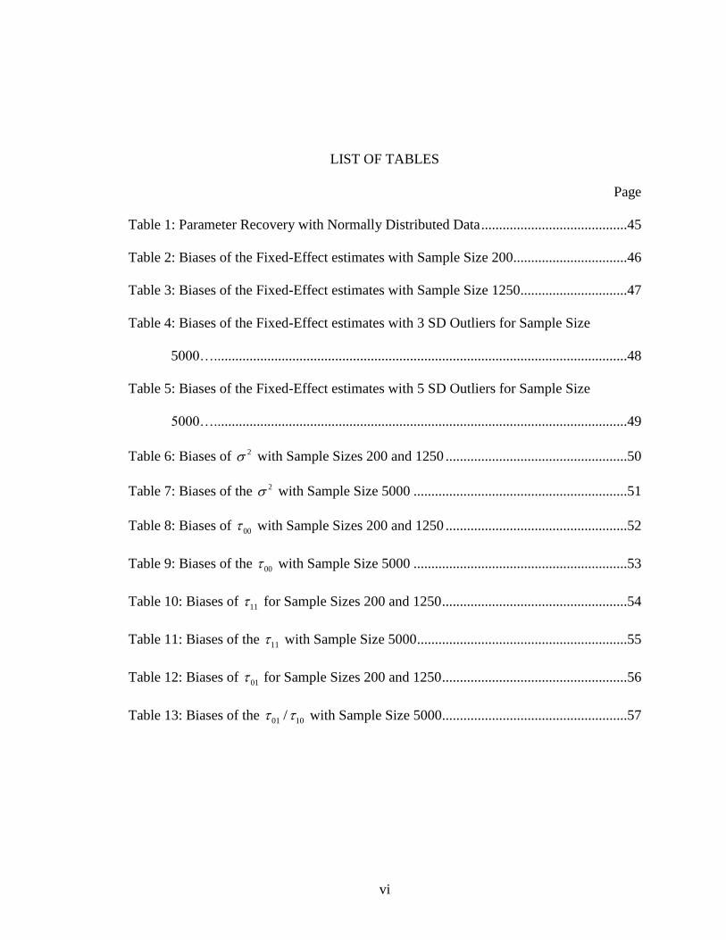
LIST OF TABLES

Page

Table 1: Parameter Recovery with Normally Distributed Data .........................................45

Table 2: Biases of the Fixed-Effect estimates with Sample Size 200 ................................46

Table 3: Biases of the Fixed-Effect estimates with Sample Size 1250 ..............................47

Table 4: Biases of the Fixed-Effect estimates with 3 SD Outliers for Sample Size

5000…....................................................................................................................48

Table 5: Biases of the Fixed-Effect estimates with 5 SD Outliers for Sample Size

5000…....................................................................................................................49

Table 6: Biases of 2 with Sample Sizes 200 and 1250 ...................................................50

Table 7: Biases of the 2 with Sample Size 5000 ............................................................51

Table 8: Biases of 00 with Sample Sizes 200 and 1250 ...................................................52

Table 9: Biases of the 00 with Sample Size 5000 ............................................................53

Table 10: Biases of 11 for Sample Sizes 200 and 1250 ....................................................54

Table 11: Biases of the 11 with Sample Size 5000 ...........................................................55

Table 12: Biases of 01 for Sample Sizes 200 and 1250 ....................................................56

Table 13: Biases of the 01 10/ with Sample Size 5000 ....................................................57

vii

LIST OF FIGURES

Page

Figure 1: The Q-Q Plots and Histograms for the Scaled Residuals with 1 replication of

Normally Distributed Data .....................................................................................58

Figure 2: Q-Q Plots for the Scaled Residuals with 1 Replication on Sample Size 200 .....59

Figure 3: Q-Q plots for the Scaled Residuals with 1 Replication on Sample Size 1250. ..60

Figure 4: Q-Q plots for the Scaled Residuals with 1 Replication on Sample Size 1250 ...61

Figure 5: Q-Q plots for the Scaled Residuals with 1 Replication of 5 SD on Sample Size

5000…....................................................................................................................62

Figure 6: Means of the Dependent Variable of Sample Size 200 ......................................63

Figure 7: Means of the Dependent Variable of Sample Size 1250 ....................................64

Figure 8: Means of the Dependent Variable of Sample Size 5000 ....................................65

Figure 9: Absolute Bias of the Estimate of 00 of Sample Size 200 ..................................66

Figure 10: Absolute Bias of the Estimate of 00 of Sample Size 1250 ..............................67


Figure 12: Absolute Bias of the Estimate of 10 of Sample Size 200 ................................69



Figure 15: Absolute Bias of the Estimate of 2 of Sample Size 200 ...............................72

Figure 16: Absolute Bias of the Estimate of 2 of Sample Size 1250 .............................73

viii


Figure 18: Absolute Bias of the Estimate of 00 of Sample Size 200 ...............................75









Figure 27: Compare the FMLE and Huber-Sandwich Estimator on Standard Errors

Estimation….. ........................................................................................................84

1

CHAPTER 1

INTRODUCTION

Investigating whether the estimation of a model can be easily influenced by

extreme observations or not is of great importance. Based on previous studies, statistical

models with an assumption of normality can be highly sensitive to outlying cases

(Andrew, 1974; Hogg, 1979; Mosteller, 1977). Hierarchical linear models (HLM) can

estimate variance components with unbalanced or nested data and divide the variability

based on different levels. Residual terms at all levels of the HLM are assumed to be

normally distributed. The outliers for a two-level HLM can be the outlying level-1 units

that are far from the normal expectation given the regression equation for each level-2

unit and also can be the outlying level-2 units with an atypical regression coefficient.

Rachman-Moore and Wolfe (1984) indicated that even one outlier at level-1 can “sour”

these estimates of the level-2 unit aggregates and other level-1 unit contributions,

impacting the estimation of fixed effects. Several studies have been conducted indicating

that point estimates and intervals for fixed effects may be sensitive to outliers at all levels

(Seltzer, 1993; Seltzer, Novak, Choi & Lim, 2002). Seltzer and Choi (2003) also asserted

that results were not excessively influenced by one or two extreme outlying values at

level 1 by reanalyzing the real data with level-1 outliers and finding little change in the

fixed effects. Different estimation methods, computational algorithms, assumptions,

sample sizes, and severity of outliers may impact the results of parameter estimation. The

leading sensitivity analyses for the HLM adopted real data analyses and then compared

2

results across different assumptions (Seltzer, 1993; Seltzer & Choi, 2003; Seltzer, Novak,

Choi, & Lim, 2002) or employed robust methods to fit the real data (Rachman-Moore &

Wolfe, 1984). Few studies detected the influence of outliers in details for a specific

subtype of the HLM by using a simulation study. A well-performed simulation study can

explore the bias of parameter estimates in various conditions from the true parameters.

Practical instructions can be provided for educational researchers in using the HLM when

outliers exist.

Hierarchical linear models (HLM) in educational psychology have earned a good

reputation. The applications of the HLM have been explored in various studies in recent

years. Pahlke (2013) applied the HLM to test single-sex schooling and mathematics and

science achievements, and he concluded that students’ performances were not statistically

significantly different as a function of whether the students attended a single-sex school

or not. This claim did not support the single-sex classrooms or schools perspective

proposed by other researchers. (Gurian, Henley, & Trueman, 2001; James, 2009; Sax,

2005). Skibbe (2012) employed HLM to investigate peer effects on classmates’ self-

regulation skills and children’s early literacy growth. The classroom mean of self-

regulation represented the peer effects. This study explored the relationship between

hierarchical levels to determine if classmates’ self-regulation (classroom-mean self-

regulation after controlling for the specific individual’s self-regulation) can predict

students’ literacy achievement (individual level) after controlling the individual self-

regulation. McCoach (2006) applied a piecewise growth model to evaluate the growth of

children’s reading abilities during the first 2-year of schooling. A 3-level (time – student

– school) HLM can locate the factors (i.e., school-level variables: “percentage of

3

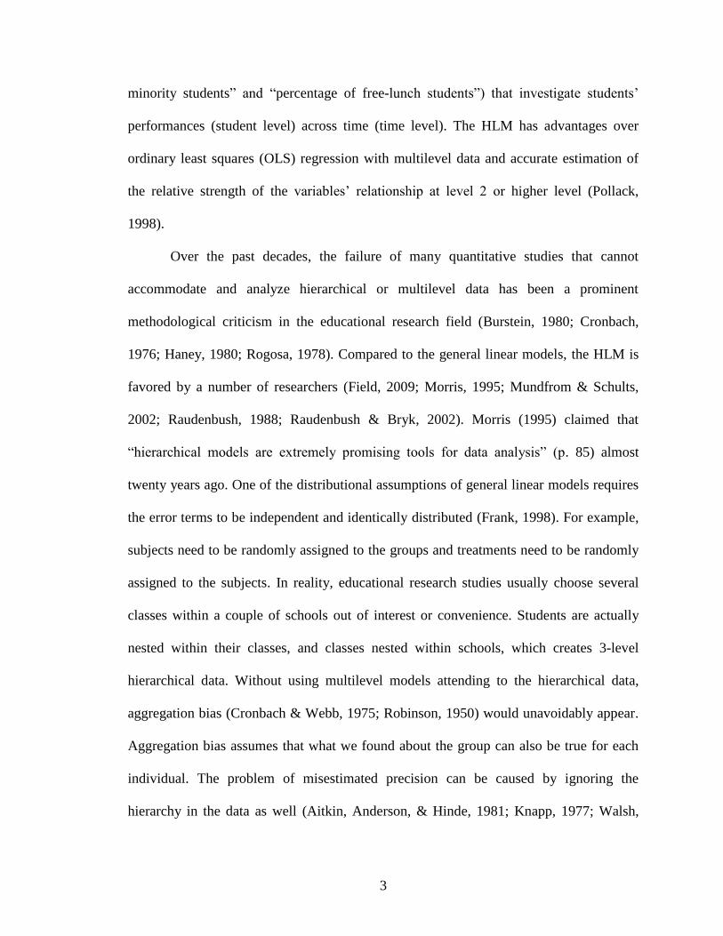
minority students” and “percentage of free-lunch students”) that investigate students’

performances (student level) across time (time level). The HLM has advantages over

ordinary least squares (OLS) regression with multilevel data and accurate estimation of

the relative strength of the variables’ relationship at level 2 or higher level (Pollack,

1998).

Over the past decades, the failure of many quantitative studies that cannot

accommodate and analyze hierarchical or multilevel data has been a prominent

methodological criticism in the educational research field (Burstein, 1980; Cronbach,

1976; Haney, 1980; Rogosa, 1978). Compared to the general linear models, the HLM is

favored by a number of researchers (Field, 2009; Morris, 1995; Mundfrom & Schults,

2002; Raudenbush, 1988; Raudenbush & Bryk, 2002). Morris (1995) claimed that

“hierarchical models are extremely promising tools for data analysis” (p. 85) almost

twenty years ago. One of the distributional assumptions of general linear models requires

the error terms to be independent and identically distributed (Frank, 1998). For example,

subjects need to be randomly assigned to the groups and treatments need to be randomly

assigned to the subjects. In reality, educational research studies usually choose several

classes within a couple of schools out of interest or convenience. Students are actually

nested within their classes, and classes nested within schools, which creates 3-level

hierarchical data. Without using multilevel models attending to the hierarchical data,

aggregation bias (Cronbach & Webb, 1975; Robinson, 1950) would unavoidably appear.

Aggregation bias assumes that what we found about the group can also be true for each

individual. The problem of misestimated precision can be caused by ignoring the

hierarchy in the data as well (Aitkin, Anderson, & Hinde, 1981; Knapp, 1977; Walsh,

4

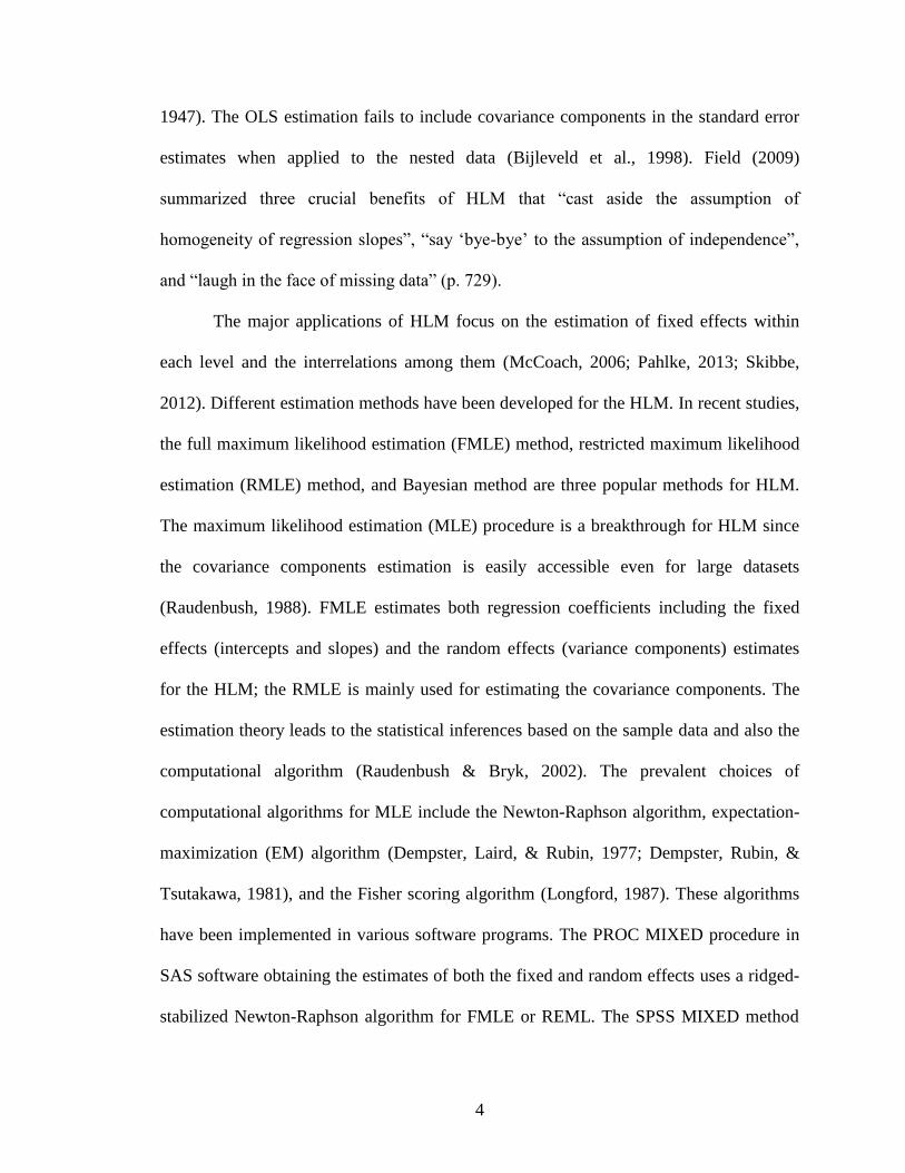
1947). The OLS estimation fails to include covariance components in the standard error

estimates when applied to the nested data (Bijleveld et al., 1998). Field (2009)

summarized three crucial benefits of HLM that “cast aside the assumption of

homogeneity of regression slopes”, “say ‘bye-bye’ to the assumption of independence”,

and “laugh in the face of missing data” (p. 729).

The major applications of HLM focus on the estimation of fixed effects within

each level and the interrelations among them (McCoach, 2006; Pahlke, 2013; Skibbe,

2012). Different estimation methods have been developed for the HLM. In recent studies,

the full maximum likelihood estimation (FMLE) method, restricted maximum likelihood

estimation (RMLE) method, and Bayesian method are three popular methods for HLM.

The maximum likelihood estimation (MLE) procedure is a breakthrough for HLM since

the covariance components estimation is easily accessible even for large datasets

(Raudenbush, 1988). FMLE estimates both regression coefficients including the fixed

effects (intercepts and slopes) and the random effects (variance components) estimates

for the HLM; the RMLE is mainly used for estimating the covariance components. The

estimation theory leads to the statistical inferences based on the sample data and also the

computational algorithm (Raudenbush & Bryk, 2002). The prevalent choices of

computational algorithms for MLE include the Newton-Raphson algorithm, expectation-

maximization (EM) algorithm (Dempster, Laird, & Rubin, 1977; Dempster, Rubin, &

Tsutakawa, 1981), and the Fisher scoring algorithm (Longford, 1987). These algorithms

have been implemented in various software programs. The PROC MIXED procedure in

SAS software obtaining the estimates of both the fixed and random effects uses a ridged-

stabilized Newton-Raphson algorithm for FMLE or REML. The SPSS MIXED method

5

employs a combination of Fisher’s scoring and Newton-Raphson algorithms to obtain the

maximum likelihood estimates. The HLM software implements the EM algorithm and

Fisher’s scoring. The Newton-Raphson algorithm is the default method in the xtmixed

command in Stata. Additionally, the R packages lme() and gls() use a combination of EM

and the Newton-Raphson algorithm (West, Welch, & Galecki, 2007). Snijders and

Bosker (1999) claimed that different computational algorithms would produce the same

estimates, but results may vary regarding the convergence and computational speed.

Lindstorm and Bates (1988) stated that “a well-implemented Newton-Raphson algorithm

is preferable to the EM algorithm or EM algorithm with Aitken's acceleration”. The

FMLE method with the Newton-Raphson algorithm, as a popular method of estimating

the parameters of the HLM, is our interest in this study.

Nonnormality in one of the factors can affect the standard errors for the fixed-

effect estimates, and in turn affects the test statistics in HLM. Applying a robust method

to correct the standard errors is a practical recommendation. An asymptotically consistent

robust method called the “Huber sandwich estimator” is implemented in the SAS

software and the Mplus software, which is popular for correcting standard errors. In the

SAS software, the Huber sandwich estimator can be used in the PROC MIXED and

PROC GLIMMIX procedures to compute the estimated variance-covariance matrix of the

fixed-effects parameters. In the Mplus software, the “MLR” estimator provides the

parameter estimates and robust standard errors which are sandwich or Huber-White

standard errors. Freedman (2006) indicated that the “Huber sandwich estimator” can be

useful when the model is misspecified. He addressed that when the model is nearly

correct, there is no evident benefits from the robustification of the Huber sandwich

6

estimator for correcting the usual standard errors. Additionally, the cost of increasing

robustness requires more computational complexities. If the Huber sandwich estimator

does not perform significantly better than the FMLE method, the cost for the robustness

of the robust method is compromised in dealing with outliers for the HLM.

The purposes of this study are to investigate the biases in the parameters estimates

of the HLM due to outliers, and to check the robustness of the Huber sandwich estimator.

Normality assumptions are assumed at both levels. The FMLE method and Newton-

Raphson computational algorithms are employed for the estimation procedure. The

random-coefficients regression model of the HLM is examined. A simulation study is

performed using the SAS software (Version 9.3) (1) to explore the biases of parameter

estimates with different sample sizes and different numbers of outliers (3 SD and 5 SD),

and furthermore, (2) to examine the sensitivity test for the Huber sandwich estimator in

order to evaluate the performance of this robust method in correcting standard errors and

test statistics of fixed-effect estimates in the presence of outliers.

7

CHAPTER 2

THEORETICAL BACKGROUND

Hierarchical linear model

In educational research, hierarchical data are common. Suppose students’

mathematical abilities over consecutive years, from 6th

grade to 8th

grade, within three

classes of several schools are measured; this data has four levels as mathematic

achievements across years are nested within each student, students are nested within

classes, and classes are nested within schools. Teaching effects or school environments

may create dependency among the data, given that part of the students are in the same

class and part of the classes are in the same school. By using the OLS estimation method

to obtain the parameters of a linear regression model, the hierarchical data violates one

key assumption of OLS estimation that errors are independent from each other. An HLM

is a generalization of traditional linear models. For a 2-level HLM, the regression

functions are computed for each unit at the second level given the first level unit

characteristics and are also regressed across the units at the second level given the second

level unit characteristics. An HLM not only incorporates the hierarchical structure of

data, but also partitions the covariance components and test cross-level effects. Apart

from that, an HLM can be adjusted for non-independence of error terms and also

accommodated to an unbalanced design and missing data.

The HLM share the linearity, normality, and homoscedasticity assumptions with

an OLS regression. However, for an OLS regression, the function should be linear, the

8

total residuals should be normally distributed, and residual variances for all should be

constant. For HLM, linearity should be met at each level, residuals at each level should

be in the univariate or multivariate normal distributions, and the error term at level 1

should be constant. The independence among all the observations that hold by OLS is not

required for HLM. In turn, an HLM has a unique assumption regarding independence that

residuals at different levels need to be uncorrelated and the observations at the highest

level should be independent of each other (Raudenbush & Bryk, 2002).

Raudenbush and Bryk (2002) introduced a general model and six simpler

subtypes of a 2-level HLM, among which the simplest subtype for random intercepts and

slopes is a random-coefficients regression model. We evaluate this model in this study.

The general form of the random coefficients regression model with one random intercept

and one random slope is as follows:

Hierarchical form:

Level-1 0 1ij j j ij ijY X r with 20,ijr N

Level-2 0 00 0j ju with 0 00 01

1 10 11

0,

0

j

j

uN

u

1 10 1j ju

Model in a combined form:

00 10 0 1ij ij j j ij ijY X u u X r , (1)

where i and j represent the level-1 and -2 units, respectively. The ranges for each is

based on the sample size in order to keep the same ratio of numbers of units at two levels.

0 j and 1 j are the random intercept and the random slope of the regression equation

9

correspondingly. ijr represents the error term at level-1 which follows a normal

distribution. 00 and 10 represent the fixed-effect estimates of the random intercept

0 j and the random slope 1 j respectively. In each second level unit, 00 represents the

mean of intercept 0 j and 10 represents the mean of slope

1 j . The random-effect

estimates of the regression coefficients - 0 ju and

1 ju - form a bi-normal distribution. The

variance of 0 ju denotes as 00 , the variance of

1 ju denotes as 11 , the covariance of

0 ju and 1 ju denotes as 01 10/ , and the variance of ijr denotes as 2 . As 01 is equal to

10 , we will only use 01 to represent the covariance of 0 ju and 1 ju in the following

descriptions. For a 2-level regression-coefficients regression model of an HLM, it has

two fixed effects estimates, three random effects estimates, and one error term. The mean

structure part of this regression equation is 00 10 ijX , and the residual part is

0 1j j ij iju u X r .

Maximum likelihood estimation

The MLE produces consistent and efficient estimates. The MLE is also scaled

free and scale invariant. The value of fit functions is the same for the correlation matrix,

covariance matrix, or any other change of scale. The scale invariant refers that the

parameter estimates are not affected by the transformation of variables. Furthermore, the

MLE is the default method of estimation for HLM in most statistical programs (i.e., SAS,

HLM, Mplus, and LISREL).

10

MLE produces parameter estimates of a statistical model that maximize a

likelihood function. The FMLE method is employed in the estimation procedure of this

study. To maximize the likelihood of the data given the hierarchical models, the

probability function is:

,L Y f Y f Y u p u du (2)

where Y is a vector of all level-1 outcomes, u is the vector of all random effects at level

2 or higher levels, is a vector with all the parameters needed to be estimated including

all regression coefficients and covariance components, ,f Y u is the probability

distribution of the outcomes at level 1 given the random effects and parameters, and

p u is the probability distribution of random effects at higher levels given parameters

(Raudenbush & Bryk, 2002).

The fixed-effect estimates in random-coefficients regression model based on

FMLE are as follows:

1

' 1 ' 1ˆm m

j j j j j j

j j

X V X X V y

, (3)

and the variance of is estimated by

' 1 1ˆvar( ) ( )X V X , (4)

where m represents the number of units at level 2. X is the design matrix stacked by

level-2 units, V is the variance-covariance components of the model stacked by level-2

units including the estimates of 00 , 01 , 11 , and 2 (Sullivan, Dukes, & Losina, 1999).

The Newton-Raphson algorithm is one of the numerical analysis methods based on linear

approximation finding the roots of an equation through the iterative process (Ypma,

11

1995). SAS Proc Mixed uses a ridged-stabilized Newton-Raphson algorithm in the log-

likelihood maximization (Sullivan, Dukes, & Losina, 1999).

And the log-likelihood function for the variance-covariance component is as

below (Littell, Milliken, Stroup, & Wolfinger, 1996; Searle, Casella, & McCulloch, &

Schabenberger, O., 2006):

' 11 2, log log 1 log

2 2 2

N NL G R V V

N

, (6)

where represents the residuals of the model, which has the equation of

1 1Y X X V X X V Y . (7)

The estimates of random effects are generated as follows:

1ˆ ˆˆ ˆGX V Y X , (8)

where G is the variance-covariance component matrix, including 00 , 01 , and 11

(Sullivan, Dukes, & Losina, 1999).

The Outliers and Huber Sandwich Estimator

However, the disadvantages of FMLE cannot be ignored. One concern about the

FMLE is the assumption of multivariate normality. The nonnormality affects the

significant tests through the influence of standard errors, even though it does not affect

the parameter estimates (Bollen, 1989). Grubbs (1969) stated that an outlier is one that

seems to deviate markedly from other data of the sample, and it may be merely an

extreme indication of the random variability inherent in the data and it may also be the

result of gross deviation from the experiment process or an error in processing the

numerical data. Barnett and Lewis (Barnett & Lewis, 1994) defined outliers to be the

12

ones are inconsistent with the rest of the data. In educational settings, the extreme values

can be the coding errors or the data entry errors. If it is certain that an outliers is the result

from these errors, the value should be corrected or deleted. However, the outlying

observations may also arise from the random variability of the data which are in the

target population. Researchers would not like to simply delete them. However, the

presence of outliers has serious effects on the modeling, monitoring, and diagnosis of

data (Zou, Tseng, & Wang, 2014). Before applying the model to fit the data with outliers,

it is necessary to do a sensitivity test of the model to the outliers.

As the data become nonnormal, a robust method providing robust standard errors

can be applied. Huber (1967) and White (1982) introduced a robust covariance matrix

estimator, which is commonly used in the generalized estimating equations (GEE,

Diggle, Liang, & Zeger, 1994; Huber, 1967; Liang & Zeger, 1986; White, 1980). The

sandwich estimator is also known as robust covariance matrix estimator (Kauermann &

Carroll, 1999). The Huber sandwich estimator does not change parameter estimates. It

provides the robust standard errors of fixed-effect estimates which in turn corrects the test

of significance (King & Roberts, 2012). Huber sandwich estimator is an implemented

robust method for correcting standard errors in the SAS software and Mplus software. By

using the generalized inverse, it provides a consistent covariance estimation in the

presence of heteroskedasticity (White, 1980).

Different from the usual covariance matrix estimator ' 1 1ˆvar( ) ( )X V X (4), the

Huber sandwich estimator based on the quasi-likelihood GEE computes the covariance

matrix for the fixed-effect estimates as below:

' 1 ' 1 1 ' 1

1

ˆ ˆ( ) ( )( )m

j j j j j j

j

X V X X V V X X V X

, (9)

13

where j refers to the level-2 units and m is the number of units at level 2. ˆ ˆj j jy X ,

is the estimated residual part of the model. jX And jV are the design matrix and the

covariance matrix for unit j, respectively. The general inverse in the equation is

appropriate as the matrix is singular (Liang & Zeger, 1986).

14

CHAPTER 3

A SIMULATION STUDY

Simulation Study Design

A simulation study was performed to investigate the sensitivity of HLM to

outliers. Data sets with three different sample sizes were simulated based on the random-

coefficients regression model. In order to maintain the same ratio of the number of level-

1 units to the number of level-2 units, the three sample sizes set as 200 (20 level-1 units

and 10 level-2 units), 1250 (50 level-1 units and 25 level-2 units), and 5000 (100 level-1

units and 50 level-2 units).

Step 1, normally distributed data were generated based on the random-coefficients

regression model, 00 10 0 1ij ij j j ij ijY X u u X r . The true values of parameters

set as follows: 00 = 5, 01 = 1, 00 = 1, 11 = 4, 01 = 1, and 2 = 4. The correlation

between 00 and 11 was .50. Step 2, two types of outliers (3 SD and 5 SD) were defined

based on the sample standard deviations from the sample means. The mathematical

equation for creating outliers was ˆ*outlierY Y n where n =3 or 5. The sample mean Y

and the sample standard deviation were estimated by using the simulated datasets

without outliers. The 3 SD outliers have three standard deviations from the sample mean.

Similarly, the 5 SD outliers have five standard deviations from the sample mean. All the

outliers were created in the positive direction, in order to avoid the trade-off effects of

outliers. Several specific numbers of outliers with 3 SD and 5 SD are created for the

dependent variable and replaced the same quantity of the simulated data separately.

15

Therefore, the data sets with different sample sizes have different numbers of outliers.

For the datasets with a sample size of 200, 1, 2, 5, 8, 10, and 20 outliers have been

created. The percentage of the outliers in the datasets of sample size 200 are .50%,

1.00%, 2.50%, 4.00%, 5.00%, 10.00%. For the data sets with a sample size of 1250, 2, 5,

10, 25, 50, 75, and 125 outliers have been created. The corresponding percentages are

.16%, .40%, .80%, 2.00%, 4.00%, 6.00%, and 10.00%. For the data sets with a sample

size of 5000, 2, 5, 10, 20, 30, 40, 50, 100, 150, 250, and 500 outliers have been created.

The percentages of those outliers are .04%, .10%, .20%, .40%, .60%, .80%, 1.00%,

2.00%, 3.00%, 5.00%, and 10.00%. With the increases of sample sizes, more options are

available for the number of outliers. For each condition, 100 replications were conducted

to carry out the simulation study. Step 3, the FMLE method with Newton-Raphson

algorithm was adopted to estimate parameters with the correctly specified model that the

random-coefficients regression model. Step 4, the fixed-effect and random-effect

estimates were compared with the true values of the parameters. The indices for the

comparison are absolute bias and relative bias. The bias of a statistic is defined as

ˆ( ) ( )B E , which is the distance of the estimates’ expectation and the estimate.

The absolute bias is the absolute value of the difference between estimates and true

parameters. The relative bias represents the ratio of the absolute bias to the true

parameters, which is the percentage of the relative difference between the expectance of

the estimate and the single estimate. Both the absolute bias and relative bias indicate the

sensitivity of the model with a specific estimation method to the outliers.

The Q-Q plots of the scaled residuals for the dependent variable were used to

display the distribution of residuals. When data are correlated, the vector of residuals

16

instead of each separate residual can be scaled, accounting for the covariances among the

observations. The Cholesky residuals were used in the this study. As described in the

SAS/STAT(R) 9.22 User's Guide, if var( )Y C C , then 1C Y is a vector of uncorrelated

variables with unit variance which has uniform dispersion. Those residuals are expressed

as 1 ˆˆC C Y X .

Step 5, the robust method Huber sandwich estimator was also examined for the

performance of correcting the standard errors and test statistics on the fixed-effect

estimates. The estimated covariance matrix of fixed-effect estimates by the Huber

sandwich estimator was compared with those obtained by the FMLE method.

Simulation Study Results

In order to recover the parameters, the random-coefficients regression model was

employed to fit the simulated data without outliers. The absolute biases and the relative

biases of the estimates were acceptable with all absolute biases less than .20 and relative

biases range from .01% to 8.06% (Table 1). The Pearson correlation between true values

and the estimates was strongly positive, r = .999, p <.01 which provides evidence the

parameters were successfully recovered. The Q-Q plots and histograms for the scaled

residual of the dependent variable indicated that the simulated data were normally

distributed (Figure 1). With sample sizes increasing, the distribution of the data became

more and more normal.

The Q-Q plots of the scaled residuals for the dependent variable showed how the

outliers affect the normal distribution of the data. In the presence of a few outliers, the

distributions of the scaled residuals appeared normal. With larger numbers of outliers,

17

however, the scaled residuals had more variability around the line (Figure 2-5). For the

same numbers of outliers, the model estimations with 5 SD outliers tended to produce

more nonnormal residuals than those with 3 SD outliers. In the presence of extreme

outliers, the scaled residual did not appear to be normally distributed.

The bias of sample means increased with more outliers. For a sample size of 200,

sample mean for data with 10% 3 SD outliers was 1.09 points higher than the sample

mean of the data without outliers. The sample mean of the data with 10% 3 SD outliers

was 1.07 higher than the normal distributed data for a sample size of 1250, and 1.06 for a

sample size of 5000. The sample mean of the data with 10% 5 SD outliers was 1.80

higher than the data without outliers for a sample size of 200, 1.74 for a sample size of

1250, and 1.76 for a sample size of 5000. These results indicated that the sample means

were biased when the data sets had outliers. The sample means of the data with 5 SD

outliers were higher than the data with 3 SD outliers given the same numbers of outliers

and same sample sizes (Figure 6–8); however, the independent t -test indicated no

significant mean difference between different types of outliers, 46 1.45, .16t p .

There is little variation in the sample means across different sample sizes. In addition, the

one-way ANOVA test showed that there were no significant differences in sample means

for different sample sizes, 2,48 1.02, .37F p .

The intercept estimate 00 appeared to be affected evidently by outliers. The

absolute biases of the estimates increased as the number of outliers increased. For a

sample size of 200, the absolute bias displayed increases (Figure 9). The range of relative

biases of 00 for sample size 200 was from .53% to 35.63% (Table 2). From 5% outliers

to 10% outliers, the relative bias of 00 estimate increased by 11.23% with 3 SD outliers

18

and by 18.86% with 5 SD outliers. The largest absolute bias of the estimate 00 was 1.78

and its relative bias was 35.63% when there were 10% 5SD outliers. For a sample size of

1250, the absolute bias increased slowly when the numbers of outliers were less than

.80%; when the numbers of outliers were larger than .80%, the absolute biases increased

rapidly (Figure 10). The range of relative biases of 00 for a sample size of 1250 was

from .81% to 13.75% (Table 3). From 6% outliers to the 10% outliers of a sample size of

200, the relative bias of 00 estimate increased by 7.96% with 3 SD outliers and 13.93%

with 5 SD outliers. For a sample size of 5000, the absolute bias increased slowly when

there were less than 1.00% outliers, but with more than 1.00% outliers, the absolute

biases grew fast (Figure 11). The range of relative biases of 00 given a sample size of

5000 was from .15% to 35.11%. From 5.00% outliers to the 10.00% outliers given a

sample size of 5000, the relative bias in the estimate of 00 increased 10.45% with 3 SD

outliers and 17.97% with 5 SD outliers (Table 4). The one-way ANOVA test for the

differences of absolute/relative biases on 00 across sample sizes was not significant,

2,45 1.19, .31F p . The independent sample t -test for the differences of

absolute/relative biases on 00 between different types of outliers was not significant

either, 46 1.4, .17t p . These results indicate that the relative bias of the intercept

estimate 00 did exist but not significantly varying across sample sizes and types of

outliers.

The slope estimate of 01 with the range of absolute biases less than .15 was much

less susceptible to outliers, compared with the estimate of 00 . The range of relative

19

biases of 01 was from 1.53% to 12.55% for a sample size of 200. The largest absolute

bias of 01 estimate was .14 and its relative bias was 13.75% with 10% of 5 SD outliers

given a sample size of 200 (Table 2). The variation of the absolute biases of 01 for a

sample size of 200 did not have a specific variation pattern (Figure 12). For sample sizes

of 1250 and 5000, the absolute biases with more than 6.00% outliers tended to be high

(Figure 13-14). The other cases still appeared to have random variation with small

absolute biases. The range of relative biases of 01 was from .85% to 13.75% given a

sample size of 1250; and the range of relative biases of 01 was from .84% to 12.56%

given a sample size of 5000. For sample sizes of 1250 and 5000, the largest absolute

biases were .12 and .13 and their relative biases were 11.90% and 12.65% respectively,

given 10.00% of 3 SD outliers (Table 4-5). The absolute biases possessed different

variation patterns with different sample sizes. The one-way ANOVA test for the

differences of absolute/relative biases on 01 across sample sizes was significant,

2,45 4.34, .05F p . Additionally, the independent sample t -test indicated that there

was no significant difference in the absolute bias in the 01 estimation between 3 SD and

5 SD outliers, 77.46 1.23, .22t p . Therefore, the bigger sample sizes would be

helpful for the estimation of 01 .

The outliers have the most influential effects on the estimation of 2 . For a

sample size of 200, with the increase of the numbers of outliers, the absolute biases

increased rapidly (Figure 15). The range of relative biases was from 16.97% to 733.97%,

which are almost 10 to 20 times wider than other estimates. In the presence of 10.00% the

outliers in the data, it had the largest absolute bias as 10.92 and relative bias as 272.89%

20

given 3 SD outliers; and it had the largest absolute bias being 29.36 and relative bias as

733.97% given 5 SD outliers (Table 6). For a sample size of 1250, the absolute biases

increased slowly with the less than .80% outliers; but after this point, the absolute biases

increased evidently (Figure 16). The range of relative biases was narrow down slightly

given a sample size of 1250. The largest absolute biases and relative biases still appeared

with 10.00% outliers. For a sample size of 5000, the absolute biases increased steadily

with less than 1.00% outliers, but increased sharply with more than 1.00% (Figure 17).

The range of relative biases was less wide than it of sample size 1250. The largest

absolute biases and relative biases for 3 SD outliers were 10.22 and 255.52%, and those

for 5 SD outliers were 28.21 and 702.61% respectively, which are obtained with 10.00%

outliers in the data (Table 7). By comparing the results from different sample sizes, it is

concluded that the relative biases can be relatively small when we have larger sample

sizes. The one-way ANOVA test indicated that there was no significant difference

between absolute/relative biases among three sample sizes, 2,45 1.17, .32F p . The

means of the absolute biases for all the estimates with 3 SD and 5 SD outliers were .98

and 2.36. The independent t -test demonstrates that the absolute biases for all the

estimates with 5 SD outliers were significantly higher than those with 3 SD outliers,

119.17 2.17, .05t p . The means of the relative biases for the estimates with 3 SD

and 5 SD outliers were .30 and .66. The relative biases for the estimates with 5 SD

outliers were significantly higher than those with 3 SD outliers as well,

118.72 2.29, .05t p . However, there was no significant difference of

21

absolute/relative biases on 2 across sample sizes, 2,45 1.17, .32F p . Thus, the

distance of outliers has a significant effect on the 2 estimates.

The variance component of the intercept 00 was affected in a similar pattern with

00 . The absolute biases of 00 increased with larger number of outliers (Figure 18-20).

For a sample size of 200, the range of relative biases was from 10.47% to 97.99. The

highest relative bias of 00 with 3 SD outliers was 70.05% when there are 10.00%

outliers. When 10.00% of 5 SD outliers existed in the data sets, the estimate of 00 was

.02 with a highest absolute bias .98 led to a 97.99% relative bias (Table 8). There was an

interaction between numbers and types of outliers in the plot, however, it was not

statistically significant. For a sample size of 1250, the evident increasing linear trend

started from .80% outliers (Figure 19). The range of relative biases was from .78% to

76.97%. When there were 10.00% outliers, the estimates of 00 has the largest absolute

and the relative biases. The absolute biases of 00 with 5 SD outliers appeared to be

higher than those with 3 SD outliers. However, based on the independent sample t -test,

there was no significant difference of absolute biases between 3 SD and 5 SD outliers,

12 .98, .35t p . For a sample size of 5000, the absolute biases seemed to vary

randomly within 1.00%, but increased from the 1.00% point (Figure 20). The range of

relative biases of 00 , given a sample size of 5000, was from .79% to 49.29% (Table 9).

With less than 1.00% outliers, the relative biases were all less than 10.00%. The largest

absolute bias of 00 was .49 and its relative bias was 49.29% when there were 10.00% of

5 SD outliers. The absolute biases of 00 with 5 SD were close to those with 3 SD, and

22

there were no significant differences between them, 20 .47, .64t p . With larger

sample sizes, the minimum and maximum values of relative biases both decreased.

Furthermore, there was an extremely significant difference of absolute/relative biases

across three sample sizes, 2,45 10.56, .001F p .

The effects of variance component of the slope 11 varied with different sample

sizes. For sample size 200, the absolute biases of 11 was high with only .50% outliers;

and then increased slowly before 5.00%; however, the 10.00% outliers can totally

distorted the estimates of 11 (Figure 21). The highest relative bias of 11 with 3 SD

outliers was 30.07% when the percent of outliers is 10.00% (Table 10). When there were

10.00% 5 SD outliers existing in the data sets, the 11 estimate was 3.86 with a standard

error being 2.73. It had the lowest absolute bias .14 leading to a 3.51% relative bias. The

absolute biases of 11 with 5 SD outliers were not significantly different from those with 3

SD outliers based on the independent sample t -test, 10 .43, .68t p . For a sample

size of 1250, there were more variations of absolute biases with less than.80% outliers.

The absolute biases increased from .80% outliers (Figure 22). The range of relative biases

was from .71% to 25.86%. The largest relative bias of 11 was 25.86% with 10.00% 3 SD

outliers. When there were .40% of 5 SD outliers, the estimate 11 had the lowest absolute

bias .03 and relative bias .71% (Table 6). The absolute biases of 11 with 5 SD outliers

were close to those with 3 SD outliers. Based on the independent sample t -test, there was

no significant difference of absolute biases between 3 SD and 5 SD outliers,

12 .10, .93t p . For a sample size of 5000, the absolute biases varied randomly

23

within 1.00%, but increased evidently with more than 1.00% (Figure 23). The range of

relative biases of 11 given a sample size of 5000 was from .97% to 21.95% (Table 11).

With less than 1.00% outliers, the relative biases were all less than 6.00%. The largest

absolute bias of 11 was .88 and its relative bias was 21.95% given 10.00% of 3 SD

outliers. The absolute biases of 11 with 5 SD were close to those with 3 SD as well; and

there was no statistically significant difference between them, 20 .56, .58t p .

Besides, there was an extremely significant difference of absolute biases for all the

estimates of 11 across three sample sizes, 2,45 11.92, .001F p .

The covariance of the intercept 00 and slope 10 was 01 . For a sample size of 200,

the distribution of absolute bias did not display a clear pattern (Figure 24). The absolute

biases appeared to be similar across numbers and types of outliers. The range of relative

biases was from 1.92% to 26.14%. For a sample size of 1250, the range of relative biases

was from 0.18% to 27.05% (Table 12). The absolute biases had evidently changed when

there were more than 4.00% outliers (Figure 25). For a sample size of 5000, the absolute

biases increased fast with more than 1.00% outliers (Figure 26). The range of relative

biases was from 0.35% to 23.56% (Table 13). For the estimates of 01 , there was little

difference between different types of outliers. The independent sample t - test for the

differences of absolute biases on the 01 was not significantly varied between 3 SD and 5

SD outliers, 46 .57, .57t p . In addition, the one-way ANOVA for testing the

differences of absolute biases across sample sizes was significant,

2,45 7.77, .001F p .

24

Comparing FMLE and Huber-sandwich estimator for estimating standard errors

of fixed-effect estimates, there was no significant difference between the FMLE standard

errors and Huber standard errors, according to the independent sample t - tests as follows.

For a sample size of 200, the standard errors of FMLE and of Huber-sandwich estimator

were closer to each other with less than 4.00% of outliers (Figure 27). With more than

4.00% of outliers, the Huber-sandwich estimator provided smaller standard errors than

the FMLE. With 10.00% of outliers, the difference between standard errors of 00 with 5

SD outliers was larger than those with 3 SD outliers. A similar situation happened to

01 as well, but the mean differences between two estimation methods were not

significant given a sample size of 200, 46 .34, .74t p . For a sample size of 1250,

the Huber standard errors of both 00 and 01 with 3 SD outliers were pretty close to the

FMLE standard errors. With 10.00% of 5 SD outliers, the Huber standard error was

slightly smaller than the FMLE standard error of both 00 and 01 estimates given a

sample size of 1250. The mean difference between two estimation methods was also not

significant, 54 .01, .99t p . For a sample size of 5000, it is difficult to distinguish the

distinctions between Huber standard errors and FMLE standard errors for both 00 and

01 estimates with either type of outliers. The mean difference between two estimation

methods was not significant as well, 86 .001, .999t p , which indicated that Huber-

sandwich estimator tended to provide robust standard errors when the outliers were

extreme.

25

CHAPTER 4

DISCUSSION

The outliers had influences on the estimates of random-coefficients regression

model under the FMLE. The estimate of the 2 has been influenced mostly. The outliers

contributed the most to the estimate of 2 . With 10.00% of 5 SD outliers for a sample

size of 200, the relative biases were 733.97%. The effects on the 00 was increasing with

larger numbers of outliers. The biases of 00 with 5 SD outliers were clearly higher than

those with 3 SD outliers. The estimate of 00 , which is the variance of intercept 00 , was

affected in a similar pattern to the estimate of 00 . The estimate of 00 is the mean of

intercept estimate. The estimate of 00 accounts for the variation of the intercept estimate.

With 2 , 00 , and 00 accounting for a large proportion of variation from outliers, the

estimate of 01 has been less influenced when encountered the outliers, as the slope term

of the full model. Besides, the estimate 01 had no specific influence pattern of outliers.

The estimate 11 , which is the variance of 01 , had more random variations before the

numbers of outliers reaching a limit. For example, with a sample size of 200, the biases

of all the numbers, except the case with 10.00% of outliers, seemed to have much

variation. With a sample size of 1250, the approximate linear growth pattern started from

.80% outliers. With a sample size of 5000, the approximate linear trend started from

1.00%. The covariance of the intercept and the slope is 01 , which also displayed much

variation. For a sample size of 200, there was no specific pattern for all the estimates

26

of 01 . With a sample size of 1250, the biases of small percents of outliers (less than

4.00%) decreased but still randomly varied. With a sample size of 5000, the biases within

less than 5.00% outliers were small and had more random variation.

For the estimate of 11 with a sample size of 200, it had the lowest absolute bias,

.14, leading to a 3.51% relative bias given 10.00% of 5 SD outliers, however, the

estimation was not convincing. The standard errors which were estimated with 10.00% of

5SD outliers given a sample size of 200 was very high as well. It, in turn, distorted the

estimate of 11 . The large proportions of the 5 SD outliers on the positive side made the

estimate of 00 being high. The estimates of 01 with sample size 200 had much variation

as well. The 10.00% outliers given a sample size of 200 is a large proportion, which can

no longer be treated as outliers. We would like to call it noise with more than 10.00%

outliers. With 10.00% of 3 SD outliers given a sample size of 200, 1 out of 100

replications of the estimation procedures did not converge with 610 iterations. With

5.00% and 10.00% of 5 SD outliers given a sample size of 200, there are 5 out of 100

replications of the estimation procedures diverged with 610 iterations separately.

Therefore, the stability of parameter estimation of HLM will be compromised with a

large proportion of outliers.

No standard acceptable criterion can be established for the absolute biases and

relative biases. Based on the tables, the researchers can look up the absolute and relative

biases with the corresponding types and numbers of outliers given a specific sample size.

Larger sample size is always good for the estimation. Except the biases of the estimates

00 and 2 , the rest biases of estimates 01 , 00 , 11 , 01 have been significantly different

27

across sample sizes. For sample size 5000, the model estimation produced less biased

parameter estimates with the same number of outliers given a sample size of 1250.

The Huber-sandwich robust estimator corrected the standard errors efficiently

only when there are a large proportion of outliers in the data. Compared to the standard

error estimates with 3 SD outliers, the Huber-sandwich estimator was more efficient in

correcting the standard errors with 5 SD outliers. Therefore, the Huber-sandwich

estimator did not work efficiently in the conditions of this study.

The future studies will investigate the correction for the parameter estimates and

standard errors with robust methods compared with the FMLE. A t -distribution

assumption will be employed in the parameter estimation, compared with the normal

distribution assumption. The influence of level-2 outliers to the HLM will be further

explored. More subtype models of HLM will be included for further examination.

28

CHAPTER 5

CONCLUSION

The simulation study investigates the biases of estimates from true values of the

parameters due to the outliers with three sample sizes, in order to evaluate the sensitivity

of two-level HLM to the outliers under normality assumptions at both levels with FMLE

method and Newton-Raphson computational algorithm. The 2 types of outliers (3SD and

5SD) with specific numbers of outliers vary across different sample sizes have been

created and replaced the same quantity of simulated data. By adding in different types

and numbers of outliers, the model assumption of normality has been violated in various

degrees. Violations of model assumptions have a non-ignorable impact on the model. The

biases of parameter estimates for 2 , 00 , and 00 increased with the larger number of

outliers. For other estimates, the biases have different extents of random variation in

various conditions. The 5 SD outliers have significantly more severe influence than 3 SD

outliers on the estimates of 2 . But for the rest estimates, there is no significant

difference of biases between 3 SD outliers and 5 SD outliers. With a limited number of

outliers, the estimates have very small biases, but the specific limit number varies across

sample sizes. The robust method Huber sandwich estimator corrects the standard errors

efficiently only with a large proportion of outliers.

29

REFERENCE

Aitkin, M., Anderson, D., & Hinde, J. (1981). Statistical modeling of data on teaching

styles. Journal of the Royal Statistical Society, Series A, 144(4), 419-461.

Barnett, V., & Lewis, T. (1994). Outliers in statistical data (Vol. 3): Wiley New York.

Bijleveld, C. C. J. H., van der Kamp, L. J. T., Mooijaart, A., van der Kloot, W. A., van

der Leeden, R., & van der Burg, E. (1998). Longitudinal data analysis: Designs,

models and methods. Thousand Oaks, CA: Sage Publications Ltd.

Bollen, K. A. (1989). Structural equations with latent variables. Oxford England: John

Wiley & Sons.

Burstein, L. J. (1980). The analysis of multi-level data in educational research and

evaluation. Review of Research in Education, 8, 158-233.

Cronbach, L. J. (1976). Research on classrooms and schools: Formulation of questions,

design and analysis.

Cronbach, L. J., & Webb, N. (1975). Between and within-classe ffects in a reported

aptitude-by-treatmenitn teraction: R eanalysis of a study by g. L. Anderson.

Journal of Educational Psychology, 6, 717-724.

Dempster, A. P., Laird, N. M., & Rubin, D. B. (1977). Maximum likelihood from

incomplete data via the em algorithm. Journal of the Royal statistical Society,

39(1), 1-38.

30

Dempster, A. P., Rubin, D. B., & Tsutakawa, R. D. (1981). Estimation in covariance

components models. Journal of the American Statistical Association, 76, 341-353.

Diggle, P., Liang, K.-Y., & Zeger, S. (1994). Analysis of longitudinal data. Oxford:

Clarendon Press.

Field, A. P. (2009). Discovering statistics using spss : (and sex and drugs and rock 'n'

roll) (3rd ed.). Los Angeles ; London: SAGE.

Frank, K. A. (1998). Quantitative methods for studying social context in multilevels and

through interpersonal relations. Review of Research in Education, 171-216.

Freedman, D. A. (2006). On the so-called 'Huber sandwich estimator' and 'robust

standard errors'. The American Statistician(4), 299. doi: 10.2307/27643806

Gurian, M., Henley, P., & Trueman, T. (2001). Boys and girls learn differently : A guide

for teachers and parents. San Francisco: Jossey-Bass.

Haney, W. (1980). Units and levels of analysis in large-scale evaluation. New Directions

for Methodology of Social and Behavioral Sciences, 6, 1-15.

Huber, P. J. (1967). The behavior of maximum likelihood estimates under nonstandard

conditions. Paper presented at the Proceedings of the fifth Berkeley symposium

on mathematical statistics and probability.

IBM Corp. Released 2013. IBM SPSS Statistics for Windows, Version 22.0. Armonk,

NY: IBM Corp.

SAS Institute Inc. (2013). SAS/STAT®13.1 user’s guide. Cary, NC: SAS Institute Inc.

James, A. N. (2009). Teaching the female brain: How girls learn math and science.

Thousand Oaks, CA US: Corwin Press.

31

Kauermann, G., & Carroll, R. J. (1999). The Sandwich Variance Estimator: Efficiency

properties and coverage probability of condence intervals. Available from:

OAIster, EBSCOhost.

King, G., Roberts, M. (2012). How robust standard errors expose methodological

problems they do not fix. Annual meeting of the society for political

methodology, Duke University.

Knapp, T. R. (1977). The unit of analysis problem in applications of simple correlational

research. Journal of Educational Statistics, 2(3), 171-186.

Liang, K.-Y., & Zeger, S. L. (1986). Longitudinal data analysis using generalized linear

models. Biometrika, 73(1), 13-22.

Lindstrom, M. J., & Bates, D. M. (1988). Newton – Raphson and EM algorithms for

linear mixed-effects models for repeated-measures data. Journal of the American

Statistical Association, 83(404), 1014-1022.

Littell, R. C., Milliken, G. A., Stroup, W. W., Wolfinger, R. D. , & Schabenberger, O.

(2006) ‘SAS' System for Mixed Models, 2nd edition, SAS Institute Inc., Cary, NC.

Longford, N. T. (1987). A fast scoring algorithm for maximum likelihood estimation in

unbalanced mixed models with nested effects. Biometrika, 74(4), 817-827.

McCoach, D. B., O'Connell, A. A., Reis, S. M., & Levitt, H. A. (2006). Growing readers:

A hierarchical linear model of children's reading growth during the first 2 years of

school. Journal of Educational Psychology, 98(1), 14-28.

Morris, C. N. (1995). Hierarchical models for educational data: An overview. Journal of

Educational and Behavioral Statistics, 20(2), 190-200.

32

Mundfrom, D. J., & Schults, M. R. (2002). A monte carlo simulation comparing

parameter estimates from multiple linear regression and hierarchical linear

modeling. Multiple Regression Viewpoints, 28, 18-21.

Pahlke, E., Hyde, J. S., & Mertz, J. E. (2013). The effects of single-sex compared with

coeducational schooling on mathematics and science achievement: Data from

korea. Journal of Educational Psychology, 105(2), 444-452.

Pollack, B. N. (1998). Hierarchical linear modeling and the" unit of analysis" problem: A

solution for analyzing responses of intact group members. Group dynamics:

Theory, research, and practice, 2(4), 299.

Rachman-Moore, D., & Wolfe, R. G. (1984). Robust analysis of a nonlinear model for

multilevel educational survey data. Journal of Educational Statistics, 9(4), 277-

293.

Raudenbush, S. W. (1988). Educational applications of hierarchical linear models: A

review. Journal of Educational Statistics, 13(2), 85-116.

Raudenbush, S. W., & Bryk, A. S. (2002). Hierarchical linear models applications and

data analysis methods (second edition). Thousand Oaks, CA, US: Sage

Publications.

Robinson, W. S. (1950). Ecological correlations and the behavior of individuals.

American Sociological Review, 15, 351-357.

Rogosa, D. (1978). Politics, process, and pyramids. Journal of Educational Statistics,

3(1), 79-86.

33

Sax, L. (2005). Why gender matters : What parents and teachers need to know about the

emerging science of sex differences / leonard sax: New York : Doubleday, 2005.

1st ed.

Searle, S. R., Casella, G. and McCulloch, C. E. (1992). Variance Components. Wiley,

New York.

Seltzer, M. (1993). Sensitivity analysis for fixed effects in the hierarchical model: A

gibbs sampling approach. Journal of Educational Statistics, 18(3), 207-235.

Seltzer, M., & Choi, K. (2003). Sensitivity analysis for hierarchical models:

Downweighting and identifying extreme cases using the t distribution Multilevel

modeling: Methodological advances, issues, and applications (pp. 25-52).

Seltzer, M., Novak, J., Choi, K., & Lim, N. (2002). Sensitivity analysis for hierarchical

models employing "t" level-1 assumptions. Journal of Educational and

Behavioral Statistics, 27(2), 181-222.

Skibbe, L. E., Phillips, B. M., Day, S. L., Brophy-Herb, H. E., & Connor, C. M. (2012).

Children's early literacy growth in relation to classmates' self-regulation. Journal

of Educational Psychology, 104(3), 541-553.

Snijders, T. A. B., & Bosker, R. J. (1999). Multilevel analysis: An introduction to basic

and advanced multilevel modeling / Tom A.B. Snijders and roel j. Bosker:

London; Thousand Oaks, Calif. : Sage Publications, 1999.

Sullivan, L. M., Dukes, K. A., Losina, E. (1999). Tutorial in Biostatistics. An

introduction to hierarchical linear modelling. Statistics in medicine.18, 855–888.

Walsh, J. E. (1947). Concerning the effect of the intraclass correlation on certain

significance tests. Annals of Mathematical Statistics, 18, 88-96.

34

West, B. T., Welch, K. B., & Galecki, A. T. (2007). Linear mixed models: A practical

guide using statistical software: CRC Press.

White, H. (1980). A heteroskedasticity-consistent covariance matrix estimator and a

direct test for heteroskedasticity. Econometrica: Journal of the Econometric

Society, 817-838.

White, H. (1982). Maximum likelihood estimation of misspecied models. Econometrica,

50, 1-25.

Ypma, T. J. (1995). Historical development of the Newton-Raphson method. SIAM

review, 37(4), 531-551.

Zou, C., Tseng, S.-T., & Wang, Z. (2014). Outlier detection in general profiles using

penalized regression method. IIE Transactions, 46(2), 106-117.

35

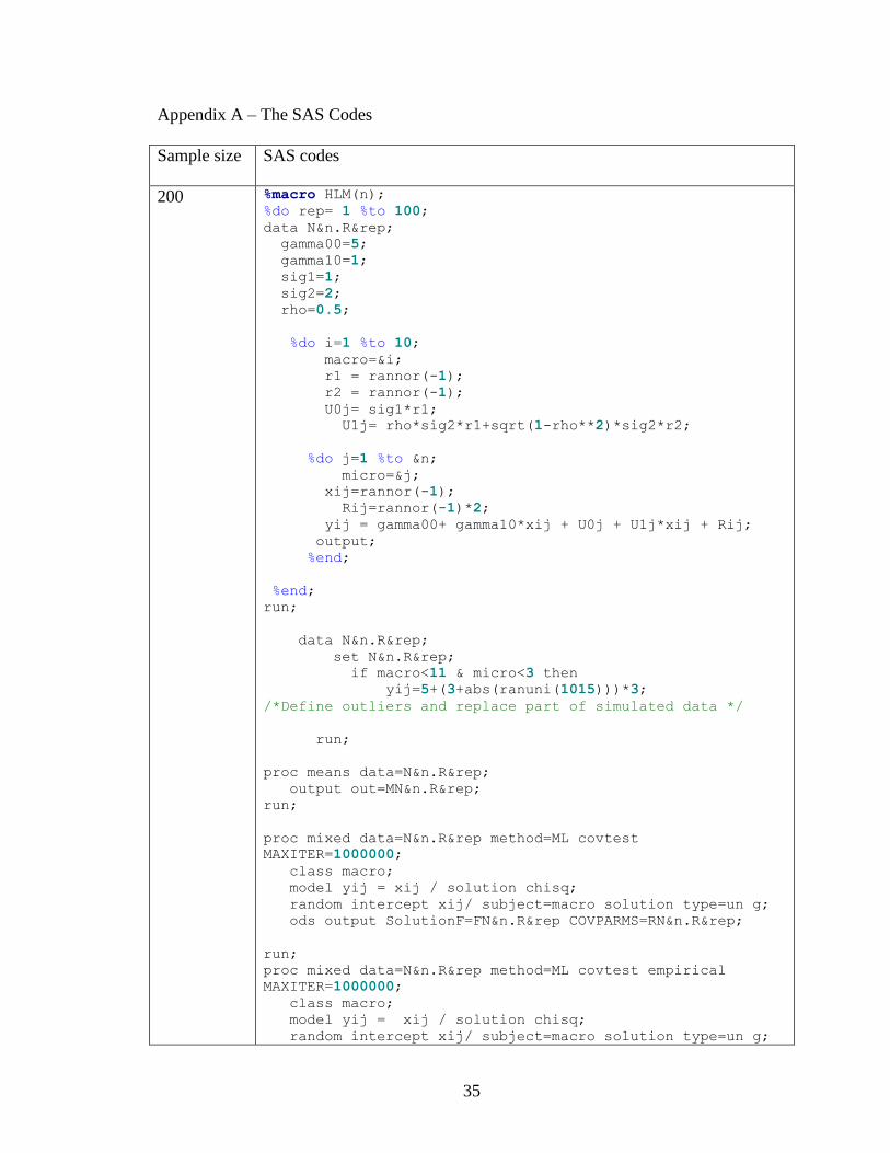
Appendix A – The SAS Codes

Sample size SAS codes

200 %macro HLM(n);

%do rep= 1 %to 100;

data N&n.R&rep;

gamma00=5;

gamma10=1;

sig1=1;

sig2=2;

rho=0.5;

%do i=1 %to 10;

macro=&i;

r1 = rannor(-1);

r2 = rannor(-1);

U0j= sig1*r1;

U1j= rho*sig2*r1+sqrt(1-rho**2)*sig2*r2;

%do j=1 %to &n;

micro=&j;

xij=rannor(-1);

Rij=rannor(-1)*2;

yij = gamma00+ gamma10*xij + U0j + U1j*xij + Rij;

output;

%end;

%end;

run;

data N&n.R&rep;

set N&n.R&rep;

if macro<11 & micro<3 then

yij=5+(3+abs(ranuni(1015)))*3;

/*Define outliers and replace part of simulated data */

run;

proc means data=N&n.R&rep;

output out=MN&n.R&rep;

run;

proc mixed data=N&n.R&rep method=ML covtest

MAXITER=1000000;

class macro;

model yij = xij / solution chisq;

random intercept xij/ subject=macro solution type=un g;

ods output SolutionF=FN&n.R&rep COVPARMS=RN&n.R&rep;

run;

proc mixed data=N&n.R&rep method=ML covtest empirical

MAXITER=1000000;

class macro;



36

ods output SolutionF=EFN&n.R&rep COVPARMS=ERN&n.R&rep;

run;

%end;

%mend HLM;

%HLM(n=20);

data Out5_fixed20;

set Fn20r1 Fn20r2 Fn20r3 Fn20r4 Fn20r5 Fn20r6 Fn20r7 Fn20r8

Fn20r9 Fn20r10 Fn20r11 Fn20r12 Fn20r13 Fn20r14 Fn20r15













Fn20r100;

run;

proc means data=Out5_fixed20 mean;

var Estimate StdErr;

class Effect;

run;

data RobustOut5_fixed20;

set EFn20r1 EFn20r2 EFn20r3 EFn20r4 EFn20r5 EFn20r6 EFn20r7

EFn20r8 EFn20r9 EFn20r10 EFn20r11 EFn20r12 EFn20r13















EFn20r98 EFn20r99 EFn20r100;

run;

proc means data=RobustOut5_fixed20 mean;


class Effect;

run;

data Out5_random20;

set Rn20r1 Rn20r2 Rn20r3 Rn20r4 Rn20r5 Rn20r6 Rn20r7 Rn20r8

Rn20r9 Rn20r10 Rn20r11 Rn20r12 Rn20r13 Rn20r14 Rn20r15

37













Rn20r100;

run;

proc means data=Out5_random20 mean;


class CovParm;

run;

data RobustOut5_random20;

set ERn20r1 ERn20r2 ERn20r3 ERn20r4 ERn20r5 ERn20r6 ERn20r7

ERn20r8 ERn20r9 ERn20r10 ERn20r11 ERn20r12 ERn20r13















ERn20r98 ERn20r99 ERn20r100;

run;

proc means data=RobustOut5_random20 mean;


class CovParm;

run;

data Out5_means20;

set Mn20r1 Mn20r2 Mn20r3 Mn20r4 Mn20r5 Mn20r6 Mn20r7 Mn20r8

Mn20r9 Mn20r10 Mn20r11 Mn20r12 Mn20r13 Mn20r14 Mn20r15










38




Mn20r100;

run;

proc means data=Out5_means20 mean;

var yij;

class _STAT_;

run;

1250 %macro HLM(n);

%do rep= 1 %to 100;

data N&n.R&rep;

gamma00=5;

gamma10=1;

sig1=1;

sig2=2;

rho=0.5;

%do i=1 %to 10;

macro=&i;

r1 = rannor(-1);

r2 = rannor(-1);

U0j= sig1*r1;


%do j=1 %to &n;

micro=&j;

xij=rannor(-1);

Rij=rannor(-1)*2;


output;

%end;

%end;

run;

data N&n.R&rep;

set N&n.R&rep;




run;



run;


MAXITER=1000000;

class macro;




run;

39


MAXITER=1000000;

class macro;




run;

%end;

%mend HLM;%HLM(n=50);

data Out5_fixed50;

set Fn50r1 Fn50r2 Fn50r3 Fn50r4 Fn50r5 Fn50r6 Fn50r7














Fn50r99 Fn50r100;

run;



class Effect;

run;


set EFn50r1 EFn50r2 EFn50r3 EFn50r4 EFn50r5 EFn50r6

EFn50r7 EFn50r8 EFn50r9 EFn50r10 EFn50r11 EFn50r12 EFn50r13















EFn50r98 EFn50r99 EFn50r100;

run;



class Effect;

run;

40

data Out5_random50;

set Rn50r1 Rn50r2 Rn50r3 Rn50r4 Rn50r5 Rn50r6 Rn50r7














Rn50r99 Rn50r100;

run;



class CovParm;

run;


set ERn50r1 ERn50r2 ERn50r3 ERn50r4 ERn50r5 ERn50r6

ERn50r7 ERn50r8 ERn50r9 ERn50r10 ERn50r11 ERn50r12 ERn50r13















ERn50r98 ERn50r99 ERn50r100;

run;



class CovParm;

run;

data Out5_means50;

set Mn50r1 Mn50r2 Mn50r3 Mn50r4 Mn50r5 Mn50r6 Mn50r7







41








Mn50r99 Mn50r100;

run;


var yij;

class _STAT_;

run;

5000 %macro HLM(n);

%do rep= 1 %to 100;

data N&n.R&rep;

gamma00=5;

gamma10=1;

sig1=1;

sig2=2;

rho=0.5;

%do i=1 %to 10;

macro=&i;

r1 = rannor(-1);

r2 = rannor(-1);

U0j= sig1*r1;


%do j=1 %to &n;

micro=&j;

xij=rannor(-1);

Rij=rannor(-1)*2;


output;

%end;

%end;

run;

data N&n.R&rep;

set N&n.R&rep;




run;



run;


MAXITER=1000000;

class macro;


42



run;


MAXITER=1000000;

class macro;




run;

%end;

%mend HLM;%HLM(n=100);

/*n=100;*/

data Out5_fixed100;

set Fn100r1 Fn100r2 Fn100r3 Fn100r4 Fn100r5 Fn100r6


Fn100r14 Fn100r15 Fn100r16 Fn100r17 Fn100r18 Fn100r19














Fn100r98 Fn100r99 Fn100r100;

run;



class Effect;

run;


set EFn100r1 EFn100r2 EFn100r3 EFn100r4 EFn100r5
















43

EFn100r96 EFn100r97 EFn100r98 EFn100r99 EFn100r100;

run;



class Effect;

run;

data Out5_random100;

set Rn100r1 Rn100r2 Rn100r3 Rn100r4 Rn100r5 Rn100r6


Rn100r14 Rn100r15 Rn100r16 Rn100r17 Rn100r18 Rn100r19














Rn100r98 Rn100r99 Rn100r100;

run;



class CovParm;

run;


set ERn100r1 ERn100r2 ERn100r3 ERn100r4 ERn100r5 ERn100r6
















ERn100r97 ERn100r98 ERn100r99 ERn100r100;

run;



class CovParm;

run;

44

data Out5_means100;

set Mn100r1 Mn100r2 Mn100r3 Mn100r4 Mn100r5 Mn100r6


Mn100r14 Mn100r15 Mn100r16 Mn100r17 Mn100r18 Mn100r19














Mn100r98 Mn100r99 Mn100r100;

run;


var yij;

class _STAT_;

run;

45

Table 1

Parameter Recovery with Normally Distributed Data.

Sample

sizes Parameters

True

values Estimates

Standard

errors

Absolute

biases

Relative

biases

200 00 5 5.00 .32 .00 .01%

01 1 1.01 .61 .01 1.11%

2 4 3.96 .42 .04 1.06%

00 1 .93 .51 .07 6.63%

01 10/ 1 .97 .73 .03 3.36%

11 4 3.80 1.80 .20 4.89%

1250 00 5 5.00 .20 .00 .08%

01 1 1.00 .40 .00 .28%

2 4 4.04 .16 .04 .88%

00 1 .98 .30 .02 2.22%

01 10/ 1 .92 .45 .08 8.06%

11 4 3.90 1.13 .10 2.38%

5000 00 5 5.00 .14 .00 .04%

01 1 .97 .28 .03 3.30%

2 4 3.99 .08 .01 .18%

00 1 1.00 .21 .00 .08%

01 10/ 1 .96 .32 .04 3.89%

11 4 3.86 .78 .14 3.40%

Mean .04 2.33%

SD .05 2.40%

Note: The correlation between true values and estimates is r = 0.999 ( p <.01).

46

Table 2

Biases of the Fixed-Effect estimates with Sample Size 200.

Type

of

outliers

Percents Parameters True

values Estimates

Standard

errors

Absolute

biases

Relative

biases

3 SD .50% 00 5 5.03 .32 .03 0.53%

01 1 .93 .60 .07 7.19%

3 SD 1.00% 00 5 5.13 .33 .13 2.56%

01 1 .98 .60 .02 1.99%

3 SD 2.50% 00 5 5.24 .32 .24 4.79%

01 1 .97 .60 .03 3.12%

3 SD 4.00% 00 5 5.44 .32 .44 8.88%

01 1 1.07 .59 .07 7.35%

3 SD 5.00% 00 5 5.53 .32 .53 10.64%

01 1 .95 .60 .05 4.65%

3 SD 10.00% 00 5 6.09 .32 1.09 21.87%

01 1 .93 .58 .07 7.12%

5 SD .50% 00 5 5.10 .33 .10 2.10%

01 1 1.04 .59 .04 4.42%

5 SD 1.00% 00 5 5.19 .33 .19 3.78%

01 1 .98 .58 .02 1.53%

5 SD 2.50% 00 5 5.40 .36 .40 7.99%

01 1 .92 .62 .08 8.01%

5 SD 4.00% 00 5 5.71 .34 .71 14.11%

01 1 1.12 .62 .12 12.49%

5 SD 5.00% 00 5 5.84 .34 .84 16.77%

01 1 .91 .64 .09 9.12%

5 SD 10.00% 00 5 6.78 .41 1.78 35.63%

01 1 .87 .73 .13 12.55%

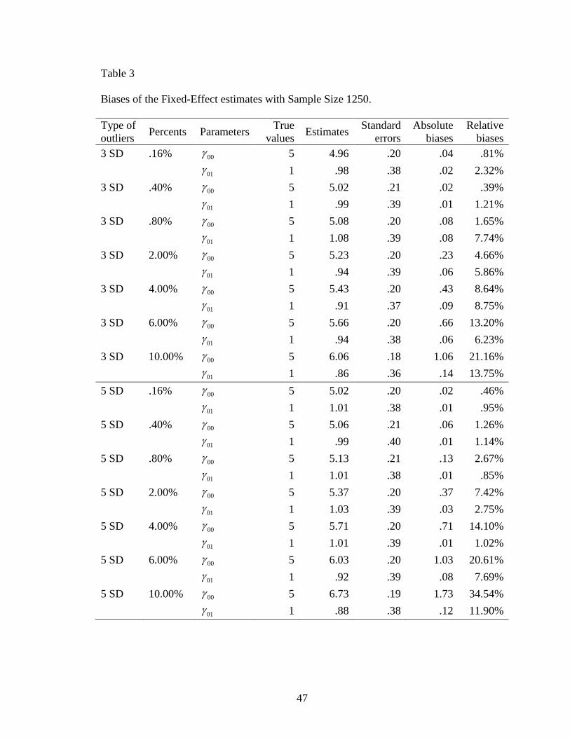
47

Table 3

Biases of the Fixed-Effect estimates with Sample Size 1250.

Type of

outliers Percents Parameters

True

values Estimates

Standard

errors

Absolute

biases

Relative

biases

3 SD .16% 00 5 4.96 .20 .04 .81%

01 1 .98 .38 .02 2.32%

3 SD .40% 00 5 5.02 .21 .02 .39%

01 1 .99 .39 .01 1.21%

3 SD .80% 00 5 5.08 .20 .08 1.65%

01 1 1.08 .39 .08 7.74%

3 SD 2.00% 00 5 5.23 .20 .23 4.66%

01 1 .94 .39 .06 5.86%

3 SD 4.00% 00 5 5.43 .20 .43 8.64%

01 1 .91 .37 .09 8.75%

3 SD 6.00% 00 5 5.66 .20 .66 13.20%

01 1 .94 .38 .06 6.23%

3 SD 10.00% 00 5 6.06 .18 1.06 21.16%

01 1 .86 .36 .14 13.75%

5 SD .16% 00 5 5.02 .20 .02 .46%

01 1 1.01 .38 .01 .95%

5 SD .40% 00 5 5.06 .21 .06 1.26%

01 1 .99 .40 .01 1.14%

5 SD .80% 00 5 5.13 .21 .13 2.67%

01 1 1.01 .38 .01 .85%

5 SD 2.00% 00 5 5.37 .20 .37 7.42%

01 1 1.03 .39 .03 2.75%

5 SD 4.00% 00 5 5.71 .20 .71 14.10%

01 1 1.01 .39 .01 1.02%

5 SD 6.00% 00 5 6.03 .20 1.03 20.61%

01 1 .92 .39 .08 7.69%

5 SD 10.00% 00 5 6.73 .19 1.73 34.54%

01 1 .88 .38 .12 11.90%

48

Table 4

Biases of the Fixed-Effect estimates with 3 SD Outliers for Sample Size 5000.


values Estimates

Standard

errors

Absolute

biases

Relative

biases

.04% 00 5 4.99 .14 .01 .15%

01 1 .99 .28 .01 1.27%

.10% 00 5 5.02 .14 .02 .33%

01 1 .98 .28 .02 2.17%

.20% 00 5 5.03 .14 .03 .56%

01 1 1.01 .28 .01 .84%

.40% 00 5 5.05 .14 .05 1.01%

01 1 .99 .28 .01 1.08%

.60% 00 5 5.07 .14 .07 1.42%

01 1 1.01 .28 .01 1.13%

.80% 00 5 5.08 .14 .08 1.67%

01 1 .98 .28 .02 1.62%

1.00% 00 5 5.11 .14 .11 2.22%

01 1 .98 .28 .02 2.28%

2.00% 00 5 5.22 .14 .22 4.36%

01 1 .98 .27 .02 2.23%

3.00% 00 5 5.34 .14 .34 6.88%

01 1 .99 .27 .01 .89%

5.00% 00 5 5.53 .14 .53 10.57%

01 1 .95 .27 .05 4.74%

10.00% 00 5 6.05 .13 1.05 21.02%

01 1 .87 .25 .13 12.65%

49

Table 5

Biases of the Fixed-Effect estimates with 5 SD Outliers for Sample Size 5000.


values Estimates

Standard

errors

Absolute

biases

Relative

biases

.04% 00 5 4.99 .14 .01 .25%

01 1 .95 .28 .05 5.25%

.10% 00 5 5.02 .14 .02 .48%

01 1 .99 .28 .01 .88%

.20% 00 5 5.04 .14 .04 .88%

01 1 .98 .28 .02 1.62%

.40% 00 5 5.06 .14 .06 1.15%

01 1 .99 .28 .01 1.05%

.60% 00 5 5.11 .14 .11 2.12%

01 1 1.02 .28 .02 2.32%

.80% 00 5 5.14 .14 .14 2.71%

01 1 .97 .28 .03 2.50%

1.00% 00 5 5.18 .14 .18 3.66%

01 1 .99 .28 .01 1.28%

2.00% 00 5 5.34 .14 .34 6.81%

01 1 .98 .28 .02 2.20%

3.00% 00 5 5.50 .14 .50 10.03%

01 1 .96 .28 .04 4.42%

5.00% 00 5 5.86 .14 .86 17.14%

01 1 .97 .27 .03 3.40%

10.00% 00 5 6.76 .13 1.76 35.11%

01 1 .90 .27 .10 9.66%

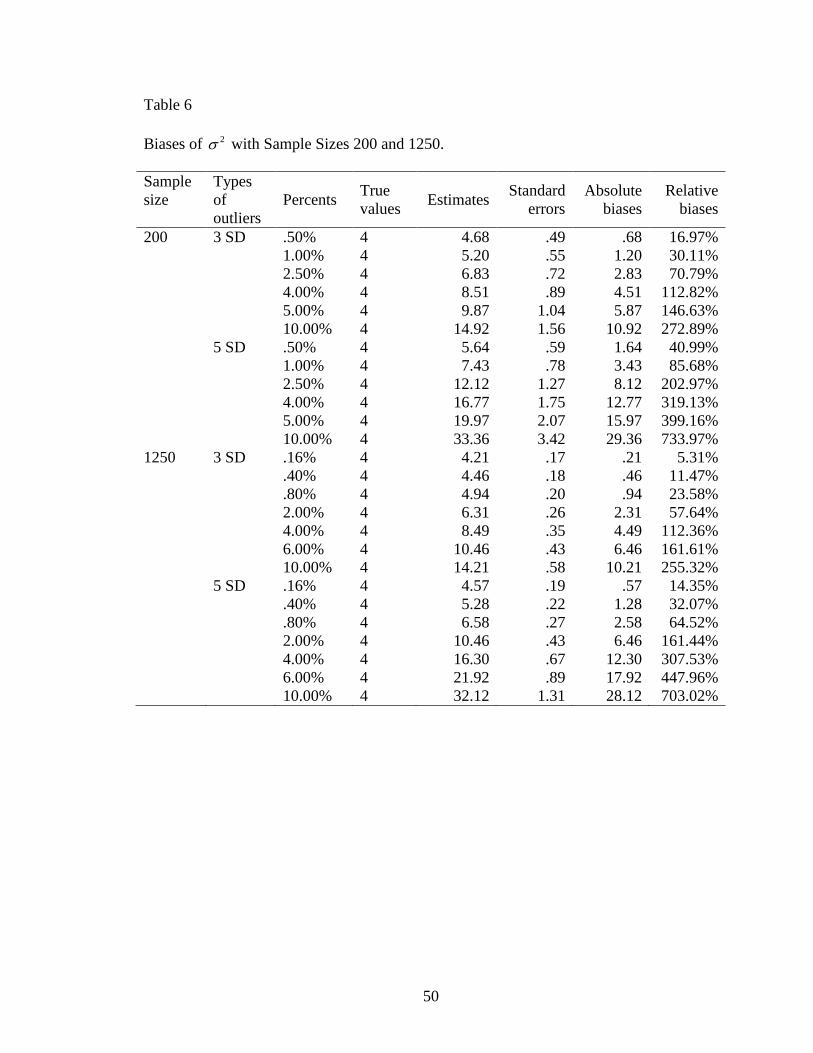
50

Table 6

Biases of 2 with Sample Sizes 200 and 1250.

Sample

size

Types

of

outliers

Percents True

values Estimates

Standard

errors

Absolute

biases

Relative

biases

200 3 SD .50% 4 4.68 .49 .68 16.97%

1.00% 4 5.20 .55 1.20 30.11%

2.50% 4 6.83 .72 2.83 70.79%

4.00% 4 8.51 .89 4.51 112.82%

5.00% 4 9.87 1.04 5.87 146.63%

10.00% 4 14.92 1.56 10.92 272.89%

5 SD .50% 4 5.64 .59 1.64 40.99%

1.00% 4 7.43 .78 3.43 85.68%

2.50% 4 12.12 1.27 8.12 202.97%

4.00% 4 16.77 1.75 12.77 319.13%

5.00% 4 19.97 2.07 15.97 399.16%

10.00% 4 33.36 3.42 29.36 733.97%

1250 3 SD .16% 4 4.21 .17 .21 5.31%

.40% 4 4.46 .18 .46 11.47%

.80% 4 4.94 .20 .94 23.58%

2.00% 4 6.31 .26 2.31 57.64%

4.00% 4 8.49 .35 4.49 112.36%

6.00% 4 10.46 .43 6.46 161.61%

10.00% 4 14.21 .58 10.21 255.32%

5 SD .16% 4 4.57 .19 .57 14.35%

.40% 4 5.28 .22 1.28 32.07%

.80% 4 6.58 .27 2.58 64.52%

2.00% 4 10.46 .43 6.46 161.44%

4.00% 4 16.30 .67 12.30 307.53%

6.00% 4 21.92 .89 17.92 447.96%

10.00% 4 32.12 1.31 28.12 703.02%

51

Table 7

Biases of the 2 with Sample Size 5000.

Type of

outliers Percents

True

values Estimates

Standard

errors

Absolute

biases

Relative

biases

3 SD .04% 4 4.07 .08 .07 1.64%

.10% 4 4.11 .08 .11 2.79%

.20% 4 4.22 .09 .22 5.54%

.40% 4 4.44 .09 .44 10.99%

.60% 4 4.69 .09 .69 17.37%

.80% 4 4.92 .10 .92 23.08%

1.00% 4 5.15 .10 1.15 28.64%

2.00% 4 6.23 .13 2.23 55.63%

3.00% 4 7.29 .15 3.29 82.31%

5.00% 4 9.39 .19 5.39 134.78%

10.00% 4 14.22 .29 10.22 255.52%

5 SD .04% 4 4.13 .08 .13 3.25%

.10% 4 4.31 .09 .31 7.86%

.20% 4 4.63 .09 .63 15.78%

.40% 4 5.25 .11 1.25 31.15%

.60% 4 5.91 .12 1.91 47.83%

.80% 4 6.52 .13 2.52 63.12%

1.00% 4 7.15 .14 3.15 78.68%

2.00% 4 10.11 .20 6.11 152.81%

3.00% 4 13.12 .26 9.12 227.88%

5.00% 4 18.83 .38 14.83 370.71%

10.00% 4 32.10 .65 28.10 702.61%

52

Table 8

Biases of 00 with Sample Sizes 200 and 1250.

Sample

size

Types

of

outliers

Percents True

values Estimates

Standard

errors

Absolute

biases

Relative

biases

200 3 SD .50% 1 .85 .50 .15 14.95%

1.00% 1 .85 .51 .15 14.69%

2.50% 1 .70 .49 .30 29.61%

4.00% 1 .65 .50 .35 35.26%

5.00% 1 .54 .51 .46 46.50%

10.00% 1 .30 .58 .70 70.05%

5 SD .50% 1 .90 .54 .10 10.47%

1.00% 1 .74 .53 .26 26.18%

2.50% 1 .70 .66 .30 29.69%

4.00% 1 .37 .67 .63 63.02%

5.00% 1 .14 .65 .86 85.76%

10.00% 1 .02 .90 .98 97.99%

1250 3 SD .16% 1 .96 .29 .04 4.42%

.40% 1 1.02 .32 .02 2.39%

.80% 1 .95 .30 .05 5.48%

2.00% 1 .88 .29 .12 11.97%

4.00% 1 .82 .28 .18 18.43%

6.00% 1 .76 .28 .24 23.61%

10.00% 1 .56 .24 .44 43.65%

5 SD .16% 1 .92 .29 .08 7.97%

.40% 1 .99 .31 .01 0.78%

.80% 1 .95 .31 .05 5.49%

2.00% 1 .78 .28 .22 22.08%

4.00% 1 .70 .29 .30 30.20%

6.00% 1 .54 .28 .46 46.21%

10.00% 1 .23 .27 .77 76.91%

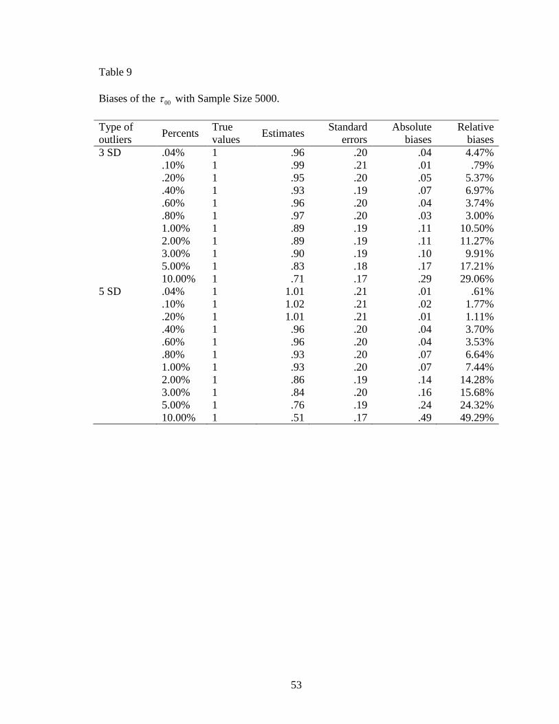
53

Table 9


Type of

outliers Percents

True

values Estimates

Standard

errors

Absolute

biases

Relative

biases

3 SD .04% 1 .96 .20 .04 4.47%

.10% 1 .99 .21 .01 .79%

.20% 1 .95 .20 .05 5.37%

.40% 1 .93 .19 .07 6.97%

.60% 1 .96 .20 .04 3.74%

.80% 1 .97 .20 .03 3.00%

1.00% 1 .89 .19 .11 10.50%

2.00% 1 .89 .19 .11 11.27%

3.00% 1 .90 .19 .10 9.91%

5.00% 1 .83 .18 .17 17.21%

10.00% 1 .71 .17 .29 29.06%

5 SD .04% 1 1.01 .21 .01 .61%

.10% 1 1.02 .21 .02 1.77%

.20% 1 1.01 .21 .01 1.11%

.40% 1 .96 .20 .04 3.70%

.60% 1 .96 .20 .04 3.53%

.80% 1 .93 .20 .07 6.64%

1.00% 1 .93 .20 .07 7.44%

2.00% 1 .86 .19 .14 14.28%

3.00% 1 .84 .20 .16 15.68%

5.00% 1 .76 .19 .24 24.32%

10.00% 1 .51 .17 .49 49.29%

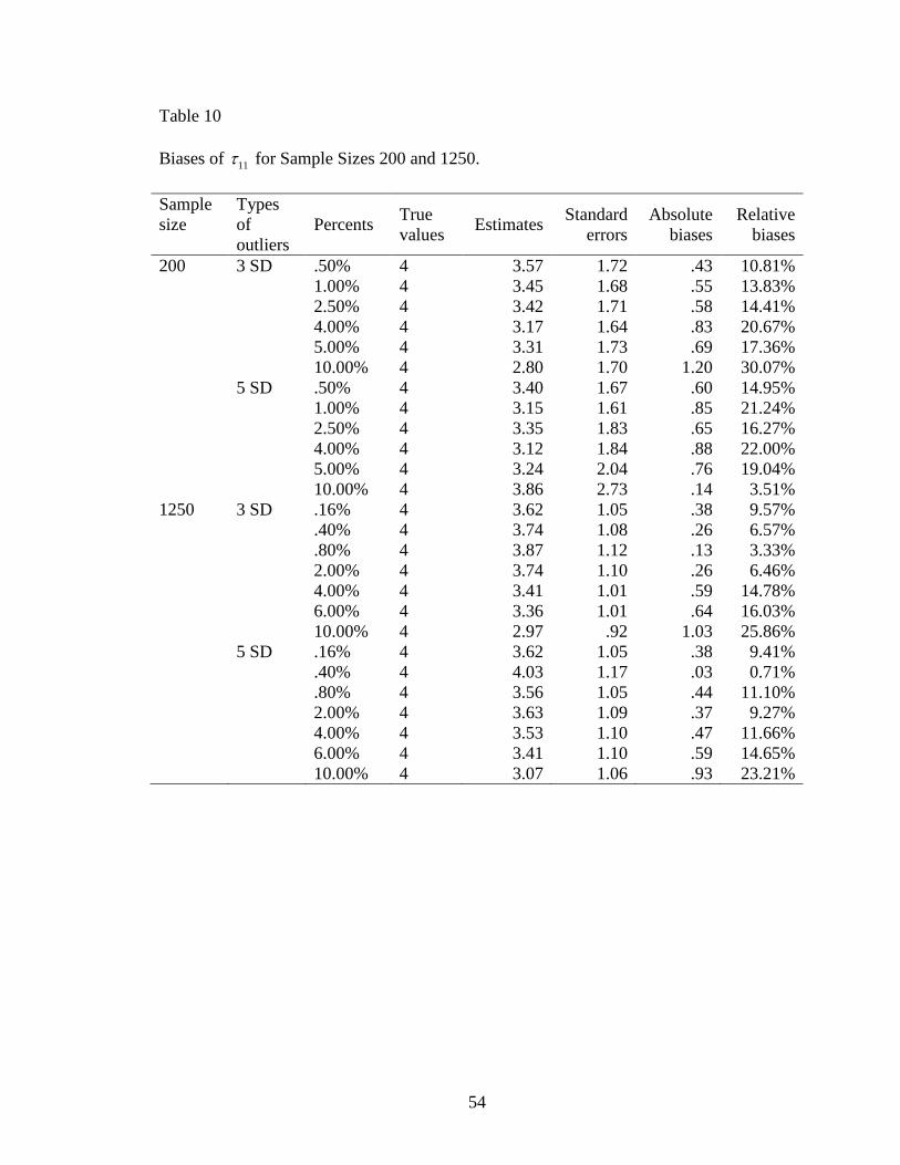
54

Table 10

Biases of 11 for Sample Sizes 200 and 1250.

Sample

size

Types

of

outliers

Percents True

values Estimates

Standard

errors

Absolute

biases

Relative

biases

200 3 SD .50% 4 3.57 1.72 .43 10.81%

1.00% 4 3.45 1.68 .55 13.83%

2.50% 4 3.42 1.71 .58 14.41%

4.00% 4 3.17 1.64 .83 20.67%

5.00% 4 3.31 1.73 .69 17.36%

10.00% 4 2.80 1.70 1.20 30.07%

5 SD .50% 4 3.40 1.67 .60 14.95%

1.00% 4 3.15 1.61 .85 21.24%

2.50% 4 3.35 1.83 .65 16.27%

4.00% 4 3.12 1.84 .88 22.00%

5.00% 4 3.24 2.04 .76 19.04%

10.00% 4 3.86 2.73 .14 3.51%

1250 3 SD .16% 4 3.62 1.05 .38 9.57%

.40% 4 3.74 1.08 .26 6.57%

.80% 4 3.87 1.12 .13 3.33%

2.00% 4 3.74 1.10 .26 6.46%

4.00% 4 3.41 1.01 .59 14.78%

6.00% 4 3.36 1.01 .64 16.03%

10.00% 4 2.97 .92 1.03 25.86%

5 SD .16% 4 3.62 1.05 .38 9.41%

.40% 4 4.03 1.17 .03 0.71%

.80% 4 3.56 1.05 .44 11.10%

2.00% 4 3.63 1.09 .37 9.27%

4.00% 4 3.53 1.10 .47 11.66%

6.00% 4 3.41 1.10 .59 14.65%

10.00% 4 3.07 1.06 .93 23.21%

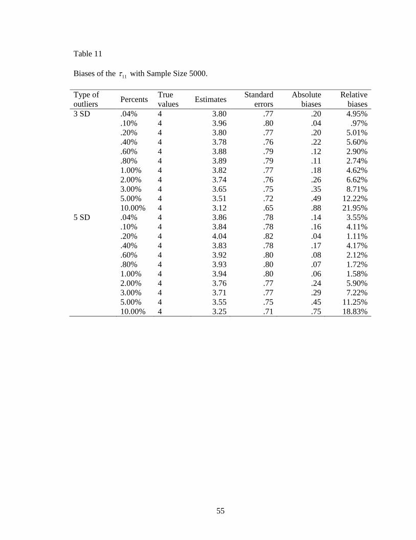
55

Table 11


Type of

outliers Percents

True

values Estimates

Standard

errors

Absolute

biases

Relative

biases

3 SD .04% 4 3.80 .77 .20 4.95%

.10% 4 3.96 .80 .04 .97%

.20% 4 3.80 .77 .20 5.01%

.40% 4 3.78 .76 .22 5.60%

.60% 4 3.88 .79 .12 2.90%

.80% 4 3.89 .79 .11 2.74%

1.00% 4 3.82 .77 .18 4.62%

2.00% 4 3.74 .76 .26 6.62%

3.00% 4 3.65 .75 .35 8.71%

5.00% 4 3.51 .72 .49 12.22%

10.00% 4 3.12 .65 .88 21.95%

5 SD .04% 4 3.86 .78 .14 3.55%

.10% 4 3.84 .78 .16 4.11%

.20% 4 4.04 .82 .04 1.11%

.40% 4 3.83 .78 .17 4.17%

.60% 4 3.92 .80 .08 2.12%

.80% 4 3.93 .80 .07 1.72%

1.00% 4 3.94 .80 .06 1.58%

2.00% 4 3.76 .77 .24 5.90%

3.00% 4 3.71 .77 .29 7.22%

5.00% 4 3.55 .75 .45 11.25%

10.00% 4 3.25 .71 .75 18.83%

56

Table 12

Biases of 01 for Sample Sizes 200 and 1250.

Sample

size

Types

of

outliers

Percents True

values Estimates

Standard

errors

Absolute

biases

Relative

biases

200 3 SD .50% 1 .78 .68 .22 21.98%

1.00% 1 .93 .70 .07 6.69%

2.50% 1 .80 .69 .20 20.49%

4.00% 1 .82 .67 .18 17.89%

5.00% 1 .87 .69 .13 12.78%

10.00% 1 .77 .66 .23 22.70%

5 SD .50% 1 .98 .72 .02 1.92%

1.00% 1 .74 .66 .26 26.14%

2.50% 1 .88 .78 .12 12.02%

4.00% 1 .76 .74 .24 23.87%

5.00% 1 .91 .78 .09 8.51%

10.00% 1 1.25 1.16 .25 24.74%

1250 3 SD .16% 1 .92 .43 .08 7.51%

.40% 1 .94 .45 .06 5.63%

.80% 1 .95 .45 .05 4.99%

2.00% 1 .93 .43 .07 6.77%

4.00% 1 .90 .42 .10 10.20%

6.00% 1 .88 .41 .12 11.59%

10.00% 1 .73 .36 .27 26.64%

5 SD .16% 1 .89 .42 .11 10.53%

.40% 1 1.00 .47 .00 0.18%

.80% 1 .92 .44 .08 8.48%

2.00% 1 .91 .43 .09 8.98%

4.00% 1 .94 .44 .06 6.17%

6.00% 1 .85 .42 .15 14.60%

10.00% 1 .73 .38 .27 27.05%

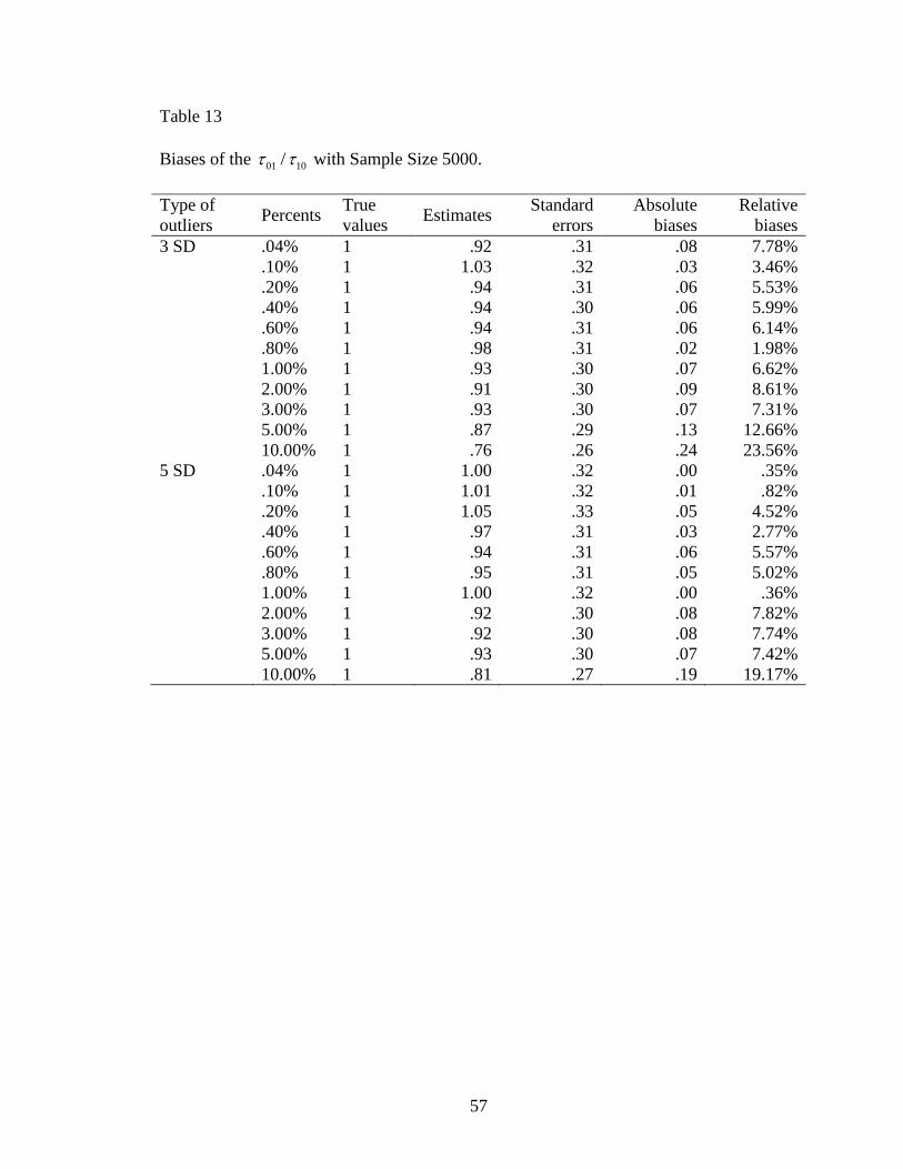
57

Table 13

Biases of the 01 10/ with Sample Size 5000.

Type of

outliers Percents

True

values Estimates

Standard

errors

Absolute

biases

Relative

biases

3 SD .04% 1 .92 .31 .08 7.78%

.10% 1 1.03 .32 .03 3.46%

.20% 1 .94 .31 .06 5.53%

.40% 1 .94 .30 .06 5.99%

.60% 1 .94 .31 .06 6.14%

.80% 1 .98 .31 .02 1.98%

1.00% 1 .93 .30 .07 6.62%

2.00% 1 .91 .30 .09 8.61%

3.00% 1 .93 .30 .07 7.31%

5.00% 1 .87 .29 .13 12.66%

10.00% 1 .76 .26 .24 23.56%

5 SD .04% 1 1.00 .32 .00 .35%

.10% 1 1.01 .32 .01 .82%

.20% 1 1.05 .33 .05 4.52%

.40% 1 .97 .31 .03 2.77%

.60% 1 .94 .31 .06 5.57%

.80% 1 .95 .31 .05 5.02%

1.00% 1 1.00 .32 .00 .36%

2.00% 1 .92 .30 .08 7.82%

3.00% 1 .92 .30 .08 7.74%

5.00% 1 .93 .30 .07 7.42%

10.00% 1 .81 .27 .19 19.17%

58

Sample

sizes Q-Q plots Histograms

200

1250

5000

Figure 1. The Q-Q Plots and Histograms for the Scaled Residuals with 1 Replication of

Normally Distributed Data.

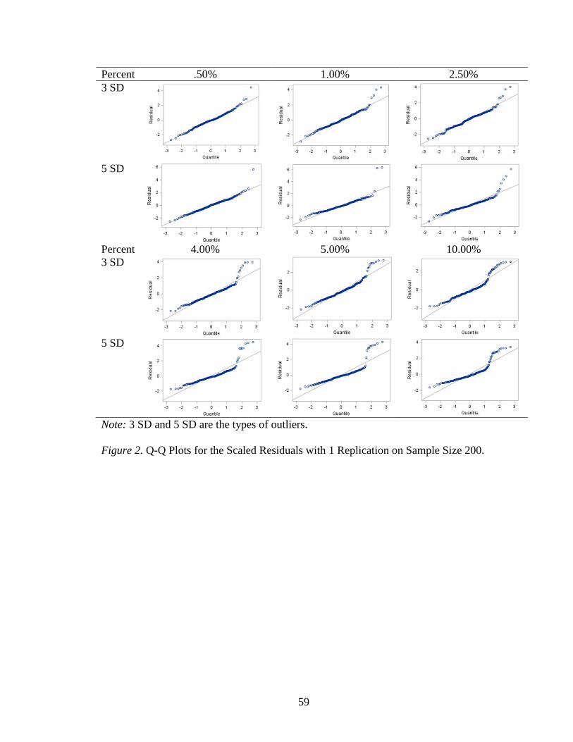
59

Percent .50% 1.00% 2.50%

3 SD

5 SD

Percent 4.00% 5.00% 10.00%

3 SD

5 SD

Note: 3 SD and 5 SD are the types of outliers.

Figure 2. Q-Q Plots for the Scaled Residuals with 1 Replication on Sample Size 200.

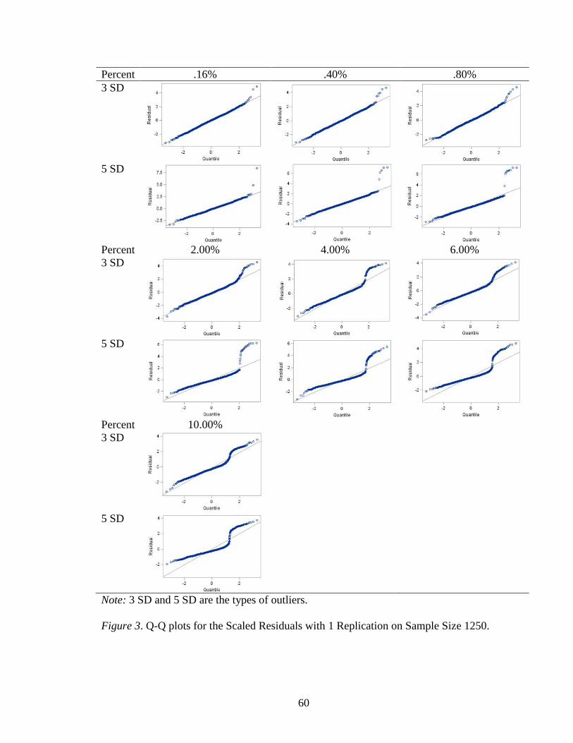
60

Percent .16% .40% .80%

3 SD

5 SD

Percent 2.00% 4.00% 6.00%

3 SD

5 SD

Percent 10.00%

3 SD

5 SD

Note: 3 SD and 5 SD are the types of outliers.

Figure 3. Q-Q plots for the Scaled Residuals with 1 Replication on Sample Size 1250.

61

Percent Q-Q plots Percent Q-Q plots

.04%

1.00%

.10%

2.00%

.20%

3.00%

.40%

5.00%

.60%

10.00%

.80%

Figure 4. Q-Q plots for the Scaled Residuals with 1 Replication of 3 SD on Sample Size

5000.

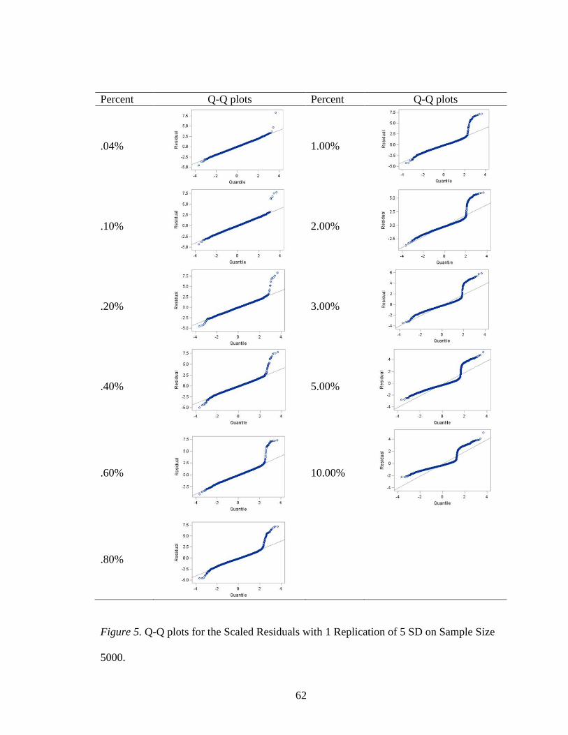
62

Percent Q-Q plots Percent Q-Q plots

.04%

1.00%

.10%

2.00%

.20%

3.00%

.40%

5.00%

.60%

10.00%

.80%

Figure 5. Q-Q plots for the Scaled Residuals with 1 Replication of 5 SD on Sample Size

5000.

63

Figure 6. Means of the Dependent Variable of Sample Size 200.

Percent Of Outliers

64


Percent Of Outliers

65


Percent Of Outliers

66

Figure 9. Absolute Bias of the Estimate of 00 of Sample Size 200.

Percent Of Outliers

67


Percent Of Outliers

68


Percent Of Outliers

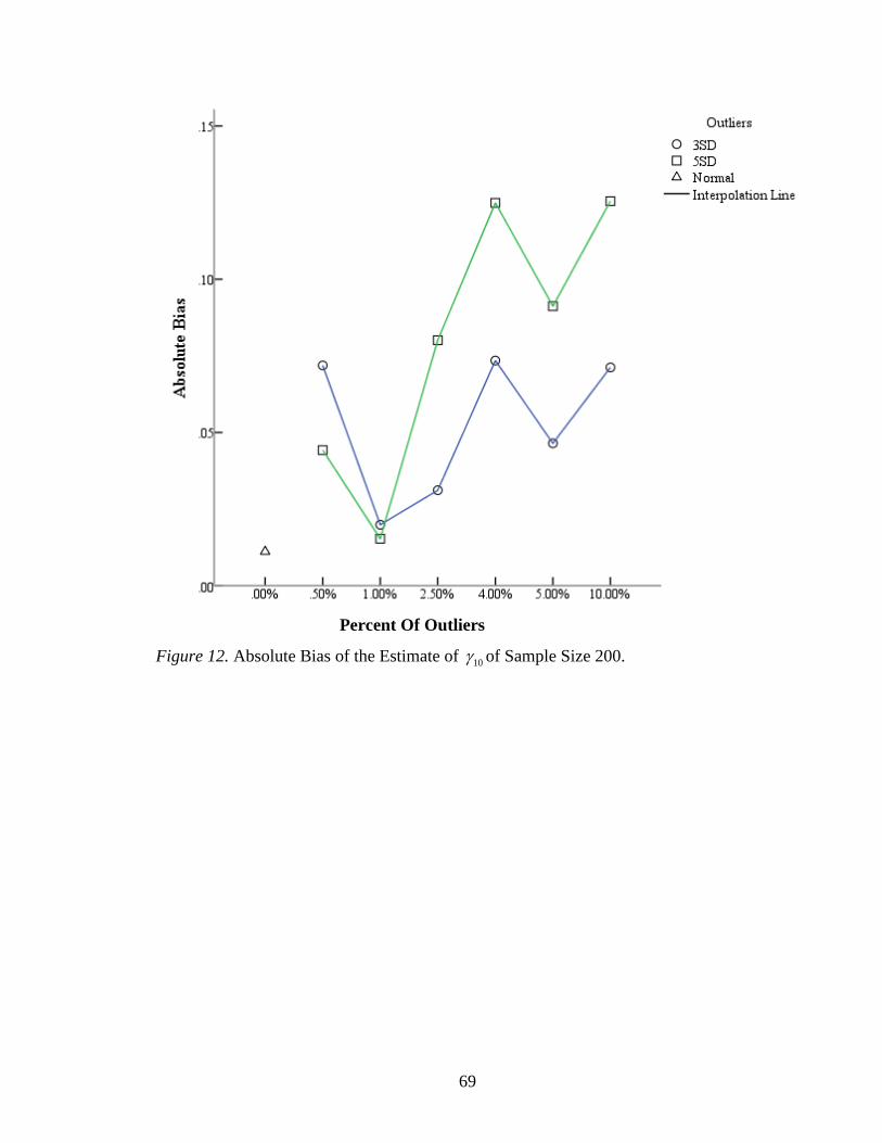
69


Percent Of Outliers

70


Percent Of Outliers

71


Percent Of Outliers

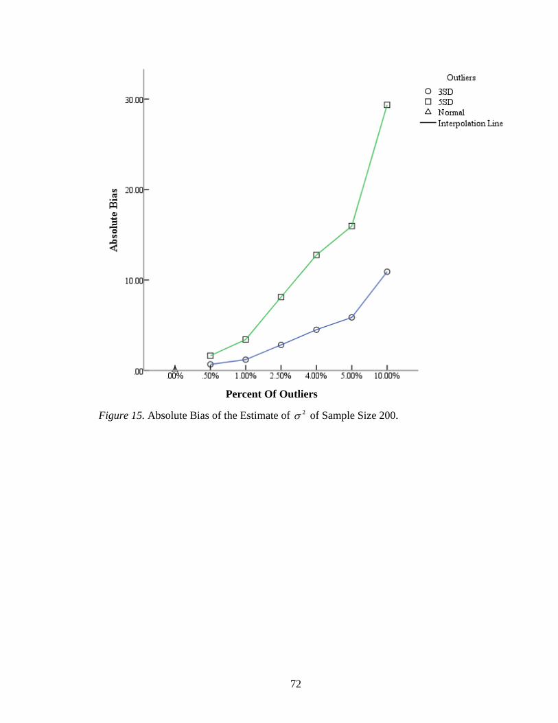
72


Percent Of Outliers

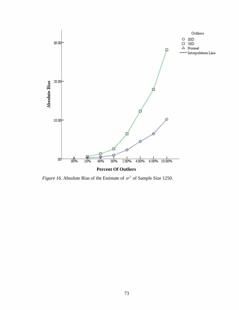
73


Percent Of Outliers

74


Percent Of Outliers

75


Percent Of Outliers

76


Percent Of Outliers

77


Percent Of Outliers

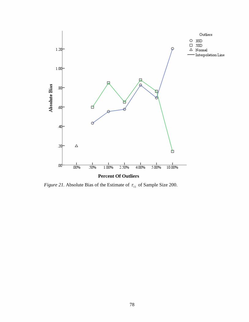
78


Percent Of Outliers

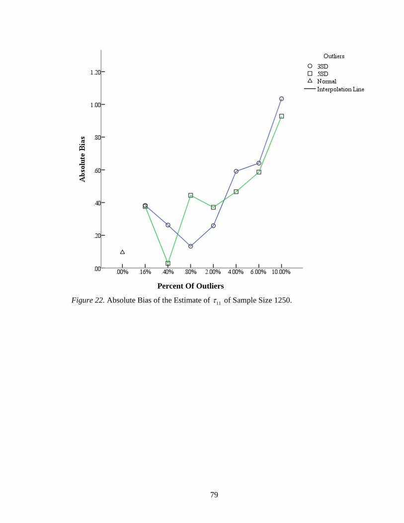
79


Percent Of Outliers

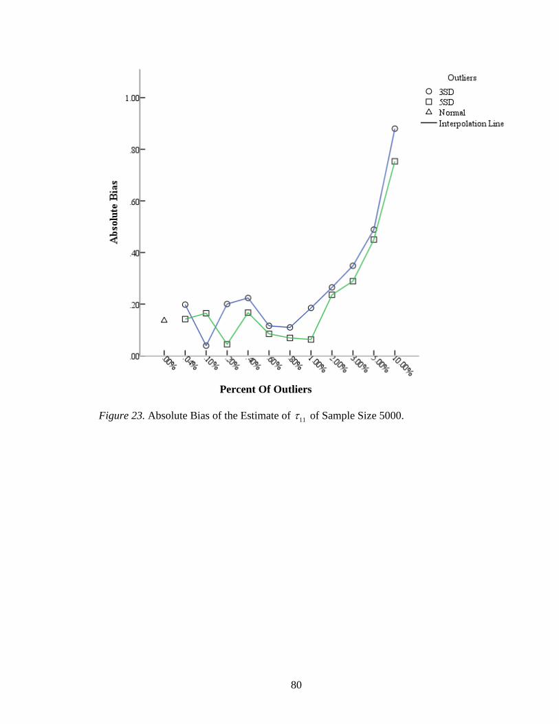
80


Percent Of Outliers

81


Percent Of Outliers

82


Percent Of Outliers

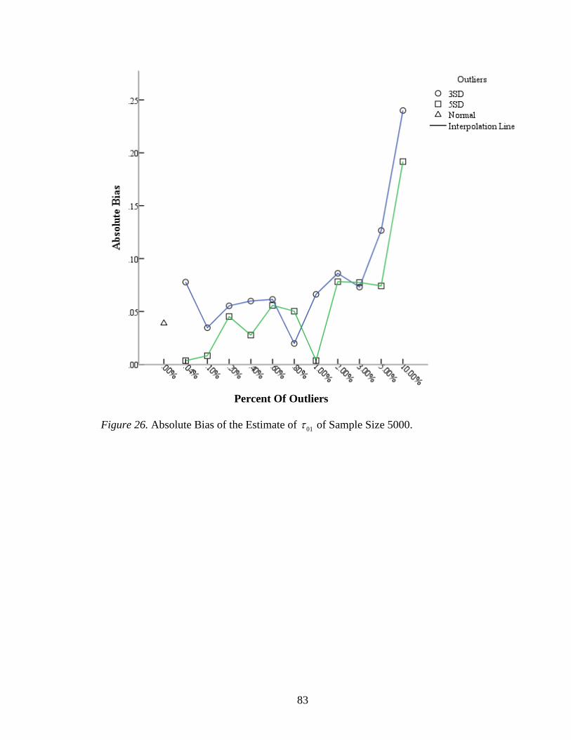
83


Percent Of Outliers

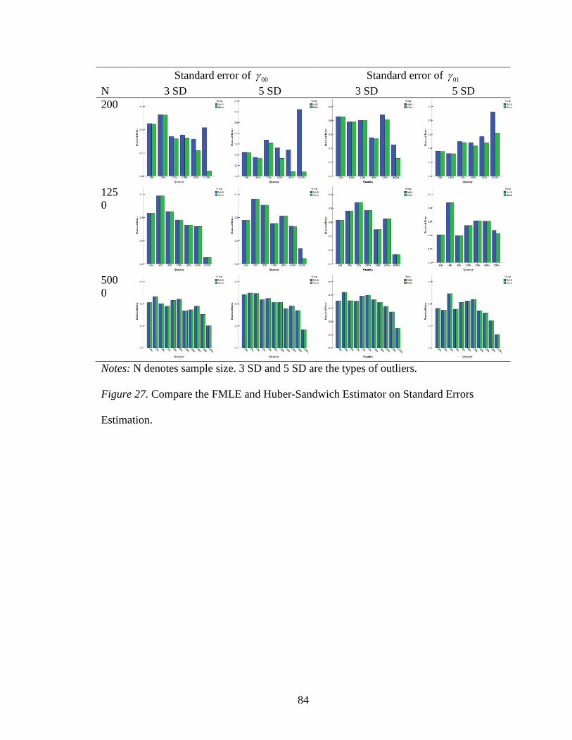
84

Standard error of 00 Standard error of 01

N 3 SD 5 SD 3 SD 5 SD

200

125

0

500

0

Notes: N denotes sample size. 3 SD and 5 SD are the types of outliers.

Figure 27. Compare the FMLE and Huber-Sandwich Estimator on Standard Errors

Estimation.

THE SENSITIVITY OF HIERARCHICAL LINEAR MODELS … · THE SENSITIVITY OF HIERARCHICAL LINEAR MODELS...

Documents

Transcript of THE SENSITIVITY OF HIERARCHICAL LINEAR MODELS … · THE SENSITIVITY OF HIERARCHICAL LINEAR MODELS...