The Sectoral Structure of Poverty During an Adjustment ...

World’ Development, Vol. 19, No. 12, pp. 165S1678, 1991. Printed in Great Britain.

The Sectoral Structure of Poverty During an

0305-750x/91 $3.00 + 0.00 Pergamon Press plc

Adjustment Period: Evidence for Indonesia in the

Mid-1980s

MONIKA HUPPI and MARTIN RAVALLION* The World Bank, Washington, DC

Summary. -During the difficult macroeconomic adjustment period of the mid-1980s, Indonesia was able to maintain the momentum of its progress in reducing aggregate poverty. This paper examines the structure of poverty by sector of employment in Indonesia and how this evolved during 1984-87. A range of poverty measures and decomposition techniques are employed. Gains within the rural sector are found to have been quantitatively important, particularly in Java where there was reasonable growth in both farm and wage incomes associated with crop diversification and continued growth in off-farm employment. Although the aggregate distribution of consumption changed little around its growing mean, substantial intrasectoral shifts in distribution occurred, such that sector growth rates and rates of poverty alleviation were virtually uncorrelated over the period.

1. INTRODUCTION

Indonesia’s economy experienced various external shocks during the mid-1980s, chiefly due to declining prices of the country’s main export good, oil. Public revenues had been heavily dependent on oil exports and were therefore severely affected. The government’s rapid and voluntary adjustment program in response to these shocks included aggregate budgetary con- traction (with planned outlays cut by about one- fifth), rapid and sizable currency devaluations, continuing monetary restraint, and trade, finance, and regulatory reforms (World Bank, 1989). GDP per capita growth rates fell sharply over the period, although remaining (barely) positive. The aggregate sectoral structure of output and employment remained fairly static, slowing the historical decline in agriculture’s share.

In an earlier paper we looked at the evolution of aggregate poverty in Indonesia during 198447 and found that it declined significantly despite the macroeconomic shocks and ensuing adjustments which Indonesia faced during the period (Ravallion and Huppi, 1991). Our qualitative conclusion that poverty decreased proved to be robust with respect to alternative welfare measures, poverty lines, and poverty measures, although the precise quantitative magnitudes of

the poverty measures and their rate of decline are more sensitive to measurement assumptions (Ravallion and Huppi, 1991).

In this paper we examine how the sectoral structure of poverty in Indonesia changed during the adjustment period. There are two possible approaches to such an investigation. One is to use a general equilibrium model to simulate the effects on a base period distribution of explicit external and policy changes. The other is to look at the actual changes in distribution over a period encompassing the changes in external and policy variables. Both have their advantages and dis- advantages; for example, while the former approach gives a clearer resolution of “what caused what,” it typically does so at the cost of many more assumptions. In addition, as we will show later, there are reasons to doubt the

*We are grateful to the Central Bureau of Statistics Indonesia for providing the computer tapes of their household socioeconomic surveys for 1984 and 1987 and to the journal’s referees for their helpful comments on this paper. The paper is a product of a World Bank Research Project, “Policy Analysis and Poverty: Applicable Methods and Case Studies” (RPO 675-04). We are grateful to the World Bank’s Research Com- mittee for their support. These are the views of the authors, however, and should not be attributed to the World Bank.

1653

1654 WORLD DEVELOPMENT

empirical validity of some potentially crucial assumptions of standard simulation approaches in this setting. We follow the second approach in this paper.

The paper has three aims. The first is to describe in detail Indonesia’s profiles of poverty by principal sector of employment, how the profiles changed during 1984-87, and how those changes related to the sectoral pattern of economic growth. Toward this goal, a number of specific empirical questions are addressed: How does the incidence and severity of poverty vary across sectors of employment in Indonesia? Did the pattern of that variation change significantly during the period? What was the relative contribution of poverty alleviation within the various sectors to the reduction in aggregate poverty? How did the pattern of income growth across sectors translate into gains and losses for the poor within those sectors? Were the sectors which grew faster the ones which experienced more rapid poverty alleviation?

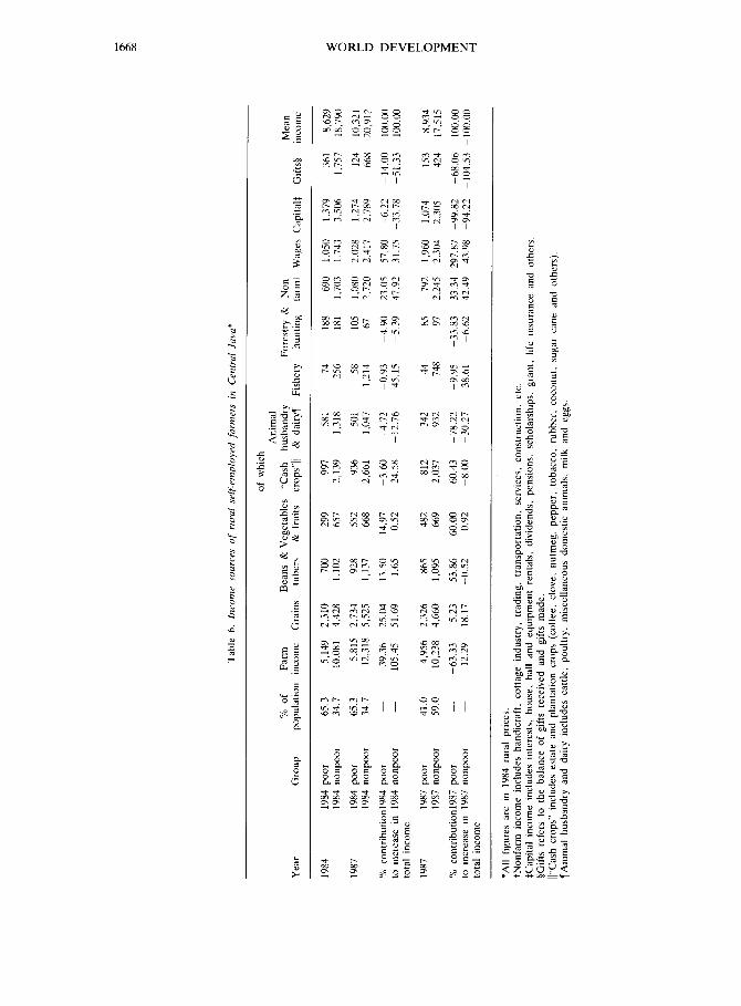
The second aim is to better understand the changes in poverty in the rural farm sector, which we argue is the sector that made the largest contribution to aggregate poverty alleviation. Here we look at both regional dimenions (which are particularly important in Indonesia) and the principal income sources of the rural farm sector. Growth in off-farm income sources has been a significant feature of Indonesian rural development since the 1970s most particularly in Java. There has been, however, some debate as to whether this growth has been as important for the poor as for others.’ We hope to throw light on this issue to assess whether opportunities for income diversification assisted the poor during the period. A related issue concerns the response of incomes of the poor to the changes in relative prices during the mid-1980s. The nominal devaluations shifted farmers’ terms of trade in favor of tradable goods (Ahmed and Chhibber, 1989). To what extent did the poor share in the growth in agricultural export earnings, stimulated by the devaluations? This participation could have occurred either directly, through growth in returns to “cash crops,” or indirectly through growth in wage earnings. Related to the latter possibility, there have been reports of a decline in real agricultural wage rates in Java during this period, although there is conflicting evidence.* The impact on poverty is nonetheless unclear, since it can be argued that it is real wage earnings that we are more concerned about in making income poverty assessments. All these questions call for a detailed analysis of income sources of the poor over the adjustment period.

The paper’s third aim is primarily methodo-

logical, and concerns the empirical validity of assumptions which underlie the first approach mentioned above for studying the effects on the poor of sector-specific economic changes and policy interventions, such as adjustment programs. In “mapping” the final effects of initially sector-specific changes, such as in applied general equilibrium modeling, it is natural (and common) to assume that intrasectoral distributions are static.” Effects on poverty can be simulated by applying predicted sector-specific growth rates to a sector profile of poverty for a base date, assuming distributional neutrality within sectors. Intersectoral changes then propel aggregate distributions and, hence, poverty.

The assumption of neutrality within sectors is convenient for modeling purposes. In addition, and in contrast to our more descriptive approach in this paper, it has the attraction of allowing a deeper understanding of the causal connections between specific adjustment policies and distributional outcomes. Neutrality within sectors, however, may be a questionable assumption in certain circumstances. For example, with relatively flexible labor markets (as is believed to be the case in Indonesia), the mobility of the poor between sectors can result in significant intrasectoral distributional changes, which should not be ignored when considering the impact of sector-specific changes on aggregate poverty. While there is often no practical modeling option to the within-sector neutrality assumption, it is important to know if the assumption is reasonable, and what magnitude of error in simulating aggregate distributional outcomes arises when it fails to hold.

After a discussion of our methodology and data in the following section, the paper examines the question of who were the main beneficiaries of Indonesia’s poverty reduction during 1984-87. Sections 3 and 4 look at average consumption and incomes, and various measures of poverty in different urban and rural sectors of employment. Section 4 also quantifies the contribution of these different sectors to the reduction of aggregate poverty. Section 5 investigates how the sectoral pattern of economic growth affected poverty, and the relevance of intrasectoral distributional changes. Section 6 takes a closer look at the evolution of the principal income sources of rural farm households. Some conclusions are offered in Section 7. An appendix looks at the sensitivity of our main results to some key assumptions made in measuring poverty.

2. DATA AND METHODOLOGY

A measure of poverty has three components:

SECTORAL STRUCTURE OF POVERTY 1655

the measure used to indicate an individual’s living standard, the cutoff point below which an individual is considered to be poor, and the functional form which aggregates the various living standards of the poor into the poverty measure.

The most commonly used indicator of an individual’s living standard is the consumption expenditure of the household in which that individual resides within a certain time frame. It has generally been accepted that consumption expenditure is a better welfare indicator than income. But it is not an ideal measure; for example, it may reveal little of the adverse welfare effect of a decline in the quality of publicly provided social services. In the past, assessments of poverty in Indonesia have been based on consumption expenditure per capita derived from the Central Bureau of Statistic’s (CBS) national socioeconomic survey, referred to as the SUSENAS. We will follow this practice and base our analysis on the data gathered during the two SUSENAS surveys carried out in Febru- ary 1984 and January 1987. These data are available at the household level on computer tapes supplied by CBS. In the appendix we consider the robustness of our results to an alternative welfare indicator based on the share of consumption going to food.

The SUSENAS is a consumption-based survey. It accounts for both market expenditure and consumption from own production and transfers.4 The 1984 and 1987 surveys covered about 50,000 randomly sampled households each and appear to be fully compatible in terms of the methodology used (including sample frame, with some exceptions noted later) and questions asked, and were carried out at about the same time in comparable agricultural years.

All income and expenditure data have been adjusted to February 1984 urban prices, using the Consumer Price Index (CPI). For the purpose of our analysis, the CPI has the shortcoming that it is only constructed for urban areas and doesn’t adequately reflect the consumption pattern of the poor. We have recalculated the index, adjusting for urban-rural price differentials and giving a higher weight to food expenditures, reflecting the typical expenditure pattern of poor households. Specifically, we have increased the food share from 45% to 68%, reflecting the consumption behavior of the bottom 30% of households in 1984, and we have assumed a 10% urban-rural price differential.5 There is no satisfactory regional price index for Indonesia, although differences in regional inflation rates are incorporated in our analysis. We consider the sensitivity of our results to alternative assumptions of regional

price differentials in the appendix. The most worrying aspect of these data is that

the growth rate in real consumption per capita implied by the SUSENAS and CPI is a good deal higher than that implied by the national accounts (Ravallion and Huppi, 1991). We do not know which is closer to the truth. Any overestimation of the rate of growth in mean consumption will lead to an overestimation of the rate of decline in poverty. This problem is less significant in discus- sing the sectoral profiles of poverty and their evolution.6

The choice of a particular poverty line, and hence the cardinal measurement of poverty, is always debatable. Although we have considered a range of poverty lines for this study, we will for brevity’s sake only present results with regard to a monthly per capita expenditure poverty line of Rp. 11,000 (1984 urban prices, Rp. 10,000 in rural prices). In real terms, this point closely approximates the poverty line which has been used in past World Bank studies (Rao, 1984). It is also in close accord with the poverty line one would expect for a country at Indonesia’s mean consumption level, given the empirical relationship between poverty lines and mean consumption across a number of developing and industrialized countries found by Ravallion et ai. (1990). To test the robustness of some of our findings, we make use of stochastic dominance conditions for ordering distributions with respect to a broad class of poverty measures and wide range of poverty lines (Atkinson, 1987; Foster and Shorrocks, 1988). The results are discussed in the appendix.

Various measures of poverty will be considered, aiming to embrace the range of possible value judgments on this issue. We shall consider three members of the Foster, Greer and Thor- becke (FGT) (1984) class of additively decomposable poverty measures P,, each member of which is identified by a nonnegative parameter a. Three FGT measures are used here:’

(a) The headcount index of poverty given by the percentage of the population living in households with average consumptions below the poverty line is used; this is the FGT measure for a = 0. This measure allows us to easily assess variation in the incidence of poverty across sectors. While it is a simple measure to interpret, the headcount index has the disadvantage that it is entirely insensitive to changes below the poverty line; for example, a poor person may become poorer, but measured poverty will not change. Thus the index implicitly treats all of the poor identically; no distinction is made among the 3&40 million poor in Indonesia in terms of the depth or severity of their poverty. It is,


however, plain from at least casual observation that the poor are not all equally poor.

(b) The poverty gap index, defined as the aggregate consumption deficit of the poor as a proportion of the poverty line and normalized by the population size is also used; this is the FGT measure for a = 1. Letting g=(z-y)lz denote the proportionate poverty deficit of a person with income or consumption y below the poverty line z, and setting g=O for the nonpoor, PI is simply the arithmetic mean of g over the whole population. PI allows an assessment of the depth of poverty within sectors.’

(c) Finally, we use the distribution sensitive FGT measure, P2, whereby, instead of weighting the various poverty deficits of the poor equally (as in the previous measure) they are weighted by the deficits themselves. The resulting measure is then simply the mean of the squared proportionate poverty deficits g2. This measure satisfies the main axioms for a desirable poverty measure found in the theoretical literature (for a recent survey see Foster, 1984), including Sen’s (1976) transfer axiom which requires that when income is transferred from a poor person to someone who is poorer, measured poverty decreases. Neither measures (a) nor (b) satisfy this condition. P2 can be interpreted as an indicator of the severity of poverty within sectors.

The FGT measures have the advantage over a number of alternative measures that they are additively separable, such that the aggregate measure is the population weighted mean of the measures for all subgroups of a population. Aside from the obvious computational advantages of that property for constructing decom- positions of poverty (“poverty profiles”), it implies that when any subgroup of the population becomes poorer, aggregate poverty will also increase, ceterisparibus (Foster, Greer and Thor- becke, 1984).

When analyzing the sources of observed reductions in aggregate poverty, we will also make use of a simple decomposition formula which we proposed in Ravallion and Huppi (1991), exploit- ing the additive property of the FGT class of measures. Let P,, denote the FGT poverty measure (or any other additive, population- weighted measure) for sector i with population share ni at date t, where there are m such sectors, and t=1984,1987. Then it is readily verified that:

p,, - p84 = x(pS37 - piX4h84

(Intrasectoral effects)

+ x(ni87 - &X4)PtX4

(Population shift effects)

+ ccpiX7 - pi84)(ntX7 - &X4)

(Interaction effects) (1)

where all summations are over i=l, . ., m. The “intrasectoral effects” tell us the contribution of poverty changes within sectors, controlling for their base period population shares, while the “population shift effects” tell us how much poverty in 1984 was reduced by the various changes in population shares of sectors between then and 1987. The interaction effects arise from the possible correlation between sectoral gains and population shifts.

3. CONSUMPTION AND INCOME BY SECTOR OF EMPLOYMENT

The SUSENAS data tapes provide information on the individual household’s principal source of income. This information is self-reported, with respondents being asked to identify their principal income source from a list of 10 employment sectors, each of which is divided into subgroups of self-employed or hired workers.’ For the purpose of our analysis we will further distinguish between urban and rural areas. Sectors with less than 100 sampled observations have been dropped as results were considered unreliable. Otherwise, results are reported for all sectors identified in the raw data. Our analysis considers 28 sector categories in all. Note that these refer to principal income sources; many households will derive income from more than one sector. In principle, one could further subdivide according to secondary income sources, although one rapidly runs out of degrees of freedom for many sectors. Later we will examine in detail the diversity of income sources for the largest sector, self-employed farmers, for selected regions.

Table 1 provides information about the relative importance of the various sectors in terms of their population shares. It also gives an indication of the relative standard of living within each sector in terms of mean consumption and income in 1984 and 1987. The families of rural self- employed farmers are the largest group, followed by those of rural farm laborers, and then rural traders and urban and rural services. Although the share of people employed by these sectors slightly shifted during 1984-87, their order of importance remained unchanged over these three years. Rural farming (laborers and self- employed) provided the main income for over half of Indonesia’s population in 1984 and for slightly less than half in 1987.

In terms of average per capita consumption, the families of urban financial employees fared best in 1984, followed by those of urban employees in mining, urban employees of the service sector and self-employed urban construc-

Tab

le

1.

Sum

mar

y da

ta o

n se

ctor

s of

em

ploy

men

t*

Inco

met

so

urce

No.

of

sa

mpl

ed

hous

ehol

ds

1984

19

87

Popu

latio

n M

ean

cons

umpt

ion

Gro

wth

M

ean

inco

me

Gro

wth

sh

ares

pe

r ca

pita

ra

te

per

capi

ta

rate

%

R

p./m

onth

t

test

R

p./m

onth

t

test

19

84

1987

19

84

1987

19

84

1987

1.

Farm

ing

L$

U§

R/l

SE

T

U

R

2.

Min

ing

L

u R

SE

R

3.

Indu

stry

L

u R

S

E

U

R

4.

Con

stru

ctio

n L

U

R

S

E

U

R

5.

Tra

de

L

u R

SE

U

R

6.

Tra

nspo

rt

L

U

R

SE

U

R

7.

Fina

nce

L

u

8.

Serv

ices

L

u R

S

E

U

R

396

349

2,99

9 3,

045

976

761

20,7

88

21,4

00

263

181

191

153

232

109

1,07

4 1,

004

671

700

323

307

667

674

876

856

795

864

169

154

131

126

567

549

151

151

2,94

3 2,

927

2,37

9 2,

771

701

588

357

310

460

555

365

411

298

294

3,89

4 4,

282

2,29

7 2,

918

608

635

484

498

0.65

0.

71

18,5

05

15,7

91

-1.8

8 -1

4.67

20

,858

19

,233

-0

.80

-7.7

9 8.

38

7.92

11

,699

13

,606

12

.37

16.3

0 13

,587

15

,547

8.

18

14.4

3 1.

30

1.27

15

,415

18

,619

4.

85

20.7

8 19

,290

23

,467

1.

97

21.6

5 43

.73

39.7

8 13

,444

15

,090

18

.86

12.2

4 16

,034

17

,662

11

.23

10.1

5

0.29

0.

23

0.44

0.

35

0.51

0.

20

2.06

2.

38

1.94

1.

88

0.54

0.

65

1.39

1.

52

1.40

1.

45

2.13

2.

35

0.22

0.

23

0.31

0.

26

0.86

0.

99

0.32

0.

35

4.50

5.

31

6.29

7.

28

1.15

1.

08

0.89

0.

85

0.75

1.

04

1.00

1.

13

0.43

0.

53

5.51

6.

52

4.66

6.

09

0.95

1.

12

1.10

1.

18

32,6

23

32,2

88

-0.1

5 -1

.03

42,0

26

39,6

92

-0.7

4 -5

.55

18,3

87

20,4

24

1.45

11

.08

23.5

81

22,9

32

-0.3

1 -2

.75

12,1

08

14,9

85

3.03

23

.76

17,0

58

19,4

61

0.90

14

.09

23,7

68

25,6

55

2.84

7.

94

27,5

20

28,7

26

1.32

-4

.38

16,0

96

18,8

41

5.15

17

.05

21,1

42

21,7

62

0.30

2.

93

25,4

55

27,3

24

0.99

7.

34

35,7

91

34,4

23

-0.3

7 -3

.82

15,0

59

16,7

40

3.36

11

.16

21,3

31

21,8

53

0.39

2.

45

19,9

05

22,2

25

2.73

11

.66

23,1

38

26,2

27

1.97

13

.35

14,6

57

16,3

55

4.20

11

.58

17,8

27

20,3

00

2.24

13

.87

28,2

25

29,9

87

0.57

6.

24

33,7

63

39,3

21

1.11

16

.46

17,0

48

21,5

14

2.87

26

.20

26,4

66

25,9

94

-0.0

8 -1

.78

27,3

52

31,6

61

3.78

15

.75

30,0

53

35,3

08

3.64

17

.49

17,1

82

19,0

63

1.26

10

.95

21,8

53

21,2

45

-0.2

8 -2

.78

24,6

98

27,9

37

6.66

13

.11

32,1

99

34,5

33

2.13

7.

25

17,2

05

19,3

25

6.28

12

.32

22,8

31

23,8

42

0.95

4.

43

24,0

58

27,0

04

2.63

12

.25

26,5

92

30,6

50

2.68

15

.26

18,2

05

20,7

29

3.02

13

.86

21,8

86

23,8

41

1.76

8.

93

21,1

16

22,7

00

1.28

7.

50

24,2

30

26,6

29

1.27

9.

90

19,6

57

19,9

76

0.21

1.

62

24,7

90

24,5

41

-0.1

2 -1

.00

38,1

93

49,3

07

5.09

29

.10

54,3

11

61,7

01

1.13

13

.61

28,6

90

31,8

46

6.86

11

.00

32,4

20

36,1

34

5.97

11

.46

21,7

20

24,1

34

5.45

11

.11

26,3

12

29,9

75

5.41

13

.92

23,6

91

25,9

22

2.39

9.

42

27,4

44

33,0

82

2.08

20

.54

17,3

73

18,7

18

1.84

7.

74

20,6

23

22,5

45

1.34

9.

32

*Feb

ruar

y 19

84

urba

n pr

ices

. 6.

tr

ansp

orta

tion,

w

areh

ousi

ng

and

com

mun

icat

ion.

tS

ecto

r de

fini

tions

: 7.

fi

nanc

e,

insu

ranc

e,

offi

ce

rent

al,

real

es

tate

an

d of

fice

se

rvic

es.

1.

farm

ing,

hu

sban

dry,

hu

ntin

g an

d fi

shin

g.

8.

com

mun

ity

serv

ices

, so

cial

se

rvic

es

and

pers

onal

se

rvic

es.

2.

min

ing

and

exca

vatin

g.

$L

= la

bore

r/em

ploy

ee.

3.

indu

stri

al

proc

essi

ng.

§U

= ur

ban.

4.

co

nstr

uctio

n.

//R

= ru

ral.

5.

who

lesa

le,

reta

il,

rest

aura

nt

and

hote

l. T

SE

=

self

-em

ploy

ed.


tion workers. This ranking remained the same three years later. Average consumption of all rural employment sectors was significantly below the level of the top three urban sectors in both years. In rural areas, the highest average consumption in 1984 was registered among families of employees in the service sector, followed by people engaged in transportation (self-employed) and employed mine workers. While employees of the service sector continued to rank highest in rural areas in 1987, the second highest average consumption was registered among rural self- employed construction workers, who had ranked much lower in 1984. Rural farm laborers’ households averaged the lowest per capita consumption in both years. The second and third lowest were the families of self-employed rural miners and self-employed rural farmers respectively.

A look at the change in mean consumption of the various employment sectors reveals that average consumption of agricultural workers living in urban areas was the only one to decrease during 1984-87, although this is a small group and the decline is barely significant statistically. Average consumption of rural agricultural workers, on the other hand, increased quite significantly during this period, as did the consumption of rural and urban self-employed farmers. The highest rate of increase in mean consumption occurred among employees of the urban financial sector. Although their average income also increased, it did so to a much lesser extent. Rural self-employed construction workers experienced the second highest proportionate increase in average consumption although, surprisingly, this increase is not re- flected in their mean incomes. In contrast to the relatively large increase in average consumption of rural self-employed construction workers, one finds a comparatively small growth rate of consumption among urban self-employed construction workers. Average consumption and income of rural self-employed miners also grew at impressive rates. The share of people engaged in self-employed rural mining, however, decreased quite significantly, so that the increase in this sector’s average consumption may be due at least partially to emigration of the poorer households. Moreover, the relatively low growth rate of income and consumption in the urban manufacturing sector is also significant.

Although information on average consumption and expenditure can shed some light on differences in typical living standards among various sectors of employment, it does not provide us with any information about the distribution within each sector as relevant to poverty assessments. We turn to this issue in the next section.

4. POVERTY BY SECTOR OF EMPLOYMENT

(a) The poverty profiles

Table 2 contains information about the extent of poverty in the various employment sectors and their relative participation in the alleviation of aggregate poverty during 1984-87. lo

The data in this table clearly illustrate the disparities in poverty incidence, depth, and severity among sectors. In both years, disparities among various urban employment sectors were more pronounced than among rural sectors. In addition, in all cases but one, the poverty measures are higher in rural than in urban areas within a given sector of employment. The highest disparities within one occupational sector were found in mining, where the families of urban mine workers figured among the least poor, and experienced one of the highest relative declines in poverty during 198487, while the families of both self-employed and hired rural miners figured among the poorest groups, although poverty among the latter dropped significantly over the three-year period.

By all measures, and in both years, the highest concentration of poverty was found among farming households, who at the same time make up the largest population proportion. It must, however, be noted that poverty decreased at impressive rates over the period in all farming sectors. In the agricultural sector the highest relative drop in poverty was found among the families of urban self-employed farmers and rural farm laborers, although the latter group retained the highest proportion of poor (53% in 1984 and 38% in 1987). The preferred poverty measure for rural farm laborers, however, shows that the severity of poverty in this group dropped from first to third place over the three-year period. The extent of poverty in this sector was less pronounced than among self-employed rural miners or urban agricultural laborers in 1987. Also noteworthy is that poverty among urban farm laborers dropped, despite a rather significant decrease in the mean value of their consumption.

In 1984, the headcount index of all farming groups (i.e., self-employed and laborers, urban and rural), of self-employed rural miners and of hired rural traders was above the national average. Except for rural traders, the value of the P2 measure of all these groups was also above the national average. With the exception of self- employed rural farmers and rural traders, both poverty measures for the above groups remained above the national average in 1987. In addition,


the headcount index for self-employed rural industrial workers also rose above the national average in 1987. Among the sectors with the lowest incidence of poverty in both years were urban finance, urban services, urban mining, and in 1987, urban transportation. The ranking of these sectors slightly varies by year and poverty measure. In rural areas, services, transportation and industry were among those with the lowest incidence of poverty.

Sectoral poverty as measured by all three poverty measures under consideration dropped significantly in all but one of the sectors of employment during 1984-87. The exception was the urban employees of the financial sector, where all measures showed an increase in poverty, although only the increase in the headcount index was statistically significant. Notwith- standing this poverty increase, the financial sector remained the one with the lowest incidence and extent of poverty.

(b) Sectorulparticipation in aggregatepoverty reduction

Table 2 also provides information on each sector’s relative contribution to aggregate poverty alleviation. These are the “intrasectoral effects” in equation (l), expressed as a percentage of the reduction in aggregate poverty.

The drop in poverty among self-employed rural farmers clearly had the largest influence on aggregate poverty reduction. Over 48% of the reduction in the national headcount index was due to gains in this sector, while it accounted for 55% of the gain in the distribution-sensitive poverty measure. The second most important contribution came from rural agricultural workers, whose reduction in poverty as measured by the headcount index contributed almost 11% to the reduction in the aggregate index, while the decline in this sector’s preferred poverty measure contributed to almost 16% of the aggregate decline. These two groups jointly accounted for 59% of the reduction of the aggregate headcount index and for over 71% of the reduction of the aggregate value of the preferred poverty measure. Note that the rural farm sector’s impressive participation in the reduction of aggregate poverty is due to both significant declines in their poverty measures, and the large share of national poverty accounted for by this sector.

Also noteworthy is the relatively important part of aggregate poverty reduction due to population shifts. Over 13% of the decline in the national headcount index was due to population shifts among various employment sectors, and

over 9% of the decline in the preferred measure can be traced to these shifts. As was seen in Table 1, the sectors which gained in population share were almost all urban, and had initially lower poverty measures. This trend is the main factor underlying the contribution of population shifts to poverty alleviation.

5. POVERTY AND GROWTH ACROSS SECTORS

Both aggregate economic growth and reductions in overall inequalities of consumption contributed to aggregate poverty alleviation in Indonesia during the mid-1980s (Ravallion and Huppi, 1991). Here we look more closely at how the sectoral pattern of Indonesia’s growth affected poverty.

Comparing Tables 1 and 2, there is clearly a strong negative correlation between the poverty indices across sectors and the mean consumptions and incomes of sectors. The simple correlation coefficients between mean consumption and the poverty measures across sectors in 1984 are -.90 for the headcount index, -.83 for the poverty gap index, and - .78 for the distribution sensitive measure. For 1987, the correlation coefficients are -.80, -.73, and -.68 respectively. l1 Similar correlations exist between the poverty measures and mean incomes, although the correlations are not quite as strong (for 1984 they are - .81, - .75, - .71 for the three measures respectively, while for 1987 they are -.76, -.70, and -.65). Figure 1 plots the headcount index in 1984 against the mean income by sector, indicating a sharply decreasing convex relationship. The figure also gives an estimated line of best fit;12 the implied elasticity of the headcount index to mean income is -2.7 at the mean points. It is evident then that the intrasectoral distributions of consumption do not vary much ucross sectors to mitigate the correlation between mean living standards and poverty. The static picture is thus clear.

What is more surprising is that there is little sign of a correlation between the rates of change in the means across sectors and the rates of poverty alleviation. Indeed, the correlations are positive, although small; the simple correlation coefficient between the proportionate change in mean consumption over the period and the proportionate change in poverty is .39 for the headcount index, .37 for the poverty gap index, and .40 for the preferred measure. There is a negligible correlation for the changes in mean income; the coefficients are .13, .14, and .15 respectively. Figure 2 plots the proportionate

Tab

le

2.

Cha

nges

in

pov

erty

by

se

ctor

of

em

ploy

men

t*

Inco

me?

so

urc

e

Hea

dcou

nt

inde

x R

edu

ctio

n

Pov

erty

ga

p in

dex

Red

uct

ion

D

istr

ibu

tion

-sen

siti

ve

Red

uct

ion

!f

du

e to

d

ue

to

u

mea

sure

d

ue

to

sect

oral

se

ctor

al

sect

oral

:

1984

19

87

t te

st*

gain

s 19

84

1987

t

test

ga

ins

1984

19

87

t te

st

gain

s

Nat

ion

al

1. F

arm

ing

L§

Ull

41

.51

34.5

0 -1

.98

0.40

R1

53.0

1 38

.42

-11.

51

10.7

5 S

E**

U

35

.37

20.2

6 -7

.15

1.72

R

43

.91

31.4

2 -2

6.67

48

.04

2.

Min

ing

L

u

5.94

2.

59

-1.7

8 0.

09

R

26.2

9 16

.92

-2.1

3 0.

37

SE

R

48

.29

37.9

1 -1

.82

0.47

3.

Indu

stry

L

u

9.

94

7.01

-2

.40

0.53

R

23

.82

16.2

4 -3

.51

1.30

S

E

U

16.8

0 11

.84

-1.7

8 0.

24

R

35.5

7 23

.38

-4.9

4 1.

49

4.

Con

stru

ctio

n

L

U

18.1

5 13

.70

-2.5

4 0.

55

R

32.6

9 21

.46

-5.1

7 2.

10

SE

U

9.

98

4.70

-1

.84

0.10

R

28

.64

12.4

2 -3

.29

0.44

5.

Tra

de

L

u

8.54

3.

81

-3.3

1 0.

36

R

33.7

9 17

.02

-3.4

1 0.

47

SE

U

9.

97

5.25

-6

.84

1.87

R

26

.75

14.6

3 -

10.7

4 6.

70

%

%

33.0

2 21

.65

-40.

86

%

100.

00

8.52

4.

22

-51.

63

12.2

6 8.

24

-3.3

0 14

.85

7.56

-1

7.58

9.

94

3.95

-8

.90

11.6

9 6.

50

-34.

93

1.44

0.

10

-3.0

5 7.

17

3.28

-2

.83

13.5

7 7.

64

-3.2

4

1.43

0.

97

-2.0

1 5.

42

2.21

-5

.93

3.49

2.

31

-1.6

0 8.

96

3.97

-7

.27

3.45

2.

09

-3.4

5 7.

26

3.70

-5

.97

1.65

0.

96

-1.1

5 7.

09

2.22

-3

.87

1.66

0.

60

-3.1

4 9.

01

4.04

-3

.33

2.10

0.

73

-8.3

8 5.

91

2.34

-

12.2

3

%

100.

00

3.17

0.60

5.

08

14.2

0 5.

79

1.81

4.

06

52.7

8 4.

44

0.09

0.

52

0.40

3.

04

0.71

5.

17

0.22

0.

36

1.45

1.

72

0.15

1.

24

1.62

3.

16

0.44

0.

97

1.76

2.

51

0.04

0.

40

0.35

2.

07

0.21

0.

53

0.37

3.

12

1.43

0.

68

5.22

1.

92

1.24

-4

9.38

2.69

-3

.83

2.17

-1

7.72

1.

20

-8.5

2 1.

99

-34.

09

0.00

-2

.64

0.96

-3

.05

2.67

-2

.80

0.23

-1

.64

0.60

-4

.98

0.65

-1

.85

0.95

-7

.35

0.54

-2

.90

1.05

-5

.25

0.24

-0

.81

0.54

-3

.74

0.14

-2

.81

1.22

-3

.03

0.17

-7

.46

0.58

-

10.9

9

%

i?i

100.

00

z

0.80

15

.71

1.92

55

.52

0.08

0.

48

0.66

0.14

1.

13

0.17

1.

59

0.31

1.

61

0.02

0.

24

0.17

0.

32

1.19

4.

37

6.

Tra

nspo

rt

L

U

11.3

0 2.

72

-6.2

6 R

20

.45

13.6

3 -2

.36

SE

U

26

.27

11.7

0 -5

.91

R

28.9

7 15

.14

-4.6

7

7.

Fina

nce

L

u

8.

Serv

ices

L

u R

S

E

U

R

0.38

2.

37

2.08

5.09

3.

62

-3.2

5 15

.93

9.78

-6

.54

11.8

0 7.

85

-2.3

4 24

.77

20.7

5 -1

.50

Popu

latio

n sh

ifts

In

tera

ctio

n ef

fect

s

0.87

2.

04

0.39

0.

53

4.58

2.

01

0.96

5.

10

2.01

1.

22

6.72

1.

81

-0.0

8 0.

09

0.32

0.71

1.

00

0.56

2.

52

3.37

1.

61

0.33

2.

83

0.87

0.

39

4.85

3.

03

13.2

2 -

- -2

.56

- -

-5.6

6 -3

.62

-5.1

5 -6

.42 1.22

-4.4

4 -7

.38

-4.6

2 -2

.96

-

0.44

0.

55

0.07

0.

53

1.51

0.

47

0.54

1.

54

0.50

1.

14

2.29

0.

36

-0.0

2 0.

02

0.09

0.56

0.

29

0.13

1.

91

1.08

0.

46

0.43

1.

02

0.17

0.

47

1.51

0.

67

10.4

4 -

- -4

.26

- -

-4.6

2 -3

.59

-4.1

5 -5

.79

0.98

-4.5

0 -6

.04

-4.5

3 -3

.56

0.29

0.

48

0.40

1.

00

-0.0

2

0.46

1.

50

0.42

0.

48

9.40

-4

.50

*Com

pone

nts

do

not

add

up

to t

otal

ex

actly

be

caus

e of

mis

sing

da

ta

for

som

e ho

useh

olds

, an

d be

caus

e a

num

ber

of s

ecto

rs

are

omitt

ed

due

to s

mal

l sa

mpl

e si

zes

and

beca

use

of

roun

ding

. tS

ecto

r de

fini

tions

: 1.

fa

rmin

g,

husb

andr

y,

hunt

ing

and

fish

ing.

2.

m

inin

g an

d ex

cava

ting.

3.

in

dust

rial

pr

oces

sing

. 4.

co

nstr

uctio

n.

5.

who

lesa

le,

reta

il,

rest

aura

nt

and

hote

l. 6.

tr

ansp

orta

tion,

w

areh

ousi

ng

and

com

mun

icat

ion.

7.

fi

nanc

e,

insu

ranc

e,

offi

ce

rent

al,

real

es

tate

an

d of

fice

se

rvic

es.

8.

com

mun

ity

serv

ices

, so

cial

se

rvic

es

and

pers

onal

se

rvic

es.

$Sig

nifi

canc

e te

sts

of

the

diff

eren

ces

betw

een

pove

rty

mea

sure

s ar

e ba

sed

on

Kak

wan

i’s

(199

0)

form

ulae

fo

r th

e st

anda

rd

erro

rs

of

Pa.

IL

= la

bore

r/em

ploy

ee.

/IU

=

urba

n.

nR

= ru

ral.

**S

E

= se

lf-e

mpl

oyed

.


60

20 30 40 50 60

Mean income, RpOOO/ps/mn, 1984

Figure 1. Poverty by sector 1984 plotted against mean income

. .

l .

. .’

.

. .

. l m n

. . .

.

.

.

.

. .

-80 1 I I I I I I I

-10 -5 0 5 10 15 20 25

Percentage change in mean income 1984-87

Figure 2. Changes in poverty 1984-87 plotted against change in income.

changes in the headcount index against the income growth rates (over three years). The sectors which experienced the more rapid rates of poverty alleviation were clearly not (as a rule) the sectors which had the highest rates of income growth; nor were the poorly performing sectors in terms of growth the ones which fared worst in terms of their progress in alleviating poverty.

This is not to say that growth did not alleviate poverty over the period. From our aggregate analysis it is clear that growth accounted for the majority of the observed change in poverty; for example, if one assumed that growth was distributionally neutral across the whole economy

over the period then one would underestimate the change in the headcount index by only 14%, although it rises to 33% for the P2 poverty measure, reflecting the fact that it is distribution sensitive (Ravallion and Huppi, 1991). Distribu- tional effects were of secondary importance in the aggregate picture.

What these new calculations suggest is that distributional effects within sectors were much more important to the sectoral pattern of poverty alleviation than were the aggregate distributional effects. There were significant shifts in the distributions of consumption within sectors over the period, mitigating the effects of growth. This


trend could well be explained by the mobility of the poor between employment sectors.

Table 3 gives our estimates of the contribution of distributionally neutral growth to poverty alleviation across sectors. To arrive at these figures, we have first estimated the change in poverty that would have been observed over the period if all incomes within a given sector in 1984 had grown at the same rate. 3 We then express this estimate as a percentage of the actual change that occurred. A figure of 100 thus indicates that the actual growth which occurred was distributionally neutral. A figure less than 100 indicates that distributional changes helped alleviate poverty, while they made it worse when the figure exceeds 100.

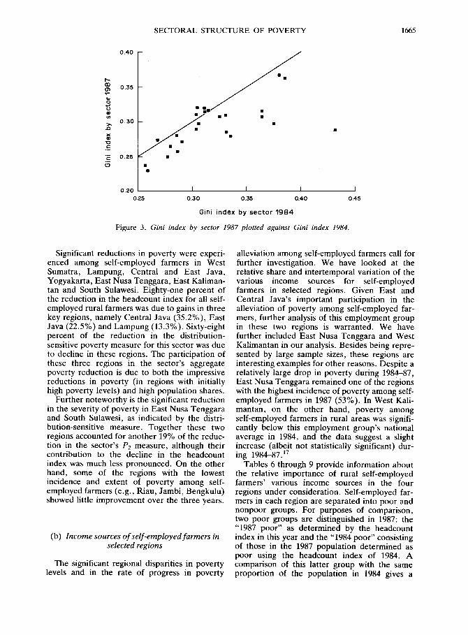
It can be seen from Table 3 that distributional changes helped alleviate poverty in 22 of the 28 sectors. In two sectors, urban farm laborers, and urban mine workers, poverty would have increased if the (negative) growth had been distributionally neutral, while it actually decreased. In these cases, over 100% of the actual change in poverty is attributable to improved distribution. But these sectors are unusual, and for the vast majority of sectors both growth and distributional changes helped alleviate poverty. What is striking, however, is the wide variation across sectors in the relative importance of these two factors. This trend is borne out clearly in Figure 3, which plots the 1987 Gini index against that for 1984 by sector.14 It can be seen that the Gini index fell in almost all sectors, but that the rates of improvement vary considerably across sectors. It is this variability across sectors in the shifts in distribution which accounts for the absence of a correlation between growth performance alone and the rate of poverty alleviation.

Given that intrasector changes in distribution generally alleviated poverty, one would expect the assumption of neutrality within sectors to lead to an underestimation of the aggregate reduction in poverty associated with the pattern of growth. It is also of interest to inquire into the magnitude of that underestimation for our data. The last row of Table 3 gives the estimated proportions of national poverty alleviation accountable to the sector growth rates in mean consumption assuming intrasector neutrality. Here we assume that both the actual growth rates in mean consumption and the changes in sector population shares are known; in practice, errors in assessing these will add to the imprecision in predicting the impact on aggregate poverty. We focus solely on the error due to incorrectly assuming neutrality within sectors. Since nearly 90% of the change in the headcount index is captured, the within-sector neutrality assumption

may be considered to provide a fair approximation of the aggregate change in the proportion who are poor (with known rates of change in means and population shares).15 The error is a good deal larger for the Pz measure, for which the neutrality assumption only picks up about two-thirds of the actual change in poverty. This disparity reflects the measure’s responsiveness to intrasector distributional shifts below the poverty line.

6. A CLOSER LOOK AT POVERTY IN THE FARMING SECTOR

(a) Regional dimensions

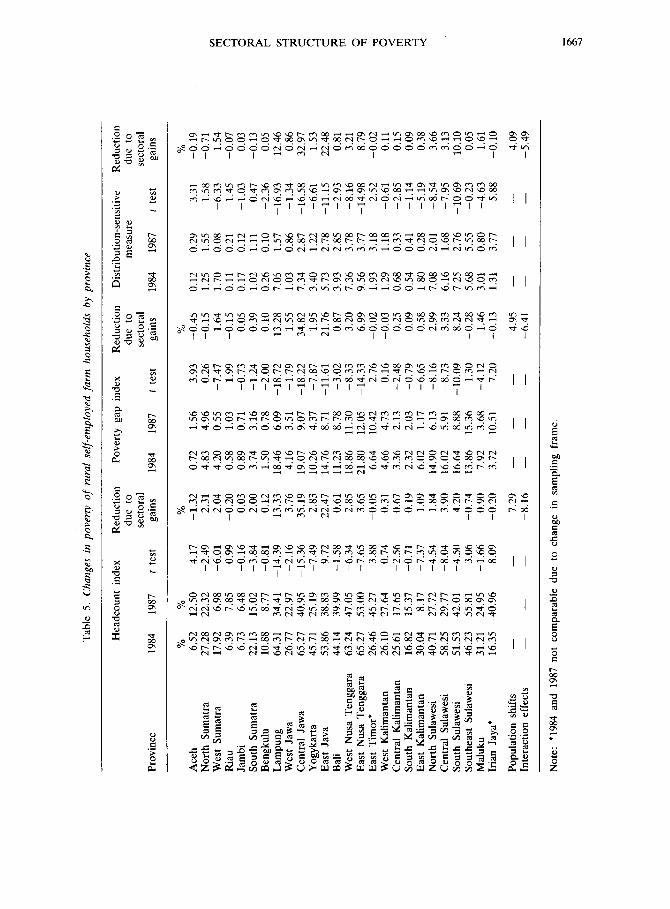
The importance of the rural farming sector in national poverty alleviation evident in Table 2 warrants further investigation. Tables 4 and 5 provide information about the regional distribution of self-employed farm households and the evolution of poverty among them. Regional disparities in average consumption, income and poverty levels of self-employed rural farmers are quite substantial, as are some of the changes in poverty during 1984-87. Average consumption by self-employed farmers decreased in eight out of 27 regions during the three-year period. Consumption decreases among self-employed farm households occurred solely in the Outer Islands.

Although average consumption of self- employed rural farmers fell in nearly a third of the regions, poverty in this employment sector increased with statistical significance in three regions only: Aceh, East Timor and Irian Jaya. Desirable intraregional distributional effects were clearly important in mitigating the effects of aggregate economic decline in the remaining regions where average consumption decreased. Note, however, that increases in the poverty measures among farmers in East Timor and Irian Jaya are probably due to changes in the SUSENAS sampling frame in these two regions during 1984-87, rendering the comparison doubtful. l6 The 1987 figures for these provinces are likely to be more accurate.

The spatial disparities in poverty incidence are marked. While poverty among self-employed rural farmers in Aceh, Riau, Jambi and Beng- kulu lay below 10% in 1984, over 50% of this employment group in Lampung, Central and East Java, East and West Nusa Tenggara and Central and South Sulawesi fell below the poverty line. Strong regional disparities were still prevalent three years later, although somewhat less pronounced.


Table 3. Sectoral growth and poverty alleviation

Income* source

Poverty alleviation (percentage) due to distributionally neutral

growth Headcount Poverty gap Distribution-sensitive

index index measure -

1. Farming

2. Mining

3. Industry

4. Construction

5. Trade

6. Transport

7. Finance

8. Services

National

Lt us

SE11 :” R

- 140.04 - 106.71 -88.12 88.38 85.33 81.59 78.45 88.24 85.47

118.83 76.01 72.46

L u -6.52 -3.45 -3.63 R 54.69 54.45 43.99

SE R 218.39 139.12 159.67

L u 111.79 146.88 130.69 R 137.75 97.75 112.68

SE U 71.41 82.82 56.00 R 65.66 59.53 58.59

L u 146.22 125.98 134.44 R 85.36 82.75 75.38

SE U 53.30 75.36 97.54 R 82.26 115.92 171.90

L u 106.24 102.25 R 43.41 54.58

SE U 100.84 75.34 R 64.17 71.93

L u R

SE U R

68.72 85.61 51.39

7.35

L u

L u R

SE U R

66.93 86.38 33.05

8.74

261.31

56.00 32.46 28.13 21.37

86.75

93.77

44.99 41.42 29.85 31.80

6X.02

91.29 67.87 73.03 73.38

76.02 81.85 51.36

7.45

203.70

53.86 47.13 33.42 34.25

67.81

*Sector definitions: 1. farming, husbandry, hunting and fishing. 2. mining and excavating. 3. industrial processing. 4. construction. 5. wholesale, retail, restaurant and hotel. 6. transportation, warehousing and communication. 7. finance, insurance, office rental, real estate and office services. 8. community services, social services and personal services.

tL = laborer/employee. $U = urban. §R = rural. j]SE = self-employed.


0.20 1 I I I I

0.25 0.30 0.35 0.40 045

Gini index by sector 1984

Figure 3. Gini index by sector 1987 plotted against Gini index 1984.

Significant reductions in poverty were experienced among self-employed farmers in West Sumatra, Lampung, Central and East Java, Yogyakarta, East Nusa Tenggara, East Kaliman- tan and South Sulawesi. Eighty-one percent of the reduction in the headcount index for all self- employed rural farmers was due to gains in three key regions, namely Central Java (35.2%), East Java (22.5%) and Lampung (13.3%). Sixty-eight percent of the reduction in the distribution- sensitive poverty measure for this sector was due to decline in these regions. The participation of these three regions in the sector’s aggregate poverty reduction is due to both the impressive reductions in poverty (in regions with initially high poverty levels) and high population shares.

Further noteworthy is the significant reduction in the severity of poverty in East Nusa Tenggara and South Sulawesi, as indicated by the distribution-sensitive measure. Together these two regions accounted for another 19% of the reduction in the sector’s Pz measure, although their contribution to the decline in the headcount index was much less pronounced. On the other hand, some of the regions with the lowest incidence and extent of poverty among self- employed farmers (e.g., Riau, Jambi, Bengkulu) showed little improvement over the three years.

(b) Income sources of self-employed farmers in selected regions

The significant regional disparities in poverty levels and in the rate of progress in poverty

alleviation among self-employed farmers call for further investigation. We have looked at the relative share and intertemporal variation of the various income sources for self-employed farmers in selected regions. Given East and Central Java’s important participation in the alleviation of poverty among self-employed farmers, further analysis of this employment group in these two regions is warranted. We have further included East Nusa Tenggara and West Kalimantan in our analysis. Besides being repre- sented by large sample sizes, these regions are interesting examples for other reasons. Despite a relatively large drop in poverty during 1984-87, East Nusa Tenggara remained one of the regions with the highest incidence of poverty among self- employed farmers in 1987 (53%). In West Kali- mantan, on the other hand, poverty among self-employed farmers in rural areas was significantly below this employment group’s national average in 1984, and the data suggest a slight increase (albeit not statistically significant) during 1984-87.”

Tables 6 through 9 provide information about the relative importance of rural self-employed farmers’ various income sources in the four regions under consideration. Self-employed farmers in each region are separated into poor and nonpoor groups. For purposes of comparison, two poor groups are distinguished in 1987: the “1987 poor” as determined by the headcount index in this year and the “1984 poor” consisting of those in the 1987 population determined as poor using the headcount index of 1984. A comparison of this latter group with the same proportion of the population in 1984 gives a

Tab

le

4.

Sum

mar

y da

ta o

f in

com

e ex

pend

itur

e of

se

lf-e

mpl

oyed

ru

ral

farm

ho

useh

olds

by

pro

vinc

e

Prov

ince

No.

of

%

of

Mea

n co

nsum

ptio

n G

row

th

Mea

n in

com

e G

row

th

sam

pled

se

lf-e

mpl

oyed

pe

r ca

pita

ra

te

per

capi

ta

rate

ho

useh

olds

fa

rm

popu

latio

n R

p./m

onth

t

test

R

p./m

onth

t

test

(3

yr

) 19

84

1987

19

84

1987

19

84

1987

19

84

1987

(%

)

Ace

h 92

1 78

5 N

orth

Su

mat

ra

931

942

Wes

t Su

mat

ra

672

577

Ria

u 61

0 60

8 Ja

mbi

42

9 49

8 So

uth

Sum

atra

85

7 90

4 B

engk

ulu

261

257

Lam

pung

1,

169

959

Wes

t Ja

wa

1,30

6 1,

115

Cen

tral

Ja

wa

2,01

1 1,

753

Yog

ykar

ta

654

508

Eas

t Ja

va

2,12

6 1,

940

Bal

i 84

7 60

6 W

est

Nus

a T

engg

ara

873

647

Eas

t N

usa

Ten

ggar

a 1,

210

3,53

6 E

ast

Tim

or*

129

292

Wes

t K

alim

anta

n 81

0 1,

026

Cen

tral

K

alim

anta

n 36

0 33

0 So

uth

Kal

iman

tan

730

561

Eas

t K

ahm

anta

n 31

4 35

5 N

orth

Su

law

esi

594

489

Cen

tral

Su

law

esi

378

342

Sout

h Su

law

esi

1,07

7 1,

127

Sout

heas

t Su

law

esi

973

340

Mal

uku

294

272

Iria

n Ja

ya*

252

631

2.75

5.

81

2.33

1.

69

1.38

3.

51

0.71

5.

57

12.3

7 18

.07

1.72

18

.67

1.84

2.

20

3.72

0.

03

2.48

1.

05

1.64

0.

62

1.77

1.

71

5.51

0.

97

1.79

0.

10

2.55

20

,398

18

,039

-5

.82

-11.

56

23,4

44

19,7

02

-5.0

7 -1

5.96

6.

30

14,1

74

16,3

99

7.54

15

.70

15,6

70

17,9

64

5.93

14

.64

2.09

16

,869

21

,290

9.

70

26.2

1 18

,454

22

,155

5.

80

20.0

6 1.

90

18,6

34

18,6

59

0.06

0.

13

21,7

93

20,6

57

-1.8

7 -5

.21

1.73

17

,665

18

,762

2.

21

6.21

20

,051

20

,120

0.

07

0.34

3.

92

15,9

63

18,7

53

7.50

17

.48

17,2

19

20,9

29

7.00

21

.55

0.85

18

,751

16

,952

-2

.88

-9.5

9 21

,736

19

,837

-2

.04

-8.7

4 5.

48

10,9

83

13,9

58

11.3

8 27

.09

14,1

76

17,4

28

2.94

22

.94

11.1

5 15

,884

16

,796

2.

56

5.74

18

,246

18

,365

0.

20

0.65

16

.31

10,7

63

13,4

97

13.3

4 25

.40

13,3

91

15,4

07

4.42

15

.05

1.45

12

,992

15

,126

5.

16

16.4

3 15

,684

17

,681

2.

85

12.7

3 18

.40

12,3

54

14,2

96

4.53

15

.72

15,0

99

16,8

40

4.09

11

.53

1.81

12

,556

13

,840

3.

24

10.2

3 16

,348

19

,236

2.

39

17.6

7 2.

18

11,0

66

12,8

41

5.02

16

.04

13,7

10

15,2

14

2.55

10

.97

3.80

10

,420

12

,092

8.

12

16.0

5 14

,073

16

,315

4.

12

15.9

3 0.

94

15,9

91

12,9

33

-4.0

4 -1

9.12

19

,338

18

,697

-0

.65

-3.3

1 2.

63

16,2

30

14,7

42

-4.3

2 -9

.17

17,3

12

17,3

85

0.12

0.

42

1.07

16

,809

16

,537

-0

.46

-1.6

2 19

,730

18

,524

-1

.40

-6.1

1 1.

46

16,8

20

15,8

27

-2.7

8 -5

.90

18,8

72

18,0

76

-0.9

0 -4

.22

0.83

15

,281

21

,098

8.

21

38.0

7 16

,892

24

,979

8.

14

47.8

7 1.

60

13,5

23

15,9

37

4.37

17

.85

16,1

71

21,8

81

4.62

35

.31

1.55

11

,262

15

,451

9.

06

37.2

0 14

,048

21

,766

5.

51

54.9

4 6.

07

12,4

96

13,0

06

1.78

4.

08

15,5

67

16,5

64

1.96

6.

40

1.20

12

,632

11

,339

-3

.64

-10.

24

15,9

29

15,3

10

-1.0

4 -3

.89

1.49

16

,013

15

,469

-0

.81

-3.4

0 19

,536

18

,093

-1

.48

-7.3

9 1.

25

18,0

84

13,8

61

-6.8

6 -2

3.35

21

,118

17

,402

-4

.51

- 17

.60

Not

e:

*198

4 an

d 19

87

not

com

para

ble

due

to

chan

ge

in

sam

plin

g fr

ame.

Tab

le

5.

Cha

nges

in

pov

erty

of

ru

ral

self

-em

ploy

ed

farm

ho

useh

olds

by

pro

vinc

e

Prov

ince

Hea

dcou

nt

inde

x R

educ

tion

Pove

rty

gap

inde

x R

educ

tion

Dis

trib

utio

n-se

nsiti

ve

Red

uctio

n du

e to

du

e to

m

easu

re

due

to

sect

oral

se

ctor

al

sect

oral

19

84

1987

t

test

ga

ins

1984

19

87

t te

st

gain

s 19

84

1987

t

test

ga

ins

%

6.52

27

.28

17.9

2 6.

39

6.73

22

.13

10.8

8 64

.31

26.7

7 65

.27

45.7

1 53

.86

44.1

4 63

.24

65.2

7 26

.46

%

%

-1.3

2 0.

72

1.56

2.

31

4.83

4.

96

2.04

4.

20

0.55

-0

.20

0.58

1.

03

0.03

0.

89

0.71

2.

00

3.74

3.

16

0.12

1.

50

0.78

13

.33

18.4

6 6.

09

3.76

4.

16

3.51

35

.19

19.0

7 9.

07

2.83

10

.26

4.37

22

.47

14.7

6 8.

71

0.61

11

.23

8.78

%

-0.4

5 0.

12

-0.1

5 1.

25

1.64

1.

70

-0.1

5 0.

11

0.05

0.

17

0.39

1.

02

0.10

0.

26

13.2

8 7.

05

1.55

1.

03

34.8

2 7.

34

1.95

3.

40

21.7

6 5.

73

0.87

3.

93

3.20

7.

36

6.99

9.

56

-0.0

2 1.

93

-0.0

3 1.

29

0.25

0.

68

0.09

0.

54

0.58

1.

80

2.99

7.

08

3.33

6.

16

8.24

7.

25

-0.2

8 5.

68

1.46

3.

01

-0.1

3 1.

31

4.95

-

-6.4

1 -

%

-0.1

9 -0

.71

1.54

-0

.07

0.03

-0

.13

0.05

12

.46

0.86

32

.97

1.53

22

.48

0.81

3.

21

8.79

-0

.02

0.11

0.

15

0.09

0.

38

3.66

3.

13

10.1

0 0.

05

1.61

-0

.10

4.09

-5

.49

Ace

h N

orth

Su

mat

ra

Wes

t Su

mat

ra

Ria

u Ja

mbi

So

uth

Sum

atra

B

engk

ulu

Lam

pung

W

est

Jaw

a C

entr

al

Jaw

a Y

ogyk

arta

E

ast

Java

B

ali

Wes

t N

usa

Ten

ggar

a E

ast

Nus

a T

engg

ara

Eas

t T

imor

* W

est

Kal

iman

tan

Cen

tral

K

alim

anta

n So

uth

Kal

iman

tan

Eas

t K

alim

anta

n N

orth

Su

law

esi

Cen

tral

Su

law

esi

Sout

h Su

law

esi

Sout

heas

t Su

law

esi

Mal

uku

Iria

n Ja

ya*

12.5

0 4.

17

22.3

2 -2

.49

3.93

0.

26

-7.4

7 1.

99

-0.7

3 -1

.24

-2.0

0 -1

8.72

-1

.79

0.29

3.

31

1.55

1.

58

0.08

-6

.33

0.21

1.

45

0.12

-1

.03

1.11

0.

47

0.10

-2

.36

1.57

-

16.9

3 0.

86

-1.3

4 2.

87

- 16

.58

1.22

-6

.61

2.78

-1

1.15

2.

85

-2.9

3 3.

78

-8.1

6 3.

77

-14.

98

3.18

2.

52

1.18

-0

.61

0.33

-2

.85

0.41

-1

.14

0.28

-5

.19

2.01

-8

.54

1.68

-7

.95

2.76

-1

0.69

5.

55

-0.2

3 0.

80

-4.6

3 3.

77

5.88

- - -

6.98

0.74

-6.0

1 7.

85

0.99

6.

48

-2.5

6

-0.1

6 15

.02

-3.8

4 8.

77

-0.8

1 34

.41

-14.

39

22.9

7 -2

.16

40.9

5 -1

5.36

25

.19

-7.4

9 38

.83

-9.7

2 39

.99

-1.5

8 47

.05

-6.3

4 53

.00

-7.6

5 45

.27

3.88

27

.64

17.6

5 15

.37

8.17

27

.72

-18.

22

-7.8

7 -1

1.61

-3

.02

Popu

latio

n sh

ifts

In

tera

ctio

n ef

fect

s

2.85

18

.86

11.3

0 -8

.33

3.65

21

.80

12.0

5 -1

4.33

-0

.05

-0.3

1 6.

64

10.4

2 4.

66

4.73

0.

67

3.36

2.

13

2.76

0.

16

-2.4

8 -0

.79

-6.6

5 -8

.16

-8.7

3 -1

0.09

1.

30

-4.1

2 7.

20

26.1

0 25

.61

16.8

2 -0

.71

-7.3

7 -4

.54

-8.0

4 -4

.50

3.06

-1

.66

8.09

-

0.19

2.

32

2.03

1.

09

6.02

1.

17

1.84

14

.90

6.13

3.

90

16.0

2 5.

91

4.20

16

.64

8.88

-0

.74

13.8

6 15

.36

0.90

7.

92

3.68

-0

.20

3.72

10

.51

7.29

-

- -8

.16

- -

30.0

4 40

.71

58.2

5 29

.77

42.0

1 55

.81

24.9

5 40

.96

-

51.5

3 46

.23

31.2

1 16

.35

- -

Not

e:

*198

4 an

d 19

87

not

com

para

ble

due

to

chan

ge

in

sam

plin

g fr

ame.

Tab

le

6.

Inco

me

sour

ces

of

rura

l sel

f-em

ploy

ed

farm

ers

in C

en

tml

Jaw

’

Yea

r G

roup

of

whi

ch

Anr

mal

%

of

Fa

rm

Bea

ns

& V

eget

able

s “C

ash

husb

andr

y Fo

rest

ry

&

Non

M

ean

popu

latio

n in

com

e G

rain

s tu

bers

&

fr

uits

cr

ops”

l/ &

da

iry1

Fi

sher

y hu

ntin

g fa

rmt

Wag

es

Cap

ital*

G

ifts

$ in

com

e

1984

19

84

poor

65

.3

5,14

9 2,

310

700

299

997

581

74

188

690

1.05

0 1,

379

361

8,62

9 19

84

nonp

oor

34.7

10

,081

4,

428

1,10

2 65

7 2,

139

1,31

8 25

6 18

1 1,

703

1 .I4

3 3,

506

1.75

7 18

,790

1987

19

84

poor

65

.3

5,81

5 2,

734

928

552

936

501

58

105

1,08

0 2,

028

1.27

4 12

4 10

,321

19

84

nonp

oor

34.7

12

.318

5,

525

1,13

7 66

8 2,

661

1,04

7 1,

214

67

2,72

0 2,

417

2,78

9 66

X

20,9

12

%

cont

ribu

tion1

984

poor

39

.36

25.0

4 13

.50

14.9

7 -3

.60

-4.7

2 -0

.93

~4.9

0 23

.05

57.8

0 -6

.22

- 14

.00

100.

Ou

to

incr

ease

in

19

84

nonp

oor

- 10

5.45

51

.69

1.65

0.

52

24.5

X

-12.

76

45.1

5 -5

.39

47.9

2 31

.75

-33.

78

-51.

33

loo.

(X)

tota

l in

com

e

1987

19

87

poor

41

.0

4,95

6 2,

326

865

482

812

342

44

85

792

1,96

0 1,

074

153

8,93

4 19

87

nonp

oor

59.0

10

,238

4,

660

1,09

5 66

9 2,

037

932

748

97

2,24

5 2,

304

2,30

5 42

4 17

,515

%

cont

ribu

tion1

987

poor

-6

3.33

5.

23

53.8

6 60

.00

-60.

43

-78.

22

-9.9

5 -3

3.83

33

.34

297.

87

-99.

82

-6X

.06

100.

00

to

incr

ease

in

19

87

nonp

oor

12.2

9 18

.17

-0.5

2 0.

92

~8.0

0 -3

0.27

38

.61

-6.6

2 42

.49

43.9

X

-94.

22

-104

.53

~100

.00

tota

l in

com

e

*All

figu

res

are

in

1984

ru

ral

pri

ces.

tN”n

farm

in

com

e in

clud

es

hand

icra

ft,

cotta

ge

indu

stry

, tr

adin

g,

tran

spor

tatio

n,

serv

ices

, co

nstr

uctio

n,

etc.

*C

apita

l in

com

e in

clud

es

inte

rest

s,

hous

e.

hall

and

equi

pmen

t re

ntal

s,

divi

dend

s,

pens

ions

, sc

hola

rshi

ps.

gran

t. lif

e m

sura

nce

and

othe

rs.

BG

ifts

refe

rs

to

the

bala

nce

of

gift

s re

cew

ed

and

gift

s m

ade.

Ir

Cas

h cr

ops”

in

clud

es

esta

te

and

plan

tatio

n cr

ops

(cof

fee,

cl

ove.

nu

tmeg

, pe

pper

, to

bacc

o.

rubb

er,

coco

nut,

suga

r ca

ne

and

“thc

rs).

IA

nim

al

husb

andr

y an

d da

iry

Incl

udes

ca

ttle

, po

ultr

y,

mis

cella

neou

s do

mes

tic

anim

als,

m

ilk

and

eggs

.

Tab

le

7.

Inco

me

sou

rces

o

f ru

ral sel

f-em

ploy

ed

farm

ers i

n Ea

st Jav

a

Yea

I G

rou

p

of

wh

ich

A

nim

al

%

of

FX

”l

Bea

ns

& V

eget

able

s “C

ash

h

usb

andr

y F

ores

try

&

Non

M

ea”

popu

lati

on

inco

me

Gra

ins

tube

rs

&

fru

its

UO

pS”

&

dair

y F

ish

ery

hu

nti

ng

farm

W

ages

C

apit

al

Gif

ts

inco

me

1984

19

84 p

oor

1984

non

poor

1987

19

84 p

oor

1984

non

poor

%

con

trib

uti

on19

84

poor

to

in

crea

se i

n

1984

non

poor

to

tal

inco

me

1987

19

87 p

oor

1987

non

poor

%

con

trib

uti

on19

87

poor

to

in

crea

se

in

1987

non

poor

to

tal

inco

me

53.8

4,

815

2,51

1 44

9 20

6 49

1 89

5 20

2 46

.2

10,7

89

5,14

8 1,

298

873

1,51

4 1,

242

664

53.8

5,

583

2,41

3 95

9 34

3 81

2 84

9 72

46

.2

12,4

13

5,94

4 1,

574

812

2,27

0 1,

399

359

65.6

1 -8

.35

43.5

1 11

.69

27.4

0 -3

.95

-11.

08

79.3

2 38

.87

13.4

9 -2

.99

36.9

1 7.

68

- 14

.89

38.8

5,

093

61.2

11

.048

96.9

4 21

4.89

2,20

3 5,

213

-107

.10

53.7

5

890

317

795

697

1,46

9 71

3 1,

921

1,35

9

153.

61

38.7

1 10

5.88

-6

8.79

14

1.68

-1

32.9

3 33

7.10

96

.75

64

126

294

81

-48.

07

22.7

0 -3

06.9

6 25

.50 61

50

136

55

6.39

0.

24

560

1,30

4 2,

120

213

9,01

2 1,

644

1,84

0 4,

353

618

19,2

44

556

1,64

4 2,

260

140

10,1

83

1,55

6 2,

570

3,97

1 78

2 21

,291

-0.3

5 29

.02

-11.

98

-6.2

6 10

0.00

-4

.32

35.6

6 -1

8.68

8.

02

100.

00

455

1,64

5 1,

985

121

Y ,2

99

1,37

4 2,

341

3,72

5 63

6 19

,123

-36.

51

118.

67

-47.

12

-31.

98

loO

.Cil

-2

23.8

6 41

4.85

-5

20.8

4 14

.95

-100

.00

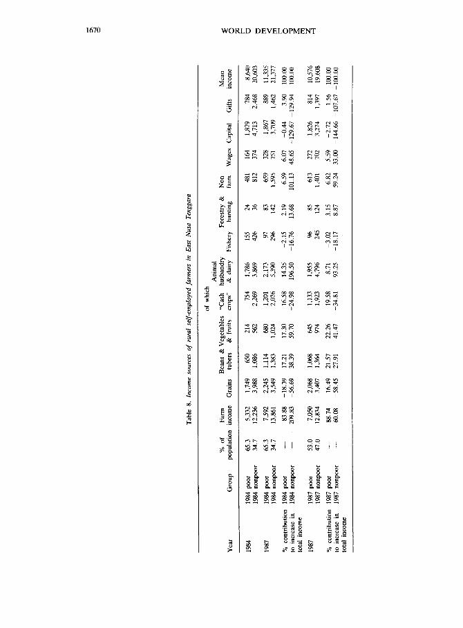
Tab

le

8.

Inco

me

sour

ces

of

rura

l sel

f-em

ploy

ed

farm

ers

in E

ast

Nus

a T

engg

ara

of

whi

ch

Ani

mal

%

of

Fa

llll

Bea

ns

& V

eget

able

s “C

ash

husb

andr

y Fo

rest

ry

&

Non

M

ean

Yea

r G

roup

po

pula

tion

inco

me

Gra

ins

tube

rs

&

frui

ts

crop

s”

&

dair

y Fi

sher

y hu

ntin

g fa

rm

Wag

es

Cap

ital

Gift

s in

com

e

1984

19

84

poor

65

.3

5,33

2 1,

749

650

214

754

1,78

6 15

5 24

48

1 16

4 1,

879

784

8,64

0 19

84

nonp

oor

34.7

12

,236

3,

988

1,08

6 56

2 2,

269

3,86

9 42

6 36

81

2 37

4 4,

713

2,46

8 20

,603

1987

19

84

poor

65

.3

7,59

2 2,

245

1,11

4 68

0 1,

201

2,17

3 97

83

65

9 32

8 1,

867

889

11,3

35

1984

no

npoo

r 34

.7

13,8

61

3,54

9 1,

383

1,02

4 2,

076

5,39

0 29

6 14

2 1,

595

751

3,70

9 1,

462

21,3

77

%

cont

ribu

tion

1984

po

or

- 83

.88

-18.

39

17.2

1 17

.w

16.5

8 14

.35

-2.1

5 2.

19

6.59

6.

07

-0.4

4 3.

90

100.

00

to

incr

ease

in

19

84

nonp

oor

- 20

9.83

-5

6.69

38

.39

59.7

0 -2

4.98

19

6.50

-1

6.76

13

.68

101.

13

48.6

5 -1

29.6

7 -1

29.9

4 lC

0.00

to

tal

inco

me

1987

19

87

poor

53

.0

7,05

0 2,

068

1,06

8 64

5 1,

133

1,95

5 96

85

61

3 27

2 1,

826

814

10,5

76

1987

no

npoo

r 47

.0

12,8

34

3,40

7 1,

364

974

1,92

3 4,

796

245

124

1,40

1 70

2 3.

274

1,39

7 19

,608

%

cont

ribu

tion

1987

po

or

- 88

.74

16.4

9 21

.57

22.2

6 19

.58

8.71

-3

.02

3.15

6.

82

5.59

-2

.72

1.56

10

0.00

to

in

crea

se

in

1987

no

npoo

r -

60.0

8 -5

8.45

27

.91

41.4

7 -3

4.81

93

.25

-18.

17

8.87

59

.24

33.0

0 -1

44.6

6 -1

07.6

7 -1

00.0

0 to

tal

inco

me

Tab

le

9.

Inco

me

sour

ces

of r

ural

self

-em

ploy

ed

farm

ers i

n W

est

Kal

iman

tan

i+

of

whi

ch

Ani

mal

9

%

of

Falll

l B

eans

&

Veg

etab

les

“Cas

h hu

sban

dry

Fore

stry

&

N

Oll

:: Y

ear

Gro

up

Mea

n po

pula

tion

inco

me

Gra

ins

tube

rs

&

frui

ts

crop

s”

&

dair

y Fi

sher

y hu

ntin

g fa

rm

Wag

es

Cap

ital

Gift

s in

com

e F

1984

19

84

poor

26

.1

;,704

3,

298

120

106

1,83

1 13

0 18

3 36

21

5 1,

043

1,72

5 61

8,

748

3

1984

no

npoo

r 73

.9

9,98

1 5,

434

235

214

3,00

8 25

9 58

6 24

5 1,

482

1,47

0 5,

179

95

18,2

07

z

1987

19

84

poor

26

.1

6,94

7 3,

536

132

269

2,63

0 31

24

7 10

3 44

2 65

9 1,

275

50

9,37

4

9 19

84

nonp

oor

73.9

10

,559

4,

612

195

652

3,91

1 19

8 59

5 39

7 88

7 2,

710

3,45

2 46

9 18

,077

%

cont

ribu

tion

1984

po

or

- 19

8.57

-3

7.97

1.

86

25.9

1 12

7.58

-1

5.81

10

.30

10.7

1 36

.24

-61.

26

-71.

83

-1.7

2 10

0.00

E

to

in

crea

se

in

1984

no

npoo

r -

444.

02

-631

.33

-31.

09

336.

54

693.

80

-46.

91

6.54

11

6.46

-4

57.0

5 95

1.86

-1

.326

.20

287.

37

-100

.00

tota

l in

com

e 2

1987

19

87

poor

27

.6

6,92

9 3,

534

129

267

2,59

6 31

24

9 12

3 46

2 66

3 1,

292

58

9,40

5 19

87

nonp

oor

72.4

10

,642

4,

635

197

661

3,95

2 20

1 60

1 39

5 88

8 2,

751

3,49

2 41

5 18

,248

z

%

cont

ribu

tion

1987

po

or

- 18

6.53

35

.91

1.32

24

.57

116.

50

-15.

12

10.0

6 13

.23

37.6

8 -5

7.81

-6

5.96

-0

.44

100.

00

IS

to

incr

ease

in

19

87

nonp

oor

- l&

02.3

9 -1

,937

.35

-92.

73

1,08

3.66

2,

288.

90

-140

.86

36.5

1 36

4.21

-1

,439

.68

3,10

7.37

-4

,091

.34

921.

25

100.

00

tota

l in

com

e

better indication of changes in income sources.” Note, however, that the relative importance of

from a booming rural nonfarm sector (Collier et al., 1988).

different income sources varies only slightly between these two groups of poor farm families,

There is a good deal of diversity across the four

but the growth rates of different incomes differ provinces in the sources of growth in farm

quite markedly. incomes. The main food crops (grains, beans and

In Central and East Java, poor self-employed tubers, fruit and vegetables) were quantitatively

farmers derived about 5560% of their income important to the growth of farm incomes in all

from farming (Tables 6 and 7). The proportion is four provinces. Only in West Kalimantan was

only slightly different for the nonpoor, and it is income growth from “cash crops” more impor-

generally higher. The share of farm income tant. In Central Java, average cash crop income

changed little over the period. Income sources of of the poor actually declined, although it in-

poor self-employed farmers in Java appear to be creased markedly in neighboring East Java (with a growth rate well above that of total farm

somewhat more diversified than earnings of the same groups in the two provinces in the Outer

income). This income source also grew rapidly in

Islands, where there was also a tendency for East Nusa Tenggara. In all except the latter

decreasing diversification over the period. In province, the growth in cash crop incomes was

West Kalimantan, poor self-employed farmers more important to the nonpoor, although the

earned almost three-quarters of their income poor may have gained indirectly through wage income growth, particularly in Java.

from farming in 1987, and this share had increased by nearly 10 percentage points over the

In sum, growth in wage earnings was very important to poor farmers in Java. A substantial

period. In East Nusa Tenggara they derived over two-thirds of their income from this source; the

increase in real wage earnings and a (more

share increased over the period, although less modest) increase in farming incomes were the

markedly than in West Kalimantan. most important contributors to higher incomes of

Wage earnings of self-employed farmers in the “1984 poor” self-employed farmers in Central Java. Wages were also an important source of

East and Central Java were substantially more important than in West Kalimantan (where the

income gains to the poor in East Java, although growth in nongrain farm incomes was more

contribution of this source declined) and East important there. In marked contrast to Java, Nusa Tenggara (where wage earnings were a wages mattered little to farmers in East Nusa negligible source of income for the poor). The Tenggara - gains to poor farmers in that relative importance of wages among the “1984 province arose from growth in a wide range of poor” in East and Central Java rose to over 16% and almost 20% respectively in 1987. They rose

crop and livestock incomes. Moreover, wage earnings were of decreasing importance in West

to 3% only in East Nusa Tenggara and dropped to 7% in West Kalimantan. In both Javanese

Kalimantan, where the modest income growth for the poor arose mainly from the “cash crops.”

provinces average wage earnings of poor self- Income from cash crops was also an important employed farmers grew at a significantly higher source of gains to the poor in East Java and East rate than earnings from any other source and Nusa Tenggara, although not Central Java, contributed markedly to the increase in total except possibly through employment growth in income. Average wage earnings of the “1984 that subsector. poor” farmers in Central Java almost doubled over the three-year period, thus contributing substantially to poverty alleviation among far- 7. CONCLUSIONS mers in this region. In West Kalimantan, where poverty among self-employed farmers barely Our main goal has been to describe the changed over the three years, wage earnings of sectoral structure of poverty in Indonesia in the the poor dropped significantly, as did their mid-1980s and how it evolved during the difficult relative importance. On the other hand, wage period of macroeconomic shocks and rapid ad- earnings of the nonpoor in this province in- justments. creased dramatically, although largely through a We have found that gains within the rural displacement of other sources. sector were quantitatively important to the coun-

As real wage rates appear to have changed try’s success at alleviating poverty during this little in either agriculture or the unskilled manu- period. In Indonesia, the highest concentrations facturing sector (World Bank, 1990a), this in- of poverty (both in terms of incidence and crease in real wage earnings in Java is likely to absolute numbers of poor) are found in the rural have been largely from employment growth. farming sector, and this sector accounted for Most of this employment growth probably came 70% of the reduction in our measure of the



severity of poverty during 198487. Gains to other sectors accounted for a further 25%) while 10% was due to population shifts, generally from rural to urban areas (the offsetting interaction effect between population shifts and sectoral gains was -5%).

The gains to the rural poor were largely due to growth in the sector’s mean income and consumption. At most 30% of the changes in the sector’s poverty measures was attributable to improved distribution within the sector. Over half of the gain to the rural farming poor is due to gains to the poor in two key provinces, Central and East Java. For them, gains to both farm incomes and wage earnings contributed to poverty alleviation, with the latter being particularly important in Central Java. The picture is much more varied among the Outer Islands, with increases in poverty among farmers in a few provinces, although rarely significant. In the two Outer Island provinces studied here in greater depth, East Nusa Tenggara and West Kaliman- tan, there is less sign of income diversification among farmers than in Java, and wage earnings were of little importance in poverty alleviation.

These results suggest that. features of the government’s adjustment program which favored rural areas, particularly on Java, were crucial to the evident success in maintaining the country’s momentum in alleviating aggregate poverty. Two such features have been suggested in recent discussions.

(a) There is evidence that the devaluations led to higher agricultural exports as well as (although less elastically than) manufacturing exports (Ahmed and Chhibber, 1989). Agriculture accounted for over half of the rise in nonoil exports during the adjustment period. It is not obvious a priori what effect a real devaluation would have had on poverty, since some of the poor may be net consumers of tradables, although it should be noted that Indonesia’s growth in agricultural exports was largely nonfood crops. Thorbecke (1990) reports general equilibrium simulations which suggest that In- donesia’s devaluations would have had favorable distributional effects. Our results indicate that where there were sizable gains in cash crop incomes, as in parts of Java and some of the Outer Islands, the poor participated in those gains.

(b) While it is not an issue our study can throw much further light on, it has been argued by the government and others that a serious attempt was made to protect fiscal allocations to programs which directly benefited the poor, including the rural poor. There is supportive evidence in the sectoral composition of public outlays over

the period (Ahmed and Peters, 1990; World Bank, 1990a; Thorbecke, 19901. For example, modest positive real growth in p ,blic investment in the agricultural sector was maintained, while public nonagricultural investment contracted. Among both routine and development expenditures, certain programs with probable benefits to the poor were sheltered, such as current transfers to the provinces and the more labor-intensive rural infrastructure projects, with the latter being encouraged in the attempt to expand rural employment opportunities during the adjustment period. The severest cuts in development expenditures tended to be in the more capital- intensive industrial and mining projects. It is likely, however, that the pattern of public sector retrenchment was not solely influenced by a desire to protect the poor during adjustment. More severe cuts in current government consumption spending (mainly wages for civil ser- vants) relative to investment in agriculture would probably have increased the rate of poverty reduction during the adjustment period; such a step would be consistent with the general equilibrium simulations of counterfactual experiments in Thorbecke (1990). Political economy considerations appear to have constrained the government’s attempts to buffer the poor from the costs of adjustment.

While the adjustment package undoubtedly helped, one should not underrate the role of Indonesia’s relatively favorable initial conditions for the adjustment period. The period of sus- tained and fairly equitable growth for a number of years prior to the adjustment period had created circumstances such that, by the mid- 1980s poverty would be quite responsive to further growth (Ravallion and Huppi, 1991). Conversely, the momentum of poverty alleviation could be maintained at lower growth rates. It can also be argued that much of the stimulus to rural infrastructure development from the late 1970s would have begun to yield substantial returns to the sector by the mid-1980s (Ahmed and Peters, 1990).

Indonesia’s poor are also thought to face relatively few constraints on their mobility across sectors (such as can arise through labor market inflexibilities and transport costs). This is particularly so in rural Java, which accounts for a large share of aggregate poverty in Indonesia. Ease of diversification in income sources will help the poor adjust to external shocks and macroeconomic policies, as World Bank (1990b, chapter 7), Walton (1990) and others have emphasized. We find indirect supportive evidence for this view in that the intrasectoral distributions were quite volatile during the adjustment period.


Under these conditions, the most important key to Indonesia’s success in poverty alleviation during this period may simply be that positive growth in mean private consumption was maintained, facilitated by an investment pause and external borrowing (Thorbecke, 1990; Walton, 1990). Initial conditions, and some ingredients of the adjustment package, helped assure that the poor continued to share at least proportionately in consumption growth. Without these fortuitous initial conditions the adjustment period would certainly not have yielded the same gains to the rural poor.

over the period clouded the relationship between sector growth and poverty alleviation. While distributional changes generally helped alleviate poverty, their relative importance varied enor- mously across sectors, and were probably associated with distributionally non-neutral workforce shifts. Distributions, however, were much more stable within regions, so that rates of poverty reduction and rates of growth were quite strongly correlated across provinces.

Although we find a strong negative correlation between levels of poverty and mean incomes across sectors at each date, there is no sign of such a correlation between growth rates and rates of poverty alleviation across sectors. The sectors which grew faster were generally not those where poverty was alleviated more rapidly. The afore- mentioned shifts in the intrasectoral distributions

Thus, although distributionally neutral growth in average consumption was clearly a strong driving force in the alleviation of aggregate

poverty (generally swamping the favorable effects of improved equity), its importance varied greatly across sectors of the economy. For future research, these results suggest that one should be wary of assuming that distributions are static

within sectors in an economy when analyzing the likely impact of the sectoral pattern of growth on poverty.

NOTES

1. For example, it has been argued that large farmers have gained proportionately more from the growth of nonfarm activities; see, for example, Thor- becke et al. (1990), which also references other work on this question.

2. Papanek (1988) estimates that real agricultural wage rates declined at about 1.7% per year in Central and East Java during 1982-87. The apparent inclusion of the last half of 1987 as the end date of Papanek’s series may tend to exaggerate the downward trend, as it coincided with a severe drought and unusually high rice prices. Concern has also been expressed about the particular price index used by Papanek, which is believed to have substantiallv overestimated the rate of inflation (notably in certain vegetable prices); see Ahmed and Peters (1990). Collier et al. (1988) do not find evidence of dechning’real wages in their study of 13 villages in the same provinces over a similar period, using a different deflator.

3. For examples of the use of this assumption, see the interesting counterfactual experiments on the effects of adjustment using applied general equilibrium models reported in de Janvry, Fargeix and Sadoulet (1990) and Thorbecke et al. (1990). Recognizing the potential problems of assuming static within-sector distributions, Thorbecke et al. avoid deriving the postreform household income distribution and poverty measures, but rather confine attention to distribution among socioeconomic groups.

4. Concern has been raised that the SUSENAS data may tend to underreport consumption. This problem is suggested by comparisons with the national accounts, although doubts have also been raised about accuracy

of the latter. It can be argued that any underestimation using the SUSENAS is more likely to be for the rich than the poor.

5. An urban-rural price differential of about 10% seems quite plausible for the poor, see for example, Rao (1984). and Ravallion and van de Walle (1991). It should be noted, however, that some past studies have assumed a higher differential between the urban and rural poverty lines. We interpret this as embodying relarivist poverty considerations, such that a higher real poverty line is used in urban areas. For further discussion see Ravallion and Huppi (1990).

6. Our earlier paper gives estimates of the difference involved in the poverty aggregates and their urban/ rural decomposition using the national accounts growth rate rather than the rate implied by the SUSENAS; see Ravallion and Huppi (1991).

7. More formally, one can write the FGT class of poverty measures as follows:

P, = B [(z-y,)lz]“/n

Y,<Z

where y, is the consumption of the ith person (estimated by the consumption per capita of that person’s household), z is the poverty line, n is population size and a is a non-negative parameter.

8. The ratio P,/Pn is sometimes called the “income- gap ratio,” and gives the proportionate distance of the mean consumption (or income) of the poor below the poverty line).

9. Having listed the 10 sectors and a residual category,

the respondent is asked: “Of the above, the major source of income is .” (Dari sumberpenghasilan di atas yang utama adelah). Note that the interpretation of “major” is subjective. This designation need not coincide with the largest income share in that year, although on inspecting the data the two generally coincide. Excep- tions may reflect an unusual year, or sluggishness in recognizing significant changes in income sources.

10. The table also gives the t-tests for a significant difference in the poverty measures between the years, . _ using the formulae for the standard errors of-these poverty measures given in Kakwani (1990). The test has a normal distribution.

11. The correlations are somewhat higher if one applies appropriate transformations to the poverty measures and means noting that the poverty measures are likely to be a decreasing convex function of the mean, and are also bounded above and below (as is clear from Figure 1 below); for example, the correlation between the logit transform of the headcount index for 1987 and the log of mean consumption is -.94.

12. The fitted values are given by

log[H/(l-H)] = -155.8 + 33.74logv (2.21) (2.43) - 1.83(logy)’ R*=.85 (-2.69)

where H denotes the headcount index and y is the sector’s mean income.

13. This estimate is based on a constant elasticity approximation; the point elasticities with respect to distributionally neutral growth of each poverty measure have been calculated for each sector in 1984, and these have been used to estimate the level of poverty that would have been observed in 1987 using the growth rates in Table 1. A more accurate method is to estimate the 1984 Lorenz curve for each sector, and use this to simulate the level of poverty that would have held in 1987 at the mean consumption or income for that year. Ravallion and Huppi (1990) use this method in similar calculations for the changes in aggregate poverty. It is computationally far more expensive, however, than


assuming constant elasticities, and will probably give a good enough approximation for our purposes.

14. A change in the Gini index is not sufficient for identifying whether distributional changes have benefited the poor, which also depends on the precise way in which the Lorenz curve shifts. The decomposition results in Table 3 are a better indicator. The popularity and ease of interpretation of the index, however, make it attractive for this illuslrative purposes.

15. If we had also assumed that population shares by sector had not changed over the period, the estimated proportions of the observed change in poverty accountable to the pattern of growth, assuming neutrality within sectors, are 89.06%, 68.46% and 68.00% for the headcount index, poverty gap index, and preferred measure respectively. It should also be recalled that we are assuming constant elasticities within sectors for these calculations. We do not know how much any deviations from that assumption are adding to the discrepancies between simulated and actual changes in poverty in Table 3, although we would be surprised if it is not tolerably small in the aggregate.

16. The SUSENAS sample in these two regions was greatly expanded in 1987. The 1984 sampling rate had been artificially low in rural areas of both provinces due to factors beyond CBS control.

17. We also constructed poverty profiles by sector of employment for these four provinces analogously to Table 2 for Indonesia as a whole. Sample sizes, however, were too small to be considered meaningful for most nonfarm sectors, particularly in the two Outer Island provinces. Comparing sectors with adequate sample sizes, the pattern for the Java provinces was quite similar to Table 2.

18. A comparison of the 1984 poor with the 1987 poor may be biased by differences among the poor in the composition of incomes; for example, the share of wages among the rural poor may increase solely because the “least poor” who crossed the poverty line were not wage laborers.

REFERENCES

Ahmed, Sadiq, and Ajay Chhibber, “How can Indone- sia maintain creditworthiness and noninflationary growth?” PPR Working Paper 291 (Washington, DC: World Bank, 1989).

Ahmed, Sadiq, and R. Kvle Peters, “Adiustment with poverty alleviation: Indonesia’s experience,” Back- around Paper to World Development Report 1990 TWashington, DC: World Bank’, 1990). -

Atkinson, Anthony B., “On the measurement of poverty,” Econometrica, Vol. 55 (1987), pp. 749- 764.

Collier, William L., Ir. Gunawan Wiradi, Soentoro, Makali, and Kabul Santoso, “Employment trends in lowland Javanese villages” (Jakarta: USAID, 1988).

de Janvry, Alain, Andre Fargeix, and Elisabeth Sadoulet, “Economic, welfare, and political consequences of stabilization policies: A general equilibrium approach,” Background Paper to the World Development Report 1990 (Washington. DC: World Bank,*1990). _ i -

Foster, James, and Anthony Shorrocks, “Poverty Orderings,” Econometrica Vol. 56 (1988), pp. 17s 177.

Foster, James, J. Greer, and Erik Thorbecke, “A class of decomposable poverty measures” Econometrica, Vol. 52 (1984), pp. 761-766.

Kakwani, Nanak, “Testing for significance of poverty differences with application to C&e d’Ivoire,” Living


Standards Measurement Survey Working Paper No. 62 (Washington, DC: World Bank, 1990).

Papanek, Gustav, F., “Changes in real wages: Employ- ment, poverty, competitiveness,” Research Paper No. 2, Development Studies Project (Jakarta: BAPPENAS/BPS, 1988).

Rao, V. V. Bhanoji, “Poverty in Indonesia, 197&1980: Trends, associated characteristics and research issues,” Mimeo (Jakarta: World Bank Resident Mission, 1984).

Ravallion, Martin. and Dominique van de Walle, “Urban-rural cost-of-living differentials in a developing country,” Journal of Urban Economics, Vol. 29 (1991), pp. 113-127.

Ravallion, Martin, and Monika Huppi. “Measuring changes in poverty: A methodological case study of Indonesia during an adjustment period,” World Bank Economic Review, Vol. 5 (1991). pp. 52-82.

Ravallion, Martin, Gaurav Datt, Dominique van de Walle, and Elaine Chan, “Quantifying the magnitude and severity of absolute poverty in the develop-

ing world in the mid-1980s;’ Background Paper to the World Development Report, 1940 (Washington, DC: World Bank, 1990).

Sen, Amartya, “Poverty: An ordinal approach to measurement,” Econometrica, Vol. 48 (1976). pp. 437-446.

Thorbecke, Erik, ‘*Adjustment, growth and income distribution in Indonesia,” Mimeo (Ithaca: Cornell University, 1990).

Walton, Michael, “Macroeconomic policies and poverty,” paper presented at the American Econo- mics Association Annual Meetings (Washington, DC: 1990).

World Bank, “Indonesia: Poverty assessment and strategy report,” World Bank Report No. 8034-IND (Washington, DC: World Bank, 1990a).

World Bank, World Development Report I990, Poverty (New York: Oxford University, 1990b).

World Bank, “Indonesia. Strategy for growth and structural change,” World Bank Report No. 7758- IND (Washington, DC: World Bank, 1989).

APPENDIX: SOME TESTS OF THE ROBUSTNESS OF THE RESULTS

(a) The choice ofpoverty line

At a poverty line of Rp. 11,000 monthly per capita consumption in urban 1984 prices, the headcount index of poverty dropped significantly in all employment sectors, but one, during 1984-87. We now ask how sensitive these results are to the exact choice of the poverty line and poverty measure.

In testing the robustness of our results to alternative poverty lines and poverty measures, we shall draw on the recent theoretical literature applying stochastic dominance arguments to the comparison of income distributions in terms of poverty measures (Atkinson, 1987; Foster and Shorrocks, 1988). We shall use two results from this literature. The first-order dominance condition. which states that if the cumulative distribution of consumption in 1987 lies nowhere above (and at least somewhere below) that for 1984 at all points up to the maximum conceivable poverty line, then all well- behaved poverty measures will indicate a reduction in poverty during 1984-87. If this condition does not hold, then some poverty measures and poverty lines will rank the two distributions differently from others. To re- solve this ambiguity, it may help to consider plausible restrictions on the range of admissible poverty lines. It can also help to consider a restricted class of poverty measures. Sen’s transfer axiom provides one such restriction. In particular, if we restrict attention to distribution-sensitive poverty measures, then the second-order dominance condition may prove useful. This condition states that if the area under the 1987 cumulative distribution function is nowhere greater (and somewhere less) than that under the 1984 distribution at all points up to the maximum poverty line, then poverty will have decreased according to any distribution sensitive measure satisfying certain mild conditions.

The first order dominance condition does not hold for 12 of the 28 sectors under consideration. Testing for

second-order dominance in these sectors, we found that dominance only failed to hold in three instances, namely for employees of the urban and rural manufacturing sector and for urban construction workers. All distribution-sensitive poverty measures and all poverty lines will thus indicate a decrease in poverty for 25 of the 28 sectors no matter where the poverty line is drawn.

(b) The choice of Welfare indicator

We are also concerned about robustness to the choice of welfare indicator. Two alternative indicators will be considered: a real consumption measure incor- porating an estimate of the interprovince differences in cost-of-living, and a measure based on the nonfood consumption share.

As we have noted, there is no ideal regional price deflator for Indonesia. Here we consider one possible contender, which we term the “spatial CPI.” The usual CPI is indexed to 100 at a common base date by dividing an estimated expenditure at each date by that for the base period. From the same data one can instead construct an index which uses a given date and place (such as February 1984 in Jakarta) as the base. If the expenditure data were for the same bundle of goods across all provinces then there would he a valid Laspeyres price index for making simultaneous spatial and temporal comparisons. The problem is that this condition does not hold, in that no attempt has been made to guarantee that one is costing the same bundle of goods. Nor is there any obviously sound basis for arguing that the adjustments to that bundle simply reflect local market conditions, such that there is a common underlying reference utility level. Nonethe- less, our alternative spatial CPI does at least incor-


porate information on spatial price differentials. Table Al gives the headcount index for each sector

based on the “spatial CPI.” It can be seen that deflation by the CPI for the poor and by the “spatial” CPI give quite similar results on the sectoral profiles of poverty for both dates. Clearly, the sectoral profiles average out a good deal of the spatial price variability.

A rather different welfare indicator is the nonfood consumption share, which is generally found to be a strictly increasing function of real income, and thus can be considered a valid welfare indicator. The main problem with this measure is that the function relating nonfood share to real income will vary according to other factors such as relative prices, demographic factors and tastes making nonfood share a noisy welfare indicator. Nonetheless, it is of interest to test the sensitivity of the sectoral profiles to a switch from the consumption based measure to nonfood shares.

We shall assume that a person is poor if their nonfood share does not exceed 25%. This point is in the range of commonly assumed cut-off points, and also gives an aggregate headcount index close to our poverty line. Table Al compares the headcount index based on nonfood shares with the headcount index based on total consumption. Again the correlation coefficient across sectors between the two measures is quite high (0.895 in 1984 and 0.804 in 1987). The two indicators, however, give quite different results on the movements over time and, indeed, the two do not always display a move in the same direction. While poverty appears to have dropped in all sectors but one according to the expenditure-based poverty measures (although with ambiguities at very low expenditure ranges in three sectors, as discussed above), the food- share based headcount index indicates an increase in poverty in nine sectors. In certain sectors, the two

Table Al. Alternative Headcounr Indices

Income source

1984 1987 Nonfood Nonfood

cPI* CPIS? share$. CPI CPIS share

Farming

Mining

Industry

Construction

Trade

Transport

Finance

Services

L u 41.51 R 53.01

SE U 35.37 R 43.91

L u 5.94 R 26.29

SE R 48.29

L u 9.94 R 23.82

SE U 16.80 R 35.57

L u 18.15 R 32.69

SE U 9.98 R 28.64

L u 8.54 R 33.79

SE U 9.97 R 26.75

L u 11.30 R 20.45

SE U 26.27 R 28.97

L u 0.38

L u 5.09 R 15.93

SE U 11.80 R 24.77

42.62 26.60 34.50 36.65 24.40 54.93 38.39 38.42 40.31 38.89 37.10 26.67 20.26 21.34 21.27 46.08 45.68 31.42 34.33 41.96

9.90 10.14 2.59 3.72 18.38 30.46 32.60 16.92 25.89 31.23 54.80 38.74 37.91 34.12 50.46

10.69 9.84 7.01 7.29 9.03 26.75 24.52 16.24 17.37 22.00 13.82 16.65 11.84 10.26 7.24 34.24 33.97 23.38 21.04 29.76

19.79 10.39 13.70 12.58 13.39 34.28 33.15 21.46 23.51 28.69

8.23 9.99 4.70 6.91 3.26 35.69 26.12 12.42 14.97 32.22

9.23 9.61 3.81 5.64 4.78 39.46 27.06 17.02 17.77. 28.70 IO.19 8.85 5.25 5.71 7.05 27.72 26.49 14.63 16.23 26.11

12.11 13.29 2.72 3.48 13.78 23.06 30.19 13.63 13.38 37.26 26.54 17.83 11.70 14.69 13.42 24.71 30.13 15.14 14.02 26.74

1.53 4.22 2.37 3.30 4.26

5.56 5.98 3.62 4.19 5.44 16.55 21.15 9.78 11.42 21.51 12.57 13.69 7.85 6.13 7.78 28.06 33.R6 20.75 20.85 26.46

*CPl headcount index: per capita consumption deflated by CPI for the poor. tCPIS headcount index: per capita consumption deflated by CPI taking into account spatial expenditure variations. $Nonfood share headcount index: Nonfood share poverty line: 25% of total expenditure.


measures also show rather large disparities between the sensitive to the choice of welfare indicator, with levels of poverty. significant increases in poverty indicated in a few

We can summarize our results as follows: the sectors using the nonfood share as the welfare indica- conclusion that poverty fell in almost all sectors is tor. The sectoral profiles at a given date are affected robust to the choice of a poverty line. It is more little by the choice of welfare indicator.

The Sectoral Structure of Poverty During an Adjustment ...

Documents

Transcript of The Sectoral Structure of Poverty During an Adjustment ...