The scope and organization of production: firm dynamics over the ...

180 Copyright q 2000, RAND

RAND Journal of EconomicsVol. 31, No. 1, Spring 2000pp. 180–205

The scope and organization of production:firm dynamics over the learning curve

Matthew F. Mitchell*

I introduce a Bayesian-learning model of the firm to account for a variety of empiricalfacts about firms. The many tasks the firm can undertake (the scope of the firm) areinformationally related, so that the firm can enjoy some economies of scope frominformation. The model predicts changes in firm size and its comovement with firmscope that are broadly consistent with the empirical evidence. It also provides anexplanation for the limits to the scope of the firm: the firm may lack information, or itmay be costly to communicate the information necessary to undertake many tasks.

1. Introduction

n It is now commonly known from panel data that firm size is highly variable, bothfor one firm over time and between firms at any point in time. The many empiricalregularities concerning the evolution of firm size have given rise to models where firmshave stochastic and persistent technological opportunities, such as Hopenhayn (1992),Jovanovic and MacDonald (1994), and Ericson and Pakes (1995). In this article Idevelop a model where these opportunities are the result of a specific mechanism, thefirm’s learning about its technology, and I explore the degree to which that learningmechanism can account for important features of firm dynamics.

The phenomenon of increased productivity (or lower costs) over the lifetime ofthe firm has been well documented (see, for instance, Argote and Epple (1990)). Theintent of this article is to develop a model of learning at the firm level and see to whatextent it can account for the key stylized features of the firm-dynamics literature.

The recent literature modelling the stochastic evolution of firms focuses only onthe overall size of the firm. Since there are useful data on the scope of firms and theplants they operate, my model differentiates between a scope margin and a scale mar-gin. Firms have access to a wide variety of tasks, of which they can choose a collectionto undertake. The optimal way of operating each task depends on an unknown param-eter.

This uncertainty poses some natural ways to explain the limitations to scope atany one firm. One reason a firm may choose to do some things but not others is that

* University of Minnesota; [email protected] article is a chapter of my Ph.D. dissertation at this University of Rochester. I thank my advisors,

Hugo Hopenhayn and Glenn MacDonald, for continuous advice and encouragement. I am also grateful forcomments from Kyle Bagwell, Jeff Campbell, April Franco, Jeremy Greenwood, Tom Holmes, Boyan Jov-anovic, Ron Jones, and an anonymous referee, as well as from numerous seminar and conference participants.Any remaining errors are my own.

MITCHELL / 181

q RAND 2000.

it does not have enough knowledge to efficiently undertake tasks that are intensive inthe area where its information is incomplete. In the model, some tasks are moreinformation-intensive, in the sense that any uncertainty about the unknown parameteris magnified. Consequently, the firm is limited in its ability to incorporate progressivelymore tasks in its operation.

The tasks are informationally related, so that knowledge about one task is portable,to an extent, to the operation of other tasks. The firm chooses which tasks to undertakeat a point in time, learns from that experience, and then chooses a new set of tasks tooperate the following period. Consequently, the scope of the firm changes over time.Firms can also choose the scale at which tasks are operated. As their expertise increaseson any one task, the scale of that task can rise with it. The model predicts relationshipsbetween the age of the firm, its size, and its scope that are broadly consistent withevidence from such studies as Gort (1962) and Salter and Ravenscraft (1979). It si-multaneously accounts for some of the salient features of the recent panel-study evi-dence on the evolution of firm size. In particular, it accounts for the two most importantfacts about the firm size-growth relationship: smaller firms grow faster than large firms,and smaller firms also have more variable growth rates. Evans (1987) and Hall (1987)show that these facts are robust even for sample selection and measurement errorcorrection.

The model’s ability to simultaneously account for a variety of features of the datais an important part of the article. In building a model of firm scope and scale, manythings will be modelled more explicitly than they have been in previous work (inparticular the learning problem, and learning across a variety of tasks), but, of course,many other features of the model are rather reduced form. The model’s ability to matchthe empirical facts, then, suggests that the learning mechanism is important and de-serves further attention. It also points to future work in that, to the extent that parts ofthe model are less explicit, further understanding of these elements can further con-tribute to an empirically meaningful model of the organization of production.

As mentioned, learning and expertise are the central theme of the modelling ex-periment. Learning has been suggested as a force behind the stochastic nature of thefates of firms. Here the firm is modelled as a Bayesian updating profit maximizer withincomplete information about the technology it operates. In that regard, it is similar tothe Bayesian-learning model of Jovanovic (1982). In that model, however, the firm’sproductivity is exogenously fixed; here, the firm learns how to organize productionmore efficiently over time. It is shown that the model presented here, aside from pro-viding a rationale for firm growth that differs than Jovanovic (1982), can also generatesome additional predictions that are consistent with firm data. Further, the informationalstructure here lends itself to the study of optimal firm scope. While the model focuseson the firm’s accumulation of expertise on one technology, the firm is allowed to choosefrom many potential outputs, termed tasks, to produce at each point in time. Conse-quently, the limited knowledge of how to do tasks provides a limitation on the scopeof the firm.

Since the learning process is motivated by incomplete information, the transitionfunction regulating the evolution of the firm’s productivity, and therefore employment,is a result of Bayes’ rule, rather than some arbitrary law of motion. Thus the modelcan provide an explanation for a wide variety of empirical implications, such as thepersistence of firm’s outcomes, that must be assumed as part of the law of motion inlearning treatments such as Ericson and Pakes (1995). On the other hand, the learningdoes not depend on the scale of operation, and is therefore very passive.

Uncertainty about the technology is modelled as an unknown ‘‘target’’ parameter.This part of the technology borrows heavily from recent work of Jovanovic and Nyarko

182 / THE RAND JOURNAL OF ECONOMICS

q RAND 2000.

(1995, 1996) and from earlier work by Wilson (1975) and Prescott (1972). The problemcan be viewed as one in which the firm must choose not only the amount of conven-tional inputs to hire, but also how to use those inputs. The choice of how to use theinputs can be viewed as a dial-setting problem. The firm chooses inputs and a dialsetting. The best dial setting is unknown to the firm. The firm makes its best guess atthe setting, observes the outcome, updates its beliefs about the optimal setting, andproceeds to the next period. The model is outlined in more detail in Section 2.

Section 3 investigates various forms of diminishing returns to scope. One possi-bility is that some tasks may be more difficult than others, in the sense of being moreinformation intensive. The difficulty of a task is modelled as sensitivity to the dialsetting. As tasks become more difficult, errors in the dial setting away from the bestsetting lead to a greater loss in output. One could say that surgery is more difficultthan carpentry in the sense that small cutting errors made in surgery lead to more direrepercussions than similar errors might in carpentry. For any fixed and limited amountof information, this increasing difficulty of tasks can lead to a limitation in the numberof tasks a firm operates. In other words, limited information in the face of growingdifficulty limits the scope of the firm. The model provides for an explanation of thedetermination of firm scope, which is vital to understanding the determination of firmsize.

The firm, then, chooses the tasks it undertakes, the scale of those tasks, and,importantly, the ‘‘way’’ it does the tasks, as indicated by its guess at the unknownparameter. In this regard, the model gives firms an important organizational role. Firmsuse their specialized knowledge, in the form of beliefs about the uncertainty they face,to organize production. How a firm goes about producing output, which might be calleda production technique, is a unique and important characteristic in my model.

Another possible reason for a limited scope is the possibility that many differentproduction techniques might be hard to unite in one firm. In informal language, a firmmight ‘‘lose focus’’ if it does too many tasks that involve disparate production tech-niques. Such losses might arise from a variety of coordination difficulties in imple-menting a wide variety of production methods within the same economic unit. Iformalize these reasons as a cost to disparate production techniques, so that the impli-cations of the ‘‘focus’’ of a firm can be explored. Limited focus can once again providea rationale for firms to operate a limited scope of tasks. There is a tradeoff betweenthe loss of focus from expanding scope and the inherent gains to be had from theinformational relationships between activities. The loss of focus is justified as a costof communicating knowledge within disparate tasks in the firm.

I introduce a notion of technological distance to formalize this idea of focus. Thedistance between tasks depends on the production techniques the firm chooses for thetasks. When tasks continually differ in terms of their most efficient technique, and theoperation of disparate techniques is costly, the firm again is limited in its scope. Thisis another way that the informational structure allows for an explanation of the limi-tations to scope that is unavailable when production simply maps conventional inputsto outputs.

Section 4 discusses the model’s predictions. I show that the model can explainseveral features of the relationship between firm scope and scale. The learning curvein the model generates naturally the valid prediction that firm growth is negativelycorrelated with firm size. The model also has reasonable predictions for the evolutionof average cost over the life of the firm. Moreover, the model suggests a rationale forthe persistent outcomes of firms and suggests some additional predictions that couldbe examined in the data.

MITCHELL / 183

q RAND 2000.

By combining the increasing difficulty of tasks introduced in Section 3 with thecosts of setting varied techniques, the model is able to generate employment patternsthat display variance across firms of the same age. Smaller firms not only grow faster,they grow more variably. The details are explained in Section 4.

2. The firm and its technology

n Consider a firm faced with many possible tasks to undertake with a given tech-nology. The firm produces output at each task it undertakes, and it must choose whichtasks to operate. The tasks are denoted s ∈ R1. The firm chooses a closed set P oftasks to undertake in the current period. The set P is the scope of the firm, that is, theset of different things the firm does. Output for task s is produced from some inputsxs. The ‘‘intensity’’ of task s is given by a constant-returns function f s(xs); for simplicity,let x ∈ R, so that the sole input can be thought of as labor and f can be written simplyas asxs.1

Not only does the firm have to choose which tasks to operate and at what intensity,it must also figure out how to best undertake each task. Firm management has signif-icant decisions to make beyond simply the hiring of inputs and the choice of tasks tooperate. The firm chooses a production technique qs ∈ R for each task. This techniquemight include organizational considerations such as the physical arrangement of thefirm’s inputs, the way to treat the inputs, or any other of the many management deci-sions that go on daily at a firm. For each task, the function hs(qs, u 1 e) defines howthe chosen technique qs affects the productivity for task s. The parameter u ∈ R isunknown and specific to the firm. The firm learns about the nature of its technologyas it learns u, and it can translate this knowledge into higher productivity by improvingits choice of production technique qs. Improvements in productivity owing to betterestimation of u can be viewed as ‘‘organizational capital,’’ in the sense that betterorganization of inputs (choosing qs more efficiently according to hs(qs, u 1 e)) is aninput into producing output. This capital is firm specific rather than match specific, asin the specification of Prescott and Visscher (1980). The e term reflects some normallydistributed mean-zero independent disturbance with variance s . Output for task s is2

e

ys(qs, u 1 e, xs) 5 hs(qs, u 1 e) fs(xs)g.

The firm’s production technique may be successful, or it may not, and that successaffects the productivity of the inputs hired for that task. For instance, one might leths 5 1 2 (s(u 1 e) 2 q)2. The production technique that maximizes expected produc-tivity for task s, then, is qs 5 su. Since the function hs depends on a single unknownparameter u for all the tasks, learning about one task enhances the firm’s knowledgeabout u, which in turn helps the firm operate other tasks. In that sense, tasks areinformationally related, and u is interpreted as a technology-specific parameter. Theorganizational choice qs can be interpreted, for instance, as the organization of a par-ticular vintage of capital on the shop floor, or as a management practice that allowslabor to be most efficient with the capital in place.

The choice of hs dictates the informational structure of the model. Jovanovic(1982) studies a model where there is a fixed unit measure of identical tasks and theinformational structure is hs 5 j(u 1 e), where the function j satisfies a variety ofregularity conditions. I shall focus on forms of hs such as the one in the previousparagraph, where u affects the optimal choice of qs and together they affect productivity.

1 All of the results extend naturally to the case in which x is a vector of inputs.


q RAND 2000.

This allows firms to improve their productivity through their lifetime and allows theinformation structure to potentially vary across s. Both of these facets of the infor-mation structure will have important implications, particularly in the firm’s choice ofscope P.

Another way to model informationally related activities would be to model eachtask as having its own unknown parameter drawn from some joint distribution withcorrelation between the unknown parameters for the various tasks. Dealing with mul-tiple unknown parameters, however, limits the tractability of the model. Here, analyticresults will relate the model to some data on firm dynamics. Using the single u has theadvantage of simplicity. The function hs does the work of mapping the single u intodifferent optimal production techniques across tasks, since it depends on the task s.

While the informational structure will have some built-in explanations for thelimitations to scope, it is less natural to find informational limits to scale. If the firmknows how to make a certain quantity of output with a set of tasks, inputs, and pro-duction techniques, then it is not clear, at least in this framework, what informationallimits keep the firm from replicating that procedure. Consequently, something else isneeded to limit the scale of the firm. The fact that the production function f (x) is takento the power g , 1 indicates the usual sort of span-of-control limitations to scale, asin Lucas (1978), which are not elaborated here.2 Output from the technology simplysums the output at all the tasks, and therefore output is given by

gh (q , u 1 e) f (x ) ds.E s s s sP

Given a wage rate w, input costs for the technology are simply

w ·x ds.E sP

The firm, then, chooses P and a set of inputs {xs}s∈P for all the tasks in the set P.The firm also chooses a profile of production techniques {qs}s∈P for the tasks it operates.Assume that, after realizing output, the firm also discovers, costlessly, the realized u 1 efor that period.3 The firm will be assumed to be a single-minded entity, so that we canavoid issues concerning the structure of management.4 Suppose the firm has beliefs mabout u represented by a normal distribution with mean m and variance s . The firm2

m

wishes to maximize the infinite sum of expected profits, given the beliefs m, discountedby the factor 1/(1 1 r), where r . 0 is the (fixed) interest rate. Denote the output pricefor the firm by p.5

Suppose that each firm in the industry draws its own u from a normal distributionwith known mean u and variance s . Under this assumption, there is no incentive to2

0

watch the results of others: all the relevant information about the aggregate distribution

2 There has, however, been a wide variety of articles focusing on this part of the firm’s problem.3 Of course, if hs is a one-to-one function in u 1 e, this is completely innocuous. However, forms that

are not one to one will be the focus here.4 The explicit informational structure introduced here allows for natural extensions to allow for the firm

to include many managers, each of which has his or her own beliefs and role in the decision process. Suchan extension is an interesting avenue for future research.

5 It is no loss to allow p and r to be time dependent. To concentrate on the role of the learning processin generating firm dynamics, the role of p and r changing over time will not be considered, so the firm canbe viewed as being a member of an industry in a stationary equilibrium.

MITCHELL / 185

q RAND 2000.

is given by u and s . This allows the model to focus on the effects of the firm’s own20

experience on learning.6 The firm updates the beliefs m optimally using Bayes’ ruleupon realizing u 1 e. Notice that since the observation is independent of any action,for instance the labor hire xs, the learning is passive. Throughout, the firm will be takento be the store of information. The internal structure of the information is left un-modelled, although a certain reduced-form for hs introduced below is meant to capturethe idea that information communication within the firm might be costly.

3. Diseconomies of scope: difficulty and focus

n Whenever there are decreasing returns to scale at the task level (g , 1), there isan economy of scope in the sense that spreading inputs over a larger set of tasksincreases output, other things equal. The nature of this model is that the informationstructure contained in hs can be used to introduce some balancing diseconomies ofscope. Two are introduced. The first is increasing difficultly of tasks, so that a firmwith limited information can only profitably enter into production of tasks that are‘‘simple’’ enough; undertaking hard tasks is decreasingly productive, and so scope islimited. The second is the idea that it may be hard for the firm to ‘‘focus’’ on a varietyof very different sorts of tasks, and therefore the firm must pick a limited set of tasksto undertake.

▫ Hierarchical difficulty of tasks. In a model with multiple tasks, it makessense to differentiate the tasks in some way. Why does the firm choose to do sometasks and not others? One possibility is that some tasks are more easily accom-plished than others. The challenge for the firm is figuring out which production tech-niques to employ, given the uncertainty about the parameter u. Consider the functionhs(qs, u 1 e) 5 1 2 (s(u 1 e) 2 qs)2. For tasks with a higher index s, the u 1 e termis magnified, making both the ‘‘target’’ choice of u and the noise term larger. For anyamount of knowledge, this will have the effect of increasing the expected disparitybetween qs and the target technique as s increases. Tasks with higher index s are moreinformation intensive.

The choice of inputs and techniques does not affect the realization of u 1 e. Thisis the sense in which learning is passive: no decision of the firm, for instance the laborchoice or the dial setting, has any effect on the evolution of beliefs. As a result, theeffect of any action is purely its effect on the current period’s output, so the firmchooses the inputs, as well as the scope P, to maximize current-period expected output.For the choice of qs, this is accomplished by setting qs 5 sEm(u) 5 sm. Em denotes theexpectation of u with respect to the beliefs m. Knowing the form of qs, we can turn tothe optimal (static) choice of scope and scale, knowing that for this formulation it isalso dynamically optimal.

Expected output for task s, when qs is taken to be the optimal sm, is

(1 2 s2(s 1 s ))a x .2 2 g gm e s s (1)

As was suggested earlier, any uncertainty about the true u, given by variance s , is2m

magnified by the s2 term.

6 Irwin and Klenow (1994) find that observing the firm’s own output is significantly more important tothe learning process than is learning from others. Adding learning from others would be a meaningfulendeavor, however. Foster and Rosenzwieg (1995) find significant knowledge spillovers in agricultural datafrom India.


q RAND 2000.

The dynamics of the beliefs m that define the firm are generated by Bayes’ rule,which means the model predicts the behavior of important firm variables. If we letas 5 1 for all s, then it is easy to characterize the solution to the firm’s problem at anypoint in time. The firm operates P 5 [0, b], where b 5 1/Ïs 1 s . The input choice2 2

m e

xs is ( pg /w(1 2 s2(s 1 s )))1/(12g). Expected output for tasks s, then, is given by72 2m e

g/(12g) 1/(12g)pg2 2 2y 5 (1 2 s (s 1 s )) .s m e11 2 2w

The mean m does not affect the choices of the firm besides qs, but s is relevant2m

to the labor and scope decision. Its evolution, if next-period belief variance is denoted(s )9, is given by Bayes’ rule as2

m

2 2s sm e2(s )9 5 . (2)m 2 2s 1 sm e

Notice that the variance of the firm’s subjective beliefs falls through time. To be con-sistent with the information the firm has at the beginning of its life, let s 5 s in the2 2

m 0

first period of the firm’s existence. Here, m doesn’t enter, since the size of u doesn’taffect firm success. This is the opposite of Jovanovic (1982), where the size of u isprecisely the object of interest in determining firm’s productivity. Later I develop amodel that allows for ‘‘selection,’’ in the sense that some firms draw u’s that areinherently more productive while they maintain the learning structure of increasingproductivity through improvements in their choice of qs.

The fact that the firm operates a limited set of tasks is not restricted to the casewhere as 5 1. Notice that if either s or s is greater than zero, then the first part of2 2

e m

(1) is negative for sufficiently large s. In other words, if the firm has meaningfulincomplete information about the unknown parameter u (so that s is positive), then2

m

sufficiently information-intensive tasks cannot be accomplished with positive expectedreturn. The firm will not undertake these difficult tasks, given their limited information.In the language of the model, we have the following.

Proposition 1. If hs 5 1 2 (s(u 1 e) 2 qs)2 and either s or s is positive, then the2 2e m

scope of the firm, P, is bounded.

Information limits the scope of the firm. In this way, information is a limitationto scope along the lines of Lucas (1978), but it arises as a consequence of the uncer-tainty in the decision problem facing the firm. Firms have limited information, andsome tasks are so information intensive that it is not profitable to operate them withoutmore certainty about the appropriate techniques {qs} to use.

▫ Communication, technological distance, and loss of focus. One force restrictingthe scope of firms is limited information. In addition, a firm must also communicateinformation to the workers who undertake production. This subsection considers amodification of the earlier model where a firm’s limited ability to communicate itsknow-how, and not the inherent difficulty of the tasks, limits its ability to diversify.

7 Total output is obtained by integrating ys across tasks; the solution to this integration is quite com-plicated. Since it is easy to analyze the scale of each task and the overall scope of the firm with simpleformulas that give unambiguous implications for total size, total output is not calculated except for the casewhere g 5 .5, which is discussed in the next section.

MITCHELL / 187

q RAND 2000.

When we combine the two limits to scope, the model is able to generate variance inthe distribution of employment within a particular age cohort.

The role of ‘‘ focus.’’ There are many reasons why implementing different productiontechniques may be costly to undertake within a single firm, and as a result the scopeof the firm may be limited.8 Often, the manager of the firm, who may be endowedwith the knowledge given by beliefs m, is not the one directly involved in producingthe output. Communicating the production techniques for each task to the workersmight be costly, since it might require the manager’s time or the hiring of some sortof foreman. This is the sense in which costly communication can make undertakingvarious tasks costly. Sometimes, disparate production techniques are hard to integrateinto one production process. If the production technique for one task involves toxicchemicals and that for another task produces food, the firm will need to go to speciallengths to separate the two tasks.

The way to incorporate this in the model is to use q as a measure of distance ordiversity in activities or techniques. Letting optimal techniques become farther apartas tasks become farther apart along the real line and adding a cost of setting diversetechniques forces the firm to ‘‘focus’’ on a subset of the available activities, despitethe decreasing returns to any one task. To do tasks productively, q will need to befarther and farther apart as the distance between any two tasks increases.

The idea of a distance between two methods of production has appeared in manyrecent formalizations of learning. In Jovanovic and Nyarko (1996), new technologiesinvolve learning a new u. How close the new u is to the old one plays an importantrole in the adoption of the new technology, since that ‘‘closeness’’ reflects how easilyknowledge can be transferred to the new technology. In Auerswald et al. (1998), anytwo processes for producing output have an inherent, exogenous distance between them.In their framework, it is assumed that firms jump from the current process to a‘‘nearby’’ process. Here, technological distance is in terms of the different productiontechniques {qs} used by the firm.

Modelling focus. Since this subsection is concentrating on the role of firm ‘‘focus,’’ itis reasonable to want to exclude the effects of increasing difficulty of tasks. Considerthe form hs(qs, u 1 e) 5 1 2 (s 1 u 1 e 2 qs)2. As s increases, the best productiontechnique increases. In that regard, tasks differ. However, errors in setting qs are notmagnified as tasks grow more complicated; all tasks are equally difficult. Assume, onceagain, that f s is identical across tasks.

All the possible reasons for the costs of disparate production techniques will beput under the category of firm focus. Firms that focus on similar production techniquesavoid costs associated with ‘‘loss of focus’’ when a wide variety of techniques aresimultaneously employed by one firm. For a profile {qs}, the costs are

g 2C({q }) 5 f f (x ) (q 2 q ({q })) ds,s E s s s sP

where, letting m(P) denote the Lebesgue measure of P,

8 Among others, Rotemberg and Saloner (1994) explore the microfoundations of the costs of imple-menting a broad range of activities in an incomplete contracting framework.


q RAND 2000.

q dsE sP

q ({q }) 5 .s m(P)

Firms pay a cost for setting techniques away from the average technique q. This canbe viewed as the technological distance between techniques. The firm can implementq costlessly, for instance by distributing some sort of costless flyer or announcementto its employees, or because the employees are all doing the same thing and can easilysee what technique to use from observing others around them. In that case, there is nodistance between the techniques, so the distance cost is nothing. When the firm focuseson a production technique, it avoids the distance cost. Techniques far from the averagerequire special implementation costs, including communication of the technique to em-ployees and perhaps some special production costs in incorporating this unusual tech-nique. The cost is increasing in the ‘‘intensity’’ f s(xs) of the task, and it depends onthe constant f, which signifies how flexible the technology is to disparate productiontechniques. This cost represents losses due to what might broadly be called ‘‘loss offocus’’ as the firm expands the variety of things that it does.

To make the focus cost important, suppose that the input xs must be equal acrossall tasks incorporated in P. The idea is that each ‘‘production run’’ involves a fixed,constant amount of each task in P. To expand scale, we can increase the number ofruns, which increases inputs x identically across all tasks. The firm can still choosewhat tasks to do in each production run, as well as the overall scale of the operation.The importance of this assumption is that without it, firms could operate tasks at asmall scale simply to manipulate their average task q, and not for the profitability ofthe task itself. This leads to two problems. First, calculating the optimal qs and xs

becomes very difficult because of the effect each has on all the other tasks. Second, itmay be that the firm wishes to operate a great many tasks at a small scale so as tomanipulate q, but the tasks directly contribute almost nothing to firm output. For study-ing the scope of the firm, the inclusion of these ‘‘nothing’’ tasks seems uninteresting.Changing the definition of q above to weigh each qs by f s(xs)g does not solve theproblem of firms operating tasks for indirect benefit. The impact, in terms of overallprofits, of the change in q by adding an additional task is weighted over all the othertasks, since q enters into all of them and therefore may be large even if the change inq is itself small.

Here, the distance between different production methods, and the cost generated fromthe differences, depends on the disparity between how each technology is operated, asdescribed by the production technique qs. Technological distance plays a role in that dif-ferent types of production, in the model, are hard to combine at one location. Unlike othernotions of distance, the one I use here refers to differences in how a firm chooses tooperate a technology. The distance between techniques is chosen by the firm, not assumedby the model. What is assumed by the model is the distance between potential techniquesq and the interaction between q and s in the function hs. The technique that minimizesexpected differences from s 1 u 1 e is moving farther and farther away as s increases.

Solving the firm’s problem. Consider the case where as 5 1 for all s. Total output, netof focus costs, is

g 2 gh (q , u 1 e) f (x ) ds 1 f (q 2 q ) f (x ) ds. (3)E s s s s E s s sP P

Let X denote the total amount of inputs employed by the firm; since xs is taken to be

MITCHELL / 189

q RAND 2000.

a constant x in this subsection, X 5 xs ds 5 x ·m(P). Factoring out the f s(xs)g in (3)#P

and replacing xs with X/[m(P)] yields

gX2f h (q , u 1 e) ds 2 f (q 2 q ) ds .E s s E s1 2 1 2m(P) P P

Taking advantage of the homogeneity of f , net output can be rewritten as

2h (q , u 1 e) ds 2 f (q 2 q ) ds E s s E s

P Pg Y(X, P, {q }) 5 f (X) . (4)s gm(P)

Input costs are w ·X. Notice that the optimal choice of P and {qs} is independent of,and can be calculated separately from, the choice of X.

In general, finding the optimal {qs} is difficult, since it lies in an infinite-dimensional space. The following lemma shows how the quadratic distance cost allowsfor a simple form of the solution.

Lemma 1. Suppose hs 5 1 2 (s 1 u 1 e 2 qs)2. Then for any P, there is an optimaltechnique profile of the (linear) form

1 fq 5 (s 1 m ) 1 q ({q }). (5)s s1 1 f 1 1 f

Proof. Consider the function

2p̂(P, {q }, t) 5 h (q , u 1 e) ds 2 f (q 2 t) ds. (6)s E s s E sP P

When t 5 q({qs}), (6) is the firm’s objective in choosing {qs}. By Fubini’s theoremand the independence of the objective across s for a given t, the problem of

Em( (P, {qs}, t)) can be solved by computing the solution ofmax p̂qs

2max E (h (q , u 1 e) 2 f(q 2 t) ) (7)m s s sqs

for each s. Standard maximization shows that the solution to (7) is of the formin (5). Consequently, for any {q̃s}, we can construct a {qs} of the form in (5) with

(P, {qs}, q(q̃s)) $ (P, {q̃s}, q(q̃s)). Now consider the problem of maxt Em( (P, {qs}, t)).p̂ p̂ p̂Again, by standard techniques, it is easy to show that the solution is t* 5 q({qs}).Consequently, (P, {qs}, q(qs)) $ (P, {qs}, q(q̃s)) $ (P, {q̃s}, q(q̃s)), and {qs} ofp̂ p̂ p̂the form in (5) dominates {q̃s}. Q.E.D.

Suppose, without loss of generality, that the first task the firm incorporates is s 5 0.Under the normalization that the firm incorporates task 0 first, it chooses P 5 [0, b],and, using Lemma 1 to calculate {qs}, b can be calculated as


q RAND 2000.

Ï1 1 f Ï1 2 g2 2b 5 2Ï3 Ï1 2 s 2 s .m eÏf Ï3 2 g

So the productivity term multiplying f (X)g is

22g 12g 2 2 32g 12g 12g 12g 2(32g)A* 5 2 Ï3 (1 2 s 2 s ) (1 1 f) f (1 2 g) (3 2 g) .m e

The optimal scale of X can be calculated from first-order conditions as (gpA*/w)1/12g.Under the functional form chosen for hs, tasks are progressively more and more

dissimilar. This is formalized by the fact that the optimal production technique s 1 mrises in s. To do progressively more tasks effectively, each new task’s technique mustbe farther and farther away from the average. Eventually, the technique is either so faraway from the average, or so far away from the ‘‘best’’ technique s 1 m, that the firm’sexpected gain from adding that technique to its production runs becomes negative.Consequently, we have the following.

Proposition 2. Suppose hs 5 1 2 (s 1 u 1 e 2 qs)2 and f . 0. Then the scope ofthe firm P is bounded.

Proof. Consider the second term in (4). To keep hs(qs, u 1 e)ds from becoming#P

negative and hence the contribution of tasks s to be profit reducing, qs can never fallbelow s 1 u 2 1. However, any profile that does not fall below s 1 u 2 1 creates anarbitrarily large cost f (qs 2 q)2 ds for some task as s → `. Since hs(qs, u 1 e) # 1,#the cost eventually dominates, and the second term of (4) becomes negative for large s.Q.E.D.

Larger scope of production reduces focus. This tradeoff between informationaleconomies of scope and diseconomies from the loss of focus leads to a limitation onthe scope of the firm. It would also hold if the scale of each task could vary freely buthad to be operated at some fixed overhead amount o, so that each task had to be doneat some minimum scale.

4. Empirical implications for firm dynamics

n The model presented above provides some reasons for the limits on the scope offirms. The implications of the model can be elaborated and compared to some featuresof the data. Specifically, I consider scope, scale, and cost movements. Scale is takento be measured as labor input; this is common in the empirical literature, and in themodel there is a one-to-one mapping between labor input and expected output (or, bythe unbiasedness of Bayes’ rule, average output across many firms at a given state) fora given level of knowledge. Unless otherwise noted, the model is that of hierarchicaldifficulty of tasks. The model of focus has similar predictions. At the end of this sectionI consider a model with both increasing difficulty and cost of focus.

▫ The scope of firms. Two important regularities concerning the scope of the firmemerge from the work of Gort (1962) and Salter and Ravenscraft (1979). First, biggerfirms tend to be more diversified. Second, larger firms tend to also operate eachactivity at a larger scale then do smaller firms. In the model with hierarchical difficultyof tasks, this is a natural result. The updating equation (2) implies that s declines as2

m

the firm gets older. Both scope P 5 [0, 1/(s 1 s )] and the firm’s labor hired at task2 2m e

MITCHELL / 191

q RAND 2000.

s, xs 5 ( pg /w(1 2 s2(s 1 s )))1/12g, rise through time as the firms variance s de-2 2 2m e m

creases. Older firms are larger and operate more tasks, operate at a larger scale, andoperate a given task at a larger scale because their knowledge, embodied in a lowers , allows them to do more difficult tasks efficiently. Older, knowledgeable firms are2

m

bigger and involved in more things by virtue of their accumulated experience as mea-sured by lower variance about the unknown parameter

Another feature of the model that is consistent with both casual empiricism andsome studies of particular industries is that firms commence production with a subsetof the tasks they eventually undertake. For instance, Shaw (1995) suggests that newsteel plants start up doing only a few of the tasks they intend to eventually do, learnfrom experience, and then add tasks. This is exactly the sequence of events the modelpredicts: not only does P rise in terms of its measure, but also Pt , Pt11. Along thescope margin, the model naturally predicts that firms move from the simplest tasks tomore complicated ones. A different Bayesian-learning explanation for this progressionis presented in Jovanovic and Nyarko (1997). In their framework, agents start withsimple activities because simple activities offer better learning possibilities. In the mod-el above with progressively more complicated tasks, firms start with simple activitiesbecause the loss from making bad decisions on more complicated tasks is exaggerated.Firms wait until they have further knowledge before undertaking the more difficulttasks.

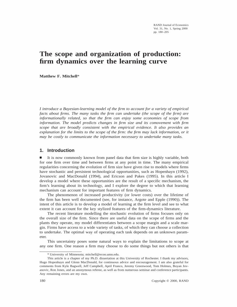
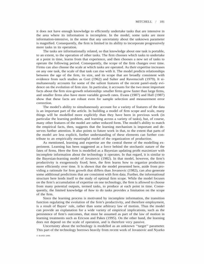
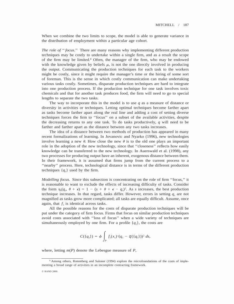
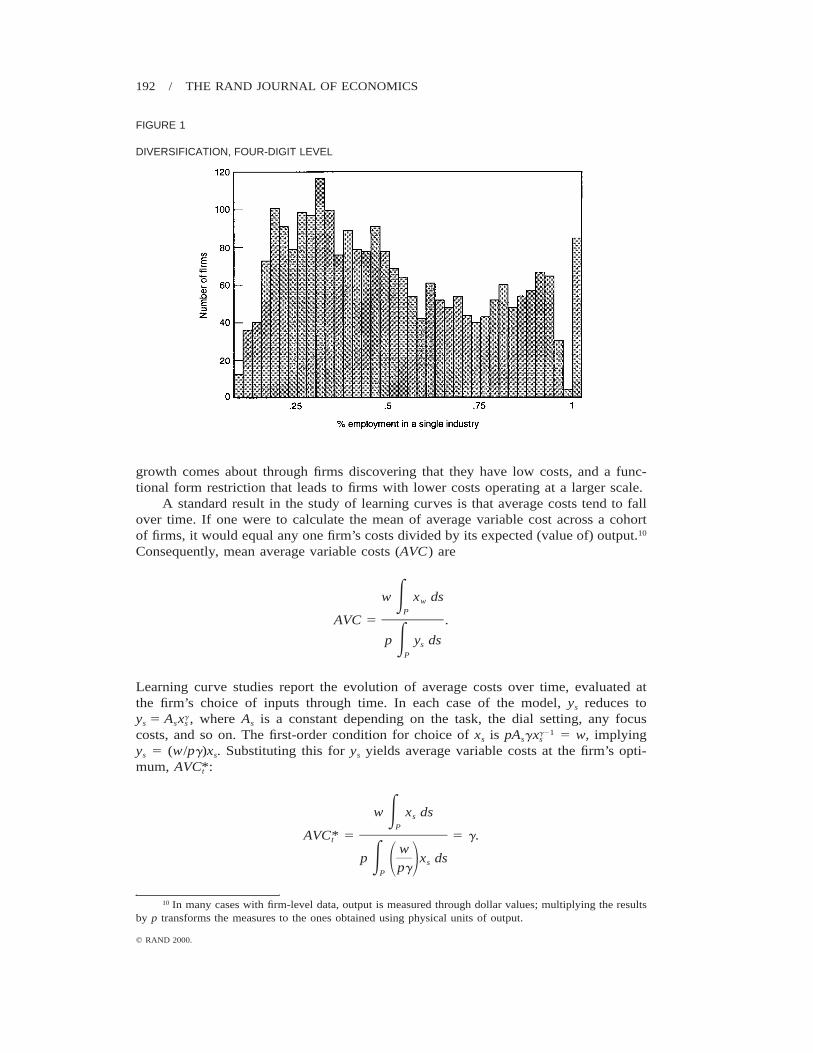
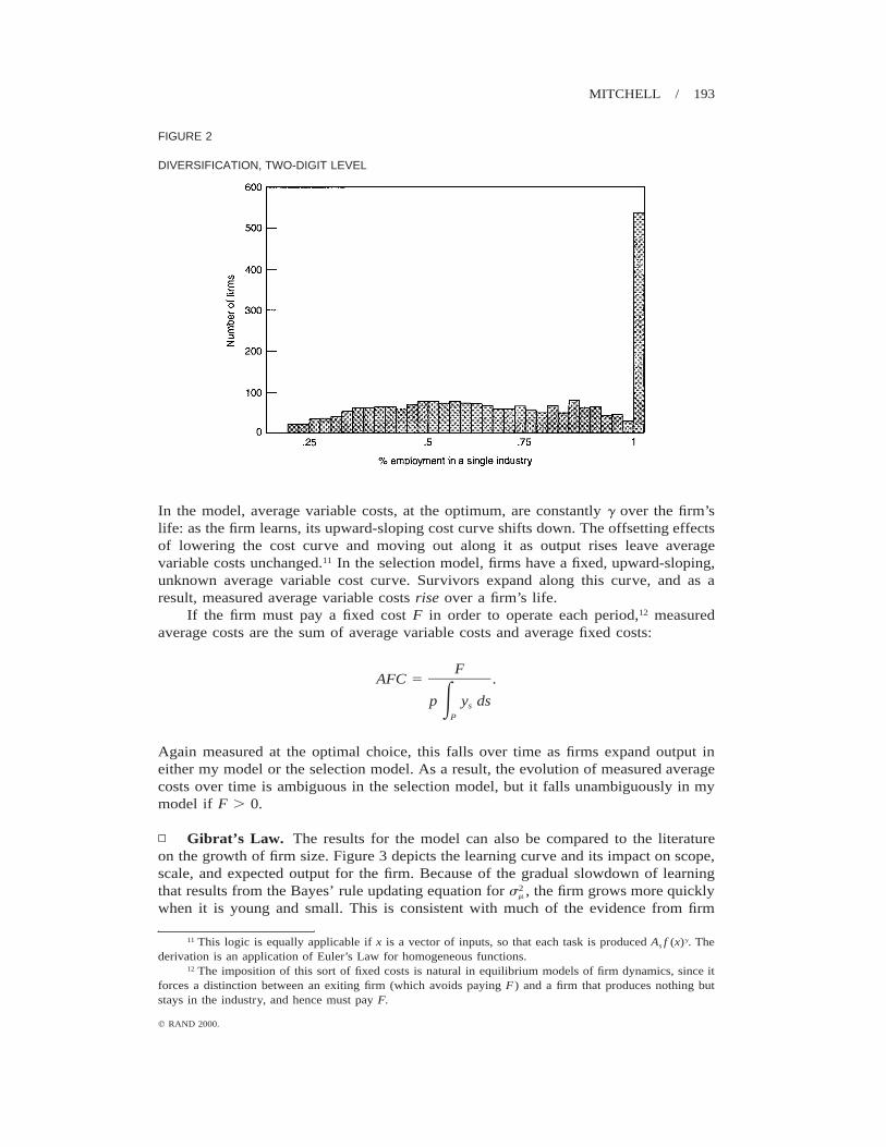
It should be noted that as a model of diversification, this model points to a learningmechanism driving diversification into related tasks as the firm accumulates informa-tion, since the relevant scope-determining parameter is knowledge about a parameteru common to all tasks. Diversification into similar tasks appears to be a quantitativelyimportant element of diversification. Figure 1 is a histogram of diversification datataken from a CompuStat manufacturing sample studied by Cardinal and Opler (1995).The horizontal axis is defined by the fraction of a particular firm’s employment thatresides in its largest (as measured by employment) four-digit Standard Industry Clas-sification (SIC) code line of business. At this level of disaggregation, only a very smallfraction of firms (the rightmost bar—about 2%) are nondiversified in this sample. Infact, many firms have less than half of their employment in any one four-digit SICcode, as seen by the bars to the left of .5. Figure 2 repeats the exercise, this time usingthe less aggregated two-digit SIC codes. More firms are nondiversified at the two-digitlevel, significantly more than if firms were choosing their four-digit product line choicesrandomly. This suggests that related diversification is important: The choice of industryis not random across four-digit industries but rather is clustered in two-digit industries,suggesting that the sort of learning mechanism proposed has something relevant to sayabout diversification.9

▫ Average costs and the learning curve. Aside from the introduction of a scopemargin, a difference between my model of firm learning and the most popular learningmodel used in the study of firm dynamics, the selection model of Jovanovic (1982),comes in the evolution of productivity (and, as a result, average costs) over the learningcurve.

The selection model concerns firms learning their (exogenously fixed) productivity.As a firm learns its productivity, it learns the optimal amount of inputs to hire tominimize per-unit costs. In the formulation above, productivity is not fixed but tendsto rise as firms learn how to operate their technology. In Jovanovic’s selection model,

9 Certainly, examples of unrelated diversification can be found, relying on other explanations.


q RAND 2000.

FIGURE 1

DIVERSIFICATION, FOUR-DIGIT LEVEL

growth comes about through firms discovering that they have low costs, and a func-tional form restriction that leads to firms with lower costs operating at a larger scale.

A standard result in the study of learning curves is that average costs tend to fallover time. If one were to calculate the mean of average variable cost across a cohortof firms, it would equal any one firm’s costs divided by its expected (value of) output.10

Consequently, mean average variable costs (AVC) are

w x dsE wP

AVC 5 .

p y dsE sP

Learning curve studies report the evolution of average costs over time, evaluated atthe firm’s choice of inputs through time. In each case of the model, ys reduces toys 5 Asx , where As is a constant depending on the task, the dial setting, any focusg

s

costs, and so on. The first-order condition for choice of xs is pAsgx 5 w, implyingg21s

ys 5 (w/pg)xs. Substituting this for ys yields average variable costs at the firm’s opti-mum, AVC :*t

w x dsE sP

AVC* 5 5 g.tw

p x dsE s1 2pgP

10 In many cases with firm-level data, output is measured through dollar values; multiplying the resultsby p transforms the measures to the ones obtained using physical units of output.

MITCHELL / 193

q RAND 2000.

FIGURE 2

DIVERSIFICATION, TWO-DIGIT LEVEL

In the model, average variable costs, at the optimum, are constantly g over the firm’slife: as the firm learns, its upward-sloping cost curve shifts down. The offsetting effectsof lowering the cost curve and moving out along it as output rises leave averagevariable costs unchanged.11 In the selection model, firms have a fixed, upward-sloping,unknown average variable cost curve. Survivors expand along this curve, and as aresult, measured average variable costs rise over a firm’s life.

If the firm must pay a fixed cost F in order to operate each period,12 measuredaverage costs are the sum of average variable costs and average fixed costs:

FAFC 5 .

p y dsE sP

Again measured at the optimal choice, this falls over time as firms expand output ineither my model or the selection model. As a result, the evolution of measured averagecosts over time is ambiguous in the selection model, but it falls unambiguously in mymodel if F . 0.

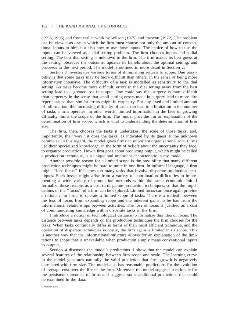
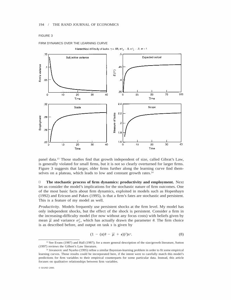
▫ Gibrat’s Law. The results for the model can also be compared to the literatureon the growth of firm size. Figure 3 depicts the learning curve and its impact on scope,scale, and expected output for the firm. Because of the gradual slowdown of learningthat results from the Bayes’ rule updating equation for s , the firm grows more quickly2

m

when it is young and small. This is consistent with much of the evidence from firm

11 This logic is equally applicable if x is a vector of inputs, so that each task is produced As f (x)g. Thederivation is an application of Euler’s Law for homogeneous functions.

12 The imposition of this sort of fixed costs is natural in equilibrium models of firm dynamics, since itforces a distinction between an exiting firm (which avoids paying F) and a firm that produces nothing butstays in the industry, and hence must pay F.


q RAND 2000.

FIGURE 3

FIRM DYNAMICS OVER THE LEARNING CURVE

panel data.13 Those studies find that growth independent of size, called Gibrat’s Law,is generally violated for small firms, but it is not so clearly overturned for larger firms.Figure 3 suggests that larger, older firms further along the learning curve find them-selves on a plateau, which leads to low and constant growth rates.14

▫ The stochastic process of firm dynamics: productivity and employment. Nextlet us consider the model’s implications for the stochastic nature of firm outcomes. Oneof the most basic facts about firm dynamics, exploited in models such as Hopenhayn(1992) and Ericson and Pakes (1995), is that a firm’s fates are stochastic and persistent.This is a feature of my model as well.

Productivity. Models frequently use persistent shocks at the firm level. My model hasonly independent shocks, but the effect of the shock is persistent. Consider a firm inthe increasing-difficulty model (for now without any focus costs) with beliefs given bymean m and variance s , which has actually drawn the parameter u. The firm choice2

m

is as described before, and output on task s is given by

(1 2 (s(u 2 m 1 e))2)xg. (8)

13 See Evans (1987) and Hall (1987); for a more general description of the size/growth literature, Sutton(1997) reviews the Gilbert’s Law literature.

14 Jovanovic and Nyarko (1995) refine a similar Bayesian-learning problem in order to fit some empiricallearning curves. Those results could be incorporated here, if the intent were to carefully match this model’spredictions for firm variables to their empirical counterparts for some particular data. Instead, this articlefocuses on qualitative relationships between firm variables.

MITCHELL / 195

q RAND 2000.

The formula for output (8) has a familiar interpretation: (1 2 (s(u 2 m 1 e))2) servesas a time-varying productivity term.

The firm’s productivity is serially correlated despite the independent shock e. Thefirm, observing u 1 e, updates its beliefs. The evolution of the mean of the beliefs, m,is now important. The new mean m 9 is given by (from Bayes’ rule)

m 9 5 lu 1 (1 2 l)m 1 le, (9)

where l 5 s /(s 1 s ). For a given u, serial correlation of m leads overall firm2 2 2m m e

productivity to be correlated.Here the model is in contrast to the typical assumptions about the process that are

assumed, for instance, in Hopenhayn (1992)–that the evolution of firm productivity isconstant over the firm’s lifetime. The correlation of m, and hence productivity, risesover time. Eventually s approaches zero and so (1 2 l) approaches one, meaning that2

m

the long-run correlation of productivity is one. This arises since m converges to u, sothat eventually the problem the firm faces is constant over time. At the beginning of afirm’s life, productivity is largely due to randomness (luck), since knowledge is rela-tively low. As the firm ages and accumulates knowledge, the effect of accumulatedknowledge makes the ‘‘luck’’ component relatively less important, and hence the cor-relation rises.

Another new implication of the learning model for the firm-productivity processis that it leads the variance of output of a given firm to be autocorrelated. In the casewhere g 5 .5, integration by parts yields a variance of productivity of

2 2 22 p 2(u 2 m ) 1 se2Var(Y) 5 s .e 2 2 31 2225 w (s 1 s )e m

Since m is autocorrelated, the variance of output is autocorrelated for each firm. In thelanguage of econometrics, output and productivity should show ARCH,15 despite theshocks being independent. Intuitively, firms with bad estimates of u, that is, firms thatdo not know very well how to operate their technology, have high variance of output.Those firms are likely to have bad estimates in the next period, and hence high variance,so the variance is autocorrelated.

Employment. When either the increasing-difficulty or the loss-of-focus models is usedto explain the limits to firm scope, expected productivity increases monotonically. Asa result, the model predicts that ‘‘older’’ is always synonymous with ‘‘bigger’’ (in termsof employment) and ‘‘more productive.’’ Although firms do tend to grow as they age,this monotonicity is inconsistent with data such as that presented by Hall (1987), whereemployment varies both up and down.

Unlike the model with only increasing difficulty of tasks, a model with both in-creasing difficulty and costs to loss of focus will allow the firm’s estimate of theunknown parameter, m, to influence not only realized productivity but expected pro-ductivity, and therefore affect employment decisions. Since m fluctuates randomly, thiswill give rise to randomness in employment. The Bayesian-learning structure will gen-erate predictions for first- and second-moment properties of employment dynamics thatcan be compared to the stylized facts of empirical studies on firm dynamics. This is a

15 Autoregressive conditional heteroskedasticity.


q RAND 2000.

real payoff of the Bayesian structure: since variances affect mean productivity, the first-and second-moment predictions are tied together. We can use the model to help un-derstand some of the key facts in such panel data studies as Evans (1987) and Hall(1987). Specifically, small firms grow faster than large firms on average, and smallfirms’ growth rates are more variable than those of large firms.

Consider the multiplicative form 1 2 (s(u 1 e) 2 qs)2, combined into a modelwith costs of focus, i.e., where f . 0. Again, for simplicity, suppose that xs must beconstant across all tasks, i.e., xs 5 x, for each production run. Tasks are progressivelymore difficult and cause a loss of focus. The firm chooses a set of tasks of the form[0, b]. As the firm incorporates more and more tasks, the tasks become increasinglydifficult. Simultaneously, the firm encounters loss of focus, since conditional on a givenexpectation of u, the firm is drawn to choose {qs} close to su in order to minimizelosses from the (s(u 1 e) 2 qs)2 term.

Variance in beliefs about u generates lower efficiency as before, since it leads qs

to be farther from su on average. In addition, however, the mean of beliefs m is alsoimportant. When u is larger in absolute value, the set of processes {qs} that minimizeslosses from the (s(u 1 e) 2 qs)2 term is steeper, and steeper profiles {qs} have a highercost resulting from loss of focus. Firms learning that they have drawn a large u (inabsolute value) will be forced to be smaller than firms that have drawn a smaller u. Asa result, firms adjust their scope and scale in response to changes in their estimate ofthe mean m of u as well as to the variance s , and so size is affected by the random2

m

fluctuations given in (9), which can go either up or down. At the same time, the factthat lower s allows the firm to choose {qs} more precisely will still tend to increase2

m

firm size.Once again, the quadratic form of the two loss functions from {qs} leads the firm

to choose a linear combination of the ‘‘no focus costs’’ optimal choice sm and theaverage technique q({qs}) defined earlier. Using the fact that the firm chooses an in-terval [0, b], the optimal profile can be characterized as follows.

Lemma 2. Suppose hs 5 1 2 (s(u 1 e) 2 qs)2. Then the optimal technique profile is

1 f bmq* 5 (sm ) 1 . (10)s 1 1 f (1 1 f) 2

Proof. A proof identical to Lemma 1, everywhere replacing s 1 m with sm, showsthat qs is of the form

1 fq 5 (sm ) 1 q ({q }).s s1 1 f 1 1 f

Since the firm chooses to produce over an interval [0, b], q can be calculated byintegrating qs:

1 fq 5 mb 1 q.

2(1 1 f) 1 1 f

Solving for q gives q 5 mb/2, and the result. Q.E.D.

To see the effect of m on the firm’s employment and output, consider the absolutedifference between sm and qs:

MITCHELL / 197

q RAND 2000.

f f bm f bzsm 2 q z 5 (sm ) 2 5 zm z s 2 .s ) ) ) )1 1 f (1 1 f) 2 1 1 f 2

This is increasing in zmz: whenever zmz is bigger, focus considerations cause the optimalprofile to be farther away from sm. On the other hand, consider the difference betweenqs and the average technique q:

mb 1 f bm 1 bq 2 5 (sm ) 2 5 zm z s 2 .s) ) ) ) ) )2 1 1 f (1 1 f) 2 1 1 f 2

Once again, this is increasing in zm z.Total output is

2 2 g(1 2 (s(u 1 e) 2 q ) 2 f(q 2 q ) ) f (x ) ds.E s s s sP

The effective productivity for each task, (1 2 (s(u 1 e) 2 qs)2 2 f(qs 2 q)2, isdecreasing in zm z, and therefore both xs and b are decreasing in zm z as well. As in theselection model, some firms draw a more favorable u than others. A larger draw of uindicates a less-productive technology, since the organizational structure qs needed tooperate varied tasks efficiently involves very disparate, and thus costly, productiontechniques.

Since m affects the firm’s scope and employment choices, all the stochastic resultsderiving from the nature of the evolution of m then pertain to both the scope of thefirm and employment at the firm. Since m is stochastic and varies in both directions,it is possible to explain stochastic employment moving both up and down, as in thedata. Scope is also stochastic: it can fall if the firm’s estimate of u rises in absolutevalue. Decreasing s causes the trend of both to be increasing through time, but the2

m

interrelation of hierarchical difficulty of tasks and focus considerations explains a sto-chastic process for both that is consistent with some of the key features of the data.

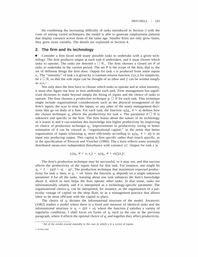
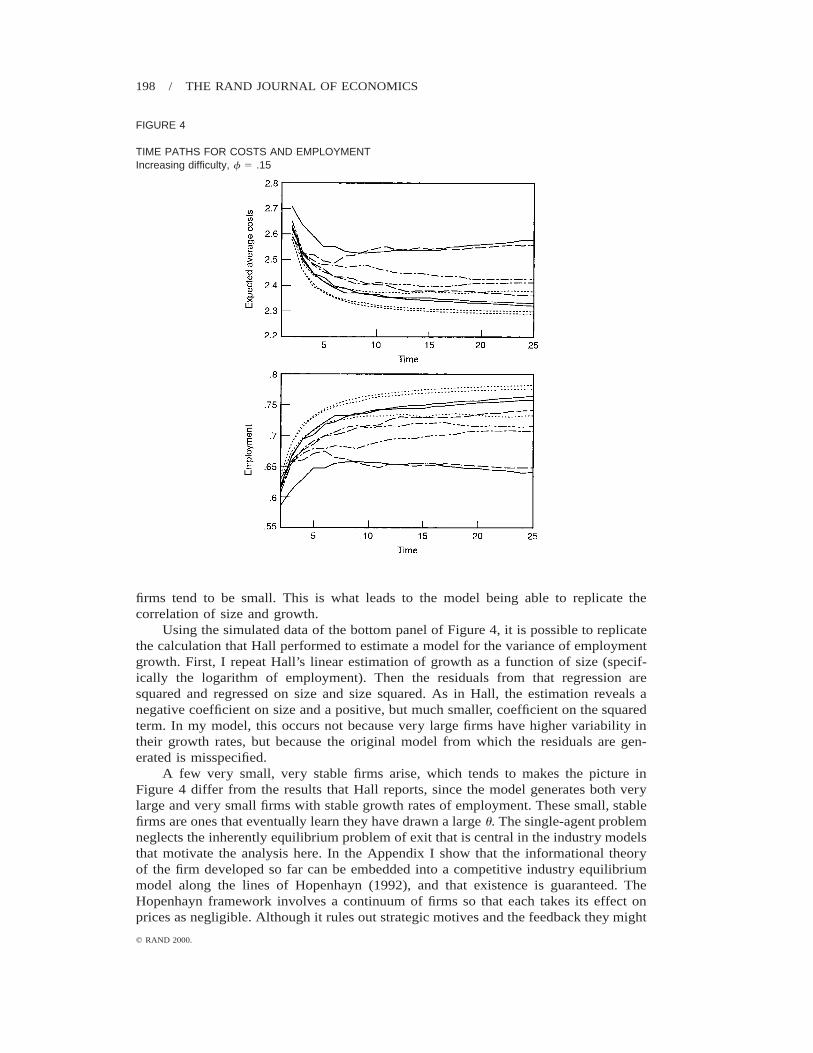
Since learning about u has two effects, one as a result of the monotonic decreasein variance and the other as a result of changes in the mean, I use simulations todemonstrate the implications of the model. Ten firms are simulated for 25 periods, andthe results are depicted in Figure 4. Parameters are the same as in Figure 3. The toppanel shows the paths of employment and expected average costs for the 25 periods.Firms tend to grow due to increased productivity, and with the imposition of a fixedcost (here set to one), average costs tend to fall. The bottom panel describes the samesimulated data, comparing growth rates of employment against the size (employment)of the firm.

As in Evans (1987) and Hall (1987), larger firms have smaller and less variablegrowth rates. As firms age, they learn about the u they have drawn. The lower variancehas the effect of increasing the size of firms because, as before, lower variance leadsto more accurate qs and higher efficiency. There are no predictable changes in m; somefirms learn that they have u that is large in absolute value, and they shrink; othersdiscover they have a small u and grow. Recall equation (9): the weight put on theshock e is s /(s 1 s ). This falls as s falls over the firm’s life, creating less variability2 2 2 2

m m e m

as the firm ages. Because firms tend to grow as s falls with age, the young, variable2m


q RAND 2000.

FIGURE 4

TIME PATHS FOR COSTS AND EMPLOYMENTIncreasing difficulty, f 5 .15

firms tend to be small. This is what leads to the model being able to replicate thecorrelation of size and growth.

Using the simulated data of the bottom panel of Figure 4, it is possible to replicatethe calculation that Hall performed to estimate a model for the variance of employmentgrowth. First, I repeat Hall’s linear estimation of growth as a function of size (specif-ically the logarithm of employment). Then the residuals from that regression aresquared and regressed on size and size squared. As in Hall, the estimation reveals anegative coefficient on size and a positive, but much smaller, coefficient on the squaredterm. In my model, this occurs not because very large firms have higher variability intheir growth rates, but because the original model from which the residuals are gen-erated is misspecified.

A few very small, very stable firms arise, which tends to makes the picture inFigure 4 differ from the results that Hall reports, since the model generates both verylarge and very small firms with stable growth rates of employment. These small, stablefirms are ones that eventually learn they have drawn a large u. The single-agent problemneglects the inherently equilibrium problem of exit that is central in the industry modelsthat motivate the analysis here. In the Appendix I show that the informational theoryof the firm developed so far can be embedded into a competitive industry equilibriummodel along the lines of Hopenhayn (1992), and that existence is guaranteed. TheHopenhayn framework involves a continuum of firms so that each takes its effect onprices as negligible. Although it rules out strategic motives and the feedback they might

MITCHELL / 199

q RAND 2000.

provide to the firm’s choice of scope, scale, and the learning problem, it supplies abaseline model for analyzing the interplay between firm dynamics and the organizationof production within an industry. Specifically, it allows for equilibrium exit by firmswith low productivity.

Equilibrium exit can reinforce the results on the model’s predictions for firm dy-namics. With a fixed cost F of operation, firms that discover they have a poor draw ofu exit, rather than developing into stable, small firms. Such firms, that is, firms withlarge zu z, must exit as their variance converges to zero whenever p is bounded and wis bounded away from zero.

Proposition 3. Suppose hs 5 1 2 (s(u 1 e) 2 qs)2, f . 0, there is a fixed cost F . 0any period the firm is in business, {pt} is bounded, and {wt} . c . 0 for all t. Thenthere exists a u* such that any firm with zu z . zu*z chooses to exit in the long run.

Proof. In the long run, the firm’s beliefs converge almost surely to zm z 5 u, s 5 0.2m

As u goes to infinity, scope b must go to zero, since the cost of implementing anyprofile {qs} that stays near the target su is prohibitively large. Since w is bounded awayfrom zero and p is bounded above, this implies that output goes to zero as zu z getslarge. A firm facing F . 0 and near-zero output forever will exit to avoid paying F.Q.E.D.

This sort of exit reinforces the result of Figure 4, since it removes small, stablefirms that arise as the long-run outcome of firms with high u.

5. Summary

n Evidence from panel data shows that firms vary widely both between one anotherand across time. A variety of industry equilibrium models have exploited this by as-suming that firm productivity follows some persistent stochastic process. The learningmechanism presented here, specifically a firm learning about an unknown parameter inits technology, can account for a variety of the facts associated with firm dynamics,and can be embedded in the sort of industry model that has been used to explain avariety of industry phenomena by using stochastic, persistent firm dynamics.

The model employs the concepts of the difficulty of tasks undertaken by the firmand the ‘‘focus’’ of a firm. The model can be used to derive implications for the natureof the firm. Here, the scope of the firm is limited by increasing difficulty of tasks andthe firm’s limited ability to focus on a wide variety of disparate production techniques.The informational structure yields an explanation for the limits to scope. The dynamicsof the learning process provide the means to compare the implications of the model tostudies of firm dynamics. The data to which it is well suited can be divided into threebroad categories.

First, the model explains some facts about the scope of firms. It explains why somuch diversification is into related fields, why larger firms tend to be more diversified,and why firms that are more diversified tend to be larger not only overall but also ateach activity they are involved with.

Second, the model can account for the learning curve, in the sense that averagecosts are nonincreasing over the lifetime of a firm, as many studies have found.

Third, the model can account for a variety of the stochastic properties that aresuggested by empirical studies of panel datasets of firms and their implications for firmsize, growth, and growth rate variability. Because the learning curve begins with fastgrowth and ends in a plateau, growth is negatively related to size for small firms, anempirical fact described by Sutton (1997). Despite the fact that all stochastic shocks


q RAND 2000.

are independent, the learning mechanism generates persistence in productivity and em-ployment, as evidenced in Evans (1987) and Hall (1987) and used in models of turnoversuch as Hopenhayn (1992). Older firms have less variable growth rates and tend to belarge. As a result, employment variability is negatively correlated with firm size, con-sistent with characteristics reported in Evans (1987) and Hall (1987). The model alsomakes predictions that have not been the focus of empirical research but may prove tobe fruitful avenues for future work. In particular, a variety of the firm variables areconditionally heteroskedastic, and the persistence of a firm’s outcome is increasing inthe age of the firm.

The model has implications for other applications that model learning. For in-stance, Foster and Rosenzweig (1995) use a Bayesian-learning model to study data onagricultural production in India. They look at the time following the ‘‘green revolu-tion,’’ which brought new agricultural methods to the farmers. They study the adoptiondecision of farmers who are uncertain about how to operate the new technology. Themodel presented here allows one to explore the farmer’s choice of the portfolio of cropshe grows, that is, the scope of agricultural production. The model predicts that scopewill move with scale as farmers learn. Farmers will start out operating a few of thenew-technology crops, then add to both the scale of those crops and the scope of cropsthey operate as they learn more about how to operate the new technology.

Several directions for further research are suggested by the shortcomings of themodel in this article. First of all, the model considers only the learning dynamics of afirm learning about a single technology. Since this is a single-parameter problem withcomplete learning, the model predicts that eventually learning slows to the point wherethe firm knows u perfectly and hence grows no further. Of course, firms are constantlyadopting and adapting to new technologies. Extending the model to include multiplepossible production technologies would allow, for instance, modelling the choice offirms to adopt new ideas. One could assess the role of information in the allocation ofnew ideas across firms. Specifically, one could compare what sort of new ideas areoperated by existing firms, which ones might have some transfer of knowledge fromthe process they have been operating, and when it is more likely that new, specializedfirms will undertake the new idea. Such a model is considered in Mitchell (1999).

Another area in which the model could be extended is in its equilibrium impli-cations. Only the simplest equilibrium model is considered here. One possible additionwould be to model each task as producing a good that entered separately into a con-sumer’s preferences. If only a few firms could efficiently produce the most difficultitems, output from that task would tend to have a high price. This sort of equilibriumconsideration would add to the picture of firm dynamics introduced here. In particular,it would extend the model of firm scope to demand-side effects, since the tastes ofconsumers across output from the various tasks would be an important determinant ofthe tasks an individual firm undertakes.

Finally, the model takes firms to be single-minded entities, when in fact firms, andthe knowledge produced along the learning curve, encompass a variety of people. Thesepeople must match, with each contributing his or her own knowledge to the firm. Someknowledge may be specific to the firm, and other knowledge may be applicable any-where. Using the informational approach to learning to build this sort of model of thefirm is another avenue for future research that would shed light on some importantissues in firm behavior.

Appendixn Existence of industry equilibrium. I describe a competitive industry model where the firms have thelearning technology described in the body of the article. Equilibrium is defined and existence is proven.

MITCHELL / 201

q RAND 2000.

Suppose there are a large number (a continuum) of firms operating the technology each period, witheither increasing difficulty, focus costs, or both. Entering firms draw a u from a normal distribution withmean u and variance s . Denote the measure defining this distribution by N0(u). The measure defining the2

0

shock e will be denoted by N(e). In order to define entry and exit, the model needs to have a fixed cost Fpaid by each firm for operating each period. This cost forces firms to decide between exiting and producingzero output. In addition, let there be a fixed cost E of entry. This avoids degeneracies where firms with baddraws instantly exit to be replaced by the free new draw of an entrant. Denote the measure induced by abelief m 5 (m, s ) ∈ R2 by Nm(u), i.e., it is generated by the open intervals of the form (2`, a):2

m

a 21 (u 2 m )N ((2`, a)) 5 exp 2 du.m E 21 22 2sÏ2ps m2` m

The firm’s static problem of maximizing profits, net of ‘‘focus’’ costs, given a belief m 5 (m, s ) ∈ R2,2m

a price p, and a wage w is

b b2(q 2 q )sgp(m, p, w) 5 max p f (x ) h (q , u 1 e) 2 f ds dN(e) dN (u) 2 w ·x ds 2 F.E E E s s s s m E s1 2l(P)x ,q ,bs s R R 0 0

Denote the solution to this problem by {x , q , b*}s∈[0,b]. From the body of the article, this is a well-defined* *s s

problem, it is clearly continuous, and it is bounded for any w . 0. Define the expected output,

b* 2(q* 2 q )sgy(m, p, w) 5 f (x*) h (q*, u 1 e) 2 f ds dN(e) dN (u).E E E s s s s m1 2l(P)R R 0

Let x(m, p, w) be the associated labor demand for the firm:

b

x(m, p, w) 5 x*(m, p, w) ds.E s0

Concavity (g , 1) and continuity imply that x is unique for each s, as well as continuous in m, p, and w.*sAs a result, y and x are continuous functions.

There is a single dynamically relevant action a ∈ {0, 1} for the firm each period, where 1 denotes thatthe firm continues and 0 denotes that it exits. An equilibrium is a Borel measure tt(m, a), on R2 3 {0, 1},that is, on the states and actions of the incumbent firms, and a mass Mt ∈ R of firms entering in period t.As in Jovanovic and Rosenthal (1988), the topology of weak convergence is used for the space of Borelmeasures on R2 3 {0, 1} that contains tt. Industry output is defined by16

Y(t , M ) 5 ay(m, p , w ) dt (m, a) 1 M y(m , p, w),t t E t t t t 02R 3{0,1}

since continuing firms (a 5 1) contribute y(m, p, w), entrants contribute y(m0, p, w), and exiting firmscontribute nothing. Likewise, industry factor demand is

X(t, M) 5 ax(m, p , w ) dt (m, a) 1 M x(m , p, w).E t t t t 02R 3{0,1}

There is a continuous, bounded, downward-sloping demand function D(Y) for the industry’s homogeneousoutput such that industry revenue Y ·D(Y) is bounded, as well as a continuous, bounded, upward-slopingcontinuous supply function W(X) with W(0) . 0. Define the Borel measure on the next period’s mean andvariance m9, which is described by equations (2) and (9) as h(m9 z m, u 1 e). For a firm in state m, the evolutionof beliefs is given by the distribution G defining the conditional Borel measure on R2:

16 Here I exploit the fact that Bayes’ rule is unbiased. Expected output for an individual agent withbeliefs m and action a is the same as the actual expected output for a cohort of such agents.


q RAND 2000.

G(· z m, a) 5 ah(· z m, u 1 e) dN(e) dN (u).E E m

R R

For the transition G, continuity will be in the sense of the cumulative distribution function associated withthe measure G, which might be denoted, as in Jovanovic and Rosenthal, G(m9, m, a). Across a large numberof firms,17 the distribution of states m of active firms evolves according to its expectation, by the law of largenumbers. The law of motion is given by the operator C:

C(·, t , M ) 5 G(· z m) dt (m, a) 1 M G(· z m ).t t E t t 02R 3{0,1}

The first term reflects the evolution of states for continuing firms, the latter that for entering firms. Note thatthis is continuous in tt and Mt. Finally, the dynamic program of an incumbent firm is given by

1V (m, t) 5 max a p(m, p(t ), w(t )) 1 V (m9, t) dG(m9 z m, a) .t t t E t111 21 1 r 2a {0,1}∈ R

The variable a reflects exit: a firm may choose at the beginning of any period to exit (a 5 0) and receivezero from then on. The value zero reflects the idea that an exiter who chooses to reenter does so withoutany of the experience gained in earlier incarnations, i.e., knowledge is lost at exit. The option value of beingoutside the industry is zero, since the free-entry condition ensures that entrant profits are nonpositive.

Equilibrium requires that the marginal entrant have nonpositive expected profits, that almost every firmoptimize on the exit decision (which, in this case, simply amounts to the fact that it exits if its beginning-of-periodvalue falls below zero), that supply equal demand, and that the distribution be generated by the law of motion C.The initial condition is a distribution on states t0(m), where it is assumed that all firms have identical variance anda mean that is normally distributed.

Definition A1. A sequence {tt, Mt, pt, wt} is an industry equilibrium if`t50

(i) Entry decisions are optimal:

# EV (m , t )t 0 t 55 E, if M . 0.t

(ii) Exit decisions are optimal:

(tt(m, a) : aVt(m, tt) , 0) 5 0.(iii) Markets clear:

pt 5 D(Y(tt, Mt)) wt 5 W(X(tt, Mt)).

(iv) Individual decisions and the aggregate distributions coincide:

tt11(·, a) 5 C(·, tt, Mt).

Theorem A1. There exists an industry equilibrium when either hs 5 1 2 (s(u 1 e) 2 qs)2 and f $ 0(hierarchical difficulty of tasks) or hs 5 1 2 (s 1 u 1 e 2 qs)2 and f . 0 (focus).

The game has been formulated as an anonymous sequential game: all the incumbents, as well as a poolof potential entrants, are players. Players produce only if they have paid F in every period since paying theentry cost E. One ‘‘state’’ is being in business or not, but that is a binary set and thus compactness and anycontinuity restrictions are trivial, so I ignore it. To verify existence using Jovanovic and Rosenthal’s (1988)proof of existence of equilibrium in anonymous sequential games, we need to confirm five things. The firstthree assumptions are straightforward to verify.

17 Here, in addition to the fact that Bayes’ rule is an accurate representation across a large number ofdraws, a continuum law of large numbers is used, as in Jovanovic and Rosenthal (1987).

MITCHELL / 203

q RAND 2000.

(i) The action space is compact. Since it is {0, 1}, it is.(ii) The updating rule G is continuous. This is immediate from continuity of the normal distribution, con-

tinuity in the updating rules for Bayes’ rule on normal distributions, and the fact that a lies in a discrete set.(iii) The single-period reward p(m, p(tt), w(tt)) is continuous in m and tt and bounded: this is true since

p is bounded above and w . 0 because W is increasing and W(0) . 0, and both are continuous in tt.

Two assumptions are less immediate:

(iv) The total mass of players can be bounded (Jovanovic and Rosenthal normalize the mass to one,for instance).

Claim A1. The mass of players can be bounded above.

Proof. Because of the assumption that industry revenue is bounded, the industry cannot profitably supportan infinite number of firms. Industrywide revenue is bounded by R in each period. If a mass of firms, callits measure St, are in operation, total industry profits from t on, denoted , are bounded above byp t

1p , R 2 (S ·F),tt 1 21 2 b

i.e., the maximum revenue R forever minus fixed costs for the S firms in operation. Since F . 0, there existssome S such that if S . S, then total industry profits are negative from t on. Since Bayes’ rule is an unbiasedestimator, V(m, t) dtt is the total profits that will be made by all firms in operation at t over the course of their#lives. But since entry is free, future entrants contribute nothing to industry profits, and so V(m, t) dtt 5 . For# pt

all St bigger than S, though, is negative, which implies that V(m, t) must be negative for some firmp t

operating at time t. Therefore it is impossible for St to ever exceed S, since V(m, t) , 0 contradicts that allfirms in operation can make at least zero from exiting. Q.E.D.

Finally,

(v) The state space is compact.

When we have either increasing difficulty or focus, but not both, m can be eliminated as a state variable.The variance of m is contained in [0, m0]. As a result, the state space of beliefs m for the agents is compact,and the proof is complete.

When both f . 0 and there is increasing difficulty, m is a state variable, and m is not bounded. Constructa pseudo-industry by bounding m by constants and eliminating from the industry all firms with beliefs6km

that end a period outside those bounds. Take a sequence {k } that approaches infinity as i grows large.im

Define the truncated equilibrium state-action distribution for incumbents by t and the mass of entrants byit

M . Consider the sequence of prices {pt, wt}i associated with the sequence of equilibrium for the truncatedit

economies. Since both the prices are bounded by assumption on D and S, the price sequence is an elementof a compact set (in the product topology), as is Mt, by the previous argument (Claim A1). Therefore, thereexists a convergent subsequence {pt, wt, Mt}n. Denote the state-action distributions on this subsequence t n.The remainder of the proof argues that the limit of these truncated equilibria constitutes an equilibrium, sincethe normal distribution puts almost no weight in the tails for large n. First, it is shown that t n does indeedconverge to some limit distribution t.

Claim A2. The limit of the truncated economies t n exists.

Proof. The proof has two steps: the actions converge because the prices converge, and the states convergebecause the actions and the Mt’s converge. Throughout, take A 5 As 3 Aa to be an arbitrary finite intersectionof open intervals in R2 3 {0, 1}. The set of all such sets is a convergence determining class (see Stokey,Lucas, and Prescott, 1989), and so convergence on an arbitrary set of that form is sufficient to show con-vergence. Starting with the given initial condition t0(m), iteratively construct the action distribution from thedistribution of states t byn

s

t (As, Aa) 5 t (m: m ∈ As and a(m, p ) ∈ Aa)n n nt s t

and construct the state distribution t (As, ·) according tont11

t (As, Aa) 5 C(As, t , M ).n n nt11 t t

Given a state distribution at time t and a sequence of prices pn, the distribution of actions t (As, Aa) convergesnt

since the decision rule a is continuous. Continuity of C guarantees that the state distribution t (As, t , M )n n nt11 t t

converges as t and M do. Q.E.D.n nt t


q RAND 2000.

The final step shows that the limiting distribution t is an equilibrium.

Claim A3. The limit of the truncated economies t n is an industry equilibrium.

Proof. For any Borel-subset E of R2 3 {0, 1}, define tt(E) 5 limn→` t (E) and let Mt 5 limn→` M . Continuityn nt t

of C directly implies that part (iv) of the definition of equilibrium is satisfied:

n nt (·, a) 5 C ·, lim t (E), lim M 5 C(·, t , M ).t11 t t t t1 2n→` n→`

Market clearing can be shown by asserting that the limit economy has pt 5 lim p and wt 5 lim wn nt t

and by verifying that this is an equilibrium. In that case, continuity of x and y and the fact that t convergesnt

weakly implies

n n n n n n nlim X(t , M ) 5 lim ax(m, p , w ) dt (m, a) 1 M x(m , p , w )t t E t t t t 0 t t2n→` n→` R 3{0,1}

5 ax(m, p , w ) dt (m, a) 1 M x(m , p , w ) 5 X(t , M )E t t t t 0 t t t t2R 3{0,1}

and

n n n n n n nlim Y(t , M ) 5 lim ay(m, p , w ) dt (m, a) 1 M y(m , p , w )t t E t t t t 0 t t2n→` n→` R 3{0,1}

5 ay(m, p , w ) dt (m, a) 1 M y(m , p , w ) 5 Y(t , M ),E t t t t 0 t t t t2R 3{0,1}

so Y(t , M ) → Y(tt, Mt) and X(t , M ) → X(tt, Mt). Consequently, p → D(Y(tt, Mt)) and w → W(X(tt, Mt)),n n n n n nt t t t t t

and hence markets clear for tt, Mt, pt 5 lim p , and wt 5 lim w .n nt t

Given pt 5 lim p and wt 5 lim w , continuity of the reward in the prices implies thatn nt t

Vt(m, tt) 5 lim V (m, t ). Continuity of V implies that parts (i) and (ii) are satisfied: if Mt . 0, then M . 0n n nt t t

for all sufficiently high n, and therefore V (m0, t ) 5 0 for all sufficiently high n, so Vt(m0, tt) 5 0; if Mt # 0,n nt t

then V (m0, t ) # 0 for all sufficiently high n, so Vt(m0, tt) # 0. Finally, if aVt(m, tt) 5 lim aV (m, t ) isn n n nt t t t

smaller than zero, then it must also be negative for all n sufficiently large, but (t (m, a):aV (m, tt) , 0) 5 0,n nt t

so therefore (tt(m, a): aVt(m, tt) , 0) 5 0.The limit t satisfies all of the conditions of the definition of an equilibrium. Q.E.D.

References

ARGOTE, L. AND EPPLE, D. ‘‘Learning Curves in Manufacturing.’’ Science, Vol. 247 (1990), pp. 920–924.AUERSWALD, P., KAUFFMAN, S., LOBO, J., AND SHELL, K. ‘‘The Production Recipe Approach to Modeling

Technological Innovations: An Application to Learning by Doing.’’ CAE Working Paper no. 98-10,Cornell University, 1998.

CARDINAL, L. AND OPLER, T. ‘‘Corporate Diversification and Innovative Efficiency: An Empirical Study.’’Journal of Accounting and Economics, Vol. 19 (1995), pp. 365–381.

ERICSON, R. AND PAKES, A. ‘‘Markov-Perfect Industry Dynamics: A Framework for Empirical Work.’’ Reviewof Economic Studies, Vol. 62 (1995), pp. 53–82.

EVANS, D. ‘‘Tests of Alternative Theories of Firm Growth.’’ Journal of Political Economy, Vol. 95 (1987),pp. 657–674.

FOSTER, A. AND ROSENZWEIG, M. ‘‘Learning by Doing and Learning from Others: Human Capital and Tech-nical Change in Agriculture.’’ Journal of Political Economy, Vol. 103 (1995), pp. 1176–1209.

GORT, M. Diversification and Integration in American Industry. Princeton: Princeton University Press, 1962.HALL, B. ‘‘The Relationship Between Firm Size and Firm Growth in the U.S. Manufacturing Sector.’’ Journal

of Industrial Economics Vol. 35 (1987), pp. 583–606.HOPENHAYN, H. ‘‘Entry, Exit, and Firm Dynamics in Long Run Equilibrium.’’ Econometrica, Vol. 60 (1992),

pp. 1127–1150.IRWIN, D. AND KLENOW, P. ‘‘Learning-by-Doing Spillovers in the Semiconductor Industry.’’ Journal of Po-

litical Economy, Vol. 102 (1994), pp. 1200–1227.JOVANOVIC, B. ‘‘Selection and the Evolution of Industry.’’ Econometrica, Vol. 50 (1982), pp. 649–670.

MITCHELL / 205

q RAND 2000.

AND MACDONALD, G. ‘‘The Life Cycle of a Competitive Industry.’’ Journal of Political Economy,Vol. 102 (1994), pp. 322–347.

AND NYARKO, Y. ‘‘A Bayesian Learning Model Fitted to a Variety of Empirical Learning Curves.’’Brookings Papers on Economic Activity, Microeconomics (1995), pp. 247–299.

AND . ‘‘Learning by Doing and the Choice of Technology.’’ Econometrica, Vol. 64 (1996),pp. 1299–1310.

AND . ‘‘Stepping Stone Mobility.’’ Carnegie-Rochester Conference Series on Public Policy,Vol. 46 (1997), pp. 289–325.

AND ROSENTHAL, R. ‘‘Anonymous Sequential Games.’’ Journal of Mathematical Economics, Vol. 17(1988), pp. 77–87.

LUCAS, R. ‘‘On the Size Distribution of Business Firms.’’ Bell Journal of Economics, Vol. 9 (1978), pp. 508–523.

MITCHELL, M. ‘‘Adoption and the Size Distribution of Establishments.’’ Mimeo, University of Minnesota,1999.

PRESCOTT, E. ‘‘The Multi-Period Control Problem Under Uncertainty.’’ Econometrica, Vol. 40 (1972), pp.1043–1058.

AND VISSCHER, M. ‘‘Organization Capital.’’ Journal of Political Economy, Vol. 88 (1980), pp. 446–461.

ROTEMBERG, J. AND SALONER, G. ‘‘Benefits of Narrow Business Strategies.’’ American Economic Review,Vol. 84 (1994), pp. 1330–1349.

SALTER, M.S. AND RAVENSCRAFT, D. Diversification Through Acquisition. New York: Free Press, 1979.SHAW, K. ‘‘Discussion of Jovanovic and Nyarko (1995).’’ Brookings Papers on Economic Activity, Micro-

economics (1995), pp. 300–302.STOKEY, N., LUCAS, R., AND PRESCOTT, E. Recursive Methods in Economic Dynamics. Cambridge, Mass.:

Harvard University Press, 1989.SUTTON, J. ‘‘Gibrat’s Legacy.’’ Journal of Economic Literature, Vol. 35 (1997), pp. 40–59.WILSON, D. ‘‘Informational Economies of Scale.’’ Bell Journal of Economics, Vol. 6 (1975), pp. 184–195.

The scope and organization of production: firm dynamics over the ...

Documents

Transcript of The scope and organization of production: firm dynamics over the ...