The Satellite – PBL Model Connection

• The microwave scatterometers, radiometers, SARs and altimeters have now provided nearly three decades of inferred surface winds over the oceans.

R. A. Brown 2005 EGU

• In many cases these products are revolutionary, changing the way we view the world.

SeaSat was launched in 1978as an oceanography satellite

* Primary mission was to determine ocean motion; geostrophic and surface layer.• Seasat had a scatterometer to measure surface small-scale roughness, inferring surface stress.

* The scatterometer data have been extensively studied and compared to in situ measurements — they comprise a ‘surface truth’ base of surface winds.

* Seasat also had a SAR to determine sea state, an altimeter to determine ocean height and a radiometer to determine attenuation of the signals.

1980 – 2005: Using surface roughness as a lower boundary condition on the PBL, considerable information about

the atmosphere and the PBL has been inferred.

• The symbiotic relation between surface backscatter data and the PBL model has been beneficial to both.

• The PBL model has established superior ‘surface truth’ winds (or pressures) for the satellite model functions.

• Satellite data have proven that the nonlinear PBL solution with OLE is observed most of the time.

Includes a rotating frame of reference

R. A. Brown 2003 U. ConcepciÓn

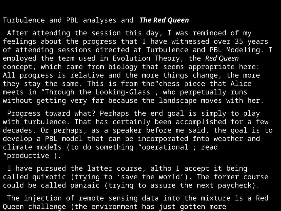
Turbulence and PBL analyses and The Red Queen

After attending the session this day, I was reminded of my feelings about the progress that I have witnessed over 35 years of attending sessions directed at Turbulence and PBL Modeling. I employed the term used in Evolution Theory, the Red Queen concept, which came from biology that seems appropriate here: All progress is relative and the more things change, the more they stay the same. This is from the chess piece that Alice meets in “Through the Looking-Glass”, who perpetually runs without getting very far because the landscape moves with her.

 Progress toward what? Perhaps the end goal is simply to play with turbulence. That has certainly been accomplished for a few decades. Or perhaps, as a speaker before me said, the goal is to develop a PBL model that can be incorporated into weather and climate models (to do something “operational”; read “productive”).

 I have pursued the latter course, altho I accept it being called quixotic (trying to ‘save the world’). The former course could be called panzaic (trying to assure the next paycheck).

 The injection of remote sensing data into the mixture is a Red Queen challenge (the environment has just gotten more complicated, with a large supply of new and different data). But it has also been a boon to the analytic, similarity models. This is the essence of my talk.

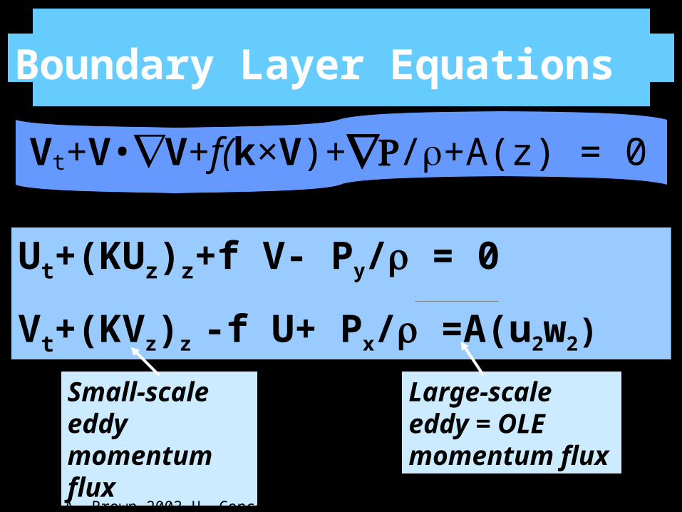
Ut+(KUz)z+f V- Py/ = 0

Vt+(KVz)z -f U+ Px/ =A(u2w2)

Vt+V•V+f(k×V)+/+A(z) = 0or

Small-scale eddy momentum flux

Large-scale eddy = OLE momentum flux

Boundary Layer Equations

R. A. Brown 2003 U. ConcepciÓn

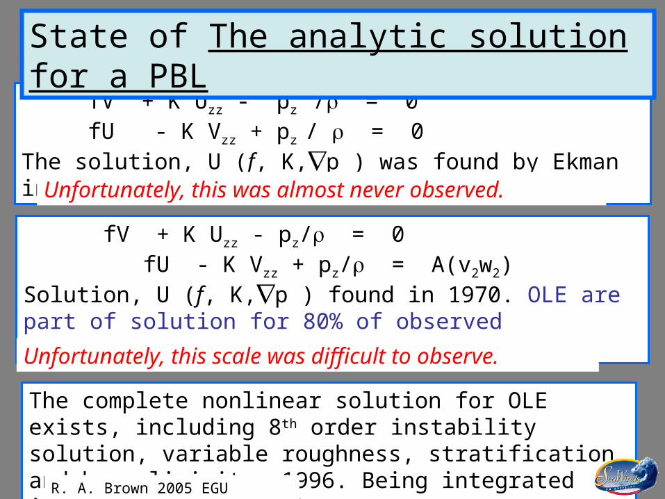
fV + K Uzz - pz / = 0 fU - K Vzz + pz / = 0The solution, U (f, K,p ) was found by Ekman in 1904.

State of The analytic solution for a PBL

fV + K Uzz - pz/ = 0 fU - K Vzz + pz/ = A(v2w2)Solution, U (f, K,p ) found in 1970. OLE are part of solution for 80% of observed conditions (near-neutral to convective).

Unfortunately, this was almost never observed.

The complete nonlinear solution for OLE exists, including 8th order instability solution, variable roughness, stratification and baroclinicity, 1996. Being integrated into MM5, NCEP (2005)

Unfortunately, this scale was difficult to observe.

R. A. Brown 2005 EGU

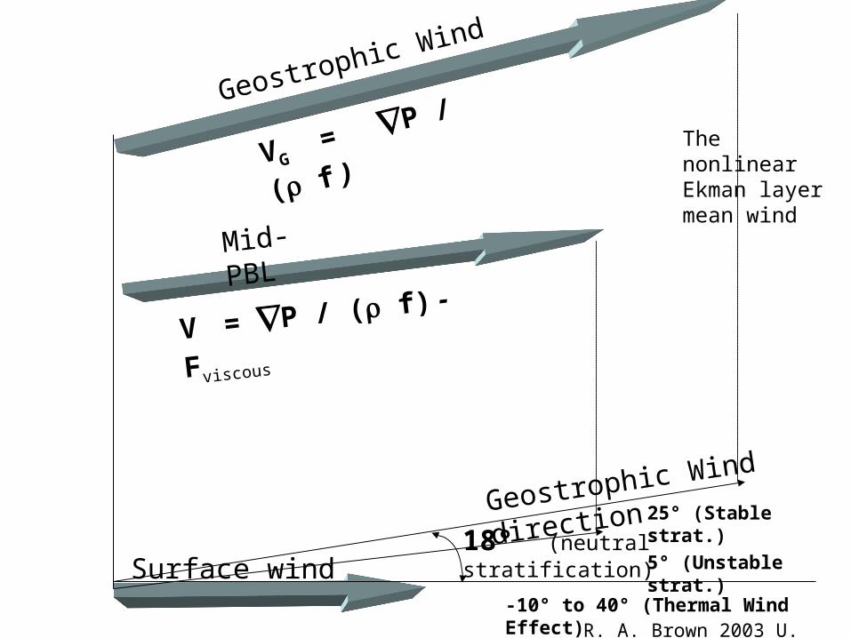
18° (neutral stratification)Surface wind

Geostrophic Wind direction

Geostrophic Wind

Mid- PBL

VG = P / ( f )

V = P / ( f) - Fviscous

25° (Stable strat.)

5° (Unstable strat.)

-10° to 40° (Thermal Wind Effect)R. A. Brown 2003 U. ConcepciÓn

The nonlinear Ekman layer mean wind

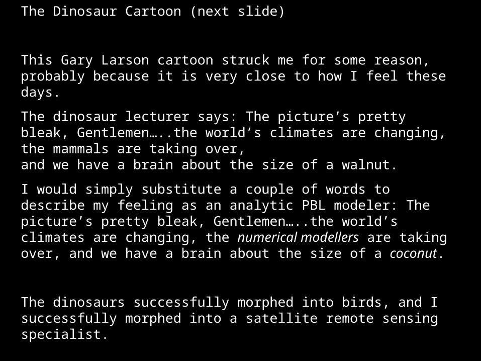
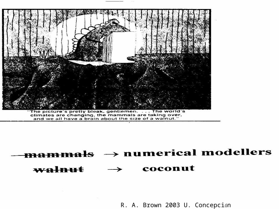
The Dinosaur Cartoon (next slide)

 

This Gary Larson cartoon struck me for some reason, probably because it is very close to how I feel these days.

The dinosaur lecturer says: The picture’s pretty bleak, Gentlemen…..the world’s climates are changing, the mammals are taking over, and we have a brain about the size of a walnut.

I would simply substitute a couple of words to describe my feeling as an analytic PBL modeler: The picture’s pretty bleak, Gentlemen…..the world’s climates are changing, the numerical modellers are taking over, and we have a brain about the size of a coconut.

 

The dinosaurs successfully morphed into birds, and I successfully morphed into a satellite remote sensing specialist.

R. A. Brown 2003 U. ConcepciÓn

Or, the mathematical solution for the PBL flow that includes coherent structures (Organized Large Eddies or OLE) is correct

R. A. Brown 2005 EGU

Status of organized large eddies (OLE) verification

• Airplane campaigns in cold air outbreaks (1976 - ).

• Ground based Lidar detects OLE (1996 -); Lidar from Aircraft PBL flights (1999 -).

• Satellite derived surface pressures (1997) using nonlinear PBL model are accurate.

• Satellite SAR data of ocean surface shows evidence of ubiquitous OLE (1978; 1986; 1997-).

R. A. Brown 2005 EGU

R.Foster 2003

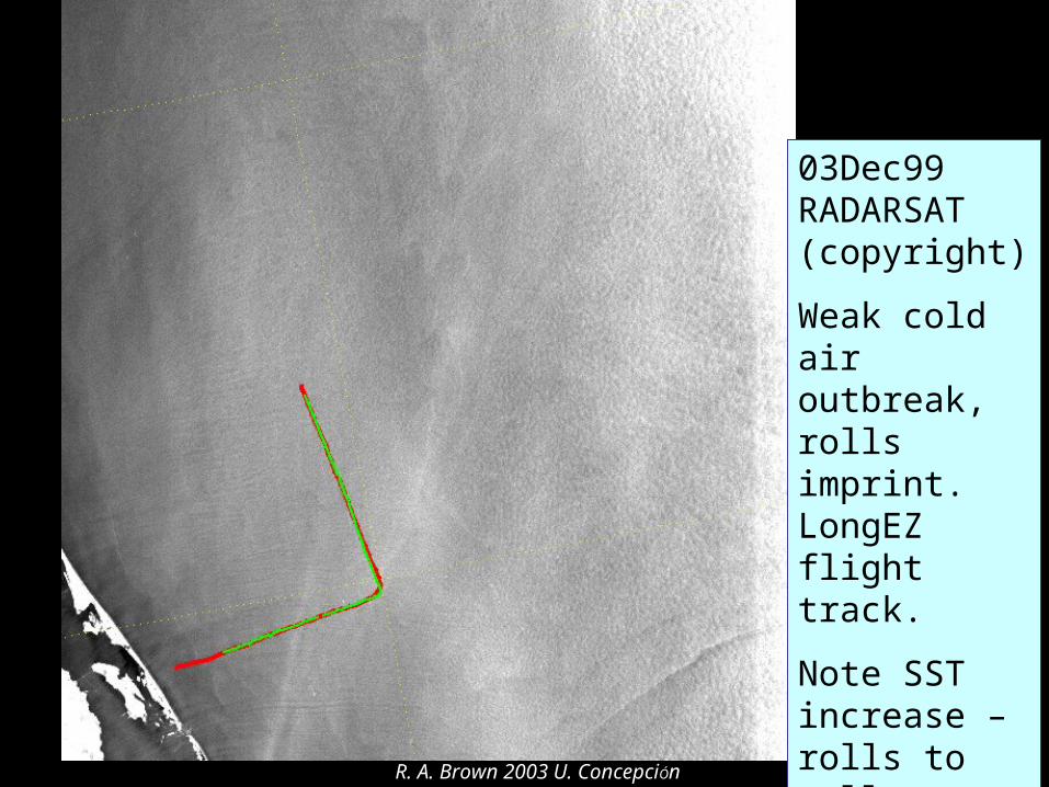
03Dec99 RADARSAT (copyright)

Weak cold air outbreak, rolls imprint. LongEZ flight track.

Note SST increase – rolls to cells; internal waves.

R. A. Brown 2003 U. ConcepciÓn

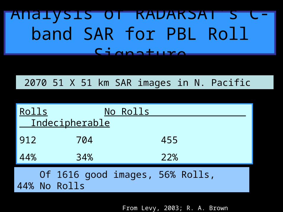
Analysis of RADARSAT’s C-band SAR for PBL Roll Signature

2070 51 X 51 km SAR images in N. Pacific

Rolls No Rolls Indecipherable

912 704 455

44% 34% 22%

Of 1616 good images, 56% Rolls, 44% No Rolls

From Levy, 2003; R. A. Brown 2005 EGU

Analysis of frequency of SAR PBL Roll Signature by

RADARSAT Of a random sampling of 7150 100 X 100 km SAR images of the North Pacific (1997 – 1999)

Minimum Occurrence of Roll Vortices by Month %

Jan Feb Mar Apr May --- Sep Oct Nov Dec

33 31 28 17 11 no 30 no 75 39 data data

Gad Levy, R.A. Brown 2001

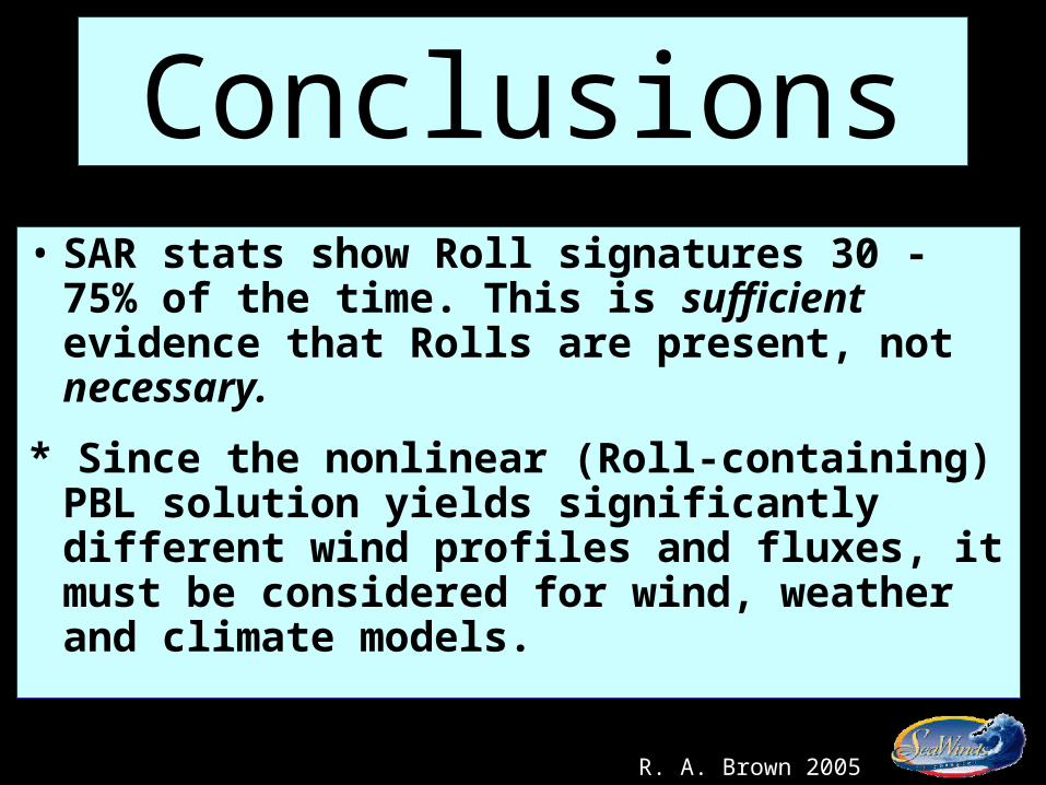
Conclusions• SAR stats show Roll signatures 30 - 75%

of the time. This is sufficient evidence that Rolls are present, not necessary.

* Since the nonlinear (Roll-containing) PBL solution yields significantly different wind profiles and fluxes, it must be considered for wind, weather and climate models.

R. A. Brown 2005 EGU

R. A. Brown 2004 EGU

The solution for the PBL boundary layer (Brown, 1974, Brown and Liu, 1982), may be written

U/VG = ei - e –z[e-iz + ieiz]sin + U2

where VG is the geostrophic wind vector, the angle between U10 and VG is [u*, HT, (Ta – Ts,)PBL] and the effect of the organized large eddies (OLE) in the PBL is represented by U2(u*, Ta – Ts, HT)

U/VG ={(u*), U2(u*), u*, zo(u*), VT(HT), (Ta – Ts), }

Or U/VG = [u*, VT(HT), (Ta – Ts), , k, a] = {u*, HT, Ta – Ts},

for = 0.15, k= 0.4 and a = 1

VG = (u*,HT, Ta – Ts) n(P, , f)

Hence P = n [u*(k, a, ), HT, Ta – Ts, , f ] fn(o)

This may be written:

In particular,

R. A. Brown 2003 U. ConcepciÓn

SLP from Surface Winds

• UW PBL similarity model joins two layers:

• Use “inverse” PBL model to estimate from satellite . Get non-divergent field UG

N.• Use Least-Square optimization to find best fit

SLP to swaths• There is extensive verification from ERS-1/2,

NSCAT, QuikSCAT

10 10( , , , , , )G

f P T SST q CSu

10

10logN

o

uU

k z u

10NU

P (UGN )

G

R. A. Brown 2005 EGU

Dashed:ECMWF R. A. Brown 2005 EGU

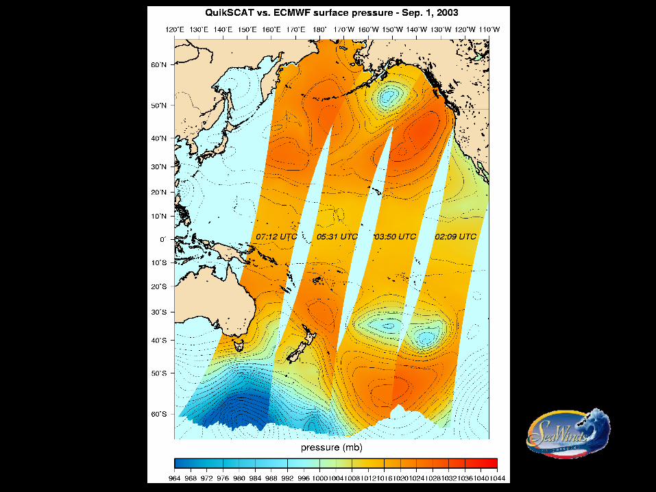
ECMWF analysis

QuikScat analysis

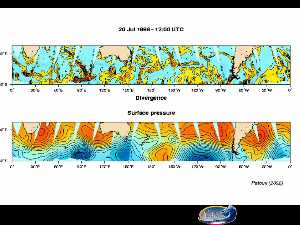
Surface Pressures

J. Patoux & R. A. Brown

Raw scatterometer windsUWPressure field smoothed

JPL Project Local GCM nudge smoothed = Dirth (with ECMWF fields)

(JPL)

R. A. Brown 2005 EGU

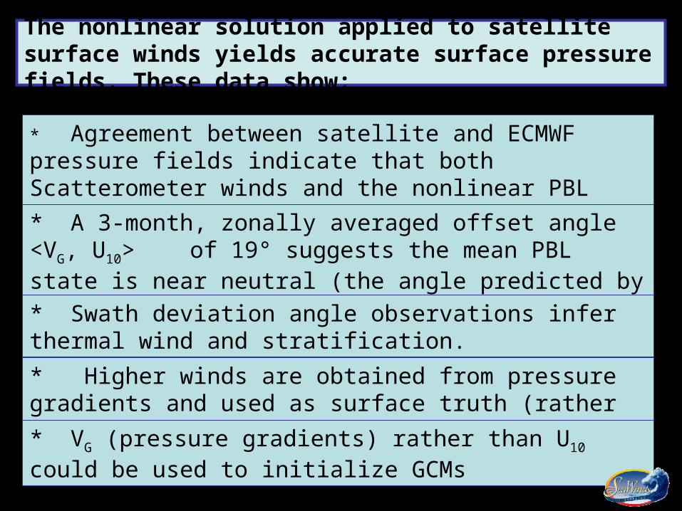
The nonlinear solution applied to satellite surface winds yields accurate surface pressure fields. These data show:

* Agreement between satellite and ECMWF pressure fields indicate that both Scatterometer winds and the nonlinear PBL model (VG/U10) are accurate within 2 m/s.

* A 3-month, zonally averaged offset angle <VG, U10> of 19° suggests the mean PBL state is near neutral (the angle predicted by the nonlinear PBL model).

* Swath deviation angle observations infer thermal wind and stratification.

* Higher winds are obtained from pressure gradients and used as surface truth (rather than from GCM or buoy winds).

* VG (pressure gradients) rather than U10 could be used to initialize GCMs

R. A. Brown 2005 EGU

R. A. Brown 2005 EGU

R. A. Brown, J. Patoux R. A. Brown 2005 EGU

These data allow study of the development of fronts in general and frontal waves in particular:

QuikScat reveals mesoscale features that are not captured by numerical models or other satellite-borne instruments, in particular the surface signature of frontal instabilities that sometimes develop into secondary cyclones (predictively?).

• See Jerome Patoux presentation

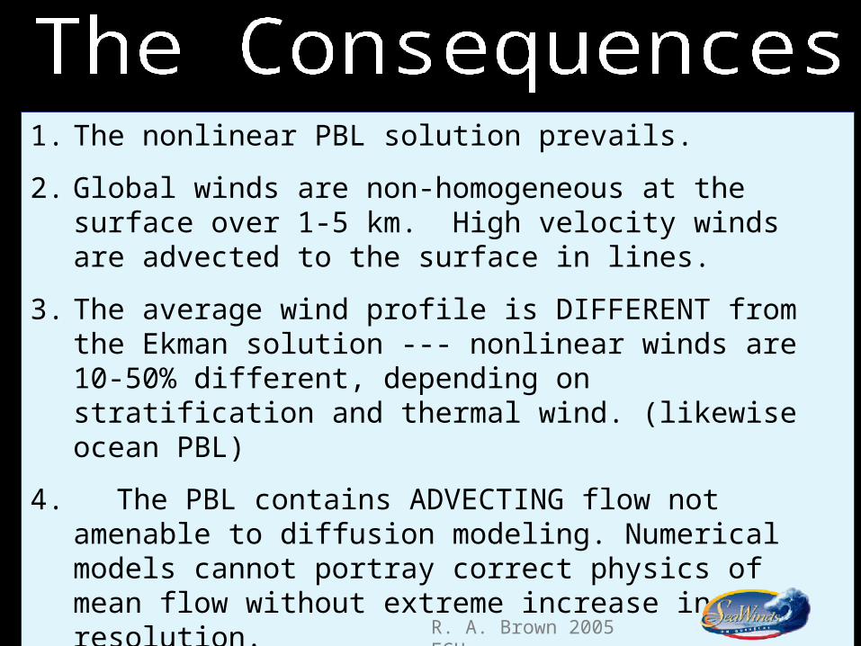
1. The nonlinear PBL solution prevails.

2. Global winds are non-homogeneous at the surface over 1-5 km. High velocity winds are advected to the surface in lines.

3. The average wind profile is DIFFERENT from the Ekman solution --- nonlinear winds are 10-50% different, depending on stratification and thermal wind. (likewise ocean PBL)

4. The PBL contains ADVECTING flow not amenable to diffusion modeling. Numerical models cannot portray correct physics of mean flow without extreme increase in resolution.

5. The correct PBL model allows excellent daily global satellite surface pressure analyses from space.

R. A. Brown 2005 EGU

Programs and Fields available onhttp://pbl.atmos.washington.edu

Questions to rabrown, neal or jerome@atmos.washington.edu

• Direct PBL model: PBL_LIB. (’75 -’00) An analytic solution for the PBL flow with rolls, U(z) = f( P, To , Ta , )

• The Inverse PBL model: Takes U10 field and calculates surface pressure field P (U10 , To , Ta , ) (1986 - 2000)

• Pressure fields directly from the PMF: P (o) along all swaths (exclude 0 - 5° lat.?) (2001) (dropped in favor of I-PBL)

• Global swath pressure fields for QuikScat swaths (with global I-PBL model) (2004)

• Surface stress fields from PBL_LIB corrected for stratification effects along all swaths (2005)

R. A. Brown 2005 EGU