The Sardinia Radio Telescope · The Sardinia Radio Telescope (SRT) is the new 64-m dish operated by...

Astronomy & Astrophysics manuscript no. AVpaperI.v4b c©ESO 2016January 11, 2016

The Sardinia Radio Telescope:

From a Technological Project to a Radio Observatory

I. Prandoni1,?, M. Murgia2, A. Tarchi2, and the AV team1, 2, 3

1 INAF-Istituto di Radioastronomia, Via P. Gobetti 101, I-40129 Bologna

2 INAF-Osservatorio Astronomico di Cagliari, Via della Scienza 5, I-09047 Selargius

3 INAF-Osservatorio Astronomico di Arcetri, Largo E. Fermi 5, I-50125 Firenze

Received ; accepted

ABSTRACT

Context. The Sardinia Radio Telescope (SRT) is the new 64-m dish operated by INAF (Italy). Its active surface, made of 1008separate aluminum panels supported by electromechanical actuators, will allow us to observe at frequencies up to 100 GHz. At themoment, three receivers, one per focal position, have been installed and tested: a 7-beam K-band receiver, a mono-feed C-bandreceiver and a coaxial dual-feed L-P band receiver. The SRT has been officially opened in October 2013, upon completion of itstechnical commissioning. The astronomical validation is proceeding in phases, following the implementation and/or fine-tuning ofadvanced sub-systems like e.g. the active surface, the derotator, new releases of the acquisition software, etc. Shared-risk/early-scienceobservations are being offered in steps, as soon as the relevant observing modes are validated.Aims. Highest priority was given to the validation of the SRT for observations as part of European networks. This activity can beconsidered concluded, and the SRT participates in shared risk mode to EVN and LEAP observing sessions since early 2014. The aimof this paper is to report on the astronomical validation of the SRT for single-dish operations.Methods. As part of the astronomical validation activities, different observing modes were tested and validated, and first astronomicalobservations were carried out to demonstrate the SRT science capabilities. In addition we developed astronomer-oriented SW tools.Results. This paper presents the first results of the astronomical validation activity of the SRT as a single dish, with particular focuson C-band performance with the commissioning backends. Single-dish performance at L- and K-bands are still ongoing and will bepresented in following papers. One of the main objectives of the AV is the identification of deficiencies in the instrumentation and/orin the telescope control software for further optimization. As a result of this, the overall telescope performance has been significantlyimproved.

Key words. Telescopes – Methods: observational

1. Introduction

The Sardinia Radio Telescope1 is a new general purpose, fully-steerable 64-m diameter parabolic radio telescope capable ofoperating with high efficiency in the 0.3-116 GHz frequencyrange. The instrument is the result of a scientific and technicalcollaboration among three Structures of the Italian National In-stitute for Astrophysics (INAF): the Institute of Radio Astron-omy of Bologna, the Cagliari Astronomy Observatory, and theArcetri Astrophysical Observatory in Florence. The main fund-ing agencies are the Italian Ministry of Education and ScientificResearch, the Sardinia Regional Government, the Italian SpaceAgency (ASI), and INAF itself.

The SRT is located in the plain of Pranu Sanguni, 35 kmnorth of Cagliari (IT), in the municipality of San Basilio. Themanufacturing of its mechanical parts and their assembly on-sitewas commissioned in 2003 and completed in mid 2012. The an-tenna was officially opened on September 30th 2013, upon com-pletion of the technical commissioning. The Astronomical Vali-dation (AV) is now well underway and early science/shared risk

? e-mail: [email protected] www.srt.inaf.it

observations are foreseen to start in 2016. The SRT is planned tobe used for astronomy, geodesy and space science, both as a sin-gle dish and as part of the European and International networks.

After the first successful VLBI (Very Long Baseline Interfer-ometry) data correlation, obtained between the SRT and Medic-ina stations in January 2014, the SRT regularly participated inEVN (European VLBI Network) test observations (Migoni et al.2014), and since 2015 the SRT is offered as an additional EVNstation in shared-risk mode for all of its three first-light observ-ing bands (L-, C- and K-bands). In addition, we have success-fully implemented the LEAP (Large European Array for Pulsars)project at SRT, having installed all of the hardware and softwarenecessary for the project (Perrodin et al. 2014). The SRT partic-ipates in monthly LEAP runs, for which data acquisition is nowfully automated. The use of the SRT in the context of Europeannetworks can therefore be considered completed, and we refer toPrandoni et al. (2014) for a more detailed discussion. The firstresults of LEAP operations are discussed in Bassa et al. (2016)and Perrodin et al. (2016).

The aim of this paper is to report on the astronomical vali-dation of the SRT for single-dish operations. The AV is carriedout in steps, from basic "on-sky" tests aimed at verifying the

Article number, page 1 of 17page.17

A&A proofs: manuscript no. AVpaperI.v4b

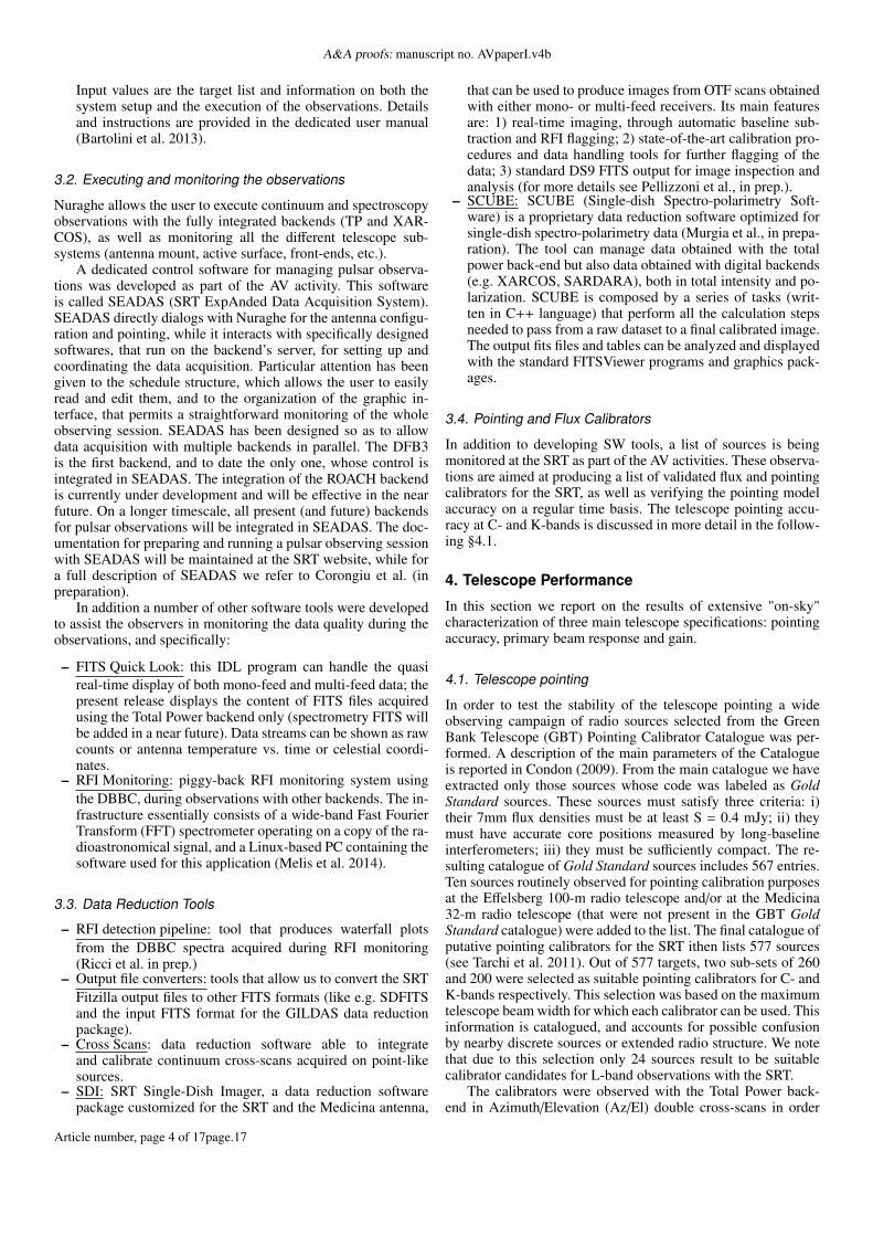
Table 1. The SRT technical specifications

Elevation range 5◦ − 90◦Azimuth range ±270◦Azimuth slewing speed 51◦/minElevation slewing speed 30◦/minSurface accuracy 305 µm @45◦ ElPointing accuracy(∗) 2/13 arcsec (@ 22 GHz)

(∗) Specs for normal conditions, with/without metrology implemented

general performance and/or the limits of the telescope and theacquisition systems, to more complex acquisitions aimed at as-sessing the actual SRT capabilities for typical scientific observa-tions. Examples of the former are: the verification of the backendlinearity range, the verification of the On-The-Fly (OTF) scanpointing accuracy and maximum exploitable speed, the mea-surement of the confusion noise, and an accurate characteriza-tion of the beam side-lobes. Examples of the latter are contin-uum and/or spectroscopic acquisitions, including mapping of ex-tended sources, pulsar timing, etc. This paper is the first of aseries reporting the results of the validation of SRT single-dishoperations.

2. The SRT in a nutshell

The SRT has a shaped Gregorian optical configuration with a 7.9m diameter secondary mirror and supplementary Beam-Wave-Guide (BWG) mirrors. With four possible focal positions (pri-mary, Gregorian, and two BWGs), the SRT will be able to allo-cate up to 20 remotely controllable receivers (Buttu et al. 2012).In its first light configuration the SRT is equipped with three re-ceivers, one per focal position: a 7-beam K-band (18-26 GHz)receiver (Gregorian focus), a mono-feed C-band receiver, cen-tered at the 6.7 GHz methanol line (Beam Wave Guide - BWG- focal position) and a coaxial dual-feed L-P band receiver (cen-tral frequencies 1.55 GHz and 350 MHz respectively, primaryfocus). One of the most advanced technical features of the SRTis the active surface: the primary mirror is composed by 1008panels supported by electromechanical actuators digitally con-trolled to compensate for deformations. Table 1 reports the maintechnical specifications of the telescope. We note that the sur-face accuracy reported in Table 1 refers to photogrammetry panelalignment, which is the current implementation of the active sur-face at the SRT, and corrects for gravitational deformations only.This accuracy is appropriate for getting high-efficiency perfor-mance up to operating frequencies <∼ 50 GHz (and therefore alsofor the receiver suite currently available). Metrology techniqueswill be needed to correct for thermal and wind pressure defor-mations, and get high efficiency performance up to the maxi-mum frequency for which the SRT is designed to operate (∼ 100GHz). The active surface can be used also to re-shape the pri-mary mirror from a Gregorian shaped to a parabolic profile. Thisis recommended to increase the field of view and the efficiencywhen using the receivers positioned at the primary focus. Table 2summarizes the main parameters of the three first-light receivers,namely the radio frequency band covered by the receiver (RF-Band), the maximum instantaneous bandwidth (BWmax), the re-ceiver temperature (TRx), the system temperature (Tsys), the gain(G), the width at half power (HPBW) of the main lobe of the

telescope beam2, the focal position (Primary, Gregorian, BWG)at which the receiver is mounted, together with its focal ratio( f /D). The suite of backends currently available at the SRT islisted below (for more details we refer to Melis et al. 2015b):

Total Power (TP): 14 voltage-to-frequency converters to digi-tize the detected signals. Different Intermediate Frequency(IF) inputs can be selected from three focal points. Thesystem can be adjusted to select different instantaneousbandwidths (up to a maximum of 2 GHz), and to modify theattenuation level.

XARCOS: narrowband spectro-polarimeter with 16 inputchannels. The nominal working band is 125-250 MHz. Theband actually exploitable is 140-220 MHz. The numberof channels provided for each double-polarization feedis 2048 × 4 (full Stokes). The instantaneous bandwidthranges between 0.488 and 62.5 MHz. This means that theachievable maximum spectral resolution is ∼ 238 Hz. Upto four tunable sub-bands can be simultaneously employedin conjunction with the mono-feed operating at C-band, aswell as with the central feed of the K-band receiver. In thelatter case only two sub-bands can be simultaneously set incase of observations in nodding mode.

Digital Base Band Converter (DBBC): digital platform basedon a flexible architecture, composed by four ADC boards,1 GHz bandwidth each and four Xilinx FPGA boards fordata-processing. The DBBC platform is designed mainlyfor VLBI experiments. However, a different firmwareallowing wide-band spectrometry has been developed fordifferent purposes, like e.g. monitoring of Radio FrequencyInterferences (RFI, see § 3).

Digital Filter Bank Mark 3 (DFB3): FX correlator developedby the Australia Telescope National Facility, allowingfull-Stokes observations. It has four inputs with 1024 MHzmaximum bandwidth each and 8-bit sampling for highdynamic range. The DFB3 is suitable for precise pulsartiming and search, spectral line and continuum observationswith high time resolution. It allows up to 8192 spectralchannels, to counter the effects of interstellar dispersionwhen it is operated in pulsar mode, and for power spectrummeasurements in spectrometer mode.

ROACH: digital board developed by CASPER3. The center-piece of the board is a Xilink Virtex 5 FPGA. Currentlyit is configured with a personality providing 32 complexchannels of 16 MHz each (total bandwidth 512 MHz). Thisis the backend adopted for pulsar observations in the contextof LEAP.

SARDARA: The SArdinia Roach2-based Digital Architecturefor Radio Astronomy (SARDARA) is a new wide-bandmulti-feed digital backend currently under development; itwill be exploitable both for continuum studies and as full-Stokes spectrometer. The FPGA-based ROACH2 boards are

2 HPBW (in arcmin) roughly scales as k/ν, where k is a RF-band de-pendent constant and ν is the frequency (in GHz): k = 19.590 for P-band; k = 19.373 for L-band; 18.937 for C-band; k = 18.264 for K-band.3 Collaboration for Astronomy Signal Processing and Electronics Re-search.


I. Prandoni , M. Murgia , A. Tarchi , and the AV team: The Sardinia Radio Telescope:

Table 2. Reference values for relevant parameters of the SRT first-light receivers. Updated values are constantly reported on the SRT website.

Receiver RF Band BWmax TRx T ∗sys G HPBW† Focal position &(GHz) (MHz) (K) (K) (K/Jy) arcmin focal ratio (f/D)

L/P-band# 0.305-0.41 (P) 105 20 52 0.53 56.2 Primary: f/D=0.331.3-1.8 (L) 500 11 20 0.52` 12.6

C-band 5.7-7.7 2000 7.7 29 0.60 2.8 BWG: f/D=1.37

K band> 18-26.5 2000 22 75-80‡ 0.65⊥ 0.83 Gregorian: f/D=2.35

∗ System temperature measured at 45◦ elevation† Value at the central frequency of the RF band# Dual band coaxial receiver` Measurement performed with the primary mirror re-shaped to a parabolic profile> 7-element multi-feed receiver‡ Indicative values obtained in various 2 GHz sub-bands, at atmospheric opacity τ ∼ 0.04 − 0.06⊥ Average value in the elevation range 50◦ ÷ 80◦

used as main processing cores, together with an infrastruc-ture including GPU-based nodes, a 10 Gbe SFP+ switch anda powerful storage computer (Melis et al., in preparation). Apreliminary version of SARDARA, suitable only for single-feed double-polarization receivers, is already offered at thetelescope (see the SRT website for more information on thecurrently supported configurations).

Both TP and XARCOS are designed to exploit the multi-feed receiver operating at K-band (7 feeds ×2 polarizations, i.e.14 output channels), but can also be used for observations at C-band. The current Local Oscillator setup does not allow us touse XARCOS at P- and L-bands. The use of the Total Poweranalog backend, while in principle allowed, is not recommendedat P- and L-bands due to severe RFI pollution, that limits itsperformance (the RFI environment at the SRT site is extensivelydiscussed in Bolli et al. 2015). In the following we will thereforefocus on C- and K-band operations. The astronomical validationat K-band is limited here to basic tests with the central feed. Afull discussion of the multi-feed performance will be the focusof a following paper.

The telescope is managed by means of a dedicated controlsystem called Nuraghe (Orlati et al. 2012), developed within theDISCOS project (Orlati et al. 2015), aimed at providing all theItalian radio telescopes with an almost identical common con-trol system. Nuraghe is a distributed system developed using theALMA Common Software (ACS) framework. It handles all ofthe operations of the telescope, taking care of the mount and mi-nor servo motions, of the frontend setup and of the data acquisi-tion performed with the integrated backends - at present, the TPand XARCOS - producing standard FITS output files. Furtherback-ends can be exploited in semi-integrated or external modes.The user interface allows the real-time monitoring of all the tele-scope devices. Automatic procedures let the user easily carry outessential operations like focusing, pointing calibration, skydipscanning. Nuraghe supports observing modes such as siderealtracking, On-Off, On-The-Fly (OTF) cross-scans and mappingin the equatorial, galactic and horizontal coordinate frames. Fordetails and instructions we refer to the official documentation,available at the DISCOS project website4.

4 http://discos.readthedocs.org

For a full description of the SRT telescope we refer to theSRT technical commissioning paper (Bolli et al. 2015).

3. The SRT as an astronomical observatory

The AV included a preparatory phase, carried out during thetechnical commissioning of the telescope, when several externalsoftware tools were developed, in order to assist in the prepara-tion, execution and monitoring of the observations, as long as inthe data inspection and reduction. Some of such tools are (or arebeing) made publicly available, others are meant to support theobservatory personnel. In the following we give a brief descrip-tion of the main tools developed. For details and updates on thereleased versions of these tools we refer to the SRT website.

3.1. Preparing the observations

– ETC: The Exposure Time Calculator provides an estimate ofthe exposure time needed to reach a given sensitivity (or viceversa) under a set of assumptions on the telescope setup andthe observing conditions. In its current version it includesboth the SRT and Medicina telescopes. Details and instruc-tions are provided in the dedicated user manual (Zanichelliet al. 2015).

– CASTIA: this software package provides radio source visi-bility information at user-selected dates for any of the threeItalian radio telescope sites (SRT, Medicina and Noto), aswell as for a collection of more than 30 international radiofacilities. The tool produces plots showing the visibility (andthe elevation) of radio-sources versus time, highlighting therise, transit and set times. Visual warnings are provided whenthe Azimuth rate is beyond the recommended limit and whensuperposition with the Sun and/or the Moon occurs. For adetailed description of the tool and of its usage we refer toVacca et al. (2013).

– Meteo Forecasting: this tool uses a numerical weather pre-diction model on timescales of 12/24 hours, to allow dy-namic scheduling (Nasyr et al. 2013).

– ScheduleCreator: this tool produces properly formattedschedules for Nuraghe, for all the available observing modes(sidereal, OTF scan and mapping, raster scan and mapping).



Input values are the target list and information on both thesystem setup and the execution of the observations. Detailsand instructions are provided in the dedicated user manual(Bartolini et al. 2013).

3.2. Executing and monitoring the observations

Nuraghe allows the user to execute continuum and spectroscopyobservations with the fully integrated backends (TP and XAR-COS), as well as monitoring all the different telescope sub-systems (antenna mount, active surface, front-ends, etc.).

A dedicated control software for managing pulsar observa-tions was developed as part of the AV activity. This softwareis called SEADAS (SRT ExpAnded Data Acquisition System).SEADAS directly dialogs with Nuraghe for the antenna configu-ration and pointing, while it interacts with specifically designedsoftwares, that run on the backend’s server, for setting up andcoordinating the data acquisition. Particular attention has beengiven to the schedule structure, which allows the user to easilyread and edit them, and to the organization of the graphic in-terface, that permits a straightforward monitoring of the wholeobserving session. SEADAS has been designed so as to allowdata acquisition with multiple backends in parallel. The DFB3is the first backend, and to date the only one, whose control isintegrated in SEADAS. The integration of the ROACH backendis currently under development and will be effective in the nearfuture. On a longer timescale, all present (and future) backendsfor pulsar observations will be integrated in SEADAS. The doc-umentation for preparing and running a pulsar observing sessionwith SEADAS will be maintained at the SRT website, while fora full description of SEADAS we refer to Corongiu et al. (inpreparation).

In addition a number of other software tools were developedto assist the observers in monitoring the data quality during theobservations, and specifically:

– FITS Quick Look: this IDL program can handle the quasireal-time display of both mono-feed and multi-feed data; thepresent release displays the content of FITS files acquiredusing the Total Power backend only (spectrometry FITS willbe added in a near future). Data streams can be shown as rawcounts or antenna temperature vs. time or celestial coordi-nates.

– RFI Monitoring: piggy-back RFI monitoring system usingthe DBBC, during observations with other backends. The in-frastructure essentially consists of a wide-band Fast FourierTransform (FFT) spectrometer operating on a copy of the ra-dioastronomical signal, and a Linux-based PC containing thesoftware used for this application (Melis et al. 2014).

3.3. Data Reduction Tools

– RFI detection pipeline: tool that produces waterfall plotsfrom the DBBC spectra acquired during RFI monitoring(Ricci et al. in prep.)

– Output file converters: tools that allow us to convert the SRTFitzilla output files to other FITS formats (like e.g. SDFITSand the input FITS format for the GILDAS data reductionpackage).

– Cross Scans: data reduction software able to integrateand calibrate continuum cross-scans acquired on point-likesources.

– SDI: SRT Single-Dish Imager, a data reduction softwarepackage customized for the SRT and the Medicina antenna,

that can be used to produce images from OTF scans obtainedwith either mono- or multi-feed receivers. Its main featuresare: 1) real-time imaging, through automatic baseline sub-traction and RFI flagging; 2) state-of-the-art calibration pro-cedures and data handling tools for further flagging of thedata; 3) standard DS9 FITS output for image inspection andanalysis (for more details see Pellizzoni et al., in prep.).

– SCUBE: SCUBE (Single-dish Spectro-polarimetry Soft-ware) is a proprietary data reduction software optimized forsingle-dish spectro-polarimetry data (Murgia et al., in prepa-ration). The tool can manage data obtained with the totalpower back-end but also data obtained with digital backends(e.g. XARCOS, SARDARA), both in total intensity and po-larization. SCUBE is composed by a series of tasks (writ-ten in C++ language) that perform all the calculation stepsneeded to pass from a raw dataset to a final calibrated image.The output fits files and tables can be analyzed and displayedwith the standard FITSViewer programs and graphics pack-ages.

3.4. Pointing and Flux Calibrators

In addition to developing SW tools, a list of sources is beingmonitored at the SRT as part of the AV activities. These observa-tions are aimed at producing a list of validated flux and pointingcalibrators for the SRT, as well as verifying the pointing modelaccuracy on a regular time basis. The telescope pointing accu-racy at C- and K-bands is discussed in more detail in the follow-ing §4.1.

4. Telescope Performance

In this section we report on the results of extensive "on-sky"characterization of three main telescope specifications: pointingaccuracy, primary beam response and gain.

4.1. Telescope pointing

In order to test the stability of the telescope pointing a wideobserving campaign of radio sources selected from the GreenBank Telescope (GBT) Pointing Calibrator Catalogue was per-formed. A description of the main parameters of the Catalogueis reported in Condon (2009). From the main catalogue we haveextracted only those sources whose code was labeled as GoldStandard sources. These sources must satisfy three criteria: i)their 7mm flux densities must be at least S = 0.4 mJy; ii) theymust have accurate core positions measured by long-baselineinterferometers; iii) they must be sufficiently compact. The re-sulting catalogue of Gold Standard sources includes 567 entries.Ten sources routinely observed for pointing calibration purposesat the Effelsberg 100-m radio telescope and/or at the Medicina32-m radio telescope (that were not present in the GBT GoldStandard catalogue) were added to the list. The final catalogue ofputative pointing calibrators for the SRT ithen lists 577 sources(see Tarchi et al. 2011). Out of 577 targets, two sub-sets of 260and 200 were selected as suitable pointing calibrators for C- andK-bands respectively. This selection was based on the maximumtelescope beam width for which each calibrator can be used. Thisinformation is catalogued, and accounts for possible confusionby nearby discrete sources or extended radio structure. We notethat due to this selection only 24 sources result to be suitablecalibrator candidates for L-band observations with the SRT.

The calibrators were observed with the Total Power back-end in Azimuth/Elevation (Az/El) double cross-scans in order



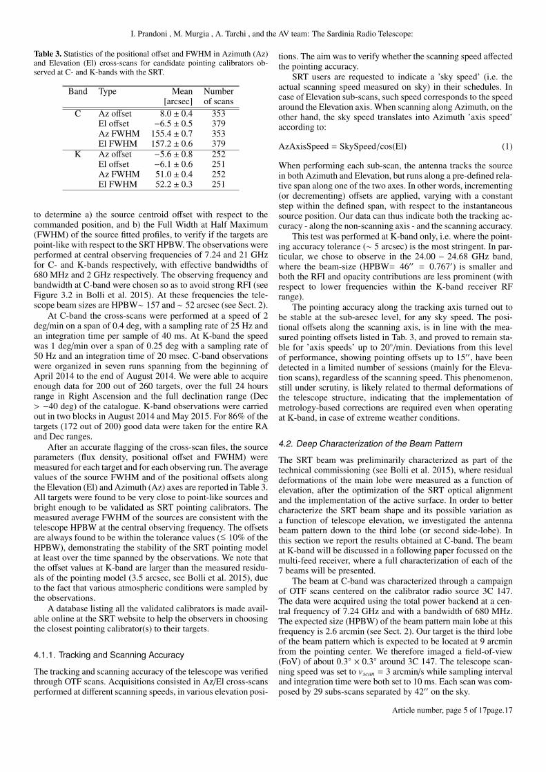
Table 3. Statistics of the positional offset and FWHM in Azimuth (Az)and Elevation (El) cross-scans for candidate pointing calibrators ob-served at C- and K-bands with the SRT.

Band Type Mean Number[arcsec] of scans

C Az offset 8.0 ± 0.4 353El offset −6.5 ± 0.5 379Az FWHM 155.4 ± 0.7 353El FWHM 157.2 ± 0.6 379

K Az offset −5.6 ± 0.8 252El offset −6.1 ± 0.6 251Az FWHM 51.0 ± 0.4 252El FWHM 52.2 ± 0.3 251

to determine a) the source centroid offset with respect to thecommanded position, and b) the Full Width at Half Maximum(FWHM) of the source fitted profiles, to verify if the targets arepoint-like with respect to the SRT HPBW. The observations wereperformed at central observing frequencies of 7.24 and 21 GHzfor C- and K-bands respectively, with effective bandwidths of680 MHz and 2 GHz respectively. The observing frequency andbandwidth at C-band were chosen so as to avoid strong RFI (seeFigure 3.2 in Bolli et al. 2015). At these frequencies the tele-scope beam sizes are HPBW∼ 157 and ∼ 52 arcsec (see Sect. 2).

At C-band the cross-scans were performed at a speed of 2deg/min on a span of 0.4 deg, with a sampling rate of 25 Hz andan integration time per sample of 40 ms. At K-band the speedwas 1 deg/min over a span of 0.25 deg with a sampling rate of50 Hz and an integration time of 20 msec. C-band observationswere organized in seven runs spanning from the beginning ofApril 2014 to the end of August 2014. We were able to acquireenough data for 200 out of 260 targets, over the full 24 hoursrange in Right Ascension and the full declination range (Dec> −40 deg) of the catalogue. K-band observations were carriedout in two blocks in August 2014 and May 2015. For 86% of thetargets (172 out of 200) good data were taken for the entire RAand Dec ranges.

After an accurate flagging of the cross-scan files, the sourceparameters (flux density, positional offset and FWHM) weremeasured for each target and for each observing run. The averagevalues of the source FWHM and of the positional offsets alongthe Elevation (El) and Azimuth (Az) axes are reported in Table 3.All targets were found to be very close to point-like sources andbright enough to be validated as SRT pointing calibrators. Themeasured average FWHM of the sources are consistent with thetelescope HPBW at the central observing frequency. The offsetsare always found to be within the tolerance values (<∼ 10% of theHPBW), demonstrating the stability of the SRT pointing modelat least over the time spanned by the observations. We note thatthe offset values at K-band are larger than the measured residu-als of the pointing model (3.5 arcsec, see Bolli et al. 2015), dueto the fact that various atmospheric conditions were sampled bythe observations.

A database listing all the validated calibrators is made avail-able online at the SRT website to help the observers in choosingthe closest pointing calibrator(s) to their targets.

4.1.1. Tracking and Scanning Accuracy

The tracking and scanning accuracy of the telescope was verifiedthrough OTF scans. Acquisitions consisted in Az/El cross-scansperformed at different scanning speeds, in various elevation posi-

tions. The aim was to verify whether the scanning speed affectedthe pointing accuracy.

SRT users are requested to indicate a ’sky speed’ (i.e. theactual scanning speed measured on sky) in their schedules. Incase of Elevation sub-scans, such speed corresponds to the speedaround the Elevation axis. When scanning along Azimuth, on theother hand, the sky speed translates into Azimuth ’axis speed’according to:

AzAxisSpeed = SkySpeed/cos(El) (1)

When performing each sub-scan, the antenna tracks the sourcein both Azimuth and Elevation, but runs along a pre-defined rela-tive span along one of the two axes. In other words, incrementing(or decrementing) offsets are applied, varying with a constantstep within the defined span, with respect to the instantaneoussource position. Our data can thus indicate both the tracking ac-curacy - along the non-scanning axis - and the scanning accuracy.

This test was performed at K-band only, i.e. where the point-ing accuracy tolerance (∼ 5 arcsec) is the most stringent. In par-ticular, we chose to observe in the 24.00 − 24.68 GHz band,where the beam-size (HPBW= 46′′ = 0.767′) is smaller andboth the RFI and opacity contributions are less prominent (withrespect to lower frequencies within the K-band receiver RFrange).

The pointing accuracy along the tracking axis turned out tobe stable at the sub-arcsec level, for any sky speed. The posi-tional offsets along the scanning axis, is in line with the mea-sured pointing offsets listed in Tab. 3, and proved to remain sta-ble for ’axis speeds’ up to 20◦/min. Deviations from this levelof performance, showing pointing offsets up to 15′′, have beendetected in a limited number of sessions (mainly for the Eleva-tion scans), regardless of the scanning speed. This phenomenon,still under scrutiny, is likely related to thermal deformations ofthe telescope structure, indicating that the implementation ofmetrology-based corrections are required even when operatingat K-band, in case of extreme weather conditions.

4.2. Deep Characterization of the Beam Pattern

The SRT beam was preliminarily characterized as part of thetechnical commissioning (see Bolli et al. 2015), where residualdeformations of the main lobe were measured as a function ofelevation, after the optimization of the SRT optical alignmentand the implementation of the active surface. In order to bettercharacterize the SRT beam shape and its possible variation asa function of telescope elevation, we investigated the antennabeam pattern down to the third lobe (or second side-lobe). Inthis section we report the results obtained at C-band. The beamat K-band will be discussed in a following paper focussed on themulti-feed receiver, where a full characterization of each of the7 beams will be presented.

The beam at C-band was characterized through a campaignof OTF scans centered on the calibrator radio source 3C 147.The data were acquired using the total power backend at a cen-tral frequency of 7.24 GHz and with a bandwidth of 680 MHz.The expected size (HPBW) of the beam pattern main lobe at thisfrequency is 2.6 arcmin (see Sect. 2). Our target is the third lobeof the beam pattern which is expected to be located at 9 arcminfrom the pointing center. We therefore imaged a field-of-view(FoV) of about 0.3◦ × 0.3◦ around 3C 147. The telescope scan-ning speed was set to vscan = 3 arcmin/s while sampling intervaland integration time were both set to 10 ms. Each scan was com-posed by 29 subs-scans separated by 42′′ on the sky.



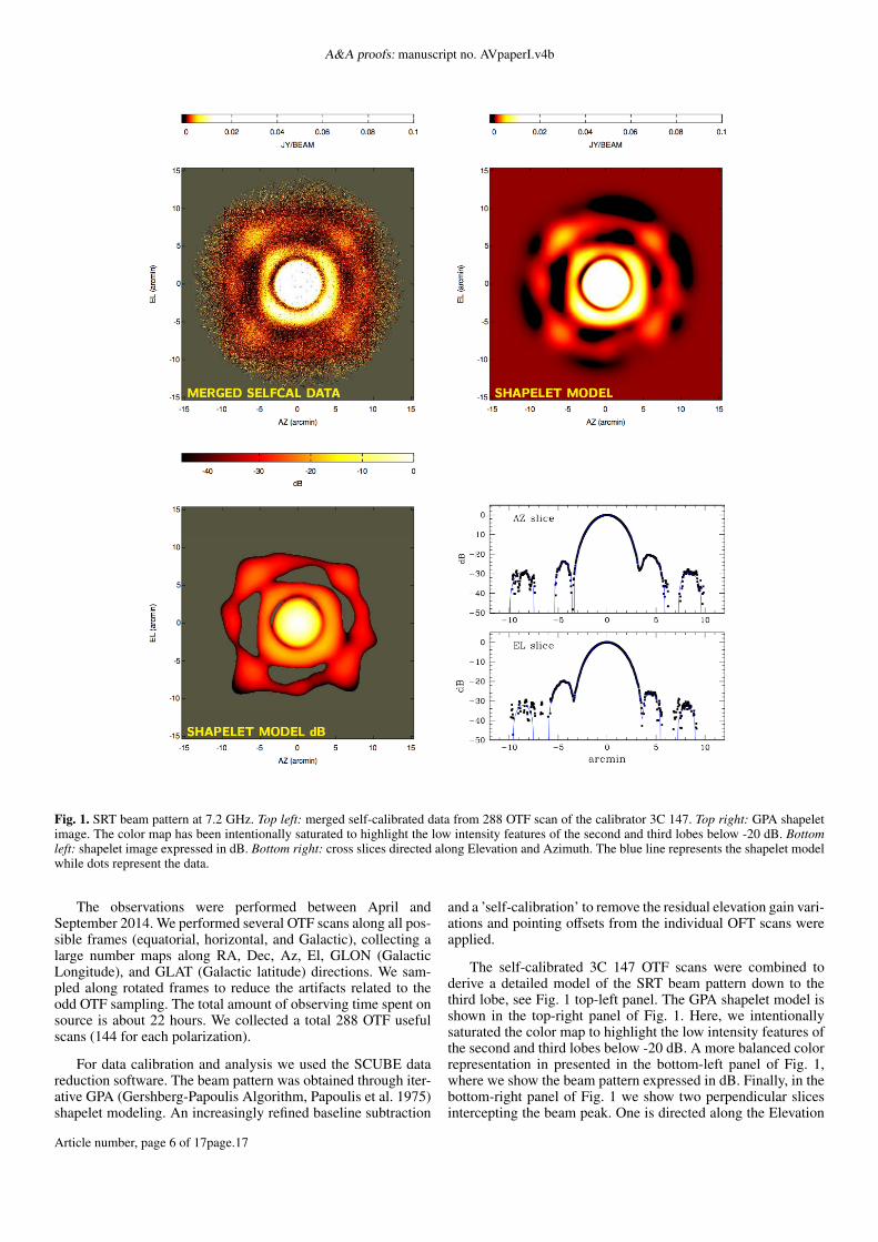
Fig. 1. SRT beam pattern at 7.2 GHz. Top left: merged self-calibrated data from 288 OTF scan of the calibrator 3C 147. Top right: GPA shapeletimage. The color map has been intentionally saturated to highlight the low intensity features of the second and third lobes below -20 dB. Bottomleft: shapelet image expressed in dB. Bottom right: cross slices directed along Elevation and Azimuth. The blue line represents the shapelet modelwhile dots represent the data.

The observations were performed between April andSeptember 2014. We performed several OTF scans along all pos-sible frames (equatorial, horizontal, and Galactic), collecting alarge number maps along RA, Dec, Az, El, GLON (GalacticLongitude), and GLAT (Galactic latitude) directions. We sam-pled along rotated frames to reduce the artifacts related to theodd OTF sampling. The total amount of observing time spent onsource is about 22 hours. We collected a total 288 OTF usefulscans (144 for each polarization).

For data calibration and analysis we used the SCUBE datareduction software. The beam pattern was obtained through iter-ative GPA (Gershberg-Papoulis Algorithm, Papoulis et al. 1975)shapelet modeling. An increasingly refined baseline subtraction

and a ’self-calibration’ to remove the residual elevation gain vari-ations and pointing offsets from the individual OFT scans wereapplied.

The self-calibrated 3C 147 OTF scans were combined toderive a detailed model of the SRT beam pattern down to thethird lobe, see Fig. 1 top-left panel. The GPA shapelet model isshown in the top-right panel of Fig. 1. Here, we intentionallysaturated the color map to highlight the low intensity features ofthe second and third lobes below -20 dB. A more balanced colorrepresentation in presented in the bottom-left panel of Fig. 1,where we show the beam pattern expressed in dB. Finally, in thebottom-right panel of Fig. 1 we show two perpendicular slicesintercepting the beam peak. One is directed along the Elevation



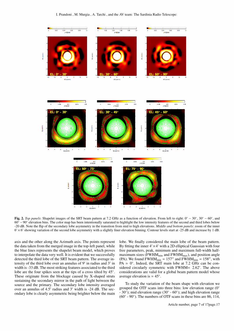
Fig. 2. Top panels: Shapelet images of the SRT beam pattern at 7.2 GHz as a function of elevation. From left to right: 0◦ − 30◦, 30◦ − 60◦, and60◦ − 90◦ elevation bins. The color map has been intentionally saturated to highlight the low intensity features of the second and third lobes below-20 dB. Note the flip of the secondary lobe asymmetry in the transition from mid to high elevations. Middle and bottom panels: zoom of the inner6′ × 6′ showing variation of the second lobe asymmetry with a slightly finer elevation binning. Contour levels start at -25 dB and increase by 1 dB.

axis and the other along the Azimuth axis. The points representthe data taken from the merged image in the top-left panel, whilethe blue lines represents the shapelet beam model, which provesto interpolate the data very well. It is evident that we successfullydetected the third lobe of the SRT beam pattern. The average in-tensity of the third lobe over an annulus of 9′ in radius and 3′ inwidth is -33 dB. The most striking features associated to the thirdlobe are the four spikes seen at the tips of a cross tilted by 45◦.These originate from the blockage caused by X-shaped strutssustaining the secondary mirror in the path of light between thesource and the primary. The secondary lobe intensity averagedover an annulus of 4.5′ radius and 3′ width is -24 dB. The sec-ondary lobe is clearly asymmetric being brighter below the main

lobe. We finally considered the main lobe of the beam pattern.By fitting the inner 4′×4′ with a 2D elliptical Gaussian with fourfree parameters, peak, minimum and maximum full-width half-maximum sizes (FWHMmin and FWHMmax), and position angle(PA). We found FWHMmin = 157′′ and FWHMmin = 158′′, withPA ' 0◦. Indeed, the SRT main lobe at 7.2 GHz can be con-sidered circularly symmetric with FWHM= 2.62′. The aboveconsiderations are valid for a global beam pattern model whoseaverage elevation is ' 45◦.

To study the variation of the beam shape with elevation wegrouped the OTF scans into three bins: low elevation range (0◦- 30◦); mid elevation range (30◦ - 60◦); and high elevation range(60◦ - 90◦). The numbers of OTF scans in these bins are 86, 114,



and 88, respectively, for a total of 288 images. All OTF scansin each of the three elevation bins were processed separately.The shapelet images for the three bins at low, mid, and high el-evations are shown in Fig. 2 (top-panels). These images have asomewhat lower sensitivity but it is clear that the beam patternvaries significantly with elevation. The most important effect isthe behavior of the secondary lobe structure at high elevations.In particular, we observe a flip of the asymmetry around an el-evation of 60◦. At elevation higher than 60◦ the brightest partof the secondary lobe is observed above the main lobe, while itis observed below it at mid and low elevations. A zoom of theinner 6′ × 6′ showing variations of the second lobe asymmetrywith a slightly finer elevation binning is presented in the middleand bottom panels of Fig. 2.

4.3. Fine Characterization of the Gain Curve

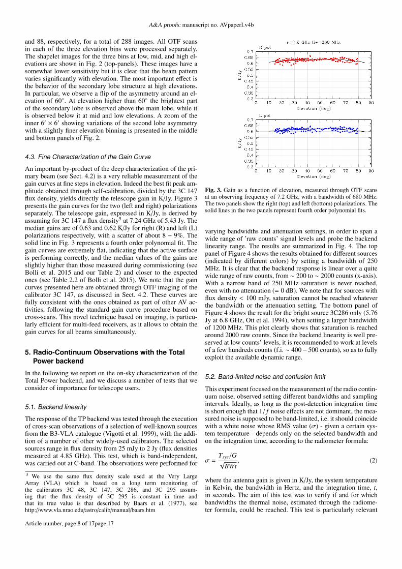
An important by-product of the deep characterization of the pri-mary beam (see Sect. 4.2) is a very reliable measurement of thegain curves at fine steps in elevation. Indeed the best fit peak am-plitude obtained through self-calibration, divided by the 3C 147flux density, yields directly the telescope gain in K/Jy. Figure 3presents the gain curves for the two (left and right) polarizationsseparately. The telescope gain, expressed in K/Jy, is derived byassuming for 3C 147 a flux density5 at 7.24 GHz of 5.43 Jy. Themedian gains are of 0.63 and 0.62 K/Jy for right (R) and left (L)polarizations respectively, with a scatter of about 8 − 9%. Thesolid line in Fig. 3 represents a fourth order polynomial fit. Thegain curves are extremely flat, indicating that the active surfaceis performing correctly, and the median values of the gains areslightly higher than those measured during commissioning (seeBolli et al. 2015 and our Table 2) and closer to the expectedones (see Table 2.2 of Bolli et al. 2015). We note that the gaincurves presented here are obtained through OTF imaging of thecalibrator 3C 147, as discussed in Sect. 4.2. These curves arefully consistent with the ones obtained as part of other AV ac-tivities, following the standard gain curve procedure based oncross-scans. This novel technique based on imaging, is particu-larly efficient for multi-feed receivers, as it allows to obtain thegain curves for all beams simultaneously.

5. Radio-Continuum Observations with the TotalPower backend

In the following we report on the on-sky characterization of theTotal Power backend, and we discuss a number of tests that weconsider of importance for telescope users.

5.1. Backend linearity

The response of the TP backend was tested through the executionof cross-scan observations of a selection of well-known sourcesfrom the B3-VLA catalogue (Vigotti et al. 1999), with the addi-tion of a number of other widely-used calibrators. The selectedsources range in flux density from 25 mJy to 2 Jy (flux densitiesmeasured at 4.85 GHz). This test, which is band-independent,was carried out at C-band. The observations were performed for

5 We use the same flux density scale used at the Very LargeArray (VLA) which is based on a long term monitoring ofthe calibrators 3C 48, 3C 147, 3C 286, and 3C 295 assum-ing that the flux density of 3C 295 is constant in time andthat its true value is that described by Baars et al. (1977), seehttp://www.vla.nrao.edu/astro/calib/manual/baars.htm

Fig. 3. Gain as a function of elevation, measured through OTF scansat an observing frequency of 7.2 GHz, with a bandwidth of 680 MHz.The two panels show the right (top) and left (bottom) polarizations. Thesolid lines in the two panels represent fourth order polynomial fits.

varying bandwidths and attenuation settings, in order to span awide range of ’raw counts’ signal levels and probe the backendlinearity range. The results are summarized in Fig. 4. The toppanel of Figure 4 shows the results obtained for different sources(indicated by different colors) by setting a bandwidth of 250MHz. It is clear that the backend response is linear over a quitewide range of raw counts, from ∼ 200 to ∼ 2000 counts (x-axis).With a narrow band of 250 MHz saturation is never reached,even with no attenuation (= 0 dB). We note that for sources withflux density < 100 mJy, saturation cannot be reached whateverthe bandwidth or the attenuation setting. The bottom panel ofFigure 4 shows the result for the bright source 3C286 only (5.76Jy at 6.8 GHz, Ott et al. 1994), when setting a larger bandwidthof 1200 MHz. This plot clearly shows that saturation is reachedaround 2000 raw counts. Since the backend linearity is well pre-served at low counts’ levels, it is recommended to work at levelsof a few hundreds counts (f.i. ∼ 400− 500 counts), so as to fullyexploit the available dynamic range.

5.2. Band-limited noise and confusion limit

This experiment focused on the measurement of the radio contin-uum noise, observed setting different bandwidths and samplingintervals. Ideally, as long as the post-detection integration timeis short enough that 1/ f noise effects are not dominant, the mea-sured noise is supposed to be band-limited, i.e. it should coincidewith a white noise whose RMS value (σ) - given a certain sys-tem temperature - depends only on the selected bandwidth andon the integration time, according to the radiometer formula:

σ =Tsys/G√

BWt, (2)

where the antenna gain is given in K/Jy, the system temperaturein Kelvin, the bandwidth in Hertz, and the integration time, t,in seconds. The aim of this test was to verify if and for whichbandwidths the thermal noise, estimated through the radiome-ter formula, could be reached. This test is particularly relevant



Fig. 4. Source (baseline-subtracted) amplitude vs peak (source + base-line) level, both expressed in raw counts. Increasing raw counts on bothaxes reflect decreasing attenuation setting down to 0 dB. Top panel: Testperformed with 250 MHz bandwidth at a central observing frequencyof 7.25 GHz. Different sources are indicated by different colors. Bottompanel: Test performed with 1500 MHz bandwidth at a central observ-ing frequency of 6.8 GHz. Here only the bright source 3C286 (5.76 Jy at6.8 GHz, Ott et al. 1994) is shown, to highlight the levels of raw countswhere saturation is reached.

for the Total Power, as analogical backends do not allow an ef-ficient removal of RFI-affected data, and this can easily resultin increased noise levels, especially when large bandwidths areused.

The experiment was performed at both C- and K-bands. Theobserving frequencies were set so as to minimize the presence ofRFI. At C-band we set the low end of the bandwidth at 7 GHz,because of the presence of several strong RFI in the 5.7-6.9 GHzrange (see Bolli et al. 2015). The K-band is less affected by RFI,and we set the low end of the bandwidth at 24 GHz. We ac-quired data employing different setups: we varied the bandwidthfrom 250 to 1200 MHz, while data sampling ranged from 10to 80 ms. The subsequent noise RMS measurements were per-formed over various time windows (respectively lasting 1 s, 2 s,4 s) in order to reveal possible effects and instabilities at differenttime scales. Figure 5 shows the results for C-band (left panels)and K-band (right panels), in terms of the measured observed-to-expected RMS ratio, for either 2 s (top) or 4 s (bottom) timewindows. The 1 s window leads to poor statistics, as only a fewsamples are available - especially for the longer integrations. Allplots clearly show a band-related increase of the noise ratio, with

Fig. 5. Ratio of measured over expected noise as a function of sam-pling interval for different bandwidths (blue circles=250 MHz, greensquares=680 MHz, red diamonds=1200 MHz). The noise RMS is mea-sured (and estimated) over different time windows. Here we show theresults for 2 s (top) and 4 s (bottom) time windows. The experiment wasperformed at both C- (left panels) and K-bands (right panels).

the measured noise very close to the expected one for the small-est bandwidth (250 MHz), and getting a factor of 1.5 − 2 largergoing to 1200 MHz bandwidths. This is probably due to low-level RFIs, whose impact on continuum observations gets largerfor wider bandwidths, as more polluting signals are likely tobe gathered in a larger frequency range. This increase is morepronounced at C-band, as indeed RFI pollution affects this bandmore severely. We also note a trend for an increasing noise ratiogoing from 2 to 4 s time windows. This is probably due to thefact that the 4 s window starts to be affected by instabilities andgain drifts, leading to a measured signal which is not anymorepure white noise. These measurements allowed us to confirmthat band-limited noise can be reached by the TP, at least forsmall bandwidths, and that the effect of RFIs can be kept undercontrol, for an appropriate setting of the observing frequency.

Another important parameter that needs to be taken into ap-propriate account when planning observations is the time neededto reach the desired sensitivity. With this test we intended to ver-ify if the noise decreases with integration time (t) following theexpected 1/

√t law of the radiometer formula (see Eq. 2). The

experiment was performed at C-band, where the system tem-perature is very stable over a wide range of elevations (20-80◦),and the active surface provides very stable gains at all elevations(see Bolli et al. 2015). This means that variations of the tele-scope performance parameters with elevation do not affect ourmeasurements. The observations were carried out at a centralobserving frequency of 7.5 GHz with a bandwidth of 250 MHz,and consisted in repeated back-forth OTF scans along RA, ac-quired over a selected "empty sky" strip. This was chosen withina deeply-mapped area of the 10C survey (Ami Consortium 2011;more specifically, the strip was centered in RA=00h27m00ss,Dec=+31◦35’00" and it developed for a total RA span of 0.5◦.No sources having flux density greater than 0.1 mJy at 10 GHzare known to exist in this strip. The scans were inspected, flagged



Confusion limit measurement

1 10 100 1000Integration (s/beam)

0.1

1.0

RM

S −

(mJy

/bea

m)

Fig. 6. RMS noise as a function of increasing integration time. Theoblique solid line shows the expected trend according to the radiome-ter formula. The parallel dot-dashed line corresponds to the theoreticalnoise increased by 25%. The horizontal dot-dashed line shows the mea-sured confusion limit.

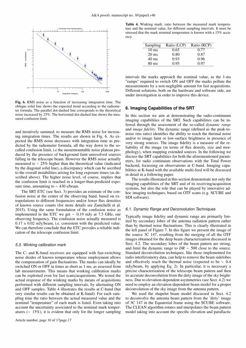
and iteratively summed, to measure the RMS noise for increas-ing integration times. The results are shown in Fig. 6. As ex-pected the RMS noise decreases with integration time as pre-dicted by the radiometer formula, all the way down to the so-called confusion limit, i.e the unsurmountable noise plateau pro-duced by the presence of background faint unresolved sourcesfalling in the telescope beam. However the RMS noise actuallymeasured is ∼ 25% higher than the theoretical value (indicatedby the diagonal solid line), a discrepancy which can be ascribedto the overall instabilities arising for long exposure times (as de-scribed above). The higher noise level, of course, implies thatthe confusion limit is reached in a longer-than-predicted expo-sure time, amounting to ∼ 430 s/beam.

The SRT ETC (see Sect. 3) provides an estimate of the con-fusion noise at the center of the observing band, based on ex-trapolations to different frequencies and/or lower flux densitiesof known source counts (for more details see Zanichelli et al.2015). Using the same formulation of the confusion noise asimplemented in the ETC we get ∼ 0.19 mJy at 7.5 GHz, ourobserving frequency. The confusion noise actually measured is0.17 ± 0.02 mJy/beam, i.e. consistent with the predicted value.We can therefore conclude that the ETC provides a reliable indi-cation of the telescope confusion limit.

5.3. Winking calibration mark

The C- and K-band receivers are equipped with fast-switchingnoise diodes of known temperature whose employment allowsthe compensation of gain fluctuations. The marks can ideally beswitched ON or OFF in times as short as 1 ms, as assessed fromlab measurements. This means that winking calibration markscan be exploited even for fast scans/acquisitions. We tested theactual response of the winking marks by means of acquisitionsperformed with different sampling intervals, by alternating ONand OFF samples. Table 4 illustrates the results at C-band (butvery similar results can be obtained at K-band). For each sam-pling time the ratio between the actual measured value and thenominal "temperature" of each mark is listed. Even taking intoaccount the uncertainty associated to the nominal mark temper-atures (∼ 15%), it is evident that only for the longer sampling

Table 4. Winking mark: ratio between the measured mark tempera-ture and the nominal value, for different sampling intervals. It must bestressed that the mark nominal temperature is known with a 15% accu-racy.

Sampling Ratio (LCP) Ratio (RCP)10 ms 0.65 0.7720 ms 0.80 0.8740 ms 0.93 0.9680 ms 0.95 0.97

intervals the marks approach the nominal value, as the 1-ms"ramps" required to switch ON and OFF the marks pollute themeasurements by a non-negligible amount for fast acquisitions.Different solutions, both on the hardware and software side, areunder investigation in order to improve this device.

6. Imaging Capabilities of the SRT

In this section we aim at demonstrating the radio-continuumimaging capabilities of the SRT. Such capabilities can be in-ferred through the assessment of the so-called dynamic rangeand image fidelity. The dynamic range (defined as the peak-to-noise rms ratio) identifies the ability to reach the thermal noiseand/or to image faint or low-surface brightness in presence ofvery strong sources. The image fidelity is a measure of the re-liability of the image (in terms of flux density, size and mor-phology), when mapping extended sources. In the following wediscuss the SRT capabilities for both the aforementioned param-eters, for radio continuum observations with the Total Powerbackend, focussing on observations at C-band. Imaging capa-bilities at K-band with the available multi-feed will be discussedin detail in a following paper.

The results illustrated in this section demonstrate not only theimaging capabilities of the SRT and of its receiving/acquisitionsystems, but also the role that can be played by innovative ad-hoc imaging techniques, based on OTF scans (e.g. SCUBE andSDI software).

6.1. Dynamic Range and Deconvolution Techniques

Typically image fidelity and dynamic range are primarily lim-ited by secondary lobes of the antenna radiation pattern ratherthan by thermal noise fluctuations. This is clearly illustrated inthe left panel of Figure 7. In this figure we present the image ofthe source 3C 147, resulting from the merging of all the OTFimages obtained for the deep beam characterization discussed inSect. 4.2. The secondary lobes of the beam pattern are strong,and limit the dynamic range to DR ∼ 500 close to the source.Standard deconvolution techniques, like those implemented forradio interferometry data, can help to remove the beam sidelobesand effectively reach the thermal noise (expected to be ∼ 0.4mJy/beam, by applying Eq. 2). In particular, it is necessary aprecise characterization of the telescope beam pattern and thenits accurate deconvolution from the dirty image of the sky bright-ness. Due to elevation-dependent asymmetries (see Sect. 4.2) weneed to employ an elevation-dependent beam model for a properdeconvolution of the sky image from the antenna pattern.

We used the shapelet beam model discussed in Sect. 4.2to deconvolve the antenna beam pattern from the ’dirty’ imageof 3C 147 in the Equatorial frame using the SCUBE software.The CLEAN algorithm rotates and interpolates the beam patternmodel taking into account the specific elevation and parallactic



Fig. 7. Left panel: ’Dirty’ image of 3C 147 resulting from the combi-nation of all OTF scans achieved for the characterization of the beam(see Sect. 4.2). Close to the source the dynamic range is limited toDR ∼ 500, due to the strong secondary lobes. Right panel: CLEANedimage restored with a circular Gaussian with FWHM beam of 2.6′. Themeasured noise r.m.s. is now 0.4 mJy/b and the dynamic range increasesto DR = 13350. The restoring beam is shown in the bottom-right cor-ner. In both panels contours starts from 3σ and increase by a factor of2. One negative contour level is traced at −3σ in red.

angle for each individual data point. For 3C 147 we measure apeak flux density of 5.34 Jy on the cleaned imaged, very closeto the expected flux density at 7.2 GHz of 5.43 Jy (on the scaleof Baars et al. 1977, see also Sect. 4.2). This corresponds to afractional difference < 1%. CLEAN components are convolvedwith a circular Gaussian with FWHM 2.6′ (shown in the bottom-right corner of the right panel) and restored to the residual image.Residuals have been tapered to 2.6′ to match the resolution ofthe restored clean component and to ensure an uniform resolu-tion across the field of view. The resulting image is shown in theright panel of Figure 7. The sidelobes are not an issue anymore,the noise is 0.4 mJy/beam and the dynamic range increases toDR = 13, 350. The improvement obtained with the deconvolu-tion is indeed very significant.

6.2. Dynamic Range: Extended Sources

In the previous section we dealt with the simplest case of a brightpoint source, here we want to determine the SRT capabilitiesto map large scale low-surface-brightness emission with brightpoint sources embedded in it. For this purpose, we observed twowell-known Galactic extended sources: the Omega Nebula andthe W3 molecular cloud complex.

The Omega Nebula and the W3 molecular cloud complex areconsidered among the brightest and most massive star-formingregions of our galaxy and are known to be very interesting exam-ples of maser and radio recombination line sources (se OH andMethanol maser measurements presented in Sect. 7). The con-tinuum radio emission from these objects is mostly due to free-free radiation emitted by Hydrogen ionized from the ultravioletphotons produced by young and massive stars. Both the OmegaNebula and W3 star-forming regions have been imaged as partof the commissioning of the Green Bank Telescope (GBT). Thismeans that we can directly compare the imaging capabilities oftwo state-of-the-art instruments at similar observing frequencyand resolution.

0 20 40 60 80 100JANSKY/BEAM

18 19 0018 20 0018 21 0018 22 00

-16 30 00

-16 15 00

-16 00 00

-15 45 00

RIGHT ASCENSION (J2000)

DECL

INAT

ION

(J20

00)

Fig. 8. Image of the Omega Nebula at 7.24 GHz. The field of view isabout 1o×1o. The noise is '7 mJy/beam and the SRT resolution is 2.6arcmin (SRT beam size at 7.24 GHz). The colour map has been biasedto highlight the low surface brightness emission. As a result, the centraland brightest part of the nebula, characterized by a surface brightness inthe range ' 3-100 Jy/beam, is saturated. Contour levels start from 100mJy/beam and increase by a factor

√2.

0 10 20 30JANSKY/BEAM

02 24 0002 28 0002 32 0002 36 00

60 30 00

61 00 00

61 30 00

62 00 00

RIGHT ASCENSION (J2000)

DECL

INAT

ION

(J20

00)

Fig. 9. Image of W3 at 7.24 GHz. The field of view is about 2o×2o.The noise is '4 mJy/beam and the resolution is 2.6 arcmin (SRT beamsize at 7.24 GHz). The colour map has been saturated to highlight thelow surface brightness emission. The brightest structure in the top-rightis the vast W3 molecular cloud complex which hosts the ultra-compactHII region W3.

We observed the two targets in the period October-November2014. We performed OTF maps along RA, DEC, GLON, GLAT,AZ, and EL directions. The data were acquired using the TotalPower backend at a central observing frequency of 7.24 GHzand with a bandwidth of 680 MHz. The main observational pa-rameters of both sources are listed in Table 5. The results arediscussed below.

The data of the Omega Nebula and the W3 molecular com-plex were reduced and analyzed using the SCUBE software. Wenote that to evaluate the robustness of our flux density mea-surements, we imaged also two well known calibrators, 3C 295and 3C 147, with an OTF mapping setup similar to the targets’one. These calibrators were analyzed through the same strategy



Table 5. Observational parameters for the 7.24 GHz observations of theGalactic extended sources discussed in Sects. 6.2 and 6.3.

Source Image Scan Sampling/ Totalsize speed Integration time Time

(deg2) (′/s) (ms) (h)Omega Nebula 1×1 3 10 6W3 2×2 6 10 83C 157 1.5×1.5 4 40 12.8W44 1.2×1 4 40 9.5

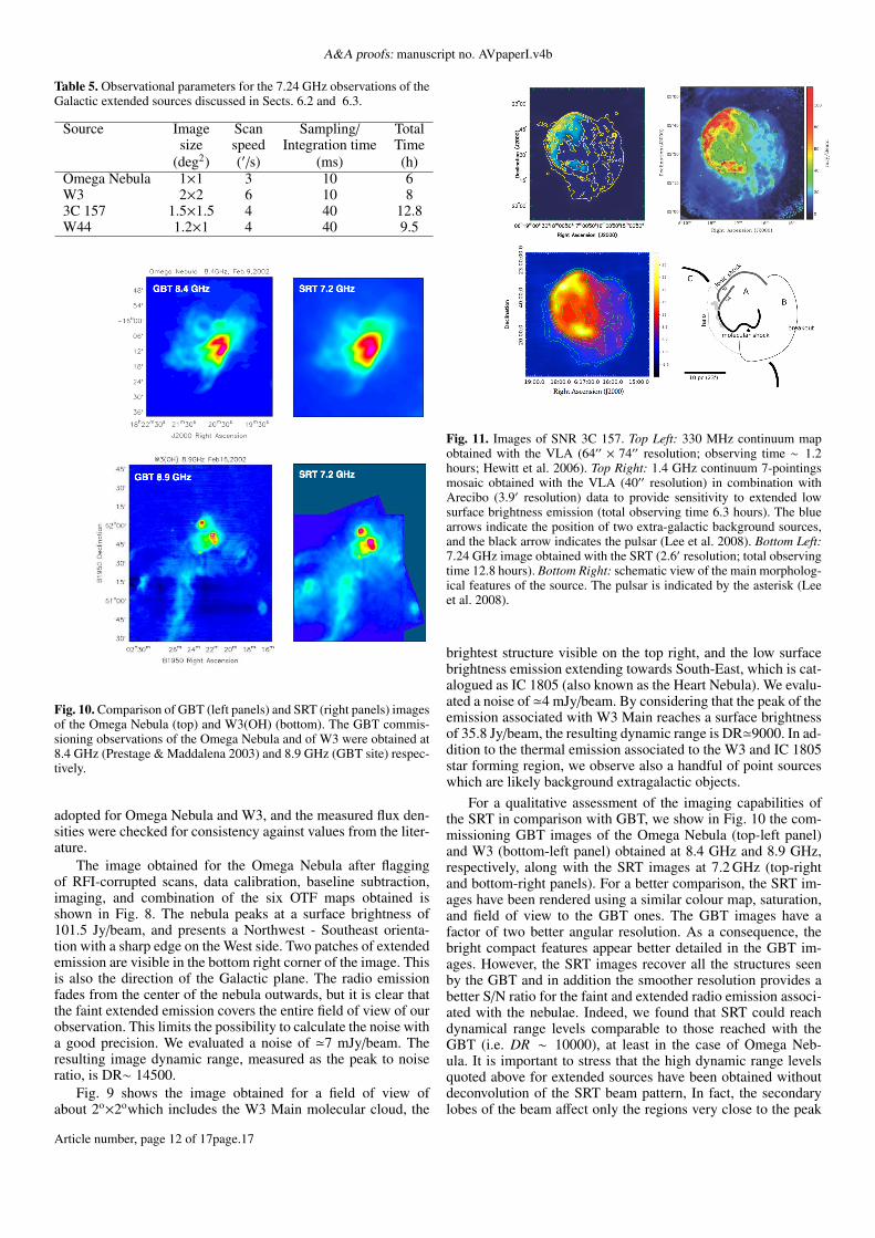
Fig. 10. Comparison of GBT (left panels) and SRT (right panels) imagesof the Omega Nebula (top) and W3(OH) (bottom). The GBT commis-sioning observations of the Omega Nebula and of W3 were obtained at8.4 GHz (Prestage & Maddalena 2003) and 8.9 GHz (GBT site) respec-tively.

adopted for Omega Nebula and W3, and the measured flux den-sities were checked for consistency against values from the liter-ature.

The image obtained for the Omega Nebula after flaggingof RFI-corrupted scans, data calibration, baseline subtraction,imaging, and combination of the six OTF maps obtained isshown in Fig. 8. The nebula peaks at a surface brightness of101.5 Jy/beam, and presents a Northwest - Southeast orienta-tion with a sharp edge on the West side. Two patches of extendedemission are visible in the bottom right corner of the image. Thisis also the direction of the Galactic plane. The radio emissionfades from the center of the nebula outwards, but it is clear thatthe faint extended emission covers the entire field of view of ourobservation. This limits the possibility to calculate the noise witha good precision. We evaluated a noise of '7 mJy/beam. Theresulting image dynamic range, measured as the peak to noiseratio, is DR∼ 14500.

Fig. 9 shows the image obtained for a field of view ofabout 2o×2owhich includes the W3 Main molecular cloud, the

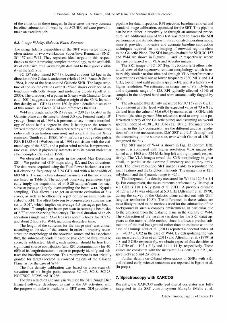
Fig. 11. Images of SNR 3C 157. Top Left: 330 MHz continuum mapobtained with the VLA (64′′ × 74′′ resolution; observing time ∼ 1.2hours; Hewitt et al. 2006). Top Right: 1.4 GHz continuum 7-pointingsmosaic obtained with the VLA (40′′ resolution) in combination withArecibo (3.9′ resolution) data to provide sensitivity to extended lowsurface brightness emission (total observing time 6.3 hours). The bluearrows indicate the position of two extra-galactic background sources,and the black arrow indicates the pulsar (Lee et al. 2008). Bottom Left:7.24 GHz image obtained with the SRT (2.6′ resolution; total observingtime 12.8 hours). Bottom Right: schematic view of the main morpholog-ical features of the source. The pulsar is indicated by the asterisk (Leeet al. 2008).

brightest structure visible on the top right, and the low surfacebrightness emission extending towards South-East, which is cat-alogued as IC 1805 (also known as the Heart Nebula). We evalu-ated a noise of '4 mJy/beam. By considering that the peak of theemission associated with W3 Main reaches a surface brightnessof 35.8 Jy/beam, the resulting dynamic range is DR'9000. In ad-dition to the thermal emission associated to the W3 and IC 1805star forming region, we observe also a handful of point sourceswhich are likely background extragalactic objects.

For a qualitative assessment of the imaging capabilities ofthe SRT in comparison with GBT, we show in Fig. 10 the com-missioning GBT images of the Omega Nebula (top-left panel)and W3 (bottom-left panel) obtained at 8.4 GHz and 8.9 GHz,respectively, along with the SRT images at 7.2 GHz (top-rightand bottom-right panels). For a better comparison, the SRT im-ages have been rendered using a similar colour map, saturation,and field of view to the GBT ones. The GBT images have afactor of two better angular resolution. As a consequence, thebright compact features appear better detailed in the GBT im-ages. However, the SRT images recover all the structures seenby the GBT and in addition the smoother resolution provides abetter S/N ratio for the faint and extended radio emission associ-ated with the nebulae. Indeed, we found that SRT could reachdynamical range levels comparable to those reached with theGBT (i.e. DR ∼ 10000), at least in the case of Omega Neb-ula. It is important to stress that the high dynamic range levelsquoted above for extended sources have been obtained withoutdeconvolution of the SRT beam pattern, In fact, the secondarylobes of the beam affect only the regions very close to the peak



of the emission in these images. In these cases the very accuratebaseline subtraction allowed by the SCUBE software proved tomake an excellent job.

6.3. Image Fidelity: Galactic Plane Sources

The image fidelity capabilities of the SRT were tested throughobservations of two well-known SuperNova Remnants (SNR):3C 157 and W44. They represent ideal targets in this respect,thanks to their interesting complex morphology, to the availabil-ity of extensive multi-wavelength data and to their good visibil-ity at the SRT site.

3C 157 (also named IC443), located at about 1.5 kpc in thedirection of the Galactic anticenter (Heiles 1984; Braun & Strom1986), is one of the best-studied Galactic SNR. The large struc-ture of the source extends over 0.75oand shows evidence of in-teractions with both atomic and molecular clouds (Snell et al.2005). The discovery of a pulsar in X-rays with Chandra (Olbertet al. 2001) suggests a core-collapse origin of the SNR. Its radioflux density at 1 GHz is about 160 Jy (for a detailed discussionof this source, see Green 2014 and references therein).

W44 is a bright radio SNR (S1 GHz ∼ 230 Jy) located in theGalactic plane at a distance of about 3.0 kpc. Formed nearly 104

yrs ago (Jones et al. 1993), it presents an asymmetric morphol-ogy of about half a degree in size. It belongs to the remnant’mixed morphology’ class, characterized by a highly filamentaryradio shell (synchrotron emission) and a central thermal X-rayemission (Smith et al. 1985). W44 harbors a young radio pulsarPSR B1853+01 (Wolszcan et al. 1991) consistent with the esti-mated age of the SNR, and a pulsar wind nebula. It represents arare case, since it physically interacts with its parent molecularcloud complex (Seta et al. 1998).

We observed the two targets in the period May-December2014. We performed OTF maps along RA and Dec directions.The data were acquired using the Total Power backend at a cen-tral observing frequency of 7.24 GHz and with a bandwidth of680 MHz. The main observational parameters of the two sourcesare listed in Table 5. The adopted observing parameters typi-cally imply the acquisition of >10-20 samples/beam for eachsubscan passage (largely oversampling the beam w.r.t. Nyquistsampling). This allows us to get an accurate evaluation of fluxerrors, as well as to efficiently reject outlier measurements as-cribed to RFI. The offset between two consecutive subscans wasset to 0.01o, which implies on average 4.5 passages per beam,and about 17 samples per beam per scan (assuming a beam sizeof 2.7′′ at our observing frequency). The total duration of an ob-servation (single map RA+Dec) was about 3 hours for 3C157,and about 2 hours for W44, including dead/slew time.

The length of the subscans (or the image size) was chosenaccording to the size of the source. In order to properly recon-struct the morphology of the observed source and its associatedflux, the subscan-dependent baseline (background flux) must becorrectly subtracted. Ideally, each subscan should be free fromsignificant source contribution (and RFI contamination) for 40-60% of its length/duration, in order to properly identify and sub-tract the baseline component. This requirement is not triviallygranted for targets located in crowded regions of the GalacticPlane, as for the case of W44.

The flux density calibration was based on cross-scan ob-servations of six bright point sources: 3C147, 3C48, 3C123,NGC7027, 3C295 and 3C286.

For data reduction and analysis we used the SDI (Single DishImager) software, developed as part of the AV activities, withthe purpose to make it available to SRT users. SDI provides a

pipeline for data inspection, RFI rejection, baseline removal andstandard image calibration, optimized for the SRT. This pipelinecan be run either interactively or through an automated proce-dure. An additional aim of this test was then to assess the SDIperformance and its robustness in its automated operation mode,since it provides innovative and accurate baseline subtractiontechniques required for the imaging of crowded regions closeto the Galactic Plane. The SDI images obtained for SNR 3C 157and W44 are shown in Figures 11 and 12 respectively, wherethey are compared with VLA and Arecibo images.

The SRT image of 3C 157 (Fig. 11, bottom left) offers a de-tailed view of the supernova remnant morphology, which is re-markably similar to that obtained through VLA interferometricobservations carried out at lower frequency (330 MHz and 1.4GHz, top left and right panels respectively), and at a factor 2− 4higher resolution. We estimated an image rms of 9.9 mJy/beamand a dynamic range of ∼125. RFI typically affected <10% ofsamples in the adopted band and were automatically flagged bySDI.

The integrated flux density measured for 3C 157 is 89.0±1.1Jy, consistent at a 2σ level with the expected value of 73 ± 8 Jy,derived from the value of 84.6±9.4 Jy measured at 4.8 GHz withUrumqi (the sino-german 25m telescope, used to carry out a po-larization survey of the Galactic plane) and assuming an overallspectral index of −0.38 ± 0.1 (Gao et al. 2011). The main uncer-tainties in this flux comparison are the different angular resolu-tions of the two measurements (2.6′ SRT and 9.5′ Urumqi) andthe uncertainty on the source size, over which Gao et al. (2011)integrated the flux.

The SRT image of W44 is shown in Fig. 12 (bottom left),where it is compared with higher resolution VLA images ob-tained at at 1465 and 324 MHz (top left and right panels respec-tively). The VLA images reveal the SNR morphology in greatdetail, in particular the extreme filamentary and clumpy emis-sion. The lower resolution SRT image is able to reproduce themain features and the brightest filaments. The image rms is 12.1mJy/beam and the dynamic range is ∼250.

The integrated flux density measured for W44 is 129.5 ± 1.4Jy. For comparison, the measurements performed by Urumqi at4.8 GHz is 118 ± 6 Jy (Sun et al. 2011). A previous estimateof 127 ± 13 Jy was obtained at 5.0 GHz (Altenhoff et al. 1979),during the survey of the Galactic plane carried out with GBT(angular resolution 10.8′). The differences in these values aremost likely related to the methods used for the subtraction of thebackground in such a complex environment, in particular dueto the emission from the Galactic plane in the vicinity of W44.The subtraction of the baseline (as done for the SRT data) ap-pears as the most reliable method since it allows a precise sub-traction of the real background rather than an estimate as in thecase of Urumqi. Sun et al. (2011) reported a spectral index ofα = −0.37 ± 0.02 in the case of W44. By extrapolating the val-ues measured by Sun et al. (2011) and Altenhoff et al. (1979) at4.8 and 5 GHz respectively, we obtain expected flux densities at7.2 GHz of ∼ 102 ± 5 Jy and 111 ± 11 Jy, respectively. Thesevalues are consistent with the measured flux density at SRT, re-spectively at 5 and 2σ levels.

Further details on C-band observations of SNRs with SRTand related early science outcomes are reported in Egron et al.(in prep.).

7. Spectroscopy with XARCOS

Recently, the XARCOS multi-feed digital correlator was fullyintegrated in the SRT control system Nuraghe (Melis et al.



Fig. 12. Images of SNR W44. Comparison of the map obtained withSRT (bottom left, 2.6′ resolution) with high-resolution images of theradio continuum at 1465 MHz (top left) and 324 MHz (top right, 13′′resolution) obtained with the VLA. The yellow point in the top rightimage indicates the position of the pulsar PSR B1853+01. The bottomright panel shows the 324 MHz image of the remnant (in blue) over-lapped to Spitzer 8 and 24 µm datasets (in green and red respectively;Castelletti et al. 2007).

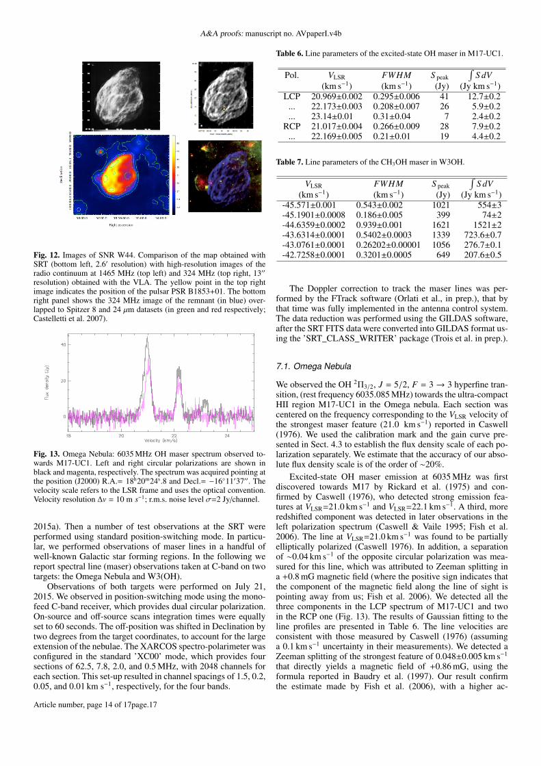
Fig. 13. Omega Nebula: 6035 MHz OH maser spectrum observed to-wards M17-UC1. Left and right circular polarizations are shown inblack and magenta, respectively. The spectrum was acquired pointing atthe position (J2000) R.A.= 18h20m24s.8 and Decl.= −16◦11′37′′. Thevelocity scale refers to the LSR frame and uses the optical convention.Velocity resolution ∆v = 10 m s−1; r.m.s. noise level σ=2 Jy/channel.

2015a). Then a number of test observations at the SRT wereperformed using standard position-switching mode. In particu-lar, we performed observations of maser lines in a handful ofwell-known Galactic star forming regions. In the following wereport spectral line (maser) observations taken at C-band on twotargets: the Omega Nebula and W3(OH).

Observations of both targets were performed on July 21,2015. We observed in position-switching mode using the mono-feed C-band receiver, which provides dual circular polarization.On-source and off-source scans integration times were equallyset to 60 seconds. The off-position was shifted in Declination bytwo degrees from the target coordinates, to account for the largeextension of the nebulae. The XARCOS spectro-polarimeter wasconfigured in the standard ’XC00’ mode, which provides foursections of 62.5, 7.8, 2.0, and 0.5 MHz, with 2048 channels foreach section. This set-up resulted in channel spacings of 1.5, 0.2,0.05, and 0.01 km s−1, respectively, for the four bands.

Table 6. Line parameters of the excited-state OH maser in M17-UC1.

Pol. VLSR FWHM S peak∫

S dV(km s−1) (km s−1) (Jy) (Jy km s−1)

LCP 20.969±0.002 0.295±0.006 41 12.7±0.2... 22.173±0.003 0.208±0.007 26 5.9±0.2... 23.14±0.01 0.31±0.04 7 2.4±0.2

RCP 21.017±0.004 0.266±0.009 28 7.9±0.2... 22.169±0.005 0.21±0.01 19 4.4±0.2

Table 7. Line parameters of the CH3OH maser in W3OH.

VLSR FWHM S peak∫

S dV(km s−1) (km s−1) (Jy) (Jy km s−1)

-45.571±0.001 0.543±0.002 1021 554±3-45.1901±0.0008 0.186±0.005 399 74±2-44.6359±0.0002 0.939±0.001 1621 1521±2-43.6314±0.0001 0.5402±0.0003 1339 723.6±0.7-43.0761±0.0001 0.26202±0.00001 1056 276.7±0.1-42.7258±0.0001 0.3201±0.0005 649 207.6±0.5

The Doppler correction to track the maser lines was per-formed by the FTrack software (Orlati et al., in prep.), that bythat time was fully implemented in the antenna control system.The data reduction was performed using the GILDAS software,after the SRT FITS data were converted into GILDAS format us-ing the ’SRT_CLASS_WRITER’ package (Trois et al. in prep.).

7.1. Omega Nebula

We observed the OH 2Π3/2, J = 5/2, F = 3→ 3 hyperfine tran-sition, (rest frequency 6035.085 MHz) towards the ultra-compactHII region M17-UC1 in the Omega nebula. Each section wascentered on the frequency corresponding to the VLSR velocity ofthe strongest maser feature (21.0 km s−1) reported in Caswell(1976). We used the calibration mark and the gain curve pre-sented in Sect. 4.3 to establish the flux density scale of each po-larization separately. We estimate that the accuracy of our abso-lute flux density scale is of the order of ∼20%.

Excited-state OH maser emission at 6035 MHz was firstdiscovered towards M17 by Rickard et al. (1975) and con-firmed by Caswell (1976), who detected strong emission fea-tures at VLSR=21.0 km s−1 and VLSR=22.1 km s−1. A third, moreredshifted component was detected in later observations in theleft polarization spectrum (Caswell & Vaile 1995; Fish et al.2006). The line at VLSR=21.0 km s−1 was found to be partiallyelliptically polarized (Caswell 1976). In addition, a separationof ∼0.04 km s−1 of the opposite circular polarization was mea-sured for this line, which was attributed to Zeeman splitting ina +0.8 mG magnetic field (where the positive sign indicates thatthe component of the magnetic field along the line of sight ispointing away from us; Fish et al. 2006). We detected all thethree components in the LCP spectrum of M17-UC1 and twoin the RCP one (Fig. 13). The results of Gaussian fitting to theline profiles are presented in Table 6. The line velocities areconsistent with those measured by Caswell (1976) (assuminga 0.1 km s−1 uncertainty in their measurements). We detected aZeeman splitting of the strongest feature of 0.048±0.005 km s−1

that directly yields a magnetic field of +0.86 mG, using theformula reported in Baudry et al. (1997). Our result confirmthe estimate made by Fish et al. (2006), with a higher ac-



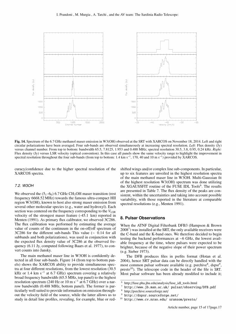
Fig. 14. Spectrum of the 6.7 GHz methanol maser emission in W3(OH) observed at the SRT with XARCOS on November 18, 2014. Left and rightcircular polarizations have been averaged. Four sub-bands are observed simultaneously at increasing spectral resolution. Left: Flux density (Jy)versus channel number. From top to bottom: bandwidth 65.5, 7.8125, 1.953 and 0.488 MHz; spectral resolution 30.5, 3.8, 0.95, 0.24 kHz. Right:Flux density (Jy) versus LSR velocity (optical convention). In this case all panels show the same velocity range to highlight the improvement inspectral resolution throughout the four sub-bands (from top to bottom: 1.4 km s−1, 170, 40 and 10 m s−1) provided by XARCOS.

curacy/confidence due to the higher spectral resolution of theXARCOS spectra.

7.2. W3OH

We observed the (51–60) 6.7 GHz CH3OH maser transition (restfrequency 6668.52 MHz) towards the famous ultra-compact HIIregion W3(OH), known to host also strong maser emission fromseveral other molecular species (e.g., water and hydroxyl). Eachsection was centered on the frequency corresponding to the VLSRvelocity of the strongest maser feature (-45.1 km) reported inMenten (1991). As primary flux calibrator, we observed 3C286.The flux calibration was performed by estimating the averagevalue of counts of the continuum in the on-off/off spectrum of3C286 for the different sub-bands This value (∼ 0.14 for allsubbands and both polarizations), was used in conjunction withthe expected flux density value of 3C286 at the observed fre-quency (6.11 Jy, computed following Baars et al. 1977), to con-vert counts into Jansky.

The main methanol maser line in W3OH is confidently de-tected in all four sub-bands. Figure 14 (from top to bottom pan-els) shows the XARCOS ability to provide simultaneous spec-tra at four different resolutions, from the lowest resolution (30.5kHz or 1.4 km s−1 at 6.7 GHz) spectrum covering a relativelybroad frequency bandwidth (65.5 MHz, top panel) to the highestresolution spectrum (240 Hz or 10 m s−1 at 6.7 GHz) over a nar-row bandwidth (0.488 MHz, bottom panel). The former is par-ticularly well suited to provide information on emission through-out the velocity field of the source, while the latter allows us tostudy in detail line profiles, revealing, for example, blue or red-

shifted wings and/or complex line sub-components. In particular,up to six features are unveiled in the highest resolution spectraof the main methanol maser line in W3OH. Multi-Gaussian fitof the highest resolution W3(OH) spectrum was done utilizingthe XGAUSSFIT routine of the FUSE IDL Tools6. The resultsare presented in Table 7. The flux density of the peaks are con-sistent, within the uncertainties and taking into account possiblevariability, with those reported in the literature at comparablespectral resolutions (e.g., Menten 1991).

8. Pulsar Observations

When the ATNF Digital Filterbank DFB3 (Hampson & Brown20087) was installed at the SRT, the only available receivers werethe C-band and the K-band ones. We therefore decided to begintesting the backend performances at ∼6 GHz, the lowest avail-able frequency at the time, where pulsars were expected to bebrighter, because of the negative slope of their power spectrum(e.g. Sieber 1973).

The DFB produces files in psrfits format (Hotan et al.2004), hence SRT pulsar data can be directly handled with themost common pulsar software available (e.g. psrchive8, dspsr9,presto10). The telescope code in the header of the file is SRT.Most pulsar software has been already modified to include it;

6 http://fuse.pha.jhu.edu/analysis/fuse_idl_tools.html7 http://www.jb.man.ac.uk/ pulsar/observing/DFB.pdf8 http://psrchive.sourceforge.net/9 http://dspsr.sourceforge.net/

10 http://www.cv.nrao.edu/ sransom/presto/



tempo11/tempo2 (Hobbs et al. 2006) one letter code for our tele-scope is z and the alias is srt.

C-band observation tests started in June 2013 on a smallnumber of pulsars and continued until the installation of the L-Pband coaxial receiver. Results on the more extensive observa-tions performed at these lower frequencies will be reported else-where.

Backend configurations tested with these first C-band obser-vations are listed in table 8: both folding mode and search modeobservations, with sampling times down to xx µs, were success-fully performed. Data acquisition was carried out initially usingthe built-in TKDS graphical interface, now fully superseded bythe new data acquisition system SEADAS (see Sect. 3).

Table 8. DFB configurations tested for C-band observations. The threenumbers of the folding mode configurations refer to, in the order, timebins in the pulse profile, bandwidth in MHz and number of frequencychannels, while for the search mode configurations they represent band-width and channels.

Folding mode Search modepdfb4_1024_1024_1024 srch_1024_512pdfb4_1024_1024_256 srch_512_128pdfb4_1024_512_512pdfb4_256_1024_512pdfb4_512_1024_1024pdfb4_512_1024_512pdfb4_512_512_512

Table 9 lists the pulsars observed, the number of observationsperformed, the average length of the pointings and the averagesignal-to-noise ratio of the integrated pulse profile. In the lastcolumn, an estimate of the flux density calculated on the basisof a modification of the radiometer equation for pulsars (see e.g.Manchester et al. 2001) is reported. In the first part of the ta-ble we lists bright long period pulsars while in the second partwe summarize the observations performed on four millisecondpulsars (MSPs) for which a flux density measurement at similarfrequency was reported in the literature (Kramer et al. 1999).

Table 9. Pulsar observed at C-band. In the columns we report pulsarnames, number of observations, average length of the observations, av-erage signal-to-noise ratio achieved and flux density estimate at 6 GHz.In the top part of the table we list long period, bright pulsars while inthe bottom part we list the observed millisecond pulsars.

PSR name Nobs Tobs (s) S/N S6000 (mJy)B0329+54 21 304 124 2.5B0355+54 6 666 281 5.2J1852-0635 2 115 65 6.7B1929+10 3 164 122 4.6B2020+28 1 510 30 0.7B2021+51 6 303 244 4.2

J1713+0747 1 1830 22 0.2B1855+09 1 930 13 0.4B1937+21 1 630 12 0.2J2145-0750 2 1365 10 0.1

Figure 15 shows the integrated pulse profiles of the smallsample of observed pulsars. In the top part of the plot we showthe profiles for the long period bright pulsars, while in the bottompart those for four MSPs, together with the pulse profile obtained

11 http://tempo.sourceforge.net/

with the Effelsberg radio telescope, for comparison (Kramer etal. 1999).

Flux densities and pulse profiles are, within the uncertain-ties (& 30% for the flux densities estimated with the radiometerequation and using the tabulated value of the system tempera-ture), consistent with what is found in the literature.

We are now finalizing tests observations of the noise diodefor which only recently an optical link was added that allows theDFB to directly switch its signal on and off. This will allow toobtain calibrated polarization and flux measurements in the verynear future.

9. Conclusions and Future PerspectivesAcknowledgements. F. Loi gratefully acknowledges the Sardinia Regional Gov-ernment for financial support of her PhD scholarship (P.O.R. Sardegna F.S.E.Operational Programme of the Autonomous Region of Sardinia, European SocialFund 2007 − 2013 - Axis IV Human Resources, Objective l.3, Line of Activityl.3.1.). M. Pilia was supported by the Sardinia Regional Government through theproject "Development of a Software Tool for the Study of Pulsars from Radio toGamma-rays using Multi-mission Data" (CRP-25476). V. Vacca was supportedby the DFG Forschengruppe 1254 "Magnetisation of Interstellar and Intergalac-tic Media: The Prospects of Low-Frequency Radio Observations". The develop-ment of the SARDARA backend has been funded by the Autonomous Regionof Sardinia (RAS) using resources from the Regional Law 7/2007 "Promotion ofthe scientific research and technological innovation in Sardinia" in the contextof the research project CRP-49231 (year 2011): "High resolution sampling ofthe Universe in the radio band: an unprecedented instrument to understand thefundamental laws of the nature".

ReferencesAltenhoff W.J., Downes D., Pauls T. and Schraml J. 1979, A&AS, 35, 23AMI consortium: Davies et al., 2011, MNRAS, 415, 2708ABaars, Genzel, Pauliny-Toth, Witzel 1977, A&A, 61, 99Bartolini M., Libardi P., Righini S. 2013, IRA Technical Report, IRA 466-13,

also available at http://www.srt.inaf.itBassa C. G., Janssen G. H., Karuppusamy R., et al. 2016, MNRAS, in press,

arXiv:1511.06597Baudry, A., Desmurs, J. F., Wilson, T. L., & Cohen, R. J. 1997, A&A, 325, 255BBolli P., Orlati A., Stringhetti L., et al. 2015, Journal of Astronomical Instrumen-

tation, in pressBraun R. & Strom R.G. 1986, A&A, 164, 193Burton M.G., Geballe T.R., Brand P.W.J.L. and Webster A.S. 1988, MNRAS,

231, 617Buttu M., Orlati A., Zacchiroli G., et al. 2012, Proceedings SPIE, Vol. 8451, doi

10.1117/12.925387Castelletti G., Dubner G., Brogan C. and Kassim N.E. 2007, A&A, 471, 537Caswell, J. L., 1976, MNRAS, 177, 601CCaswell, J. L., & Vaile, R. A. 1995 MNRAS, 273, 328CCondon, J.J. (2009), NRAO PTCS Project Note 66.0Duin R.M. & van der Laan H. 1975, A&A, 40, 111Fish, V. L., Reid, M. J., Menten, K. M. & Pillai, T. 2006, A&A, 458, 485FFrail D.A., Giacani E.B., Goss W.M. & Dubner G. 1996, ApJ, 464, 165Gao X.Y., Han J.L., Reich W. et al. 2011, A&A, 5291, A159Green D.A. 2014, A Catalogue of Galactic Supernova Remnants (2014 May Re-

lease), www.mrao.cam.ac.uk/survey/snrsHeiles C. 1984, ApJS, 55, 585Hewitt J.W., Yusef-Zadeh F., Wardle M. et al. 2006, ApJ, 652, 1288Hobbs G. B., Edwards R. T., Manchester R. N., 2006, MNRAS, 369, 655Hotan A. W. , van Straten W., Manchester R.N, 2004, PASA, 21, 302Jones L. R., Smith A. & Angellini L. 1993, MNRAS, 265, 631Kramer M., Lange C., Lorimer D.R., Backer D. C., Xilouris K. M., Jessner A.,

Wielebinski R., 1999, ApJ, 526, 957Lee J.J., Koo B.C., Yun M.S., et al. 2008, AJ, 135, 796Melis A., Concu R., Trois A., et al. 2014, Internal Report N.36, Oss. Astr.

Cagliari (INAF)Melis A., et al. 2015, Internal Report N.52, Oss. Astr. Cagliari (INAF)Melis, A., Valente, G., Tarchi, A. et al., ?An infrastructure for multi-backend ob-

servations with the Sardinia Radio Telescope ?, Proc.SPIE Millimeter, Sub-millimeter, and Far-Infrared Detectors and Instrumentation for Astronomy,9153M, 2014

Menten, 1991, ApJ, 380, L75



Fig. 15. Pulse profiles for the pulsars observed at C-band with the DFB. The top two rows are long period, relatively bright pulsars. In the third rowwe show the four MSPs observed at the SRT and, for comparison, in the last row the same four MSPs as observed at 4.8 GHz with the Effelsbergradio telescope (plots adapted from Kramer et al. 1999).

Migoni C., Melis A., Fara A., et al., 2014, Internal Report N.42, Oss. Astr.Cagliari (INAF)

Nasyr F.T., Castiglia C., Buffa F., et al., 2013, Experimental Astronomy, DOI10.1007/s10686-013-9339-0

Olbert C.M., Clearfield C.R., Williams N.E. et al. 2001, ApJ, 554, 205Orlati A., Buttu M., Melis A., et al., 2012, Proceedings SPIE, Vol. 8451, id.

84512M-84512M-12Orlati A., et al., 2015, Proceedings of the 15th International Conference on Ac-

celerator and Large Experimental Control Systems (ICALEPCS 2015), inpress

Ott M., et al., 1994, A&A, 284, 331Paladini R., Burigana C., Davies R.D. et al. 2003, A&A, 397, 213Papoulis et al., 1975, ...Perrodin D., Concu R., Melis A., et al., 2014, Internal Report N.39, Oss. Astr.

Cagliari (INAF)Perrodin D., et al., 2016, Proceedings of 14th Marcel Grossmann Meeting, in

press

Petre R., Kuntz, K.D., Shelton R.L. 2002, ApJ, 579, 404Prandoni I., Melis A., Migoni C., et al. 2014, Procs. of 12th European VLBI

Network Symposium and Users Meeting, PoS(EVN 2014)046Prestage, R.M., & Maddalena, R.J., 2003, Proceedings SPIE, 4837, 944Reach W.T., Rho J. and Jarrett T.H. 2005, ApJ, 618, 297Rickard, L. J., Palmer, P., & Zuckerman, B. 1975 ApJ, 200, 6RRighini S., Orlati A., Poppi S., Buttu M., Migoni C., 2015, Nuraghe User Man-

ual, available at http://www.srt.inaf.itSeta M., Hasegawa T., Dame T.M. et al. 1998, ApJ, 505, 286Seta M., Hasegawa T., Sakamoto S. et al. 2004, AJ, 127, 1098Sieber W., 1973, A&A, 28, 237Smith A., Jones L.R., Watson M.G. et al. 1985, MNRAS, 217, 99Sun X. H., Reich P., Reich W. et al. 2011, A&A, 536, A83Tarchi A., Castangia P., Govoni F., et al. 2011, Internal Report N.27, Oss. Astr.

Cagliari (INAF)Vacca V., Iacolina M.N., Pellizzoni A., et al., 2013, Internal Report INAF-IRA

468/13



Vigotti M., et al., 1999, A&A Suppl. Ser., 139, 359Wolszcan A., Cordes J.M. & Dewey R.J. 1991, ApJ, 372, 99Zanichelli A. Righini S., Mack K.-H., et al., 2015, Internal Report INAF-IRA

487/15


The Sardinia Radio Telescope · The Sardinia Radio Telescope (SRT) is the new 64-m dish operated by...

Documents

Transcript of The Sardinia Radio Telescope · The Sardinia Radio Telescope (SRT) is the new 64-m dish operated by...