The SAMI Galaxy Survey: The cluster redshift survey, target selection … · · 2018-04-08target...

MNRAS 000, 1–28 (2016) Preprint 1 March 2017 Compiled using MNRAS LATEX style file v3.0

The SAMI Galaxy Survey: The cluster redshift survey,target selection and cluster properties.

M. S. Owers1,2⋆, J. T. Allen3,4, I. Baldry5, J. J. Bryant2,3,4, G. N. Cecil6, L. Cortese7,S. M. Croom3,4, S. P. Driver7, L. M. R. Fogarty3,4, A. W. Green2, E. Helmich8,J. T. A. de Jong8, K. Kuijken8, S. Mahajan9, J. McFarland10, M. B. Pracy3,A. G. S. Robotham7, G. Sikkema10, S. Sweet11, E. N. Taylor12, G. Verdoes Kleijn8,A. E. Bauer2, J. Bland-Hawthorn3, S. Brough2, M. Colless11, W. J. Couch2,R. L Davies13, M. J. Drinkwater4,14, M. Goodwin2, A. M. Hopkins2,I. S. Konstantopoulos2,15, C. Foster2, J. S. Lawrence2, N. P. F Lorente2,A. M. Medling11,16,17, N. Metcalfe18, S. N. Richards2,3,4, J. van de Sande4, N. Scott4,T. Shanks18, R. Sharp11, A. D. Thomas11 and C. Tonini19

Author affiliations are listed at the end of the paper

Accepted XXX. Received YYY; in original form ZZZ

ABSTRACTWe describe the selection of galaxies targeted in eight low redshift clusters(APMCC0917, A168, A4038, EDCC442, A3880, A2399, A119 and A85; 0.029 < z <0.058) as part of the Sydney-AAO Multi-Object integral field Spectrograph GalaxySurvey (SAMI-GS). We have conducted a redshift survey of these clusters using theAAOmega multi-object spectrograph on the 3.9m Anglo-Australian Telescope. Theredshift survey is used to determine cluster membership and to characterise the dy-namical properties of the clusters. In combination with existing data, the survey re-sulted in 21,257 reliable redshift measurements and 2899 confirmed cluster membergalaxies. Our redshift catalogue has a high spectroscopic completeness (∼ 94%) forrpetro ≤ 19.4 and clustercentric distances R < 2R200. We use the confirmed clus-ter member positions and redshifts to determine cluster velocity dispersion, R200,virial and caustic masses, as well as cluster structure. The clusters have virial masses14.25 ≤ log(M200/M⊙) ≤ 15.19. The cluster sample exhibits a range of dynamicalstates, from relatively relaxed-appearing systems, to clusters with strong indicationsof merger-related substructure. Aperture- and PSF-matched photometry are derivedfrom SDSS and VST/ATLAS imaging and used to estimate stellar masses. These esti-mates, in combination with the redshifts, are used to define the input target cataloguefor the cluster portion of the SAMI-GS. The primary SAMI-GS cluster targets haveR <R200, velocities |vpec| < 3.5σ200 and stellar masses 9.5 ≤ log(M

∗approx/M⊙)≤ 12.

Finally, we give an update on the SAMI-GS progress for the cluster regions.

Key words: galaxies: clusters: individual (APMCC0917, A168, A4038, EDCC442,A3880, A2399, A119, A85) – surveys – galaxies

1 INTRODUCTION

Toward the end of the last century, large-area red-shift surveys of statistically representative volumes of

⋆ E-mail: [email protected]

the nearby Universe were enabled by the advent ofwide-field, highly multiplexed fibre-fed spectrographs ca-pable of simultaneously collecting several hundred spec-tra. Surveys such as the 2-degree Field Galaxy Red-shift Survey (2dFGRS; Colless et al. 2001) and the SloanDigital Sky Survey (SDSS; York et al. 2000) have been

c⃝ 2016 The Authors

2 M. S. Owers et al.

pivotal both in characterising galaxy environment andin precisely defining how fundamental galaxy propertiessuch as luminosity, morphology, level of star formation,colour, gas-phase metallicity, stellar mass and nuclear ac-tivity correlate with the external environment on bothlarge (∼Mpc) and small (∼kpc) scales (Lewis et al. 2002;Norberg et al. 2002; Bell et al. 2003; Brinchmann et al.2004; Tremonti et al. 2004; Kauffmann et al. 2003b,a;Croton et al. 2005; Baldry et al. 2006; Peng et al. 2010).The dominant physical mechanisms governing these correla-tions have to date remained elusive.

Massive galaxy clusters are critical to understandingcorrelations between galaxy properties and environment;they host the densest environments where the effects ofmany of the physical mechanisms capable of galaxy trans-formation are strongest and, therefore, are expected to bemore readily observed. The potential mechanisms that canact to transform a cluster galaxy are well known (for anoverview, see Boselli & Gavazzi 2006). Interactions with thehot intracluster medium (ICM), such as ram-pressure andviscous stripping (Gunn & Gott 1972; Nulsen 1982) canremove the cold HI gas that fuels star formation or thehot gas halo reservoir (strangulation; Larson et al. 1980;Bekki et al. 2002), thereby leading to quenching of star for-mation with little impact on stellar structure. The effectof gravitational interactions, through either tides due tothe cluster potential (Byrd & Valtonen 1990; Bekki 1999),high-speed interactions between other cluster galaxies, orthe combination of both (harrassment; Moore et al. 1996),can impact both the distribution of old stars and the gas ina cluster galaxy, leading to transformations in morphologi-cal, kinematical, star-forming, and AGN properties of clustergalaxies (Byrd & Valtonen 1990; Bekki 1999). A large frac-tion of galaxies accreted onto clusters arrive in group-scalehalos (M200 < 1014M⊙) (McGee et al. 2009), where galaxymergers and interactions can pre-process a galaxy beforeit falls into a cluster. The amplitude of the effect of thesemechanisms is likely a function of parameters related to en-vironment including cluster halo mass, ICM properties, andcluster merger activity, as well as intrinsic galaxy propertiessuch as mass, morphology and gas content.

Deep, complete multi-object spectroscopic observationsof galaxy clusters allow the efficient collection of a large num-ber of spectroscopically confirmed cluster members. Thesemember galaxies are important kinematical probes of thecluster potential, allowing for relatively reliable dynamicalmass determinations based on common estimators such asthe velocity dispersion-based virial estimator (Girardi et al.1998), the escape velocity profile-based caustic technique(Diaferio 1999) and by fitting the 2D projected-phase-spacedistribution (Mamon et al. 2013) to name a few (for a com-prehensive analysis of different estimators, see; Old et al.2014, 2015). Many dynamical mass estimators assume spher-ical symmetry and dynamical equilibrium; these assump-tions are violated during major cluster mergers, thereby af-fecting the accuracy of mass measurements. Substructurerelated to cluster merger activity is routinely detected andcharacterised using the combined redshift and position in-formation for cluster members (Dressler & Shectman 1988;Colless & Dunn 1996; Pinkney et al. 1996; Pisani 1996;Ramella et al. 2007; Owers et al. 2009a,b, 2011a,b, 2013).Multi-object spectroscopic observations of clusters are there-

fore an important part of the tool-kit for characterising theglobal cluster environment, as well as the local environmen-tal properties surrounding a galaxy.

The observable imprint of the processes responsi-ble for environment-driven galaxy transformation can re-veal itself through spatially resolved spectroscopic ob-servations (e.g., Pracy et al. 2012; Merluzzi et al. 2013;Brough et al. 2013; Bekki 2014; Schaefer et al. 2017). There-fore, crucial to understanding which of the environment-related physical mechanisms are at play is knowledge ofthe resolved properties of galaxies spanning a range inmass, in combination with a detailed description of thegalaxy environment. The ongoing SAMI Galaxy Survey(SAMI-GS; Bland-Hawthorn et al. 2011; Croom et al. 2012;Bryant et al. 2014) is, for the first time, addressing thisissue by obtaining resolved spectroscopy for a large sam-ple of galaxies (Bryant et al. 2015; Allen et al. 2015). TheSAMI-GS is primarily targeting galaxies selected from theGalaxy And Mass Assembly survey (GAMA; Driver et al.2009, 2011; Liske et al. 2015), where deep, highly completespectroscopy allows high fidelity environment metrics tobe formulated (e.g., local density and group membershipRobotham et al. 2011; Brough et al. 2013). The SAMI-GSwill collect resolved spectroscopy for ∼ 2700 galaxies resid-ing in the GAMA regions. However, at the low redshifts tar-geted for the SAMI-GS, the volume probed by the GAMAregions contain few rare, rich cluster-scale halos found in thehigh mass portion of the mass function. To probe the fullrange of galaxy environments, the SAMI-GS is also target-ing ∼ 900 galaxies in the eight massive (M > 1014M⊙) clus-ters APMCC0917, A168, A4038, EDCC442, A3880, A2399,A119 and A85. For the majority of these clusters, only rel-atively shallow (r < 17.77, bJ < 19.45 for the SDSS and2dFGRS, respectively), intermediate completeness (∼ 80 −90%) spectroscopy was available (De Propris et al. 2002;Rines & Diaferio 2006). To address the disparity in redshiftdepth and completeness between the GAMA regions and thedense cluster regions, we have conducted a redshift survey ofthe cluster regions using the AAOmega multi-object spectro-graph on the 3.9m Anglo-Australian Telescope. The resultsand analysis of this survey are presented in this paper.

This paper provides details on the densest regionsprobed in the SAMI-GS: the cluster regions. In Section 2we outline the selection of the 8 cluster regions. In Section 3we outline the SAMI Cluster Redshift Survey (SAMI-CRS)which we use to define cluster properties (Section 4). Wethen outline the updated photometry for cluster galaxies andthe selection process for SAMI targets in the cluster regions.Finally, in Section 6, we outline the SAMI-GS progress in thecluster regions. Throughout this paper, we assume a stan-dard ΛCDM cosmology with H0 = 70 km s−1 Mpc−1,Ωm =0.3,ΩΛ = 0.7.

2 SELECTION OF SAMI CLUSTERS

Because the space density of massive clusters is low (n(M >1 × 1014 M⊙)∼ 10−5 Mpc−3; Murray et al. 2013)1 and theequatorial GAMA regions targeted by the SAMI Galaxy

1 http://hmf.icrar.org

MNRAS 000, 1–28 (2016)

The SAMI Galaxy Survey: The cluster redshift survey and target selection 3

Survey (hereafter SAMI-GS) probes 3.6 × 105 Mpc3 forz < 0.12, there will be too few massive clusters in themain SAMI-GS volume to probe the densest galaxy envi-ronments. Therefore, we utilise the wide-area 2dFGRS andSDSS to select a number of cluster regions to include in themain survey. The clusters are drawn from clusters within the2dFGRS from the catalogue of De Propris et al. (2002), andalso from clusters used in the Cluster Infall Regions in theSDSS (CIRS) survey of Rines & Diaferio (2006). The initialselection of the clusters was based on the following criteria:

• z ≤ 0.06 so that a significant portion of the galaxy lu-minosity/mass function can be probed in the cluster regions.For the limiting magnitude of the SAMI-CRS (r=19.4; Sec-tion 3) we probe ∼ 3 mag fainter than the knee in the clus-ter luminosity function (M∗

r = −20.6; Popesso et al. 2005).At this redshift, the stellar mass limit for the SAMI-GS islog10(M∗/M⊙)> 10 (Section 5.3). We therefore probe atleast a factor of 50 in stellar mass when compared with themost massive cluster galaxies (log10(M∗/M⊙) ∼ 11.6);

• Sufficient spectroscopy to clearly define boundariesin the peculiar velocity-radius phase-space diagrams (Fig-ure 8). For the clusters selected from the De Propris et al.(2002) catalogue, this criterion was achieved by selectingonly clusters with more than 50 members and where thespectroscopic completeness of the tile was > 70%. For theclusters selected from CIRS, we require that the infall pat-tern in the cluster velocity-radius phase-space diagram beclassified as “clean” in the visual classification scheme pro-vided by Rines & Diaferio (2006).

• R.A. in the range 20 − 10hr and declination < 5 deg.This requirement meant that the clusters were observablefor a significant portion of the night from the AAT dur-ing Semester B, which runs August to January. This con-straint meant that the clusters did no overlap in R.A. withthe GAMA portion of the SAMI-GS that is observed duringSemester A.

The above selection criteria resulted in 18 clusters in the2dFGRS Southern Galactic Pole region and 7 clusters fromCIRS. We re-analyse the 2dFGRS clusters by selecting mem-bers using the caustic technique (see Section 4.1), defin-ing R200 and velocity dispersion of galaxies within R200,σ200, (as described in Section 4.1). We make a furthercut of clusters with σ200 < 450 km s−1, which accordingto the scaling relation of Evrard et al. (2008) are likelyto have log10(M200/M⊙) < 14. The SAMI-GS is alreadywell-populated in this mass range (see Figure 11 inBryant et al. 2015). This leaves six 2dFGRS clusters; twoof these appeared to have irregular and non-Gaussian ve-locity distributions within R200 that may affect their dis-persion measurements and so they were removed from thefinal sample. We also remove a further 3 CIRS clusters: twowith σ200 < 450 km s−1 (where the σ200 values are givenin Rines & Diaferio 2006), and one for which all of theRines & Diaferio (2006) mass measures are log10(M/M⊙)< 14. The remaining eight clusters make up the final clustersample for the SAMI-GS: four from the 2dFGRS region andfour from CIRS. The selected clusters are listed in Table 1.

2 http://cosmocalc.icrar.org

3 THE SAMI CLUSTER REDSHIFT SURVEY

The target selection for the GAMA portion of the SAMI-GS sample benefits greatly from the deep, highly com-plete spectroscopy provided by the GAMA survey whichwas conducted on the 3.9m Anglo-Australian Telescope(Driver et al. 2011; Liske et al. 2015). This spectroscopyprobes galaxies with much lower stellar mass when com-pared with the SAMI survey limits, allowing for a robustdefinition of the environment surrounding the SAMI sur-vey galaxies (e.g., the GAMA group catalogue provided byRobotham et al. 2011). While the selection of the clustersfor the SAMI survey required some level of spectroscopy tobe available from the SDSS and 2dFGRS, both of these sur-veys only probe down to galaxies ∼ 2 magnitude brighterthan the GAMA survey limits, and do not have the samelevel of spectroscopic completeness, particularly in the densecluster cores. In order to provide a similar level of high-fidelity spectroscopy for the dense cluster regions, we con-ducted a redshift survey of the eight regions: the SAMICluster Redshift Survey (SAMI-CRS). In this section, wedescribe the SAMI-CRS.

3.1 Input catalogue for spectroscopic follow-up

3.1.1 VST/ATLAS survey photometry (APMCC0917,EDCC0442, A3880 and A4038)

Targets for the four clusters selected from the 2dFGRScatalogue (De Propris et al. 2002) were selected from pho-tometry provided by the VLT Survey Telescope’s AT-LAS (VST/ATLAS) survey which is described in detail inShanks et al. (2013, 2015). Briefly, u, g, r, i and z-band pho-tometric catalogues for fields with centres within 4.5R200

of the cluster centres were retrieved from the VST archiveat the Cambridge Astronomy Survey Unit3 (CASU). Thesedata were obtained prior to the public data release of theVST/ATLAS survey and the second-order corrections to thenight-to-night photometric zeropoints of the different point-ings (described in Shanks et al. 2015) had not yet been ap-plied. To apply these corrections, we followed a method simi-lar to that described in Shanks et al. (2015); we cross-matchunsaturated stars detected in the VST/ATLAS data withstars in the APASS4 photometric survey of bright stars thathave 10 < V < 17 and compare their magnitudes in the g, rand i−bands. Each of the separate gri VST/ATLAS cata-logues is then corrected by the mean difference between theAPASS and VST/ATLAS star magnitudes. This accountsfor both the night-to-night variations in zeropoints, as wellas converting VST/ATLAS Vega magnitudes onto the ABmagnitude system used by APASS. Since there are no corre-sponding u and z−band measurements in APASS, we deter-mine the corrections in those bands by minimising the offsetbetween the stellar locus of the VST/ATLAS (u − g) vs(g−r) and (r− i) vs (i−z) colour-colour diagrams and thatof SDSS-selected stars. The u- and z-band photometry wereonly used in the selection of spectrophotometric standardsdescribed in Bryant et al. (2015). The final parent photo-metric catalogues selected are based on the r-band detec-

3 http://casu.ast.cam.ac.uk/vstsp/imgquery/search4 https://www.aavso.org/apass

MNRAS 000, 1–28 (2016)


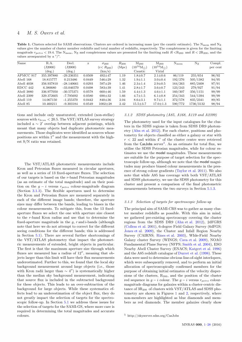
Table 1. Clusters selected for SAMI observations. Clusters are ordered in increasing mass (per the caustic estimate). The Nmem and NZ

values give the number of cluster member redshifts and total number of redshifts, respectively. The completeness is given for the limiting

magnitude rpetro < 19.4. The Nmem, NZ and completeness values are presented for the limiting radii R <R200 and R < 2R200, and thevalues areseparated by a ”/”.

Name R.A. Decl. z σ200 R200 M200 M200 Nmem NZ Compl.(J2000) (J2000) (r< R200) (Mpc) (1014M⊙) (1014M⊙) per cent(deg.) (deg.) (km/s) Caustic Virial

APMCC 917 355.397880 -29.236351 0.0509 492±47 1.19 1.8±0.7 2.1±0.6 86/119 255/654 96/92

Abell 168 18.815777 0.213486 0.0449 546±29 1.32 1.9±1.1 3.0±0.4 192/276 505/1382 94/95Abell 4038 356.937810 -28.140661 0.0293 597±29 1.46 2.3±1.4 2.9±0.5 164/263 885/2408 97/91EDCC 442 6.380680 -33.046570 0.0498 583±39 1.41 2.8±1.7 3.6±0.7 123/243 279/927 91/94Abell 3880 336.977050 -30.575371 0.0578 660±46 1.59 4.4±1.3 4.6±1.1 160/307 356/1151 99/99

Abell 2399 329.372605 -7.795692 0.0580 690±32 1.66 4.7±1.5 6.1±0.8 254/343 544/1394 99/99Abell 119 14.067150 -1.255370 0.0442 840±36 2.04 8.6±3.1 9.7±1.1 372/578 835/2341 89/85Abell 85 10.460211 -9.303184 0.0549 1002±28 2.42 15.5±3.7 17.0±1.3 590/772 1736/3132 98/94

tions and include only unsaturated, extended (non-stellar)sources with rkron < 20.5. The VST/ATLAS survey strategyincluded a ∼ 2′ overlap between adjacent pointings, whichmeant that many objects had duplicate photometric mea-surements. Those duplicates were identified as sources whosepositions are within 1′′ and the measurement with the high-est S/N ratio was retained.

The VST/ATLAS photometric measurements includeKron and Petrosian fluxes measured in circular apertures,as well as a series of 13 fixed-aperture fluxes. The selectionof our targets is based on the r-band Petrosian magnitudes(as an estimate of the total magnitude) and on their posi-tion on the g − i versus rpetro colour-magnitude diagram(Section 3.1.3). The flexible apertures used to determinethe Kron and Petrosian fluxes are measured separately ineach of the different image bands; therefore, the aperturesizes may differ between the bands, leading to biases in thecolour measurements. To mitigate this, from the 13 fixed-aperture fluxes we select the one with aperture size closestto the r-band Kron radius and use that to determine thefixed-aperture magnitude in the g, r and i-bands (althoughnote that here we do not attempt to correct for the differentseeing conditions for the different bands; this is addressedin Section 5.1). There are several further shortcomings ofthe VST/ATLAS photometry that impact the photomet-ric measurements of extended, bright objects in particular.The first is that the maximum aperture size through whichfluxes are measured has a radius of 12′′, meaning that ob-jects larger than this limit will have their flux measurementsunderestimated. Further to this, we found that the local skybackground measurement around large objects (i.e., thosewith Kron radii larger than ∼ 4′′) is systematically higherthan the median sky background measurement, indicatingthat source flux is included in the subtracted backgroundfor these objects. This leads to an over-subtraction of thebackground for large objects. While these systematics ef-fects lead to an underestimation of the object flux, they donot greatly impact the selection of targets for the spectro-scopic follow-up. In Section 5.1 we address these issues forthe selection of targets for the SAMI-GS, where more care isrequired in determining the total magnitudes and accuratecolours.

3.1.2 SDSS photometry (A85, A168, A119 and A2399)

The photometry used for the input catalogues for the clus-ters in the SDSS regions is taken from SDSS DR9 photom-etry (Ahn et al. 2012). For each cluster, positions and pho-tometry for objects classified as either a galaxy or star withr < 22 and within 4 of the cluster centre were retrievedfrom the CasJobs server5. As an estimate for total flux, weutilise the SDSS Petrosian magnitudes, while for colour es-timates we use the model magnitudes. These measurementsare suitable for the purpose of target selection for the spec-troscopic follow-up, although we note that the model magni-tudes may produce biased colour measurements in the pres-ence of strong colour gradients (Taylor et al. 2011). We alsonote that while A85 has coverage with both VST/ATLASand SDSS photometry, we use the SDSS photometry for thiscluster and present a comparison of the final photometricmeasurements between the two surveys in Section 5.1.3.

3.1.3 Selection of targets for spectroscopic follow-up

The principal aim of SAMI-CRS was to gather as many clus-ter member redshifts as possible. With this aim in mind,we gathered pre-existing spectroscopy covering the clusterregions from the SDSS DR9 (Ahn et al. 2012), 2dFGRS(Colless et al. 2001), 6-degree Field Galaxy Survey (6dFGS;Jones et al. 2009), the Cluster and Infall Region NearbySurvey (CAIRNS; Rines et al. 2003), WIde-Field NearbyGalaxy cluster Survey (WINGS; Cava et al. 2009), NOAOFundamental Plane Survey (NFPS; Smith et al. 2004), ESONearby Abell Cluster Survey (ENACS; Katgert et al. 1996)and the A85 redshift catalogue of Durret et al. (1998). Thesedata were used to determine obvious line-of-sight interlopers,which were subsequently removed, and to perform an initialallocation of spectroscopically confirmed members for thepurpose of obtaining initial estimates of the velocity disper-sions of the clusters, R200, and the position of the clusterred sequence in g − i colour. The g − i versus rpetro colour-magnitude diagrams for galaxies within a cluster-centric dis-tance of 3R200 of clusters with VST/ATLAS and SDSS pho-tometry are shown in Figures 1 and 2, respectively, wherenon-members are highlighted as blue diamonds and mem-bers as red diamonds. The member galaxies clearly show

5 http://skyserver.sdss.org/CasJobs

MNRAS 000, 1–28 (2016)


the presence of a red sequence. Only a very small fraction ofmember galaxies lie redward of the red sequence; this regionis dominated by galaxies that, according to their redshifts,are background objects. We use this fact to remove objectsbeyond a limit in g − i colour (shown as the horizontal red-dashed line in Figures 1 and 2) as likely background sources.The g− i cut is defined as follows. We fit the red sequence ofa subset of the available confirmed members with R <R200

and 12 < rpetro < 18 using an outlier-resistant linear fit6.An outlier-resistant dispersion around this best-fit line, σRS ,was measured using the biweight estimator. The g−i cut wasdefined as BCGcol + 3σRS where BCGcol is the g − i colourdetermined at the brightest cluster galaxy r−band magni-tude using the linear fit to the red-sequence. For the clustersthat have VST/ATLAS photometry, we did not apply thiscolour cut for galaxies brighter than rpetro = 16.5 becausethe colours of these objects can be unreliable due to theaperture and background subtraction issues outlined in Sec-tion 3.1.1. Figures 1 and 2 reveal that these cuts reject only avery small number (always less than 5 per cluster) of spectro-scopically confirmed cluster members. Finally, we removedthose galaxies that have R > 3R200 and rpetro > 19.5.

We also selected a number of stellar objects for guid-ing and spectrophotometric calibration. Spectrophotometricstandard stars were selected to have similar colours to theF-subdwarf BD+17 4708 in the same manner as describedin Bryant et al. (2015). Guide stars were selected to havemagnitudes in the range 14 < r < 14.5 and low proper mo-tions. Blank sky regions for sky subtraction were selected byrandomly sampling the region of sky covered by the inputtarget catalogue. These sky regions were visually inspectedto ensure that they are free of bright sources.

3.2 AAOmega observations

The SAMI-CRS was conducted over seven nights usingthe 2dF/AAOmega multi-object spectrograph on the 3.9mAnglo-Australian Telescope. Three nights were allocated inDirector’s Discretionary time from 2013 September 10-13(hereafter RUN1) and four nights from 2013 September 25-28 (hereafter RUN2) were awarded in addition to the SAMI-GS request. The 2dF instrument consists of 392 2′′ diameterfibres that can be allocated to objects over a two-degree fieldof view using a robotic positioner, as well as 8 fibres allocatedto fiducial stars for guiding (Lewis et al. 2002). The ∼ 40mfibres feed light to the AAOmega dual-beam spectrograph(Saunders et al. 2004; Smith et al. 2004; Sharp et al. 2006),which is bench-mounted in a stable, thermally controlled en-vironment at the Coude west room. For the SAMI-CRS weused the low resolution 580V and 385R gratings for the blue-and red-arms, respectively, where the light beam was splitwith a 5700A dichroic. This results in a wavelength cover-age 3700−5850A, (5600−8850A) at 3.53A (5.32A) FWHMresolution for the blue (red) arm.

During the afternoon, the fibre configurations for thenight were generated by a modified version of the TILER codeused by the GAMA survey and described in Robotham et al.(2010). Briefly, the code automatically determines the opti-mal centre for the field by attempting to maximise the spa-

6 http://idlastro.gsfc.nasa.gov/ftp/pro/robust/robust linefit.pro

tial distribution of the spectroscopic completeness. The codethen uses the CONFIGURE7 software (Miszalski et al. 2006)to generate the night’s fibre configurations. The CONFIG-URE software allows target prioritisation so that high prior-ity targets are more likely to be allocated a fibre during theconfiguration process. We take advantage of this capabilityto maximise the number of cluster redshifts collected and thespectroscopic completeness within R200, which is where theSAMI-GS will target. To that end, we set as highest priority(priority=9) those target galaxies within R200 and have noredshift information. At intermediate priorities (priority=8-6), we include galaxies with R200< R < 3R200and no redshiftinformation, as well as those galaxies that have existing red-shift information from the 2dFGRS or 6dFGS placing themnear the cluster redshift (|vpec| < 4σ). The lowest priorities(priority=5-1) are allocated to filler targets which have anexisting SDSS redshift that places them close to the clusterredshift, with the priorities decreasing with radius in thislow priority range. All objects having a redshift that placesthem well in the fore- or background of the cluster are ex-cluded from the configurations, as are those targets thathave colours indicating they are spurious detections, i.e.,r − i < −4. In addition to these priorities, the TILER codeidentifies objects in the input catalogues that are most likelyto be impacted by limitations on the minimum allowable fi-bre separation (∼ 40′′) due to the size of the fibre buttons.The objects most affected by collisions have their prioritiesincreased, while the objects that are within 40′′of these mostclustered objects are removed from the input catalogue forthe configuration of interest. By doing this, the most clus-tered targets are observed first, thereby lessening the impactof highly clustered objects on subsequent configurations andimproving the survey efficiency (Robotham et al. 2010). Foreach configuration, 25 fibres were positioned at blank skyregions for sky subtraction and 3 fibres were allocated tospectrophotometric standards.

Table 2 summarises the number of fields and their re-spective exposure times. The observing sequence for eachfield observed in RUN1 and RUN2 generally included an arcexposure, two flat-field exposures (5s and 0.5s exposures forthe blue- and red-arm, respectively) and three source expo-sures. During RUN1, we focussed on targets brighter thanr = 19 (r = 18.5 for Abell 4038) and set the exposure timeto 45min per field (taken as a set of 3×900s exposures), andonly included the 19. < r < 19.4 targets as low-priorityfillers. This magnitude limit was selected as a trade-off be-tween the S/N ratio required to determine a redshift for alarge fraction of the observed targets, and the minimum ex-posure time per field, which is limited by the re-configurationtime of the 2dF robot (40-45 minutes). This strategy al-lowed us to maximise the number of fields and, therefore,the number of redshifts collected during RUN1. For RUN2,the fainter objects were increased in priority, and the major-ity of the tiles were targeted for 60min (3×1200s exposures)so that the fainter objects with 19 < r < 19.4 achievedsufficient S/N for redshift determination. During RUN2, ob-jects with spectra too low in S/N to measure a reliable red-shift during RUN1 were included in the input cataloguesfor re-observation. Those galaxies that had a lower-quality

7 https://www.aao.gov.au/science/software/configure

MNRAS 000, 1–28 (2016)


Figure 1. Colour-magnitude diagrams for the SAMI-CRS clusters with VST/ATLAS photometry. The black plus symbols show allobjects classified as galaxies within the field. The red open diamond points show confirmed cluster members. Blue open diamonds showfore- and background galaxies with existing spectra from the 2dFGRS or 6dFGS. The lower green line shows the fit to the red sequence,

while the upper shows the 3σRS upper limit to the envelope, where σRS is determined from the scatter around the best fit. The horizontalred line shows the upper limit in colour used for selection of AAOmega targets. The vertical dashed line in the ATLAS clusters showsthe upper limit in magnitude where galaxies of any colour are included as potential AAOmega targets.

(0.9 ≤ zconf < 0.95; see Section 3.4) RUN1 redshift thatplaced them very close to the cluster redshift were addedas filler targets. During RUN2, data were reduced and red-shifted on the fly and any object for which a reliable redshiftmeasurement was not possible was cycled back into the tar-get catalogue for re-observation on subsequent nights.

In addition to the data collected in September 2013,we also included several sets of observations retrieved fromthe AAO archives (also listed in Table 2). For A85, therewere two fields observed in 2006 and 4 fields in 2007, whileAbell 168, Abell 3880 and Abell 2399 each had two ex-tra fields observed as part of the OMEGAWINGS pro-gram (Gullieuszik et al. 2015). Except for the 2006 data(see Boue et al. 2008), the target selection for these archiveddatasets is not known. The data are processed in the samemanner as the SAMI-CRS data, and are cross-matched withour input catalogues. Within the archived datasets, 1617 ob-jects were not matched to objects in the SAMI-CRS inputtarget catalogues. These non-matched objects were generallyeither fainter than the limiting magnitude of the SAMI-CRSinput catalogue, or redder than the colour cut used for theparticular cluster.

3.3 Final Data reduction

Following the two observing runs, the final data reductionwas performed using a combination of the standard 2dFDR8

(version 6.28) software and a set of custom IDL routinesthat offer several improvements over and above the stan-dard 2dFDR routines. The initial phases of the reductionsare performed using 2dFDR and include bias removal (usinga fit to the overscan regions), tracking of the fibre positionon the CCD using the flat-field exposures, cosmic ray identi-fication and masking, and wavelength calibration using thearc frames. In the blue CCD, additional cosmetic structurewas removed using master bias and dark frames which arethe products of stacking 20-30 bias and dark frames.

Following these initial reduction steps, the custom IDLroutines were used to define the profiles of the fibres us-ing the high S/N flat-field exposures. This step is vital foraccurate extraction of flux for both the flat-field and objectframes. The fibre profile for the 2dF/AAOmega combinationis generally assumed to be well-described by a single Gaus-sian component (Sharp & Birchall 2010). However, we found

8 https://www.aao.gov.au/science/software/2dfdr

MNRAS 000, 1–28 (2016)


Figure 2. Colour-magnitude diagrams for the SAMI-CRS clusters with SDSS photometry. The black plus symbols show all objectsclassified as galaxies within the field. The red open diamond points show confirmed cluster members. Blue open diamonds show fore- andbackground galaxies with existing spectra from the 2dFGRS, SDSS or 6dFGS. The lower green line shows the fit to the red sequence,

while the upper shows the 3σRS upper limit to the envelope, where σRS is determined from the scatter around the best fit. The horizontalred line shows the upper limit in colour used for selection of AAOmega targets.

Table 2. Summary of the SAMI-CRS and archival 2dF/AAOmega data.

Name RUN1 RUN2 Archive Seeing Nfield Nspec Nz

APMCC 917/Abell 4038 5×(45min) 4×(45min), 3×(60min) - 1.6′′- 4.2′′ 14 5004 44241×(50min), 1×(30min)

Abell 3880 3×(45min) 3×(60min) 1×(60min), 1×(120min) 1.0′′- 3.1′′ 8 2522 2368EDCC 442 2×(45min) 1×(40min) - 1.4′′- 2.0′′ 3 1019 840

Abell 168 2×(45min) 4×(60min) 2×(60min) 1.4′′- 3.9′′ 8 2665 1960

Abell 2399 2×(45min) 4×(60min) 1×(60min), 1×(120min) 1.4′′- 2.9′′ 8 2876 2480Abell 119 4×(45min) 5×(60min) - 1.4′′- 4.0′′ 9 3224 2377Abell 85 3×(45min) 5×(60min) 2×(510min),1×(250min) 1.3′′- 2.9′′ 14 4756 3966

1×(270min), 1×(78min)1×(108min)

that significant systematic residuals remain due to the more“boxy” nature of the fibre profile (Figure 3) compared with asingle Gaussian profile. This boxy profile structure is due tothe convolution of the tophat fibre shape with the GaussianPSF of the AAOmega spectrograph optics (Saunders et al.2004; Sharp et al. 2006). The fit to the profile is vastly im-proved by using a double Gaussian profile where the ampli-tude, A, and dispersion, σ, of the two Gaussians are tiedto the same value during the fitting. The positions of thetwo Gaussians are offset by an equal but opposite distance,∆, from the central position of the profile, y, which is fixed

to the value determined by the 2dFDR tracking. The profilemodel for each fibre at column x is defined as

P (y) = A(e(y−(y−∆))2

2σ2 + e(y−(y+∆))2

2σ2 ), (1)

so that there is only one extra parameter over the singleGaussian case. The double Gaussian profile used is symmet-ric about y and provides an excellent description of the coreof the fibre profile (see right panels of Figure 3). The param-eters ∆ and σ vary smoothly in the wavelength directionfor each fibre. Therefore, only every 20th column is fittedand the results are interpolated onto the full 2048 resolution

MNRAS 000, 1–28 (2016)


using a low-order polynomial fit. To account for the smallcontribution of flux to the fibre of interest due to crosstalk(Sharp & Birchall 2010), the four fibres surrounding the fi-bre of interest are fitted simultaneously (e.g., as shown inFigure 3).

While the above procedure produces a very good de-scription of the core of the fibre profile, there also existsa low-amplitude, very extended component to the profilethat can be difficult to model accurately during the pro-file fitting. The cumulative effect of the broad component ofthe 400 fibres is a relatively smoothly varying (in the wave-length direction) background component that, in addition tothe background produced by scattered light from reflectionswithin the AAOmega spectrograph, can affect the accuracyof the flux extraction process if not removed. This back-ground is subtracted prior to both the profile definition andflux extraction. The background component is determinedfor each fibre by selecting pixels near the midpoint betweenthe fibres and fitting a B-spline model in the wavelengthdirection. The backgrounds are then interpolated onto thefull 2048 × 4098 array using linear interpolation before be-ing subtracted from the frame of interest. This backgroundsubtraction helps to minimise the impact of scattered lightin flat-field frames, as well as scattered light due to brightstellar sources erroneously included in the input catalogues.

Having used the flat-fields to define the fibre profileshapes, and subtracted the background from the frame ofinterest, ∆ and σ are fixed and the flux is extracted by fit-ting the amplitude at each column for each fibre. Followingthe extraction, the relative chromatic response of each fibreis determined from the flat-fields by normalising them bythe average flat-field spectrum, using the method describedby Stoughton et al. (2002). The extracted object spectraare divided by the corresponding normalised flat-field spec-trum. The wavelength solution determined by 2dFDR us-ing the arc frames is tweaked using the position of knownskylines. The extracted spectra are then divided by theirrelative throughputs, determined using the flux measuredin skylines. Sky subtraction is achieved in a similar man-ner to that described in Stoughton et al. (2002); a super-sampled sky is determined from the 25 sky fibres using aB-spline fit, which is then used to construct a sky spec-trum sampled at the wavelength solution determined foreach fibre and subsequently subtracted. The red-arm spec-tra are corrected for telluric absorption in a similar mannerto that described in Hopkins et al. (2013). Briefly, a flux-weighted sum of object spectra (excluding very bright ob-jects) is fitted with a polynomial after excluding regions af-fected by telluric absorption. The summed spectrum is thennormalised by this polynomial, and regions not affected bytelluric absorption are set to one, leaving only a template ofthe telluric absorption. Each spectrum is divided by thistemplate, as are the associated variance vectors. Finally,the sky subtraction residuals near sky emission lines areremoved using principal component analysis, as describedby Sharp & Parkinson (2010). The separate frames are thencombined by 2dFDR using a weighted sum, which incorpo-rates both a per-object variance weight and a weighting toaccount for varying sky conditions for each frame. The blue-and red-arm spectra are combined after being divided byan estimate of the throughput function for each arm. Thered-arm is re-sampled from its native ∼ 1.5A pixel scale to

that of the blue-arm (∼ 1.03A) and the final reduced spectracover a wavelength range ∼ 3730 − 8850A.

3.4 Redshift measurements, accuracy, precisionand duplicate spectra

The redshifting is performed by the IDL task autoz,9 de-scribed in detail in Baldry et al. (2014). The code cross-correlates spectra with a set of templates where both thespectra and templates have been filtered to remove contin-uum and pixels with absolute values larger than 25 times themean absolute deviation of the continuum-subtracted spec-trum. This filtering helps to minimise the impact of spuri-ous features associated with poor reduction, e.g., due to badpixels, poor sky subtraction, etc.. As noted in Baldry et al.(2014), the clipping only removes real emission lines in highS/N cases where a redshift determination based on weakerfeatures is possible. We use template IDs 2-14 and 40-49 (seeTable 1 in Baldry et al. 2014), which corresponds to a subsetof SDSS DR5 stellar templates10 and a set of SDSS-BOSSgalaxy eigenspectra (Bolton et al. 2012). The redshift corre-sponding to the highest peak in the cross-correlation func-tion, rx, is selected and assigned a figure of merit, ccFOM

which is derived by comparing the rx value to the threenext highest peaks, and adjusted based on the noise charac-teristics of the filtered spectrum, as outlined in Baldry et al.(2014). The ccFOM value is used to assign a redshift confi-dence, zconf , using the analytical function presented in Equa-tion 8 of Baldry et al. (2014) that has been calibrated us-ing duplicated redshift measurements in the GAMA survey.The combination of the archived AAOmega data, as wellas the strategy of reobserving many targets in the SAMI-CRS, meant that there were 7437 duplicate spectra for 3108objects (after excluding stars). We used the duplicated spec-tra and their associated autoz redshift and ccFOM measure-ments to test the GAMA-based ccFOM − zconf calibration.We do this by following the method of Baldry et al. (2014)and compared the fraction of the duplicated redshifts thatare discrepant (i.e., where |∆cz| > 450 km s−1) as a functionof ccFOM. We confirm that the Baldry et al. (2014) calibra-tion is suitable for the SAMI-CRS data. Throughout theremaining analysis, only those redshifts with zconf ≥ 0.9 areused.

Within the sample of objects with duplicated mea-surements, there are 2047 extra-galactic objects that have4448 spectra and 2810 redshift pairs where both redshiftmeasurements have zconf ≥ 0.9. These duplicates are usedto determine the blunder rate and precision of the autozredshift measurements. The distribution of the pair ∆v =c(ln(1+z1)− ln(1+z2)) values is shown in the top left panelof Figure 4 where the difference is always in the sense thatccFOM,1 > ccFOM,2. The distribution is centred at 0 km s−1

with dispersion σMAD =∼ 24 km s−1, which is consistentwith the redshift precision measured for the GAMA survey(Liske et al. 2015). The blunder rate is defined as the num-ber of measurements where |∆v| > 5σMAD = 120 km s−1,and is 1.0% (N.B., using the blunder criterion defined in

9 http://www.astro.ljmu.ac.uk/ikb/research/autoz code/10 http://www.sdss.org/dr5/algorithms/spectemplates/

MNRAS 000, 1–28 (2016)


Redchi_gauss= 134.

840 850 860 870 880Centind= 1485 SigB=0.000 AmpB=0.000

1000

10000

840 850 860 870 880-0.2

-0.1

0.0

0.1

0.2

Res

idua

ls/m

odel

Redchi= 4.07

840 850 860 870 880Centind= 1485 SigB=0.000 AmpB=0.000

1000

10000

840 850 860 870 880-0.2

-0.1

0.0

0.1

0.2

Res

idua

ls/m

odel

Figure 3. Upper left panel: An example of a single Gaussian fit (red line) to the profile (black crosses) at column 1485, centred around

row 860 for one of the flat-fields. Upper right panel: The double Gaussian fit (red line) to the profile. The green lines show the twoGaussian components, offset by ±∆ around the 2dFDR-defined fibre position. Lower left and right panels: Fractional residuals of thesingle and double Gaussian fits, respectively. The fibre position as defined by the 2dFDR software is shown as a vertical red line for eachfibre profile. The double Gaussian profile provides a significantly better fit, as indicated by the reduction in the reduced χ2 values (134

to 4.1) for only one extra degree of freedom, and also by the reduction in the residuals.

Liske et al. (2015) of |∆v| > 350 km s−1 returns a blunderrate of 0.6%).

We compare the SAMI-CRS redshifts to external sur-vey measurements to determine the accuracy of the redshiftmeasurements. The comparison with SDSS DR10, shown inthe middle panel of the top row in Figure 4, indicates thatthe SAMI-CRS redshifts are systematically higher than theSDSS ones by ∆v = 15 km s−1, similar to the offset found byBaldry et al. (2014). A similar offset is seen in the compar-ison with the 2dFGRS redshifts (top right panel, Figure 4),although the scatter there is larger, and primarily driven bythe larger uncertainties associated with the 2dFGRS red-shifts (mean redshift uncertainty ∼ 85 km s−1; Colless et al.2001). There is good agreement between the SAMI-CRS andthe WINGS and NFPS redshift measurements, although theDurret et al. (1998) measurements appear to be asymmetricwith a prominent excess at positive ∆v values, as indicatedby the 68th percentiles. The origin of this asymmetry is un-clear, although given that the comparisons with other sur-veys show relatively symmetric distributions the cause likelylies with the Durret et al. (1998) data.

In order to determine if the redshift uncertainties calcu-lated by autoz provide reasonable estimates of the true mea-surements uncertainty, and can therefore explain the spreadin the ∆v values, we investigate the distribution of redshiftdifferences normalised by the quadrature sum of the red-shift uncertainties. The spread in the distribution of nor-malised redshift differences is σMAD = 0.65, indicating thatthe redshift uncertainties can account for all of the scat-ter in the differences in the duplicated measurements andmay be somewhat overestimated. We also compared the nor-malised redshift differences between the SAMI-CRS and ex-ternal surveys. Again, there are significant differences thatoccur in the SAMI-CRS-Durret comparisons, that show anasymmetric distribution which favours positive offsets. Ingeneral, the external comparisons have σMAD < 1 and con-firm the results of the internal comparisons, i.e., the scatter

in the repeat measurements is accounted for by the individ-ual redshift uncertainties.

For many of the objects with duplicate spectra, a high-quality redshift could not be determined for any of the spec-tra due to their low S/N ratios. We attempt to recover theseredshifts by combining the continuum-subtracted, high-passfiltered spectra as described in Liske et al. (2015). Prior tocombination, the spectra are corrected for the shift due tothe heliocentric velocity and interpolated onto a commonwavelength grid. Following the combination, autoz is used todetermine the redshift and redshift confidence. This processproduced an additional 319 reliable redshift measurementswith zconf > 0.9.

3.5 The combined redshift catalogue

The SAMI-CRS redshift catalogue is combined with pre-existing redshifts from the other surveys mentioned in Sec-tion 3.4 using the following selection rules. First, all du-plicate redshift measurements from the SAMI-CRS are re-moved by selecting the redshift with the highest zconf value.Second, the external redshift catalogues are cross-matchedwith the input target catalogue using a matching radiusof 3′′. Where a target has both an external redshift mea-surement and a SAMI-CRS redshift with zconf > 0.9, theSAMI-CRS redshift is retained. If an object has no reliableSAMI-CRS redshift, but duplicated external redshift mea-surements, then the redshift with the lowest redshift uncer-tainty is selected.

As noted in Section 3.2, the archived AAOmega datatargeted galaxies with fainter magnitudes (in particular theBoue et al. 2008, observations) and, therefore, have no ex-isting object in the SAMI-CRS input catalogue. Of theseadditional objects, 1277 had reliable redshift measurements(out of a total 1617 additional spectra). Similarly, a handfulof objects (less than one percent of the total number of red-shifts) from the external catalogues have no match in the

MNRAS 000, 1–28 (2016)


AAOmega-AAOmega comparison

-200 -100 0 100 200∆v (km/s)

0

50

100

150

200

250

AAOmega-AAOmega comparison

-200 -100 0 100 200∆v (km/s)

0

50

100

150

200

250 median = -0.4 km/s

68th %-iles = -27, 24 km/s

σMAD = 24 km/s

Ndup = 2810

AAOmega-SDSS comparison

-200 -100 0 100 200∆v (km/s)

0

20

40

60

80

100

120

AAOmega-SDSS comparison

-200 -100 0 100 200∆v (km/s)

0

20

40

60

80

100

120 median = 15.0 km/s

68th %-iles = -8, 37 km/s

σMAD = 22 km/s

Ndup = 1046

AAOmega-2dFGRS comparison

-200 -100 0 100 200∆v (km/s)

0

20

40

60

80

AAOmega-2dFGRS comparison

-200 -100 0 100 200∆v (km/s)

0

20

40

60

80median = 12.7 km/s

68th %-iles = -61, 93 km/s

σMAD = 75 km/s

Ndup = 737

AAOmega-WINGS comparison

-200 -100 0 100 200∆v (km/s)

0

10

20

30

40

50

60

AAOmega-WINGS comparison

-200 -100 0 100 200∆v (km/s)

0

10

20

30

40

50

60 median = -7.2 km/s

68th %-iles = -79, 58 km/s

σMAD = 65 km/s

Ndup = 405

AAOmega-NFPS comparison

-200 -100 0 100 200∆v (km/s)

0

10

20

30

40

AAOmega-NFPS comparison

-200 -100 0 100 200∆v (km/s)

0

10

20

30


68th %-iles = -27, 42 km/s

σMAD = 34 km/s

Ndup = 307

AAOmega-Durret comparison

-400 -200 0 200 400∆v (km/s)

0

10

20

30

40

AAOmega-Durret comparison

-400 -200 0 200 400∆v (km/s)

0

10

20

30


68th %-iles = -89, 263 km/s

σMAD = 160 km/s

Ndup = 256

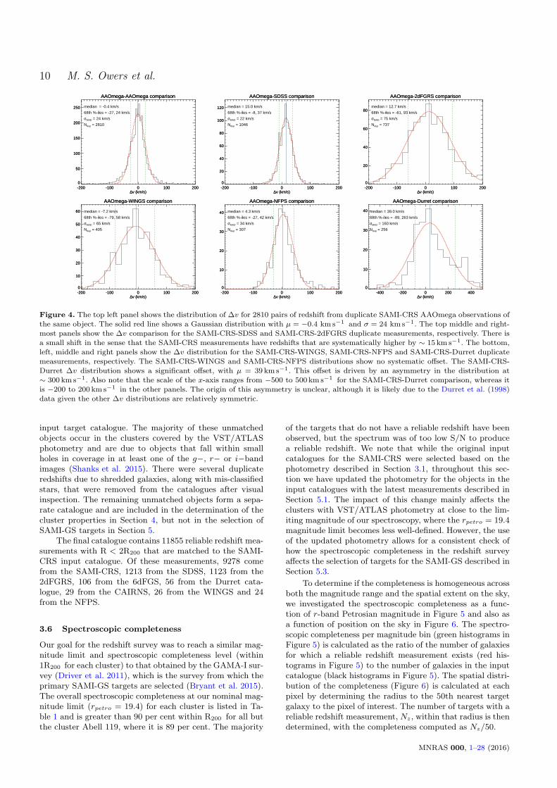
Figure 4. The top left panel shows the distribution of ∆v for 2810 pairs of redshift from duplicate SAMI-CRS AAOmega observations of

the same object. The solid red line shows a Gaussian distribution with µ = −0.4 km s−1 and σ = 24 km s−1. The top middle and right-most panels show the ∆v comparison for the SAMI-CRS-SDSS and SAMI-CRS-2dFGRS duplicate measurements, respectively. There isa small shift in the sense that the SAMI-CRS measurements have redshifts that are systematically higher by ∼ 15 km s−1. The bottom,

left, middle and right panels show the ∆v distribution for the SAMI-CRS-WINGS, SAMI-CRS-NFPS and SAMI-CRS-Durret duplicatemeasurements, respectively. The SAMI-CRS-WINGS and SAMI-CRS-NFPS distributions show no systematic offset. The SAMI-CRS-Durret ∆v distribution shows a significant offset, with µ = 39 km s−1. This offset is driven by an asymmetry in the distribution at∼ 300 km s−1. Also note that the scale of the x-axis ranges from −500 to 500 km s−1 for the SAMI-CRS-Durret comparison, whereas it

is −200 to 200 km s−1 in the other panels. The origin of this asymmetry is unclear, although it is likely due to the Durret et al. (1998)data given the other ∆v distributions are relatively symmetric.

input target catalogue. The majority of these unmatchedobjects occur in the clusters covered by the VST/ATLASphotometry and are due to objects that fall within smallholes in coverage in at least one of the g−, r− or i−bandimages (Shanks et al. 2015). There were several duplicateredshifts due to shredded galaxies, along with mis-classifiedstars, that were removed from the catalogues after visualinspection. The remaining unmatched objects form a sepa-rate catalogue and are included in the determination of thecluster properties in Section 4, but not in the selection ofSAMI-GS targets in Section 5.

The final catalogue contains 11855 reliable redshift mea-surements with R < 2R200 that are matched to the SAMI-CRS input catalogue. Of these measurements, 9278 comefrom the SAMI-CRS, 1213 from the SDSS, 1123 from the2dFGRS, 106 from the 6dFGS, 56 from the Durret cata-logue, 29 from the CAIRNS, 26 from the WINGS and 24from the NFPS.

3.6 Spectroscopic completeness

Our goal for the redshift survey was to reach a similar mag-nitude limit and spectroscopic completeness level (within1R200 for each cluster) to that obtained by the GAMA-I sur-vey (Driver et al. 2011), which is the survey from which theprimary SAMI-GS targets are selected (Bryant et al. 2015).The overall spectroscopic completeness at our nominal mag-nitude limit (rpetro = 19.4) for each cluster is listed in Ta-ble 1 and is greater than 90 per cent within R200 for all butthe cluster Abell 119, where it is 89 per cent. The majority

of the targets that do not have a reliable redshift have beenobserved, but the spectrum was of too low S/N to producea reliable redshift. We note that while the original inputcatalogues for the SAMI-CRS were selected based on thephotometry described in Section 3.1, throughout this sec-tion we have updated the photometry for the objects in theinput catalogues with the latest measurements described inSection 5.1. The impact of this change mainly affects theclusters with VST/ATLAS photometry at close to the lim-iting magnitude of our spectroscopy, where the rpetro = 19.4magnitude limit becomes less well-defined. However, the useof the updated photometry allows for a consistent check ofhow the spectroscopic completeness in the redshift surveyaffects the selection of targets for the SAMI-GS described inSection 5.3.

To determine if the completeness is homogeneous acrossboth the magnitude range and the spatial extent on the sky,we investigated the spectroscopic completeness as a func-tion of r-band Petrosian magnitude in Figure 5 and also asa function of position on the sky in Figure 6. The spectro-scopic completeness per magnitude bin (green histograms inFigure 5) is calculated as the ratio of the number of galaxiesfor which a reliable redshift measurement exists (red his-tograms in Figure 5) to the number of galaxies in the inputcatalogue (black histograms in Figure 5). The spatial distri-bution of the completeness (Figure 6) is calculated at eachpixel by determining the radius to the 50th nearest targetgalaxy to the pixel of interest. The number of targets with areliable redshift measurement, Nz, within that radius is thendetermined, with the completeness computed as Nz/50.

MNRAS 000, 1–28 (2016)


0.0

0.2

0.4

0.6

0.8

1.0

APMCC_0917Peak = 161

Abell_0168Peak = 310


EDCC_0442Peak = 209

0.0

0.2

0.4

0.6

0.8

1.0

13 14 15 16 17 18 19


13 14 15 16 17 18 19


13 14 15 16 17 18 19


13 14 15 16 17 18 19


r-band Magnitude (Petrosian)

Fra

ctio

n

Figure 5. Fractional galaxy numbers and completeness as a function of r-band Petrosian magnitude for galaxies within 2R200. Blackhistogram shows the input target catalogue, the red histogram shows the number of galaxies with reliable redshift measurements, andthe green line shows the spectroscopic completeness as a function of r-band magnitude.

-2

-1

0

1

2

-2 -1 0 1 2

APMCC_0917

-2

-1

0

1

2

-2 -1 0 1 2

Abell_0168

-3

-2

-1

0

1

2

3

-3 -2 -1 0 1 2 3

Abell_3880

-2

-1

0

1

2

-2 -1 0 1 2

EDCC_0442

-2

-1

0

1

2

-2 -1 0 1 2

Abell_4038

-3

-2

-1

0

1

2

3

-3 -2 -1 0 1 2 3

Abell_2399

-4

-2

0

2

4

-4 -2 0 2 4

Abell_0119

-4

-2

0

2

4

-4 -2 0 2 4

Abell_0085

0.4

0.5

0.6

0.7

0.8

0.9

1.0

Spe

ctro

scop

ic C

ompl

eten

ess

X (Mpc)

Y (

Mpc

)

Figure 6. The spatial distribution of the spectroscopic completeness. For each 150 × 150 kpc2 pixel, a radius, R, was defined which

contains 50 galaxies from the input catalogue. The spectroscopic completeness at that pixel is defined as N(< R)z/50. The black dashedcircle shows the R200 radius, and the black solid circle shows the 2R200 radius. The grey contours show the member galaxy isopleths asshown in Figure 10.

Clearly, we do not reach the high level of completenessachieved in the GAMA-I survey (∼ 98%) for all of the clus-ters. In particular, for the clusters A119, APMCC0917 andA4038 the completeness drops below 80% for galaxies fainterthan rpetro = 19. To determine if the lower spectroscopiccompleteness at fainter magnitudes will impact the selec-tion of SAMI-GS targets described in Section 5, we investi-gate the spectroscopic completeness as a function of positionin the colour-magnitude diagram. Since the g- and i-bandmagnitudes are used to determine the stellar mass proxy forSAMI-GS target selection (see Equation 6), we plot the com-pleteness in (g−i) versus i in Figure 7. Overplotted are lines

showing how the i-band magnitude varies with g − i colourfor the stellar mass limits log10(M∗

approx/M⊙) = 8.2, 9.0 and10.0. These are the stellar mass limits used for the mainSAMI-GS primary target selection for galaxies in the red-shift range probed by the clusters (Bryant et al. 2015). The(g−i)-i trends are determined from Equation 6 and using thecluster redshift, zclus. The two clusters A4038 and A119 havelow spectroscopic completeness (< 60%) at the main SAMI-GS limits for their redshifts (log10(M∗

approx/M⊙) = 8.2, 9.0,respectively), particularly for galaxies on the cluster red-sequence (shown as red line in each panel of Figure 7). How-ever, for the reasons outlined in Section 5, we set a lower

MNRAS 000, 1–28 (2016)


limit of log10(M∗approx/M⊙) = 9.5 for the primary cluster

targets when zclus < 0.045. The black lines in Figure 7 showhow the i-band magnitude varies with g − i colour for thestellar mass limits determined for the clusters in Section 5.At these stellar mass limits, the spectroscopic completenessis > 95 per cent for all clusters. Moreover, the depth of thesurvey (at least 3 magnitudes fainter than the knee in thecluster luminosity function) allows for the collection of alarge number of spectroscopically confirmed members evenat the relatively poorer completeness levels reached for A119.The large number of cluster member redshifts will enablethe robust characterisation of the dynamical properties ofthe clusters. We therefore conclude that, despite not quiteachieving our initial goals, the SAMI-CRS is sufficient forour purposes. Importantly, Figure 7 shows that at the stellarmass limits used to define primary targets for the SAMI-GSin Section 5.3, the spectroscopic completeness is very highand will not impact the target selection for the SAMI-GS.

4 CLUSTER MEMBERSHIP AND GLOBALPARAMETERS

In this section, we describe the selection of spectroscopicallyconfirmed cluster members and parameters derived from themember redshifts such as the cluster redshift, velocity dis-persion and mass. These parameters are listed for each clus-ter in Table 1.

4.1 Determination of cluster membership,velocity dispersion and R200

The allocation of cluster membership is a multi-step pro-cess. First, obvious interlopers are rejected as non-membersif they lie further than a projected distance of R = 6 Mpcfrom the cluster centre and have peculiar velocity |vpec| ≥5000 km s−1 where vpec = c(z − zCCG)/(1 + zCCG), zCCG

is the bright central cluster galaxy (CCG) redshift, whichis a good initial approximation of the cluster redshift. Theprojected distances are measured from the R.A. and decl.of the cluster centres listed in Table 1. In the majority ofcases, the selection of the cluster centre is obvious; there isa single bright, CCG for A3880, EDCC 442, A119 and A85which marks the cluster centre. However, for APMCC0917,A4038, A168 and A2399 there are one or more candidatesfor a CCG. In those cases, the coordinates of the bright-est CCG closest to the peak in galaxy surface density (seeSection 4.3) was used for the cluster centre. For the clus-ters A168, APMCC0917 and A2399, the CCG closest to thepeak in the galaxy density distribution was not the bright-est galaxy in the cluster. In fact, for these three clusters thebrightest cluster galaxies were located as far as 800 kpc fromthe defined cluster centre. As we will show in Section 4.3,A168 and A2399 host substructures associated with thesebright galaxies. We note that the centres for A168 and A2399differ from those listed in Bryant et al. (2015).

Following this cut in peculiar velocity and clustercentricdistance, the remaining galaxies are used to obtain an esti-mate of the cluster velocity dispersion, σ200, using the bi-weight scale estimator, which is a robust estimator of scalein the presence of outliers (Beers et al. 1990). The value of

σ200 is determined from those galaxies within the virial ra-dius, which is estimated as R200 = 0.17σ200/H(z) Mpc 11.Since R200 ∝ σ200, the process is iterated until the values ofR200 and σ200 are stable. A second cut in peculiar velocity isthen applied such that those galaxies with |vpec| > 3.5σ200

are removed from the member sample. The galaxies that areremoved by the 3.5σ200 cuts are shown as black open squaresin Figure 8.

The above method of using only velocity infor-mation is sufficient for the identification of obviousnon-members, however, it is not a completely rigorousapproach to interloper rejection (den Hartog & Katgert1996; van Haarlem et al. 1997; Wojtak & Lokas 2007;Wojtak et al. 2007). More robust techniques for identify-ing line-of-sight interlopers utilize the peculiar velocity asa function of cluster-centric-distance. Here, for the secondstep in selecting cluster members we use a slightly modi-fied version of the “shifting-gapper” technique (Fadda et al.1996) which has the advantages of being a fast, model-independent method of interloper rejection. The “shifting-gapper” is applied as follows. Centred at the radius of eachpotential cluster member, an adaptive annular bin contain-ing at least N = 50 other potential cluster members is gen-erated. Within this bin, the galaxies are sorted in order ofincreasing vpec. The velocity difference between successivegalaxies is determined as vgap = vi+1 − vi. Any galaxy thatis separated by a vgap > σ200 from the adjacent galaxyis rejected as a non-member, as are all galaxies with vpeclarger than (or smaller than for negative vpec) the newly de-fined non-member. Galaxies identified as non-members us-ing this method are shown in Figure 8 as black open cir-cles. We note that the choice of σ200 as the maximum al-lowed gap is somewhat arbitrary, although it was found toproduce good results here (see Figure 8), and in other clus-ters (e.g., Zabludoff et al. 1990; Owers et al. 2009a,b, 2011a;Nascimento et al. 2016).

The next step in the procedure involves using theadaptively-smoothed distribution of galaxies in vpec-radiusspace to locate the cluster caustics (Diaferio 1999). The caus-tics trace the escape velocity of the cluster as a function ofcluster-centric radius and, therefore, robustly identify theboundary in vpec−radius space between bona-fide clustermembers and line-of-sight interlopers (e.g., Serra & Diaferio2013; Owers et al. 2013, 2014). Identifying the location ofthe caustics in the projected-phase-space (PPS) diagram re-quires determining an adaptive smoothing kernel that min-imises statistical fluctuations without over-smoothing realstructure in dense regions.

Our procedure for determining such an adaptive kernelfollows the general procedure outlined by Silverman (1986)(see also Pisani (1996) and Diaferio (1999)). Briefly, an ini-tial pilot estimation of the density distribution in PPS is de-termined by smoothing the PPS distribution with a kernel offixed width. The width of this kernel, σsmth, is determined bythe Silverman’s rule of thumb estimate σsmth = AσdistN

−1/6

where N is the number of data points, A = 0.8 (which is 25

11 where R200 is the cluster radius within which the mean densityis 200 times the critical density, where the cluster density distri-bution is assumed to follow that of a single isothermal sphere(Carlberg et al. 1997)

MNRAS 000, 1–28 (2016)


12 14 16 18 200.0

0.5

1.0

1.5

2.0 APMCC_0917

12 14 16 18 200.0

0.5

1.0

1.5

2.0 Abell_0168

12 14 16 18 200.0

0.5

1.0

1.5

2.0 Abell_3880

12 14 16 18 200.0

0.5

1.0

1.5

2.0 EDCC_0442

12 14 16 18 200.0

0.5

1.0

1.5

2.0 Abell_4038

12 14 16 18 200.0

0.5

1.0

1.5

2.0 Abell_2399

12 14 16 18 200.0

0.5

1.0

1.5

2.0 Abell_0119

12 14 16 18 200.0

0.5

1.0

1.5

2.0 Abell_0085

0.4

0.5

0.6

0.7

0.8

0.9

1.0

Spe

ctro

scop

ic C

ompl

eten

ess

iKron (MW extinction corrected)

(g-i)

Figure 7. The spectroscopic completeness as a function of position in (g − i) vs i for galaxies with R < 2R200. The solid red line

shows the position of the cluster red sequence and the dashed red line shows the upper 2σ scatter around the red-sequence. The greenlines show the i-band magnitude as a function of (g − i) colour for stellar mass limits used in the main portion of the SAMI-GS, i.e.,log10(M∗

approx/M⊙) = 8.2, 9.0, and 10 (dotted, dashed and dot-dashed lines, respectively). These trends are determined using Equation 6.The solid black line shows the trend for the stellar mass limit of the cluster of interest; either log10(M∗

approx/M⊙) = 9.5 or 10, depending

on zclus (see Section 5).

percent below the optimal value for a Gaussian kernel, asrecommended by Silverman 1986, to avoid over-smoothingin the presence of multi-modality), and σdist is an estimateof the standard deviation of the distribution. The final valuefor σdist is taken to be the minimum of a number of estima-tors including the standard deviation, median-absolute de-viation, the interquartile range, sigma-clipped, biweight andthe standard deviation estimated when including higher or-der Gauss-Hermite polynomials (as described in Owers et al.2009a; Zabludoff et al. 1993). The estimate for σsmth is de-termined separately for the distributions in the vpec and ra-dial direction; the σdist is determined from the distributionof galaxies with cluster-centric distances less than R200.

The pilot estimate of the density distribution isused to define the local kernel widths σR,vpec =

hR,vpec(γ/fP (R, vpec))1/2, where fP (R, vpec) is the pilot den-

sity at the point of interest, log(γ) = log(fP (R, vpec)), andthe hR,vpec values control the amount of smoothing in thex- and y-directions. The hR,vpec values are determined iter-atively by using least-squares cross validation as describedelsewhere (Silverman 1986; Diaferio 1999). The locally adap-tive smoothing kernels are used to produce the final estimateof the density in PPS, f(R, vpec).

Having adaptively smoothed the PPS distribution, thelocation of the caustics need to be determined. This isachieved by determining the value f(R, vpec) = κ that min-imises (⟨vesc(R200)2⟩−4σ2

200)2 where σ200 is the velocity dis-persion determined within R200 using the biweight estimate,

⟨vesc(R200)2⟩ =

∫ R200

0

A2κ(R)φ(R)dR/

∫ R200

0

φ(R)dR (2)

with φ(R) =∫f(R, v)dv (Diaferio 1999). The value of

Aκ(R) is the location of the caustic amplitude that tracesthe escape velocity as a function of radius for a given κvalue. As described in Serra & Diaferio (2013), due to asym-metries in the velocity component of the f(R, vpec) dis-tribution, a single κ value results in two distinct velocitychoices for Aκ(R), vpos(R) and vneg(R), where in general|vneg(R)| = vpos(R). For the purpose of membership selec-tion, the choice of Aκ(R) is somewhat subjective, but ingeneral the chosen Aκ(R) is the one that falls on the clean-est side of the vpec distribution. For example, for A85 andA4038 the separation between the main cluster and the line-of-sight interlopers is far cleaner on the vneg(R) side of thePPS distribution, and so we set Aκ(R) = |vneg(R)|. Uncer-tainties on the values of A(R) are estimated as described inDiaferio (1999), i.e., δA(R)/A(R) ≃ κ/max(f(R, vpec)). Formember selection, we reject any galaxy at radius R that has|vpec| > A(R) + δA(R) as interlopers (shown as open trian-gles in Figure 8), while any galaxy that was initially rejectedas a non-member during the shifting-gapper selection, buthas |vpec| ≤ A(R) is reinstated as a cluster member. Thisprocess of shift-gapper plus caustics member allocation is it-erated until the number of members within 2R200 becomesstable. At each iteration the cluster redshift, the σ200 andthe R200 are remeasured. The number of spectroscopicallyconfirmed cluster members within R200 and 2R200 is shownin Table 1. In total, there are 1935 and 2899 confirmed mem-bers within R200 and 2R200, respectively.

4.2 Cluster mass measurements

For each cluster the final catalogue of cluster members isused to determine the cluster redshift, velocity dispersion,R200 and M200 listed in Table 1. The virial radius estimate,

MNRAS 000, 1–28 (2016)


0.0 0.5 1.0 1.5 2.0Radius (Mpc)

-4

-2

0

2

4

v pec

(100

0 km

s-1)

APMCC_0917

-0.5 0.5 1.5 2.5 3.5-0.5 0.5 1.5 2.5 3.5

-10

-5

0

5

10

v pec/σ

200

0.0 0.5 1.0 1.5 2.0R/R200

0.0 0.5 1.0 1.5 2.0 2.5Radius (Mpc)

-4

-2

0

2

4

v pec

(100

0 km

s-1)

Abell_0168

-0.5 0.5 1.5 2.5 3.5-0.5 0.5 1.5 2.5 3.5

-5

0

5

v pec/σ

200

0.0 0.5 1.0 1.5 2.0R/R200

0.0 0.5 1.0 1.5 2.0 2.5 3.0Radius (Mpc)

-4

-2

0

2

4

v pec

(100

0 km

s-1)

Abell_3880

0 1 2 3 40 1 2 3 4

-6

-4

-2

0

2

4

6v p

ec/σ

200

0.0 0.5 1.0 1.5 2.0R/R200

0.0 0.5 1.0 1.5 2.0 2.5Radius (Mpc)

-4

-2

0

2

4

v pec

(100

0 km

s-1)

EDCC_0442

-0.5 0.5 1.5 2.5 3.5-0.5 0.5 1.5 2.5 3.5

-5

0

5

v pec/σ

200

0.0 0.5 1.0 1.5 2.0R/R200

0.0 0.5 1.0 1.5 2.0 2.5Radius (Mpc)

-4

-2

0

2

4

v pec

(100

0 km

s-1)

Abell_4038

-0.5 0.5 1.5 2.5 3.5-0.5 0.5 1.5 2.5 3.5

-5

0

5

v pec/σ

200

0.0 0.5 1.0 1.5 2.0R/R200

0.0 0.5 1.0 1.5 2.0 2.5 3.0Radius (Mpc)

-4

-2

0

2

4

v pec

(100

0 km

s-1)

Abell_2399

0 1 2 3 40 1 2 3 4

-6

-4

-2

0

2

4

6

v pec/σ

200

0.0 0.5 1.0 1.5 2.0R/R200

0 1 2 3 4Radius (Mpc)

-4

-2

0

2

4

v pec

(100

0 km

s-1)

Abell_0119

-1 1 3 5 7-1 1 3 5 7

-4

-2

0

2

4

v pec/σ

200

0.0 0.5 1.0 1.5 2.0R/R200

0 1 2 3 4Radius (Mpc)

-4

-2

0

2

4

v pec

(100

0 km

s-1)

Abell_0085

-1 1 3 5 7-1 1 3 5 7

-4

-2

0

2

4

v pec/σ

200

0.0 0.5 1.0 1.5 2.0R/R200

Figure 8. These figures show the phase-space distribution of galaxies within c|(z − zclus)/(1 + zclus)| < 5000 km s−1and R < 2R200.

The galaxies defined as cluster members are shown as filled black circles. The caustics, which define the vesc profile based on the clustermembers, are shown as solid red lines. Non-members have shapes that reflect the step at which they were rejected; open squares showgalaxies rejected because |vpec| > 3.5σ200, open circles show galaxies rejected by the shift-gapper, and open triangles show galaxiesrejected by the caustics. The vertical dashed lines show the r200 radius and the vertical dotted red line shows the radial limit of the

SAMI FOV (0.5 degree radius). The blue horizontal dotted lines show the 3, 5σ200 limits used for the selection of SAMI targets. Thisselection is allowed to be looser than the caustics selection which may change with more data.

MNRAS 000, 1–28 (2016)


R200, and velocity dispersion, σ200, are determined itera-tively as in Section 4.1. The cluster redshift is determinedusing the biweight estimator of location (Beers et al. 1990)for galaxies within 2R200. The mass, M200, is determinedwithin R200 using both the virial and caustic estimators.The virial mass determination follows the same prescriptiondescribed elsewhere (Girardi et al. 1998; Owers et al. 2009a,2013). Briefly, the corrected virial mass is

M(R < R200) = Mvir − C =3π

2

σ2vRPV

G− C (3)

where C ≈ 0.19Mvir is an approximation to the surfacepressure term correcting for cluster mass external to R200

(Girardi et al. 1998) and the projected virial radius is

RPV =N200(N200 − 1)∑N200i=j+1

∑i−1j=1 R

−1ij

(4)

where R−1ij is the projected separation between the ith and

jth galaxies and N200 is the number of galaxies within R200.The uncertainties provided in Table 1 are estimated by prop-agating the uncertainties on σ200 and RPV , which are esti-mated by using jackknife resampling.

The caustic masses are determined from the caustic am-plitudes, A(R), which are estimated from the adaptivelysmoothed PPS described in Section 4.1. However, for themass measurement we use the more conservative criterionA(R) = min((|vneg(R)|, vpos(R)) so as to minimise the im-pact of asymmetry in the velocity distribution due to, e.g.,substructure and interlopers (Diaferio 1999). The causticmass estimator within a radius R is given in Equation 13of Diaferio (1999) and is

M(< R) =Fβ

G

∫ R

0

A2(R)dR (5)

where the Fβ term is a calibration parameter that accountsfor the combined effect of the radial dependence of the grav-itational potential, the mass density and orbital anisotropyprofiles. Diaferio (1999) argued that the combined effect ofthese profiles is a parameter that is a very slowly vary-ing function of radius, and can be estimated as a con-stant. Here, we set Fβ = 0.7, which is the value suggestedby Serra et al. (2011) based on numerical simulations, al-though we note that other authors have suggested lower val-ues are more appropriate (Diaferio 1999; Gifford & Miller2013; Svensmark et al. 2015). This parametrisation, alongwith the assumption of spherical symmetry, are significantsources of systematic uncertainty in the caustic mass mea-surements (Gifford et al. 2013; Svensmark et al. 2015). Thestatistical uncertainties measured on the caustic masses aredetermined from the uncertainty estimate on the position ofthe caustic following the method outlined in Diaferio (1999).The virial masses are systematically larger than the causticmasses, although the 1σ uncertainties generally overlap forany given cluster. Regardless of this offset, the updated massmeasurements presented in Table 1 show that the clustersselected sample the full mass range expected for rich clus-ters.

It is important to note that the mass determina-tions outlined above differ from those used to measurehalo masses for the GAMA portion of the survey (seeRobotham et al. 2011, for details). The halo mass estimatesof Robotham et al. (2011) are virial-like and are calibrated

using halos from simulated mock catalogues. Future anal-yses will use halo mass as an environment metric, so it isimportant to determine the scaling between the SAMI-CRSand GAMA halo masses due to the different mass estima-tors. To determine this, we select groups from the GAMAgroup catalogue (version 8; G3CV08) that have z < 0.2,σ > 300 km s−1 and more than 30 members as defined bythe Friends-of-Friends algorithm in Robotham et al. (2011),returning 56 halos. We use the iteratively defined centroids,the redshifts and the σ values from the G3CV08 as initialinputs, and then determine membership and mass as out-lined above for galaxies within 6 Mpc and vpec ± 3.5σ of thegroup. We compare the virial and caustic masses to thosedetermined by Robotham et al. (2011) after rescaling theGAMA masses by the suggested calibration factor (A=10;Robotham et al. 2011), and also to our assumed cosmology.We find that the GAMA-determined group masses are a fac-tor of 1.37 (1.25) and 1.66 (1.46) larger than the virial andcaustic mass estimates where the numbers in brackets arethe ratios determined for GAMA groups with N200 > 50.This difference is unsurprising since the GAMA masses arecalibrated to simulated halo masses that can differ from theM200 estimates used here (Jiang et al. 2014). We also com-pare the σ measured in G3CV08 to that determined usingthe method presented above, and find that the GAMA σ val-ues are lower by a factor of 0.96. It is recommended that anyfuture analyses using halo masses from both the cluster andGAMA samples should implement these factors, i.e., in addi-tion to scaling to match cosmology, the cluster virial massesshould be multiplied by 1.25 in order to match GAMA halomasses.

4.3 Cluster structure

The cluster mass measurements derived in Section 4.2 maybe impacted by the presence of cluster-cluster merger activ-ity. The virial mass measurements assume a fully virialised,spherically symmetric cluster and the placement of the caus-tic location, κ, that traces the escape velocity profile as de-scribed in Section 4.1 assumes that the mass within R200 isdistributed as an isothermal sphere. These assumptions areviolated where there exists significant dynamical substruc-ture due to cluster merger activity. Moreover, the dynami-cal growth of clusters may produce additional environmentalinfluences on galaxies over and above those encountered ina relaxed system. We therefore investigate the structure ofthe clusters within R200 using three indicators of dynami-cal substructure: a one-dimensional test for structure on thevelocity distribution, a two-dimensional indicator based ongalaxy positions, and a three-dimensional indicator whichuses the combination of position and velocity.

The one-dimensional indicator uses a Gauss-Hermitedecomposition of the velocity distribution to test for de-partures from the Gaussian shape expected of fully viri-alised clusters. The method for this Gauss-Hermite decom-position is described in detail elsewhere (Zabludoff et al.1993; Owers et al. 2009a). This method is sensitive to merg-ers that are occurring on an axis that is highly inclinedto the plane of the sky, which can cause significant skew-ness or kurtosis in the velocity distribution (e.g., as seen inAbell 2744 Owers et al. 2011a). The skewness (the h3 termin the Gauss-Hermite series) and kurtosis (the h4 term in the

MNRAS 000, 1–28 (2016)


Gauss-Hermite series) are measures of asymmetric and sym-metric deviations from a Gaussian shape. The binned veloc-ity distributions (black histograms), along with the Gauss-Hermite reconstructions (red dashed curves), and the best-fitting Gaussian (black curves) for each cluster are shownin Figure 9. The probability that the observed h3 and h4

terms are simply due to random fluctuations in the distri-bution, P[h3,4], is determined as described in Zabludoff et al.(1993). Briefly, we measure the h3 and h4 terms for 10000random Gaussian distributions with the same sample size asthe cluster of interest and using the best-fit mean and dis-persion (listed in the top left of each panel in Figure 9). Thecomparison of the distributions of the simulated h3,4 termswith the observed values shows the frequency with whichrandom fluctuations produce h3,4 values more extreme thanthose measured for the clusters.

In cases where mergers occur close to the plane of thesky, the velocity distribution may not show significant de-partures from a Gaussian shape due to the small line-of-sight velocity difference between the systems (e.g., as seenin Abell 3667; Owers et al. 2009b). In these cases, mergingsubstructures may be identified as localised enhancementsin the projected galaxy density distribution (Geller & Beers1982). These enhancements are best revealed in the adap-tively smoothed isopleths shown as black contours in Fig-ure 10. The adaptive smoothing is performed using the two-step procedure described in Section 4.1.

Tests that use the combination of the position and ve-locity information are the most reliable in detecting sub-structure (Pinkney et al. 1996). Here, we implement theκ-test which uses the Kolmogorov-Smirnov (KS) statisticto determine whether the local velocity distribution to agalaxy of interest is likely to be drawn from the same par-ent distribution as the global cluster velocity distribution(Colless & Dunn 1996). By doing so, the test is able toidentify local departures from the global cluster kinematics,which indicate the presence of dynamical substructure. Here,local is defined to be the

√N nearest neighbours, where N

is the number of cluster members within R200. The resultsof this test are presented in Figure 10 where the size ofthe circles are proportional to −log10PKS , where PKS is theKS-probability that the local and global velocity distribu-tions are drawn from the same parent distribution. Thatis, regions where there are groupings of large circles indi-cate that the kinematics there are different from the globalcluster kinematics. The circles are colour-coded according tothe velocity of the galaxy of interest: red and blue for pos-itive and negative vpec with respect to the cluster, respec-tively. The overall level of substructuring according to theκ-test is calculated by determining κ =

∑Ni=1 −log10PKS .

The significance of κ is determined by remeasuring κ 10,000times and with each iteration removing any correlation be-tween position and velocity by randomly reassigning thegalaxy velocities, while maintaining positions. The value ofP [κsim > κobs] listed at the top left of each panel in Fig-ure 10 gives an indication of the probability that a κobs valueas high as the measured one could occur in the simulationsdue to random fluctuations. Furthermore, circles with large−log10PKS values that rarely occur in the simulations (lessthan 5% of the time) are highlighted in bold.

Combining the results of the tests, it is clear that theclusters A2399 and A85 show significant evidence for the

presence of substructure in all three indicators. The exis-tence of substructure within A85 is well-known from bothX-ray observations (Kempner et al. 2002; Durret et al. 2005;Fogarty et al. 2014; Ichinohe et al. 2015) and previous op-tical observations (Durret et al. 1998; Bravo-Alfaro et al.2009). For A2399, the clustering of large, preferentially red,bubbles ∼ 560 kpc just south of due west of the clus-ter centre is coincident with the brightest cluster galaxywhich has vpec ∼ 1200 km s−1. The X-ray observationsof Bohringer et al. (2007) indicated strong bimodality inA2399, while the X-ray contours shown in Figure 12 ofFogarty et al. (2014) show a plume of X-ray emission ex-tending to the north associated with this structure. Thesepieces of evidence strongly indicate ongoing merger activityin A2399. There is a marginal (P [κsim > κobs] ∼ 0.01) indi-cation of kinematical substructure present in A168, whichis a well-known post-core-passage cluster merger occur-ring with an axis aligned close to the plane of the skybased on its X-ray observations (Hallman & Markevitch2004; Fogarty et al. 2014). Inspection of the κ-test resultsfor A168 in Figure 10 indicate the presence of a kinemat-ical substructure ∼ 800 kpc just East of North that is co-incident with the brightest cluster galaxy, as well as one ofthe X-ray substructures detected in Hallman & Markevitch(2004) and Fogarty et al. (2014). There is a small substruc-ture in A119 that is apparent as a local excess in the pro-jected galaxy density ∼ 1 Mpc to the northeast of the clus-ter centre. This substructure is associated with a brightcluster galaxy and has previously been detected using op-tical data (Kriessler & Beers 1997). The remaining clusters,APMCC0917, A3880, EDCC0442 and A4038 show no strongevidence for substructure.

Pinkney et al. (1996) showed that virial mass estima-tors can overestimate the total cluster mass by as much asa factor of 2 during cluster mergers. They found that theimpact on the measured mass is strongest in the case of lowmass-ratio mergers that are very close to pericentric pas-sage and where the merger axis is within 30 deg of the lineof sight. For those mergers, the high relative velocity of themerging subclusters causes strong bi-modality in the velocitydistribution, leading to an overestimation of the velocity dis-persion and therefore the mass. For less pathological mergerscenarios, they found that masses may be overestimated by∼ 50%, while for mergers with an axis close to the plane ofthe sky (e.g., as in A168), there is minimal impact on themeasured masses. None of the velocity distributions shownin Figure 9 exhibit strong bi-modality, although the clustersA85 and A2399 have h3 ∼ 0.1, indicating asymmetric depar-tures from a single Gaussian shape at the 10% level. How-ever, the velocity dispersions determined for A85 and A2399do not appear to be significantly affected by this asymmetry;compare the dispersion measurements in Table 1 with thosein the upper left corner of Figure 9. In principle, the causticmass measurements should be less-affected by substructure(with the caveat that the velocity dispersion is used in deter-mining where to place the caustics) so it is reassuring thatthe caustics and virial mass estimators for A85 and A2399are not significantly different. We conclude that the clusterswith substructure, particularly A2399 and A85, may havetheir masses overestimated by up to ∼ 50%, although theyare unlikely to be overestimated by the factor of 2 seen inmore extreme situations.

MNRAS 000, 1–28 (2016)


APMCC_0917 (Radius < 1190kpc)

-2000 -1000 0 1000 2000vpec (km s-1)

0

5

10

15

20

25

N

APMCC_0917 (Radius < 1190kpc)

-2000 -1000 0 1000 2000vpec (km s-1)

0

5

10

15

20

25

N

V=-20 km/sS=446 km/sh3=0.032, P[h3]=0.66h4=0.039, P[h4]=0.61

Abell_0168 (Radius < 1324kpc)

-2000 -1000 0 1000 2000vpec (km s-1)

0

10

20

30

40

N


-2000 -1000 0 1000 2000vpec (km s-1)

0

10

20

30

40

N

V=42 km/sS=544 km/sh3=0.055, P[h3]=0.27h4=0.017, P[h4]=0.72


-2000 -1000 0 1000 2000vpec (km s-1)

0

10

20

30

40

N


-2000 -1000 0 1000 2000vpec (km s-1)

0

10

20

30

40

N

V=76 km/sS=570 km/sh3=-0.064, P[h3]=0.23h4=0.117, P[h4]=0.03

EDCC_0442 (Radius < 1409kpc)

-2000 -1000 0 1000 2000vpec (km s-1)

0

5

10

15

20

25

30

35

N

EDCC_0442 (Radius < 1409kpc)

-2000 -1000 0 1000 2000vpec (km s-1)

0

5

10

15

20

25

30

35

N

V=-5 km/sS=590 km/sh3=0.059, P[h3]=0.32h4=-0.036, P[h4]=0.50


-2000 -1000 0 1000 2000vpec (km s-1)

0

10

20

30

40

N


-2000 -1000 0 1000 2000vpec (km s-1)

0

10

20

30

40

N

V=101 km/sS=656 km/sh3=-0.009, P[h3]=0.87h4=-0.099, P[h4]=0.02


-2000 -1000 0 1000 2000vpec (km s-1)

0

10

20

30

40

50

N


-2000 -1000 0 1000 2000vpec (km s-1)

0

10

20

30

40

50

N

V=-116 km/sS=699 km/sh3=0.131, P[h3]=0.00h4=-0.001, P[h4]=0.95


-2000 -1000 0 1000 2000vpec (km s-1)

0

20

40

60

N


-2000 -1000 0 1000 2000vpec (km s-1)

0

20

40

60

N

V=48 km/sS=809 km/sh3=-0.052, P[h3]=0.14h4=0.038, P[h4]=0.28


-2000 -1000 0 1000 2000vpec (km s-1)

0

20

40

60

80

100

N


-2000 -1000 0 1000 2000vpec (km s-1)

0

20

40

60

80

100

N

V=134 km/sS=955 km/sh3=-0.106, P[h3]=0.00h4=0.055, P[h4]=0.05

Figure 9. The histograms show the velocity distributions for cluster members within R200. The bin size is determined as 3S/(N)(1/3)

where N is the number of galaxies within R200. The solid black line shows the best-fitting Gaussian, while the dashed red line shows theGauss-Hermite reconstruction of the velocity distribution. In each panel, the best-fitting Gaussian parameters, the Gauss-Hermite termsh3 and h4, representing the asymmetric and symmetric deviations from a Gaussian shape, and their associated level of significance aregiven in the upper left corner.MNRAS 000, 1–28 (2016)


APMCC_0917

-1.0 -0.5 0.0 0.5 1.0X / Mpc

-1.0

-0.5

0.0

0.5

1.0

Y /

Mpc

-2.25 -1.75 -1.25 -0.75 -0.25 0.25 0.75 1.25 1.75 2.25

-2.25

-1.75

-1.25

-0.75

-0.25

0.25

0.75

1.25

1.75

2.25

kobs-statistic = 39P[ksim > kobs] = 0.04

Abell_0168

-1.0 -0.5 0.0 0.5 1.0X / Mpc

-1.0

-0.5

0.0

0.5

1.0

Y /

Mpc

-2.25 -1.75 -1.25 -0.75 -0.25 0.25 0.75 1.25 1.75 2.25

-2.25

-1.75

-1.25

-0.75

-0.25

0.25

0.75

1.25

1.75

2.25


Abell_3880

-1.5 -1.0 -0.5 0.0 0.5 1.0 1.5X / Mpc

-1.5

-1.0

-0.5

0.0

0.5

1.0

1.5

Y /

Mpc

-2.25 -1.75 -1.25 -0.75 -0.25 0.25 0.75 1.25 1.75 2.25

-2.25

-1.75

-1.25

-0.75

-0.25

0.25

0.75

1.25

1.75

2.25


EDCC_0442

-1.0 -0.5 0.0 0.5 1.0X / Mpc

-1.0

-0.5

0.0

0.5

1.0

Y /

Mpc

-2.25 -1.75 -1.25 -0.75 -0.25 0.25 0.75 1.25 1.75 2.25

-2.25

-1.75

-1.25

-0.75

-0.25

0.25

0.75

1.25

1.75

2.25


Figure 10. In each panel, the black contours show the galaxy isopleths derived from the adaptively smoothed galaxy distribution. Thecircles centred at the position of each member galaxy show the results of the κ-test. The radius of the each circle is proportional to−log10PKS , where PKS is the probability that the local and global velocity distributions are drawn from the same parent distribution.

The circles are coloured blue or red for galaxies with positive and negative vpec, respectively. Clusterings of large circles indicate thatthe local velocity distribution is different from the global. Bold circles highlight those galaxies where only 5% of simulated −log10PKS

values are larger than the observed values. The observed κ-values, and the probability that a value larger than this one occurs in the

randomly shuffled simulations are given in the top left of each panel.

5 SAMI TARGET SELECTION

Having described the SAMI-CRS and the global clusterproperties, we now use those results as input for selectingthe cluster targets for the SAMI-GS. In this section, we firstdescribe our improved procedure for measuring aperture-and PSF-matched photometry, and verify the photometricprecision and accuracy using internal and external measure-ments. We then describe the selection of cluster targets forthe SAMI-GS.

5.1 Updated Photometry

The SAMI-GS target selection is outlined in Bryant et al.(2015). Briefly, the selection used the combination of red-shift and a stellar mass proxy that is derived from the em-pirical relationship between the stellar mass-to-i-band ratioand (g − i) colour defined by Taylor et al. (2011). The stel-lar mass proxy requires an accurate determination of both(g − i) colour and total i-band magnitude. To that end, weproduce new photometric catalogues for the SAMI clusterswhere a more careful matching of aperture and image-PSF

MNRAS 000, 1–28 (2016)


Abell_4038

-1.0 -0.5 0.0 0.5 1.0X / Mpc

-1.0

-0.5

0.0

0.5

1.0

Y /

Mpc

-2.25 -1.75 -1.25 -0.75 -0.25 0.25 0.75 1.25 1.75 2.25

-2.25

-1.75

-1.25

-0.75

-0.25

0.25

0.75

1.25

1.75

2.25


Abell_2399

-1.5 -1.0 -0.5 0.0 0.5 1.0 1.5X / Mpc

-1.5

-1.0

-0.5

0.0

0.5

1.0

1.5

Y /

Mpc

-2.25 -1.75 -1.25 -0.75 -0.25 0.25 0.75 1.25 1.75 2.25

-2.25

-1.75

-1.25

-0.75

-0.25

0.25

0.75

1.25

1.75

2.25


Abell_0119

-2 -1 0 1 2X / Mpc

-2

-1

0

1

2

Y /

Mpc

-2.22 -1.67 -1.11 -0.56 0.00 0.56 1.11 1.67 2.22 2.78

-2.22

-1.67

-1.11

-0.56

0.00

0.56

1.11

1.67

2.22

2.78


Abell_0085

-2 -1 0 1 2X / Mpc

-2

-1

0

1

2

Y /

Mpc

-4.5 -3.5 -2.5 -1.5 -0.5 0.5 1.5 2.5 3.5 4.5

-4.5

-3.5

-2.5

-1.5

-0.5

0.5

1.5

2.5

3.5

4.5


Figure 10 – continued

homogenisation has been achieved. The process is outlinedbelow.

5.1.1 SDSS clusters

For the four clusters that lie within the SDSS footprint(Abell 85, Abell 2399, Abell 168 and Abell 119) the photom-etry has been re-measured using the IOTA software, whichwas used to measure aperture-matched photometry for theGAMA survey (Hill et al. 2011; Driver et al. 2016). Priorto running the IOTA software, all image frames in the ugrizbands and within a 4 deg×4 deg region surrounding the clus-ter centres were retrieved from the SDSS DR10 database.Each frame was convolved to a common PSF (FWHM=2′′)and renormalised to a common zero-point (ZP) (Hill et al.

2011; Driver et al. 2016). For each of the ugriz bands, theconvolved, renormalised frames were then combined usingthe SWarp software (Bertin et al. 2002; Bertin 2010). Thephotometry for each of the combined ugriz images was mea-sured using the SExtractor software (Bertin & Arnouts 1996,2010) in dual-image mode with the r-band image used fordetection. This method is consistent with that used to mea-sure the photometry in the GAMA portion of the SAMI-GS.

5.1.2 VST/ATLAS clusters

The images produced by CASU for the VST/ATLAS surveyare not suitable for measuring accurate photometry. The pri-mary reason behind this is that the illumination correction isnot applied to the images themselves, but rather to the pho-

MNRAS 000, 1–28 (2016)


tometric catalogues in a post-processing step (Shanks et al.2015). This illumination correction accounts for the ∼0.2mag centre-to-edge gradient due to the impact of scat-tered light on the flat-fielding. To overcome this issue, rawVST/ATLAS data in the gri-bands were retrieved from theESO archive and reduced using the Astro-WISE optical im-age reduction pipeline (McFarland et al. 2013) for the clus-ters Abell 3880, EDCC 0442, the Abell 4038/APMCC0917region and also for the partially-covered Abell 85 region(which will be used for quality control tests in Section 5.1.3).The reduction follows the general procedure outlined for theKilo-Degree Survey data releases described in de Jong et al.(2015), with several modifications that are required to ac-count for the two-pointing dither pattern (as opposed to theKiDs 5-pointing dither pattern) and the brighter magnitudelimits of the VST/ATLAS survey (which affects the astro-metric calibration). The reduction produces calibrated coad-ded images that have the illumination correction applied andhave photometric zero-points tied to the ESO nightly stan-dards.

Because there can be significant variation in thenight-to-night photometric zero-points, we measure theaperture- and PSF-matched photometry separately for each1 deg×1 deg gri coadded image and correct the photome-try on a tile-by-tile basis as follows. On each full resolu-tion gri coadded image, SExtractor is used to detect sourcesand extract photometric parameters. Stellar magnitudes aremeasured using 6.4′′ diameter apertures and are correctedfor PSF-dependent aperture losses using a curve-of-growth(COG) correction (Howell 1989). The COG correction is de-termined from ∼ 1000 stars in each tile with magnitudesin the range 15 < gri < 20. For each of these stars, thedifferential magnitude profile is measured through a seriesof concentric apertures. At the radius of each aperture, themedian value of the ∼ 1000 differential magnitude values isused to determine the median differential magnitude profile.The aperture correction is determined by integrating themedian differential profile out to a 15′′ diameter aperture.Following the method described in Section 3.1.1, for eachtile the bright, non-saturated stars are cross-matched withAPASS stars. The median difference between the APASSand COG-corrected total magnitudes are used to derive acorrection which ties each gri-band tile to the APASS pho-tometry. The corrections are generally of the order 0.05 mag,although in some cases were as high as 0.15 mag. A furthersmall correction is then applied to place the gri photometryonto the SDSS system using the colour transforms derivedby Shanks et al. (2015).

The aperture- and PSF-matched photometry is mea-sured in a similar manner to that described for the SDSSdata (Section 5.1.1). Since the VST/ATLAS imaging hashigher image quality than the SDSS (Shanks et al. 2015),we convolved each gri-band tile to a common 1.5′′ FWHM.For the convolution, it is assumed that the seeing mea-surement provided within the tile header, FWHMseeing, isaccurate and that the PSF has a Gaussian shape. Theamount by which the image is convolved is FWHMconvolve =√

1.52 − FWHMseeing2. We run SExtractor in dual-image

mode using the r-band image as the detection image. Foreach tile the separate photometric catalogues for the fullresolution and convolved gri-bands are matched to the full-resolution r-band catalogue. Finally, the photometric cat-

alogues for the separate tiles are concatenated. Duplicatedmeasurements due to the 2′ overlap between adjacent tilesare accounted for by keeping the photometric measurementwith the highest quality as determined based on the SExtrac-tor flags. We make use of these duplicated measurements of15 < r < 20 stars in the overlap regions to test the tile-to-tile variations in the photometric calibration. For each clus-ter, we find that the median difference in the distribution ofgri-magnitudes is always smaller than ±0.016 mag and thedispersion in the distribution is smaller than 0.05 mag. Thisinternal comparison indicates that the VST/ATLAS pho-tometry has good precision, with low tile-to-tile variation.

5.1.3 Comparison of SDSS and VST/ATLAS photometry

We conducted a number of tests to ensure there are no sys-tematic offsets between the SDSS and VST/ATLAS pho-tometry which may bias the target selection. First, wemake use of the well-known stellar locus produced by main-sequence stars in colour-colour space. In Figure 11, the fourpanels show the galactic-extinction-corrected (g − r) ver-sus (r − i) diagrams for stars with COG-corrected aperturemagnitudes 15 < r < 20. Overplotted as thick black linesare the median stellar locus trends determined from high-quality SDSS stars presented by Covey et al. (2007). For allpanels, the median SDSS stellar locus tracks very closelywith the peak in the number density distribution. This isrevealed in more detail in Figure 12 where the residuals in(g − i)VST/ATLAS colours after subtracting the Covey et al.(2007) stellar loci for the SDSS stars are plotted as a func-tion of VST/ATLAS colour. The difference is consistent withzero, with scatter generally less than 0.1mag. This indicatesthat there are no systematic offset in the colours measuredfor the VST/ATLAS stars when compared with the SDSSmeasurements.

The second test utilises the fact that A85 cluster is cov-ered by the SDSS photometry and also partially coveredby the VST/ATLAS survey. We use this overlap to directlyassess the total magnitude estimates for the galaxy pho-tometry from VST/ATLAS by comparing with those de-termined by the IOTA software in Section 5.1.1, as well asthe stellar mass proxies determined in Section 5.2. Thesecomparisons are shown in Figure 13 where it can be seenthat the differences in gri-band Kron-like measurementsfrom the aperture and PSF-matched catalogues differ byonly small amounts, typically by less than 0.015mag. The1σ scatter around the offsets is small (∼ 0.06 − 0.08 mag),and increases at fainter magnitudes as shown by the dashedred lines in Figure 13. The random uncertainties in thegri-bands for the VST/ATLAS (SDSS) measurements are∆(g, r, i) = (0.003 − 0.04, 0.002 − 0.03, 0.003 − 0.03) mag(0.006−0.05, 0.003−0.05, 0.005−0.08 mag) over the magni-tude ranges shown in Figure 13. For magnitudes fainter than∼ 17.5, the quadrature sum of the VST/ATLAS and SDSSuncertainties, shown as green bars in Figure 13, account forthe majority of the scatter in the magnitude differences. Forbrighter magnitudes, the random uncertainties are arounda factor of 5-10 too small to account for the scatter in themagnitude differences. At these brighter magnitudes, othersources of uncertainty such as differences in aperture defi-nition, background subtraction and zeropoint offsets domi-nate over the random uncertainties. Taking the quadrature

MNRAS 000, 1–28 (2016)


Abell_4038

-0.5 0.0 0.5 1.0 1.5 2.0g-r

-0.5

0.0

0.5

1.0

1.5

2.0

r-i

1 10 100

Abell_3880

-0.5 0.0 0.5 1.0 1.5 2.0g-r

-0.5

0.0

0.5

1.0

1.5

2.0

r-i

1 10 100

EDCC_0442

-0.5 0.0 0.5 1.0 1.5 2.0g-r

-0.5

0.0

0.5

1.0

1.5

2.0

r-i

1 10 100

Abell_0085

-0.5 0.0 0.5 1.0 1.5 2.0g-r

-0.5

0.0

0.5

1.0

1.5

2.0

r-i

1 10 100

Figure 11. Extinction-corrected (gr) vs (ri) colour-colour diagrams for stars selected from VST/ATLAS photometry for the clusters

A4038, A3880, A85 and EDCC0442. The stars have COG-corrected aperture magnitudes in the range 15 < r < 20. The colour scalegives the number of stars in each bin, as indicated by the colour bar shown in the upper left corner of each panel. in the upper left cornershow the The black line overlaid on these diagrams shows the median stellar locus of high-quality SDSS stars from Covey et al. (2007).

These plots confirm that there are no large systematic offsets in colours measured with the VST/ATLAS photometry when comparedwith the SDSS.

difference between the 1σ scatter around the offsets andthe random uncertainties indicates that these other sourcesof uncertainties amount to 0.03 − 0.04 mag. Shanks et al.(2015) find that the uncertainty on the zeropoints for theVST/ATLAS survey are of order 0.01− 0.02 mag when tiedto APASS photometry. This indicates that aperture def-inition, background subtraction and other systematic un-certainties contribute of the order 0.02 − 0.04 mag to theoverall uncertainty budget. There is a marginal trend inthe i-band difference in the sense that the difference inmagnitude increases to 0.03 − 0.04mag for i < 18 withthe VST/ATLAS measurements being brighter. The stel-lar mass determinations differ by only 0.04 dex, in the sensethat the VST/ATLAS measurements are higher than theSDSS/IOTA measurements, and have a small scatter (∼0.06 dex). These comparisons indicate that the systematicdifferences between the SDSS/IOTA and the VST/ATLASphotometry are small and will not significantly bias the se-lection of SAMI targets.

5.2 Stellar mass estimates

The spectroscopically confirmed SAMI targets from Sec-tion 3.5 are matched to the aperture-matched photomet-ric catalogues using a 3′′ matching radius. Stellar massesare then estimated using the empirical proxy described byTaylor et al. (2011) which uses the fact that the (g−i) colourin the galaxy frame of reference strongly correlates with themass-to-i-band-light ratio, M∗/Li. The stellar mass proxy,M∗

approx, is the same as that used in Bryant et al. (2015) forthe GAMA portion of the SAMI-GS selection. The relation-ship with observed g- and i-band magnitudes is

M∗approx = −0.4i + 2log10(DL) − log10(1 + z)+

(1.2177 − 0.5893z) + (0.7106 − 0.1467z)(g − i)(6)

where the first three terms effectively transform the ob-served, extinction-corrected i-band magnitude into an ab-solute magnitude, while the final two terms account for theredshift evolution of the correlation due to the effects ofthe k-correction on the observed colour. Here, (DL) is theluminosity distance (for our assumed cosmology) and it isdetermined using the cluster redshift, which minimises theimpact of the peculiar velocity due to the cluster velocity

MNRAS 000, 1–28 (2016)


Abell_4038

0 1 2 3 4(g-i)VST/ATLAS

-0.4

-0.2

0.0

0.2

0.4

(g-i)

VS

T/A

TLA

S -

(g-

i) SD

SS

1 10 100

Mean = -0.01Sigma = 0.10

Abell_3880


-0.4

-0.2

0.0

0.2

0.4

(g-i)

VS

T/A

TLA

S -

(g-

i) SD

SS

1 10 100

Mean = -0.01Sigma = 0.10

EDCC_0442


-0.4

-0.2

0.0

0.2

0.4

(g-i)

VS

T/A

TLA

S -

(g-

i) SD

SS

1 10

Mean = 0.00Sigma = 0.10

Abell_0085


-0.4

-0.2

0.0

0.2

0.4(g

-i)V

ST

/AT

LAS -

(g-

i) SD

SS

1 10 100

Mean = 0.00Sigma = 0.10

Figure 12. The residual offset in (g − i)VST/ATLAS colour after subtracting the Covey et al. (2007)-defined stellar locus shown inFigure 11 as a function of colour. The colour scale gives the number of stars in each bin, as indicated by the colour bar shown in theupper left corner of each panel. The black dashed lines show the median and 68th percentiles as a function of (g − i)VST/ATLAS colour.There are only very small offsets, consistent with zero, as a function of colour and the dispersion is generally less than 0.1 indicating that

the VST/ATLAS-derived colours are not systematically different from those derived from SDSS photometry. The vertical dot-dashedline shows the upper limit for the (g − i)VST/ATLAS colour of the cluster red-sequence.

dispersion on the M∗approx estimate. The three terms that in-

volve z all correct for the impact of redshift on the observedmagnitude/colour with respect to the intrinsic value and,therefore, use the galaxy redshift. The g- and i-band are theaperture-matched magnitudes determined in Section 5.1 andare corrected for Galactic extinction using the Schlegel et al.(1998) dust maps. This empirical approximation producesvery precise stellar mass estimates when compared with fullspectral energy distribution fitting, with a 1σ error of only0.1 dex (Taylor et al. 2011).

5.3 Cluster target selection for the SAMI-GS

The primary SAMI-GS targets in the GAMA regions are se-lected from a series of redshift bins with an increasing stellarmass limit in higher redshift bins (Bryant et al. 2015). Thisstrategy was developed to cover a relatively broad stellarmass range as required for the science drivers for the survey,to match the target density to the SAMI instrument’s mul-tiplexing capabilities (∼ 15 targets per square degree), andto reach a completeness level of ∼ 90% within the time al-located to the survey. A similar strategy is employed for the

cluster galaxies, however, there are several additional con-straints that must be considered. First, at the cluster red-shifts, the limiting stellar mass used in the GAMA SAMI-GSregions produce a target density that is much higher thanthe ∼ 15 targets per square degree and will require manyrevisits to achieve a 90% completeness limit for the eightclusters. Second, while the low mass M∗ < 109.5 M⊙ galaxypopulation in the lower-density GAMA regions is primarilycomposed of blue, star-forming galaxies with emission lines(Taylor et al. 2015), the low-redshift cluster population atM∗ < 109.5 M⊙ is dominated by red-sequence galaxies (seetop left panel in Figure 14). These lower mass, red-sequencegalaxies have small projected sizes and are faint; they haverpetro > 19.0 for the clusters with zclus > 0.04. These galax-ies are unlikely to produce high S/N SAMI data with a usefulfraction of independently resolved spatial elements. Further-more, as outlined in Section 3.6, the SAMI-CRS begins tosuffer from spectroscopic incompleteness in several clustersfor these low masses (see Figure 7). Third, the projectedsizes of the clusters are large on the sky; the R200 values arecomparable to the SAMI FOV (compare the vertical dashedand red lines in Figure 8). Therefore, for a galaxy to be con-

MNRAS 000, 1–28 (2016)


Abell_0085

14 15 16 17 18 19 20g (SDSS/IOTA)

-0.4

-0.2

0.0

0.2

0.4

g (S

DS

S/IO

TA

) -

g (V

ST

/AT

LAS

)

Mean = -0.015Sigma = 0.069

Abell_0085

14 15 16 17 18 19 20r (SDSS/IOTA)

-0.4

-0.2

0.0

0.2

0.4

r (S

DS

S/IO

TA

) -

r (V

ST

/AT

LAS

)

Mean = -0.011Sigma = 0.064

Abell_0085

14 15 16 17 18 19 20i (SDSS/IOTA)

-0.4

-0.2

0.0

0.2

0.4

i (S

DS

S/IO

TA

) -

i (V

ST

/AT

LAS

)

Mean = 0.012Sigma = 0.079

Abell_0085

8.5 9.0 9.5 10.0 10.5 11.0 11.5 12.0M* (SDSS/IOTA)

-0.4

-0.2

0.0

0.2

0.4M

* (S

DS

S/IO

TA

) -

M* (

VS

T/A

TLA

S)

Mean = -0.036Sigma = 0.056

Figure 13. The comparison between gri magnitudes and stellar mass estimates for galaxies that had both SDSS/IOTA and VST/ATLASphotometry. The top left, top right and bottom left plots show the distribution of SDSS/IOTA-VST/ATLAS differences for the g, r and i-bands, respectively, plotted against the VST/ATLAS measurement. The bottom right panel shows the difference in the M∗

approx estimates

determined using Equation 6. The red solid and dashed lines in each plot show the median and scatter (as measured by the medianabsolute deviation) as a function of g, r and i-band magnitude, as well as M∗

approx. Only small differences exist between SDSS/IOTAand VST/ATLAS-derived quantities. The green bars in the top left, top right and bottom left panels show the quadrature sum of themedian uncertainty on the VST/ATLAS and SDSS measurements in each bin (centred on the median difference in that bin). For bright

magnitudes, the quadrature sum of the uncertainties does not account for the scatter in the differences, indicating that systematicsdominate there.

sidered as a primary target candidate, it must satisfy thefollowing criteria based on clustercentric distance, peculiarvelocity and stellar mass:

• |vpec| < 3.5σ200 km s−1 & R <R200with vpec measuredwith respect to zclus,

• for zclus < 0.045: M∗approx > 109.5 M⊙,

• for 0.045 < zclus < 0.06: M∗approx > 1010 M⊙.

Table 3 lists the number of primary targets based onthese criteria for each cluster. The cut in vpec is shown asa blue dashed line in Figure 8 and is less conservative thanthe velocity cut used to allocate cluster membership as de-scribed in Section 4.1. This less-conservative cut allows forthe uncertainty in allocating cluster membership that, de-spite our best efforts, may be biased against extreme casessuch as high-velocity infalling galaxies. In addition to theprimry targets, we include a number of filler targets for caseswhere twelve primary targets cannot be allocated on a platedue to, e.g., targets being closer than the collision radius of

the SAMI hexabundles (228′′). We define two types of fillertargets; blue filler and large-radius filler targets. The fillersmust meet the following criteria:

• Blue filler: M∗lim−0.5 < M∗

approx < M∗lim & (g−i)kcorr <

0.9 & R <R200.• Large radius filler: M∗

approx > M∗lim & R >R200.

The first selection criterion allows for blue galaxies whichare 0.5 dex less massive than our primary target selec-tion limits to be included, thereby increasing the targetdensity. Here, (g − i)kcorr is the k-corrected colour wherethe k-corrections are determined using the calc kcor code12

from Chilingarian et al. (2010). The second criterion al-lows for objects at slightly larger clustercentric distancewhich become necessary when the tiling software describedin Bryant et al. (2015) selects a plate centre that is offsetfrom the cluster centre by large enough that part of the

12 http://kcor.sai.msu.ru/getthecode/

MNRAS 000, 1–28 (2016)


Figure 14. The k-corrected (g − i) colours versuslog10(M∗

approx/M⊙) for the different SAMI target priori-

ties. The primary targets are shown as red circles and bluefillers as blue circles. Large-radius-fillers are omitted for clarity.The black crosses show the distribution of all spectroscopicallyconfirmed members. The green line shows the best fitting linear

relation to the red-sequence for the primary SAMI-GS clustertargets. The dashed green line shows the dividing line used toseparate red-sequence and blue-cloud galaxies. It is defined asbeing 1.6σRS below the best fitting line, where σRS is the scatter

in the red-sequence around the best fit.

plate area lies beyond R200. The targets are visually in-spected and classified based on the criteria outlined in Ta-ble 5 of Bryant et al. (2015). The number of primary, blue-and large-radius-filler targets per cluster are outlined in Ta-ble 3. The top left panel of Figure 14 shows the colour-massdiagram where primary targets are shown as red circles, bluefillers as blue circles, and non-SAMI-targeted members asblack crosses.

6 SURVEY PROGRESS AND COMPLETENESS

As for the GAMA portion of the SAMI-GS, the aim forthe cluster regions is to reach 90% completeness for the pri-mary targets. However, the input catalogues for the SAMI-GS cluster targets were not finalised in the early stages ofthe survey for two reasons. First, the SAMI-CRS observa-tions were performed after the first cluster SAMI-GS runin September 2013. Second, improvements continued to bemade to the VST/ATLAS photometry during the first twoyears of the survey. The impact of this was twofold. Ini-tially, redshifts and therefore confirmed cluster membershipwas only available for bright, high stellar mass galaxies. Thismeant that only those galaxies could be targeted for theSAMI-GS in the first round of observations. Second, theuncertain photometry meant that a hard cut at the lowerlimits in stellar mass outlined in Section 5.3 was not possi-ble. To mitigate the impact of this, the priorities for targetsin the first two years of the survey were adjusted so thathigher stellar mass objects were preferentially selected forobserving. The combination of the early incomplete redshiftinformation and later the uncertain photometry meant thatselection of targets for SAMI-GS observation were biased to

higher mass objects in the early phases of the survey. Thismay introduce significant biases into the final catalogue ifcare is not taken to track the completeness as a function ofvarious parameters.

We check for potential biases in Figure 15 where we ex-plore the distribution, NP, and survey completeness, Fobs,for primary targets as a function of log10(M∗

approx/M⊙) (toppanel), clustercentric distance (middle panel) and galaxy el-lipticity (bottom panel; as measured by SExtractor duringthe photometric measurements outline in Section 5.1). Thecompleteness is defined as the ratio of observed-to-total pri-mary target galaxies at the end of semester 2015B. Thecompleteness of primary targets for each cluster is listedin Table 3. We also explore the completeness as a functionof log10(M∗

approx/M⊙) for primary SAMI-GS targets splitin to red sequence and blue cloud galaxies based on their(g− i) colour. The boundary for separating the red sequenceand blue cloud galaxies is shown as a dashed green line inFigure 14, and is defined as being 1.6σRS below the best-fitting line to the red sequence galaxies (using the methodoutlined in Section 3.2). Figure 15 shows that the obser-vations to date are indeed biased towards galaxies withhigher log10(M∗

approx/M⊙) with Fobs rising from 43% atlog10(M∗

approx/M⊙) = 9.5 to 85% at log10(M∗approx/M⊙) =

11.5. A similar rising trend is seen for both the red sequenceand blue cloud galaxies. The Fobs trends with ellipticityis relatively flatter, while the trend with R/R200 indicateshigher completeness levels closer to the cluster centres. Thesurvey will continue until at least 2018 and by completionwe aim to reach the Fobs = 90% in each log10(M∗

approx/M⊙)and R/R200 bin.

7 SUMMARY

We have presented the selection and characterisation of eightclusters that are included in the SAMI-GS in addition to theGAMA regions. These additional regions allow the SAMI-GS to probe the full range of galaxy environments, fromthe low density field and groups to the high density clustercores. In Section 3, we provide details of a redshift surveyperformed for each of the eight clusters, the SAMI-CRS. InSection 4, we use the data from the SAMI-CRS to charac-terise a number of cluster properties. The main results forSections 3 and 4 are:

• We have obtained very high spectroscopic completeness(always ≥ 85%, 94% on average) out to large clustercentricdistances (R = 2R200) and to a limiting r-band magnituder = 19.4. This allows for a large number of spectroscopicallyconfirmed cluster members, ranging from 119−772 memberswithin 2R200.

• The large number of cluster members allow very goodmeasures of velocity dispersion, which lie in the range 492−1002 km s−1, and virial mass measurements, which are in therange 14.24 ≤ log(M200/M⊙)≤ 15.19.

• We use the positions and velocities of the confirmedcluster members to investigate the structure of the clusters.The clusters APMCC0917, EDCC0442, A3880, and A4038do not show strong evidence for the existence of substruc-ture. The clusters A168 and A119 show marginal evidencefor substructure while A85 and A2399 both show significantevidence for the existence of multiple substructures.

MNRAS 000, 1–28 (2016)


Table 3. Primary targets selected for the cluster portion of the SAMI-GS. Also listed are blue filler and large radius filler targets, alongwith the number of targets observed to date (as of 2015B). The final column lists the completeness of the primary targets observed as

of semester 2015B.

Cluster zclus Primary Blue R >R200 Observed CompletenessFiller Filler to date percent

APMCC 917 0.0509 29 9 15 22/2/3 76

Abell 168 0.0449 113 17 98 52/0/8 46Abell 4038 0.0293 111 10 143 87/1/8 78EDCC 442 0.0498 50 10 40 41/3/3 82

Abell 3880 0.0578 56 11 93 31/0/4 55Abell 2399 0.0580 94 10 78 70/1/9 75Abell 119 0.0442 259 23 220 107/0/0 41Abell 85 0.0549 171 20 59 82/0/0 48

Total – 883 110 746 492/7/35 56

In Section 5, we describe the target selection for thecluster portion of the SAMI-GS. We detail our procedurefor measuring aperture- and PSF-matched photometry onboth the SDSS and the VST/ATLAS images. The results ofSection 5 can be summarised as follows:

• We confirm the veracity of our VST/ATLAS photome-try by both comparing the duplicated measurements of starsin the overlap regions of the different images. We find thatthe median difference in the duplicated gri measurements isalways less than 0.016 mag, with dispersion ∼ 0.05.

• We compare the stellar locus of our VST/ATLAS pho-tometry to the median SDSS stellar locus of Covey et al.(2007). We find differences consistent with zero and with0.1dex dispersion, indicating no systematic offset in the(g− i) and (r− i) colours of stars in our VST/ATLAS pho-tometry when compared with the SDSS.

• We use the duplicate measurements of galaxies in A85,which has full SDSS and partial VST/ATLAS coverage, toshow that any systematic differences between the photomet-ric and stellar mass measurements between the two surveysare likely to be less than 0.05dex.

• We use our updated photometry, along with the resultsof the SAMI-CRS to select targets for the SAMI-GS. Oursample consists of 883 primary targets.

In Section 6, we report on the survey progress. As of theend of 2015, 492 primary targets have been observed, and thecompleteness is 56%. We present the SAMI-GS completenessfor the cluster regions as a function of log10(M∗

approx/M⊙),clustercentric distance, and galaxy ellipticity. The analysisindicates that we have higher completeness for more massivegalaxies closer to the cluster cores. Future observations willaim to reach a 90% completeness level that is homogeneousacross these three distributions.

The SAMI-CRS provides a rich dataset for character-ising the environment of the SAMI-GS cluster galaxies. Fu-ture papers will exploit this dataset in combination with theresolved spectroscopy provided by the SAMI-GS to investi-gate the kinematics-morphology-density relation (Brough etal. in prep), the impact of environment on gas kinematics(Bryant et al. in prep.), the impact of merging substructureon galaxy star-formation (Owers et al. in prep), the envi-ronments of galaxies with evidence for recent truncation ofstar-formation (Owers et al. in prep.), the stellar ages andmetallicities as a function of environment (Scott et al. inprep). The redshifts and SAMI-GS cluster input catalogues

will be made public in a forthcoming data release, which isscheduled to occur in mid-2018.

ACKNOWLEDGMENTS

We thank Chris Lidman for useful discussions on reduc-ing the AAOmega data. MSO, SB and SMC acknowledgethe funding support from the Australian Research Councilthrough a Future Fellowship (FT140100255, FT140101166,FT100100457, respectively). JTA acknowledges the award ofa SIEF John Stocker Fellowship. GVK, JPM, JdJ, GS, KKand EMH acknowledge financial support from the Nether-lands Research School for Astronomy (NOVA) and Tar-get. Target is supported by Samenwerkingsverband NoordNederland, European fund for regional development, DutchMinistry of economic affairs, Pieken in de Delta, Provincesof Groningen and Drenthe. JdJ and EH are supported byNWO grant 614.061.610. This work was supported by theUK Science and Technology Facilities Council through the‘Astrophysics at Oxford’ grant ST/K00106X/1. RLD ac-knowledges travel and computer grants from Christ Church,Oxford and support from the Oxford Centre for Astro-physical Surveys which is funded by the Hintze FamilyCharitable Foundation. Support for AMM is provided byNASA through Hubble Fellowship grant #HST-HF2-51377awarded by the Space Telescope Science Institute, which isoperated by the Association of Universities for Research inAstronomy, Inc., for NASA, under contract NAS5-26555. NSacknowledges support of a University of Sydney Postdoc-toral Research Fellowship

The SAMI Galaxy Survey is based on observationsmade at the Anglo-Australian Telescope. The Sydney-AAOMulti-object Integral field spectrograph (SAMI) was devel-oped jointly by the University of Sydney and the AustralianAstronomical Observatory. The SAMI input catalogue isbased on data taken from the Sloan Digital Sky Survey,the GAMA Survey and the VST ATLAS Survey. The SAMIGalaxy Survey is funded by the Australian Research CouncilCentre of Excellence for All-sky Astrophysics (CAASTRO),through project number CE110001020, and other partici-pating institutions. The SAMI Galaxy Survey website ishttp://sami-survey.org/.

GAMA is a joint European-Australasian projectbased around a spectroscopic campaign using the Anglo-Australian Telescope. The GAMA input catalogue is basedon data taken from the Sloan Digital Sky Survey and the

MNRAS 000, 1–28 (2016)


Figure 15. Completeness of current SAMI-GS observations. The

top panel shows the distribution of log10(M∗approx/M⊙) for pri-

mary target galaxies for the cluster portion of the SAMI-GS. Theblack line shows the distribution for all galaxies, the red and bluelines show the distribution for galaxies divided into red sequence

and blue cloud as defined by their (g − i) colour (Figure 14).The middle and bottom panels show the distribution of primarytargets in clustercentric distance (R/R200) and galaxy ellipticity

(coming from the SExtractor shape parameters determined dur-ing the photometric measurements in Section 5.1). In each panelthe completeness, Fobs, determined as the ratio of observed-to-total primary targets, is plotted as a solid line where the right

axis shows the relevant scale. The green dashed line shows thegoal completeness for the primary targets (Fobs = 90%).

UKIRT Infrared Deep Sky Survey. Complementary imagingof the GAMA regions is being obtained by a number of in-dependent survey programmes including GALEX MIS, VSTKiDS, VISTA VIKING, WISE, Herschel-ATLAS, GMRTand ASKAP providing UV to radio coverage. GAMA isfunded by the STFC (UK), the ARC (Australia), the AAO,and the participating institutions. The GAMA website is:http://www.gama-survey.org/.

Funding for SDSS-III has been provided by the Al-fred P. Sloan Foundation, the Participating Institutions,the National Science Foundation, and the U.S. Depart-ment of Energy Office of Science. The SDSS-III web site ishttp://www.sdss3.org/. SDSS-III is managed by the Astro-physical Research Consortium for the Participating Institu-tions of the SDSS-III Collaboration including the Universityof Arizona, the Brazilian Participation Group, BrookhavenNational Laboratory, Carnegie Mellon University, Univer-sity of Florida, the French Participation Group, the Ger-man Participation Group, Harvard University, the Insti-tuto de Astrofisica de Canarias, the Michigan State/NotreDame/JINA Participation Group, Johns Hopkins Univer-sity, Lawrence Berkeley National Laboratory, Max PlanckInstitute for Astrophysics, Max Planck Institute for Ex-traterrestrial Physics, New Mexico State University, NewYork University, Ohio State University, Pennsylvania StateUniversity, University of Portsmouth, Princeton University,the Spanish Participation Group, University of Tokyo, Uni-versity of Utah, Vanderbilt University, University of Vir-ginia, University of Washington, and Yale University. Basedon data products (VST/ATLAS) from observations madewith ESO Telescopes at the La Silla Paranal Observatoryunder program ID 177.A-3011(A-J). This research has madeuse of the APASS database, located at the AAVSO web site.Funding for APASS has been provided by the Robert MartinAyers Sciences Fund.1Department of Physics and Astronomy, Macquarie Univer-sity, NSW, 2109, Australia2The Australian Astronomical Observatory, PO Box 915,North Ryde, NSW, 1670, Australia3Sydney Institute for Astronomy, School of Physics, Univer-sity of Sydney, NSW 2006, Australia4ARC Centre of Excellence for All-sky Astrophysics (CAAS-TRO)5Astrophysics Research Institute, Liverpool John MooresUniversity UK6Deptartment of Physics and Astronomy, University ofNorth Carolina, Chapel Hill, NC 27599 USA7International Centre for Radio Astronomy Research, Uni-versity of Western Australia Stirling Highway, Crawley, WA,6009, Australia8Leiden Observatory, Leiden University, Niels Bohrweg 2,NL-2333 CA Leiden, the Netherlands9Indian Institute of Science Education and Research Mohali-IISERM, Knowledge City, Sector 81, Manauli PO 140306,India10Kapteyn Astronomical Institute, University of Groningen,PO Box 800, NL-9700 AV Groningen, the Netherlands11Research School for Astronomy & Astrophysics, Aus-tralian National University Canberra, ACT 2611, Australia12Centre for Astrophysics and Supercomputing, SwinburneUniversity of Technology, Hawthorn 3122, Australia13Astrophysics, Department of Physics, University of Ox-

MNRAS 000, 1–28 (2016)


ford, Denys Wilkinson Building, Keble Rd., Oxford, OX13RH, UK.14School of Mathematics and Physics, University of Queens-land, QLD 4072, Australia 15Envizi Suite 213, National In-novation Centre, Australian Technology Park, 4 CornwallisStreet, Eveleigh, NSW, 2015, Australia16Cahill Center for Astronomy and Astrophysics CaliforniaInstitute of Technology, MS 249-17 Pasadena, CA 91125,USA17Hubble Fellow18Physics Department, University of Durham, South Road,Durham DH1 3LE, UK19School of Physics, University of Melbourne, Parkville, 3010Australia

REFERENCES

Ahn C. P., et al., 2012, ApJS, 203, 21

Allen J. T., et al., 2015, MNRAS, 446, 1567

Baldry I. K., Balogh M. L., Bower R. G., Glazebrook K., NicholR. C., Bamford S. P., Budavari T., 2006, MNRAS, 373, 469

Baldry I. K., et al., 2014, MNRAS, 441, 2440

Beers T. C., Flynn K., Gebhardt K., 1990, AJ, 100, 32

Bekki K., 1999, ApJ, 510, L15

Bekki K., 2014, MNRAS, 438, 444

Bekki K., Couch W. J., Shioya Y., 2002, ApJ, 577, 651

Bell E. F., McIntosh D. H., Katz N., Weinberg M. D., 2003, ApJS,149, 289

Bertin E., 2010, SWarp: Resampling and Co-adding FITS ImagesTogether, Astrophysics Source Code Library (ascl:1010.068)

Bertin E., Arnouts S., 1996, A&AS, 117, 393

Bertin E., Arnouts S., 2010, SExtractor: Source Extractor, Astro-physics Source Code Library (ascl:1010.064)

Bertin E., Mellier Y., Radovich M., Missonnier G., Didelon P.,Morin B., 2002, in D. A. Bohlender, D. Durand, & T. H. Han-dley ed., Astronomical Society of the Pacific Conference Series

Vol. 281, Astronomical Data Analysis Software and SystemsXI. pp 228–+

Bland-Hawthorn J., et al., 2011, Optics Express, 19, 2649

Bohringer H., et al., 2007, A&A, 469, 363

Bolton A. S., et al., 2012, AJ, 144, 144

Boselli A., Gavazzi G., 2006, PASP, 118, 517

Boue G., Durret F., Adami C., Mamon G. A., Ilbert O., Cayatte

V., 2008, A&A, 489, 11

Bravo-Alfaro H., Caretta C. A., Lobo C., Durret F., Scott T.,2009, A&A, 495, 379

Brinchmann J., Charlot S., White S. D. M., Tremonti C.,Kauffmann G., Heckman T., Brinkmann J., 2004, MNRAS,

351, 1151

Brough S., et al., 2013, MNRAS, 435, 2903

Bryant J. J., Bland-Hawthorn J., Fogarty L. M. R., LawrenceJ. S., Croom S. M., 2014, MNRAS, 438, 869

Bryant J. J., et al., 2015, MNRAS, 447, 2857

Byrd G., Valtonen M., 1990, ApJ, 350, 89

Carlberg R. G., Yee H. K. C., Ellingson E., 1997, ApJ, 478, 462

Cava A., et al., 2009, A&A, 495, 707

Chilingarian I. V., Melchior A.-L., Zolotukhin I. Y., 2010,MNRAS, 405, 1409

Colless M., Dunn A. M., 1996, ApJ, 458, 435

Colless M., et al., 2001, MNRAS, 328, 1039

Covey K. R., et al., 2007, AJ, 134, 2398

Croom S. M., et al., 2012, MNRAS, 421, 872

Croton D. J., et al., 2005, MNRAS, 356, 1155

De Propris R., et al., 2002, MNRAS, 329, 87

Diaferio A., 1999, MNRAS, 309, 610

Dressler A., Shectman S. A., 1988, AJ, 95, 985

Driver S. P., et al., 2009, Astronomy and Geophysics, 50, 050000

Driver S. P., et al., 2011, MNRAS, 413, 971

Driver S. P., et al., 2016, MNRAS, 455, 3911

Durret F., Felenbok P., Lobo C., Slezak E., 1998, A&AS, 129, 281

Durret F., Lima Neto G. B., Forman W., 2005, A&A, 432, 809

Evrard A. E., et al., 2008, ApJ, 672, 122

Fadda D., Girardi M., Giuricin G., Mardirossian F., Mezzetti M.,1996, ApJ, 473, 670

Fogarty L. M. R., et al., 2014, MNRAS, 443, 485

Geller M. J., Beers T. C., 1982, PASP, 94, 421

Gifford D., Miller C. J., 2013, ApJ, 768, L32

Gifford D., Miller C., Kern N., 2013, ApJ, 773, 116

Girardi M., Giuricin G., Mardirossian F., Mezzetti M., BoschinW., 1998, ApJ, 505, 74

Gullieuszik M., et al., 2015, A&A, 581, A41

Gunn J. E., Gott J. R. I., 1972, ApJ, 176, 1

Hallman E. J., Markevitch M., 2004, ApJ, 610, L81

Hill D. T., et al., 2011, MNRAS, 412, 765

Hopkins A. M., et al., 2013, MNRAS, 430, 2047

Howell S. B., 1989, PASP, 101, 616

Ichinohe Y., Werner N., Simionescu A., Allen S. W., CanningR. E. A., Ehlert S., Mernier F., Takahashi T., 2015, MNRAS,448, 2971

Jiang L., Helly J. C., Cole S., Frenk C. S., 2014, MNRAS,

440, 2115

Jones D. H., et al., 2009, MNRAS, 399, 683

Katgert P., et al., 1996, A&A, 310, 8

Kauffmann G., et al., 2003a, MNRAS, 341, 54

Kauffmann G., et al., 2003b, MNRAS, 346, 1055

Kempner J. C., Sarazin C. L., Ricker P. M., 2002, ApJ, 579, 236

Kriessler J. R., Beers T. C., 1997, AJ, 113, 80

Larson R. B., Tinsley B. M., Caldwell C. N., 1980, ApJ, 237, 692

Lewis I., et al., 2002, MNRAS, 334, 673

Liske J., et al., 2015, MNRAS, 452, 2087

Mamon G. A., Biviano A., Boue G., 2013, MNRAS, 429, 3079

McFarland J. P., Verdoes-Kleijn G., Sikkema G., HelmichE. M., Boxhoorn D. R., Valentijn E. A., 2013,

Experimental Astronomy, 35, 45

McGee S. L., Balogh M. L., Bower R. G., Font A. S., McCarthyI. G., 2009, MNRAS, 400, 937

Merluzzi P., et al., 2013, MNRAS, 429, 1747

Miszalski B., Shortridge K., Saunders W., Parker Q. A., CroomS. M., 2006, MNRAS, 371, 1537

Moore B., Katz N., Lake G., Dressler A., Oemler A., 1996, Nature,379, 613

Murray S. G., Power C., Robotham A. S. G., 2013,Astronomy and Computing, 3, 23

Nascimento R. S., Ribeiro A. L. B., Trevisan M., Carrasco E. R.,

Plana H., Dupke R., 2016, MNRAS, 460, 2193

Norberg P., et al., 2002, MNRAS, 336, 907

Nulsen P. E. J., 1982, MNRAS, 198, 1007

Old L., et al., 2014, MNRAS, 441, 1513

Old L., et al., 2015, MNRAS, 449, 1897

Owers M. S., Nulsen P. E. J., Couch W. J., Markevitch M., PooleG. B., 2009a, ApJ, 692, 702

Owers M. S., Couch W. J., Nulsen P. E. J., 2009b, ApJ, 693, 901

Owers M. S., Randall S. W., Nulsen P. E. J., Couch W. J., DavidL. P., Kempner J. C., 2011a, ApJ, 728, 27

Owers M. S., Nulsen P. E. J., Couch W. J., 2011b, ApJ, 741, 122

Owers M. S., et al., 2013, ApJ, 772, 104

Owers M. S., et al., 2014, ApJ, 780, 163

Peng Y.-j., et al., 2010, ApJ, 721, 193

Pinkney J., Roettiger K., Burns J. O., Bird C. M., 1996, ApJS,104, 1

Pisani A., 1996, MNRAS, 278, 697

Popesso P., Bohringer H., Romaniello M., Voges W., 2005, A&A,433, 415

MNRAS 000, 1–28 (2016)


Pracy M. B., Owers M. S., Couch W. J., Kuntschner H., BekkiK., Briggs F., Lah P., Zwaan M., 2012, MNRAS, 420, 2232

Ramella M., et al., 2007, A&A, 470, 39

Rines K., Diaferio A., 2006, AJ, 132, 1275Rines K., Geller M. J., Kurtz M. J., Diaferio A., 2003, AJ,

126, 2152Robotham A., et al., 2010, Publ. Astron. Soc. Australia, 27, 76

Robotham A. S. G., et al., 2011, MNRAS, 416, 2640Saunders W., et al., 2004, in Moorwood A. F. M., Iye M., eds,

Presented at the Society of Photo-Optical InstrumentationEngineers (SPIE) Conference Vol. 5492, Ground-based Instru-

mentation for Astronomy. Edited by Alan F. M. Moorwoodand Iye Masanori. Proceedings of the SPIE, Volume 5492, pp.389-400 (2004).. pp 389–400, doi:10.1117/12.550871

Schaefer A. L., et al., 2017, MNRAS, 464, 121

Schlegel D. J., Finkbeiner D. P., Davis M., 1998, ApJ, 500, 525Serra A. L., Diaferio A., 2013, ApJ, 768, 116Serra A. L., Diaferio A., Murante G., Borgani S., 2011, MNRAS,

412, 800Shanks T., et al., 2013, The Messenger, 154, 38Shanks T., et al., 2015, MNRAS, 451, 4238Sharp R., Birchall M. N., 2010, Publ. Astron. Soc. Australia,

27, 91Sharp R., Parkinson H., 2010, MNRAS, 408, 2495Sharp R., et al., 2006, in Ground-based and Airborne Instru-

mentation for Astronomy. Edited by McLean, Ian S.; Iye,

Masanori. Proceedings of the SPIE, Volume 6269, pp. 62690G(2006).. , doi:10.1117/12.671022

Silverman B. W., 1986, Density estimation for statistics and dataanalysis

Smith G. A., et al., 2004, in Moorwood A. F. M., Iye M., eds,Presented at the Society of Photo-Optical InstrumentationEngineers (SPIE) Conference Vol. 5492, Ground-based Instru-

mentation for Astronomy. Edited by Alan F. M. Moorwoodand Iye Masanori. Proceedings of the SPIE, Volume 5492, pp.410-420 (2004).. pp 410–420, doi:10.1117/12.551013

Stoughton C., et al., 2002, AJ, 123, 485

Svensmark J., Wojtak R., Hansen S. H., 2015, MNRAS, 448, 1644Taylor E. N., et al., 2011, MNRAS, 418, 1587Taylor E. N., et al., 2015, MNRAS, 446, 2144Tremonti C. A., et al., 2004, ApJ, 613, 898

Wojtak R., Lokas E. L., 2007, MNRAS, 377, 843Wojtak R., Lokas E. L., Mamon G. A., Gottlober S., Prada F.,

Moles M., 2007, A&A, 466, 437York D. G., et al., 2000, AJ, 120, 1579

Zabludoff A. I., Huchra J. P., Geller M. J., 1990, ApJS, 74, 1Zabludoff A. I., Franx M., Geller M. J., 1993, ApJ, 419, 47de Jong J. T. A., et al., 2015, A&A, 582, A62den Hartog R., Katgert P., 1996, MNRAS, 279, 349

van Haarlem M. P., Frenk C. S., White S. D. M., 1997, MNRAS,287, 817

This paper has been typeset from a TEX/LATEX file prepared bythe author.

MNRAS 000, 1–28 (2016)

The SAMI Galaxy Survey: The cluster redshift survey, target selection … · · 2018-04-08target...

Documents

Transcript of The SAMI Galaxy Survey: The cluster redshift survey, target selection … · · 2018-04-08target...