The Rural-Urban Divide in India

Viktoria Hnatkovskaa and Amartya Lahiri

b

a University of British Columbia (contact: hnatkovs@mail.ubc.ca) and b University of British Columbia (contact: amartya.lahiri@ubc.ca)

(contact: )

February 2013

The Rural-Urban Divide in India∗

Viktoria Hnatkovska† and Amartya Lahiri†

March 2012

Abstract

We examine the gaps between rural and urban India in terms of the education attainment,

occupation choices, consumption and wages. We study the period 1983-2005 using household

survey data from successive rounds of the National Sample Survey. We find that this period

has been characterized by a significant narrowing of the differences in education, occupation

distribution, and wages between individuals in rural India and their urban counterparts. We find

that individual characteristics do not appear to account for much of this convergence. Our results

suggest that policy interventions favoring rural areas may have been key in inducing these time

series patterns.

JEL Classification: J6, R2

Keywords: Rural urban disparity, education gaps, wage gaps

∗We would like to thank IGC for a grant funding this research and Arka Roy Chaudhuri for research assistance.†Department of Economics, University of British Columbia, 997 - 1873 East Mall, Vancouver, BC V6T 1Z1, Canada.

E-mail addresses: hnatkovs@mail.ubc.ca (Hnatkovska), amartyalahiri@gmail.com (Lahiri).

1

1 Introduction

A topic of long running interest to social scientists has been the processes that surround the transfor-

mation of economies along the development path. As is well documented, the process of development

tends to generate large scale structural transformations of economies as they shift from being pri-

marily agrarian towards more industrial and service oriented activities. A related aspect of this

transformation is how the workforce in such developing economies adjust to the changing macro-

economic structure in terms of their labor market choices such as investments in skills, choices of

occupations, location and industry of employment. Indeed, some of the more widely cited contri-

butions to development economics have tended to focus precisely on these aspects. The well known

Harris-Todaro model of Harris and Todaro (1970) was focussed on the process through which rural

labor would migrate to urban areas in response to wage differentials while the equally venerated

Lewis model formalized in Lewis (1954) addressed the issue of shifting incentives for employment

between rural agriculture and urban industry.

A parallel literature has addressed the issue of the redistributionary effects associated with these

structural transformations, both in terms of theory and data. A key focus of this work is trying

to uncover the relationship between development and inequality.1 This work is related to the issue

of rural-urban dynamics during development since the process of structural transformation implies

contracting and expanding sectors which, in turn, implies that the workforce has to be reallocated

and possibly re-trained. The capacity of institutions in these developing economies to cope with

these demands is thus a fundamental factor that determines how smooth or disruptive this process

will be. Clearly, the greater the disruption, the more the likelihood of income redistributions through

unemployment and wage losses due to incompatible skills.

India over the past three decades has been on exactly such a path of structural transformation.

Prodded by a sequence of reforms starting in the mid 1980s, the country is now averaging annual

growth rates routinely is excess of 8 percent. This is in sharp contrast to the first 40 years since

1947 (when India became an independent country) during which period the average annual output

growth hovered around the 3 percent mark, a rate that barely kept pace with population growth

during this period. This phase has also been marked by a significant transformation in the output

composition of the country with the agricultural sector gradually contracting both in terms of its

1Perhaps the best known example of this line of work is the "Kuznets curve" idea that inequality follows an inverse-U shape with development or income (see Kuznets (1955)). More recent work on this topic explores the relationshipbetween inequality and growth (see, for example, Persson and Tabellini (1994) and Alesina and Rodrik (1994) forillustrative evidence regarding this relationship in the cross-country data).

2

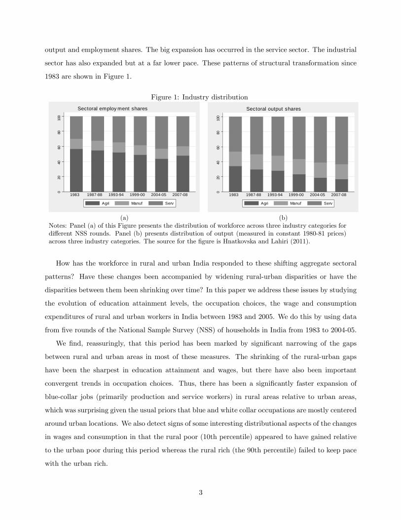
output and employment shares. The big expansion has occurred in the service sector. The industrial

sector has also expanded but at a far lower pace. These patterns of structural transformation since

1983 are shown in Figure 1.

Figure 1: Industry distribution

020

4060

8010

0

1983 1987­88 1993­94 1999­00 2004­05 2007­08

Sectoral employ ment shares

Agri Manuf Serv

020

4060

8010

0

1983 1987­88 1993­94 1999­00 2004­05 2007­08

Sectoral output shares

Agri Manuf Serv

(a) (b)Notes: Panel (a) of this Figure presents the distribution of workforce across three industry categories fordifferent NSS rounds. Panel (b) presents distribution of output (measured in constant 1980-81 prices)across three industry categories. The source for the figure is Hnatkovska and Lahiri (2011).

How has the workforce in rural and urban India responded to these shifting aggregate sectoral

patterns? Have these changes been accompanied by widening rural-urban disparities or have the

disparities between them been shrinking over time? In this paper we address these issues by studying

the evolution of education attainment levels, the occupation choices, the wage and consumption

expenditures of rural and urban workers in India between 1983 and 2005. We do this by using data

from five rounds of the National Sample Survey (NSS) of households in India from 1983 to 2004-05.

We find, reassuringly, that this period has been marked by significant narrowing of the gaps

between rural and urban areas in most of these measures. The shrinking of the rural-urban gaps

have been the sharpest in education attainment and wages, but there have also been important

convergent trends in occupation choices. Thus, there has been a significantly faster expansion of

blue-collar jobs (primarily production and service workers) in rural areas relative to urban areas,

which was surprising given the usual priors that blue and white collar occupations are mostly centered

around urban locations. We also detect signs of some interesting distributional aspects of the changes

in wages and consumption in that the rural poor (10th percentile) appeared to have gained relative

to the urban poor during this period whereas the rural rich (the 90th percentile) failed to keep pace

with the urban rich.

3

Our broad conclusion from these results is that the incentives generated by the institutional

structure of the country are providing useful signals to the workforce in guiding their choices. As a

result, there is significant churning that occurs at the micro levels of the economy in response to the

aggregate churning. Moreover, some of the changes have been truly striking with the median wage

premium of urban workers declining from around 100 percent in 1983 to just around 25 percent by

2005. This is a welcome sign.

There is a large body of work on inequality and poverty in India. A sample of this work can

be found in Banerjee and Piketty (2001), Bhalla (2003), Deaton and Dreze (2002) and Sen and

Himanshu (2005). While some of these studies do examine inequality and poverty in the context of

the rural and urban sectors separately (see Deaton and Dreze (2002) in particular), most of this work

is centered on either measuring inequality (through Gini coeffi cients) or poverty, focused either on

consumption or income alone, and restricted to a few rounds of the NSS data at best. An overview

of this work can be found in Pal and Ghosh (2007). Our study is distinct from this body of work in

that we examine multiple indicators of economic achievement over a 22 year period. This gives us

both a broader view of developments as well as a time-series perspective on post-reform India.

The rest of the paper is organized as follows: the next section presents the data and some sample

statistics. Section 3 presents the main results on changes in the rural-urban gaps while the last

section contains concluding thoughts.

2 Data

Our data comes from successive rounds of the National Sample Survey (NSS) of households in India

for employment and consumption. The survey rounds that we include in the study are 1983 (round

38), 1987-88 (round 43), 1993-94 (round 50), 1999-2000 (round 55), and 2004-05 (round 61). Since

our focus is on determining the trends in occupations and wages, amongst other things, we choose to

restrict the sample to individuals in the working age group 16-65, who are working full time (defined

as those who worked at least 2.5 days in the week prior to be being sampled), who are not enrolled

in any educational institution, and for whom we have both education and occupation information.

We further restrict the sample to individuals who belong to male-led households.2 These restrictions

leave us with, on average, 160,000 to 180,000 individuals per survey round.

The sample statistics across the rounds are given in Table 1. The table breaks down the overall

patterns by individuals and households and by rural and urban locations. Clearly, the sample is

2This avoids households with special conditions since male-led households are the norm in India.

4

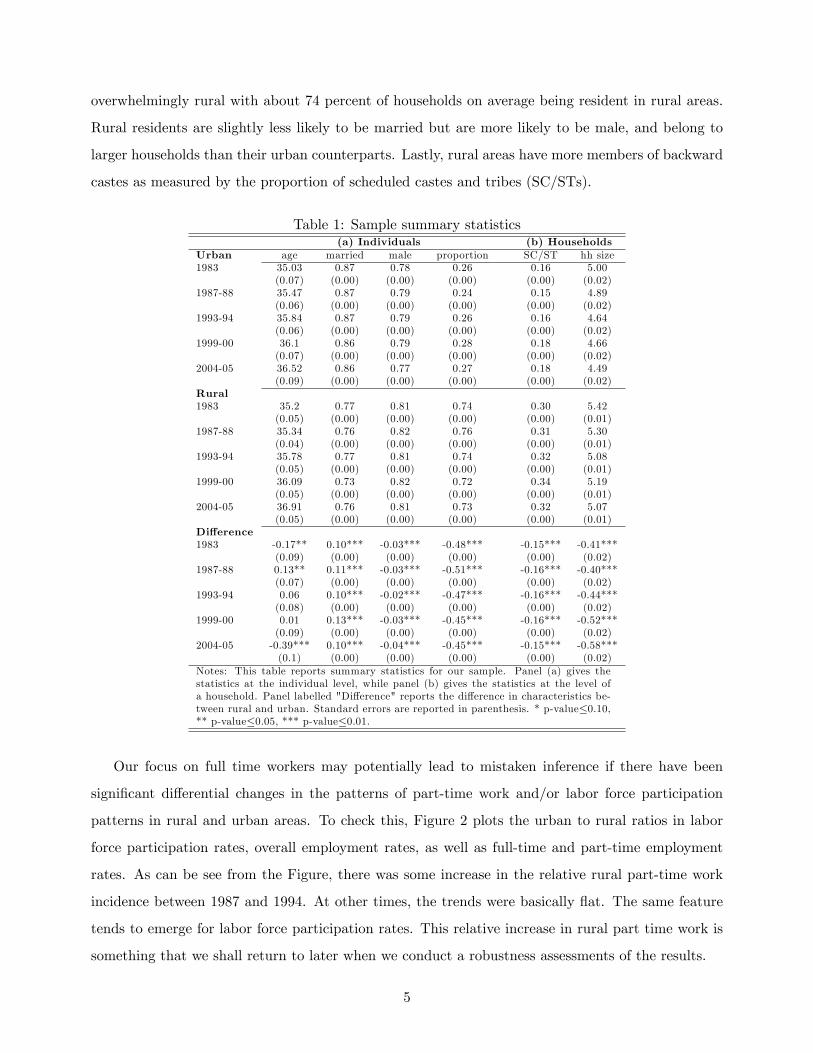
overwhelmingly rural with about 74 percent of households on average being resident in rural areas.

Rural residents are slightly less likely to be married but are more likely to be male, and belong to

larger households than their urban counterparts. Lastly, rural areas have more members of backward

castes as measured by the proportion of scheduled castes and tribes (SC/STs).

Table 1: Sample summary statistics(a) Individuals (b) Households

Urban age married male proportion SC/ST hh size1983 35.03 0.87 0.78 0.26 0.16 5.00

(0.07) (0.00) (0.00) (0.00) (0.00) (0.02)1987-88 35.47 0.87 0.79 0.24 0.15 4.89

(0.06) (0.00) (0.00) (0.00) (0.00) (0.02)1993-94 35.84 0.87 0.79 0.26 0.16 4.64

(0.06) (0.00) (0.00) (0.00) (0.00) (0.02)1999-00 36.1 0.86 0.79 0.28 0.18 4.66

(0.07) (0.00) (0.00) (0.00) (0.00) (0.02)2004-05 36.52 0.86 0.77 0.27 0.18 4.49

(0.09) (0.00) (0.00) (0.00) (0.00) (0.02)Rural1983 35.2 0.77 0.81 0.74 0.30 5.42

(0.05) (0.00) (0.00) (0.00) (0.00) (0.01)1987-88 35.34 0.76 0.82 0.76 0.31 5.30

(0.04) (0.00) (0.00) (0.00) (0.00) (0.01)1993-94 35.78 0.77 0.81 0.74 0.32 5.08

(0.05) (0.00) (0.00) (0.00) (0.00) (0.01)1999-00 36.09 0.73 0.82 0.72 0.34 5.19

(0.05) (0.00) (0.00) (0.00) (0.00) (0.01)2004-05 36.91 0.76 0.81 0.73 0.32 5.07

(0.05) (0.00) (0.00) (0.00) (0.00) (0.01)Difference1983 -0.17** 0.10*** -0.03*** -0.48*** -0.15*** -0.41***

(0.09) (0.00) (0.00) (0.00) (0.00) (0.02)1987-88 0.13** 0.11*** -0.03*** -0.51*** -0.16*** -0.40***

(0.07) (0.00) (0.00) (0.00) (0.00) (0.02)1993-94 0.06 0.10*** -0.02*** -0.47*** -0.16*** -0.44***

(0.08) (0.00) (0.00) (0.00) (0.00) (0.02)1999-00 0.01 0.13*** -0.03*** -0.45*** -0.16*** -0.52***

(0.09) (0.00) (0.00) (0.00) (0.00) (0.02)2004-05 -0.39*** 0.10*** -0.04*** -0.45*** -0.15*** -0.58***

(0.1) (0.00) (0.00) (0.00) (0.00) (0.02)Notes: This table reports summary statistics for our sample. Panel (a) gives thestatistics at the individual level, while panel (b) gives the statistics at the level ofa household. Panel labelled "Difference" reports the difference in characteristics be-tween rural and urban. Standard errors are reported in parenthesis. * p-value≤0.10,** p-value≤0.05, *** p-value≤0.01.

Our focus on full time workers may potentially lead to mistaken inference if there have been

significant differential changes in the patterns of part-time work and/or labor force participation

patterns in rural and urban areas. To check this, Figure 2 plots the urban to rural ratios in labor

force participation rates, overall employment rates, as well as full-time and part-time employment

rates. As can be see from the Figure, there was some increase in the relative rural part-time work

incidence between 1987 and 1994. At other times, the trends were basically flat. The same feature

tends to emerge for labor force participation rates. This relative increase in rural part time work is

something that we shall return to later when we conduct a robustness assessments of the results.

5

Figure 2: Labor force participation and employment gaps

.4.5

.6.7

.8.9

11.

1

1983 1987­88 1993­94 1999­00 2004­05

lfp employed full­time part­time

Relative labor market gaps

Note: "lfp" refers to the ratio of labor force participation rate of urban to rural sectors. "employed" refersto the ratio of employment rates for the two groups; while "full-time" and "part-time" are, respectively,the ratios of full-time employment rates and part-time employment rates of the two groups.

3 Rural-Urban Gaps

We now turn to our central goal of uncovering the gaps in the characteristics of the workforce between

rural and urban areas. More specifically, we are interested in determining the trends in these gaps

over the past 25 years. There are four indicators of primary interest: education attainments levels

of the workforce, the occupation distribution of the workforce, the wage levels of workers and their

consumption levels. In the following we shall present the levels of each of these indicators for the

two groups individually as well as the gaps between them.

3.1 Education

Our first indicator of interest is the education attainment level of the rural and urban workforce.

Education in the NSS data is presented as a category variable with the survey listing the highest

education attainment level in terms of categories such as primary, middle etc. In order to ease the

presentation we proceed in two ways. First, we construct a variable for the years of education. We

do so by assigning years of education to each category based on a simple mapping: not-literate =

0 years; literate but below primary = 2 years; primary = 5 years; middle = 8 years; secondary and

higher secondary = 10 years; graduate = 15 years; post-graduate = 17 years. Diplomas are treated

similarly depending on the specifics of the attainment level.3 Second, we use the reported education3We are forced to combine secondary and higher secondary into a combined group of 10 years because the higher

secondary classification is missing in the 38th and 43rd rounds. The only way to retain comparability across rounds

6

categories but aggregate them into five broad groups: 1 for illiterates, 2 for some but below primary

school, 3 for primary school, 4 for middle, and 5 for secondary and above. The results from the two

approaches are similar. While we use the second method for our econometric specifications since

these are the actually reported data as opposed to the years series that was constructed by us, we

also show results from the first approach below.

Table 2 shows the average years of education of the urban and rural workforce across the five

rounds in our sample. The two features that emerge from the table are that (a) education attainment

rates as measured by years of education were rising in both urban and rural sectors during this period;

and (b) the rural-urban education gap shrank monotonically over this period. The average years of

education of the urban worker was 164 percent higher than the typical rural worker in 1983 (5.83

years to 2.21 years). This advantage declined to 94 percent by 2004-05 (7.65 years to 3.94 years). To

put these numbers in perspective, in 1983 the average urban worker had slightly more than primary

education while the typical rural worker was literate but below primary. By 2004-05, the average

urban worker had about a middle school education while the typical rural worker had almost reached

primary education. While the overall numbers indicate the still dire state of literacy of the workforce

in the country, the movements underneath do indicate improvements over time with the rural workers

improving faster.

Table 2: Education Gap: Years of SchoolingAverage years of education Relative education gap

Overall Urban Rural Urban/Rural1983 3.01 5.83 2.21 2.64

(0.01) (0.03) (0.01) (0.02)1987-88 3.18 6.12 2.41 2.54

(0.01) (0.03) (0.01) (0.02)1993-94 3.86 6.85 2.98 2.30

(0.01) (0.03) (0.02) (0.02)1999-2000 4.37 7.39 3.43 2.15

(0.02) (0.04) (0.02) (0.02)2004-05 4.85 7.65 3.94 1.94

(0.02) (0.04) (0.02) (0.01)

Notes: This table presents the average years of education for the overall sample and separately for the urbanand rural workforce; as well as the relative gap in the years of education obtained as the ratio of urban torural education years. The reported statistics are obtained for each NSS survey round which is shown in thefirst column. Standard errors are in parenthesis.

Table 2, while revealing an uplifting trend for the average worker, nevertheless masks potentially

important underlying heterogeneity in education attainment by cohort, i.e., variation by the age of

the respondent. Figure 3 shows the relative gap in years of education between the typical urban and

rural worker by birth cohort. The point to note is that the gaps have been getting smaller by age:

then is to combine the two categories.

7

the younger the cohort the smaller the gap. Most strikingly, the average gap in 2004-05 between

urban and rural workers from the youngest birth cohort (born between 1982 and 1988) has almost

disappeared (about 25 percent) while the corresponding gap for that year for the 45-51 year old

workers born between 1954 and 1960 stood at 150 percent. Clearly, the declining rural-urban gaps

are being driven by declining education gaps amongst the younger workers in the two sectors.

Figure 3: Education gaps by birth cohorts

1.5

22.

53

3.5

1983 1987­88 1993­94 1999­00 2004­05

1919­25 1926­32 1933­39 1940­46 1947­531954­60 1961­67 1968­74 1975­81 1982­88

overall

Notes: The figure shows the relative gap in the average years of educationbetween the urban and rural workforce over time for different birth cohorts.

The time trends in years of education potentially mask the changes in the quality of education.

In particular, they fail to reveal what kind of education is causing the rise in years: is it people

moving from middle school to secondary or is it movement from illiteracy to some education? While

both movements would add a similar number of years to the total, the impact on the quality of

the workforce may be quite different. Further, we are also interested in determining whether the

movements in urban and rural areas are being driven by very different movement in the category of

education.

Panel (a) of Figure 4 shows the distribution of the urban and rural workforce by education

category. Recall that education categories 1, 2 and 3 are "illiterate", "some but below primary

education" and "primary", respectively. Hence in 1983, 55 percent of the urban labor force and over

80 percent of the rural labor force had primary or below education, reflecting the abysmal delivery

of public services in education in the first 35 years of post-independence India. By 2005, the primary

and below category had come down to 40 percent for urban workers and 60 percent for rural workers.

Simultaneously, the other notable trend during this period is the perceptible increase in the secondary

8

Figure 4: Education distribution0

2040

6080

100

URBAN RURAL

19831987­88

1993­941999­00

2004­051983

1987­881993­94

1999­002004­05

Distribution of workforce across edu

Edu1 Edu2 Edu3 Edu4 Edu5

01

23

45

1983 1987­88 1993­94 1999­00 2004­05

Gap in workforce distribution across edu

Edu1 Edu2 Edu3 Edu4 Edu5

(a) (b)Notes: Panel (a) of this figure presents the distribution of the workforce across five education categoriesfor different NSS rounds. The left set of bars refers to urban workers, while the right set is for ruralworkers. Panel (b) presents relative gaps in the distribution of urban relative to rural workers across fiveeducation categories. See the text for the description of how education categories are defined (category1 is the lowest education level - illiterate).

and above category for workers in both sectors. For the urban sector, this category expanded from

about 30 percent in 1983 to over 40 percent in 2005. Correspondingly, the share of the secondary

and higher educated rural worker rose from just around 5 percent of the rural workforce in 1983 to

about 22 percent in 2005. This, along with the decline in the proportion of rural illiterate workers

from 60 percent to around 30 percent, represent the sharpest and most promising changes in the

past 25 years.

Panel (b) of Figure 4 shows the changes in the relative education distributions of the urban

and rural workforce. For each survey year, the Figure shows the fraction of urban workers in each

education category relative to the fraction of rural workers in that category. Thus, in 1983 almost

30 percent of urban workers belonged to category 5 while only about 6 percent of rural workers

were in that education category. Hence, the height of the bar for category 5 is close to 5 for 1983

indicating that the urban worker is over-represented in the secondary and above category. Similarly,

about 24 percent of urban workers were illiterate in 1983 while almost 60 percent of rural workers

were illiterate. Thus, the bar for category 1 in 1983 was under 0.5, i.e., rural workers were over-

represented in that category. Clearly, the closer the height of the bars are to one the more symmetric

is the distribution of the two groups in that category while the further away from one they are, the

more skewed the distribution is. As the Figure indicates, the biggest convergence in the education

distribution between 1983 and 2005 appears to have been in categories 4 and 5 (middle and secondary

and above) where the bars shrank rapidly and a slightly more muted one in category 1 (illiterates)

9

where the bar increased in height over time.

While the visual impressions suggest convergence in education, are these trends statistically

significant? We turn to this issue next by estimating ordered multinomial probit regressions of

education categories 1 to 5 on a constant and the rural dummy. The aim is to ascertain the significance

of the difference between rural and urban areas in the probability of a worker belonging to each

category as well as the significance of changes over time in these differences. Table 3 shows the

results.

Table 3: Marginal Effect of rural dummy in ordered probit regression for education categoriesPanel (a): Marginal effects, unconditional Panel (b): Changes

1983 1987-88 1993-94 1999-2000 2004-05 83 to 93 93 to 05 83 to 05Edu 1 0.3522*** 0.3437*** 0.3176*** 0.3028*** 0.2638*** -0.0346*** -0.0538*** -0.0884***

(0.0029) (0.0025) (0.0025) (0.0027) (0.0027) (0.0038) (0.0037) (0.004)Edu 2 0.0032*** 0.0090*** 0.0214*** 0.0274*** 0.0374*** 0.0182*** 0.016*** 0.0342***

(0.0005) (0.0005) (0.0005) (0.0006) (0.0008) (0.0007) (0.0009) (0.0009)Edu 3 -0.0474*** -0.0389*** -0.0163*** -0.0008* 0.0120*** 0.0311*** 0.0283*** 0.0594***

(0.0007) (0.0005) (0.0004) (0.0005) (0.0006) (0.0008) (0.0008) (0.0009)Edu 4 -0.0916*** -0.0782*** -0.0655*** -0.0535*** -0.0452*** 0.0261*** 0.0203*** 0.0464***

(0.0011) (0.0009) (0.0008) (0.0007) (0.0007) (0.0014) (0.0011) (0.0013)Edu 5 -0.2165*** -0.2357*** -0.2573*** -0.2758*** -0.2681*** -0.0408*** -0.0107*** -0.0516***

(0.0025) (0.0023) (0.0026) (0.0031) (0.0035) (0.0036) (0.0044) (0.0043)

N 164739 183914 162534 172682 168541Notes: Panel (a) reports the marginal effects of the rural dummy in an ordered probit regression of education categories 1to 5 on a constant and a rural dummy for each survey round. Panel (b) of the table reports the change in the marginaleffects over successive decades and over the entire sample period. N refers to the number of observations. Standard errorsare in parenthesis. * p-value≤0.10, ** p-value≤0.05, *** p-value≤0.01.

Panel (a) of the Table shows that the marginal effect of the rural dummy was significant for

all rounds and all categories. The rural dummy significantly raised the probability of belonging to

education categories 1 and 2 ("illiterate" and "some but below primary education", respectively)

while it significantly reduced the probability of belonging to categories 3-5. Panel (b) of Table 3

shows that the changes over time in these marginal effects were also significant for all rounds and

all categories. The trends though are interesting. There are clearly significant convergent trends

for education categories 1, 3 and 4. Category 1, where rural workers were over-represented in 1983

saw a declining marginal effect of the rural dummy. Categories 3 and 4 (primary and middle school,

respectively), where rural workers were under-represented in 1983 saw a significant increase in the

marginal effect of the rural status. Hence, the rural under-representation in these categories declined

significantly. Categories 2 and 5 however were marked by a divergence in the distribution. Category

2, where rural workers were over-represented saw an increase in the marginal effect of the rural

dummy while in category 5, where they were under-represented, the marginal effect of the rural

dummy became even more negative. This divergence though is not inconsistent with Figure 4. The

figure shows trends in the relative gaps while the probit regressions show trends in the absolute gaps.

10

In summary, the overwhelming feature of the data on education attainment gaps suggests a strong

and significant trend toward education convergence between the urban and rural workforce. This is

evident when comparing average years of education, the relative gaps by education category as well

as the absolute gaps between the groups in most categories.

3.2 Occupation Choices

We now turn to our second measure of interest: the occupation choices being made by the workforce

in urban and rural areas. Our interest lies in determining whether the occupation choices being

made in the two sectors are showing some signs of convergence? Clearly, there are some fundamental

differences in the sectoral compositions of rural and urban areas making it unlikely/impossible for

the occupation distributions to converge. However, the country as a whole has been undergoing a

structural transformation with an increasing share of output accruing to services and a corresponding

decline in the output share of agriculture. Are these trends translating into symmetric changes in

rural and urban occupation distributions? Or, is the expansion of the non-agricultural sector (broadly

defined) restricted to urban areas?

To examine this issue, we aggregate the reported 3-digit occupation categories in the survey into

three broad occupation categories: Occ 1 which comprises white collar occupations like administra-

tors, executives, managers, professionals, technical and clerical workers; Occ 2 comprises blue collar

occupations such as sales workers, service workers and production workers; Occ 3 collects farmers,

fishermen, loggers, hunters etc.. Figure 5 shows the distribution of these occupations in urban and

rural India across the survey rounds (Panel (a)) as well as the gap in these distributions between the

sectors (Panel (b)).

The urban and rural occupation distributions have the obvious feature that urban areas have

a much smaller fraction of the workforce in agrarian occupations (Occ 3) while rural areas have

a miniscule share of people working in white collar jobs (Occ 1). The crucial aspect though is the

share of the workforce in Occ 2 which collects essentially blue collar jobs that pertain to both services

and manufacturing. The urban sector clearly has a dominance of these occupations. Importantly

though, the share of Occ 2 has been rising not just in urban areas but also in rural areas. In fact,

as Panel (b) of Figure 5 shows, the share of both white collar and blue collar jobs in rural areas are

rising faster than their corresponding shares in urban areas. This suggests that the overall structural

transformation at the level of output is translating into convergent trends in the occupation structure

across rural and urban sectors.

11

Figure 5: Occupation distribution0

2040

6080

100

URBAN RURAL

19831987­88

1993­941999­00

2004­051983

1987­881993­94

1999­002004­05

Distribution of workforce across occ

Occ1 Occ2 Occ3

02

46

1983 1987­88 1993­94 1999­00 2004­05

Gap in workforce distribution across occ

Occ1 Occ2 Occ3

(a) (b)Notes: Panel (a) of this figure presents the distribution of workforce across three occupation categoriesfor different NSS rounds. The left set of bars refers to urban workers, while the right set is for ruralworkers. Panel (b) presents relative gaps in the distribution of urban relative to rural workers across thethree occupation categories. Occ 1 collects white collar workers, Occ 2 collects blue collar workers, whileOcc 3 refers to farmers and other agricultural workers.

Is this visual image of sharp changes in the occupation distribution and convergent trends sta-

tistically significant? To examine this we estimate a multinomial probit regression of occupation

choices on a rural dummy and a constant for each survey round. The results for the marginal effects

of the rural dummy are shown in Table 4. The rural dummy has significantly negative marginal

effect on the probability of being in both Occ 1 (white collar jobs) and Occ 2 (blue collar jobs),

while having significantly positive effects on the probability of being in agrarian/pastoral jobs (Occ

3). However, as Panel (b) of the Table indicates, between 1983 and 2005 the negative effect in Occ

2 has declined (the marginal effect has become less negative) while the positive effect on being in

Occ 3 has become smaller, with both changes being significant at the 1 percent level. Since there

was an initial under-representation of Occ 2 and over-representation of Occ 3 in rural jobs, we view

these results as indicating an ongoing process of statistical convergence across rural and urban areas

in these two occupation.

3.3 Wages

The next point of interest is the behavior of wages in urban and rural India. Wages are obtained as

the daily wage/salaried income received for the work done by respondents during the previous week

(relative to the survey week). Wages can be paid in cash or kind, where the latter are evaluated at

the current retail prices. We convert wages into real terms using state-level poverty lines that differ

for rural and urban sectors. We express all wages in 1983 rural Maharashtra poverty lines.

12

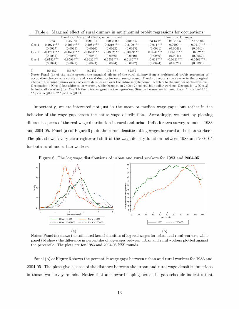
Table 4: Marginal effect of rural dummy in multinomial probit regressions for occupationsPanel (a): Marginal effects, unconditional Panel (b): Changes

1983 1987-88 1993-94 1999-2000 2004-05 83 to 93 93 to 05 83 to 05Occ 1 -0.1971*** -0.2067*** -0.2081*** -0.2219*** -0.2190*** -0.011*** -0.0109** -0.0219***

(0.0027) (0.0025) (0.0026) (0.0032) (0.0035) (0.0041) (0.0048) (0.0044)Occ 2 -0.4781*** -0.4529*** -0.4540*** -0.4332*** -0.3999*** 0.0241*** 0.0541*** 0.0782***

(0.0032) (0.0030) (0.0031) (0.0036) (0.0040) (0.0039) (0.0041) (0.0052)Occ 3 0.6752*** 0.6596*** 0.6622*** 0.6551*** 0.6189*** -0.013*** -0.0433*** -0.0563***

(0.0024) (0.0021) (0.0023) (0.0024) (0.0027) (0.0024) (0.0023) (0.0036)

N 164482 181765 162457 171153 167857Note: Panel (a) of the table present the marginal effects of the rural dummy from a multinomial probit regression ofoccupation choices on a constant and a rural dummy for each survey round. Panel (b) reports the change in the marginaleffects of the rural dummy over successive decades and over the entire sample period. N refers to the number of observations.Occupation 1 (Occ 1) has white collar workers, while Occupation 2 (Occ 2) collects blue collar workers. Occupation 3 (Occ 3)includes all agrarian jobs. Occ 3 is the reference group in the regression. Standard errors are in parenthesis. * p-value≤0.10,** p-value≤0.05, *** p-value≤0.01.

Importantly, we are interested not just in the mean or median wage gaps, but rather in the

behavior of the wage gap across the entire wage distribution. Accordingly, we start by plotting

different aspects of the real wage distribution in rural and urban India for two survey rounds —1983

and 2004-05. Panel (a) of Figure 6 plots the kernel densities of log wages for rural and urban workers.

The plot shows a very clear rightward shift of the wage density function between 1983 and 2004-05

for both rural and urban workers.

Figure 6: The log wage distributions of urban and rural workers for 1983 and 2004-05

0.2

.4.6

.8de

nsity

0 1 2 3 4 5log wage  (real)

Urban ­ 1983 Rural  ­ 1983Urban ­ 2004­05 Rural  ­ 2004­05

­.3­.2

­.10

.1.2

.3.4

.5.6

.7.8

lnw

age(

Urb

an)­

lnw

age(

Rur

al)

0 10 20 30 40 50 60 70 80 90 100percent ile

1983 2004­05

(a) (b)Notes: Panel (a) shows the estimated kernel densities of log real wages for urban and rural workers, whilepanel (b) shows the difference in percentiles of log-wages between urban and rural workers plotted againstthe percentile. The plots are for 1983 and 2004-05 NSS rounds.

Panel (b) of Figure 6 shows the percentile wage gaps between urban and rural workers for 1983 and

2004-05. The plots give a sense of the distance between the urban and rural wage densities functions

in those two survey rounds. Notice that an upward sloping percentile gap schedule indicates that

13

wage gaps are rising for richer wage groups. Also, if the schedule for one round lies to the right of the

schedule for another survey round for some range of percentiles then it indicates that the wage gap

has shrunk across those rounds for those percentiles. The plot for 2004-05 lies to the right of that

for 1983 till the 70th percentile indicating that for most of the wage distribution, the gap between

urban and rural wages has declined over this period. Indeed, it is easy to see from Panel (b) that the

median log wage gap between urban and rural wages fell from around 0.7 to around 0.2. Hence, the

median wage premium of urban workers declined from round 100 percent to 26 percent. Between

the 70th and 90th percentiles however, the wage gaps are larger in 2004-05 as compared to 1983. A

last noteworthy feature is that in 2004-05, for the bottom 15 percentiles of the wage distribution in

the two sectors, rural wages were actually higher than urban wages. This was in stark contrast to

the picture in 1983 when urban wages were higher than rural wages for all percentiles.

Figure 6 gives the sense of wage convergence between rural and urban areas. But is this borne

out statistically, and if so, are the patterns significant? To test for this, we estimate Recentered

Influence Function (RIF) regressions developed by Firpo, Fortin, and Lemieux (2009) of the log real

wages of individuals in our sample on a constant, controls for age (we include age and age squared

of each individual) and a rural dummy for each survey round. Our interest is in the coeffi cient on

rural dummy, its significance and changes over time. The controls for age are intended to flexibly

control for the fact that wages are likely to vary with age and experience. We perform the analysis

for different unconditional quantiles as well as the mean of the wage distribution.4

Table 5: Wage gaps and changesPanel (a): Rural dummy coeffi cient Panel (b): Changes

1983 1993-94 1999-2000 2004-05 1983 to 1993-94 1993 to 2004-05 1983 to 2004-0510th quantile -0.2073*** -0.0318*** -0.0126 0.0201* 0.1755*** 0.0519*** 0.2274***

(0.0105) (0.0089) (0.0085) (0.0121) (0.0138) (0.0151) (0.016)50th quantile -0.5874*** -0.4037*** -0.3694*** -0.2282*** 0.1837*** 0.1755*** 0.3592***

(0.0089) (0.0079) (0.0085) (0.0089) (0.0119) (0.0119) (0.0126)90th quantile -0.5020*** -0.5531*** -0.6916*** -0.7133*** -0.0511** -0.1602*** -0.2113***

-0.0141 -0.0167 -0.0238 -0.0285 (0.0218) (0.033) (0.0318)mean -0.5097*** -0.3951*** -0.4121*** -0.3051*** 0.1146*** 0.09*** 0.2046***

(0.0076) (0.0086) (0.0096) (0.0100) (0.0115) (0.0132) (0.0126)

N 63808 63057 66820 61111Note: Panel (a) of this table reports the estimates of coeffi cients on the rural dummy from RIF regressions of log wages on ruraldummy, age, age squared, and a constant. Results are reported for the 10th, 50th and 90th quantiles. Row labelled "mean"reports the rural coeffi cient from the conditional mean regression. Panel (b) reports the changes in the estimated coeffi cientsover successive decades and the entire sample period. N refers to the number of observations. Standard errors are in parenthesis.* p-value≤0.10, ** p-value≤0.05, *** p-value≤0.01.

4We use the RIF approach (developed by Firpo, Fortin, and Lemieux (2009)) because we are interested in estimatingthe effect of the rural dummy for different points of the distribution, not just the mean. However, since the law ofiterated expectations does not go through for quantiles, we cannot use standard regression methods to determine theunconditional effect of rural status on wages for different quantiles. The RIF methodology essentially gets around thisproblem for quantiles. Details regarding this meethod can be found in Firpo, Fortin, and Lemieux (2009) and in anonline appendix that accompanies this paper.

14

Panel (a) of Table 5 reports the estimated coeffi cient on the rural dummy for the 10th, 50th and

90th percentiles as well as the mean for different survey rounds.5 Clearly, rural status significantly

reduces wages across rounds and percentiles of the distribution. However, the size of the negative

rural effect has become significantly smaller over time for the 10th and 50th percentiles as well as the

mean over the entire period as well all sub-periods within (see Panel (b)) with the largest convergence

having occurred for the median. Interestingly, it is only the 90th percentile for which the wage gap

actually increased. These results corroborate the visual impression from Figure 6: the wage gap

between rural and urban areas fell between 1983 and 2005 for all but the richest wage groups.

While the wage convergence for most of the distribution is interesting, what were the factors

driving this convergence? We turn to this issue next. Our focus is on two aspects of the wage

gaps: Was the wage convergence documented above driven by a convergence of measured covariates

of wages; or was it due to changes in unmeasured factors? We proceed with an adaptation of the

Oaxaca-Blinder decomposition technique to quantiles by using the RIF methods. The key twist to

our approach relative to the standard decomposition of gaps is that we are decomposing changes in

the gaps across rounds rather than decomposing gaps at a point in time. This adds an extra layer

to the decomposition process.6

In the decompositions we are interested in assessing the contribution of explained factors to the

wage convergence and the unexplained factors. Our set of explained factors includes demographic

characteristics such as individual’s age, age squared, caste, religion, and state of residence. Ad-

ditionally, we control for the education level of the individual by including dummies for education

categories 1-5. Note that we control for caste by including a dummy for whether or not the individual

is an SC/ST in order to control for the fact that SC/STs tend to be disproportionately rural. Given

that they are also disproportionately poor and have little education, controlling for SC/ST status

seems important in order to determine the independent effect of rural status on wages.

Table 6 shows the results of the decomposition exercise. Panel (a) shows the decomposition of

the measured gap (column (i)) into the explained and unexplained components (columns (ii) and

(iii)), as well as the part of the gap that is explained by education alone (column (iv)). Clearly,

education is an important covariate of the rural urban wage gap. Differential changes in education

attainment levels explain 19 percent of the change in wage gap for the 10th percentile, 25 percent

5Due to an anomalous feature of missing rural wage data for 1987-88, we chose to drop 1987-88 from the study ofwages in order to avoid spurious results.

6All decompositions are performed using a pooled model across rural and urban sectors as the reference model.Following Fortin (2006) we allow for a group membership indicator in the pooled regressions. We also used 1983 roundas the benchmark sample. Details of the decomposition method can be found in an online Appendix accomplanyingthe paper.

15

Table 6: Decomposing changes in rural-urban wage gaps over time(a). Change (1983 to 2004-05) explained

(i) measured gap (ii) explained (iii) unexplained (iv) education10th quantile -0.2882*** -0.0489*** -0.2392*** -0.0520***

(0.0359) (0.0158) (0.0348) (0.0110)50th quantile -0.4346*** -0.1313*** -0.3033*** -0.1069***

(0.0231) (0.0163) (0.0190) (0.0134)90th quantile 0.1948*** 0.2427*** -0.0479 0.2255***

(0.0380) (0.0403) (0.0416) (0.0323)(b). Change in explained component10th quantile -0.0489*** -0.0351*** -0.0139 -0.0323***

(0.0158) (0.0085) (0.0145) (0.0050)50th quantile -0.1313*** -0.0329** -0.0984*** -0.0305***

(0.0163) (0.0133) (0.0122) (0.0090)90th quantile 0.2427*** 0.0321 0.2106*** 0.0396**

(0.0403) (0.0207) (0.0356) (0.0186)

Note: Panel (a) presents the change in the rural-urban wage gap between 1983 and 2004-05. Panel (b) reports thedecomposition of the time-series change in the explained component of the change in the wage gap over 1983-2004-05period. All gaps are decomposed into explained and unexplained components using the RIF regression approach of Firpo,Fortin, and Lemieux (2009) for the 10th, 50th and 90th quantiles. Both panels also report the contribution of education tothe explained gaps. Bootstrapped standard errors are in parenthesis. * p-value≤0.10, ** p-value≤0.05, *** p-value≤0.01.

for the 50th percentile and almost 40 percent of the widening gap for the 90th percentile of wages.

The other noteworthy aspect of the results is that most of the overall change in the wage gap is not

accounted for by the included covariates. This is an important feature of our results which we shall

return to below.

If the explained component of a regression is βX then changes in that component itself have

two components: the change in X and the change β which is the measured return to X. Since X

is measured in the data, the part of the change in the explained component that is due to X is

"explained" by the data while the part due to β is not directly explained. Panel (b) of the Table 6

decomposed changes in the explained component itself into the explained and unexplained parts. For

the 10th percentile, most of the change in the measured component of the gap was due to changes in

the explained part (or X). For the median and the 90th percentile however, most of the change in

the explained component was due to changes in returns rather than changes in the component itself.

Overall, our conclusion from the wage data is that wages have converged significantly between

rural and urban India during since 1983 for all except the very top of the income distribution.

Education has been an important contributor to these convergent patterns. However, a majority of

the trend is due to unmeasured factors.

3.4 Consumption

Our last indicator of interest is the household expenditure on consumption in rural and urban India.

This measure is the one that is often used in studies on poverty and inequality. The variable we

16

use is monthly per capita household consumption expenditure, or "mpce". This variable is collected

at the level of the household, which implies that there is one observation per household rather

than individual level observations that we have been examining before. We convert consumption

expenditures into real terms using offi cial state-poverty lines, with rural Maharashtra in 1983 as the

base —same as we did for wages. In order to make real consumption results comparable with the

wage data, we convert consumption into per-capita daily value terms.

We start by plotting the kernel densities of the log of real consumption (we will use mpce and

consumption interchangeably from hereon) for rural and urban households for 1983 and 2004-05 in

Panel (a) of Figure 7. Panel (b) of the Figure plots the percentile gaps in per capita log household

consumption between urban and rural households for these two survey rounds (computed as urban

(log) mpce - rural (log) mpce).

Figure 7: The log consumption distributions of urban and rural households for 1983 and 2004-05

0.2

.4.6

.81

dens

ity

­2 0 2 4 6log consumption (real)

Urban ­ 1983 Rural ­ 1983Urban ­ 2004­05 Rural ­ 2004­05

­.10

.1.2

.3.4

.5ln

mpc

e(U

rban

)­ln

mpc

e(R

ural

)

0 10 20 30 40 50 60 70 80 90 100percentile

1983 2004­05

(a) (b)Notes: Panel (a) shows the estimated kernel densities of log per capita real consumption expenditurefor urban and rural households, while panel (b) shows the difference in percentiles of log-consumptionbetween urban and rural households plotted against the percentile. The plots are for the 1983 and 2004-05NSS rounds.

Panel (a) of Figure 7 shows that the consumption distribution shifted to the right for both rural

and urban households during this period. Panel (b) of the figure, which plots the gaps for each

percentile however shows an interesting feature. The plot for 2004-05 is significantly steeper than

the schedule for 1983. Effectively, the consumption gaps between urban and rural areas declined up

to about the median of the consumption distribution but widened above the median. Interestingly,

rural households till around the 30th percentile actually consumed more than their counterparts in

urban areas in 2004-05 (the gaps were negative) whereas the gaps were positive in 1983. Thus, the

rural poor have clearly done better than the urban poor during this period, as measured by their

17

household consumption levels.7 This is an interesting finding in its own right and may indicate the

effects of weaker social and family insurance mechanisms in urban areas for the poor which leads

them to possibly consume more than they would otherwise. This channel has been suggested as a

rationalization for low inequality and mobility in rural India by Munshi and Rosenzweig (2009).

Are the measured consumption gaps shown in Panel (b) of Figure 7 significant? Are the changes

in the gaps over time significant? We address this by estimating RIF regressions (which we described

in the previous subsection) of log consumption on a constant and a rural dummy for all the survey

rounds. We estimate these regressions for the 10th, 50th and 90th percentiles. We also run a

standard OLS specification to determine the effect of rural status on the unconditional mean of log

consumption. The results are reported in Table 7.

Table 7: Consumption gaps and changesPanel (a): Rural dummy coeffi cient

1983 1987-88 1993-94 1999-2000 2004-0510th quantile -0.0422*** 0.0491*** 0.0089 0.0209*** 0.0783***

-0.0084 -0.0077 -0.007 -0.008 -0.009250th quantile -0.0677*** -0.0393*** -0.0886*** -0.0965*** -0.0743***

-0.0065 -0.0056 -0.0054 -0.0063 -0.00790th quantile -0.1660*** -0.1807*** -0.2902*** -0.3574*** -0.4165***

-0.0115 -0.0103 -0.0111 -0.0125 -0.0156mean -0.0863*** -0.0555*** -0.1149*** -0.1344*** -0.1219***

-0.006 -0.0055 -0.0051 -0.0059 -0.007

N 87195 93638 86738 88345 87377Panel (b): Changes

1983 to 1993-94 1993 to 2004-05 1983 to 2004-0510th quantile 0.0511*** 0.0694*** 0.1205***

(0.0109) (0.0116) (0.0125)50th quantile -0.0209** 0.0142 -0.0067

(0.0085) (0.0089) (0.0096)90th quantile -0.1242*** -0.1263*** -0.2505***

(0.016) (0.0192) (0.0194)mean -0.0286*** -0.007 -0.0356***

(0.0079) (0.0087) (0.0092)

Note: Panel (a) reports the estimates of the coeffi cient on the rural dummy from RIF regressions of log consumptionexpenditures on rural dummy and a constant. Panel (b) reports the changes in the estimated coeffi cients over successivedecades and the entire sample period. N refers to the number of observations. Standard errors are in parenthesis. *p-value≤0.10, ** p-value≤0.05, *** p-value≤0.01.

For all except the 10th percentile of households, rural consumption expenditure was significantly

lower than the corresponding urban consumption across the survey rounds. The rural dummy for the

10th percentile regression was significantly negative in 1983 but turned positive and significant for

all subsequent rounds indicating that rural consumption became higher than urban consumption for

this group. Panel (b) of Table 7 shows that between 1983 and 2005 there was significant convergence

7Note that these findings are similar in nature to the results we obtained for wages though the specifics are different.In particular, for wages the gap shrank for a much larger portion of the distribution than the corresponding narrowingof expenditure gaps in 2004-05.

18

for the 10th percentile and the median, virtually no change in the consumption gap for the median,

and a significant divergence in consumption levels of the 90th percentile, i.e., the gap between the

richest groups in urban and rural India widened during this period.

A further point of interest is the source of the changes documented in Table 7, i.e., were the

consumption gaps changing over time due to changes in measured covariates of consumption or were

they due to unexplained factors? In order to determine this we conduct a Oaxaca-Blinder type time

series decomposition of the measured changes into their explained and unexplained components. We

do this using the RIF regression outlined above for different quantiles of the consumption distributions

in rural and urban areas. As covariates of consumption we introduce controls for household size,

the number of earning members of the household, state dummies, a caste dummy for SC/ST status,

and a religion dummy for Muslim status. We also control for the education characteristics of the

household by adding the education attainment level of the household head and the highest level of

education attained in the household. Table 7 shows the results of the decomposition.

Table 8: Decomposing changes in rural-urban consumption expenditure gaps over time(a). Change (1983 to 2004-05) explained

(i) measured gap (ii) explained (iii) unexplained (iv) education10th quantile -0.1289*** -0.0198** -0.1091*** -0.0035

(0.0173) (0.0090) (0.0186) (0.0056)50th quantile 0.0201 -0.0102 0.0303** 0.0021

(0.0164) (0.0094) (0.0139) (0.0044)90th quantile 0.2140*** 0.0626*** 0.1514*** 0.0167**

(0.0241) (0.0186) (0.0235) (0.0084)(b). Change in explained component10th quantile -0.0198** -0.0043 -0.0155** 0.0075**

(0.0090) (0.0054) (0.0074) (0.0034)50th quantile -0.0102 0.0086 -0.0188*** 0.0093**

(0.0094) (0.0063) (0.0066) (0.0037)90th quantile 0.0626*** 0.0393*** 0.0232 0.0142***

(0.0186) (0.0095) (0.0158) (0.0042)

Note: Panel (a) presents the change in the urban-rural consumption gap between 1983 and 2004-05. Panel (b) reports thedecomposition of the time-series change in the explained component of the change in the consumption gap over 1983—2004-05 period. All gaps are decomposed into explained and unexplained components using RIF regression approach of Firpo,Fortin, and Lemieux (2009). Both panels also report the contribution of education to the explained gaps. Bootstrappedstandard errors are in parenthesis. * p-value≤0.10, ** p-value≤0.05, *** p-value≤0.01.

The two aspects of this decomposition that we find noteworthy are: (a) the explained part of

the changes in the consumption gaps accounted for by the household and other covariates comprises

between 15 percent of the total change for the 10th percentile and 30 percent for the 90th percentile

(the change for the median was not statistically significantly different from zero). Hence, the majority

of the changes in the quantile gaps were driven by unexplained or unmeasured factors. This aspect

is similar to the results we obtained for wages. Second, changes in the education level of households

did not explain much of the actual change in the rural-urban consumption gap. This is in contrast to

19

changes in the rural-urban wage gaps where we found that education played a larger and significant

role.

4 Conclusion

We have examined and contrasted the patterns of economic change in rural and urban India over

the past three decades. We have found this period has been marked by a sharp and significant

convergent trend in the education attainment levels of the rural workforce towards the levels of their

urban counterparts. This process has also been accompanied by some convergence in the occupation

choices being made in the two sectors. Specifically, the contraction in agrarian jobs in rural areas

that has accompanied the ongoing structural transformation of economy away from agriculture has

been met by an expansion of blue-collar occupations in rural areas at a significantly faster rate than

the corresponding expansion of blue-collar occupations in urban areas. As a result there appears to

have set in a process of convergence in the rural and urban occupation distribution as well (even

though the absolute differences between the two sectors continues to be very large). Moreover, there

has also been a significant convergent trend in rural wages towards urban areas over this period with

the median urban wage premium having declined from 100 percent in 1983 to around 26 percent by

2005. We find this rate of wage convergence to be very large and somewhat unexpected.

We also found that the convergence in consumption between rural and urban households has been

more muted than that for some of the other indicators we examined. Importantly though there were

some shared features of the consumption and wage dynamics in that the rural poor did better over

time than the corresponding urban poor (10th percentile) in terms of both indicators so that by 2005,

the 10th percentile wage and consumption in rural areas exceeded that of their urban counterparts.

There was however divergence in the fortunes of the 90th percentile in both wages and consumption

where the pre-existing urban advantage became more pronounced over time.

We believe these results to be indicative of the fact that the massive macroeconomic changes that

have been underway in India during this period have led to a healthy churning of the labor force

in the country. The results we have obtained here for the rural-urban gaps are similar in spirit to

those in Hnatkovska, Lahiri, and Paul (2012) and Hnatkovska, Lahiri, and Paul (2011) for the gaps

between scheduled castes/tribes and others in the Indian workforce. There too we found significant

convergence across the two groups in education, occupation choices, wages and consumption. Clearly,

some of the market incentives that were unleashed by the economic reforms have been providing the

right signals to economic agents to make the appropriate market based private choices in terms of

20

their schooling and employment decisions.

21

References

Alesina, A., and D. Rodrik (1994): “Distributive Politics and Economic Growth,”The Quarterly

Journal of Economics, 109(2), 465—90.

Banerjee, A., and T. Piketty (2001): “Are the rich growing richer: Evidence from Indian tax

data,”Working papers, MIT and CEPREMAP.

Bhalla, S. S. (2003): “Recounting the poor: Poverty in India, 1983-99,”Economic and Political

Weekly, pp. 338—349.

Deaton, A., and J. Dreze (2002): “Poverty and inequality in India: A re-examination,”Economic

and Political Weekly, pp. 3729—3748.

Firpo, S., N. M. Fortin, and T. Lemieux (2009): “Unconditional Quantile Regressions,”Econo-

metrica, 77(3), 953—973.

Fortin, N. M. (2006): “Greed, Altruism, and the Gender Wage Gap,”Working papers, University

of British Columbia.

Harris, J. R., and M. P. Todaro (1970): “Migration, Unemployment and Development: A

Two-Sector Analysis,”American Economic Review, 60(1), 126—142.

Hnatkovska, V., and A. Lahiri (2011): “Convergence Across Castes,”Igc working papers, Inter-

national Growth Center.

Hnatkovska, V., A. Lahiri, and S. Paul (2011): “Breaking the Caste Barrier: Intergenerational

Mobility in India,”Working papers, University of British Columbia.

Hnatkovska, V., A. Lahiri, and S. Paul (2012): “Castes and Labor Mobility,”American Eco-

nomic Journal: Applied Economics forthcoming.

Kuznets, S. (1955): “Economic growth and income inequality,”American Economic Review, 45(1),

1—28.

Lewis, A. (1954): “Economic development with unlimited supply of labour,” The Manchester

School, 22(2), 139—191.

Munshi, K., and M. Rosenzweig (2009): “Why is Mobility in India so Low? Social Insurance,

Inequality, and Growth,”Working papers, Brown University, Department of Economics.

22

Pal, P., and J. Ghosh (2007): “Inequality in India: A survey of recent trends,”DESA Working

Papers 45, UN.

Persson, T., and G. Tabellini (1994): “Is Inequality Harmful for Growth?,”American Economic

Review, 84(3), 600—621.

Sen, A., and Himanshu (2005): “Poverty and inequality in India: Getting closer to the truth,”in

Data and Dogma: The Great Indian Poverty Debate, ed. by A. Deaton, and V. Kozel. Macmillan,

New Delhi.

23