The Round Trip Effect:Endogenous Transport Costs and International

Trade

Woan Foong Wong∗†

February 2018

Abstract

Ocean containerships transport the bulk of international trade flows and travelin fixed round trip routes. This paper studies this round trip effect, which linkstwo-way transport supply between locations. I show that this effect mitigatesshocks on one-direction trade and generates opposite-direction spillovers with thesame partner. Import tariff increases can therefore translate into potential exporttaxes. I develop an IV using this effect to estimate a containerized trade elastic-ity. Using these results, I estimate and simulate a counterfactual import tariffsincrease. My model predicts a 0.2% export price tax when doubling US importtariffs from a 1.2% average.

∗I am extremely grateful to Robert W. Staiger, L.Kamran Bilir, and Alan Sorensen for their invaluable guidance and support.I especially thank Robert W. Staiger for financial support. I also thank Enghin Atalay, Andrew B. Bernard, Emily J. Blanchard,Bruce Blonigen, Diego Comin, Steven N. Durlauf, Charles Engel, James D. Feyrer, Teresa Fort, Jesse Gregory, Douglas A. Irwin,Robert C. Johnson, Rasmus Lentz, Erzo F.P. Luttmer, John Kennan, Erin T. Mansur, Nancy Peregrim Marion, Paul Novosad,Nina Pavcnik, Christopher M. Snyder, Christopher Taber, Thomas Youle, and Oren Ziv for extremely insightful suggestions anddiscussions. Finally, I am thankful to Mark Colas, Andrea Guglielmo, Chenyan Lu, Yoko Sakamoto, Kegon Tan, Nathan Yoder,as well as many workshop, conference, and seminar participants for helpful comments. All remaining errors are my own.†Department of Economics, University of Oregon, Eugene, OR 97403. Email: wfwong@uoregon.edu

1 Introduction

“If transport costs varied with volume of trade, the [iceberg transport costs]would not be constants. Realistically, since there are joint costs of a round trip,[the going and return iceberg costs] will tend to move in opposite directions,depending upon the strengths of demands for east and west transport.”

Samuelson (1954), p. 270, fn. 2

The cost of transporting goods from origin to destination is determined in equi-librium by the interaction between the supply and demand for transportation betweenthese locations. Additionally, carriers, such as containerships and airplanes, travel infixed routes and have to return to the origin in order to fulfill demand (Pigou and Taus-sig (1913), Demirel, Van Ommeren and Rietveld (2010)). In practice, this constrainscarriers to a round trip and introduces joint transportation costs which links transportsupply bilaterally between locations on major routes (the round trip effect). One ex-ample is the US-China route currently serviced by Maersk, the largest containershipcompany globally, where the ships travel exclusively between the ports of Yantian andNingbo in China, as well as Long Beach (figure 1).

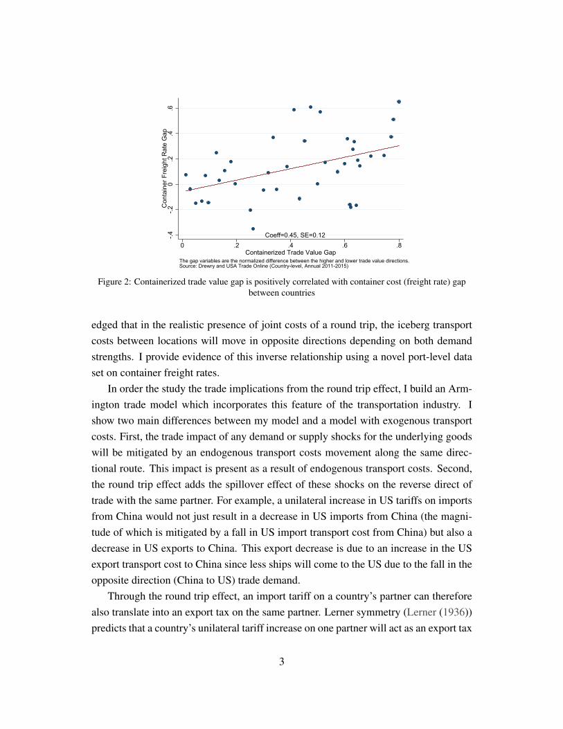
As a result, asymmetric demand between locations translates into asymmetric trans-port costs. China runs a large trade surplus with the United States, and the cost to shipa container from China to the US ($1900 per container) is more than three times thereturn cost ($600 per container).1 The US and UK, who have relatively more balancedtrade with each other, have more similar container costs ($1300 per container from UKto US compared to the return cost of $1000 per container). Not just unique to containershipping, the round trip effect also applies to air cargo and US domestic trucking.2 Fig-ure 2 shows that the gap in containerized trade value to and from a pair of countries,which approximates the trade demand asymmetry between countries, is positively cor-related with the gap in the cost of containers going to and from these countries. Thisrelationship can also be established with container volumes (figure A.1).

12013 container freight rates from Drewry Maritime Research.2The cost to ship air cargo from China to US is ten times more than the return cost ($3-$3.50 per kg

from China to US compared to 30-40 cents per kg on the return; Behrens and Picard (2011)). Withinthe US domestically, it costs two times more to rent a truck from Chicago to Philadelphia than the return($1963 at $2.69 per mile from Chicago to Philadelphia compared to $993 at $1.31 per mile for the return;DAT Solutions).

1

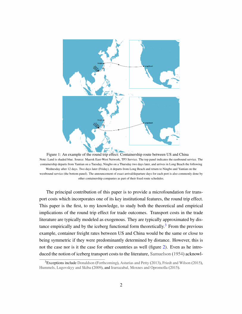
Figure 1: An example of the round trip effect: Containership route between US and ChinaNote: Land is shaded blue. Source: Maersk East-West Network, TP3 Service. The top panel indicates the eastbound service. Thecontainership departs from Yantian on a Tuesday, Ningbo on a Thursday two days later, and arrives in Long Beach the following

Wednesday after 12 days. Two days later (Friday), it departs from Long Beach and return to Ningbo and Yantian on thewestbound service (the bottom panel). The announcement of exact arrival/departure days for each port is also commonly done by

other containership companies as part of their fixed route schedules.

The principal contribution of this paper is to provide a microfoundation for trans-port costs which incorporates one of its key institutional features, the round trip effect.This paper is the first, to my knowledge, to study both the theoretical and empiricalimplications of the round trip effect for trade outcomes. Transport costs in the tradeliterature are typically modeled as exogenous. They are typically approximated by dis-tance empirically and by the iceberg functional form theoretically.3 From the previousexample, container freight rates between US and China would be the same or close tobeing symmetric if they were predominantly determined by distance. However, this isnot the case nor is it the case for other countries as well (figure 2). Even as he intro-duced the notion of iceberg transport costs to the literature, Samuelson (1954) acknowl-

3Exceptions include Donaldson (Forthcoming), Asturias and Petty (2013), Friedt and Wilson (2015),Hummels, Lugovskyy and Skiba (2009), and Irarrazabal, Moxnes and Opromolla (2015).

2

Coeff=0.45, SE=0.12-.4-.2

0.2

.4.6

Con

tain

er F

reig

ht R

ate

Gap

0 .2 .4 .6 .8Containerized Trade Value Gap

The gap variables are the normalized difference between the higher and lower trade value directions.Source: Drewry and USA Trade Online (Country-level, Annual 2011-2015)

Figure 2: Containerized trade value gap is positively correlated with container cost (freight rate) gapbetween countries

edged that in the realistic presence of joint costs of a round trip, the iceberg transportcosts between locations will move in opposite directions depending on both demandstrengths. I provide evidence of this inverse relationship using a novel port-level dataset on container freight rates.

In order the study the trade implications from the round trip effect, I build an Arm-ington trade model which incorporates this feature of the transportation industry. Ishow two main differences between my model and a model with exogenous transportcosts. First, the trade impact of any demand or supply shocks for the underlying goodswill be mitigated by an endogenous transport costs movement along the same direc-tional route. This impact is present as a result of endogenous transport costs. Second,the round trip effect adds the spillover effect of these shocks on the reverse direct oftrade with the same partner. For example, a unilateral increase in US tariffs on importsfrom China would not just result in a decrease in US imports from China (the magni-tude of which is mitigated by a fall in US import transport cost from China) but also adecrease in US exports to China. This export decrease is due to an increase in the USexport transport cost to China since less ships will come to the US due to the fall in theopposite direction (China to US) trade demand.

Through the round trip effect, an import tariff on a country’s partner can thereforealso translate into an export tax on the same partner. Lerner symmetry (Lerner (1936))predicts that a country’s unilateral tariff increase on one partner will act as an export tax

3

and reduce its exports to all its partners due to the balanced trade condition in a generalequilibrium setting. I present a specific bilateral channel that impacts the country’sexports to the same partner within a partial equilibrium framework, without requiringthe balanced trade condition.4

I provide suggestive evidence for two main predictions from my trade and trans-port model using a proprietary data set on port-level container freight rates matched tocontainerized trade data. First, freight rates within port pairs are negatively correlatedacross time and within routes. This inverse relationship is predicted in my model dueto transport firms optimizing over a round trip. As such, the transport costs in eachdirection of the port pair route will move in opposing directions in response to demandchanges across time. If freight rates were independently determined in each direction ofa port pair, one would expect there to be no correlation. In addition, if freight rates weremostly determined by distance, one would also expect no correlation since route fixedeffects are included in my regressions. Second, outgoing containerized trade value ispositively correlated with incoming freight rates across time and within dyads. Thisapplies to incoming trade value and outgoing freight rates as well. This relationshipwould not be present if there was no systematic linkage between aggregate outgoingcontainerized trade value and the incoming freight rates. The round trip effect providesone such explanation.

Next, I estimate the containerized trade elasticity with respect to freight rates usingthe round trip insight. Since containers are required to transport containerized trade,this elasticity can also be interpreted as the demand elasticity for containers. In typicaldemand estimations, I require a transport supply shifter that is independent of demanddeterminants. In the example of estimating containerized trade demand from UK to US,I need a shifter of transport supply from UK to US that is independent of the demanddeterminants on the same route. I develop a novel supply shifter utilizing the roundtrip effect: shocks which affect the opposite direction containerized trade (from USto UK). These shocks will shift both its own container transport supply as well as thetransport supply in the original direction (from UK to US). This latter transport supplyshift will identify the containerized trade demand from UK to the US if the demandshocks between routes are uncorrelated. Since demand shifts between countries aregenerally not independent, I construct a Bartik shift-share instrument that appromixates

4My findings are in line with Costinot and Werning (2017) who show that trade balance is not anecessary or sufficient condition for the Lerner Symmetry to hold.

4

this transport supply shift. I find that a one percent increase in container freight ratesleads to a 2.8 percent decrease in containerized trade value, 3.6 percent decrease intrade weight, and a 0.8 percent increase in trade value per weight. Since trade valueper weight can be interpreted as a rough measure of trade quality, my third result is inline with the positive link between quality and per unit trade costs first established byAlchian and Allen (1964).

Using my trade elasticity estimated from the instrumental variable approach, I esti-mate parameters in my transportation and trade model by matching the observed freightrate and trade data. I then simulate a counterfactual in which US doubles its tariffs onall its partners from an overall trade weighted average of 1.16 percent. I show that therise in the US tariff will both decrease US imports from these partners and decrease USexports to these partners. I show that the same model with exogenous transport costswould over-predict the average import decrease by 41 percent, not predict any exportdecrease, and under-predict the total trade changes by an average of 25 percent. Over-all, increasing US import tariffs by a factor of one will result in a constant 0.2 percenttax on export prices.

This paper contributes to several strands of literature. First, it is broadly related tothe literature which studies how trade costs affect trade flow between countries (Ander-son and Van Wincoop (2004), Eaton and Kortum (2002), as well as Head and Mayer(2014)). In particular, I focus on the literature on transport cost (Hummels (2007) andLimao and Venables (2001)) and highlight a feature of the transportation industry—the round trip effect—using a novel high frequency data set on bilateral freight rates.Previous theoretical studies on the round trip effect investigates how it affects the spa-tial distribution of firms (Behrens and Picard (2011)) and the potential harmful impactfrom domestic import restrictions on exports (Ishikawa and Tarui (2016)). The theorymodel in this paper builds on Behrens and Picard (2011). Previous empirical studies onthe round trip effect typically employs aggregate data sets at the regional level (Friedtand Wilson (2015)) or within a country at the annual frequency (Tanaka and Tsubota(2016) and Jonkeren et al. (2011))5. My data is at the monthly frequency, the port-levelin both directions, and includes the largest ports globally. This high level of disaggre-

5Tanaka and Tsubota (2016) estimates the effects of trade flow imbalance on transport price ratiobetween Japanese prefectures. Focusing on 3 regions (US, Asia, and Europe), Friedt and Wilson (2015)evaluate the impact of freight rates on dominant and secondary routes. Jonkeren et al. (2011) focuses ondry bulk cargo in the inland waterways of the Rhine. Friedt (2017) studies the impact of commercial andenvironmental policy on US-EU bilateral trade flows in the presence of the round trip effect.

5

gation allows me to better study the round trip effect and its trade implications. I amalso able to exploit the panel nature of this data set in my empirical estimations.

Second, this paper develops a novel IV strategy using an institutional detail of thetransportation industry in order to estimate a transport mode-specific trade elasticitywith respect to transport cost. This is the first paper to do so. Previous studies havetypically focused on trade elasticities across all transport modes (e.g. Head and Mayer(2014), Shapiro (2015)) and my elasticity contributes to understanding how trade elas-ticities respond to transport costs within a mode, i.e. container shipping. Additionally,the round trip effect applies to the transportation industries servicing both internationaland domestic trade. As such, endogenous transport costs may have an important con-tribution to the spatial allocation of production in and across countries. My IV strategycan be utilized to identify this.

This paper is also related to empirical literature on endogenous transport costs. Mytheory model builds on Hummels, Lugovskyy and Skiba (2009) by introducing theround trip effect feature in the transport firms framework. Hummels, Lugovskyy andSkiba (2009) investigates the role of market power on transport prices using US andLatin American imports data.6 Focusing on dry bulk ships, Brancaccio, Kalouptsidiand Papageorgiou (2017) studies endogenous transport costs in the presence of searchfrictions between exporters and transport firms. Hummels and Skiba (2004) investi-gates the relationship between per unit trade cost and product prices. Third, this paperis related to studies on containerization and trade. Cosar and Pakel (2017) studies theeffects of containerization on transport by looking at the choice between containeriza-tion and breakbulk shipping. Bernhofen, El-Sahli and Kneller (2016) estimates theeffects of containerization on world trade while Rua (2014) investigates the diffusionof containerization.

In the next section, I incorporate a transportation market into an Armington model.I present the comparative statics from trade shocks in my model and compare them tooutcomes from an exogenous transport cost model. In section 3, I introduce my noveldata set on port-level container freight rates matched to containerized trade data andestablish suggestive evidence for two predictions in my theory model. I develop aninstrument based on the round trip effect insight in section 4 to address endogeneitybetween transport cost and trade. I highlight my results in section 5. In section 6, I

6Other studies that focus on market power within the transport sector include Asturias and Petty(2013) and Francois and Wooton (2001).

6

utilize my trade elasticity from section 5 to estimate parameters in my theory modelin section 2 in order to match the observed trade and freight rates data. I then sim-ulate a counterfactual increase in US import tariffs on all its partners. I compare thetrade predictions from my model to a model with exogenous transport cost. Section 7concludes.

2 Theoretical FrameworkThis section presents the theoretical implications of endogenous transport costs and

the round trip effect in an Armington trade model. To highlight the impact of the roundtrip effect on the model, I start by solving the model under the assumption that transportcosts are exogenous and then incorporate a transport sector with the round trip effect.I then describe the comparative statics between the two models. Appendix sectionA.1 presents a graphical illustration of the round trip effect and its mechanism using asimple linear transport demand and supply model.

The trade model in this paper is a modification of Hummels, Lugovskyy and Skiba(2009) to incorporate the round trip effect and to allow for heterogeneous countries. Tomaintain simplicity in a first pass of modeling the round trip effect, I assume perfectlycompetitive transport firms. The main results here do not hinge on this assumption.

2.1 Model SetupThe world consists of j = 1,2, ...M potentially heterogeneous countries where each

country produces a different variety of a tradeable good. Consumers consume all va-rieties of this tradeable good from all countries as well as a homogeneous numerairegood. The utility function of a representative consumer in country j is quasilinear:

U j = q j0 +M

∑i=1

ai jq(σ−1)/σ

i j , σ > 1 (1)

where q j0 is the quantity of the numeraire good consumed by country j, ai j is j’spreference parameter for the variety from country i, qi j the quantity of variety from iconsumed j, while σ is the price elasticity of demand. The numeraire good is costlesslytraded and its price is normalized to one.

Assuming that each country is perfectly competitive in producing their variety andthat labor is the only input to production, the delivered price of country i’s good in j(pi j) reflects its delivered cost which includes i’s domestic wages (wi), the ad-valorem

7

tariff rate that j imposes on i (τi j ≥ 1), and a per unit transport cost (Ti j):

pi j = wiτi j +Ti j (2)

2.2 Exogenous transport cost modelThe cost of transport here is an exogenously determined one-way marginal cost of

shipping (ci j). The delivered price of country i’s good in j (pExoi j ) is then:

pExoi j = wiτi j + ci j (3)

An increase in the marginal cost of transport (ci j), j’s tariff on i (τi j), or wages in i(wi) will increase the equilibrium price of i’s good in country j. Following Behrensand Picard (2011) and Hummels, Lugovskyy and Skiba (2009), one unit of transportservices is required to ship one unit of good.

The utility-maximizing quantity of i’s good consumed in j (qExoi j ) is derived from

the condition that the price ratio of i’s good relative to the numeraire is equal to themarginal utility ratio of that good relative to the numeraire.7 The equilibrium tradevalue of i’s good in j (XExo

i j ) is the product of the delivered price (pExoi j ) and quantity

(qExoi j ) on route i j:

qExoi j =

[σ

σ −11

ai j

(wiτi j + ci j

)]−σ

XExoi j ≡ pExo

i j qExoi j =

[σ

σ −11

ai j

]−σ [(wiτi j + ci j

)]1−σ

(4)

An increase in j’s preference for i’s good (ai j) will increase both the equilibrium quan-tity and value. On the other hand, an increase in i’s wages, j’s import tariff on i, andthe transport marginal cost will decrease both.

2.3 Endogenous transport cost and the round trip effectHere transportation is endogenized with the round trip effect. The profit function

of a perfectly competitive transport firm servicing the round trip between i and j (π←→i j )

7From equation (4), σ is the price elasticity of demand: ∂qExoi j

∂ pExoi j

qExoi j

pExoi j

= −σ . This equilibrium quantitydiffers from a standard CES demand because it is relative to the numeraire rather than relative to a bundleof the other varieties. If this model is not specified with a numeraire good, this quantity expression wouldinclude a CES price index that is specific to each country (in this case country j). I follow Hummels,Lugovskyy and Skiba (2009) in controlling for importer fixed effects in my empirical estimates. Thisfixed effect can be interpreted as the price of the numeraire good or as the CES price index in the morestandard non-numeraire case. Stemming from this, the balanced trade condition between countries issatisfied by the numeraire good.

8

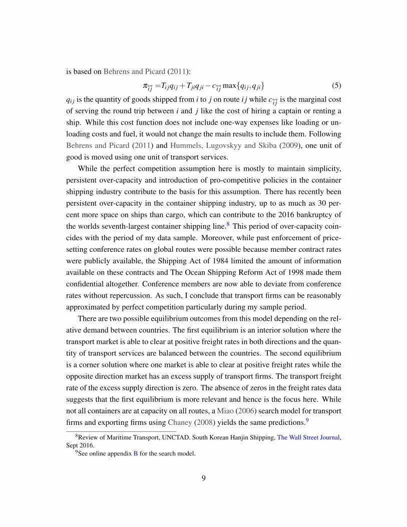
is based on Behrens and Picard (2011):

π←→i j =Ti jqi j +Tjiq ji− c←→i j max{qi j,q ji} (5)

qi j is the quantity of goods shipped from i to j on route i j while c←→i j is the marginal costof serving the round trip between i and j like the cost of hiring a captain or renting aship. While this cost function does not include one-way expenses like loading or un-loading costs and fuel, it would not change the main results to include them. FollowingBehrens and Picard (2011) and Hummels, Lugovskyy and Skiba (2009), one unit ofgood is moved using one unit of transport services.

While the perfect competition assumption here is mostly to maintain simplicity,persistent over-capacity and introduction of pro-competitive policies in the containershipping industry contribute to the basis for this assumption. There has recently beenpersistent over-capacity in the container shipping industry, up to as much as 30 per-cent more space on ships than cargo, which can contribute to the 2016 bankruptcy ofthe worlds seventh-largest container shipping line.8 This period of over-capacity coin-cides with the period of my data sample. Moreover, while past enforcement of price-setting conference rates on global routes were possible because member contract rateswere publicly available, the Shipping Act of 1984 limited the amount of informationavailable on these contracts and The Ocean Shipping Reform Act of 1998 made themconfidential altogether. Conference members are now able to deviate from conferencerates without repercussion. As such, I conclude that transport firms can be reasonablyapproximated by perfect competition particularly during my sample period.

There are two possible equilibrium outcomes from this model depending on the rel-ative demand between countries. The first equilibrium is an interior solution where thetransport market is able to clear at positive freight rates in both directions and the quan-tity of transport services are balanced between the countries. The second equilibriumis a corner solution where one market is able to clear at positive freight rates while theopposite direction market has an excess supply of transport firms. The transport freightrate of the excess supply direction is zero. The absence of zeros in the freight rates datasuggests that the first equilibrium is more relevant and hence is the focus here. Whilenot all containers are at capacity on all routes, a Miao (2006) search model for transportfirms and exporting firms using Chaney (2008) yields the same predictions.9

8Review of Maritime Transport, UNCTAD. South Korean Hanjin Shipping, The Wall Street Journal,Sept 2016.

9See online appendix B for the search model.

9

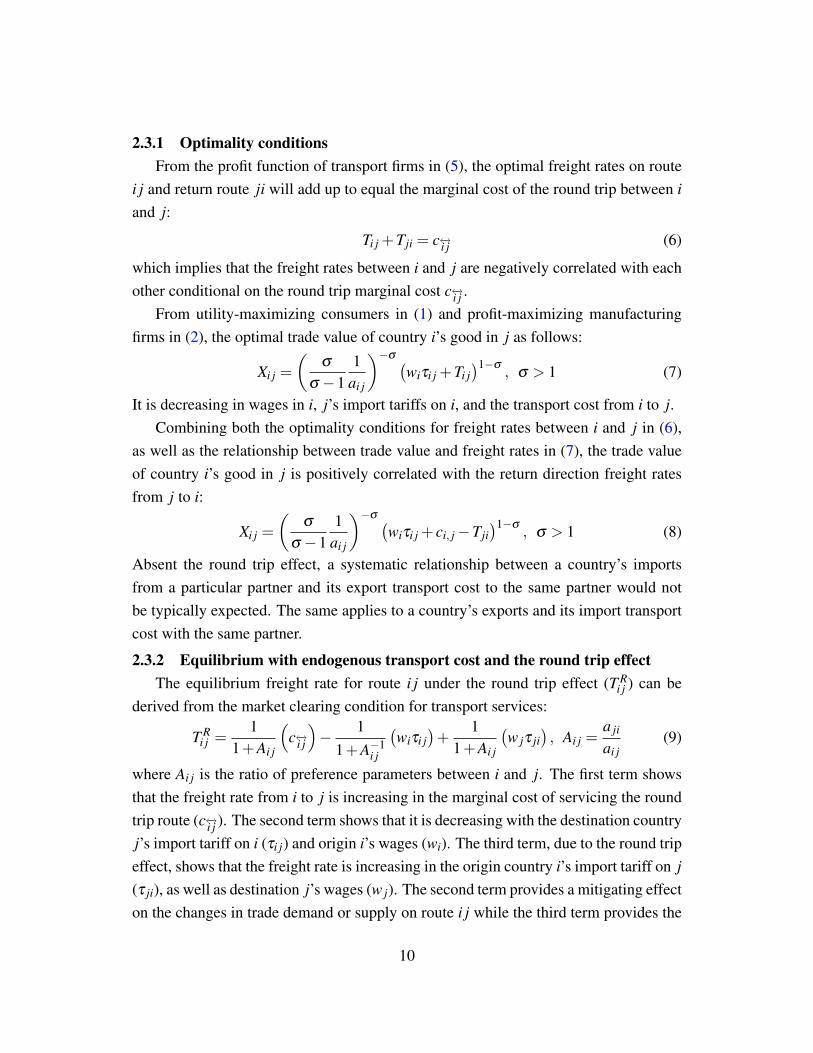
2.3.1 Optimality conditionsFrom the profit function of transport firms in (5), the optimal freight rates on route

i j and return route ji will add up to equal the marginal cost of the round trip between iand j:

Ti j +Tji = c←→i j (6)

which implies that the freight rates between i and j are negatively correlated with eachother conditional on the round trip marginal cost c←→i j .

From utility-maximizing consumers in (1) and profit-maximizing manufacturingfirms in (2), the optimal trade value of country i’s good in j as follows:

Xi j =

(σ

σ −11

ai j

)−σ (wiτi j +Ti j

)1−σ, σ > 1 (7)

It is decreasing in wages in i, j’s import tariffs on i, and the transport cost from i to j.Combining both the optimality conditions for freight rates between i and j in (6),

as well as the relationship between trade value and freight rates in (7), the trade valueof country i’s good in j is positively correlated with the return direction freight ratesfrom j to i:

Xi j =

(σ

σ −11

ai j

)−σ (wiτi j + ci, j−Tji

)1−σ, σ > 1 (8)

Absent the round trip effect, a systematic relationship between a country’s importsfrom a particular partner and its export transport cost to the same partner would notbe typically expected. The same applies to a country’s exports and its import transportcost with the same partner.

2.3.2 Equilibrium with endogenous transport cost and the round trip effectThe equilibrium freight rate for route i j under the round trip effect (T R

i j ) can bederived from the market clearing condition for transport services:

T Ri j =

11+Ai j

(c←→i j

)− 1

1+A−1i j

(wiτi j

)+

11+Ai j

(w jτ ji

), Ai j =

a ji

ai j(9)

where Ai j is the ratio of preference parameters between i and j. The first term showsthat the freight rate from i to j is increasing in the marginal cost of servicing the roundtrip route (c←→i j ). The second term shows that it is decreasing with the destination countryj’s import tariff on i (τi j) and origin i’s wages (wi). The third term, due to the round tripeffect, shows that the freight rate is increasing in the origin country i’s import tariff on j(τ ji), as well as destination j’s wages (w j). The second term provides a mitigating effecton the changes in trade demand or supply on route i j while the third term provides the

10

same mitigating effect but for changes on the opposite route ji.10

The equilibrium price of country i’s good in j is increasing in the marginal cost ofround trip transport c←→i j , as well as the wages and import tariffs in both countries. Thisprice is a function of j’s own wages and the import tariff it faces from i is due to theround trip effect:

pRi j =

11+Ai j

(w jτ ji +wiτi j + c←→i j

), Ai j =

a ji

ai j(10)

The equilibrium trade quantity and value on route i j are decreasing in the marginalcost of transport, both countries’ wages and import tariffs:11

qRi j =

[σ

σ −11

ai j

11+Ai j

(w jτ ji +wiτi j + c←→i j

)]−σ

XRi j =

[σ

σ −11

ai j

]−σ [ 11+Ai j

(w jτ ji +wiτi j + c←→i j

)]1−σ

, Ai j =a ji

ai j

(11)

These equilibrium outcomes are due to the round trip effect: a country’s imports andexports to a particular trading partner are linked through transportation. For example,when country i increases its import tariff on country j (τ ji), not only will its own importsfrom j be affected, but its exports to j as well (equation (11)). The comparative staticssection below elaborates.

2.4 Comparative staticsThis subsection describes the trade predictions from changes in import tariffs and

preferences between both models. When country j’s import tariff on country i (τi j)increases, an exogenous transport cost model will predict only changes in j’s importsfrom i. The price of j’s imports from i will become more expensive (equation (3))while its import quantity and value from i will fall (equation (4)).

When transport cost is endogenized with the round trip effect, however, j’s importtariff increase will affect both j’s imports from and exports to i. This is due to theendogenous response from j’s imports and export freight rates to i. First, country j’simport freight rate will fall to mitigate the impact of the tariff (equation (9)). Thisdecrease is not enough to offset j’s net import price increase from i (equation (10))which results in a fall in j’s import quantity and value (equation (11)). This import fall,

10If countries are symmetric, the preference parameters would be the same: ai j = a ji. The freight rateseach way will be half the marginal cost: T Sym

i j = T Symji = 1

2 c←→i j . See theory appendix A.2 for more details.11If countries are symmetric, they face the same prices, quantities, and values. See theory appendix

A.2.

11

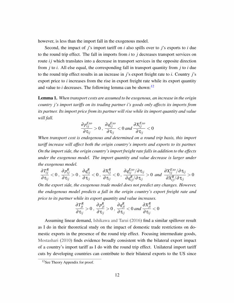
however, is less than the import fall in the exogenous model.Second, the impact of j’s import tariff on i also spills over to j’s exports to i due

to the round trip effect. The fall in imports from i to j decreases transport services onroute i j which translates into a decrease in transport services in the opposite directionfrom j to i. All else equal, the corresponding fall in transport quantity from j to i dueto the round trip effect results in an increase in j’s export freight rate to i. Country j’sexport price to i increases from the rise in export freight rate while its export quantityand value to i decreases. The following lemma can be shown:12

Lemma 1. When transport costs are assumed to be exogenous, an increase in the origincountry j’s import tariffs on its trading partner i’s goods only affects its imports fromits partner. Its import price from its partner will rise while its import quantity and valuewill fall.

∂ pExoi j

∂τi j> 0 ,

∂qExoi j

∂τi j< 0 and

∂XExoi j

∂τi j< 0

When transport cost is endogenous and determined on a round trip basis, this importtariff increase will affect both the origin country’s imports and exports to its partner.On the import side, the origin country’s import freight rate falls in addition to the effectsunder the exogenous model. The import quantity and value decrease is larger underthe exogenous model.

∂T Ri j

∂τi j< 0 ,

∂ pRi j

∂τi j> 0 ,

∂qRi j

∂τi j< 0 ,

∂XRi j

∂τi j< 0 ,

∂qExoi j /∂τi j

∂qRi j/∂τi j

> 0 and∂XExo

i j /∂τi j

∂XRi j/∂τi j

> 0

On the export side, the exogenous trade model does not predict any changes. However,the endogenous model predicts a fall in the origin country’s export freight rate andprice to its partner while its export quantity and value increases.

∂T Rji

∂τi j> 0 ,

∂ pRji

∂τi j> 0 ,

∂qRji

∂τi j< 0 and

∂XRji

∂τi j< 0

Assuming linear demand, Ishikawa and Tarui (2016) find a similar spillover resultas I do in their theoretical study on the impact of domestic trade restrictions on do-mestic exports in the presence of the round trip effect. Focusing intermediate goods,Mostashari (2010) finds evidence broadly consistent with the bilateral export impactof a country’s import tariff as I do with the round trip effect. Unilateral import tariffcuts by developing countries can contribute to their bilateral exports to the US since

12See Theory Appendix for proof.

12

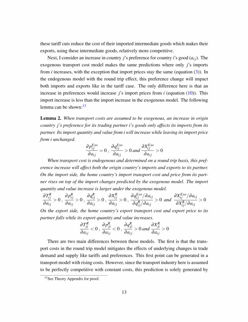
these tariff cuts reduce the cost of their imported intermediate goods which makes theirexports, using these intermediate goods, relatively more competitive.

Next, I consider an increase in country j’s preference for country i’s good (ai j). Theexogenous transport cost model makes the same predictions where only j’s importsfrom i increases, with the exception that import prices stay the same (equation (3)). Inthe endogenous model with the round trip effect, this preference change will impactboth imports and exports like in the tariff case. The only difference here is that anincrease in preferences would increase j’s import prices from i (equation (10)). Thisimport increase is less than the import increase in the exogenous model. The followinglemma can be shown:13

Lemma 2. When transport costs are assumed to be exogenous, an increase in origincountry j’s preference for its trading partner i’s goods only affects its imports from itspartner. Its import quantity and value from i will increase while leaving its import pricefrom i unchanged.

∂ pExoi j

∂ai j= 0 ,

∂qExoi j

∂ai j> 0 and

∂XExoi j

∂ai j> 0

When transport cost is endogenous and determined on a round trip basis, this pref-erence increase will affect both the origin country’s imports and exports to its partner.On the import side, the home country’s import transport cost and price from its part-ner rises on top of the import changes predicted by the exogenous model. The importquantity and value increase is larger under the exogenous model.

∂T Ri j

∂ai j> 0 ,

∂ pRi j

∂ai j> 0 ,

∂qRi j

∂ai j> 0 ,

∂XRi j

∂ai j> 0 ,

∂qExoi j /∂ai j

∂qRi j/∂ai j

> 0 and∂XExo

i j /∂ai j

∂XRi j/∂ai j

> 0

On the export side, the home country’s export transport cost and export price to itspartner falls while its export quantity and value increases.

∂T Rji

∂ai j< 0 ,

∂ pRji

∂ai j< 0 ,

∂qRji

∂ai j> 0 and

∂XRji

∂ai j> 0

There are two main differences between these models. The first is that the trans-port costs in the round trip model mitigates the effects of underlying changes in tradedemand and supply like tariffs and preferences. This first point can be generated in atransport model with rising costs. However, since the transport industry here is assumedto be perfectly competitive with constant costs, this prediction is solely generated by

13See Theory Appendix for proof.

13

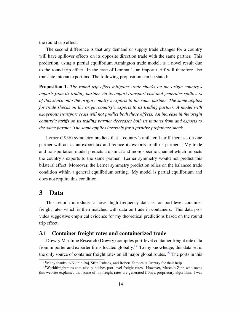
the round trip effect.The second difference is that any demand or supply trade changes for a country

will have spillover effects on its opposite direction trade with the same partner. Thisprediction, using a partial equilibrium Armington trade model, is a novel result dueto the round trip effect. In the case of Lemma 1, an import tariff will therefore alsotranslate into an export tax. The following proposition can be stated:

Proposition 1. The round trip effect mitigates trade shocks on the origin country’simports from its trading partner via its import transport cost and generates spilloversof this shock onto the origin country’s exports to the same partner. The same appliesfor trade shocks on the origin country’s exports to its trading partner. A model withexogenous transport costs will not predict both these effects. An increase in the origincountry’s tariffs on its trading partner decreases both its imports from and exports tothe same partner. The same applies inversely for a positive preference shock.

Lerner (1936) symmetry predicts that a country’s unilateral tariff increase on onepartner will act as an export tax and reduce its exports to all its partners. My tradeand transportation model predicts a distinct and more specific channel which impactsthe country’s exports to the same partner. Lerner symmetry would not predict thisbilateral effect. Moreover, the Lerner symmetry prediction relies on the balanced tradecondition within a general equilibrium setting. My model is partial equilibrium anddoes not require this condition.

3 DataThis section introduces a novel high frequency data set on port-level container

freight rates which is then matched with data on trade in containers. This data pro-vides suggestive empirical evidence for my theoretical predictions based on the roundtrip effect.

3.1 Container freight rates and containerized tradeDrewry Maritime Research (Drewry) compiles port-level container freight rate data

from importer and exporter firms located globally.14 To my knowledge, this data set isthe only source of container freight rates on all major global routes.15 The ports in this

14Many thanks to Nidhin Raj, Stijn Rubens, and Robert Zamora at Drewry for their help.15Worldfreightrates.com also publishes port-level freight rates. However, Marcelo Zinn who owns

this website explained that some of his freight rates are generated from a proprietary algorithm. I was

14

data set are the biggest globally and handle more than one million containers per year.These monthly or bimonthly spot market rates are for a standard 20-foot container.

In addition to spot market rates, long-term contracts are also used in the containermarket. My spot rates choice is driven by data availability. Contract rates are con-fidentially filed with the Federal Maritime Commission (FMC) and my Freedom ofInformation Act requests have been denied.16 That being said, spot prices play animportant role in informing long-term contracts and can shed light on the containertransport market. Shorter-term contracts are increasingly favored due to over-capacityin the market (conversations with Director of FMC Office of Economics & Competi-tion Analysis, Roy Pearson). Longer term contracts are also increasingly indexed tospot market rates due to price fluctuations (Journal of Commerce, January 2014). Fur-thermore, most firms split their cargo between long-term contracts and the spot marketto smooth volatility (conversations with Roy Pearson). Freight forwarding companieslike UPS or FedEx offer hybird models that allow their customers to switch to spot ratepricing when these rates fall below agreed-upon contract rates (Journal of Commerce,June 2016).

While containers carry the two-thirds of world trade by value (World ShippingCouncil), they do not carry all types of products. Cars and oil, for example, are nottransported via containers. As such, in order to compare apples to apples, I focus myanalysis on trade in containers. Since containerized trade data is not readily availablefor all other countries apart from the United States, my analysis is limited to US tradein this paper. Drewry collects freight-rate data on the three of the largest US containerports (Los Angeles and Long Beach, New York, and Houston) that handle 16.7 mil-lion containers annually combined—more than half of the annual US container volume(MARAD). There are 68 port pairs which include these three US ports.

Monthly containerized US trade data at the port level is available from USA TradeOnline at the six-digit Harmonized System (HS) product code level. It includes thetrade value and weight between US ports and its foreign partner countries.17 My levelof observation is at the US port, foreign partner country, and product level, but for easeof exposition I will refer to both destination and origin locations as a country. Both

not able to ascertain the proportion of real versus generated data from Mr. Zinn. Drewry’s data reflectsthe actual prices paid.

16For more details, refer to the Data Appendix.17Since my freight rates data is at the port-to-port level, I have to aggregate my data to the US port

and foreign country level. See Data Appendix for further details.

15

freight rates and trade value data are converted into real terms. Containerized tradeaccount for 62% of all US vessel trade value in 2015.18 My matched freight rates andtrade data set represents at least half of total US containerized trade value in 2014 (USATrade Online).19 The time period of this matched data set is from January 2011 to June2016.

3.2 Summary StatisticsTable 1 shows the summary statistics for US freight rates, as well as containerized

trade value, weight, and value per weight. As a first pass, this data set is broken downby US exports, US imports, and total US trade. These variables are on average higheron for US imports than exports. While the higher import values and weight are notsurprising since US is a net-importer, freight rates are also higher for US imports thanexports. The value per weight of US imports, a crude measure of quality, is on averagehigher than US exports. These patterns are also affirmed using more aggregate data oncontainer volumes (table A.1). After converting per unit freight rates into ad valoremequivalents, US iceberg cost are also higher for imports (table A.1). However, ice-berg costs belie two endogenous components: freight rates and trade value. Containerfreight rates and containerized trade value are jointly determined since they are marketoutcomes. This paper will study them as such.

The summary statistics in table 1 affirms the “shipping the good apples out” phe-nomenon first introduced by Alchian and Allen (1964) and extended by Hummels andSkiba (2004)–the presence of per unit transportation costs lowers the relative price ofhigher-quality goods. Table 1 shows the presence of higher US import freight rates aswell as higher import value per weight relative to exports. Similarly, table A.1 showsthat the value per container for imports are higher than exports as well.

3.3 Suggestive EvidenceMy novel data set on container freight rates, matched with containerized trade data,

is uniquely positioned to provide suggestive evidence for my theoretical predictionsfrom the previous section. The first suggestive evidence is as follows:

Suggestive Evidence 1. A positive deviation from the average freight rates from i to j

18Shipping vessels that carry trade without containers include oil tankers, bulk carriers, and car carri-ers. Bulk carriers transport grains, coal, ore, and cement.

19This is a conservative estimate, particularly for Europe, since Drewry does not collect data on adja-cent ports even though they are in different countries. See the Data Appendix for more details.

16

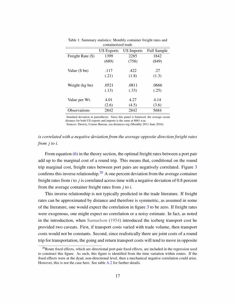
Table 1: Summary statistics: Monthly container freight rates andcontainerized trade

US Exports US Imports Full SampleFreight Rate ($) 1399 2285 1842

(689) (758) (849)

Value ($ bn) .117 .422 .27(.21) (1.8) (1.3)

Weight (kg bn) .0521 .0811 .0666(.13) (.33) (.25)

Value per Wt. 4.01 4.27 4.14(2.6) (4.5) (3.6)

Observations 2842 2842 5684Standard deviation in parentheses. Since this panel is balanced, the average ocean

distance for both US exports and imports is the same at 8061 n.m.Sources: Drewry, Census Bureau, sea-distances.org (Monthly 2011-June 2016).

is correlated with a negative deviation from the average opposite direction freight ratesfrom j to i.

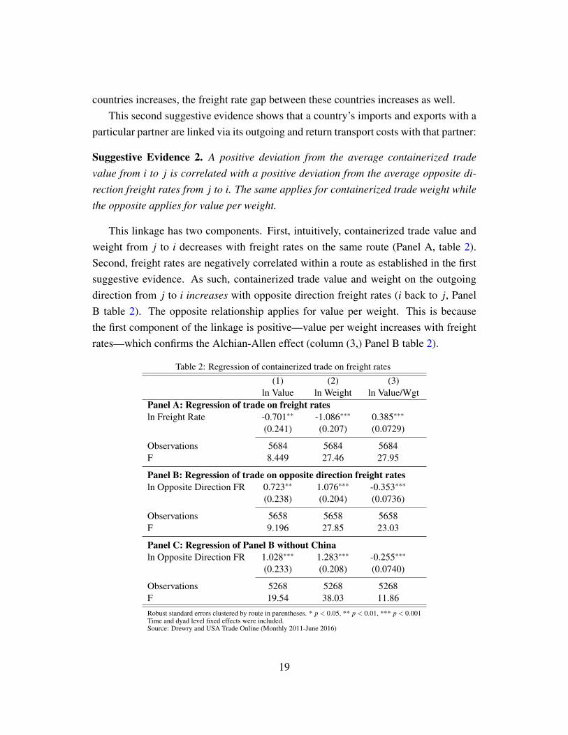
From equation (6) in the theory section, the optimal freight rates between a port pairadd up to the marginal cost of a round trip. This means that, conditional on the roundtrip marginal cost, freight rates between port pairs are negatively correlated. Figure 3confirms this inverse relationship.20 A one percent deviation from the average containerfreight rates from i to j is correlated across time with a negative deviation of 0.8 percentfrom the average container freight rates from j to i.

This inverse relationship is not typically predicted in the trade literature. If freightrates can be approximated by distance and therefore is symmetric, as assumed in someof the literature, one would expect the correlation in figure 3 to be zero. If freight rateswere exogenous, one might expect no correlation or a noisy estimate. In fact, as notedin the introduction, when Samuelson (1954) introduced the iceberg transport cost heprovided two caveats. First, if transport costs varied with trade volume, then transportcosts would not be constants. Second, since realistically there are joint costs of a roundtrip for transportation, the going and return transport costs will tend to move in opposite

20Route fixed effects, which are directional port-pair fixed effects, are included in the regression usedto construct this figure. As such, this figure is identified from the time variation within routes. If thefixed effects were at the dyad, non-directional level, then a mechanical negative correlation could arise.However, this is not the case here. See table A.2 for further details.

17

Coef=-0.82, Robust SE=0.020.6

1.1

1.8

3.0

ln C

onta

iner

Fre

ight

Rat

es (T

dol

lars

)

0.6 1.1 1.8 3.0ln Container Freight Rates on Opposite Direction Route (T dollars)

Robust standard errors clustered by route with time and route controls.Source: Drewry and USA Trade Online (Monthly 2011-June 2016)

Figure 3: Correlation between container freight rates within port pairslnTi jt = β0 +β1 lnTjit +di j + γt + εi jt

directions depending on the demand levels.21 I confirm his caveats here.Furthermore, the presence of this inverse relationship means that container routes

can generally be represented by the port-pairs in my data. One contributing reasonfor this is the significant increase in average container ship sizes—container-carryingcapacity has increased by about 1200% since 1970 (Container ship design, World Ship-ping Council). The increase in average ship size has resulted in downward pressure onthe average number of port calls per route because larger ships face greater number ofhours lost at port. Ducruet and Notteboom (2012) shows that the number of Europeanport calls per loop on the Far East-North Europe trade has decreased from 4.9 portsof call in 1989 down to 3.35 in December 2009. Second, this size increase has alsogenerated a proliferation of hub-and-spoke networks which also decreases the numberof port calls per route: 85 percent of container shipping networks are of the hub-and-spoke form (Rodrigue, Comtois and Slack (2013)) and 81 percent of country pairs areconnected by one transhipment port or less (Fugazza and Hoffmann (2016)).

The round trip effect can be also shown using container quantities directly. FigureA.1 highlights a positive relationship between container volume gap and freight rategap between countries. As the number of containers going back and forth between

21Systematic current and wind conditions can contribute to this inverse relationship. Chang et al.(2013) estimates a modest range of 1 to 8 percent in time savings when ships utilize strong currents oravoid unfavorable currents in the North Pacific. As such, the highly negative and significant relationshipin figure 3 is not solely driven by currents.

18

countries increases, the freight rate gap between these countries increases as well.This second suggestive evidence shows that a country’s imports and exports with a

particular partner are linked via its outgoing and return transport costs with that partner:

Suggestive Evidence 2. A positive deviation from the average containerized tradevalue from i to j is correlated with a positive deviation from the average opposite di-rection freight rates from j to i. The same applies for containerized trade weight whilethe opposite applies for value per weight.

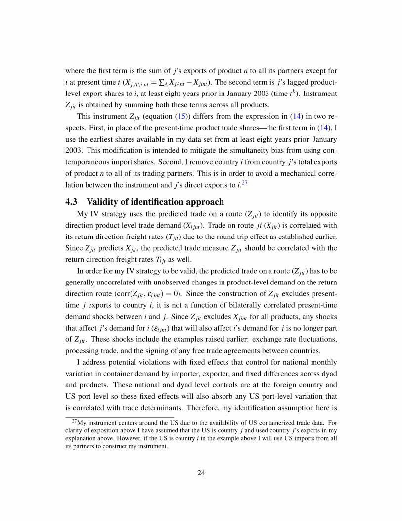
This linkage has two components. First, intuitively, containerized trade value andweight from j to i decreases with freight rates on the same route (Panel A, table 2).Second, freight rates are negatively correlated within a route as established in the firstsuggestive evidence. As such, containerized trade value and weight on the outgoingdirection from j to i increases with opposite direction freight rates (i back to j, PanelB table 2). The opposite relationship applies for value per weight. This is becausethe first component of the linkage is positive—value per weight increases with freightrates—which confirms the Alchian-Allen effect (column (3,) Panel B table 2).

Table 2: Regression of containerized trade on freight rates

(1) (2) (3)ln Value ln Weight ln Value/Wgt

Panel A: Regression of trade on freight ratesln Freight Rate -0.701∗∗ -1.086∗∗∗ 0.385∗∗∗

(0.241) (0.207) (0.0729)

Observations 5684 5684 5684F 8.449 27.46 27.95

Panel B: Regression of trade on opposite direction freight ratesln Opposite Direction FR 0.723∗∗ 1.076∗∗∗ -0.353∗∗∗

(0.238) (0.204) (0.0736)

Observations 5658 5658 5658F 9.196 27.85 23.03

Panel C: Regression of Panel B without Chinaln Opposite Direction FR 1.028∗∗∗ 1.283∗∗∗ -0.255∗∗∗

(0.233) (0.208) (0.0740)

Observations 5268 5268 5268F 19.54 38.03 11.86Robust standard errors clustered by route in parentheses. * p < 0.05, ** p < 0.01, *** p < 0.001Time and dyad level fixed effects were included.Source: Drewry and USA Trade Online (Monthly 2011-June 2016)

19

Specifically, within a port-pair dyad, a one percent deviation from the average op-posite direction freight rates (from i to j) is correlated across time with a 0.7 percentincrease in average aggregate containerized trade value in the going direction from j toi (column (1), Panel B table 2 and figure 4). In column (2), a within dyad one percentincrease from the average opposite direction freight rates is correlated across time witha 1.1 percent increase in average aggregate containerized trade weight in the going di-rection. Correspondingly in column (3), the value per weight on the outgoing directiondecreases with opposite direction freight rates. A within dyad one percent increase inthe average opposite direction freight rates (from j to i) is correlated across time witha 0.4 percent decrease in average aggregate containerized trade quality (from i to j).

Coeff=0.72 , Robust SE=0.214.7

24.2

39.8

65.7

ln C

onta

iner

ized

Tra

de V

alue

(M d

olla

rs)

0.7 1.1 1.8 3.0ln Return Direction Container Freight Rates (T dollars)

Robust standard errors clustered by route with time and dyad controls.Source: Drewry and USA Trade Online (Monthly 2011-June 2016)

Figure 4: Correlation between containerized trade value and opposite direction freight rateslnXi jt = β0 +β1 lnTjit +d↔

i j+ γt + εi jt

These findings suggest the presence of the round trip effect. Absent this effect,there should be no systematic relationship between containerized trade on the outgoingdirection and freight rates on the incoming direction. The same applies for trade onthe incoming direction and freight rates on the outgoing direction. While it is acknowl-edged here that the dominance of processing trade can also contribute to this relation-ship, these results are robust to removing the main country that conducts processingtrade with the US–China (Panel C table 2).22

22The processing trade share of China exports to US by value is more than 50 percent in 2004 (Ham-mer (2006)). In the example of US and China processing trade, US exports inputs to China whichassembles them into final goods for re-export to the US. A decrease in the transport cost from US to

20

4 Empirical ApproachThis section presents my strategy for estimating the elasticity of containerized trade

with respect to container freight rates. I introduce my estimating equation, explainthe endogeneity issue from an ordinary least squares (OLS) estimation, and detail aninstrumental variable (IV) using the round trip effect insight to address the potentialbias. I then discuss the validity of my identification approach.

4.1 Identification of the impact of freight rates on tradeThe relationship between container freight rates and containerized trade for product

n on route i j at time t estimated below is loosely based on the canonical trade flowdeterminants in gravity equations (Head and Mayer (2014)):

lnXi jnt = α lnTi jt +Sit +M jt +d←→i jn + εi jnt (12)

where Xi jnt is the containerized trade on route i j of product n at time t and Ti jt is thecontainer freight rate on route i j at time t.23 I control for the time varying exportpropensity of exporter country i such as production costs with an exporter-by-timefixed effect (Sit) and for the time-varying importer country j’s determinants of importpropensity with an importer-by-time fixed effect (M jt). These fixed effects also controlfor time-varying shocks to these countries.

The dyad-by-product level fixed effect, d←→i jn, accounts for time-invariant product-level comparative advantage differences across country pairs in addition to time-invariantbilateral characteristics like distance, shared borders and languages.24 d←→i jn can alsocontrol for the constant tariff rate differences across countries that can contribute todifferences in trade levels since the variation in tariff rates during this sample periodis small—an average annual percentage point change of 0.2 with almost 80 percent ofthe changes being below 0.25 percentage points (figure A.4). The error term is εi jnt .To address potential auto-correlation in my panel data set, I report standard errors ad-justed for clustering within routes. In my results, I include a specification with separatecontrols for dyad (d←→i j ) and product (γn) fixed effects.

China will decrease the input cost which can potentially translate into larger re-export value or weightback to the US.

23Containers are generally considered a commodity which do not vary by product hence freight ratesare not product-specific. This is particularly true for my container spot market rates data.

24Similar specifications at the country level have been done by Baier and Bergstrand (2007) to estimatethe effects of free trade agreements on trade flows and Shapiro (2015) to estimate the trade elasticity withrespect to ad-valorem trade cost.

21

My specification exploits the panel nature of my data set and observed per unitfreight rates in order to identify the containerized trade elasticity with respect to freightrates. To my knowledge, this is the first paper to use transportation-mode specific paneldata and its corresponding observed transport cost to identify a mode-specific tradeelasticity with respect to transport cost. The only other paper closest to my methodol-ogy is Shapiro (2015) who uses ad-valorem shipping cost across multiple modes. Thekey difference between my estimating equation and typical gravity models is that grav-ity models are estimated using ad-valorem trade costs while my container freight ratesdata is at the per-unit level. As such, I am estimating the elasticity of containerizedtrade with respect to per unit freight rates and not a general trade elasticity with respectto trade cost.

The elasticity of containerized trade with respect to freight rates, α , is the param-eter of interest here. As mentioned earlier, the main challenge for this exercise is thatcontainer freight rates and trade are jointly determined. As such, an OLS estimation ofα in (12) will suffer from simultaneity bias. Furthermore, this bias will be downwarddue to two factors. The first is due to the simple endogeneity of transport costs. An un-observed positive trade shock in εi jnt will simultaneously increase freight rates Ti jt andcontainerized trade Xi jnt . This results in a positive correlation between Ti jt and Xi jnt

which masks the negative impact of freight rates on trade. The second factor is dueto the round trip effect. Between a dyad, routes with higher demand, and thus highercontainer volume and trade value, will face relatively higher freight rates compared toroutes with lower demand. This further contributes to the positive correlation betweenTi jt and Xi jnt .25 In order to consistently estimate α , I require a transport supply shifterthat is independent of transport demand.

My proposed transport supply shifter to identify product-level containerized tradedemand for route i j is its opposite direction aggregate containerized trade shocks (onroute ji). Aggregate trade shocks on opposite direction route ji will affect the aggre-gate supply of containers on route ji and the original direction route (i j) due to theround trip effect. The latter provides an aggregate transport supply shifter to identifythe product-level containerized trade demand for route i j. Figure A.2 illustrates this.26

25It is therefore important to highlight that the demand for containers, being a demand that is derivedfrom the underlying demand for trade that is transported in containers, moves closely with the demandfor trade that is transported in containers. I confirm this positive and significant correlation with data oncontainer volumes from the United States Maritime Administration (figure A.3).

26This more information on this figure, see appendix section A.1 which presents a graphical illustra-

22

A positive trade shock for route ji in the top graph increases its corresponding transportdemand. As transport supply on route ji responds, the round trip effect implies that theaggregate transport supply in the original direction (route i j) will also increase. Thislatter aggregate increase in transport supply can identify the containerized trade de-mand for route i j conditional on demand shifts between the routes being uncorrelated.The basic idea here, then, is to utilize the round trip insight and instrument for Ti jt inequation (12) with its opposite direction trade X jit .

This approach is problematic, however, if demand shocks between countries i andj are not independent. Examples of this violation include exchange rate fluctuations,processing trade, and the signing of any free trade agreements between countries. Assuch, I construct a Bartik-type instrument in the section below that predicts the oppositedirection trade on route ji but is independent of the unobserved demand determinantson route i j.

4.2 Instrumental VariableTo introduce my instrument, I start by showing a series of transformations on coun-

try j’s total exports to i across all products at time t (X jit):

X jit = ∑N

X jint (13)

The sum of j’s exports to i at time t is the sum of all products n that j exports to i attime t (X jint). Multiplying and dividing by country j’s total exports of product n to allof its partners in instrument group A (X jAnt) yields the following:

X jit = ∑N

X jint = ∑N

X jAnt×X jint

X jAnt≡∑

NX jAnt×ω jint (14)

where the first term is j’s exports of n to its trading partners in set A and the secondterm ω jint ≡

X jintX jAnt

is j’s export share of product n to i. Both these terms are summedacross all products n.

My predicted trade measure for j’s exports to i, in the spirit of Bartik (1991), is thelagged-weighted sum of country j’s exports to all its partners except for i. The weightsare the product shares of products that j exported to i in January 2003, the earliestmonth available in my data set, and the sum is country j’s exports to all of its partnersexcept for country j at present time:

Z jit ≡∑N

X j,A\i,nt×X jintb

X jAntb≡∑

NX j,A\i,nt×ω jintb (15)

tion of the round trip effect using a simple linear transport demand and supply model.

23

where the first term is the sum of j’s exports of product n to all its partners except fori at present time t (X j,A\i,nt = ∑A X jAnt −X jint). The second term is j’s lagged product-level export shares to i, at least eight years prior in January 2003 (time tb). InstrumentZ jit is obtained by summing both these terms across all products.

This instrument Z jit (equation (15)) differs from the expression in (14) in two re-spects. First, in place of the present-time product trade shares—the first term in (14), Iuse the earliest shares available in my data set from at least eight years prior–January2003. This modification is intended to mitigate the simultaneity bias from using con-temporaneous import shares. Second, I remove country i from country j’s total exportsof product n to all of its trading partners. This is in order to avoid a mechanical corre-lation between the instrument and j’s direct exports to i.27

4.3 Validity of identification approachMy IV strategy uses the predicted trade on a route (Z jit) to identify its opposite

direction product level trade demand (Xi jnt). Trade on route ji (X jit) is correlated withits return direction freight rates (Tjit) due to the round trip effect as established earlier.Since Z jit predicts X jit , the predicted trade measure Z jit should be correlated with thereturn direction freight rates Ti jt as well.

In order for my IV strategy to be valid, the predicted trade on a route (Z jit) has to begenerally uncorrelated with unobserved changes in product-level demand on the returndirection route (corr(Z jit , εi jnt) = 0). Since the construction of Z jit excludes present-time j exports to country i, it is not a function of bilaterally correlated present-timedemand shocks between i and j. Since Z jit excludes X jint for all products, any shocksthat affect j’s demand for i (εi jnt) that will also affect i’s demand for j is no longer partof Z jit . These shocks include the examples raised earlier: exchange rate fluctuations,processing trade, and the signing of any free trade agreements between countries.

I address potential violations with fixed effects that control for national monthlyvariation in container demand by importer, exporter, and fixed differences across dyadand products. These national and dyad level controls are at the foreign country andUS port level so these fixed effects will also absorb any US port-level variation thatis correlated with trade determinants. Therefore, my identification assumption here is

27My instrument centers around the US due to the availability of US containerized trade data. Forclarity of exposition above I have assumed that the US is country j and used country j’s exports in myexplanation above. However, if the US is country i in the example above I will use US imports from allits partners to construct my instrument.

24

that the deviation in the predicted trade measure for route i j from importer and exportertrends at the foreign country and US port level, as well as the fixed comparative advan-tage between i and j, is uncorrelated with the deviation in unobserved product-leveldemand changes.

One potential threat to my identification is correlated product-level demand shocksacross countries like in the case of supply chains. Take the example of China, whichexports steel to the US and the UK. The UK, in turn, processes the steel into a finishedproduct, like steel cloth or saw blades to export to the US. My instrument to identifyUS demand for steel products from the UK (route UK−US) is the opposite directionpredicted trade to the UK US−UK (ZUS−UK), which is the sum of US weighted exportsto all its trading partners except the UK (equation (15)). This means that ZUS−UK

includes US exports to China. Now say that China experiences a supply shock, likean increase in steel manufacturing wages, which raises the input price of their steelproduction. There will be two effects from steel becoming more expensive. The firstis that US demand for Chinese steel will fall. The second effect is US demand forUK steel products that use Chinese steel as inputs will also fall. Through the roundtrip effect, US exports to China on route US−C will also fall which is included in myinstrument ZUS−UK . This means that my instrument is correlated with the original steelsupply shock in China which affects the unobserved US demand for steel products fromthe UK.

In order to make sure that supply chains are not driving my results, I restrict myinstrument group (set A in equation (15)) to high-income OECD countries followingthe intuition of Autor, Dorn and Hanson (2013) as well as Autor et al. (2014). Sincesupply chains can occur between high-income countries as well, as a robustness checkI remove products whose production process is typically fragmented in the followingsection. I find that my estimates retain the same sign and are within a confidenceinterval of my baseline results.

While it is not possible to test the validity of my exclusion restriction, I can showthe absence of correlation between my predicted trade measure and an approximationof εi jnt—manufacturing wages. Since most manufactured products are transported viacontainers (Korinek (2008)) and wages are inputs to production, manufacturing wagesare correlated with unobserved product-level demand determinants. Figure 5 showsthis absence of correlation with a visualized regression of my predicted trade measureand manufacturing wages. Specifically, country j’s predicted exports to i on route

25

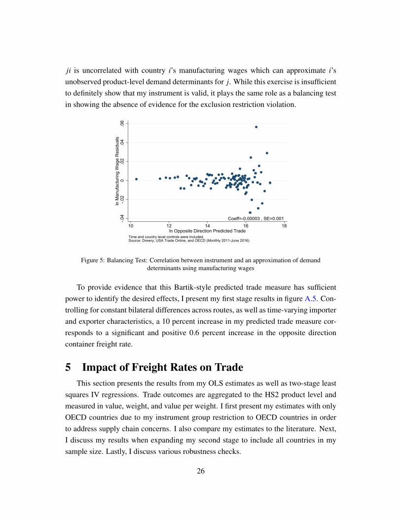
ji is uncorrelated with country i’s manufacturing wages which can approximate i’sunobserved product-level demand determinants for j. While this exercise is insufficientto definitely show that my instrument is valid, it plays the same role as a balancing testin showing the absence of evidence for the exclusion restriction violation.

Coeff=-0.00003 , SE=0.001-.04

-.02

0.0

2.0

4.0

6ln

Man

ufac

turin

g W

age

Res

idua

ls

10 12 14 16 18ln Opposite Direction Predicted Trade

Time and country level controls were included.Source: Drewry, USA Trade Online, and OECD (Monthly 2011-June 2016)

Figure 5: Balancing Test: Correlation between instrument and an approximation of demanddeterminants using manufacturing wages

To provide evidence that this Bartik-style predicted trade measure has sufficientpower to identify the desired effects, I present my first stage results in figure A.5. Con-trolling for constant bilateral differences across routes, as well as time-varying importerand exporter characteristics, a 10 percent increase in my predicted trade measure cor-responds to a significant and positive 0.6 percent increase in the opposite directioncontainer freight rate.

5 Impact of Freight Rates on TradeThis section presents the results from my OLS estimates as well as two-stage least

squares IV regressions. Trade outcomes are aggregated to the HS2 product level andmeasured in value, weight, and value per weight. I first present my estimates with onlyOECD countries due to my instrument group restriction to OECD countries in orderto address supply chain concerns. I also compare my estimates to the literature. Next,I discuss my results when expanding my second stage to include all countries in mysample size. Lastly, I discuss various robustness checks.

26

5.1 Main ResultsPanel A in in table 3 presents the containerized trade value estimates. Column (1)

presents the OLS estimates with separate controls for importer-by-time, exporter-by-time, dyad, and products. A one percent increase in container freight rates is correlatedwith a significant 0.7 percent decrease in trade value. This estimate is robust to con-trolling for comparative advantage with dyad-by-product fixed effects–a one percentincrease in container freight rates corresponds to a significant 0.5 percent decrease intrade value (column (2)). After addressing the potential simultaneity bias with mypredicted return direction trade instrument, the IV estimates are, as expected, morepronounced in magnitude. Column (3) shows that a one percent increase in per unitcontainer freight rates decreases containerized trade value by 3.7 percent with separateproduct and dyad controls. This result is robust to including dyad-by-product controls(column (4))–a one percent increase in freight rates decreases trade value by 2.8 per-cent. The IV approach here yields trade elasticity estimates that are roughly five timesmore sensitive than the OLS estimates.

Panel B in table 3 presents the results using containerized trade weight as the out-come. The weight estimates are overall larger than the value estimates. This is a reflec-tion of trade weight being a closer proxy to quantity while value contains both quantityand price. Prices tend to increase with freight rates while the opposite is true for quan-tity. The OLS estimates in column (1) show that a one percent increase in freight ratescorrespond to a one percent decrease in trade weight. With the inclusion of dyad-by-product controls, the estimate decreases slightly—a one percent increase in freightrates decrease trade weight by 0.8 percent (column (2)). In my IV estimates, a one per-cent increase in container freight rates decreases containerized weight by 4.8 percent(column (3)). With dyad-by-product controls, this estimate decreases slightly—a onepercent increase in container freight rates decreases trade weight by 3.6 percent (col-umn (4)). While the IV estimates here are not directly comparable to the literature, myOLS containerized trade weight estimates are comparable to the volume elasticities forair, truck, and rail (De Palma et al. (2011); Oum, Waters and Yong (1992)).28

Panel C in table 3 presents the containerized value per weight elasticity with re-spect to freight rates results. Containerized value per weight can be calculated usingboth the value and weight variables. This unit value calculation provides a crude mea-

28Their aggregate volume elasticity with respect to transport cost is between -0.8 to -1.6 for air, -0.7to -1.1 for truck, and -0.4 to -1.2 for rail.

27

Table 3: Containerized Trade Demand Estimates for OECD Countries

(1) (2) (3) (4)OLS OLS IV IV

Panel A: ln Trade Valueln Freight Rate -0.676∗∗∗ -0.520∗∗∗ -3.651∗∗∗ -2.795∗∗

(0.148) (0.133) (0.949) (0.903)Panel B: ln Trade Weightln Freight Rate -1.061∗∗∗ -0.837∗∗∗ -4.790∗∗∗ -3.631∗∗∗

(0.196) (0.177) (1.126) (0.969)Panel C: ln Trade Value per Weightln Freight Rate 0.384∗∗∗ 0.317∗∗∗ 1.138∗∗∗ 0.836∗∗∗

(0.0695) (0.0681) (0.224) (0.226)Ex-Time & Im-Time FE Y Y Y YDyad FE Y YProduct FE Y YDyad-Product FE Y YObservations 116887 116887 116887 116887First Stage F 12.38 10.70

Robust standard errors in parentheses are clustered by route. * p < 0.05, ** p < 0.01, *** p < 0.001Results are robust to clustering at the route and product, dyad (two-way route), and dyad with products level. All variables

are in logs. Trade value, weight, and value per weight are aggregated to the HS2 level. Table A.3 presents the first stageregressions. The predicted trade instrument is constructed at the HS4 level with Jan 2003 data using only OECD countries.Second stage is run on OECD countries as well.Fixed Effects explanation: Ex-Time FE is exporter country and time fixed effects; Im-Time FE is importer country and

time fixed effects.Sources: Drewry and USA Trade Online (Monthly 2011-June 2016)

sure of product quality since it is not possible to distinguish whether higher unit valuemeans a higher quality product within the same classification category or across prod-uct categories. The OLS estimate in column (1) shows that a one percent increasein container freight rates increases the product quality in containers by about 0.4 per-cent. When controlling for dyad-by-products, a one percent increase in freight rates in-creases product quality by 0.3 percent (column (2)). In my IV estimates, a one percentincrease in freight rates increases containerized quality by 1.1 percent. This estimatedecreases slightly with dyad-by-product controls—a one percent increase in freightrates increases containerized quality by 0.8 percent. My value per weight IV estimatesare comparable to Hummels and Skiba (2004) who finds a price elasticity with respectto freight cost between 0.8 to 1.41 using two different sets of instruments.

28

5.2 Robustness ChecksMy results are robust to a number of alternative specifications including sample

size expansion, removal of products typically constructed in supply chains, productand time period aggregrations, different product classifications, as well as base yearchange. These results are also robust to alternative levels of clustering—at the routeand product, dyad (two-way route), and dyad with products levels. Overall, the firststage results suggest that my instrument is strong with F-statistics above the standardthreshold of 10 suggested by Staiger and Stock (1994).

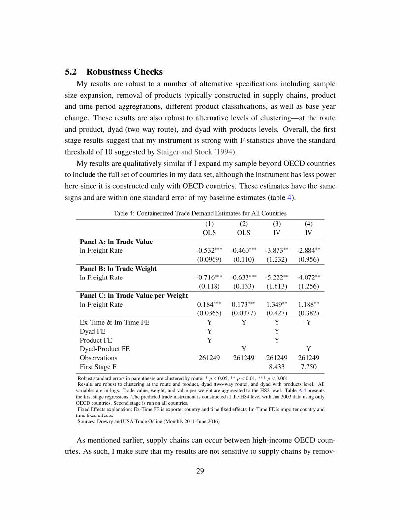
My results are qualitatively similar if I expand my sample beyond OECD countriesto include the full set of countries in my data set, although the instrument has less powerhere since it is constructed only with OECD countries. These estimates have the samesigns and are within one standard error of my baseline estimates (table 4).

Table 4: Containerized Trade Demand Estimates for All Countries

(1) (2) (3) (4)OLS OLS IV IV

Panel A: ln Trade Valueln Freight Rate -0.532∗∗∗ -0.460∗∗∗ -3.873∗∗ -2.884∗∗

(0.0969) (0.110) (1.232) (0.956)Panel B: ln Trade Weightln Freight Rate -0.716∗∗∗ -0.633∗∗∗ -5.222∗∗ -4.072∗∗

(0.118) (0.133) (1.613) (1.256)Panel C: ln Trade Value per Weightln Freight Rate 0.184∗∗∗ 0.173∗∗∗ 1.349∗∗ 1.188∗∗

(0.0365) (0.0377) (0.427) (0.382)Ex-Time & Im-Time FE Y Y Y YDyad FE Y YProduct FE Y YDyad-Product FE Y YObservations 261249 261249 261249 261249First Stage F 8.433 7.750

Robust standard errors in parentheses are clustered by route. * p < 0.05, ** p < 0.01, *** p < 0.001Results are robust to clustering at the route and product, dyad (two-way route), and dyad with products level. All

variables are in logs. Trade value, weight, and value per weight are aggregated to the HS2 level. Table A.4 presentsthe first stage regressions. The predicted trade instrument is constructed at the HS4 level with Jan 2003 data using onlyOECD countries. Second stage is run on all countries.Fixed Effects explanation: Ex-Time FE is exporter country and time fixed effects; Im-Time FE is importer country and

time fixed effects.Sources: Drewry and USA Trade Online (Monthly 2011-June 2016)

As mentioned earlier, supply chains can occur between high-income OECD coun-tries. As such, I make sure that my results are not sensitive to supply chains by remov-

29

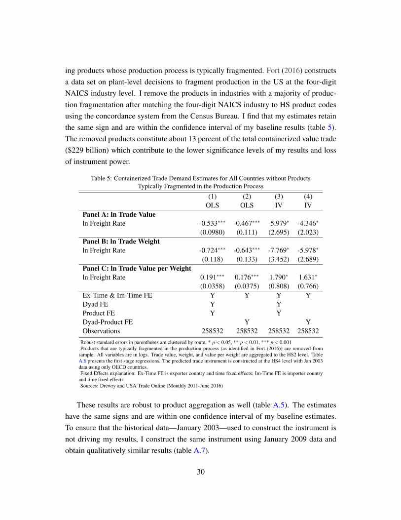
ing products whose production process is typically fragmented. Fort (2016) constructsa data set on plant-level decisions to fragment production in the US at the four-digitNAICS industry level. I remove the products in industries with a majority of produc-tion fragmentation after matching the four-digit NAICS industry to HS product codesusing the concordance system from the Census Bureau. I find that my estimates retainthe same sign and are within the confidence interval of my baseline results (table 5).The removed products constitute about 13 percent of the total containerized value trade($229 billion) which contribute to the lower significance levels of my results and lossof instrument power.

Table 5: Containerized Trade Demand Estimates for All Countries without ProductsTypically Fragmented in the Production Process

(1) (2) (3) (4)OLS OLS IV IV

Panel A: ln Trade Valueln Freight Rate -0.533∗∗∗ -0.467∗∗∗ -5.979∗ -4.346∗

(0.0980) (0.111) (2.695) (2.023)Panel B: ln Trade Weightln Freight Rate -0.724∗∗∗ -0.643∗∗∗ -7.769∗ -5.978∗

(0.118) (0.133) (3.452) (2.689)Panel C: ln Trade Value per Weightln Freight Rate 0.191∗∗∗ 0.176∗∗∗ 1.790∗ 1.631∗

(0.0358) (0.0375) (0.808) (0.766)Ex-Time & Im-Time FE Y Y Y YDyad FE Y YProduct FE Y YDyad-Product FE Y YObservations 258532 258532 258532 258532

Robust standard errors in parentheses are clustered by route. * p < 0.05, ** p < 0.01, *** p < 0.001Products that are typically fragmented in the production process (as identified in Fort (2016)) are removed from

sample. All variables are in logs. Trade value, weight, and value per weight are aggregated to the HS2 level. TableA.6 presents the first stage regressions. The predicted trade instrument is constructed at the HS4 level with Jan 2003data using only OECD countries.Fixed Effects explanation: Ex-Time FE is exporter country and time fixed effects; Im-Time FE is importer country

and time fixed effects.Sources: Drewry and USA Trade Online (Monthly 2011-June 2016)

These results are robust to product aggregation as well (table A.5). The estimateshave the same signs and are within one confidence interval of my baseline estimates.To ensure that the historical data—January 2003—used to construct the instrument isnot driving my results, I construct the same instrument using January 2009 data andobtain qualitatively similar results (table A.7).

30

Since my data is at the monthly period, these elasticities should be higher than amore aggregated time period since they take into account the willingness of importersand exporters to substitute shipping their goods across time. Their ability to substituteis easier over a shorter time period compared to a longer period. I show that this is thecase—aggregating the monthly estimation to the annual level reduces the elasticity byat least half or more (table A.9). Steinwender (Forthcoming) finds the same reductionin her elasticities when aggregating her daily data upwards.

Last but not least, I evaluate these estimates using the Rauch (1999) test which pre-dicts that these elasticities should be more elastic for more homogeneous goods. Usingthe concorded product classifications from Rauch (1999), I divide my sample into ho-mogeneous goods (grouping both homogeneous and reference-price goods from hisclassification) and differentiated goods. I show that the differentiated goods samplehave much smaller elasticities in magnitude compared to more homogeneous goodsacross all three outcome variables (table A.11). Shapiro (2015) finds the same magni-tude differences in his elasticities after dividing his sample into these product classifi-cations.

6 CounterfactualUtilizing the trade elasticities from my IV results along with the trade and transport

model, I analyze a doubling of US import tariff on its OECD partners from the 2014average of 1.16 percent. Comparing the simulated trade prediction from my modelto predictions from a model with exogenous transport costs allows me to quantify theimportance of the round trip effect. I first describe the calibration process and thenmove on to estimation as well as my counterfactual results.

6.1 Taking the Model to DataTariff rates are taken from the trade-weighted effectively applied tariff rates for

manufactures from the World Bank’s World Integrated Trade Solution (WITS) database.Input prices are approximated by hourly manufacturing wages from the OECD follow-ing Eaton and Kortum (2002). The use of OECD wages limits the countries in thisanalysis. Specifically, the lack of comparable manufacturing wages excludes manyAsian countries like China and Hong Kong. The round trip marginal cost for each portpair is the sum of the freight rates going both ways (equation (6)).

The price elasticity of demand, σ , is calculated using the trade value demand elas-

31

ticity from my empirical results. The elasticity of trade value with respect to transportcost predicted by the theory model (equation (7)) is:

∂Xi jt

∂Ti jt

Ti jt

Xi jt= (1−σ)

Ti j

wiτi j +Ti j≡ α (16)

This elasticity is equivalent to the estimated demand elasticity in my empirical section,α . In order to obtain σ , I approximate the freight rate share of price ( Ti j

wiτi j+Ti j) with the

estimate by Irarrazabal, Moxnes and Opromolla (2015). They calculate that per unittrade cost is about 14 percent of the median price.29 The price elasticity of demandcalculated from equation (16) is 21.7.

This price elasticity of demand estimate, taking into account the endogeneity oftransport cost and trade, implies a four- to five-fold increase in my estimates whentransport costs are assumed to be exogenous (table 3). This increase is in line withBaier and Bergstrand (2007) who finds a similar five-fold increase in the effect of freetrade agreements (FTAs) on trade flows after taking into account of the endogeneity ofFTAs. Trefler (1993) estimates a larger ten-fold increase in the impact of nontariff tradebarriers (NTBs) when trade protection is modeled endogenously compared to when itis treated as exogenous. Furthermore, both my weight and quality elasticities are inthe ballpark of other studies (Clark et al. (2005), Oum, Waters and Yong (1992) aswell as Hummels and Skiba (2004)). This gives me confidence that my value elasticityestimate, while larger than typically seen in the literature, is not unreasonable. Myresults are also robust to a number of alternative specifications.30

That being said, there are a few reasons that this estimate could be large. First, therecould be potential substitution across months. My data is at the monthly or bimonthlylevel. If the freight rates for one month increases, an importer could wait until the nextmonth to import their goods. The literature typically estimates these elasticities at theannual level which makes these types of substitution less applicable. In fact, I find thatmy elasticities decline by at least half when aggregating my estimation to the annuallevel (table A.9). Steinwender (Forthcoming) finds the same decline in her elasticitieswhen aggregating her daily data as well. Second, there could be potential substitutionacross US ports (LA/LB, NY, and Houston). If the freight rates out of the Houston port

29It is acknowledged here that per unit trade cost does not just include transport cost but also quotasand per unit tariffs. However, the significance of transport costs has been increasing in recent years dueto global decreases in tariffs and other formal trade barriers (Hummels (2007)). As such, I assume herethat transport cost make up most of the per unit trade cost.

30See the robustness checks in the results section for more details.

32

increases, an exporter could choose to export out of the New York port. Typically theseelasticities are estimated at the country level and these types of substitution would notapply.

The remaining preference parameter and the loading factor are chosen to match theobserved trade value and freight rates in my data set given the equilibrium conditionsbelow for each country pair. The preference parameter ai j captures j’s preference fori’s good. The loading factor li j captures the average container volume required perquantity of good traded along route i j. This relaxes the balanced trade quantity as-sumption in the theory model since both the preference and loading parameters willadjust in order to balance the equilibrium quantity of container volumes between i andj, which is the loading factor multiplied by the quantity of goods. The loading factoraffects the traded goods price (equation (2)) as well as the profits of the transport firms(equation (5)):

pi j = w jτi j +Ti j/li j

πi, j = Ti jli jQi j +Tjil jiQ ji− c←→i j max{li jQi j, l jiQ ji}where Qi j is the quantity of goods traded on route i j. In equilibrium, the containervolumes between i and j are the same: li jQ∗i j = l jiQ∗ji.

The equilibrium freight rates and containerized trade value for route i j, includingloading factors li j and l ji, can be derived from the price and profit functions above aswell as the optimality conditions from the theory section (equations (6) and (7)):

T ∗i j =l ji

Yi j +1w jτ ji +

c←→i j

1+Yi j− 1

li j

11+Y−1

jiwiτi j

X∗i j = pi jQi j =

[σ

σ −11

ai j

]−σ [ 11+Yi j

(wiτi j +

l ji

li j

(w jτ ji + c←→i j

))]1−σ

where Yi j =a ji

ai j

(l ji

li j

)1+1/σ

(17)

6.2 Counterfactual: Doubling US import tariffsSince my model is just identified, I am able to match the observed freight rates

and trade value data exactly. The results below are based on 2014 data. Using myestimated parameters, I construct an out of sample fit for the next year, 2015. I find apositive correlation of 0.6 for trade value and 0.7 for freight rates (figure A.7).

Table 6 shows that trade predictions after doubling US import tariffs on its OECDtrading partners from a trade-weighted average of 1.16 percent in 2014. The first two

33

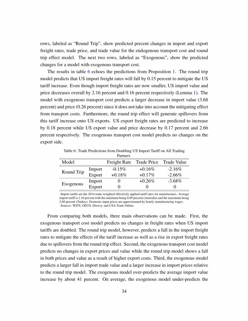
rows, labeled as “Round Trip”, show predicted percent changes in import and exportfreight rates, trade price, and trade value for the endogenous transport cost and roundtrip effect model. The next two rows, labeled as “Exogenous”, show the predictedchanges for a model with exogenous transport cost.

The results in table 6 echoes the predictions from Proposition 1. The round tripmodel predicts that US import freight rates will fall by 0.15 percent to mitigate the UStariff increase. Even though import freight rates are now smaller, US import value andprice decreases overall by 2.16 percent and 0.16 percent respectively (Lemma 1). Themodel with exogenous transport cost predicts a larger decrease in import value (3.68percent) and price (0.26 percent) since it does not take into account the mitigating effectfrom transport costs. Furthermore, the round trip effect will generate spillovers fromthis tariff increase onto US exports. US export freight rates are predicted to increaseby 0.18 percent while US export value and price decrease by 0.17 percent and 2.66percent respectively. The exogenous transport cost model predicts no changes on theexport side.

Table 6: Trade Predictions from Doubling US Import Tariff on All TradingPartners

Model Freight Rate Trade Price Trade Value

Round TripImport -0.15% +0.16% -2.16%Export +0.18% +0.17% -2.66%

ExogenousImport 0 +0.26% -3.68%Export 0 0 0

Import tariffs are the 2014 trade-weighted effectively applied tariff rates for manufactures. Averageimport tariff is 1.16 percent with the minimum being 0.09 percent (Australia) and the maximum being2.68 percent (Turkey). Domestic input prices are approximated by hourly manufacturing wages.Sources: WITS, OECD, Drewry, and USA Trade Online.

From comparing both models, three main observations can be made. First, theexogenous transport cost model predicts no changes in freight rates when US importtariffs are doubled. The round trip model, however, predicts a fall in the import freightrates to mitigate the effects of the tariff increase as well as a rise in export freight ratesdue to spillovers from the round trip effect. Second, the exogenous transport cost modelpredicts no changes in export prices and value while the round trip model shows a fallin both prices and value as a result of higher export costs. Third, the exogenous modelpredicts a larger fall in import trade value and a larger increase in import prices relativeto the round trip model. The exogenous model over-predicts the average import valueincrease by about 41 percent. On average, the exogenous model under-predicts the

34

average import and export changes by 25 percent. These over- and under-predictionestimates are robust to other trade elasticity estimates as well. Using a trade elasticityof 5, the elasticity suggested by Head and Mayer (2014), the exogenous model stillover-predicts the average import value increase by about 40 percent and under-predictstotal trade changes by about 18 percent.

These differences in trade predictions have important policy implications. If a coun-try chooses to pursue protectionist policies by increasing their import tariffs, a trademodel with exogenous transport cost will first over-predict the level of protection theyare affording their local industries—the fall in imports from their trading partners—with no other impact on exports and transport costs. As a result, the exogenous modelwill predict an increase in the trade balance gap between the country’s exports andimports with all its partners by about 4 percent. However, a model which takes into ac-count endogenous transport costs and the round trip effect will paint a different picture:while the country’s imports fall so will its exports. The country will over-predict itsincreased level of protection by about 41 percent in value and its overall trade balancewill decrease instead by about 0.5 percent.

In order to calculate a tariff equivalent of the round trip effect, I calculate the changein export prices due to increases in US import tariffs. From the proof for Lemma 1 andequation (25) in the Theory Appendix, the derivative of US export prices with respectto US import tariffs is a positive constant. As such, the round trip effect from thismodel predicts a constant export tax of 0.2 percent on prices when US import tariffs onits partners are increased by a factor of one.

The results from this counterfactual are calculated across 22 port-level routes be-tween the US and its OECD trading partners. Figure 6 shows that this increase inexport prices are different across routes, ranging from a 0.01 percent increase for theMelbourne-LA route which has a very low initial US tariff of 0.9 percent to a 0.68percent increase for the Istanbul-Houston route which has a higher initial tariff of 2.7percent. Since the counterfactual exercise here increases initial US tariffs by a factor ofone, countries with higher US initial tariffs will see a bigger increases in export prices.Conditional upon the port pairs being in the same countries, the differences in exportprices are driven by route-specific data and parameters. For example, the Genoa-NewYork and Genoa-Houston routes have different changes in export prices although theUS import tariff for Italy is the same for both routes. US exports on the Genoa-NewYork route is about 3.5 times more in value compared to US imports, resulting in a

35

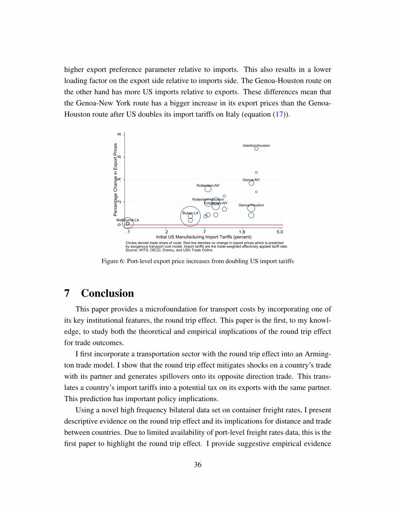
higher export preference parameter relative to imports. This also results in a lowerloading factor on the export side relative to imports side. The Genoa-Houston route onthe other hand has more US imports relative to exports. These differences mean thatthe Genoa-New York route has a bigger increase in its export prices than the Genoa-Houston route after US doubles its import tariffs on Italy (equation (17)).

Busan-LA

Melbourne-LA

Rotterdam-NY

Rotterdam-Houston

Istanbul-Houston

Felixstowe-NY

Genoa-NY

Genoa-Houston

0.2

.4.6

.8Pe

rcen

tage

Cha

nge

in E

xpor

t Pric

es

.1 .2 .7 1.8 5.0Initial US Manufacturing Import Tariffs (percent)

Circles denote trade share of route. Red line denotes no change in export prices which is predictedby exogenous transport cost model. Import tariffs are the trade-weighted effectively applied tariff rates.Source: WITS, OECD, Drewry, and USA Trade Online.

Figure 6: Port-level export price increases from doubling US import tariffs

7 ConclusionThis paper provides a microfoundation for transport costs by incorporating one of

its key institutional features, the round trip effect. This paper is the first, to my knowl-edge, to study both the theoretical and empirical implications of the round trip effectfor trade outcomes.

I first incorporate a transportation sector with the round trip effect into an Arming-ton trade model. I show that the round trip effect mitigates shocks on a country’s tradewith its partner and generates spillovers onto its opposite direction trade. This trans-lates a country’s import tariffs into a potential tax on its exports with the same partner.This prediction has important policy implications.

Using a novel high frequency bilateral data set on container freight rates, I presentdescriptive evidence on the round trip effect and its implications for distance and tradebetween countries. Due to limited availability of port-level freight rates data, this is thefirst paper to highlight the round trip effect. I provide suggestive empirical evidence

36

for two main predictions from my theory model: (1) that freight rates are negativelycorrelated within port pairs, and (2) a country’s imports from its partner are positivelycorrelated with its export transport cost to the same partner. The same applies for acountry’s exports and its import transport cost. Both these correlations indicate thepresence of the round trip effect.

I develop an identification strategy utilizing the round trip effect to estimate thecontainerized trade elasticity with respect to freight rates. I find that a one percentincrease in average freight rates will decrease average containerized trade value by2.8 percent, decrease average containerized trade weight by 3.6 percent, and increaseaverage containerized trade quality by 0.8 percent.

In order to estimate the magnitude of the potential export tax from protectionistpolicies like import tariffs, I estimate my trade and transportation model using mytrade elasticity and simulate a counterfactual where the US doubles its import tariffs onall of its partners from an average of 1.2 percent. I show that this tariff increase willnot just decrease US imports but also US exports to these partners. A trade model withexogenous transport costs would over-predict the import decrease by 41 percent, notpredict any associated bilateral export decrease at all, and under-predict the total tradechanges by 25 percent. Overall, this model predicts an export tax of about 0.2 percenton prices when US import tariffs are doubled.

Future work includes relaxing the perfect competition assumption in the future tostudy the effects of market power in transportation in the presence of the round tripeffect. Concentration in the containership industry has increase over the years throughcapacity-sharing alliances. However, since there are economies of scale to transporta-tion, these alliances have potential efficiency gains from increased capacity utilizationon each ship. Given these factors, it would be worth examining if containership com-panies should be allowed to form further alliances.

ReferencesAlchian, Armen Albert, and William Richard Allen. 1964. University Economics. Belmont,

CA: Wadsworth Publishing Company.Anderson, James E, and Eric Van Wincoop. 2004. “Trade costs.” Journal of Economic liter-

ature, 42(3): 691–751.Asturias, Jose, and Scott Petty. 2013. “Endogenous Transportation Costs.” University of Min-

nesota.

37

Autor, David H., David Dorn, and Gordon H. Hanson. 2013. “The China syndrome: Locallabor market effects of import competition in the United States.” American Economic Review,103(6): 2121–68.

Autor, David H., David Dorn, Gordon H. Hanson, and Jae Song. 2014. “Trade Adjustment:Worker Level Evidence*.” The Quarterly Journal of Economics.

Baier, Scott L, and Jeffrey H Bergstrand. 2007. “Do free trade agreements actually increasemembers’ international trade?” Journal of international Economics, 71(1): 72–95.

Bartik, Timothy J. 1991. Who Benefits from State and Local Economic Development Policies?Books from Upjohn Press, W.E. Upjohn Institute for Employment Research.

Behrens, Kristian, and Pierre M Picard. 2011. “Transportation, freight rates, and economicgeography.” Journal of International Economics, 85(2): 280–291.

Bernhofen, Daniel M, Zouheir El-Sahli, and Richard Kneller. 2016. “Estimating the effectsof the container revolution on world trade.” Journal of International Economics, 98: 36–50.

Brancaccio, Giulia, Myrto Kalouptsidi, and Theodore Papageorgiou. 2017. “Geography,Search Frictions and Endogenous Trade Costs.” National Bureau of Economic Research.

Chaney, Thomas. 2008. “Distorted gravity: the intensive and extensive margins of interna-tional trade.” The American Economic Review, 98(4): 1707–1721.

Chang, Yu-Chia, Ruo-Shan Tseng, Guan-Yu Chen, Peter C Chu, and Yung-Ting Shen.2013. “Ship routing utilizing strong ocean currents.” Journal of Navigation, 66(06): 825–835.

Clark, Chris, Helen Tammela Naughton, Bruce Proulx, and Paul Thoma. 2005. “A sur-vey of the freight transportation demand literature and a comparison of elasticity estimates.”Institute for Water Resources US Army Corps of Engineers Alexandria, Virginia.

Cosar, A. Kerem, and Banu Demir Pakel. 2017. “Shipping inside the Box: Containerizationand Trade.”

Costinot, Arnaud, and Ivan Werning. 2017. “The Lerner Symmetry Theorem: Generaliza-tions and Qualifications.”

Demirel, Erhan, Jos Van Ommeren, and Piet Rietveld. 2010. “A matching model for thebackhaul problem.” Transportation Research Part B: Methodological, 44(4): 549–561.

De Palma, Andre, Robin Lindsey, Emile Quinet, and Roger Vickerman. 2011. A handbookof transport economics. Edward Elgar Publishing.

Donaldson, Dave. Forthcoming. “Railroads of the Raj: Estimating the impact of transportationinfrastructure..” American Economic Review.

Ducruet, Cesar, and Theo Notteboom. 2012. “Developing liner service networks in containershipping.” Maritime Logistics: A complete guide to effective shipping and port management,77–100.

38

Eaton, Jonathan, and Samuel Kortum. 2002. “Technology, geography, and trade.” Econo-metrica, 70(5): 1741–1779.

Fort, Teresa C. 2016. “Technology and Production Fragmentation: Domestic versus ForeignSourcing.” National Bureau of Economic Research Working Paper 22550.

Francois, Joseph F, and Ian Wooton. 2001. “Trade in international transport services: the roleof competition.” Review of International Economics, 9(2): 249–261.

Friedt, Felix L. 2017. “Trade Policy Outcomes in the Presence of Asymmetric Transport Costs:Theory and Evidence.” University of Oregon.

Friedt, Felix Laurence, and Wesley W Wilson. 2015. “Trade, Transportation and TradeImbalances: An Empirical Examination of International Markets and Backhauls.” SSRN2636983.

Fugazza, Marco, and Jan Hoffmann. 2016. “Bilateral Liner Shipping Connectivity since2006..” Policy Issues in International Trade and Commodities, Study Series, , (72).

Hammer, Alexander B. 2006. The Dynamic Structure of US-China Trade, 1995-2004. UnitedStates International Trade Commission.

Head, Keith, and Thierry Mayer. 2014. “Gravity Equations: Workhorse, Toolkit, and Cook-book.” Handbook of International Economics, 4: 131.

Hummels, David. 2007. “Transportation costs and international trade in the second era of glob-alization.” The Journal of Economic Perspectives, 21(3): 131–154.

Hummels, David, and Alexandre Skiba. 2004. “Shipping the good apples out? An empiricalconfirmation of the Alchian-Allen conjecture.” Journal of Political Economy, 112(6): 1384–1402.

Hummels, David, Volodymyr Lugovskyy, and Alexandre Skiba. 2009. “The trade reduc-ing effects of market power in international shipping.” Journal of Development Economics,89(1): 84–97.

Irarrazabal, Alfonso, Andreas Moxnes, and Luca David Opromolla. 2015. “The tip of theiceberg: a quantitative framework for estimating trade costs.” Review of Economics andStatistics, 97(4): 777–792.

Ishikawa, Jota, and Nori Tarui. 2016. “Backfiring with Backhaul Problems: Trade and indus-trial policies with endogenous transport costs.”

Jonkeren, Olaf, Erhan Demirel, Jos van Ommeren, and Piet Rietveld. 2011. “Endogenoustransport prices and trade imbalances.” Journal of Economic Geography, 11(3): 509–527.

Korinek, Jane. 2008. “Clarifying trade costs in maritime transport.” Organization for Eco-nomic Co-operation and Development TAD/TC/WP (2008), 10.

Lerner, Abba P. 1936. “The symmetry between import and export taxes.” Economica,3(11): 306–313.

39

Limao, Nuno, and Anthony J Venables. 2001. “Infrastructure, geographical disadvantage,transport costs, and trade.” The World Bank Economic Review, 15(3): 451–479.

Melitz, Marc J. 2003. “The Impact of Trade on Intra-Industry Reallocations and AggregateIndustry Productivity.” Econometrica, 71(6): 1695–1725.

Miao, Jianjun. 2006. “A search model of centralized and decentralized trade.” Review of Eco-nomic Dynamics, 9(1): 68–92.

Mostashari, Shalah. 2010. “Vertical specialization, intermediate tariffs, and the pattern oftrade: assessing the role of tariff liberalization to US bilateral trade 1989-2001.” UT Austin.

Oum, Tae Hoon, William G Waters, and Jong-Say Yong. 1992. “Concepts of price elastici-ties of transport demand and recent empirical estimates: an interpretative survey.” Journal ofTransport Economics and policy, 139–154.

Pigou, AC, and FW Taussig. 1913. “Railway rates and joint costs.” The Quarterly Journal ofEconomics, 27(4): 687–694.

Rauch, James E. 1999. “Networks versus markets in international trade.” Journal of interna-tional Economics, 48(1): 7–35.

Rodrigue, Jean-Paul, Claude Comtois, and Brian Slack. 2013. The geography of transportsystems. Routledge.

Rua, Gisela. 2014. “Diffusion of containerization.” Finance and Economics Discussion SeriesStaff working paper 201488. Federal Reserve Board, Washington, DC.

Samuelson, Paul A. 1954. “The transfer problem and transport costs, II: Analysis of effects oftrade impediments.” The Economic Journal, 64(254): 264–289.

Shapiro, Joseph S. 2015. “Trade Costs, CO2, and the Environment.” American Economic Jour-nal: Economic Policy.

Staiger, Douglas O, and James H Stock. 1994. “Instrumental variables regression with weakinstruments.”

Steinwender, Claudia. Forthcoming. “The Real Effects of Information Frictions:” When theStates and the Kingdom became United”.” American Economic Review.

Tanaka, Kiyoyasu, and Kenmei Tsubota. 2016. “Directional imbalance in freight rates: evi-dence from Japanese inter-prefectural data.” Journal of Economic Geography, lbw005.

Trefler, Daniel. 1993. “Trade liberalization and the theory of endogenous protection: an econo-metric study of US import policy.” Journal of political Economy, 138–160.

Wong, Woan Foong. 2018. “The Round Trip Effect: Endogenous Transport Costs and Interna-tional Trade.” University of Oregon.

40

A Appendix

A.1 Simple Model of the Round Trip EffectThere are two transport markets, one going from origin j to destination i (route ji)

and the other going back from i to j (route i j). I present both these markets without theround trip effect and then introduce the round trip effect and its implications.

I assume linear transport demand functions for both routes ji and i j:

QDji = Di−diTji and QD

i j = D j−d jTi j (18)

where QDji is the transport quantity demanded on route ji and Tji is the transport cost,

or transport price, on the same route. Di is country i’s demand intercept parameterfor transport services from j (Di > 0) while di is its demand slope parameter (di > 0).Similar notation applies for the opposite direction variables on route i j.

A.1.1 Model absent the round trip effectFollowing the demand assumption, I also assume linear transport supply. Absent

the round trip effect, transport supply for both routes are separately determined:

QSji =C ji + c jiTji and QS

i j =Ci j + ci jTi j (19)

where QSji is the transport quantity supplied on route ji and Tji is the transport cost

or price on the same route. Route ji’s fixed cost of transport supply is C ji ≥ 0 (forexample, the cost of hiring a captain) and its marginal cost is c ji > 0 (for example, fuelcost). This positive marginal cost generates an upward sloping supply curve.31

The equilibrium transport price and quantity for route ji and i j are:

T ∗ji =1

di + c ji

(Di−C ji

)and Q∗ji =

1di + c ji

(c jiDi +diC ji

)T ∗i j =

1d j + ci j

(D j−Ci j

)and Q∗i j =

1d j + ci j

(ci jD j +d jCi j

) (20)

where any demand and supply parameter changes on a route only affects the transportprice and quantity of that route—a positive demand shock on route ji (Di increase) willonly affect the route ji transport price and quantity. Both these markets are illustratedin Panel A of figure A.2. The top graph is the transport market for route ji while thebottom graph is the transport market for return direction route i j.

31One interpretation is that there are a continuum of small transport firms providing transport betweenthe two countries who face heterogenous marginal costs.

41

A.1.2 Model with the round trip effectIn the presence of the round trip effect, transport supply for both routes are jointly

determined. For simplicity, I assume that the demand for transport between these twomarkets are symmetric enough that transport firms will always be at full capacity goingbetween them.32 As such, the supply of transport on both routes (

←→i j ) will be the same.

The combined transport supply for both routes includes the fixed cost of transport (C←→i j )and the marginal cost of transport (c←→i j ):

33

QSi j = QS

ji ≡ QS←→i j=C←→i j + c←→i j

(Tji +Ti j

)(21)

The equilibrium transport prices and quantity for routes i j and ji with the roundtrip effect are now no longer independently determined:

T ∗ji =1

c←→i j di + c←→i j d

j +did j

[(d j + c←→i j

)Di− c←→i j D

j−d jC←→i j

]T ∗i j =

1c←→i j d

i + c←→i j dj +did j

[(di + c←→i j

)D j− c←→i j D

i−diC←→i j

]Q∗ji = Q∗i j ≡ Q∗ =

C←→i j

c←→i j di + c←→i j d

j +did j +Di(

d j + c←→i j

)di

+D j(

di + c←→i j

)d j

(22)

where the equilibrium transport price on route ji (T ∗ji) is increasing in destination coun-try i’s demand intercept for j (Di) but decreasing in the fixed cost of round trip transport(C←→i j ). Additionally, it is now a function of the origin country i’s demand parameters:it is decreasing in the origin country j’s demand intercept for i’s good (D j). This latterprediction is due to the round trip effect. The same applies for the transport price onroute i j (T ∗ji). The equilibrium quantity of transport services for both routes is increas-ing in the demand intercepts in both countries (Di and D j) and the round trip fixed costof transport (C←→i j ) but decreasing in both countries’ demand slopes and the round tripmarginal cost (c←→i j ).

Both the transport markets for routes ji and i j are illustrated in Panel B of figureA.2. In the presence of the round trip effect, both these markets are now linked viatransport supply and the equilibrium transport quantity is the same.

Now suppose there is a positive demand shock on route ji where i’s demand for j’s

32If demand between these markets are asymmetric enough, there may be some transport firms goingempty one way (Ishikawa and Tarui (2016)). Potential modeling modifications can and have been madein order to accommodate this feature, for example a search framework. The theory section and onlineappendix B elaborates.

33These costs are assumed to be the same here. It is possible to relax this assumption without changingthe main results.

42

good(Di) increases while holding the other parameters constant. This raises the equi-librium transport price on route ji (equation (22)) as well as the equilibrium transportquantity.Through the round trip effect, the equilibrium quantity on opposite route i jalso increases. Since the demand on opposite route i j has not changed, this increasedtransport quantity decreases its transport price (equation (22)). As such, in the pres-ence of the round trip effect, a positive demand shock on route ji does not just increasethe equilibrium transport price and quantity on that route, it also decreases the equi-librium transport price on the opposite route i j. The blue lines in Panel B of figureA.2 illustrates this demand shock graphically where Q′Dji is the new demand curve afterthe shock on i’s demand intercept for j (Di > Di). Q′Si j is the new transport supply onopposite route i j which results in a lower equilibrium transport price T ′∗i j .34

A.2 Theory Appendix

Endogenous Transport Cost & Round Trip Effect Model: Symmetric EquilibriumIn the special case where countries i and j are symmetric, the preference parameters

in both countries would be the same: ai j = a ji ≡ a. As such, the freight rates each waybetween i and j will be the same–one half of the round trip marginal cost: T Sym

i j =

T Symji = 1

2c←→i j . The symmetric equilibrium prices, quantities, and values are a functionof the domestic wages and tariffs in both countries as well as the round trip marginalcost:

pSymi j = pSym

ji =12

(w jτ ji +wiτi j + c←→i j

)qSym

i j = qSymji =

[σ

σ −11a

12

(w jτ ji +wiτi j + c←→i j

)]−σ

XSymi j = XSym

ji =

[σ

σ −11a

]−σ [12

(w jτ ji +wiτi j + c←→i j

)]1−σ

(23)

Endogenous Transport Cost & Round Trip Effect Model: Opposite DirectionEquilibrium

The equilibrium freight rate for route ji is

T Rji =

11+A ji

(wiτi j + c←→i j

)− 1

1+A−1ji

(w jτ ji

), A ji =

ai j

a ji(24)

34The new lower opposite route transport price T ′∗i j will also shift the route ji supply (Q′Sji , equation(21)).

43

The equilibrium trade price, quantity, and value of country j’s good in i is

pRji =

11+A ji

(wiτi j +w jτ ji + c←→i j

)qR

ji =

[σ

σ −11

a ji

11+A ji

(wiτi j +w jτ ji + c←→i j

)]−σ

XRji =

[σ

σ −11

a ji

]−σ [ 11+A ji

(wiτi j +w jτ ji + c←→i j

)]1−σ

where A ji =ai j

a ji

(25)

Proof of Lemma 1 This lemma can be proven via direct calculation. In the exoge-nous transport cost model, the derivative of j’s import price from i with respect to its

import tariff on i is positive (equation (3)):∂ pExo

i j∂τi j

= wi > 0. From equation (4), thederivative of j’s import quantity from i with respect to its import tariff on i is nega-

tive:∂qExo

i j∂τi j

= −σwi(wiτi j + ci j

)−σ−1[

σ

σ−11

ai j

]−σ

< 0. From equation (4), the deriva-tive of j’s import quantity from i with respect to its import tariff on i is also negative:∂XExo

i j∂τi j

=−(σ −1)wi(wiτi j + ci j

)−σ[

σ

σ−11

ai j

]−σ

< 0.In the endogenous transport cost model with the round trip effect, an increase in

j’s import tariff on i decreases j’s import transport cost from i. The derivative of thetransport cost from i to j with respect to j’s import tariff on i is negative (equation (9)):∂T R

i j∂τi j

=− 11+Ai j

wi < 0.The increase in j’s import tariff on i will also decrease the price of j’s imports from

i through its import transport cost decrease. The derivative of the price of country i’sgood in country j with respect to j’s import tariff on i is positive (equation (10)) andthe same magnitude as the the derivative of the transport cost from i to j with respect

to j’s import tariff on i:∂ pR

i j∂τi j

= 11+Ai j

wi > 0.Country j’s equilibrium import quantity from i will decrease with the increase of

j’s import tariff on i, as does its equilibrium trade value from i. From equation (11), thederivative of the trade quantity from i to j with respect to j’s import tariff on i is neg-

ative:∂qR

i j∂τi j

= −σwi

(σ

σ−11

ai j( 1

1+Ai j

)−σ (w jτ ji +wiτi j + c←→i j

)−σ−1< 0. From equation

(11), the derivative of the trade value from i to j with respect to j’s import tariff on i is

negative:∂XR

i j∂τi j

=−(σ −1)wi

(1

1+Ai j

)1−σ [σ

σ−11

ai j

(w jτ ji +wiτi j + c←→i j

)]−σ

< 0.The mitigating effects from the endogenous transport cost and round trip effect

model is clear when comparing the import trade changes between the two models. The

44

import quantity fall due to tariffs for the exogenous transport cost model is larger:

∂qExoi j /∂τi j

∂qRi j/∂τi j

=

(wiτi j + ci j

)−σ−1

11+Ai j

(wiτi j +w jτ ji + c←→i j

)−σ−1 > 0

The same can be shown for the import value fall between the models:∂XExo

i j /∂τi j

∂XRi j/∂τi j

=

(wiτi j + ci j

)−σ(1

1+Ai j

)1−σ (wiτi j +w jτ ji + c←→i j

)−σ> 0

Due to the round trip effect, an increase in j’s import tariff on i also affects j’sexports to i. First, j’s export transport cost to i increases in order to compensate for thefall in inbound transport demand from i to j. The derivative of the transport cost from j

to i with respect to j’s import tariff on i is positive (equation (24)):∂T R

ji∂τi j

= 11+A−1

i jwi > 0.

Unlike the comparative statics involving j’s preference of i’s goods, the amount ofdecrease in j’s import transport cost from i is no longer the same as the amount ofincrease in j’s export transport cost to i.

The increase in j’s import tariff on i also increases j’s export price to i. The deriva-tive of j’s export price to i with respect to j’s import tariff on i is positive (equation

(25)):∂ pR

ji∂τi j

= 11+A−1

i jwi > 0. This export price increase is the same amount as j’s import

transport cost increase.Lastly, the increase in j’s import tariff on i decreases j’s export quantity and value to

i. The derivative of j’s export quantity to i with respect to j’s import tariff on i is nega-

tive (equation (25)):∂qR

ji∂τi j

=−σwi

(σ

σ−11

a ji( 1

1+A−1i j

)−σ (w jτ ji +wiτi j + c←→i j

)−σ−1< 0.

The derivative of j’s export value to i with respect to j’s preference for i’s good is nega-

tive (equation (25)):∂XR

ji∂τi j

=−(σ −1)wi

(1

1+A−1i j

)1−σ [σ

σ−11

a ji

(w jτ ji +wiτi j + c←→i j

)]−σ

<

0.

Proof of Lemma 2 This lemma can be proven via direct calculation. In the exogenoustransport cost model, the derivative of j’s import quantity from i with respect to j’s pref-

erence for i’s good is positive (equation (4)):∂qExo

i j∂ai j

= σaσ−1i j

[σ

σ−1

(wiτi j + ci j

)]−σ> 0.

The derivative of j’s import value from i with respect to j’s preference for i’s good is

also positive (equation (4)):∂XExo

i j∂ai j

= σaσ−1i j

(σ

σ−1

)−σ (wiτi j + ci j)1−σ

> 0. Countryj’s import price from i does not change with its preference for i’s good (equation (3)):

45

∂ pExoi j

∂ai j= 0.

In the endogenous transport cost and round trip effect model, I first establish thatthe derivative of the loading factor and preference ratio from i to j with respect to j’spreference for i’s good is negative, ∂Ai j

∂ai j= − 1

ai jAi j < 0. The derivative of the loading

factor and preference ratio from j to i with respect to j’s preference for i’s good ispositive, ∂A ji

∂ai j= 1

ai jA−1

i j > 0.An increase in j’s preference for i’s good increases j’s import transport cost from

i. The derivative of the transport cost from i to j with respect to j’s preference for i’s

good is positive (equation (9)):∂T R

i j∂ai j

= 1ai j

11+Ai j

11+A−1

i j

[wiτi j +w jτ ji + c←→i j

]> 0.

The increase in j’s preference for i’s good will also increase the price of j’s importsfrom i through the increase in j’s import transport cost from i. The derivative of theprice of country i’s good in country j with respect to j’s preference for i’s good is pos-itive (equation (10)) and the same as the the derivative of the transport cost from i to j

with respect to j’s preference for i’s good:∂ pR

i j∂ai j

= 1ai j

11+Ai j

11+A−1

i j

[wiτi j +w jτ ji + c←→i j

]>

0.Even though the increase in j’s preference for i raises the price of its imports from i,

j’s equilibrium import quantity from i still increases as does its equilibrium trade valuefrom i. From equation (11), the derivative of the trade quantity from i to j with respectto j’s preference for i’s good is positive: ∂qR

i j∂ai j

=σ

(1

ai j

)1−σ (1

1+Ai j

)1−σ [σ

σ−1

(w jτ ji +wiτi j + c←→i j

)]−σ

>

0. From equation (11), the derivative of the trade value from i to j with respect to j’spreference for i’s good is positive: ∂XR

i j∂ai j

=(σ +Ai j)(

1ai j

)1−σ (1

1+Ai j

)2−σ [σ

σ−1

]−σ(

w jτ ji +wiτi j + c←→i j

)1−σ

>

0.The mitigating effects from the endogenous transport cost and round trip effect

model is clear when comparing the import trade changes between the two models.The import quantity increase in the exogenous transport cost model is larger than theendogenous model:

∂qExoi j /∂ai j

∂qRi j/∂ai j

=

(wiτi j + ci j

)−σ(1

1+Ai j

)1−σ (wiτi j +w jτ ji + c←→i j

)−σ> 0

The same can be shown for the import value increase between the models:

∂XExoi j /∂ai j

∂XRi j/∂ai j

=σ(wiτi j + ci j

)1−σ(σ +Ai j

)( 11+Ai j

)2−σ (wiτi j +w jτ ji + c←→i j

)1−σ> 0

Due to the round trip effect, an increase in j’s preference of i’s good also affects j’s

46

exports to i. First, j’s export transport cost to i decreases in order to compensate forthe increase in inbound transport demand from i to j. The derivative of the transportcost from j to i with respect to j’s preference for i’s good is negative (equation (24)):∂T R

ji∂ai j

=− 1ai j

11+Ai j

11+A−1

i j

[wiτi j +w jτ ji + c←→i j

]< 0. The amount of increase in j’s import

transport cost from i is the same as the amount of decrease in j’s export transport costto i.

The increase in j’s preference of i’s good also decreases j’s export price to i. Thederivative of j’s export price to i with respect to j’s preference for i’s good is negative

(equation (25)):∂ pR

ji∂ai j

= − 1ai j

11+Ai j

11+A−1

i j

[wiτi j +w jτ ji + c←→i j

]< 0. This export price

decrease is the same amount as j’s import price increase due to the same amount of j’sexport and import transport cost changes.

Lastly, the increase in j’s preference of i’s good increases j’s export quantity andvalue to i. The derivative of j’s export quantity to i with respect to j’s preference for i’s

good is positive (equation (25)): ∂qRji

∂ai j=σ

1ai j

11+Ai j

(1

1+A−1i j

)−σ [σ

σ−11

a ji

(w jτ ji +wiτi j + c←→i j

)]−σ

>

0. The derivative of j’s export value to i with respect to j’s preference for i’s good is pos-

itive (equation (25)): ∂XRji

∂ai j= (σ −1) 1

ai j1

1+Ai j

(1

1+A−1i j

)1−σ [σ

σ−11

a ji

]−σ (w jτ ji +wiτi j + c←→i j

)1−σ

>

0.

A.3 Data AppendixA.3.1 Container freight rates

These monthly or bimonthly Drewry spot market rates are for a full container sizedat either 20 or 40 feet. In this study I focus only on 20 feet containers. These containersare for dry freight, which means that they do not need to be refrigerated. Breakdownsare also available for some of these freight rates. They include the base ocean rate,the terminal handling charge at the origin and destination ports, and the bunker fuelsurcharge.

The container freight rates, published by Drewry Maritime Research, as well asthe containerized trade value, published by USA Trade Online, were converted intoreal terms using the seasonally adjusted Consumer Price Index for all urban consumerspublished by the Bureau of Labor Statistics (series ID CPIAUCSL).

The port pairs in my Drewry data set are between the three US ports (New York,Houston, Los Angeles and Long Beach) and the following ports: Australia (Mel-bourne), Brazil (Santos), Central China (Shanghai), Hong Kong, India (Nhava Sheva),Japan (Yokohama), Korea (Busan), Malaysia (Tanjung Pelepas), New Zealand (Auck-

47

land), North China (Tianjin), North Continent Europe (Rotterdam), Philippines (Manila),Russia (St Petersburg), Singapore, South Africa (Durban), South China (Yantian), Tai-wan (Kaohsiung), Thailand (Laem Chabang), Turkey (Istanbul), U.A.E (Jebel Ali), UK(Felixstowe), Vietnam (Ho Chi Minh), and West Med (Genoa)

Since the freight rate data is at the port level while the containerized trade data isat the US-port and foreign country level, I have some non-US port pairs in the samecountry that are redundant. In these cases, I chose the freight rates from the port withthe longest time series. One example is US and China freight rates. Drewry collectsdata on the freight rates between the port of New York and South China (Yantian),Central China (Shanghai), and North China (Tianjin). However, I only observe thecontainerized trade between the port of New York and China from USA Trade Online.In such cases, I choose the freight rate with the longest time series–in this case SouthChina (Yantian).

According to Drewry, their freight rate data set can be applied to adjacent containerports as well. I have not done this. An example is the port of Rotterdam. Since this portis in the Netherlands, I have matched the freight rates to and from this port to the UScontainerized trade data with Netherlands. However, this port represents the Drewry’s“Hamburg-Le Havre range” which includes Antwerp (Belgium), Rotterdam, Le Havre(France), Hamburg (Germany), Zeebrugge (Belgium), and Bremerhaven (Germany).As such, I could have also matched these freight rates to US trade with Belgium,France, and Germany. Another example is the port of Genoa is Drewry’s benchmark forthe (Western) Mediterranean region which includes Valencia and Barcelona (Spain). Icould have also matched the Genoa freight rates to US trade with Italy as well as Spain.I choose to restrict my data set initially and match the freight rates literally to the coun-try where their ports are in.

While it is acknowledged here that long-term contracts are used in the containermarket, my choice to use spot container freight rates instead is due to the fact thatlong-term container contracts are confidentially filed with the Federal Maritime Com-mission (FMC) and protected against the Freedom of Information Act (FOIA). I fileda FOIA request with the FMC on April 2015 for long-term container contracts. It wasrejected on June 2015. According to the rejection, the information I seek is prohibitedfrom disclosure by the Shipping Act, 46 U.S.C. §40502(b)(1). This information is be-ing withheld in full pursuant to Exemption 3, 5 U.S.C. §552(b)(3) of the FOIA whichallows the withholding of information prohibited from disclosure by another federal

48

statute. Moreover, some industry experts have explained that shorter-term contracts areincreasingly favored due to over-capacity in the market.35 Longer term contracts arealso increasingly indexed to spot market rates due to price fluctuations.36 Furthermore,most firms split their cargo between long-term contracts and the spot market to smoothvolatility and take advantage of spot prices. There are freight forwarders, forwardingcompanies like UPS or FedEx, who offer hybird models that allow for their customersto switch to spot rate pricing when spot rates fall below their agreed-upon contractrates.37 As such, I conclude that spot prices play a big role in informing long-termcontracts and can shed light on the container transport market.

A.3.2 Container volume dataThe container volume data from United States Maritime Administration (MARAD)

comes from the Port Import Export Reporting Service (PIERS) provided by the IHSMarkit. It may include loaded and empty containers which have an associated freightcharge. Since transport firms do not charge to re-position their own containers, theseare newly manufactured containers bought by other firms. In order to remove emptycontainers from this data set, I utilize the product-level containerized trade data fromUSA Trade Online. The HS6 product code for containers are 860900. Since I observethe trade weight of these containers, I can calculate the number of newly manufacturedcontainers by assuming an empty TEU container weight of 2300kg. I then subtractthese new containers from the MARAD container volume data.

This data set is much more aggregated than my matched freight rates and con-tainerized value/weight data–it is at the country and annual level–so it requires that Iaggregate my data set, which drastically reduces the number of my observations. Inorder to do this, I use the annual total US containerized imports and exports trade andthe average of container freight rates for the different US ports.

Table A.1 presents the summary statistics of the aggregated data set. The transla-tion of containerized trade into number of containers can be shown where the averagenumber of containers, measured as a unit capacity of a container ship (Twenty FootEquivalent Unit, TEU), are higher for US imports than exports (table A.1). With thenumber of containers, I can calculate the average value and weight per container. The

35Conversation with Roy J. Pearson, Director, Office of Economics & Competition Analysis at theFederal Maritime Commission, January 2015.

36Container Rate Indexes Run in Contracts, But Crawl in Futures Trading, Journal of Commerce,January 2014

37Container lines suffer brutal trans-Pacific contract season, Journal of Commerce, June 2016.

49

average value per container and weight per container for US imports is higher than ex-ports. The larger ratio between the import and export value per container compared toweight per container is in line with the value per weight statistics where higher qualitygoods are being imported by the US versus exported.

In the last row of table A.1, I calculate the ad-valorem equivalent of freight rates bydividing it with the value per container. The average iceberg cost for container freightrates is 8%.38 The iceberg cost for US imports at 9% is higher than the iceberg cost forUS exports at 6%. However, this variable belies two endogenous components: freightrates and trade value. Container freight rates and containerized trade value are jointlydetermined since they are market outcomes. This paper will study the freight rate andvalue variables as such.

A.3.3 Containerized trade dataContainerized trade data is from USA Trade Online. The containerized import

value data excludes US import duties, freight, insurance and other charges incurred inbringing the merchandise to the US. The containerized exports value data are valuedon a free alongside ship (FAS) basis, which includes inland freight, insurance and othercharges incurred in placing the merchandise alongside the ship at the port of export.The containerized shipping weight data represents the gross weight in kilograms ofshipments, including the weight of moisture content, wrappings, crates, boxes, andcontainers.

38This average measure is in the ballpark with the 6.7% container freight per value average in Ro-drigue, Comtois and Slack (2013).

50

A.4 Additional Tables and Figures

Figure A.1: Positive correlation between container volume gap and freight rate gap between countries

Coeff=0.35, SE=0.17-.4-.2

0.2

.4.6

Con

tain

er F

reig

ht R

ate

Gap

0 .2 .4 .6 .8Container Volume Gap

The gap variables are the normalized difference between the higher and lower volume directions.Source: Drewry and USA Trade Online (Country-level, Annual 2011-2015)

Figure A.2: Transport markets between countries i and j in the absence (Panel A) and presence (PanelB) of the round trip effect

Panel A: Without the Round Trip Effect

Q jiT. Quantityfrom j to i

Tji

T. Cost (Price) from jto i

QSji =C ji + c jiTji

QDji = Di +diTji

Qi jT. Quantityfrom i to j

Ti j

T. Cost (Price) from ito j

QSi j =Ci j + ci jTi j

QDi j = D j +d jTi j

T ∗ji

T ∗i j

Q∗ji

Q∗i j

Panel B: With the Round Trip Effect

Q jiT. Quantityfrom j to i

Tji

T. Cost (Price) from jto i

QSji =C←→ji + c←→ji

(Tji +T ∗i j

)

QDji = Di +diTji

Qi jT. Quantityfrom i to j

Ti j

T. Cost (Price) from ito j

QSi j =C←→ji + c←→ji

(T ∗ji +Ti j

)

QDi j = D j +d jTi j

T ∗ji

T ∗i j

Q′∗Q∗

Q′Dji (Tji)

Q′Sji(

Tji,T ′∗i j

)

Q′Si j

(T ′∗ji ,Ti j

)T ′∗i j

T ′∗ji

51

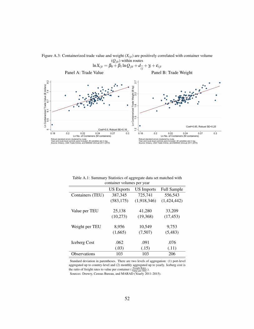
Figure A.3: Containerized trade value and weight (Xi jt ) are positively correlated with container volume(Q jit ) within routes

lnXi jt = β0 +β1 lnQ jit +d↔i j+ γt + εi jt

Panel A: Trade Value

Coef=0.5, Robust SE=0.1655.

56.

16.

77.

48.

2Ln

Con

tain

eriz

ed T

rade

Val

ue (B

dol

lars

)

0.18 0.2 0.22 0.24 0.27 0.3Ln No. of Containers (M containers)

Robust standard errors clustered by route.Year and route level controls were included. All variables are in log.Source: Drewry, USA Trade Online, and MARAD (Annual 2011-2015)

Panel B: Trade Weight

Coef=0.85, Robust SE=0.25

1.2

1.5

1.8

2.2

2.7

Ln C

onta

iner

ized

Tra

de W

eigh

t (B

kg)

0.18 0.2 0.22 0.24 0.27 0.3Ln No. of Containers (M containers)

Robust standard errors clustered by route.Year and route level controls were included. All variables are in log.Source: Drewry, USA Trade Online, and MARAD (Annual 2011-2015)

Table A.1: Summary Statistics of aggregate data set matched withcontainer volumes per year

US Exports US Imports Full SampleContainers (TEU) 387,345 725,741 556,543

(583,175) (1,918,346) (1,424,442)

Value per TEU 25,138 41,280 33,209(10,273) (19,368) (17,453)

Weight per TEU 8,956 10,549 9,753(1,665) (7,507) (5,483)

Iceberg Cost .062 .091 .076(.03) (.15) (.11)

Observations 103 103 206Standard deviation in parentheses. There are two levels of aggregation: (1) port-level

aggregated up to country-level and (2) monthly aggregated up to yearly. Iceberg cost isthe ratio of freight rates to value per container ( Freight Rates

Value per TEU ).Sources: Drewry, Census Bureau, and MARAD (Yearly 2011-2015).

52

Table A.2: Regression of container freight rate within port-pairs

(1) (2)ln Freight Rates ln Freight Rates

ln Opposite Dir FR -0.205∗ -0.814∗∗∗

(0.0778) (0.0202)

ln Distance 0.587∗∗∗

(0.0718)Observations 4033 4033Route FE YTime FE Y YR2 0.235 0.818F 34.52 1620.6Route-level clustered standard errors (SE) in parentheses.

* p < 0.05, ** p < 0.01, *** p < 0.001

(1) has distance and time controls while (2) has route and time controls.

Sources: Drewry and sea-distances.org (Monthly 2006-Jun 2016)

Figure A.4: Tariff rates are mostly constant for country pairs during my sample period

020

4060

80Pe

rcen

t

0 .25 .5 .75 1 1.25 1.5Average annual percentage point change by country pair

Average change is 0.18 percentage points (sd 0.29).Effectively applied average tariff rates for manufactures (average tariff is 4.2%, sd 3%).Source: World Integrated Trade Solution (WITS), World Bank (Annual 2011-2016)

53

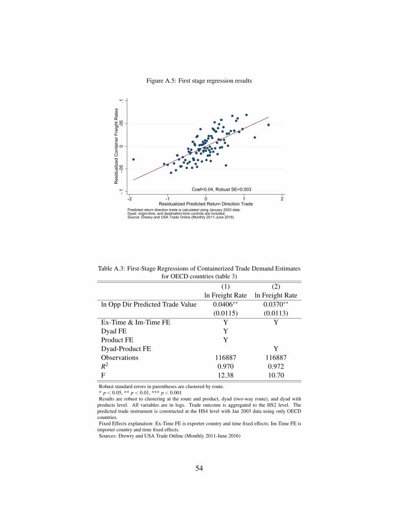
Figure A.5: First stage regression results

Coef=0.04, Robust SE=0.003

-.1-.0

50

.05

.1R

esid

ualiz

ed C

onta

iner

Fre

ight

Rat

es

-2 -1 0 1 2Residualized Predicted Return Direction Trade

Predicted return direction trade is calculated using January 2003 data.Dyad, origin-time, and destination-time controls are included.Source: Drewry and USA Trade Online (Monthly 2011-June 2016)

Table A.3: First-Stage Regressions of Containerized Trade Demand Estimatesfor OECD countries (table 3)

(1) (2)ln Freight Rate ln Freight Rate

ln Opp Dir Predicted Trade Value 0.0406∗∗ 0.0370∗∗

(0.0115) (0.0113)Ex-Time & Im-Time FE Y YDyad FE YProduct FE YDyad-Product FE YObservations 116887 116887R2 0.970 0.972F 12.38 10.70

Robust standard errors in parentheses are clustered by route.* p < 0.05, ** p < 0.01, *** p < 0.001Results are robust to clustering at the route and product, dyad (two-way route), and dyad with

products level. All variables are in logs. Trade outcome is aggregated to the HS2 level. Thepredicted trade instrument is constructed at the HS4 level with Jan 2003 data using only OECDcountries.Fixed Effects explanation: Ex-Time FE is exporter country and time fixed effects; Im-Time FE is

importer country and time fixed effects.Sources: Drewry and USA Trade Online (Monthly 2011-June 2016)

54

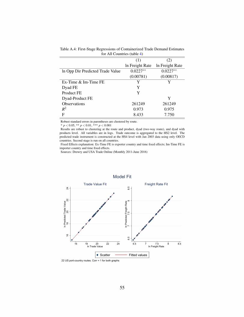
Table A.4: First-Stage Regressions of Containerized Trade Demand Estimatesfor All Countries (table 4)

(1) (2)ln Freight Rate ln Freight Rate

ln Opp Dir Predicted Trade Value 0.0227∗∗ 0.0227∗∗

(0.00781) (0.00817)Ex-Time & Im-Time FE Y YDyad FE YProduct FE YDyad-Product FE YObservations 261249 261249R2 0.973 0.975F 8.433 7.750

Robust standard errors in parentheses are clustered by route.* p < 0.05, ** p < 0.01, *** p < 0.001Results are robust to clustering at the route and product, dyad (two-way route), and dyad with

products level. All variables are in logs. Trade outcome is aggregated to the HS2 level. Thepredicted trade instrument is constructed at the HS4 level with Jan 2003 data using only OECDcountries. Second stage is run on all countries.Fixed Effects explanation: Ex-Time FE is exporter country and time fixed effects; Im-Time FE is

importer country and time fixed effects.Sources: Drewry and USA Trade Online (Monthly 2011-June 2016)

Figure A.6: Model fit

1618

2022

24ln

Pre

dict

ed T

rade

Val

ue

16 18 20 22 24ln Trade Value

Trade Value Fit

6.5

77.

58

8.5

ln P

redi

cted

Fre

ight

Rat

e

6.5 7 7.5 8 8.5ln Freight Rate

Freight Rate Fit

22 US port-country routes. Corr = 1 for both graphs

Model Fit

Scatter Fitted values

55

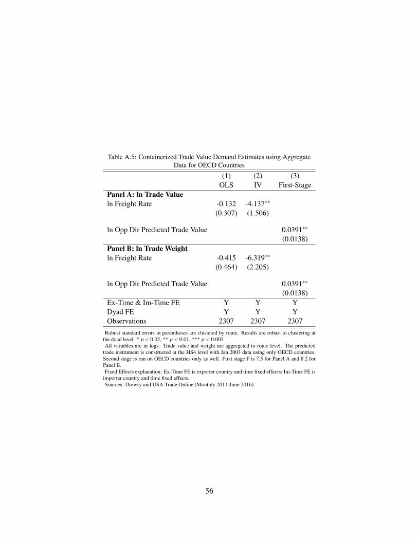
Table A.5: Containerized Trade Value Demand Estimates using AggregateData for OECD Countries

(1) (2) (3)OLS IV First-Stage

Panel A: ln Trade Valueln Freight Rate -0.132 -4.137∗∗

(0.307) (1.506)

ln Opp Dir Predicted Trade Value 0.0391∗∗

(0.0138)Panel B: ln Trade Weightln Freight Rate -0.415 -6.319∗∗

(0.464) (2.205)

ln Opp Dir Predicted Trade Value 0.0391∗∗

(0.0138)Ex-Time & Im-Time FE Y Y YDyad FE Y Y YObservations 2307 2307 2307

Robust standard errors in parentheses are clustered by route. Results are robust to clustering atthe dyad level. * p < 0.05, ** p < 0.01, *** p < 0.001All variables are in logs. Trade value and weight are aggregated to route level. The predicted

trade instrument is constructed at the HS4 level with Jan 2003 data using only OECD countries.Second stage is run on OECD countries only as well. First stage F is 7.5 for Panel A and 8.2 forPanel B.Fixed Effects explanation: Ex-Time FE is exporter country and time fixed effects; Im-Time FE is

importer country and time fixed effects.Sources: Drewry and USA Trade Online (Monthly 2011-June 2016)

56

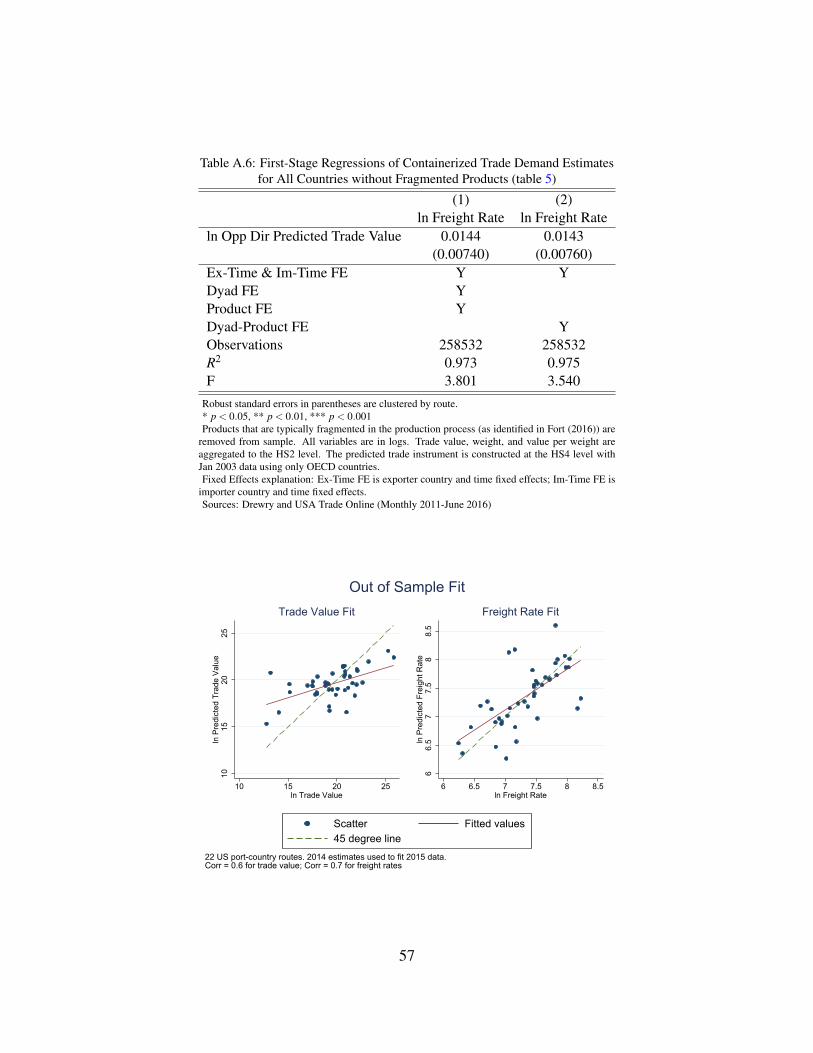
Table A.6: First-Stage Regressions of Containerized Trade Demand Estimatesfor All Countries without Fragmented Products (table 5)

(1) (2)ln Freight Rate ln Freight Rate

ln Opp Dir Predicted Trade Value 0.0144 0.0143(0.00740) (0.00760)

Ex-Time & Im-Time FE Y YDyad FE YProduct FE YDyad-Product FE YObservations 258532 258532R2 0.973 0.975F 3.801 3.540

Robust standard errors in parentheses are clustered by route.* p < 0.05, ** p < 0.01, *** p < 0.001Products that are typically fragmented in the production process (as identified in Fort (2016)) are

removed from sample. All variables are in logs. Trade value, weight, and value per weight areaggregated to the HS2 level. The predicted trade instrument is constructed at the HS4 level withJan 2003 data using only OECD countries.Fixed Effects explanation: Ex-Time FE is exporter country and time fixed effects; Im-Time FE is

importer country and time fixed effects.Sources: Drewry and USA Trade Online (Monthly 2011-June 2016)

Figure A.7: Out of Sample Fit

1015

2025

ln P

redi

cted

Tra

de V

alue

10 15 20 25ln Trade Value

Trade Value Fit

66.

57

7.5

88.

5ln

Pre

dict

ed F

reig

ht R

ate

6 6.5 7 7.5 8 8.5ln Freight Rate

Freight Rate Fit

22 US port-country routes. 2014 estimates used to fit 2015 data.Corr = 0.6 for trade value; Corr = 0.7 for freight rates

Out of Sample Fit

Scatter Fitted values45 degree line

57

Table A.7: Containerized Trade Demand Estimates for OECD Countries with 2009 instrument

(1) (2) (3) (4)OLS OLS IV IV

Panel A: ln Trade Valueln Freight Rate -0.640∗∗∗ -0.503∗∗∗ -1.919∗ -1.044

(0.147) (0.131) (0.715) (0.670)

Panel B: ln Trade Weightln Freight Rate -1.014∗∗∗ -0.808∗∗∗ -2.436∗∗ -1.302

(0.195) (0.175) (0.878) (0.778)

Panel C: ln Trade Value per Weightln Freight Rate 0.374∗∗∗ 0.305∗∗∗ 0.518∗ 0.258

(0.0688) (0.0675) (0.200) (0.185)

Ex-Time & Im-Time FE Y Y Y YDyad FE Y YProduct FE Y YDyad-Product FE Y YObservations 118030 118030 118030 118030First Stage F 27.12 26.43

Robust standard errors in parentheses are clustered by route. * p < 0.05, ** p < 0.01, *** p < 0.001Results are robust to clustering at the route and products, dyad (two-way route), as well as dyad with product levels.

All variables are in logs. Trade outcome is aggregated to the HS2 level. Table A.8 presents the first stage regressions.The predicted trade instrument is constructed at the HS4 level with Jan 2009 data using only OECD countries.Fixed Effects explanation: Ex-Time FE is exporter country and time fixed effects and Im-Time FE is importer country

and time fixed effects.Sources: Drewry and USA Trade Online (Monthly 2011-June 2016)

58

Table A.8: First-Stage Regressions of Containerized Trade Demand Estimatesfor OECD Countries with 2009 instrument (table A.7)

(1) (2)ln Freight Rate ln Freight Rate

ln Opp Dir Predicted Trade Value 0.0511∗∗∗ 0.0485∗∗∗

(0.00981) (0.00943)Ex-Time & Im-Time FE Y YDyad FE YProduct FE YDyad-Product FE YObservations 118030 118030R2 0.971 0.973F 27.12 26.43

Robust standard errors in parentheses are clustered by route.* p < 0.05, ** p < 0.01, *** p < 0.001Results are robust to clustering at the route and product, dyad (two-way route), and dyad with

products level. All variables are in logs. Trade value is aggregated to the HS2 level.The predicted trade instrument is constructed at the HS4 level with Jan 2009 data using only

OECD countries.Fixed Effects explanation: Ex-Time FE is exporter country and time fixed effects; Im-Time FE is

importer country and time fixed effects; Prod-Ex-T FE is product, exporter country, and time fixedeffects; Prod-Im-T FE is product, importer country, and time fixed effects.Sources: Drewry and USA Trade Online (Monthly 2011-June 2016)

59

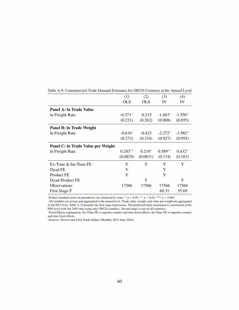
Table A.9: Containerized Trade Demand Estimates for OECD Countries at the Annual Level

(1) (2) (3) (4)OLS OLS IV IV

Panel A: ln Trade Valueln Freight Rate -0.373+ -0.215 -1.683∗ -1.550+

(0.221) (0.262) (0.808) (0.855)

Panel B: ln Trade Weightln Freight Rate -0.616∗ -0.433 -2.272∗ -1.982∗

(0.273) (0.314) (0.927) (0.955)

Panel C: ln Trade Value per Weightln Freight Rate 0.243∗∗ 0.218∗ 0.589∗∗ 0.432∗

(0.0829) (0.0831) (0.174) (0.183)

Ex-Time & Im-Time FE Y Y Y YDyad FE Y YProduct FE Y YDyad-Product FE Y YObservations 17566 17566 17566 17566First Stage F 68.31 55.69

Robust standard errors in parentheses are clustered by route. * p < 0.05, ** p < 0.01, *** p < 0.001All variables are in logs and aggregated to the annual level. Trade value, weight, and value per weight are aggregated

to the HS2 level. Table A.10 presents the first stage regressions. The predicted trade instrument is constructed at theHS4 level with Jan 2003 data using only OECD countries. Second stage is run on all countries.Fixed Effects explanation: Ex-Time FE is exporter country and time fixed effects; Im-Time FE is importer country

and time fixed effects.Sources: Drewry and USA Trade Online (Monthly 2011-June 2016)

60

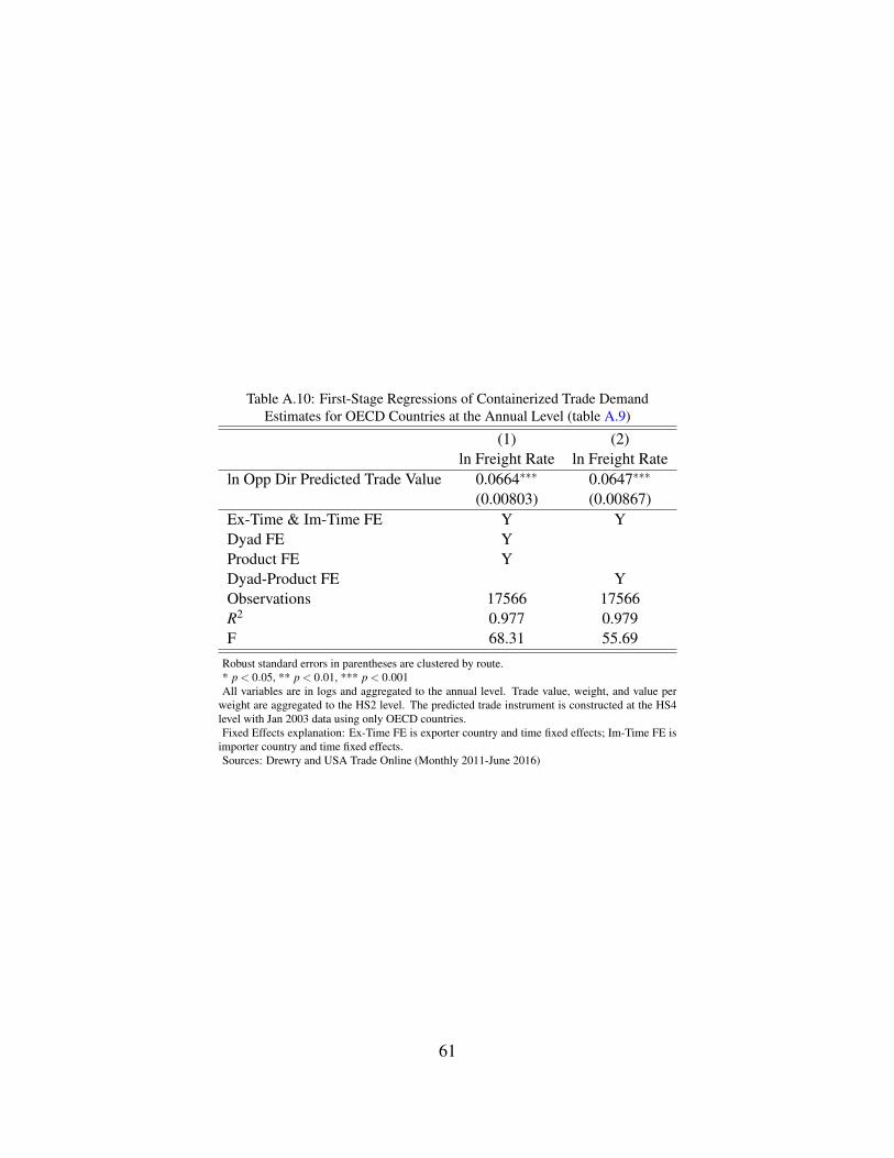
Table A.10: First-Stage Regressions of Containerized Trade DemandEstimates for OECD Countries at the Annual Level (table A.9)

(1) (2)ln Freight Rate ln Freight Rate

ln Opp Dir Predicted Trade Value 0.0664∗∗∗ 0.0647∗∗∗

(0.00803) (0.00867)Ex-Time & Im-Time FE Y YDyad FE YProduct FE YDyad-Product FE YObservations 17566 17566R2 0.977 0.979F 68.31 55.69

Robust standard errors in parentheses are clustered by route.* p < 0.05, ** p < 0.01, *** p < 0.001All variables are in logs and aggregated to the annual level. Trade value, weight, and value per

weight are aggregated to the HS2 level. The predicted trade instrument is constructed at the HS4level with Jan 2003 data using only OECD countries.Fixed Effects explanation: Ex-Time FE is exporter country and time fixed effects; Im-Time FE is

importer country and time fixed effects.Sources: Drewry and USA Trade Online (Monthly 2011-June 2016)

61

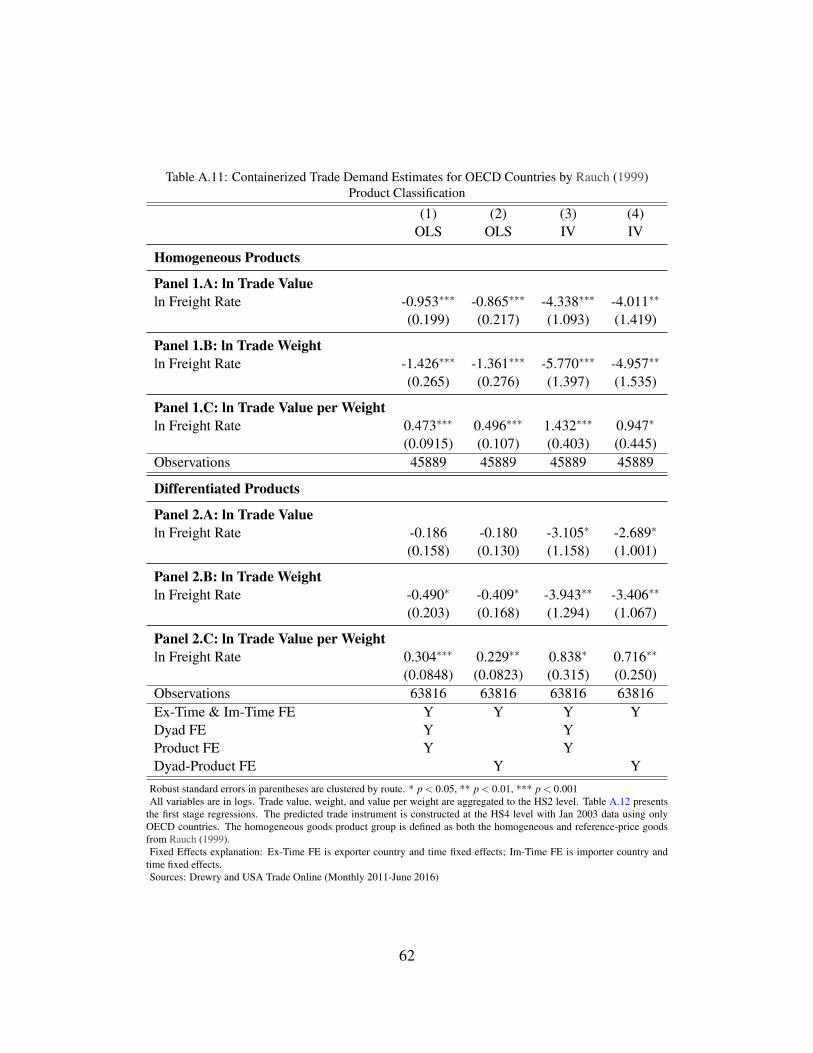
Table A.11: Containerized Trade Demand Estimates for OECD Countries by Rauch (1999)Product Classification

(1) (2) (3) (4)OLS OLS IV IV

Homogeneous Products

Panel 1.A: ln Trade Valueln Freight Rate -0.953∗∗∗ -0.865∗∗∗ -4.338∗∗∗ -4.011∗∗

(0.199) (0.217) (1.093) (1.419)

Panel 1.B: ln Trade Weightln Freight Rate -1.426∗∗∗ -1.361∗∗∗ -5.770∗∗∗ -4.957∗∗

(0.265) (0.276) (1.397) (1.535)

Panel 1.C: ln Trade Value per Weightln Freight Rate 0.473∗∗∗ 0.496∗∗∗ 1.432∗∗∗ 0.947∗

(0.0915) (0.107) (0.403) (0.445)Observations 45889 45889 45889 45889

Differentiated Products

Panel 2.A: ln Trade Valueln Freight Rate -0.186 -0.180 -3.105∗ -2.689∗

(0.158) (0.130) (1.158) (1.001)

Panel 2.B: ln Trade Weightln Freight Rate -0.490∗ -0.409∗ -3.943∗∗ -3.406∗∗

(0.203) (0.168) (1.294) (1.067)

Panel 2.C: ln Trade Value per Weightln Freight Rate 0.304∗∗∗ 0.229∗∗ 0.838∗ 0.716∗∗

(0.0848) (0.0823) (0.315) (0.250)Observations 63816 63816 63816 63816Ex-Time & Im-Time FE Y Y Y YDyad FE Y YProduct FE Y YDyad-Product FE Y Y

Robust standard errors in parentheses are clustered by route. * p < 0.05, ** p < 0.01, *** p < 0.001All variables are in logs. Trade value, weight, and value per weight are aggregated to the HS2 level. Table A.12 presents

the first stage regressions. The predicted trade instrument is constructed at the HS4 level with Jan 2003 data using onlyOECD countries. The homogeneous goods product group is defined as both the homogeneous and reference-price goodsfrom Rauch (1999).Fixed Effects explanation: Ex-Time FE is exporter country and time fixed effects; Im-Time FE is importer country and

time fixed effects.Sources: Drewry and USA Trade Online (Monthly 2011-June 2016)

62

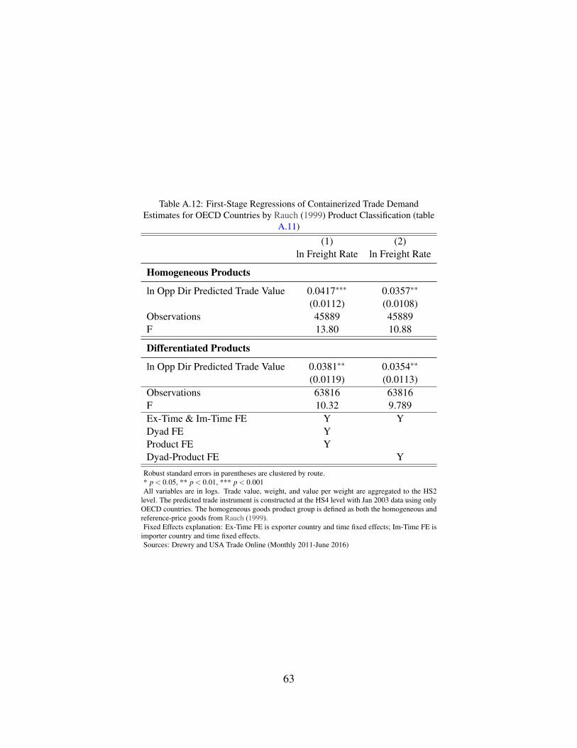
Table A.12: First-Stage Regressions of Containerized Trade DemandEstimates for OECD Countries by Rauch (1999) Product Classification (table

A.11)

(1) (2)ln Freight Rate ln Freight Rate

Homogeneous Products

ln Opp Dir Predicted Trade Value 0.0417∗∗∗ 0.0357∗∗

(0.0112) (0.0108)Observations 45889 45889F 13.80 10.88

Differentiated Products

ln Opp Dir Predicted Trade Value 0.0381∗∗ 0.0354∗∗

(0.0119) (0.0113)Observations 63816 63816F 10.32 9.789Ex-Time & Im-Time FE Y YDyad FE YProduct FE YDyad-Product FE Y

Robust standard errors in parentheses are clustered by route.* p < 0.05, ** p < 0.01, *** p < 0.001All variables are in logs. Trade value, weight, and value per weight are aggregated to the HS2

level. The predicted trade instrument is constructed at the HS4 level with Jan 2003 data using onlyOECD countries. The homogeneous goods product group is defined as both the homogeneous andreference-price goods from Rauch (1999).Fixed Effects explanation: Ex-Time FE is exporter country and time fixed effects; Im-Time FE is

importer country and time fixed effects.Sources: Drewry and USA Trade Online (Monthly 2011-June 2016)

63

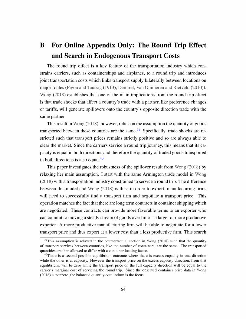
B For Online Appendix Only: The Round Trip Effectand Search in Endogenous Transport Costs

The round trip effect is a key feature of the transportation industry which con-strains carriers, such as containerships and airplanes, to a round trip and introducesjoint transportation costs which links transport supply bilaterally between locations onmajor routes (Pigou and Taussig (1913), Demirel, Van Ommeren and Rietveld (2010)).Wong (2018) establishes that one of the main implications from the round trip effectis that trade shocks that affect a country’s trade with a partner, like preference changesor tariffs, will generate spillovers onto the country’s opposite direction trade with thesame partner.

This result in Wong (2018), however, relies on the assumption the quantity of goodstransported between these countries are the same.39 Specifically, trade shocks are re-stricted such that transport prices remains strictly positive and so are always able toclear the market. Since the carriers service a round trip journey, this means that its ca-pacity is equal in both directions and therefore the quantity of traded goods transportedin both directions is also equal.40

This paper investigates the robustness of the spillover result from Wong (2018) byrelaxing her main assumption. I start with the same Armington trade model in Wong(2018) with a transportation industry constrained to service a round trip. The differencebetween this model and Wong (2018) is this: in order to export, manufacturing firmswill need to successfully find a transport firm and negotiate a transport price. Thisoperation matches the fact that there are long term contracts in container shipping whichare negotiated. These contracts can provide more favorable terms to an exporter whocan commit to moving a steady stream of goods over time—a larger or more productiveexporter. A more productive manufacturing firm will be able to negotiate for a lowertransport price and thus export at a lower cost than a less productive firm. This search

39This assumption is relaxed in the counterfactual section in Wong (2018) such that the quantityof transport services between countries, like the number of containers, are the same. The transportedquantities are then allowed to differ with a container loading factor.

40There is a second possible equilibrium outcome where there is excess capacity in one directionwhile the other is at capacity. However the transport price on the excess capacity direction, from thatequilibrium, will be zero while the transport price on the full capacity direction will be equal to thecarrier’s marginal cost of servicing the round trip. Since the observed container price data in Wong(2018) is nonzero, the balanced quantity equilibrium is the focus.

64

process smooths the relationship between price and quantity relative to the trade shockswhich renders the balanced quantity assumption unnecessary.

This paper shows that the main spillover predictions from Wong (2018) hold with-out the balanced trade assumption. An increase in a country’s tariffs on its tradingpartner’s good will result in an increase in the country’s export transport costs to thesame partner. This is because the decrease in the country’s imports due to its tariff risewill result in less incoming transport firms. From the round trip effect, the number ofoutgoing transport firms will decrease as well. However, since the partner’s demandfor the country’s exports have not changed, the fall in transport supply will result in arelative rise in export transport costs which decreases its equilibrium export quantityand value to the partner it was imposing protectionist policies on. On the flip side, anincrease in a country’s preferences for its trading partner’s good will result in a decreasein the country’s export transport cost to the same partner and an increase in its exportquantity and value to the same. This result provides evidence for the robust relationshipbetween the round trip effect and the spillover of shocks between a country’s two-waytrade with one particular trading partner via transport costs.

The first section describes the model setup and its five stages. Sections 2 to 6highlight each stage respectively. Section 7 characterizes the equilibrium and section 8presents the main predictions of the model. Section 9 concludes.

B.1 Model SetupThe trade model is an augmented partial equilibrium Armington model with multi-

ple countries from Hummels, Lugovskyy and Skiba (2009) with three types of agents:consumers, manufacturing firms, and transport firms.41 Consumers in each countrymaximize utility by consuming two types of goods—a differentiated good that can beproduced locally or abroad as well as a homogeneous local good. Countries are hetero-geneous and each has one manufacturing firm which produces a unique manufacturingvariety and prices like a monopolistically competitive firm. These firms choose pro-duction to just meet local demand or to export as well. If they export, they requirea transport firm to ship their goods to the destination country. The firm will need to

41The theory model in Wong (2018) introduces three modifications. The first is the incorporation ofthe round trip constraint into the transport firm’s profit function. Second, countries are allowed to beheterogeneous. Third, perfectly competitive transport firms are assumed. The fourth novel modificationin this paper is the inclusion of a search and bargaining process between manufacturing and transportfirms.

65

successfully find a transportation firm and negotiate a transport price in order to export.This operation is modeled as a search and bargaining process between the exportingmanufacturing firm and the transport firm.

The transport firms are homogeneous and perfectly competitive. The round tripeffect applies to these firms in that they have to commit to a round trip service if theyenter the market. This is due to the fact that the vessels, trucks, and airplanes utilized bytransport firms are re-used and so have to return to the origin so that they can continueto provide transportation services. In the model, this translates into their joint profits inboth direction being non-negative.

There are five stages in this model:

1. Entry decision of the transport firms (carriers). Since carriers commit to servicinga round trip route upon entry, they will enter the market only if their expectedjoint profits in both directions are non-negative.

2. Export decision of the manufacturing firms (exporters). Upon receiving theirproductivity draw, a manufacturing firm will choose to export or not based ontheir expected profits from selling the variety as well as going through the searchprocess.

3. Export production decision of the firms. An exporter whose productivity is abovethe export threshold from the previous stage will produce to maximize its exportprofits.

4. Search and bargaining process between exporters and carriers. An exporter needsto successfully search for a carrier and bargain with them for their services inorder to export. Exporters who are unsuccessful will not be able to sell theirgoods but will still have to pay for production costs.

5. Consumers maximize utility by consuming a mixture of locally produced andimported differentiated goods as well as a homogeneous good subject to a budgetconstraint.

Hummels, Lugovskyy and Skiba (2009) is the basis for manufacturing firms andconsumers while Miao (2006) is the basis for the search and bargaining model betweenexporters and carriers. This model is solved by backward induction and each stage ofthe model is introduced below.

66

B.2 Consumer demandI assume that the world consists of M potentially heterogeneous countries where

each country produces a different variety (ω) of a tradeable good.42 Consumers con-sume varieties of the tradeable good from this set of countries as well as a homogeneousnumeraire good. The quasilinear utility function of a representative consumer in coun-try j is

U j = q j0 +∫ M

ai jqi j(ω)(σ−1)/σ dω, σ > 1 (26)

where q j0 is the quantity of the numeraire good consumed by country j, ai j is j’spreference for the variety from country i,43 qi j the quantity of variety consumed onroute i j, while σ is the price elasticity of demand.44 The numeraire good, interpretedas services here, is costlessly traded and its price is normalized to one.

B.3 Transport cost determinationIn order for exporters in i to export qi j amount of its goods to country j, they need

to engage the transport services of the carrier. This is modeled as a process of search,matching, and bargaining in a decentralized market. Once a match occurs, the exporterand carrier will bargain over the price of the transport service, ti j.

The object of bargain here–transportation services–deserve some explanation. Itis not one container since most exporters ship more than one container. It is also notan entire ship since an average exporter does not ship 4000 containers–the averagecapacity of a containership. The reality is somewhere in between. As such, this modeladopts the same interpretation as Wong (2018)—the object of bargain is a shipment ofgoods that includes all the products that an exporter exports to one particular country.For example if there is a exporter who wants to export 5 containers worth of goods fromi to j, she will search for a carrier who is going from i to j. They negotiate for the priceof the 5 container shipment and the export takes place if the negotiation is successful.A carrier picks its round trip capacity to be larger of its shipments within a round trip.

Exporters are heterogeneous, monopolistically competitive, and each produces one

42There is one exporter per country and so the good variety ω translates into the productivity draw ofthe exporter firm ϕ .

43Preference parameter ai j can also be interpreted as the attractiveness of country i’s product to countryj (Head and Mayer (2014)).

44Similar to Hummels, Lugovskyy and Skiba (2009), σ is the price elasticity of demand: ∂qi j∂ pi j

qi jpi j

=−σ

(equation (26)).

67

variety.45 Carrier are homogeneous and incur cost ψi j of transporting a shipment whichis independent of quantity. Examples of this cost include the loading and unloadingcost, the cost of hiring a captain and crew, as well as the capital cost of deploying aship. There are MEx,i j number of exporters and MC,i j number of carriers which areendogenously determined in equilibrium.

There are two frictions in the search process for a trader, who can be an exporteror carrier. First, there is a positive discount rate of r ∈ (0,1]. Second, search incursan explicit cost ρ > 0. Following Miao (2006), it is assumed that a trader contactsanother trader according to a Poisson process with intensity ρ . A trader is a carrier withprobability ζi j(ϕi j) =

MC,i jMC,i j+MEx,i j

where ϕi j is the exporter’s productivity threshold forsearch. An exporter whose productivity is ϕi j will be indifferent between exporting—which necessitates searching for a carrier—and not.

At any time, an exporter with productivity ϕ meets a carrier with probability ρζ (ϕi j).If she can negotiate and agree on a price with the carrier, she can export her goods andobtain her producer surplus in the form of export revenue minus transport cost (ti j),[(

pi j(ϕ)− ti j(ϕ))

qi j(ϕ))].46 If not, the goods expire and are not sold.47 A carrier

meets an exporter with probability ρ(1−ζi j(ϕi j)). If his negotiations with the exporteris successful, he sells his services for ti j(ϕ) and receives a profit of

(ti j(ϕ)qi j(ϕ)−ψi j

).

The carrier’s revenue increases with the amount of goods he transports in one shipment.If the bargaining is unsuccessful, he gets zero profit.

When a exporter meets a carrier, they negotiate a transport price where one of thetwo randomly announces a take-it-or-leave-it price offer. If the offer is accepted, thetrade occurs and they leave the market. If the offer is rejected, the exporter continuessearching. Let VEx,i j(ϕ) be the expected payoff of an exporter with productivity ϕ andVC,i j be the expected payoff of a carrier. The bargaining problem between exporter and

45Following Chaney (2008) and Melitz (2003), exporters are heterogeneous in their productivity (as-sume Pareto distribution G(ϕ) = P(ϕ∗ < ϕ) of productivity ϕ with shape parameter γ ∼ [1,+∞).

46Note that including tariffs in the producer surplus would be straightforward. It would involve addinganother term after transport cost and since tariffs are exogenous here its comparative statics would bethe same as assuming exogenous transport cost. If tariffs from i to j are τi j, the producer surplus is[(pi j(ϕ)− ti j(ϕ)− τi j)qi j(ϕ))].

47The inability of exporters to sell their goods if the search is unsuccessful is a simplification. Anearlier version of this model allows for unsuccessful exporters to sell their goods locally. The end resultbetween the earlier model and the present version is qualitatively similar. The present version is chosenfor simplicity.

68

carrier is as follows:

maxti j

[(pi j(ϕ)− ti j(ϕ)

)qi j(ϕ)−VEx,i j(ϕ)

]η [ti j(ϕ)qi j(ϕ)−ψi j−VC,i j]1−η

where pi j is the per unit price of the export goods, ti j is the per unit transport price, qi j

is the quantity of exports, ψi j is the cost to transport the goods,48 and η ∈ (0,1) is therelative bargaining power of the exporter. This bargaining problem is subject to the factthat exporters and carriers are risk-neutral and enter the market if their expected payoffis positive and only if their expected payoff is non-negative,

(pi j(ϕ)− ti j(ϕ)

)qi j(ϕ)≥

VEx,i j(ϕ) and ti j(ϕ)qi j(ϕ)−ψi j ≥ VC,i j. As such, the transport price for one unit ofgood is as follows:

ti j(ϕ) =1

qi j(ϕ)

[η(ψi j +VC,i j

)+(1−η)

(pi j(ϕ)qi j(ϕ)−VEx,i j(ϕ)

)](27)

where the transport price is increasing in the cost of providing transport services (ψi j),the exporter’s relative bargaining power (η), as well as the expected payoff of the car-riers (VC,i). It is decreasing in the relative bargaining power of the carriers (1−η) andthe expected payoff of the exporters (VEx,i). The effect of export quantity qi j(ϕ) ontransport price depends on the bargaining parameters, cost of shipping, and magnitudesof the value functions.49

The value function of the exporter’s search process (VEx,i j) conditional on its pro-ductivity ϕ being above the search threshold ϕ ≥ ϕi j, is:

rVEx,i(ϕ, ϕi j) = ρζi j(ϕi j)max{[(

pi j(ϕ)− ti j(ϕ))

qi j(ϕ)−VEx,i j(ϕ)],0}

(28)

where the probability of meeting a carrier is ρζ (ϕi j) and the exporter’s total profit fromexporting is the difference between its export revenue and transport cost,

(pi j(ϕ)− ti j(ϕ)

)qi j(ϕ).50

The value function of the carrier VC,i j is as follows:

rVC,i j(ϕi j) = ρ(1−ζi j(ϕi j))EF[max

{[ti j(ϕ)qi j(ϕ)−ψi j−VC,i

],0}]

(29)

where ρ(1− ζi j(ϕi j)) is the probability of a carrier meeting an exporter, and the car-rier’s expected profits is the difference between its revenue and its cost from providingtransport.

Incorporating the bargaining outcome of the transport price in (27), the exporter

48As mentioned earlier, this cost is independent of quantity. It is possible to include a marginal costof transporting the goods that also depends on quantity and the results would not change.

49 ∂ ti j(ϕ)

∂qi j(ϕ)=

(1−η)VEx,i j(ϕ)−η(ψi j+VC,i j)

qi j(ϕ)2 .50Since exporters have already produced their goods before searching for a carrier, their search value

function does not include production costs of their goods.

69

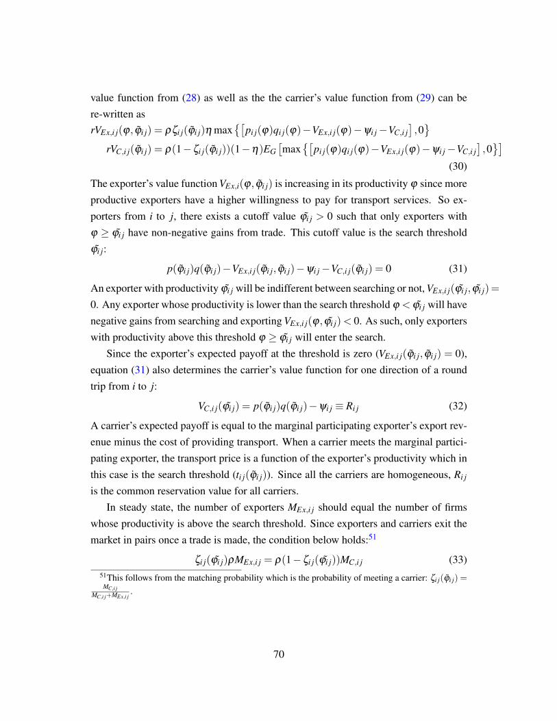
value function from (28) as well as the the carrier’s value function from (29) can bere-written asrVEx,i j(ϕ, ϕi j) = ρζi j(ϕi j)η max

{[pi j(ϕ)qi j(ϕ)−VEx,i j(ϕ)−ψi j−VC,i j

],0}

rVC,i j(ϕi j) = ρ(1−ζi j(ϕi j))(1−η)EG[max

{[pi j(ϕ)qi j(ϕ)−VEx,i j(ϕ)−ψi j−VC,i j

],0}]

(30)

The exporter’s value function VEx,i(ϕ, ϕi j) is increasing in its productivity ϕ since moreproductive exporters have a higher willingness to pay for transport services. So ex-porters from i to j, there exists a cutoff value ϕi j > 0 such that only exporters withϕ ≥ ϕi j have non-negative gains from trade. This cutoff value is the search thresholdϕi j:

p(ϕi j)q(ϕi j)−VEx,i j(ϕi j, ϕi j)−ψi j−VC,i j(ϕi j) = 0 (31)

An exporter with productivity ϕi j will be indifferent between searching or not, VEx,i j(ϕi j, ϕi j)=

0. Any exporter whose productivity is lower than the search threshold ϕ < ϕi j will havenegative gains from searching and exporting VEx,i j(ϕ, ϕi j)< 0. As such, only exporterswith productivity above this threshold ϕ ≥ ϕi j will enter the search.

Since the exporter’s expected payoff at the threshold is zero (VEx,i j(ϕi j, ϕi j) = 0),equation (31) also determines the carrier’s value function for one direction of a roundtrip from i to j:

VC,i j(ϕi j) = p(ϕi j)q(ϕi j)−ψi j ≡ Ri j (32)

A carrier’s expected payoff is equal to the marginal participating exporter’s export rev-enue minus the cost of providing transport. When a carrier meets the marginal partici-pating exporter, the transport price is a function of the exporter’s productivity which inthis case is the search threshold (ti j(ϕi j)). Since all the carriers are homogeneous, Ri j

is the common reservation value for all carriers.In steady state, the number of exporters MEx,i j should equal the number of firms

whose productivity is above the search threshold. Since exporters and carriers exit themarket in pairs once a trade is made, the condition below holds:51

ζi j(ϕi j)ρMEx,i j = ρ(1−ζi j(ϕi j))MC,i j (33)51This follows from the matching probability which is the probability of meeting a carrier: ζi j(ϕi j) =MC,i j

MC,i j+MEx,i j.

70

B.4 Export productionIn Chaney (2008) and Melitz (2003), there are two trade barriers from the perspec-

tive of an exporter: (1) a fixed cost to export defined in terms of the numeraire, and(2) a variable transport cost, or transport price as introduced in the previous section,ti j(ϕ) that exporters in country i with productivity ϕ have to pay to ship their goods todestination j. In this model, transport cost is modeled as the only trade barrier.52 Eachexporter draws a random unit of productivity ϕ . This draw determines their willing-ness to pay for transport services and hence the transport price ti j(ϕ). In addition, anexporter has to search for its carrier in order to export. From the previous section, theprobability of meeting a carrier is ρζi j(ϕi j) which is a function of the share of carriersin i, ζi j(ϕi j) =

MC,i jMC,i j+MEx,i j

.An exporter with productivity ϕ chooses its export price to maximize domestic and

export profits. An exporter who is productive enough to export will also produce fordomestic consumption. However, it can only export if its goods can be transportedabroad by a carrier. Otherwise, the exporter will not be able to export. In both casesit will still have to pay for production costs since the production decision has alreadybeen made. It is assumed that there are no domestic transport costs (tii = 0). The exportprofit maximization problem for an exporter with productivity ϕ in country i selling tocountry j is as follows:

maxpi j(ϕ)

πi j(ϕ) = VEx,i j(ϕ, ϕi j)︸ ︷︷ ︸Surplus from exportingif search is successful

− ci j(ϕ)qi j(ϕ)︸ ︷︷ ︸Production cost regardless

of search outcome

(34)

where it is made up of two terms. The first term is the surplus from exporting if theexporter successfully finds a carrier. The second term is the marginal cost of productionthat the exporter has to pay in order to produce qi j(ϕ) units of its good. The marginalcost term is made up of the price of the sole input, labor (wages wi), and the exporter’sproductivity:

ci j(ϕ)≡wi

ϕ(35)

52The endogenous transport cost generates the fixed cost to export since it has a fixed cost to providetransport ψi j.

71

B.5 Exporter entry decisionThe entry condition in equation (31) determines the search threshold ϕi j, where

exporters are indifferent between searching or not. Here exporters with productivityϕi j will earn zero profit from exporting and so are indifferent between exporting or not:

π(ϕi j) = 0→VEx,i j(ϕi j, ϕi j) = ci j(ϕi j)qi j(ϕi j) =wi

ϕi jqi j(ϕi j) (36)

In equilibrium, the search threshold and the exporting threshold should be the sameϕi j = ϕi j.

B.6 Carrier entry decisionIn order for the carriers to enter the market, their expected profits from their round

trip service has to be non-negative. This means that for any round trip between i and j,VC,i j and VC, ji has to be non-negative:

VC,i j(ϕi j)+VC, ji(ϕi j)≥ 0 (37)

This means that a carrier could still serve a round trip journey when one directiongenerates negative profits if the other direction makes up for the loss. Since carrierswho enter the market commit to a round trip route, there has to be the same number ofcarriers going from i to j and back

MC,i j = MC, ji (38)

B.7 Solving for the EquilibriumFor the tradeable good, the solution to the consumer’s problem in (26) takes the

CES form:

qi j =

[σ

σ −11

ai jpi j

]−σ

(39)

An increase in j’s preference for i’s good (ai j) will increase its demanded quantitywhile an increase in the export price (pi j) will decrease the quantity.

The exporter’s value function in (30), conditional on its productivity being abovethe search threshold ϕi j, can be rewritten as:

VB,i(ϕ, ϕi j) =ρηζi j(ϕi j)

r+ρηζi j(ϕi j)

[pi j(ϕ)qi j(ϕ)−ψi j−Ri j

], for ϕ ≥ ϕi j (40)

By inserting the rewritten exporter’s value function from (40) into the transport price

72

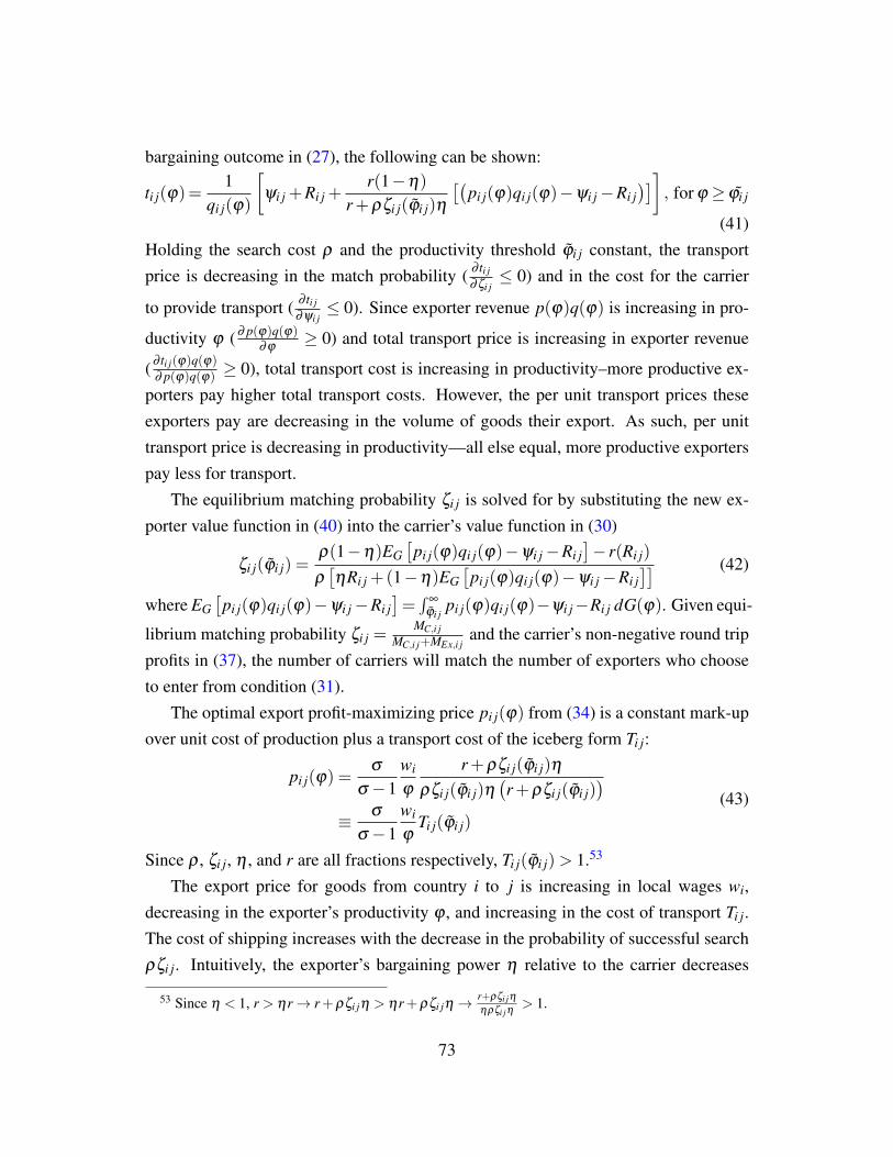
bargaining outcome in (27), the following can be shown:

ti j(ϕ)=1

qi j(ϕ)

[ψi j +Ri j +

r(1−η)

r+ρζi j(ϕi j)η

[(pi j(ϕ)qi j(ϕ)−ψi j−Ri j

)]], for ϕ ≥ ϕi j

(41)Holding the search cost ρ and the productivity threshold ϕi j constant, the transportprice is decreasing in the match probability ( ∂ ti j

∂ζi j≤ 0) and in the cost for the carrier

to provide transport ( ∂ ti j∂ψi j≤ 0). Since exporter revenue p(ϕ)q(ϕ) is increasing in pro-

ductivity ϕ (∂ p(ϕ)q(ϕ)∂ϕ

≥ 0) and total transport price is increasing in exporter revenue

(∂ ti j(ϕ)q(ϕ)∂ p(ϕ)q(ϕ) ≥ 0), total transport cost is increasing in productivity–more productive ex-

porters pay higher total transport costs. However, the per unit transport prices theseexporters pay are decreasing in the volume of goods their export. As such, per unittransport price is decreasing in productivity—all else equal, more productive exporterspay less for transport.

The equilibrium matching probability ζi j is solved for by substituting the new ex-porter value function in (40) into the carrier’s value function in (30)

ζi j(ϕi j) =ρ(1−η)EG

[pi j(ϕ)qi j(ϕ)−ψi j−Ri j

]− r(Ri j)

ρ[ηRi j +(1−η)EG

[pi j(ϕ)qi j(ϕ)−ψi j−Ri j

]] (42)

where EG[pi j(ϕ)qi j(ϕ)−ψi j−Ri j

]=∫

∞

ϕi jpi j(ϕ)qi j(ϕ)−ψi j−Ri j dG(ϕ). Given equi-

librium matching probability ζi j =MC,i j

MC,i j+MEx,i jand the carrier’s non-negative round trip

profits in (37), the number of carriers will match the number of exporters who chooseto enter from condition (31).

The optimal export profit-maximizing price pi j(ϕ) from (34) is a constant mark-upover unit cost of production plus a transport cost of the iceberg form Ti j:

pi j(ϕ) =σ

σ −1wi

ϕ

r+ρζi j(ϕi j)η

ρζi j(ϕi j)η(r+ρζi j(ϕi j)

)≡ σ

σ −1wi

ϕTi j(ϕi j)

(43)

Since ρ , ζi j, η , and r are all fractions respectively, Ti j(ϕi j)> 1.53

The export price for goods from country i to j is increasing in local wages wi,decreasing in the exporter’s productivity ϕ , and increasing in the cost of transport Ti j.The cost of shipping increases with the decrease in the probability of successful searchρζi j. Intuitively, the exporter’s bargaining power η relative to the carrier decreases

53 Since η < 1, r > ηr→ r+ρζi jη > ηr+ρζi jη →r+ρζi jη

ηρζi jη> 1.

73

η → 0, the transport price increases Ti j→ ∞ as does the export price pi j→ ∞.The export profits of an exporter with productivity ϕ > ϕi j from i to j is

πi j(ϕ) =ρζi j(ϕi j)η

(r+ρζi j(ϕi j)

)r+ρζi j(ϕi j)η

[pi j(ϕ)qi j(ϕ)−Ri j−ψi j

]− wi

ϕqi j(ϕ)

=1

Ti j(ϕi j)

[pi j(ϕ)qi j(ϕ)−Ri j−ψi j

]− wi

ϕqi j(ϕ)

(44)

Here a decrease in the transport price (Ti j), wages (wi), carrier’s reservation value (Ri j),and the cost of providing transport services (ψi j) will increase exporter profits. Anincrease in the export revenue (pi j(ϕ)qi j(ϕ)) will also increase profits.

In equilibrium, an exporter’s search threshold is equal to its export threshold: ϕi j =

ϕi j. Hence the export productivity threshold of the exporters (ϕi j) can be pinned downby equating their value function from search (equation (40)) to the cost of productionthat they pay for regardless of the search outcome. This means that the exporter earnszero profit in equation (34):54

πi j(ϕi j) = 0→VEx,i j(ϕi j, ϕi j = ϕi j) = ci j(ϕi j)qi j(ϕi j)

ϕi j = λ1

[Ri j +ψi j

aσi j

] 1σ−1

wiTi j(ϕi j)(45)

Note that this export threshold is not solved in its entirety yet since the transport coststill takes the threshold as a function due to matching probability ζi j(ϕi j). Any manu-facturing firms who draw a productivity lower than this threshold will choose to onlyproduce domestically. All else equal, an increase in the reservation value of the carrier(Ri j), the cost of providing transport (ψi j), the cost of production (wi), and the transportprice (Ti j(ϕi j)) raises the export threshold which lowers the number of exporters. Anincrease in j’s preference for i’s product (ai j) will decrease the export threshold whichincreases the number of exporters.

Between two countries k and l, the equilibrium in this model can be describedby the following (for k, l = i, j and k 6= l): the utility-maximizing quantity of goodstraded back and forth (qkl), value functions of exporters and carriers (VEx,kl and VC,kl),negotiated transport prices (tkl(ϕ)), profit-maximizing prices of goods traded back andforth (pkl(ϕ)), marginal exporters (ϕkl), and the stock of exporters and carriers (MEx,kl

and MC,kl) such that

54Constant λ1 ≡[

σ

σ−1−2σ 1

σ−1

] 1σ−1

74

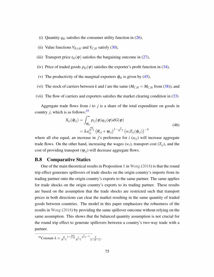
(i) Quantity qkl satisfies the consumer utility function in (26),

(ii) Value functions VEx,kl and VC,kl satisfy (30),

(iii) Transport price tkl(ϕ) satisfies the bargaining outcome in (27),

(iv) Price of traded goods pkl(ϕ) satisfies the exporter’s profit function in (34),

(v) The productivity of the marginal exporters ϕkl is given by (45),

(vi) The stock of carriers between k and l are the same (MC,kl = MC,lk from (38)), and

(vii) The flow of carriers and exporters satisfies the market clearing condition in (33)

Aggregate trade flows from i to j is a share of the total expenditure on goods incountry j, which is as follows:55

Xi j(ϕi j) =∫

∞

¯ϕk j

pi j(ϕ)qi j(ϕ)dG(ϕ)

= λaσγ

σ−1i j(Ri j +ψi j

)1− γ

σ−1(wiTi j(ϕi j)

)−γ

(46)

where all else equal, an increase in j’s preference for i (ai j) will increase aggregatetrade flows. On the other hand, increasing the wages (wi), transport cost (Ti j), and thecost of providing transport (ψi j) will decrease aggregate flows.

B.8 Comparative StaticsOne of the main theoretical results in Proposition 1 in Wong (2018) is that the round

trip effect generates spillovers of trade shocks on the origin country’s imports from itstrading partner onto the origin country’s exports to the same partner. The same appliesfor trade shocks on the origin country’s exports to its trading partner. These resultsare based on the assumption that the trade shocks are restricted such that transportprices in both directions can clear the market resulting in the same quantity of tradedgoods between countries. The model in this paper emphasizes the robustness of theresults in Wong (2018) by providing the same spillover outcome without relying on thesame assumption. This shows that the balanced quantity assumption is not crucial forthe round trip effect to generate spillovers between a country’s two-way trade with apartner.

55Constant λ ≡ σ

σ−11+ 2σγ

1−σ 1σ−1

γ

σ−1−1 γ

γ−(σ−1) .

75

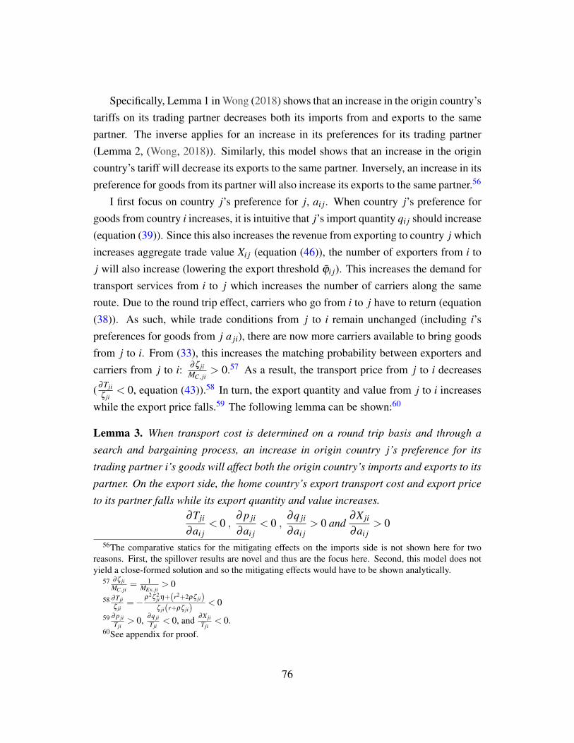
Specifically, Lemma 1 in Wong (2018) shows that an increase in the origin country’stariffs on its trading partner decreases both its imports from and exports to the samepartner. The inverse applies for an increase in its preferences for its trading partner(Lemma 2, (Wong, 2018)). Similarly, this model shows that an increase in the origincountry’s tariff will decrease its exports to the same partner. Inversely, an increase in itspreference for goods from its partner will also increase its exports to the same partner.56

I first focus on country j’s preference for j, ai j. When country j’s preference forgoods from country i increases, it is intuitive that j’s import quantity qi j should increase(equation (39)). Since this also increases the revenue from exporting to country j whichincreases aggregate trade value Xi j (equation (46)), the number of exporters from i toj will also increase (lowering the export threshold ϕi j). This increases the demand fortransport services from i to j which increases the number of carriers along the sameroute. Due to the round trip effect, carriers who go from i to j have to return (equation(38)). As such, while trade conditions from j to i remain unchanged (including i’spreferences for goods from j a ji), there are now more carriers available to bring goodsfrom j to i. From (33), this increases the matching probability between exporters andcarriers from j to i: ∂ζ ji

MC, ji> 0.57 As a result, the transport price from j to i decreases

(∂Tjiζ ji

< 0, equation (43)).58 In turn, the export quantity and value from j to i increaseswhile the export price falls.59 The following lemma can be shown:60

Lemma 3. When transport cost is determined on a round trip basis and through a

search and bargaining process, an increase in origin country j’s preference for its

trading partner i’s goods will affect both the origin country’s imports and exports to its

partner. On the export side, the home country’s export transport cost and export price

to its partner falls while its export quantity and value increases.∂Tji

∂ai j< 0 ,

∂ p ji

∂ai j< 0 ,

∂q ji

∂ai j> 0 and

∂X ji

∂ai j> 0

56The comparative statics for the mitigating effects on the imports side is not shown here for tworeasons. First, the spillover results are novel and thus are the focus here. Second, this model does notyield a close-formed solution and so the mitigating effects would have to be shown analytically.

57 ∂ζ jiMC, ji

= 1MEx, ji

> 0

58 ∂Tjiζ ji

=−ρ2ζ 2jiη+(r2+2ρζ ji)ζ ji(r+ρζ ji)

< 0

59 ∂ p jiTji

> 0, ∂q jiTji

< 0, and ∂X jiTji

< 0.60See appendix for proof.

76

In order to establish these results for tariffs, I first incorporate tariffs into this model.Tariffs are paid by the exporters and so they are incorporated into their profit functionsin (34) as such:

maxpi j(ϕ)

πi j(ϕ) = ρζi j(ϕ, ϕi j)(

pi j(ϕ)− ti j(ϕ))

qi j(ϕ)− τi jci j(ϕ)qi j(ϕ) (47)

where the first two terms are the surplus from being able to export if the exportersuccessfully finds a carrier. The second term is the marginal cost of production thatthe exporter has to pay in order to produce qi j(ϕ) units of its good which includes thetariff on these goods τi j > 1.61 The marginal cost term is made up of the price of thesole input, labor (wi), and the exporter’s productivity. The equilibrium for this modelwith tariffs is very similar to the equilibrium defined previously where tariffs enter thesame way as wages wi.

When country j increases its tariffs on goods from country i, it is again intuitive thatits import price pi j should increase which will lead to a fall in quantity qi j (equation(39)).62 Since this then decreases the revenue from exporting to country j (Xi j, equa-tion (46)), the number of exporters will also fall which increases the export thresholdϕi j. This decreases the demand for transport services from i to j which decreases thenumber of carriers along the same route. Due to the round trip effect, there are nowless carriers available to bring goods from j to i all else equal (equation (38)). From(33), this decreases the matching probability between exporters and carriers from j to i:∂ζ jiMC, ji

> 0. As a result, the transport price from j to i increases (∂Tjiζ ji

< 0, equation (43)).The export quantity and value from j to i falls while price increases. The followinglemma can be shown:63

Lemma 4. When transport cost is determined on a round trip basis and through a

search and bargaining process, an increase in the origin country j’s import tariffs on

its trading partner i’s goods will affect both the origin country’s imports and exports to

its partner. On the export side, the origin country’s export freight rate and price to its

61This method of modeling is chosen for simplicity. Another way to model tariffs here is for the firmsto only pay for it if it successfully exports. This alternative method would not change the results butwould complicate the solution.

62Since pi j(ϕ) =σ

σ−1wiτi j

ϕ

r+ρζi j(ϕi j)η

ρζi j(ϕi j)η(r+ρζi j(ϕi j))≡ σ

σ−1wiτi j

ϕTi j(ϕi j),

∂ p jiτi j<0 .

63See appendix for proof.

77

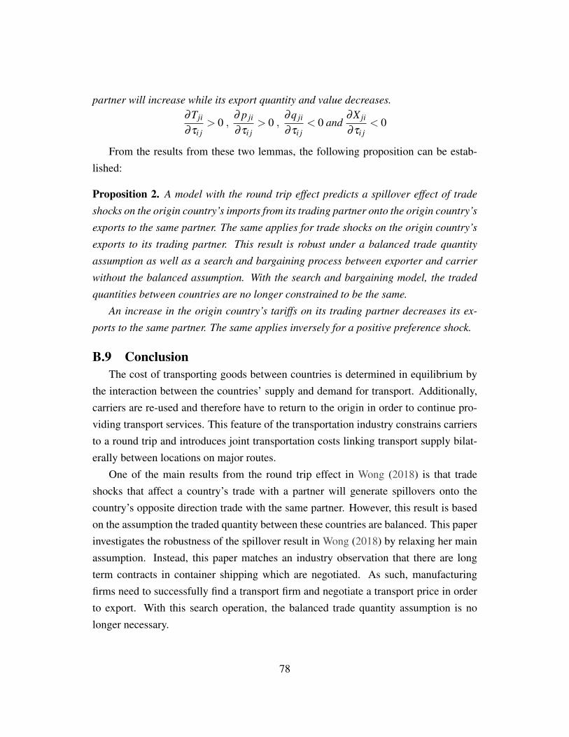
partner will increase while its export quantity and value decreases.∂Tji

∂τi j> 0 ,

∂ p ji

∂τi j> 0 ,

∂q ji

∂τi j< 0 and

∂X ji

∂τi j< 0

From the results from these two lemmas, the following proposition can be estab-lished:

Proposition 2. A model with the round trip effect predicts a spillover effect of trade

shocks on the origin country’s imports from its trading partner onto the origin country’s

exports to the same partner. The same applies for trade shocks on the origin country’s

exports to its trading partner. This result is robust under a balanced trade quantity

assumption as well as a search and bargaining process between exporter and carrier

without the balanced assumption. With the search and bargaining model, the traded

quantities between countries are no longer constrained to be the same.

An increase in the origin country’s tariffs on its trading partner decreases its ex-

ports to the same partner. The same applies inversely for a positive preference shock.

B.9 ConclusionThe cost of transporting goods between countries is determined in equilibrium by

the interaction between the countries’ supply and demand for transport. Additionally,carriers are re-used and therefore have to return to the origin in order to continue pro-viding transport services. This feature of the transportation industry constrains carriersto a round trip and introduces joint transportation costs linking transport supply bilat-erally between locations on major routes.

One of the main results from the round trip effect in Wong (2018) is that tradeshocks that affect a country’s trade with a partner will generate spillovers onto thecountry’s opposite direction trade with the same partner. However, this result is basedon the assumption the traded quantity between these countries are balanced. This paperinvestigates the robustness of the spillover result in Wong (2018) by relaxing her mainassumption. Instead, this paper matches an industry observation that there are longterm contracts in container shipping which are negotiated. As such, manufacturingfirms need to successfully find a transport firm and negotiate a transport price in orderto export. With this search operation, the balanced trade quantity assumption is nolonger necessary.

78

This paper shows that the main spillover predictions from Wong (2018) holds with-out the balanced quantity assumption. An increase in a country’s tariffs on importsfrom its trading partner will result in an increase in its export transport costs to thesame partner. In turn, this protectionist policy also decreases in the country’s exportquantity and value to its trading partner. This is due to the fact that a decrease in theprotectionist country’s imports will decrease the number of carriers bringing its im-ports. The round trip effect will translate the fall in number of incoming carriers into afall in outgoing carriers as well. Since the protectionist countries’ exports to its partnerhas not changed and there is now less transport services supply, its export transport costwill increase. An increase in the country’s preferences for its imports from its tradingpartner, on the other hand, will yield the opposite result: a decrease in its export trans-port cost to the same partner and an increase in its export quantity and value. Theseresults provide evidence for the robust relationship between the round trip effect andthe spillover of shocks between a country’s two-way trade with one particular tradingpartner via transport costs.

79

B.10 AppendixProof of Lemma 3 When country j’s preference for goods from country i (ai j) in-creases, it is intuitive that j’s import quantity qi j should also increase (equation (39)).Since in turn increases the export revenue from country i to j which increases theroute’s aggregate trade value Xi j (equation (46)). The number of exporters from i to j

will also increase from the fall in export threshold ϕi j).Since there are more goods being shipped from i to j, the demand for transport

services from i to j also goes up which increases the number of carriers along the sameroute. Due to the round trip effect, carriers who go from i to j have to return (equation(38)). As such, while trade conditions from j to i remain unchanged (including i’spreferences for goods from j a ji), there are now more carriers available to bring goodsfrom j to i.

From (33), the matching probability between exporters and carriers from j to i nowincreases:

∂ζ ji

MC, ji=

1MEx, ji

> 0 (48)

Since there are more carriers, the match probability between carriers and exportersfrom j to i is now higher.

From the higher matching probability, the transport price from j to i decreases:

∂Tji

ζ ji=−

ρ2ζ 2jiη +

(r2 +2ρζ ji

)ζ ji(r+ρζ ji

) < 0 (49)

This is due to the fact that an exporter now has a relatively better chance of finding acarrier to match with and also more outside options during its bargaining process.

In turn, cheaper transport price means that it’s now cheaper to export. As such, theexport quantity and value from j to i increases while the export price falls.Proof of Lemma 4 When country j increases its tariffs on goods from country i (τi j), itis intuitive that its import price pi j should increase which will lead to a fall in quantityqi j (equation (39)). Since an export price increase will decreases the overall exportrevenue from country i to j (Xi j, equation (46)), the number of exporters will also fall.Similarly, this can be described as an increase in the export threshold ϕi j.

Since the amount of goods being shipped from i to j has decreased, the demandfor transport services from i to j decreases as well which lowers the number of carriersalong the same route. Due to the round trip effect, there are now less carriers available

80

to bring goods from j to i all else equal (equation (38)).From (33), this decreases the matching probability between exporters and carriers

from j to i:∂ζ ji

MC, ji=

1MEx, ji

> 0 (50)

With less carriers, there is a lower probability of matching between exporters and car-riers.

As a result, the transport price from j to i increases since exporters now have lessoutside options in the form of other carriers as well as less chances of meeting a carrier:

∂Tji

ζ ji=−

ρ2ζ 2jiη +

(r2 +2ρζ ji

)ζ ji(r+ρζ ji

) < 0 (51)

All this result in the export quantity and value from j to i falling while the exportprice increases.

81