The Role of Specialization in LDPC Codes

Jeremy Thorpe

Pizza Meeting Talk

2/12/03

Talk Overview

LDPC Codes Message Passing Decoding Analysis of Message Passing Decoding

(Density Evolution) Approximations to Density Evolution Design of LDPC Codes using D.E.

The Channel Coding Strategy

Encoder chooses the mth codeword in codebook C and transmits it across the channel

Decoder observes the channel output y and generates m’ based on the knowledge of the codebook C and the channel statistics.

Decoder

Encoder

Channel

k}1,0{'m nYy

nXC xk}1,0{m

Linear Codes

A linear code C (over a finite field) can be defined in terms of either a generator matrix or parity-check matrix.

Generator matrix G (k×n)

Parity-check matrix H (n-k×n)

}{mGC

}':{ 0cHc C

LDPC Codes

LDPC Codes -- linear codes defined in terms of H.

H has a small average number of non-zero elements per row

1011001001

0100111010

0111010011

1100001101

0000100110

H

Graph Representation of LDPC Codes

H is represented by a bipartite graph.

There is an edge from v to c if and only if:

A codeword is an assignment of v's s.t.:

cxcv

v 0|

. . . . .

.

Variable nodes

Check nodes

0),( cvH

Regular (λ,ρ) LDPC codes

Every variable node has degree λ, every check node has degree ρ.

Ensemble is defined by matching left edge "stubs" with right edge "stubs via a random permutation

. . . . .

.

Variable nodes

Check nodes

π

Message-Passing Decoding of LDPC Codes

Message Passing (or Belief Propagation) decoding is a low-complexity algorithm which approximately answers the question “what is the most likely x given y?”

MP recursively defines messages mv,c(i) and

mc,v(i) from each node variable node v to each

adjacent check node c, for iteration i=0,1,...

Two Types of Messages...

Liklihood Ratio

For y1,...yn independent conditionally on x:

Probability Difference

For x1,...xn independent:

)0|(

)1|(,

xyp

xypyx )|0()|1(, yxpyxpyx

i

yxyx in ,, 1

i

yxyi

x ii ,,

...Related by the Biliniear Transform

Definition:

Properties:

x

xxB

1

1)(

yx

yx

yxpyxp

yp

ypyxpypyxp

yp

xypxyp

xypxyp

xypxyp

xyp

xypBB

,

,

)|1()|0(

)(2

)()|1(2)()|0(2

)(2

)1|()0|(

)1|()0|(

)1|()0|(

))0|(

)1|(()(

yxyx

yxyx

B

B

xxBB

,,

,,

)(

)(

))((

Message Domains

Likelihood Ratio

Log Likelihood Ratio

Log Prob. Difference

Probability Difference

)1|(

)0|(

xyP

xyP)|1()|0( yxPyxP

)(B

)(' B

Variable to Check Messages

On any iteration i, the message from v to c is:

It is computed like:

)()1(

'|,',

)(,

i

cvcvcyx

icv mBm

vv

. . . . . .

v

c

)0|(

)1|(

xeP

xeP

Check to Variable Messages

On any iteration, the message from c to v is:

It is computed like:

Assumption: Incoming messages are indep.

)()(

'|,'

)(,

i

vcvcv

ivc mBm

. . . . . .

v

c)|1()|0( evPevP

Decision Rule

After sufficiently many iterations, return the likelihood ratio:

otherwise ,1

0)( if ,0ˆ

)1(

|,,

i

vcvcyx mB

xvv

Theorem about MP Algorithm

If the algorithm stops after r iterations, then the algorithm returns the maximum a posteriori probability estimate of xv given y within radius r of v.

However, the variables within a radius r of v must be dependent only by the equations within radius r of v,

v

r

...

...

...

Analysis of Message Passing Decoding (Density Evolution)

in Density Evolution we keep track of message densities, rather than the densities themselves.

At each iteration, we average over all of the edges which are connected by a permutation.

We assume that the all-zeros codeword was transmitted (which requires that the channel be symmetric).

D.E. Update Rule

The update rule for Density Evolution is defined in the additive domain of each type of node.

Whereas in B.P, we add (log) messages:

In D.E, we convolve message densities:

vcv

icv

ivc mBm

'|

)(,'

)(, )('

vcv

icv

ivc mDBmD

'|

)(,'

)(, ))(('*)(

Familiar Example:

If one die has density function given by:

The density function for the sum of two dice is given by the convolution:

1 3 6542

2 4 7653 8 10 12119

D.E. Threshold

Fixing the channel message densities, the message densities will either "converge" to minus infinity, or they won't.

For the gaussian channel, the smallest (infimum) SNR for which the densities converge is called the density evolution threshold.

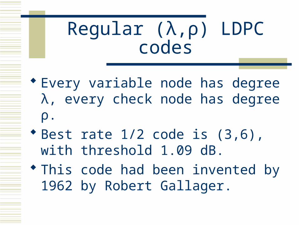
Regular (λ,ρ) LDPC codes

Every variable node has degree λ, every check node has degree ρ.

Best rate 1/2 code is (3,6), with threshold 1.09 dB.

This code had been invented by 1962 by Robert Gallager.

D.E. Simulation of (3,6) codes

Set SNR to 1.12 dB (.03 above threshold)

Watch fraction of "erroneous messages" from check to variable.

(note that this fraction does not characterize the distribution fully)

Improvement vs. current error fraction for Regular (3,6)

Improvement per iteration is plotted against current error fraction.

Note there is a single bottleneck which took most of the decoding iterations.

Irregular (λ, ρ) LDPC codes

a fraction λi of variable nodes have degree i. ρi of check nodes have degree i.

Edges are connected by a single random permutation.

Nodes have become specialized.

. . . . .

.

Variable nodes

Check nodes

πλ3

λn

ρ4

λ2

ρm

D.E. Simulation of Irregular Codes (Maximum degree 10)

Set SNR to 0.42 dB (~.03 above threshold)

Watch fraction of erroneous check to variable messages.

This Code was designed by Richardson et. al.

Comparison of Regular and Irregular codes

Notice that the Irregular graph is much flatter.

Note: Capacity achieving LDPC codes for the erasure channel were designed by making this line exactly flat.

Multi-edge-type construction

Edges of a particular "color" are connected through a permutation.

Edges become specialized. Each edge type has a different message distribution each iteration.

D.E. of MET codes.

For Multi-edge-type codes, Density evolution tracks the density of each type of message separately.

Comparison was made to real decoding, next slide (courtesy of Ken Andrews).

MET D.E. vs. decoder simulation

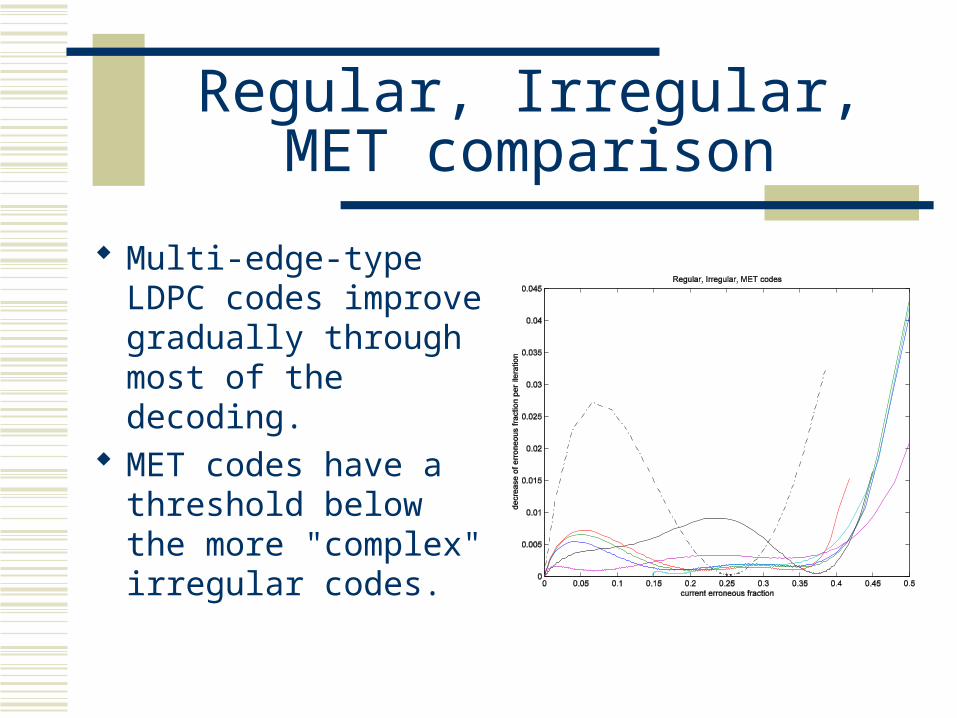
Regular, Irregular, MET comparison

Multi-edge-type LDPC codes improve gradually through most of the decoding.

MET codes have a threshold below the more "complex" irregular codes.

Design of Codes using D.E.

Density evolution provides a moderately fast way to evaluate single- and multi- edge type degree distributions (hypothesis-testing).

Much faster approximations to Density Evolution can easily be put into an outer loop which performs function minimization.

Semi-Analytic techniques exist as well.

Review

Iterative Message Passing can be used to decode LDPC codes.

Density Evolution can be used to predict the performance of MP for infinitely large codes.

More sophisticated classes of codes can be designed to close the gap to the Shannon limit.

Beyond MET Codes (future work)

Traditional LDPC codes are designed in two stages: design of the degree distribution and design of the specific graph.

Using very fast and accurate approximations to density evolution, we can evaluate the effect of placing or removing a single edge in the graph.

Using an evolutionary algorithm like Simulated Annealing, we can optimize the graph directly, changing the degree profile as needed.