THE ROLE OF QUANTITATIVE SEISMOLOGY

IN REAL-TIME AND DEFERRED

TSUNAMI STUDIES

Emile A. OKAL

Department of Earth & Planetary SceincesNorthwestern UniversityEvanston, IL 60208, USA

emile@earth.northwestern.edu

IRIS MetaDataWorkshop

Foz do Iguacu, Brasil

Segunda-Feira, 16 de Agosto 2.010

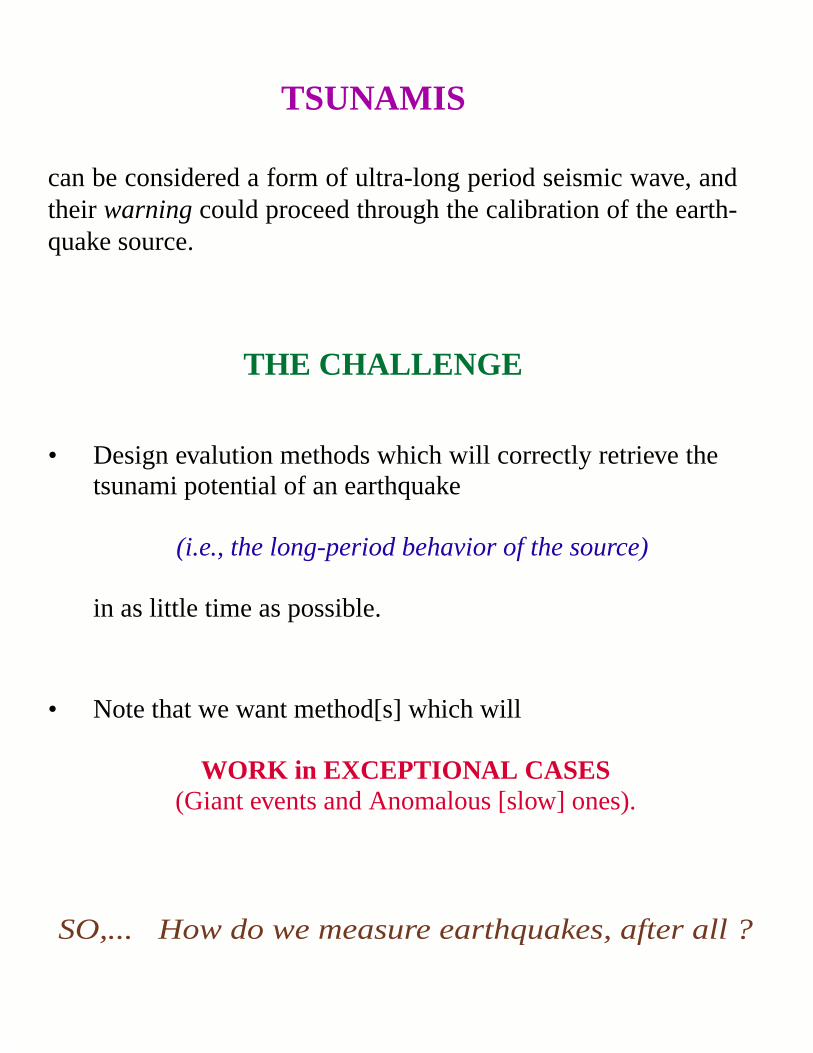
THE CHALLENGE

• Design evalution methods which will correctly retrieve thetsunami potential of an earthquake

(i.e., the long-period behavior of the source)

in as little time as possible.

• Note that we want method[s] which will

WORK in EXCEPTIONAL CASES(Giant events and Anomalous [slow] ones).

TSUNAMIS

can be considered a form of ultra-long period seismic wav e, andtheir warningcould proceed through the calibration of the earth-quake source.

SO,... Howdo we measure earthquakes, after all ?

THE FOUNDING FATHERS

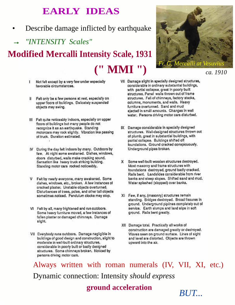
EARLY I DEAS

• Describe damage inflicted by earthquake

→→ "INTENSITY Scales"

Always written with roman numerals (IV, VII, XI, etc.) Dynamic connection: Intensityshould express

ground accelerationBUT...

Modified Mer calli Intensity Scale, 1931

(" MMI ")Fr. G. Mercalli at Vesuvius

ca. 1910

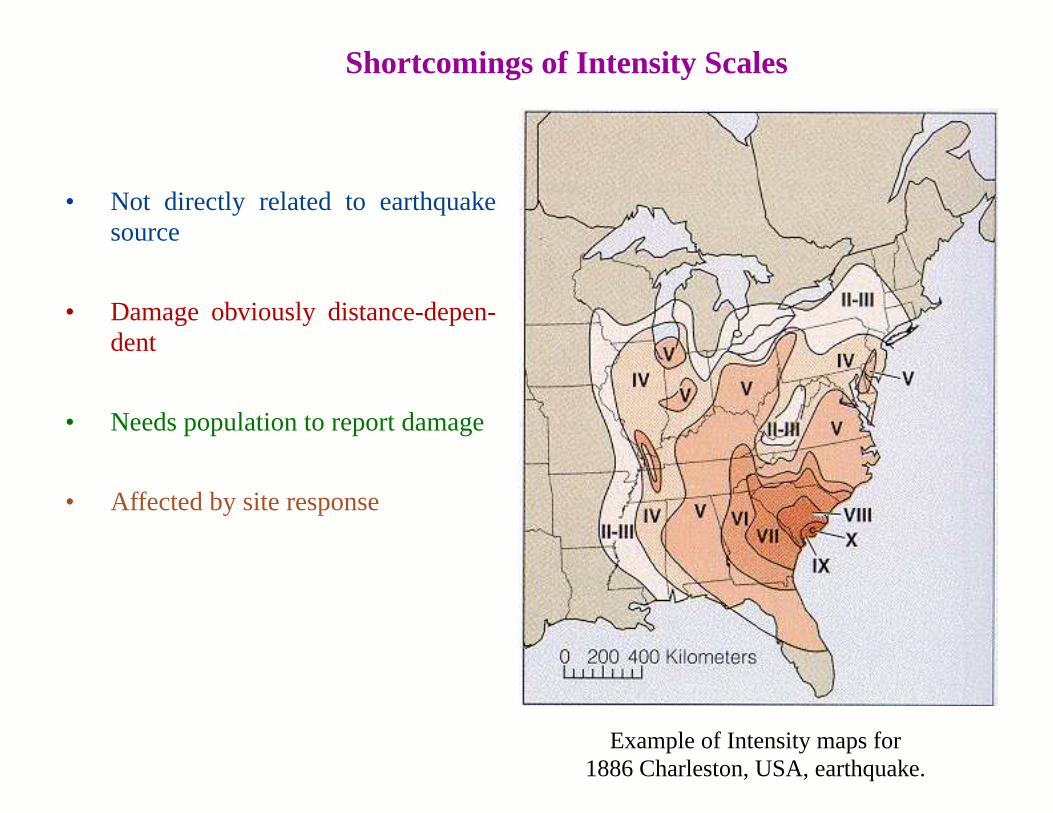
Shortcomings of Intensity Scales

• Not directly related to earthquakesource

• Damage obviously distance-depen-dent

• Needs population to report damage

• Affected by site response

Example of Intensity maps for1886 Charleston, USA, earthquake.

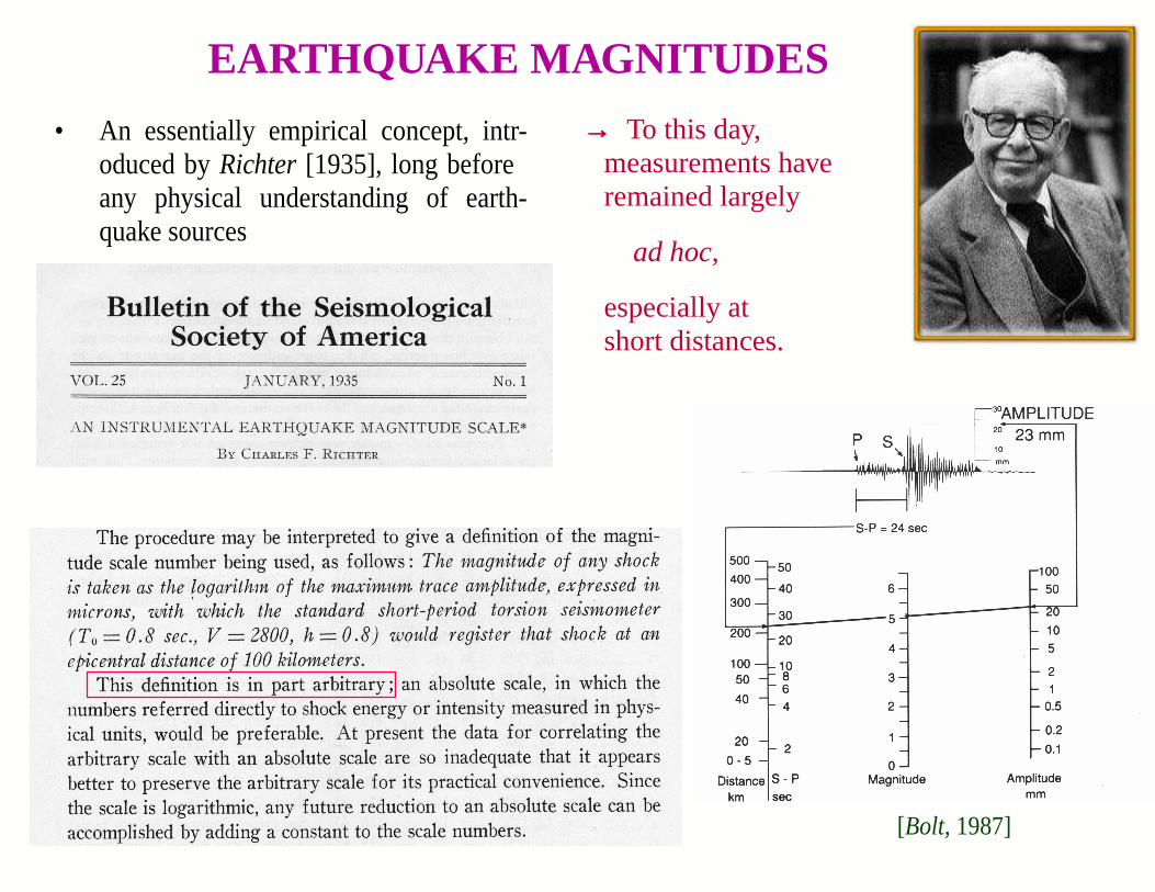
EARTHQ UAKE MAGNITUDES

• An essentially empirical concept, intr-oduced byRichter [1935], long beforeany physical understanding of earth-quake sources

• To this day, measurements haveremained largely ad hoc, especially atshort distances.

[Bolt, 1987]

→→ To this day,measurements haveremained largely

ad hoc,

especially atshort distances.

PROGRESS in the 1940s

• Apply worldwide

• Try (!!) to justify theoretically

→→ Leads to first worldwide quantifiedcatalogue of earthquakes

"Seismicity of the Earth"

Gutenberg and Richter[1944; 1954]

B. Gutenberg, 1958

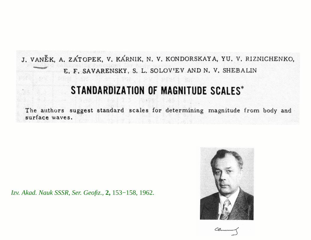
Izv. Akad. Nauk SSSR, Ser. Geofiz.,2, 153−158, 1962.

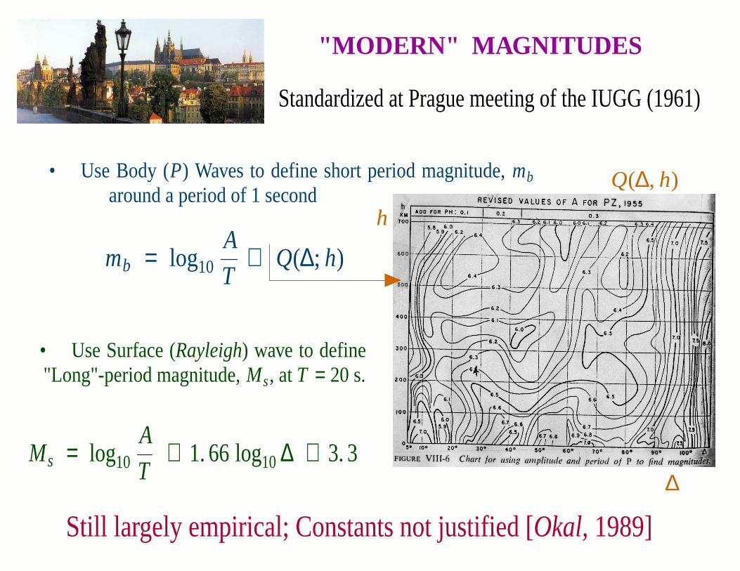
"MODERN" MA GNITUDES

Standardized at Prague meeting of the IUGG (1961)

• Use Body (P) Wav es to define short period magnitude,mbaround a period of 1 second

mb = log10A

T+ Q(∆; h)

• Use Surface (Rayleigh) wav eto define "Long"-period magnitude,Ms, at T = 20 s.

Ms = log10A

T+ 1. 66log10 ∆ + 3. 3

Still largely empirical; Constants not justified [Okal,1989]

∆

h

Q(∆, h)

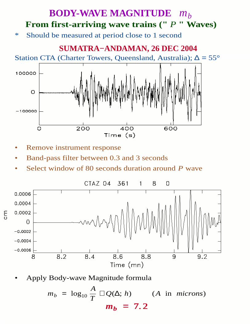
BODY-WAVE MAGNITUDE mbFrom first-arriving wa ve trains (" P " W av es)

* Should be measured at period close to 1 second

Station CTA (Charter Towers, Queensland, Australia);∆ = 55°

• Remove instrument response

• Band-pass filter between 0.3 and 3 seconds

• Select window of 80 seconds duration aroundP wave

• Apply Body-wav eMagnitude formula

mb = log10A

T+ Q(∆; h) (A in microns)

mb = 7. 2mb = 7. 2

SUMATRA−ANDAMAN, 26 DEC 2004

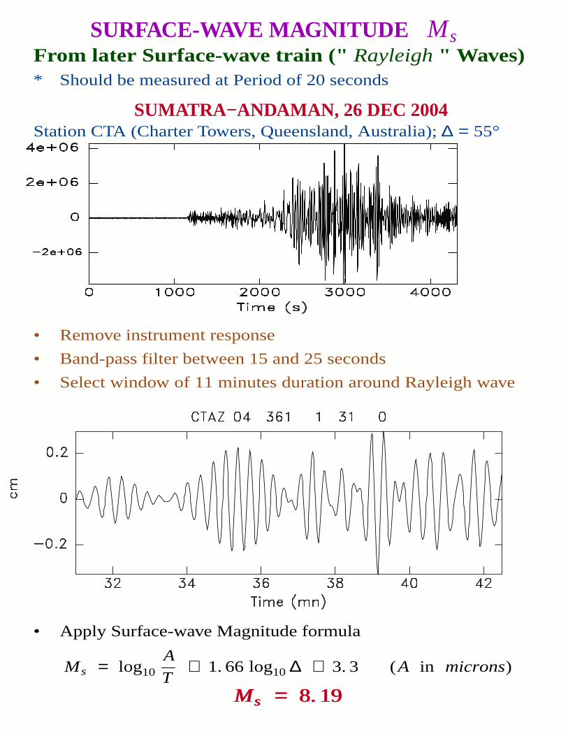
SURFACE-WAVE MAGNITUDE MsFrom later Surface-wave train (" Rayleigh" W av es)* Should be measured at Period of 20 seconds

Station CTA (Charter Towers, Queensland, Australia);∆ = 55°

• Remove instrument response

• Band-pass filter between 15 and 25 seconds

• Select window of 11 minutes duration around Rayleigh wav e

• Apply Surface-wav eMagnitude formula

Ms = log10A

T+ 1. 66log10 ∆ + 3. 3 (A in microns)

Ms = 8. 19Ms = 8. 19

SUMATRA−ANDAMAN, 26 DEC 2004

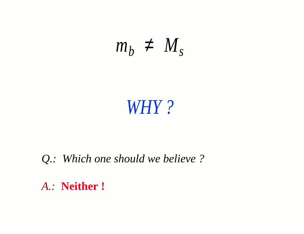
mb ≠ Ms

WHY ?

Q.: Which one should we believe ?

A.: Neither !

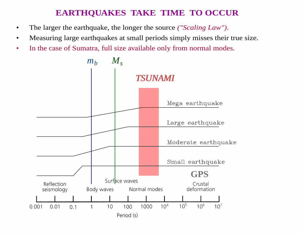
EARTHQ UAKES TAKE TIME T O OCCUR

• The larger the earthquake, the longer the source("Scaling Law").

• Measuring large earthquakes at small periods simply misses their true size.

• In the case of Sumatra, full size available only from normal modes.

mb Ms

TSUNAMITSUNAMI

GPS

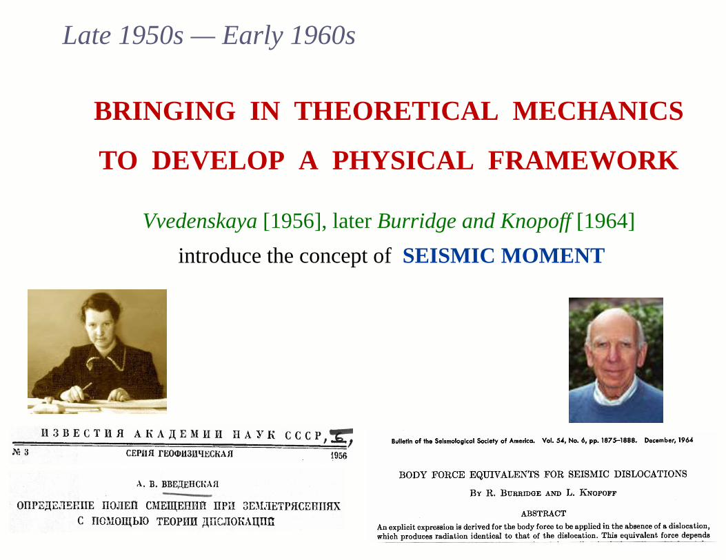
Late 1950s — Early 1960s

BRINGING IN THEORETICAL MECHANICS

TO DEVELOP A PHYSICAL FRAMEW ORK

Vvedenskaya[1956], laterBurridge and Knopoff[1964]

introduce the concept of SEISMIC MOMENT

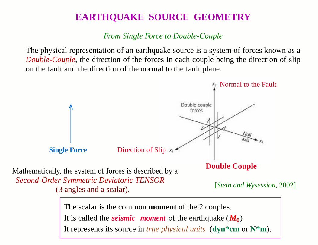
EARTHQ UAKE SOURCE GEOMETRY

Fr om Single Force to Double-Couple

The physical representation of an earthquake source is a system of forces known as aDouble-Couple, the direction of the forces in each couple being the direction of slipon the fault and the direction of the normal to the fault plane.

Mathematically, the system of forces is described by aSecond-Order Symmetric Deviatoric TENSOR

(3 angles and a scalar).

Single Force

Double Couple

Direction of Slip

Normal to the Fault

[Stein and Wysession,2002]

The scalar is the commonmomentof the 2 couples.It is called theseismic momentseismic momentof the earthquake (M0M0)It represents its source intrue physical units(dyn*cm or N*m ).

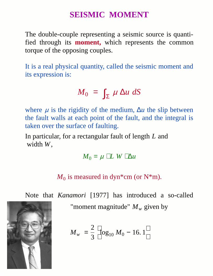
SEISMIC MOMENT

The double-couple representing a seismic source is quanti-fied through itsmoment, which represents the commontorque of the opposing couples.

It is a real physical quantity, called the seismic moment andits expression is:

M0 = ∫Σ µ ∆u dS

whereµ is the rigidity of the medium,∆u the slip betweenthe fault walls at each point of the fault, and the integral istaken over the surface of faulting.

In particular, for a rectangular fault of lengthL andwidth W,

M0 = µ ⋅ L W ⋅ ∆u

M0 is measured in dyn*cm (or N*m).

Note that Kanamori [1977] has introduced a so-called

"moment magnitude"Mw given by

Mw =2

3log10 M0 − 16. 1

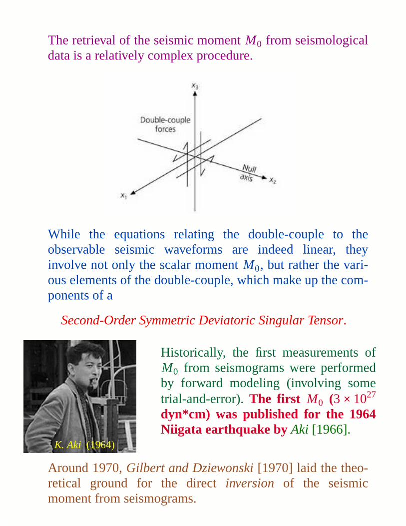
The retrieval of the seismic momentM0 from seismologicaldata is a relatively complex procedure.

While the equations relating the double-couple to theobservable seismic wav eforms are indeed linear, theyinvolve not only the scalar momentM0, but rather the vari-ous elements of the double-couple, which make up the com-ponents of a

Second-Order Symmetric Deviatoric Singular Tensor.

Historically, the first measurements ofM0 from seismograms were performedby forward modeling (involving sometrial-and-error).The first M0 (3 × 1027

dyn*cm) was published for the 1964Niigata earthquake by Aki [1966].

Around 1970,Gilbert and Dziewonski[1970] laid the theo-retical ground for the directinversion of the seismicmoment from seismograms.

K. Aki (1964)

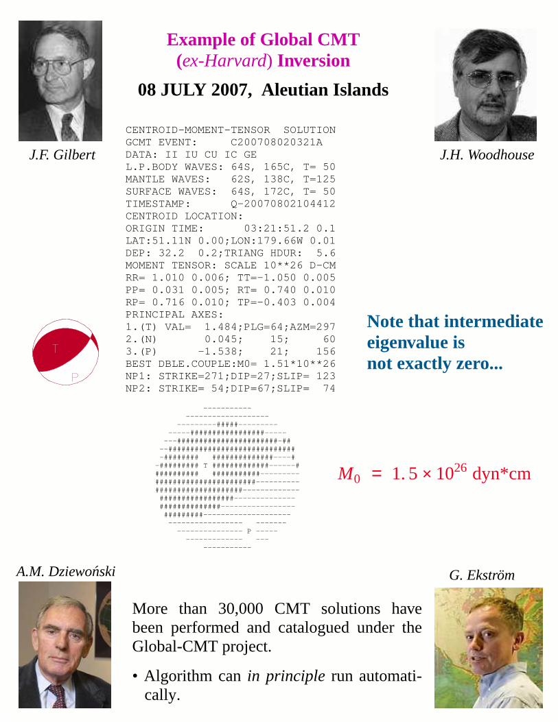
CENTROID-MOMENT-TENSOR SOLUTIONGCMT EVENT: C200708020321A DATA: II IU CU IC GE L.P.BODY WAVES: 64S, 165C, T= 50MANTLE WAVES: 62S, 138C, T=125SURFACE WAVES: 64S, 172C, T= 50TIMESTAMP: Q-20070802104412CENTROID LOCATION:ORIGIN TIME: 03:21:51.2 0.1LAT:51.11N 0.00;LON:179.66W 0.01DEP: 32.2 0.2;TRIANG HDUR: 5.6MOMENT TENSOR: SCALE 10**26 D-CMRR= 1.010 0.006; TT=-1.050 0.005PP= 0.031 0.005; RT= 0.740 0.010RP= 0.716 0.010; TP=-0.403 0.004PRINCIPAL AXES:1.(T) VAL= 1.484;PLG=64;AZM=2972.(N) 0.045; 15; 603.(P) -1.538; 21; 156BEST DBLE.COUPLE:M0= 1.51*10**26NP1: STRIKE=271;DIP=27;SLIP= 123NP2: STRIKE= 54;DIP=67;SLIP= 74

----------- ------------------- ---------#####--------- -----#################----- ---#######################-## --############################# -######## ##############----# -######### T #############------# ########## ###########--------- #######################---------- ####################------------- #################-------------- ##############----------------- #########-------------------- ----------------- ------- --------------- P ----- ------------- --- -----------

Example of Global CMT(ex-Harvard) Inversion

More than 30,000 CMT solutions havebeen performed and catalogued under theGlobal-CMT project.

• Algorithm canin principle run automati-cally.

08 JULY 2007, AleutianIslands

Note that intermediateeigenvalue isnot exactly zero...

M0 = 1. 5× 1026 dyn*cm

J.F. Gilbert

A.M. Dziewon´ski

J.H. Woodhouse

G. Ekstro m

TSUNAMI WARNING: THE CHALLENGE

• Upon detection of a teleseismic earthquake, assess in real-timeits tsunami potential.

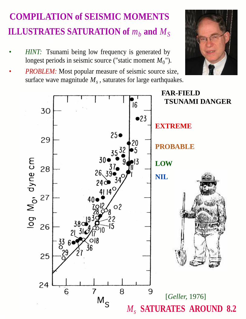
• HINT: Tsunami being low frequency is generated by longest periods in seismic source ("static momentM0").

• PROBLEM:Most popular measure of seismic source size, surface wav emagnitudeMs , saturates for large earthquakes.

EXTREME

PROBABLE

LOW

NIL

FAR-FIELDTSUNAMI DANGER

[Geller,1976]

Ms SATURATES AROUND 8.2

COMPILATION of SEISMIC MOMENTS

ILLUSTRATES SATURATION of mb and MS

CMT AND ITS LIMIT ATIONS

→ CMT inversions are now performed in quasi-real time

→ But this approach still suffers from limitations:

• Needs a large database (tens of stations)

• Automated algorithm is ,per force, hard-wired,i.e., universal.

• It will need to be [manually] adapted to recognize anomalous events, either gigantic (e.g., Sumatra) or slow ("tsunami earthquakes"; stay tuned).

• There remains the quest for ultra-long periods to properly assess tsunami potential.

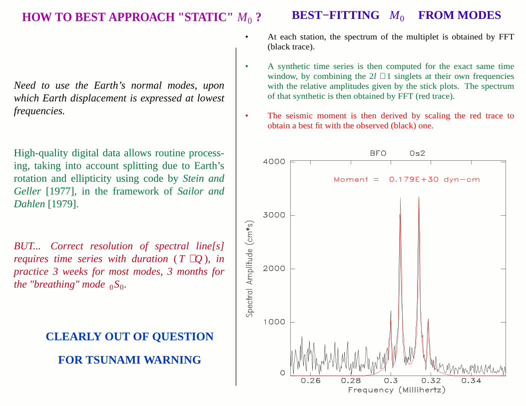
BEST−FITTING M0

• At each station, the spectrum of the multiplet is obtained by FFT(black trace).

• A synthetic time series is then computed for the exact same timewindow, by combining the 2l + 1 singlets at their own frequencieswith the relative amplitudes given by the stick plots. The spectrumof that synthetic is then obtained by FFT (red trace).

• The seismic moment is then derived by scaling the red trace toobtain a best fit with the observed (black) one.

HOW TO BEST APPROACH "STATIC" M0 ? FROM MODES

Need to use the Earth’s normal modes, uponwhich Earth displacement is expressed at lowestfrequencies.

High-quality digital data allows routine process-ing, taking into account splitting due to Earth’srotation and ellipticity using code byStein andGeller [1977], in the framework of Sailor andDahlen[1979].

BUT... Correct resolution of spectral line[s]requires time series with duration ( T ⋅ Q ), inpractice 3 weeks for most modes, 3 months forthe "breathing" mode0S0.

CLEARL Y OUT OF QUESTION

FOR TSUNAMI WARNING

TIMELINE OF MOMENT DETERMIN ATIONS

SUMATRA 2004

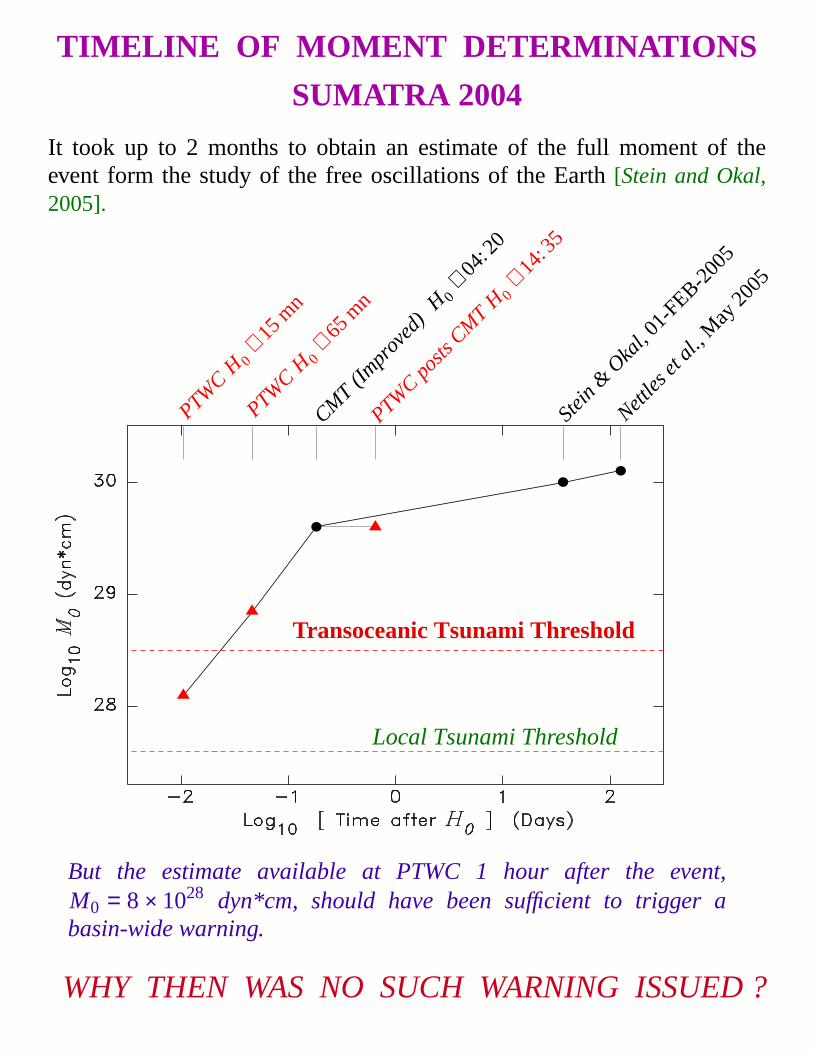
It took up to 2 months to obtain an estimate of the full moment of theev ent form the study of the free oscillations of the Earth[Stein and Okal,2005].

But the estimate available at PTWC 1 hour after the event,M0 = 8 × 1028 dyn*cm, should have been sufficient to trigger abasin-wide warning.

WHY THEN WAS NO SUCH WARNING ISSUED?

Local Tsunami Threshold

Tr ansoceanic Tsunami Threshold

PTWC H0

+ 15 m

n

PTWC H0

+ 65 m

n

CMT (I

mpr

oved

) H0

+ 04: 2

0

PTWC p

osts C

MT

H0+ 14

: 35

Stein &

Oka

l,01-

FEB-200

5

Nettle

s et

al.,M

ay 2

005

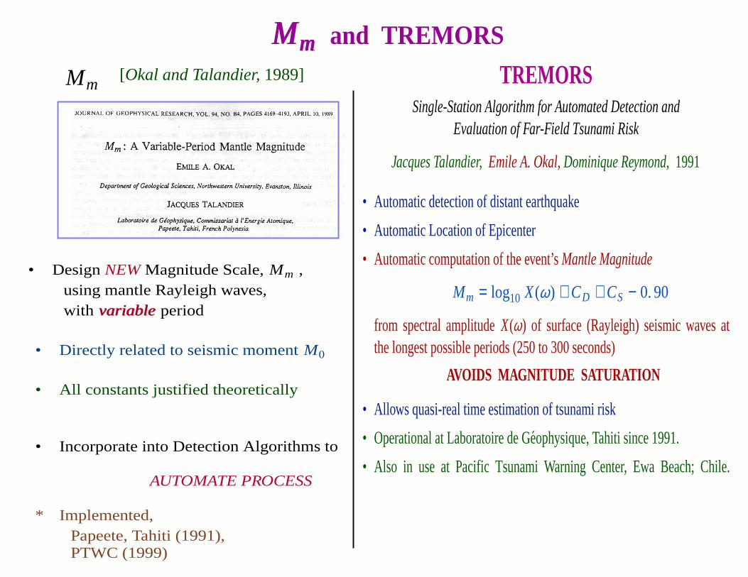
MmMm and TREMORS[Okal and Talandier,1989]

• DesignNEWMagnitude Scale,Mm ,using mantle Rayleigh wav es,with variablevariableperiod

• Directly related to seismic momentM0

• All constants justified theoretically

• Incorporate into Detection Algorithms to

AUTOMATE PROCESS

* I mplemented,Papeete, Tahiti (1991),PTWC (1999)

TREMORSSingle-Station Algorithm for Automated Detection and

Evaluation of Far-Field Tsunami Risk

Jacques Talandier, Emile A. Okal, Dominique Reymond,1991

• Automatic detection of distant earthquake

• Automatic Location of Epicenter

• Automatic computation of the event’s Mantle Magnitude

Mm = log10 X(ω) + CD + CS − 0. 90

from spectral amplitudeX(ω) of surface (Rayleigh) seismic wav es atthe longest possible periods (250 to 300 seconds)

AV OIDS MAGNITUDE SATURATION

• Allows quasi-real time estimation of tsunami risk

• Operational at Laboratoire de Ge´ophysique, Tahiti since 1991.

• Also in use at Pacific Tsunami Warning Center, Ewa Beach; Chile.

Mm

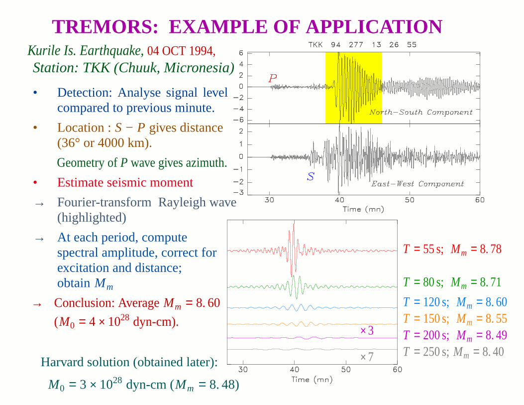
T = 55 s; Mm = 8. 78

T = 80 s; Mm = 8. 71

T = 120 s; Mm = 8. 60T = 150 s; Mm = 8. 55T = 200 s; Mm = 8. 49× 3

T = 250 s;Mm = 8. 40× 7

TREMORS: EXAMPLE OF APPLICATIONKurile Is. Earthquake,04 OCT 1994,Station: TKK (Chuuk, Micronesia)

• Detection: Analyse signal levelcompared to previous minute.

• Location :S − P gives distance(36° or 4000 km).

Geometry ofP wave giv es azimuth.

• Estimate seismic moment

→ Fourier-transform Rayleighwave(highlighted)

→ At each period, computespectral amplitude, correct forexcitation and distance;obtainMm

→ Conclusion: AverageMm = 8. 60

(M0 = 4 × 1028 dyn-cm).

Harvard solution (obtained later):

M0 = 3 × 1028 dyn-cm (Mm = 8. 48)

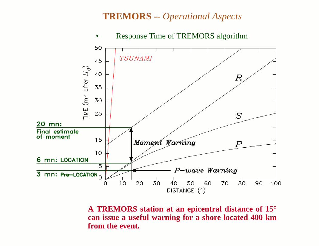
TREMORS -- Operational Aspects

• Response Time of TREMORS algorithm

A TREMORS station at an epicentral distance of 15°can issue a useful warning for a shore located 400 kmfrom the event.

MMm CAN WORK at SHORT DISTANCES

Tested by Okal and Talandier [1992] down to

∆ = 1. 5° (165 km).

MMm WORKS for GIGANTIC EVENTS

Chile, 1960

Works even on sev erely clipped records obtained on instru-ments with poor dynamic.

[Okal and Talandier,1991]

MMm CAN WORK for HISTORICAL EVENTS

Important for reassessment of old events, based onvery sparse datasets.

17 AUGUST 1906 -- Aleutian Islands

Wiechert mechanical seismometer, Strasbourg

Mm = 8. 58; M0 = 3. 8× 1028 dyn*cm

Mm: APPLICABLE in CHALLENGING CONTEXTS

→ In a series of targetted studies, wehave shown that theMm algorithmcan work successfully in challengingcontexts, thereby illustrating its relia-bility and robustness.

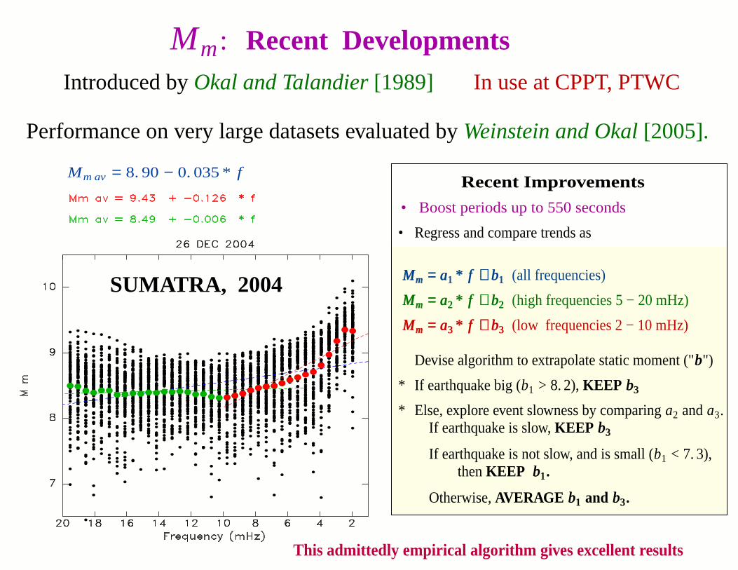
Mm: Recent DevelopmentsIntroduced byOkal and Talandier[1989]

Performance on very large datasets evaluated byWeinstein and Okal[2005].

In use at CPPT, PTWC

Recent Improvements

• Boost periods up to 550 seconds

• Regress and compare trends as

Mm = a1 * f + b1Mm = a1 * f + b1 (all frequencies)

Mm = a2 * f + b2Mm = a2 * f + b2 (high frequencies 5 − 20 mHz)

Mm = a3 * f + b3Mm = a3 * f + b3 (low frequencies 2 − 10 mHz)

Devise algorithm to extrapolate static moment ("bb")

* I f earthquake big (b1 > 8. 2), KEEP b3b3

* Else, explore event slowness by comparinga2 anda3.If earthquake is slow, KEEP b3b3

If earthquake is not slow, and is small (b1 < 7. 3),thenKEEP b1b1.

Otherwise,AVERAGE b1b1 and b3b3.

This admittedly empirical algorithm gives excellent results

Mm av = 8. 90− 0. 035 * f

SUMATRA, 2004

RETRIEVING DIVERSITY IN SEISMIC SOURCES

Not All Earthquakes Are Created Equal...

or

IDENTIFYING THE SCOFFLA WS

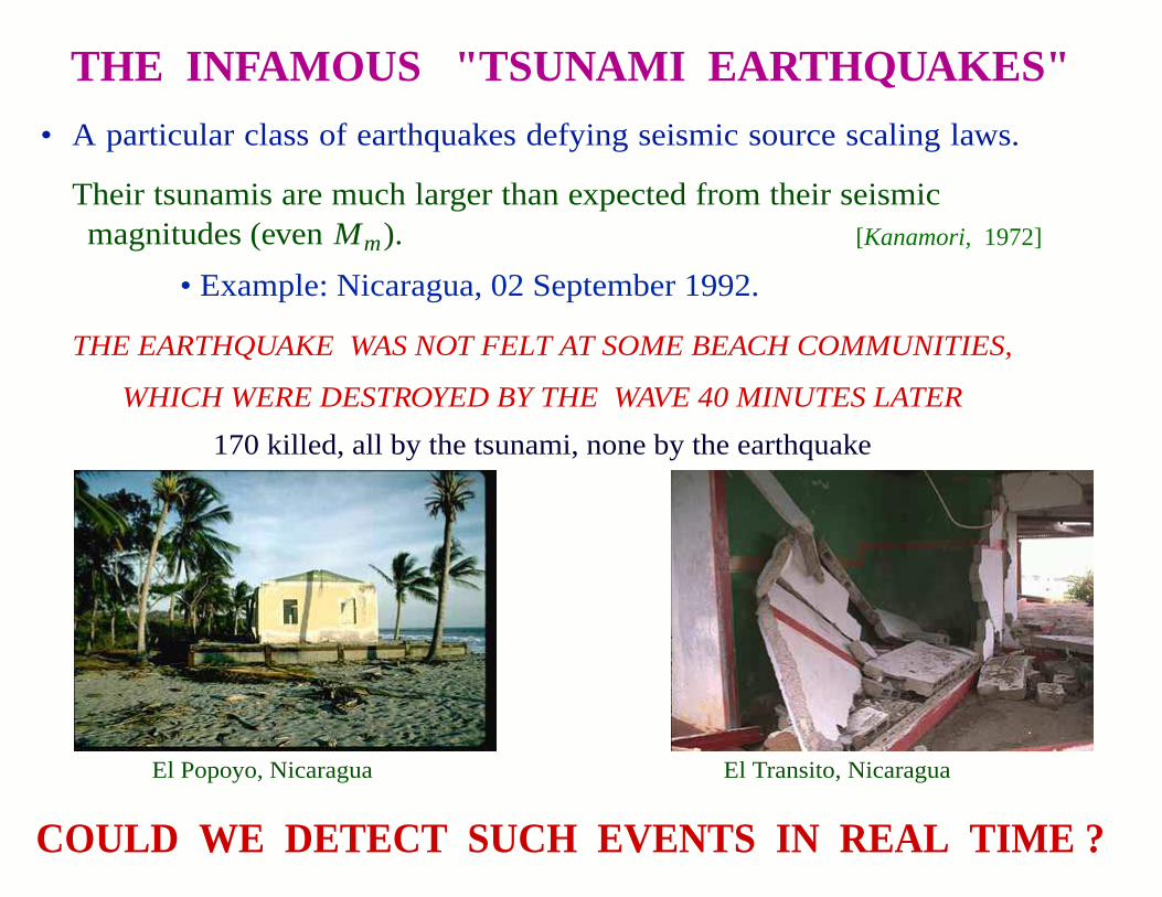
THE INFAMOUS "TSUN AMI EAR THQUAKES"

• A particular class of earthquakes defying seismic source scaling laws.

Their tsunamis are much larger than expected from their seismicmagnitudes (even Mm).

• Example: Nicaragua, 02 September 1992.

THE EARTHQUAKE WAS NOT FELT AT SOME BEACH COMMUNITIES,

WHICH WERE DESTROYED BY THEWAVE 40 MINUTES LATER

170 killed, all by the tsunami, none by the earthquake

El Transito, NicaraguaEl Popoyo, Nicaragua

COULD WE DETECT SUCH EVENTS IN REAL TIME ?

[Kanamori, 1972]

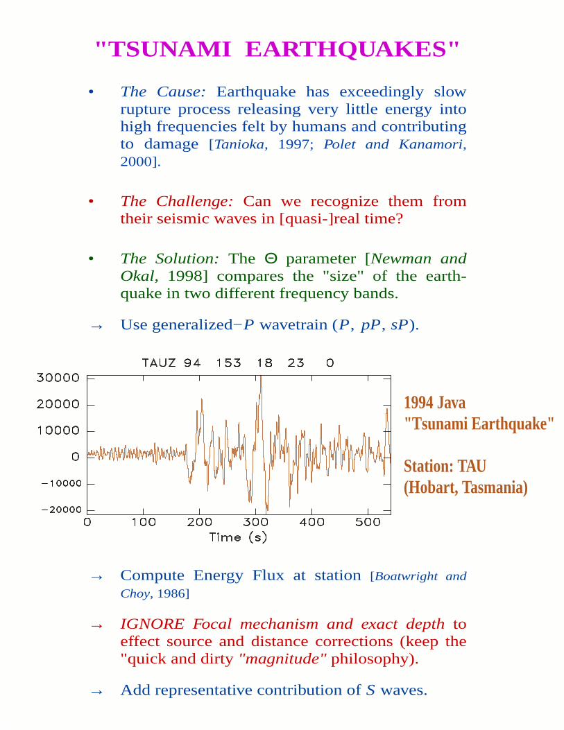
"TSUNAMI EAR THQUAKES"

• The Cause:Earthquake has exceedingly slowrupture process releasing very little energy intohigh frequencies felt by humans and contributingto damage[Tanioka, 1997; Polet and Kanamori,2000].

• The Challenge: Can we recognize them fromtheir seismic wav es in [quasi-]real time?

• The Solution:The Θ parameter [Newman andOkal, 1998] compares the "size" of the earth-quake in two different frequency bands.

→ Use generalized−P wavetrain (P, pP, sP).

→ Compute Energy Flux at station[Boatwright and

Choy, 1986]

→ IGNORE Focal mechanism and exact depthtoeffect source and distance corrections (keep the"quick and dirty"magnitude"philosophy).

→ Add representative contribution ofS waves.

1994 Jav a"Tsunami Earthquake"

Station: TAU(Hobart, Tasmania)

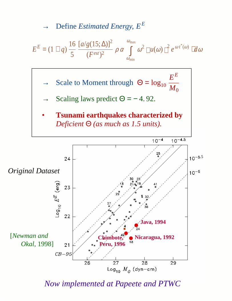
→ DefineEstimated Energy, EE

EE = (1 + q)16

5

[a/g(15;∆)]2

(Fest)2ρ α

ωmax

ωmin

∫ ω2 u(ω) 2 eω t* (ω) ⋅ dω

→ Scale to Moment throughΘ = log10EE

M0

→ Scaling laws predictΘ = −4. 92.

• Tsunami earthquakes characterized byDeficientΘ (as much as 1.5 units).

Now implemented at Papeete and PTWC

••• Nicaragua, 1992

Java, 1994

Chimbote,Peru, 1996

.5

Original Dataset

[Newman andOkal,1998]

SPEEDING UP THE WARNING

Long−Period Waves are Typically [Slow] Surface Waves

This delaysthe process (we must wait for them 30 to 60 mn)

Can the faster Body Waves (mainly P) be used to retrieve

the Long-Period Characteristics of the Source ?

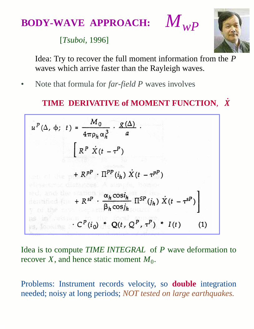
BODY-WAVE APPROACH:

[Tsuboi,1996]

Idea: Try to recover the full moment information from thePwaves which arrive faster than the Rayleigh wav es.

• Note that formula forfar-field P waves inv olves

TIME DERIV ATIVE of MOMENT FUNCTION , XX

Idea is to computeTIME INTEGRALof P wave deformation torecover X, and hence static momentM0.

Problems: Instrument records velocity, so double integrationneeded; noisy at long periods;NOT tested on large earthquakes.

MwP

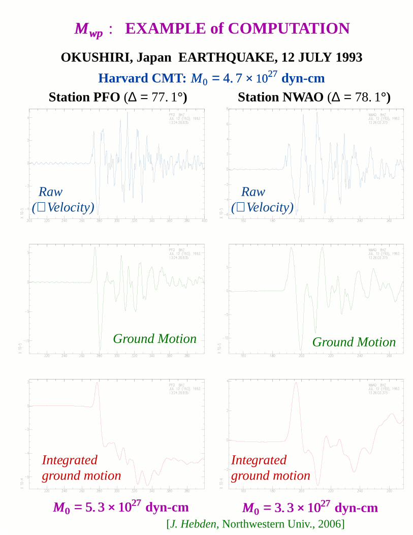
MwpMwp : EXAMPLE of COMPUT ATION

OKUSHIRI, J apan EARTHQUAKE, 12 JULY 1993

Harvard CMT: M0 = 4. 7× 1027M0 = 4. 7× 1027 dyn-cmStation PFO (∆ = 77. 1°) Station NWAO (∆ = 78. 1°)

Raw(∼ Velocity)

Raw(∼ Velocity)

Ground Motion Ground Motion

Integratedground motion

Integratedground motion

M0 = 5. 3× 1027M0 = 5. 3× 1027 dyn-cm M0 = 3. 3× 1027M0 = 3. 3× 1027 dyn-cm[J. Hebden,Northwestern Univ., 2006]

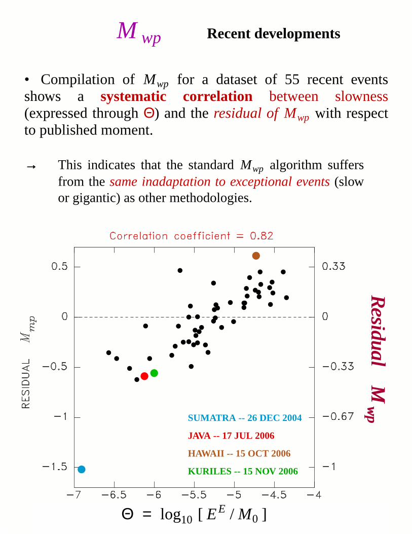
M wp Recent developments

• Compilation of Mwp for a dataset of 55 recent eventsshows a systematic correlation between slowness(expressed throughΘ) and theresidual of Mwp with respectto published moment.

Re

sidu

al

Mw

pR

esid

ua

l M

wp

→→ This indicates that the standardMwp algorithm suffersfrom thesame inadaptation to exceptional events(slowor gigantic) as other methodologies.

SUMATRA -- 26 DEC 2004

JAVA -- 17 JUL 2006

HAWAII -- 15 OCT 2006

KURILES -- 15 NOV 2006

Θ = log10 [ EE / M0 ]

M wp

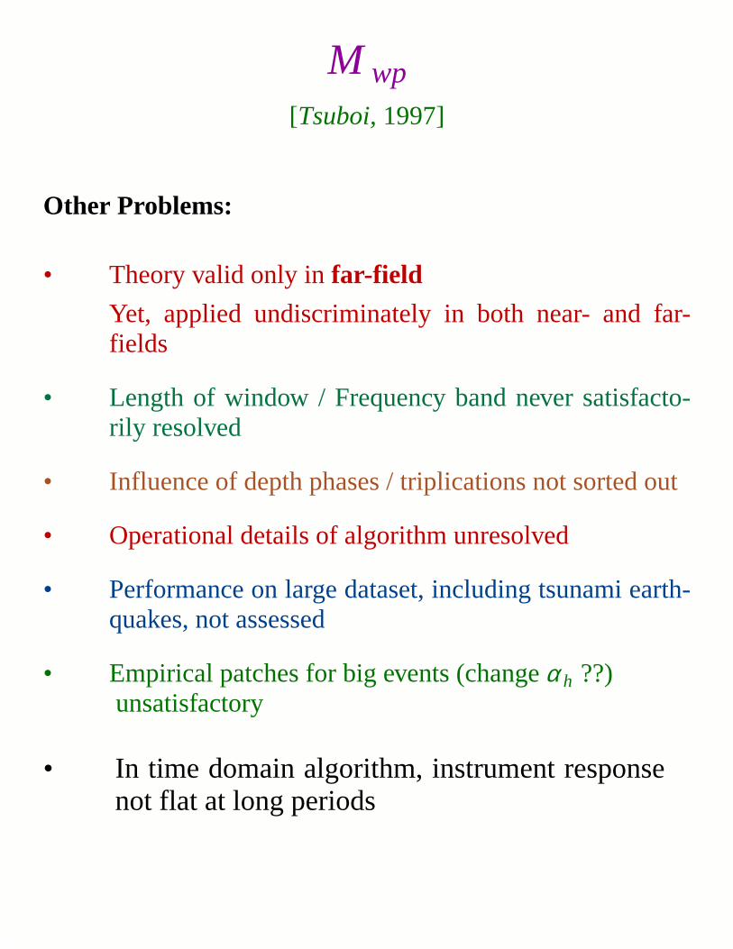
[Tsuboi,1997]

Other Problems:

• Theory valid only infar-field

Yet, applied undiscriminately in both near- and far-fields

• Length of window / Frequency band never satisfacto-rily resolved

• Influence of depth phases / triplications not sorted out

• Operational details of algorithm unresolved

• Performance on large dataset, including tsunami earth-quakes, not assessed

• Empirical patches for big events (changeα h ??)unsatisfactory

• In time domain algorithm, instrument responsenot flat at long periods

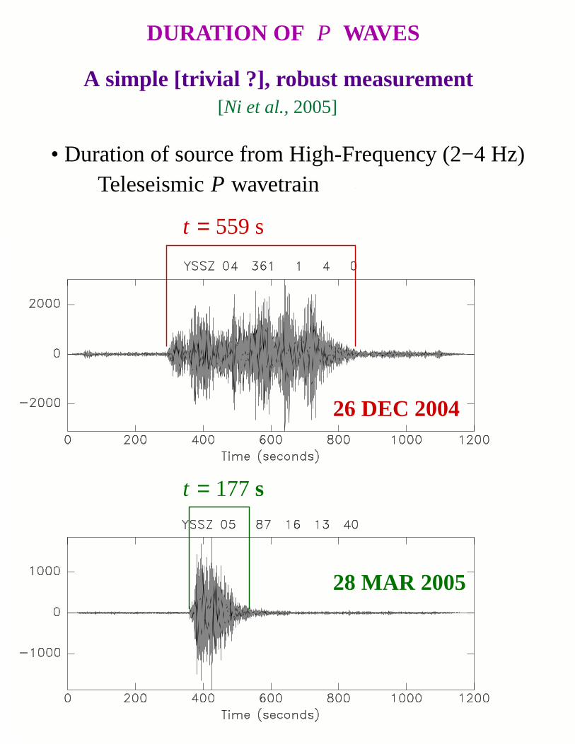
A simple [trivial ?], robust measurement[Ni et al.,2005]

• Duration of source from High-Frequency (2−4 Hz)TeleseismicP wavetrain

26 DEC 2004

t = 559 s

28 MAR 2005

t = 177s

DURATION OF P WAVES

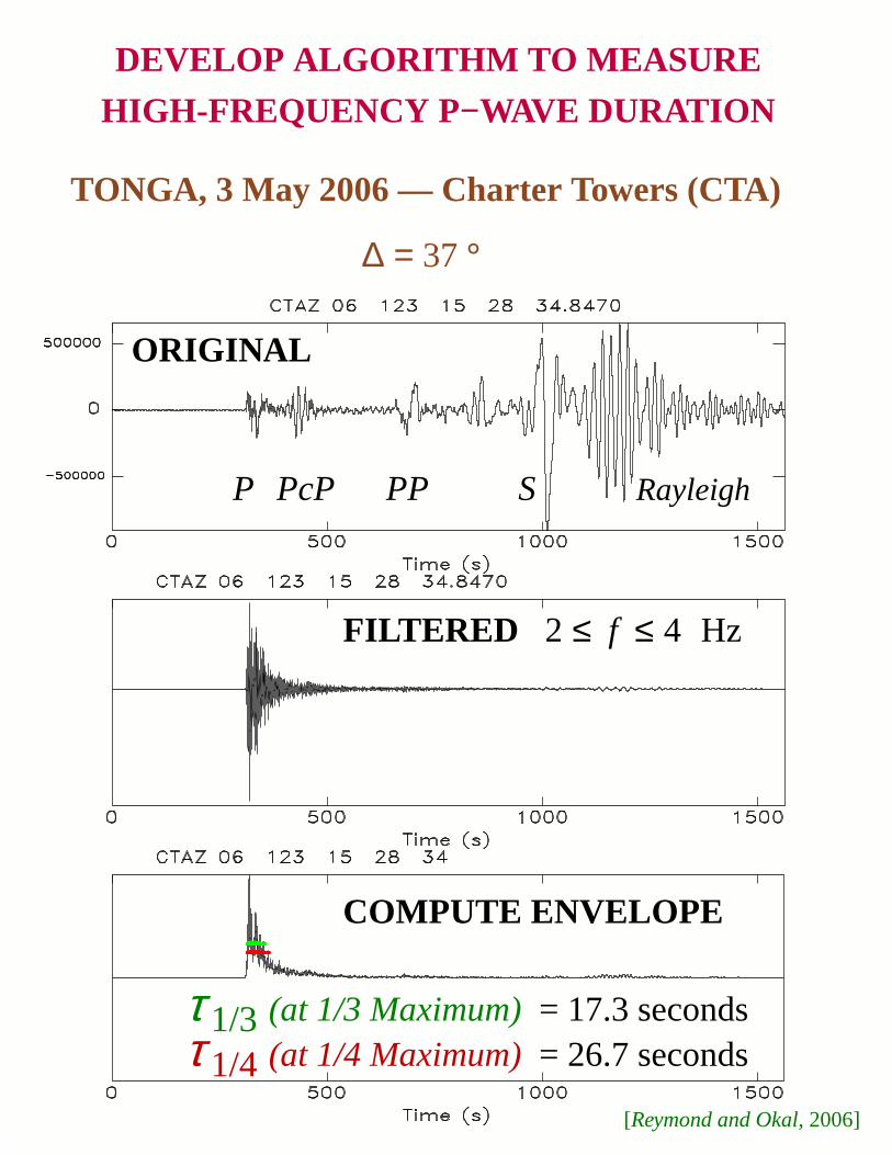
DEVELOP ALGORITHM T O MEASURE

HIGH-FREQUENCY P−WAVE DURATION

TONGA, 3 May 2006 — Charter Towers (CTA)

∆ = 37 °

P SPcP PP Rayleigh

ORIGINAL

FILTERED 2 ≤ f ≤ 4 Hz

COMPUTE ENVELOPE

τ 1/3 (at 1/3 Maximum)= 17.3 secondsτ 1/4 (at 1/4 Maximum)= 26.7 seconds

[Reymond and Okal,2006]

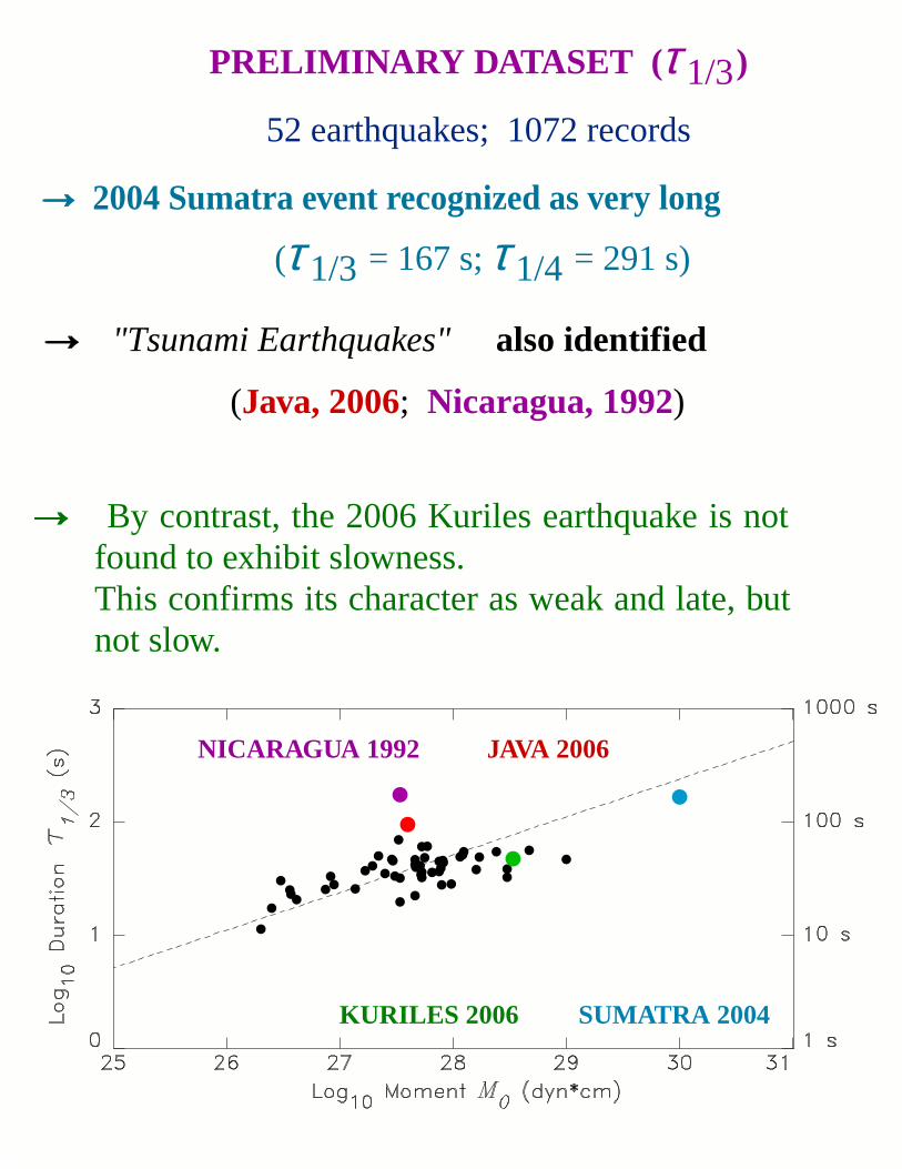
PRELIMINAR Y DAT ASET (τ 1/3)

52 earthquakes; 1072records

→→ 2004 Sumatra event recognized as very long

→→ "Tsunami Earthquakes" also identified

(τ 1/3 = 167 s;τ 1/4 = 291 s)

(Java, 2006; Nicaragua, 1992)

→→ By contrast, the 2006 Kuriles earthquake is notfound to exhibit slowness.This confirms its character as weak and late, butnot slow.

SUMATRA 2004

JAVA 2006NICARAGU A 1992

KURILES 2006

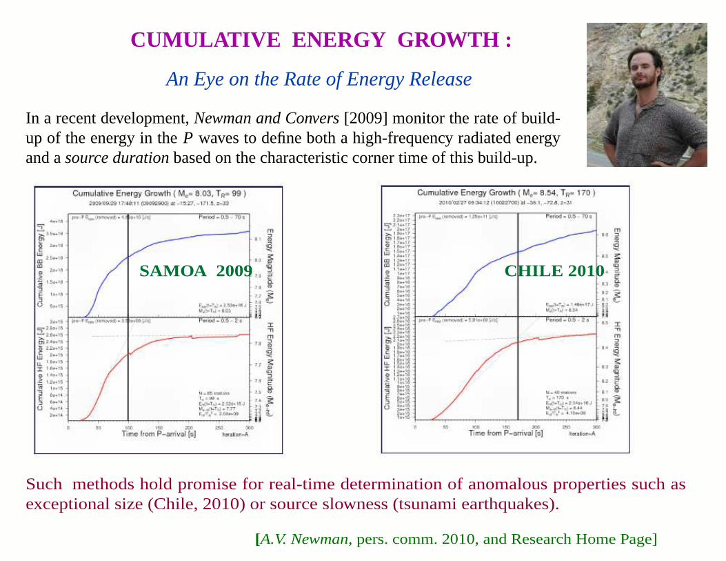
CUMULA TIVE ENERGY GR OWTH :

An Eye on the Rate of Energy Release

In a recent development,Newman and Convers[2009] monitor the rate of build-up of the energy in theP waves to define both a high-frequency radiated energyand asource durationbased on the characteristic corner time of this build-up.

Such methodshold promise for real-time determination of anomalous properties such asexceptional size (Chile, 2010) or source slowness (tsunami earthquakes).

SAMOA 2009 CHILE 2010

[A.V. Newman,pers. comm. 2010, and Research Home Page]

WW Phase

for "Whistling"

or perhaps "Wisdom"...

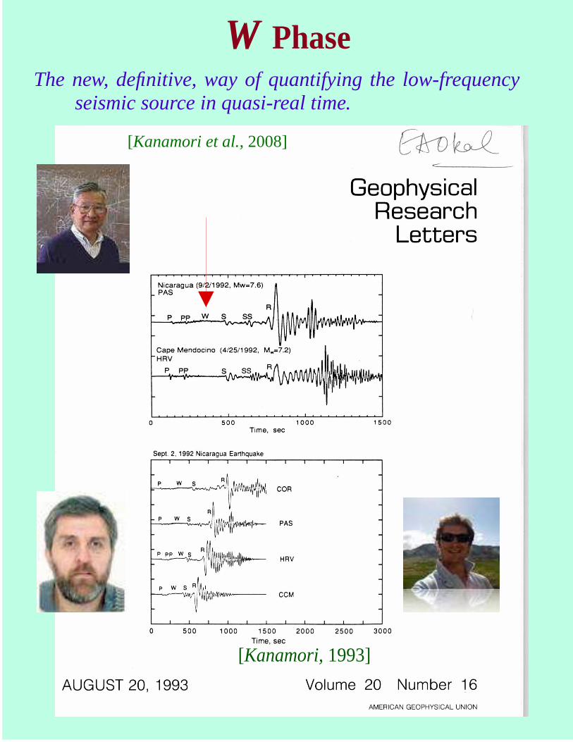
WWPhase

[Kanamori,1993]

The new, definitive, way of quantifying the low-frequencyseismic source in quasi-real time.

[Kanamori et al.,2008]

What IS the WW Phase ?

A combination of multiply-reflected body phases sam-pling the upper mantle at very low frequencies (1 to5 mHz) and arriving betweenP andRayleighwaves.

→ The multiply reverberated nature of this amalgamof PP, PPP, PPS, PSS, etc. is reminiscent of the"whistling" mode of radio transmission in theatmosphere, hence the nameWW phase coined byKanamori[1993].

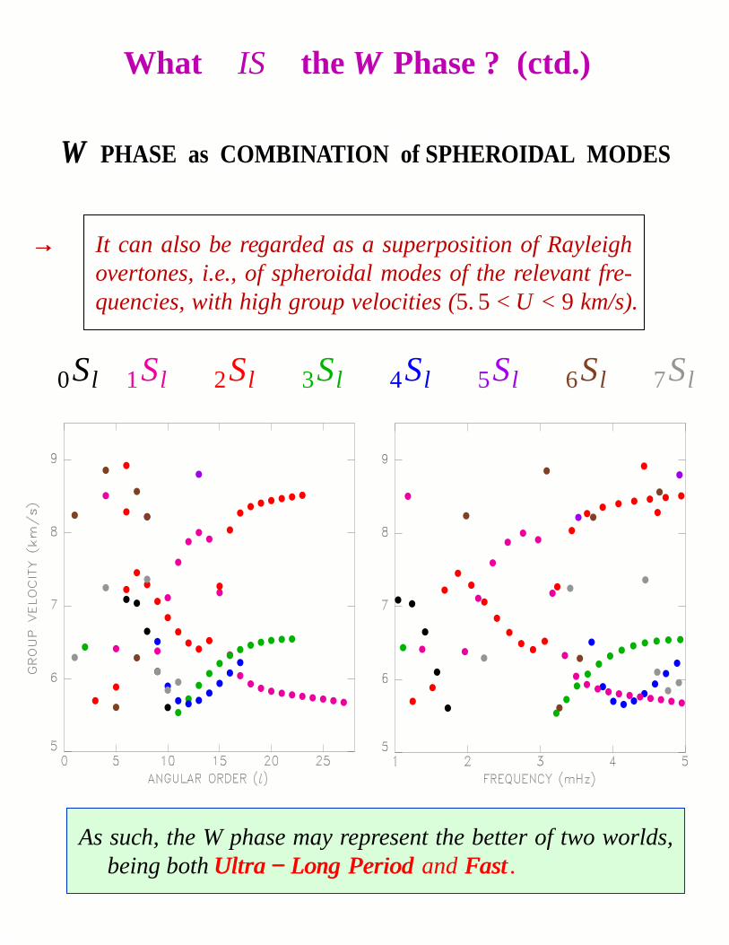
What IS the WW Phase ? (ctd.)

A combination of multiply-reflected body phases sam-pling the upper mantle at very low frequencies (1 to5 mHz) and arriving betweenP andRayleighwaves.

→→ It can also be regarded as a superposition of Rayleighovertones, i.e., of spheroidal modes of the relevant fre-quencies, with high group velocities (5. 5< U < 9 km/s).

0Sl 1Sl 2Sl 3Sl 4Sl 5Sl 6Sl 7Sl

WW PHASE as COMBINATION of SPHEROIDAL MODES

As such, the W phase may represent the better of two worlds,being bothUltra − Long PeriodUltra − Long Periodand FastFast.

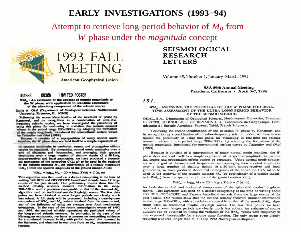
EARLY I NVESTIGATIONS (1993−94)

Attempt to retrieve long-period behavior ofM0 fromW phase under themagnitudeconcept

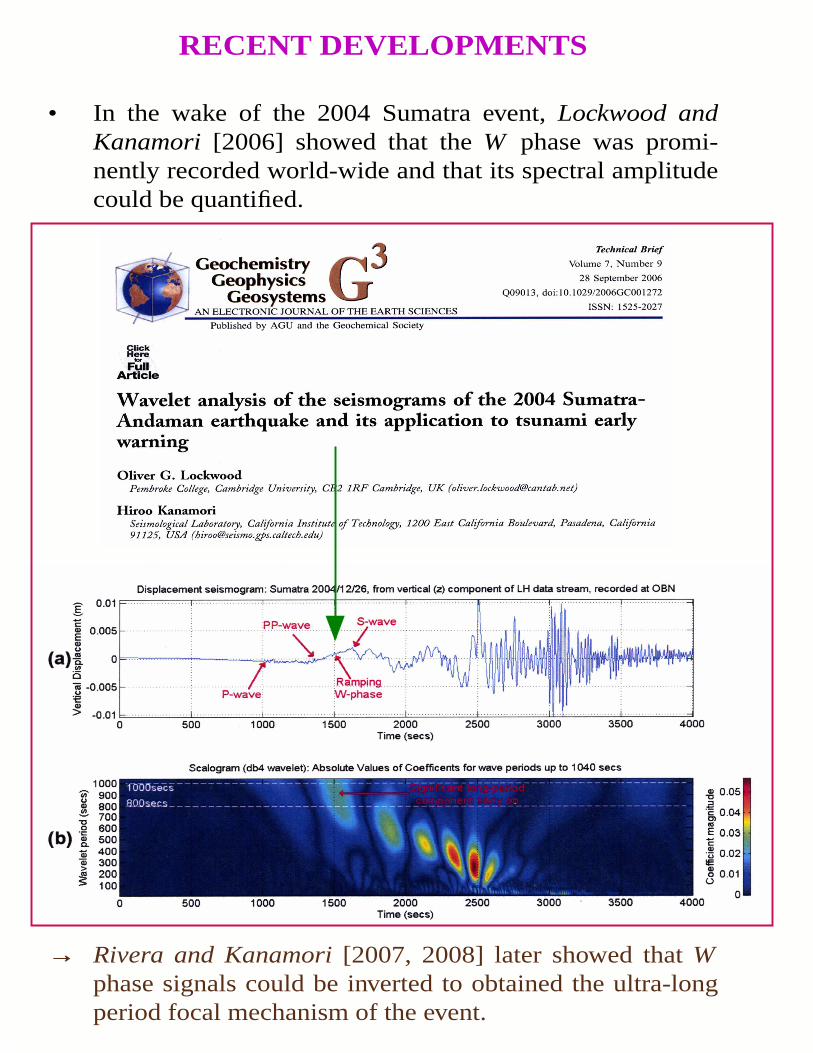
RECENT DEVELOPMENTS

• In the wake of the 2004 Sumatra event, Lockwood andKanamori [2006] showed that theW phase was promi-nently recorded world-wide and that its spectral amplitudecould be quantified.

→→ Rivera and Kanamori[2007, 2008] later showed thatWphase signals could be inverted to obtained the ultra-longperiod focal mechanism of the event.

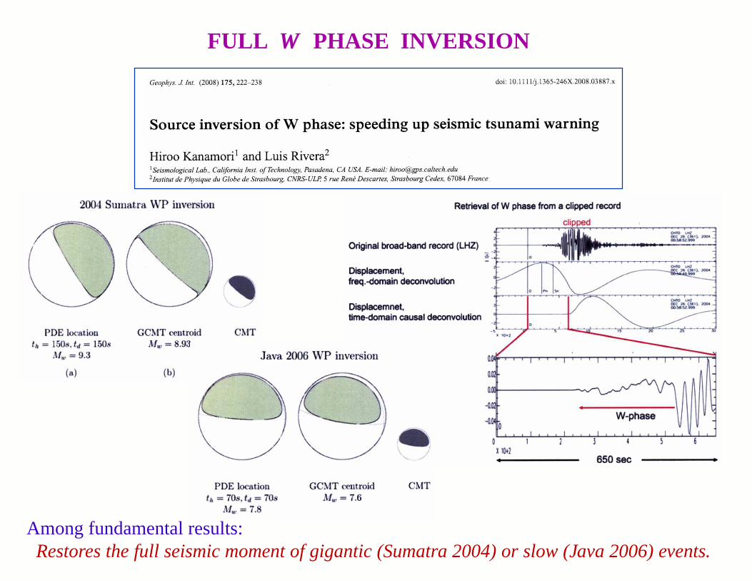
FULL WW PHASE INVERSION

Among fundamental results:Restores the full seismic moment of gigantic (Sumatra 2004) or slow (Java 2006) events.

BACK TO AN OLD-FASHIONED TIME−DOMAIN MA GNITUDE ?

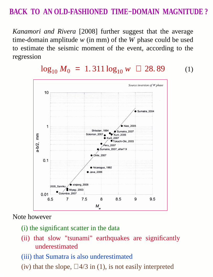
Kanamori and Rivera [2008] further suggest that the averagetime-domain amplitudew (in mm) of theW phase could be usedto estimate the seismic moment of the event, according to theregression

log10 M0 = 1. 311 log10 w + 28. 89 (1)

Note however

(i) the significant scatter in the data

(ii) that slow "tsunami" earthquakes are significantly underestimated

(iii) that Sumatra is also underestimated

(iv) that the slope,∼ 4/3 in (1), is not easily interpreted

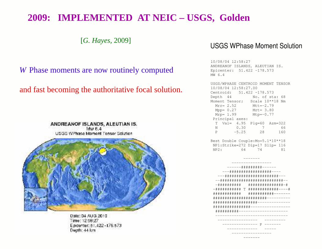
10/08/04 12:58:27 ANDREANOF ISLANDS, ALEUTIAN IS. Epicenter: 51.422 -178.573 MW 6.4

USGS/WPHASE CENTROID MOMENT TENSOR 10/08/04 12:58:27.00 Centroid: 51.422 -178.573 Depth 44 No. of sta: 68 Moment Tensor; Scale 10**18 Nm Mrr= 2.52 Mtt=-2.79 Mpp= 0.27 Mrt= 3.80 Mrp= 1.99 Mtp=-0.77 Principal axes: T Val= 4.95 Plg=60 Azm=322 N 0.30 7 66 P -5.25 28 160

Best Double Couple:Mo=5.1*10**18 NP1:Strike=272 Dip=17 Slip= 116 NP2: 64 74 81 ------- ----------------- ------#########------ ---##################---- ---#######################--- --###########################-- -########## ###############-# -########### T #############----# ############ ###########------- #######################---------- ###################-------------- ################----------------- ##########--------------------- ------------------------------- ----------------- --------- --------------- P ------- ------------- ----- ----------------- -------

2009: IMPLEMENTED AT NEIC – USGS, Golden

[G. Hayes,2009]

W Phase moments are now routinely computed

and fast becoming the authoritative focal solution.

USGS WPhase Moment Solution

How Well do These Various Algorithms Really Work ?

90˚

90˚

120˚

120˚

150˚

150˚

180˚

180˚

-150˚

210˚

-120˚

240˚

-90˚

270˚

-60˚

300˚

-30˚

330˚

-60˚ -60˚

-30˚ -30˚

0˚ 0˚

30˚ 30˚

60˚ 60˚

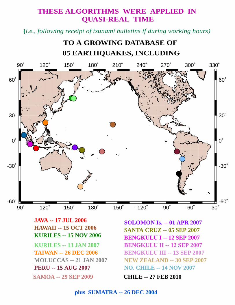
KURILES -- 13 JAN 2007TAIWAN -- 26 DEC 2006

PERU -- 15 AUG 2007NEW ZEALAND -- 30 SEP 2007MOLUCCAS -- 21 JAN 2007

SOLOMON Is. -- 01 APR 2007

BENGKULU I -- 12 SEP 2007BENGKULU II -- 12 SEP 2007BENGKULU III -- 13 SEP 2007

NO. CHILE -- 14 NOV 2007

SANTA CRUZ -- 05 SEP 2007

THESE ALGORITHMS WERE APPLIED INQUASI-REAL TIME

(i.e., following receipt of tsunami bulletins if during working hours)

JAVA -- 17 JUL 2006HAWAII -- 15 OCT 2006KURILES -- 15 NOV 2006

plus SUMATRA -- 26 DEC 2004

TO A GROWING DAT ABASE OF

85 EARTHQUAKES, INCLUDING

SAMOA -- 29 SEP 2009 CHILE -- 27 FEB 2010

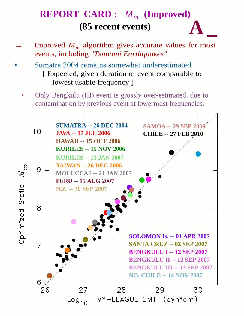
(85 recent events)

→→ Improved Mm algorithm gives accurate values for mostev ents, including"Tsunami Earthquakes"

• Sumatra 2004 remains somewhat underestimated[ Expected, given duration of event comparable to

lowest usable frequency ]

SUMATRA -- 26 DEC 2004JAVA -- 17 JUL 2006HAWAII -- 15 OCT 2006KURILES -- 15 NOV 2006

KURILES -- 13 JAN 2007TAIWAN -- 26 DEC 2006

PERU -- 15 AUG 2007N.Z. -- 30 SEP 2007

MOLUCCAS -- 21 JAN 2007

SOLOMON Is. -- 01 APR 2007

BENGKULU I -- 12 SEP 2007BENGKULU II -- 12 SEP 2007BENGKULU III -- 13 SEP 2007NO. CHILE -- 14 NOV 2007

SANTA CRUZ -- 02 SEP 2007

REPORT CARD : Mm (Impr oved)

A _

• Only Bengkulu (III) event is grossly over-estimated, due tocontamination by previous event at lowermost frequencies.

SAMOA -- 29 SEP 2009CHILE -- 27 FEB 2010

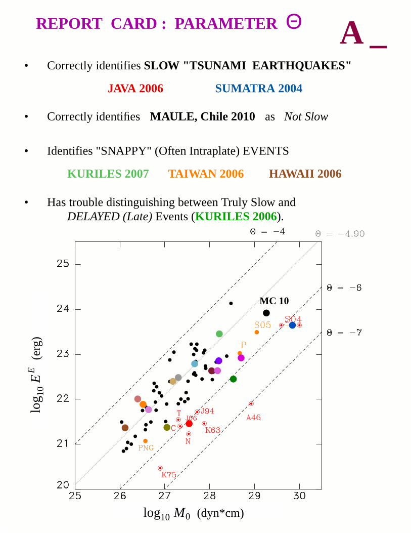
REPORT CARD : PARAMETER Θ A _• Correctly identifiesSLOW " TSUNAMI EARTHQ UAKES"

JAVA 2006 SUMATRA 2004

• Identifies "SNAPPY" (Often Intraplate) EVENTS

KURILES 2007 TAIWAN 2006 HAWAII 2006

• Has trouble distinguishing between Truly Slow andDELAYED (Late)Events (KURILES 2006).

log10 M0 (dyn*cm)

log 1

0E

E(e

rg)

• Correctly identifies MAULE, Chile 2010 as Not Slow

MC 10

Time-domain Computation Fourier-domain Computation

log10 M0 (dyn*cm) log10 M0 (dyn*cm)

Mm

p

Mm

p Mw

p

Mw

p

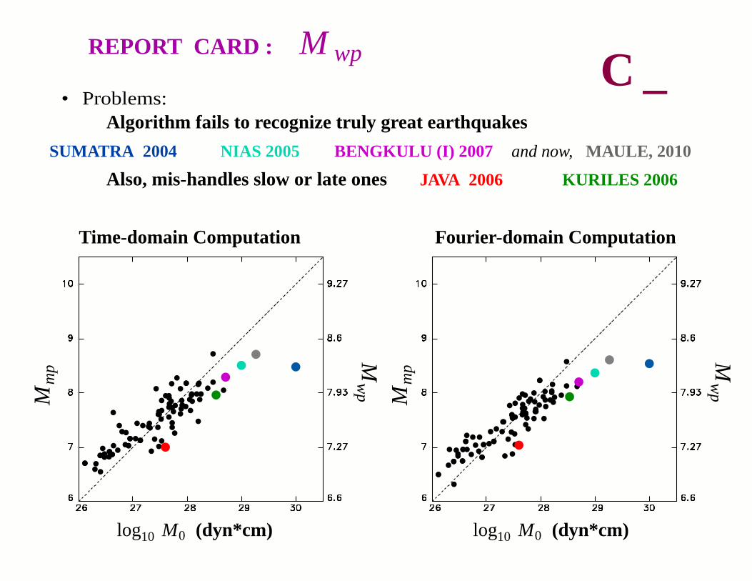
M wp

→→ IntegrateP −wave ground motion (in far field) to obtain seismic moment.

[In practice, integrate ground velocitytwice].

• Problems:Algorithm fails to recognize truly great earthquakes

Also, mis-handles slow or late ones

REPORT CARD :C _

SUMATRA 2004 NIAS 2005 BENGKULU (I) 2007

JAVA 2006 KURILES 2006

and now, MAULE, 2010

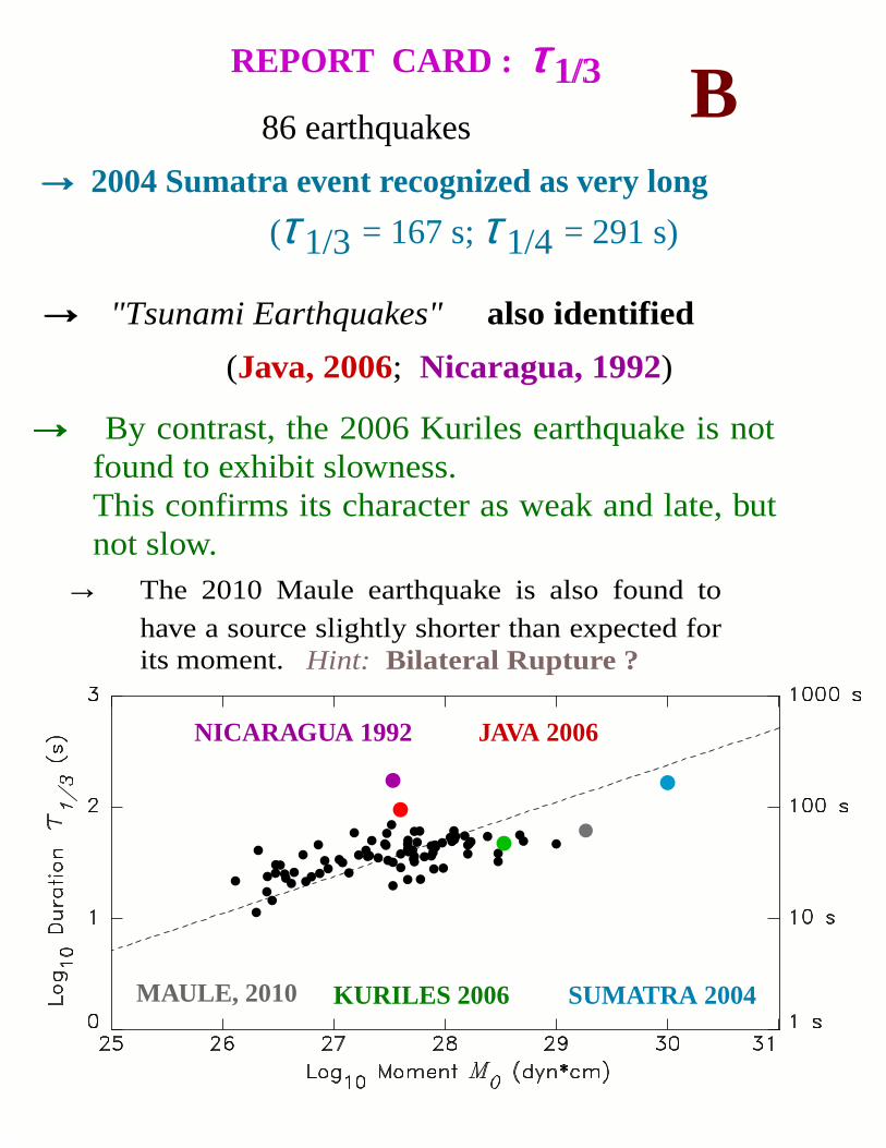
86 earthquakes

→→ 2004 Sumatra event recognized as very long

→→ "Tsunami Earthquakes" also identified

(τ 1/3 = 167 s;τ 1/4 = 291 s)

(Java, 2006; Nicaragua, 1992)

→→ By contrast, the 2006 Kuriles earthquake is notfound to exhibit slowness.This confirms its character as weak and late, butnot slow.

SUMATRA 2004

JAVA 2006NICARAGU A 1992

KURILES 2006

REPORT CARD : τ 1/3τ 1/3 B

→ The 2010 Maule earthquake is also found tohave a source slightly shorter than expected forits moment.

MAULE, 2010

Hint: Bilateral Ruptur e ?

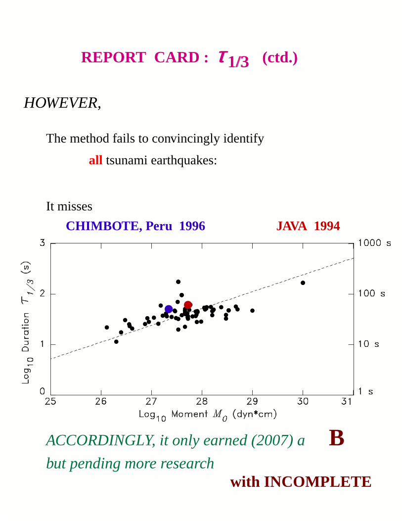
REPORT CARD : τ 1/3τ 1/3 (ctd.)

HOWEVER,

The method fails to convincingly identify

all tsunami earthquakes:

It misses

JAVA 1994CHIMBOTE, P eru 1996

ACCORDINGLY, it only earned (2007) a Bbut pending more research

with INCOMPLETE

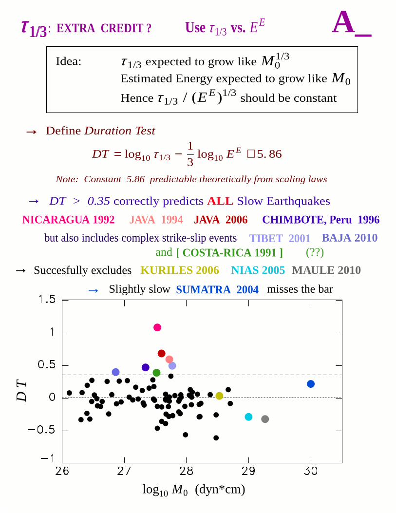
τ 1/3τ 1/3: EXTRA CREDIT ? Useτ 1/3 vs. EE

Idea: τ 1/3 expected to grow like M1/30

Estimated Energy expected to grow like M0

Henceτ 1/3 / (EE)1/3 should be constant

→→ DefineDuration Test

DT = log10τ 1/3 −1

3log10 EE + 5. 86

Note: Constant 5.86 predictable theoretically from scaling laws

DT > 0.35correctly predictsALL Slow Earthquakes

... but also includes one regular event (Costa-Rica, 1991)

log10 M0 (dyn*cm)

DT

NICARAGU A 1992 JAVA 1994 CHIMBOTE, P eru 1996

SUMATRA 2004

JAVA 2006

TIBET 2001[ COSTA-RICA 1991 ]

A_

but also includes complex strike-slip events BAJA 2010and (??)

Succesfully excludes KURILES 2006 NIAS 2005 MAULE 2010

Slightly slow misses the bar

→

→→

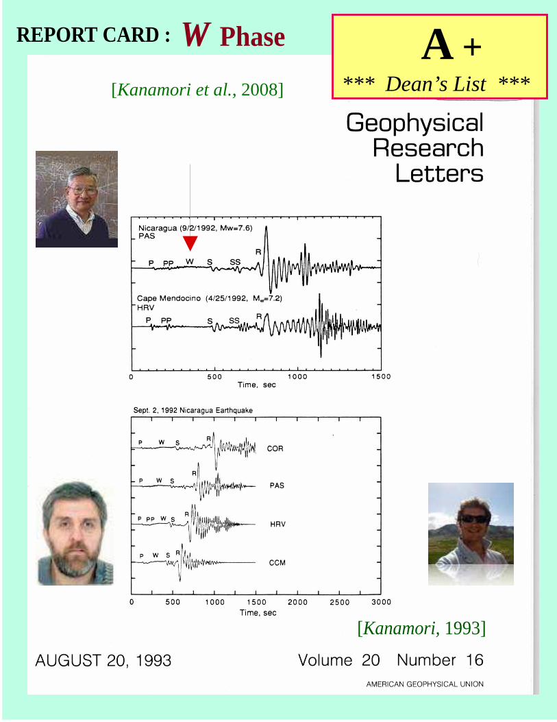
WWPhase

[Kanamori,1993]

A +*** Dean’ s List ***[Kanamori et al.,2008]

REPORT CARD :

DEFERRED STUDIES

Examples of Detailed Investigations of Earthquake Sources

→ Strictly Non Exhaustive !

84˚ 86˚ 88˚ 90˚ 92˚ 94˚ 96˚ 98˚ 100˚-2˚ -2˚

0˚ 0˚

2˚ 2˚

4˚ 4˚

6˚ 6˚

8˚ 8˚

10˚ 10˚

12˚ 12˚

14˚ 14˚

16˚ 16˚

18˚ 18˚

1

2

3

4

5

3.2

3.9

2.8

1.1

0.8

M0 (1029 dyn-cm)

93

163

281

379

490

Time Offset (s)

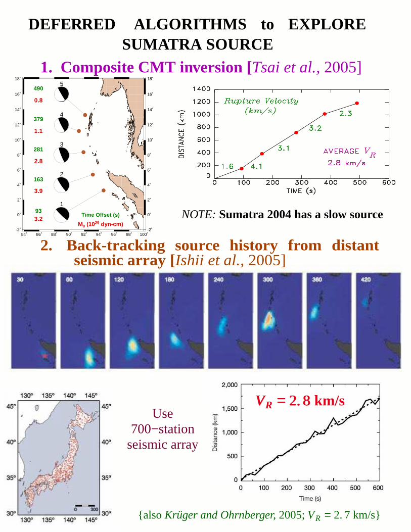
DEFERRED ALGORITHMS to EXPLORESUMATRA SOURCE

1. CompositeCMT in version [Tsai et al.,2005]

NOTE:Sumatra 2004 has a slow source

2. Back-tracking source history from distantseismic array [Ishii et al.,2005]

{also Kruger and Ohrnberger, 2005;VR = 2. 7km/s}

Use700−station

seismic array

VR = 2. 8VR = 2. 8km/s

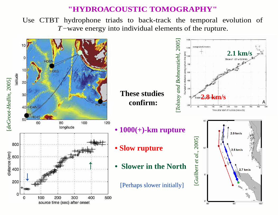
"HYDR OACOUSTIC TOMOGRAPHY"Use CTBT hydrophone triads to back-track the temporal evolution of

T−wav eenergy into individual elements of the rupture.

[de

Gro

ot-

He

dlin

,200

5]

[Tol

sto

y a

nd

Bo

hn

en

stie

hl,20

05]

[Gu

ilbe

rt e

t a

l.,20

05]

These studiesconfirm:

• 1000(+)-km rupture

• Slow rupture

• Slower in the North

[Perhaps slower initially]

2.8 km/s

2.1 km/s

↓↑

••

••

EVEN MORE DEFERRED

Reconstructing Focal Solutions

and Seismic Moments of Historical Earthquakes

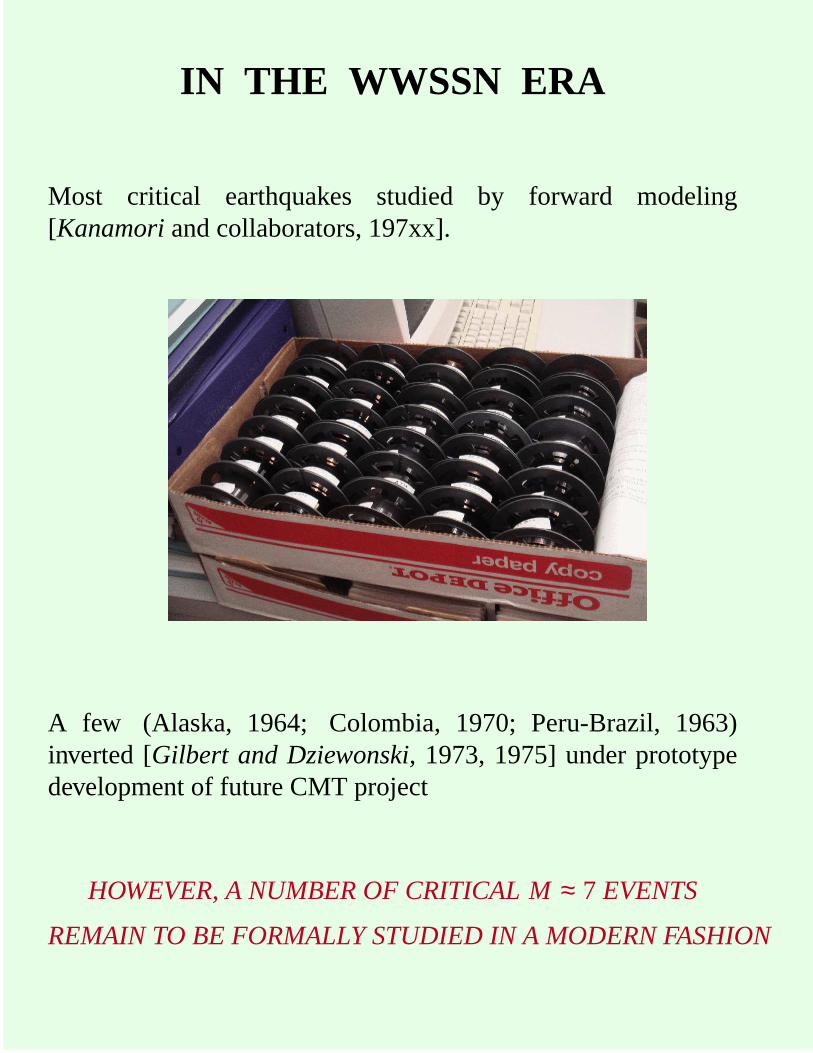
IN THE WWSSN ERA

Most critical earthquakes studied by forward modeling[Kanamoriand collaborators, 197xx].

A few (Alaska, 1964; Colombia, 1970; Peru-Brazil, 1963)inverted [Gilbert and Dziewonski,1973, 1975] under prototypedevelopment of future CMT project

HOWEVER, A NUMBER OF CRITICAL M≈ 7 EVENTS

REMAIN TO BE FORMALLY STUDIED IN A MODERN FASHION

IN THE PRE−WWSSN INSTRUMENTAL ERA

(1900 −1962)

Formal inversion becomes difficult because of the scarcity of data (and/or its poorazimuthal coverage), and the timing uncertainties affecting the spectral phases.

YET, THERE EXIST SUPERBLY ARCHIVED SEISMOGRAMS

WAITING TO BE ANALYZED

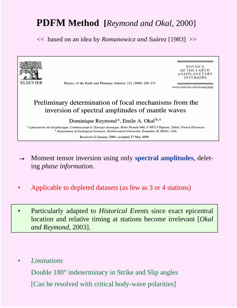
PDFM Method [Reymond and Okal,2000]

→→ Moment tensor inversion using onlyspectral amplitudes, delet-ing phase information.

• Applicable to depleted datasets (as few as 3 or 4 stations)

• Particularly adapted toHistorical Eventssince exact epicentrallocation and relative timing at stations become irrelevant [Okaland Reymond,2003].

• Limitations

Double 180° indeterminacy in Strike and Slip angles

[Can be resolved with critical body-wav epolarities]

<< basedon an idea byRomanowicz and Sua´rez[1983] >>

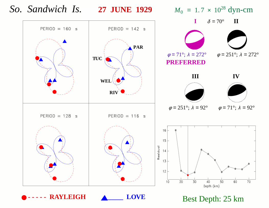
Best Depth: 25 km

M0 = 1. 7 × 1028 dyn-cm

- - - - - RAYLEIGH ______ LOVE

PAR

WEL

RIV

TUC

δ = 70°I II

III IV

φ = 71°; λ = 272° φ = 251°;λ = 272°

φ = 251°;λ = 92° φ = 71°; λ = 92°

27 JUNE 1929

PREFERRED

So. Sandwich Is.

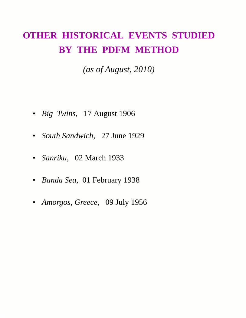
OTHER HISTORICAL EVENTS STUDIED

BY THE PDFM METHOD

(as of August, 2010)

• Big Twins, 17 August 1906

• South Sandwich,27 June 1929

• Sanriku, 02 March 1933

• Banda Sea,01 February 1938

• Amorgos, Greece,09 July 1956

BEFORE THE INSTRUMENTAL ERA

It is occasionally possible to obtain constraints on earthquake sourcesfrom the modeling of historical tsunami reports.

The three examples given provide significant insight into the potentialfor mega−quakes in the relevant subduction zones.

→→

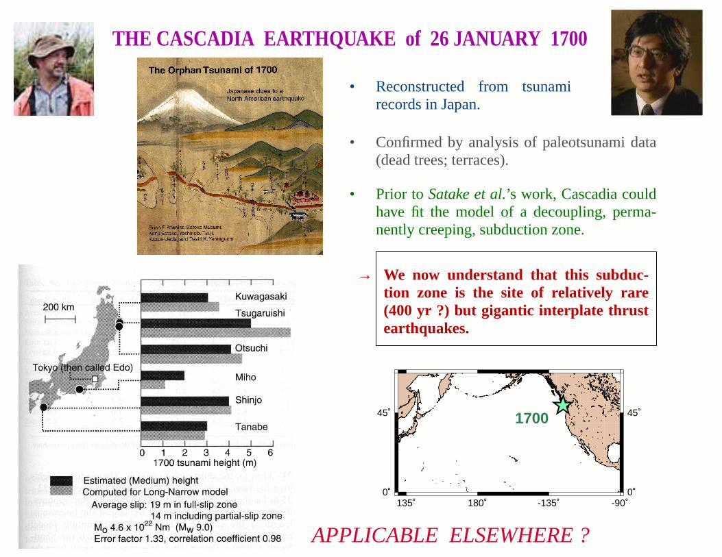
THE CASCADIA EARTHQ UAKE of 26 JANUARY 1700

• Reconstructed from tsunami records in Japan.

• Confirmed by analysis of paleotsunami data(dead trees; terraces).

• Prior to Satake et al.’s work, Cascadia couldhave fit the model of a decoupling, perma-nently creeping, subduction zone.

→ We now understand that this subduc-tion zone is the site of relatively rare(400 yr ?) but gigantic interplate thrustearthquakes.

135˚ 180˚ -135˚ -90˚0˚ 0˚

45˚ 45˚1700

APPLICABLE ELSEWHERE?

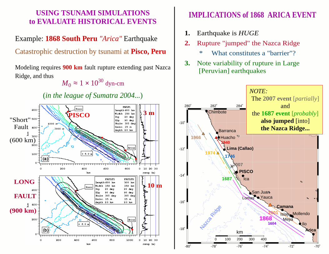
USING TSUNAMI SIMULATIONSto EVALUATE HISTORICAL EVENTS

Example:1868 South Peru"Arica" Earthquake

Catastrophic destruction by tsunami atPisco, Peru

Modeling requires900 km fault rupture extending past NazcaRidge, and thus

M0 ≈ 1 × 1030 dyn-cm

(in the league of Sumatra 2004...)

PISCO"Short"

Fault

(600 km)

LONG

FA ULT

(900 km)

3 m

10 m

-80˚

280˚

-78˚

282˚

-76˚

284˚

-74˚

286˚

-72˚

288˚

-70˚

290˚

-18˚

-16˚

-14˚

-12˚

-10˚

0 200 400100 300

km

19661940

1974

1687

20011868

1604

1746

Nazca

Rid

ge

PISCO

Lima (Callao)

Camana

AricaIlo

MollendoMejia

Islay

YaucaSan Juan

Lomas

Ica

Huacho

Barranca

Chimbote

2007

IMPLICATIONS of 1868 ARICA EVENT

1. Earthquake is HUGE

2. Rupture "jumped" the Nazca Ridge

* What constitutes a "barrier"?

3. Note variability of rupture in Large [Peruvian] earthquakes

NOTE:The2007 event [partially]

andthe1687 event [probably]

also jumped[into]the Nazca Ridge...

175˚

175˚

180˚

180˚

185˚

185˚

190˚

190˚

195˚

195˚

-30˚ -30˚

-25˚ -25˚

-20˚ -20˚

-15˚ -15˚

-10˚ -10˚

Fiji

Samoa

Tonga

Kermadec

18 NOV 1865

26 JUN 1917

30 APR 1919

01 MAY 1917

08 SEP 1948

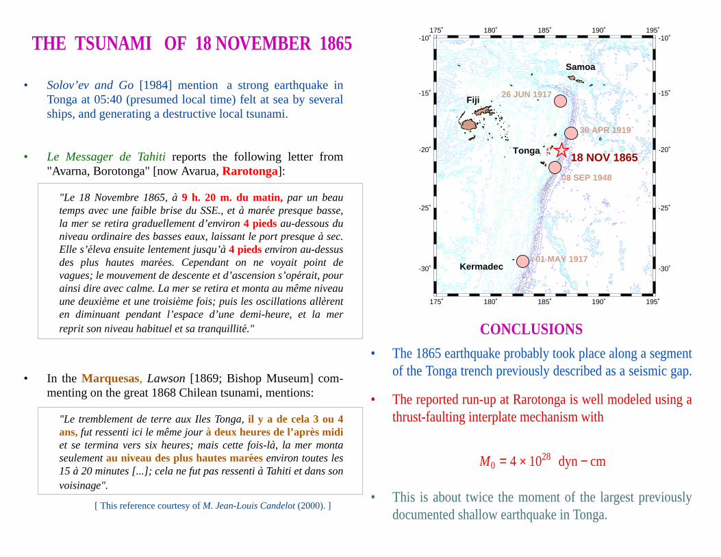
THE TSUNAMI OF 18 NOVEMBER 1865

• Solov’ev and Go [1984] mention a strong earthquake inTonga at 05:40 (presumed local time) felt at sea by severalships, and generating a destructive local tsunami.

• Le Messager de Tahiti reports the following letter from"Avarna, Borotonga" [now Avarua,Rarotonga]:

"Le 18 Novembre 1865, a9 h. 20 m. du matin, par un beautemps avec une faible brise du SSE., et a` mare epresque basse,la mer se retira graduellement d’environ 4 pieds au-dessous duniveau ordinaire des basses eaux, laissant le port presque a` sec.Elle s’eleva ensuite lentement jusqu’a` 4 piedsenviron au-dessusdes plus hautes mare es. Cependant on ne voyait point devagues; le mouvement de descente et d’ascension s’ope´rait, pourainsi dire avec calme. La mer se retira et monta au meˆme niveauune deuxie`me et une troisieme fois; puis les oscillations alle`renten diminuant pendant l’espace d’une demi-heure, et la merreprit son niveau habituel et sa tranquillite´."

• In the Marquesas, Lawson[1869; Bishop Museum] com-menting on the great 1868 Chilean tsunami, mentions:

"Le tremblement de terre aux Iles Tonga, il y a de cela 3 ou 4ans,fut ressenti ici le meˆme jour a deux heures de l’apres midiet se termina vers six heures; mais cette fois-la`, la mer montaseulementau niveau des plus hautes mareesenviron toutes les15 a20 minutes [...]; cela ne fut pas ressenti a` Tahiti et dans sonvoisinage".

[ This reference courtesy ofM. Jean-Louis Candelot(2000). ]

CONCLUSIONS

• We confirm beyond doubt that the 1865 earthquake inTonga produced a tsunami resulting in far-field flooding.

• The 1865 earthquake probably took place along a segmentof the Tonga trench previously described as a seismic gap.

• The reported run-up at Rarotonga is well modeled using athrust-faulting interplate mechanism with

M0 = 4 × 1028 dyn− cm

• This is about twice the moment of the largest previouslydocumented shallow earthquake in Tonga.

AS FOR THE FUTURE....

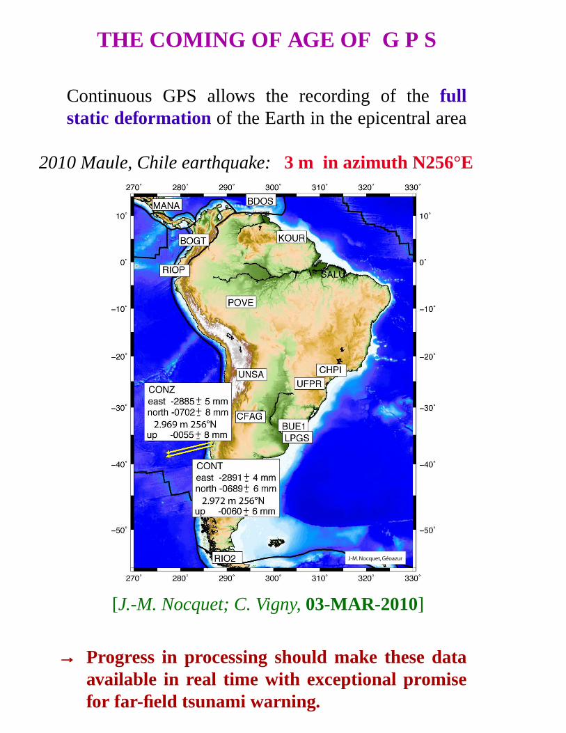
THE COMING OF AGE OF G P S

Continuous GPS allows the recording of thefullstatic deformation of the Earth in the epicentral area

2010 Maule, Chile earthquake: 3 m in azimuth N256°E

[J.-M. Nocquet; C. Vigny,03-MAR-2010]

→→ Progress in processing should make these dataav ailable in real time with exceptional promisefor f ar-field tsunami warning.

AS FOR THE FUTURE....

The future of Long-Period Seismology maybe at UNAVCO...