DI

SC

US

SI

ON

P

AP

ER

S

ER

IE

S

Forschungsinstitut zur Zukunft der ArbeitInstitute for the Study of Labor

The Role of Mothers and Fathers in Providing Skills: Evidence from Parental Deaths

IZA DP No. 5425

January 2011

Jérôme AddaAnders BjörklundHelena Holmlund

The Role of Mothers and Fathers in Providing Skills:

Evidence from Parental Deaths

Jérôme Adda European University Institute

and IZA

Anders Björklund SOFI, Stockholm University

and IZA

Helena Holmlund SOFI, Stockholm University

Discussion Paper No. 5425 January 2011

IZA

P.O. Box 7240 53072 Bonn

Germany

Phone: +49-228-3894-0 Fax: +49-228-3894-180

E-mail: iza@iza.org

Any opinions expressed here are those of the author(s) and not those of IZA. Research published in this series may include views on policy, but the institute itself takes no institutional policy positions. The Institute for the Study of Labor (IZA) in Bonn is a local and virtual international research center and a place of communication between science, politics and business. IZA is an independent nonprofit organization supported by Deutsche Post Foundation. The center is associated with the University of Bonn and offers a stimulating research environment through its international network, workshops and conferences, data service, project support, research visits and doctoral program. IZA engages in (i) original and internationally competitive research in all fields of labor economics, (ii) development of policy concepts, and (iii) dissemination of research results and concepts to the interested public. IZA Discussion Papers often represent preliminary work and are circulated to encourage discussion. Citation of such a paper should account for its provisional character. A revised version may be available directly from the author.

IZA Discussion Paper No. 5425 January 2011

ABSTRACT

The Role of Mothers and Fathers in Providing Skills: Evidence from Parental Deaths*

This paper evaluates the long-term consequences of parental death on children’s cognitive and noncognitive skills, as well as on labor market outcomes. We exploit a large administrative data set covering many Swedish cohorts. We develop new estimation methods to tackle the potential endogeneity of death at an early age, based on the idea that the amount of endogeneity is constant or decreasing during childhood. Our method also allows us to identify a set of death causes that are conditionally exogenous. We find that the loss of either a father or a mother on boys’ earnings is no higher than 6-7 percent and slightly lower for girls. Our examination of the impact on cognitive skills (IQ and educational attainment) and on noncognitive skills (emotional stability, social skills) shows rather small effects on each type of skill. We find that both mothers and fathers are important, but mothers are somewhat more important for cognitive skills and fathers for noncognitive ones. JEL Classification: J12, J17, J24 Keywords: family background, cognitive and noncognitive skills, parental death Corresponding author: Anders Björklund Swedish Institute for Social Research (SOFI) Stockholm University SE-10691 Stockholm Sweden E-mail: anders.bjorklund@sofi.su.se

* We are grateful to Andreas Bergh, David Card, Christian Dustmann, Andrea Ichino, Costas Meghir, Emmanuel Saez, Chris Taber and seminar and workshop participants at CEPR Family Economics workshop in Bergen, Autonoma, IFAU Uppsala, IZA, Linnaeus University, London School of Economics, Lund University, Statistics Norway and Stockholm University for comments. Martin Hällsten provided clever advice about data. Financial support from Swedish Council for Working Life and Social Research (FAS) and Jan Wallander and Tom Hedelius Foundation is gratefully acknowledged.

2

I. Introduction

The loss of a parent is probably one of the most traumatic events a child can experience. It is likely

to affect the child detrimentally in many ways, by depriving her of love, care, guidance and

discipline. It represents not only an emotional shock but also a loss in parental inputs and a

permanent shock to family income, which can have long-lasting consequences. While orphanage is

a widespread phenomenon in developing countries, due to wars, epidemics and poor health, it is not

such a rare event in developed countries either. According to statistics published by UNICEF in

2007, 2.8 million children aged 0 to 17 had lost a parent in the United States, and about 3.8 million

in the European Union.

The effect of growing up with only one parent has been extensively studied in economics and other

social sciences. The literature has most often focused on the effect of divorce and found large

negative effects from cross-sectional studies (see e.g. McLanahan 2004). Children growing up in

single-parent households are more likely to drop out of school, experience teen-age pregnancies or

unemployment later on. As noted by many researchers in this field, these differentials are not likely

to be causal as divorce is correlated with family traits that determine long-term outcomes of

children. Some studies have therefore focused on parental death, mainly seen as an outcome that is

more exogenous than divorce.1 These studies are usually limited because parental death is poorly

captured in survey data. Despite the difficulty in establishing causal effects, this literature has in

part inspired policy in many countries, in which the role of both parents (and usually the father) are

encouraged in order to achieve better outcomes for children. For instance, this is the case with the

Head Start-Family and Community Partnerships in the US and the Healthy Marriage Initiative run

by the US Department of Health since 1996.

In this paper, we evaluate the long-term consequences of parental death on children and we improve

on the existing literature in several important ways. First, we show that, similarly to divorce,

parental death is not an exogenous event when it comes to child development. The causes of death

at early ages are particular, with an over-representation of suicides and accidents. These early

deaths are often correlated with socio-economic status of the family and as such, simple cross-

sectional estimates will be subject to selection bias. We therefore develop a novel econometric

method to get a consistent estimate of the causal effect of parental death. The method is similar in

1 Examples of these studies are Corak (2001) on Canadian data, Lang and Zagorsky (2001) who use the NLSY and Francesconi et al. (2010) using the German Socio-Economic Panel. Björklund and Sundström (2006) study the effect of divorce in Sweden using a family fixed effect methodology.

3

spirit, but distinct from the one proposed in Altonji et al. (2005). We exploit the fact that some of

our outcomes are realized at a particular moment in time (such as cognitive tests or schooling). We

assume that the endogeneity of early death is constant or decreasing with the age of the child during

childhood. This assumption is motivated by data on causes of early deaths. We show that these two

elements are enough to construct a consistent estimate, or at least an upper bound (in absolute

value) for the true effect. This method also allows us to test for the endogeneity of particular causes

of death and to construct a subset of our sample with causes that are exogenous, conditional on a

rich set of observed characteristics. We also compare our results with those obtained through a

family fixed effect estimator.

Second, we use data on a very large random sample of individuals born in Sweden in 1953-1967,

obtained from administrative records, which allows us to exploit information on long-run outcomes

of children who experienced bereavement, including formal education levels, income, IQ scores and

measures of social skills. We are thus able to evaluate the effects on a broader set of outcomes than

the previous literature. This is important because parents, and parental death, may affect many types

of skills, some of which are non-cognitive in nature.

Third, we test whether parents are essential to the long-term development and skills of their

children, and whether there are specific effects of fathers or mothers on sons and daughters. The

specific role of fathers and mothers in raising children has long been debated in the social science

literature, without a clear consensus. Studies usually find a positive effect of father’s involvement,

and it is often hypothesized that fathers have a role as a model, especially towards sons.2 Some

studies find a specific role for fathers in shaping long-run empathy (Koestner et al. 1990). However,

this literature lacks a clear source of variation in parenting to establish causal relationships.

Haveman and Wolfe (1995) suggest that the role of mother’s education is particularly important for

children’s educational achievement, but more recent evidence in Holmlund et al. (2011) show that

once selection is accounted for, it is not clear that one parent’s education is more important than the

other’s. We are able to investigate the specific roles of fathers and mothers as our sample is large

enough to conduct separate analysis by gender. This is a topic that is difficult to address with data

on divorce as, most often, the custody of the children is given to mothers.

2 However, this effect often disappears when controlling for the role mothers play see Amato and Rivera (1999), Conner et al. (1997).

4

Fourth, as we argue below, parental death has complex implications on the production of skills of

the children. In addition to psychological distress, the child suffers from lack of input of the

deceased parent and reduced family income. However, the remaining parent or the extended family

may compensate in part for the loss. Given the quality of our data, we are able to control and

analyze part of these mechanisms, including the role of income in mediating the effect of parental

death, as well as re-partnering.

We first show that parental death has surprisingly small average effects on cognitive outcomes,

despite representing a traumatic shock. Given the size of our dataset, we can rule out zero effects,

but our preferred estimates represent a loss of a couple of months of schooling. As we observe

family income, including potential transfers after a death, we evaluate the role of income in

producing human capital. Our results do not support a leading role for income in the human capital

production function.3

Second, we show that the death of either the mother or the father has effects in particular on their

sons’ income and earnings during adulthood over and above the effect on educational attainment

and IQ. For sons this effect is around six percent for earnings. We take this larger earnings effect as

an indication that there are also effects on noncognitive skills. To explore this hypothesis, we

continue to examine effects on noncognitive skills as measured by the psychological profile at

military enlistment. We also explore this issue further by looking at the impact of deceased parents

on health-related behavior, and on subsequent family formation. Our results suggest that there are

negative effects of the death of either the father or the mother on such outcomes, but they are not

large.

Third, we compare the relative impact of bereavement of the mother and the father. The estimated

effects on earnings and income are about the same, but there is a tendency that the mother is more

important for cognitive skills, and the father is more important for our noncognitive outcomes.

Finally, we examine whether the effects are heterogenous in various dimensions. We explore the

effects of parental death at various ages of the child. We show that such an event can influence

cognitive skills even during teenage years, which suggests that cognitive skills are not totally

determined at a young age.

3 Carneiro and Heckman (2002) examine liquidity constraints in post-secondary schooling and show the importance of long-run family effects rather than liquidity constraints.

5

The paper is organized as follows. Section II presents the conceptual framework and a novel

econometric methodology to tackle endogeneity bias. Section III describes the data sources we use

and details the institutional features in Sweden. Section IV presents the effects of parental death on

cognitive skills and Section V shows the effects on noncognitive skills. Section VI discusses effect

heterogeneity in various dimensions. Section VII presents results from family-fixed effects and

Section VIII concludes.

II. Conceptual Framework and Econometric Methodology

A. Conceptual Framework and Overview of the Literature

Following Ben-Porath (1967), the economic literature has modeled the acquisition of skills using a

production function, where inputs are the child’s innate ability, parental inputs and school quality.

Becker and Tomes (1979) present a model in which parents decide optimally how to invest in their

children’s human capital. Investment in this model operates through the budget constraint.

Liebowitz (1974) also includes home investment in children and tests to which extent time spent

with the child reading or playing matters for cognitive achievements. More recent studies have

emphasized the dynamic aspect of the acquisition of skills, meaning that skills acquired early in life

help to develop skills later on (Todd and Wolpin 2003, Caucutt and Lochner 2004, Todd and

Wolpin 2007, Cunha and Heckman 2008, or Cunha et al. 2010). This approach follows the

advances in other fields such as psychology and human biology. It also stresses the importance of

early interventions to promote human capital in adulthood.

In this literature, few studies look at the specific roles of mothers and fathers. Rosenzweig and

Wolpin (1994) investigate the effect of mother’s education on children’s cognitive outcomes.

Altonji and Dunn (1996) look at the effect of parental education on the child’s return to education.

They conclude that whereas the education of the parents matters to determine the level of human

capital and wages, there is no strong relationship between parental education and the return to

schooling.

A number of papers have attempted to measure the effect of maternal employment on children’s

outcomes, without reaching a consensus (Blau and Grossberg 1992, Parcel and Menaghan 1994,

Bernal 2008, Bernal and Keane 2010). This is perhaps not surprising because maternal employment

is a choice that may depend on the child’s ability or potential ability and may therefore be

6

endogenous.4 Similarly, it is well established that children growing up in single-parent households

acquire less human capital. However, divorce may also be endogenous, making it difficult to

establish a causal link between the lack of input of one parent and human capital. Lang and

Zagorsky (2001) stress that point. Using data from the NLSY, they regress various child outcomes

on the presence of parents during childhood and family controls such as parental education and

alcoholism. As the results could still be subject to omitted-variable bias, they also investigate the

effect of parental death for a subset of their data. Parental death is taken to be exogenous. A similar

point is made by Corak (2001) who investigates the effect of parental death on labor market

outcomes for children who lost one of their parent in late adolescence (aged 17 to 19). In a different

context, Gertler et al. (2004) exploit cross-sectional data from Indonesia to investigate the effect of

parental death on school performance.5 Due to the nature of the data, they can only look at short-run

effects. In this paper, we extend these results using a considerably larger dataset, which allows us to

probe the assumption of the exogeneity of parental death.

The previous literature in psychology and in economics has also emphasized that skills are multi-

dimensional. The early economic literature puts more emphasis on cognitive skills, such as reading

or mathematical skills, and has shown how these skills are rewarded in the labor market. More

recently, economists have stressed that other skills are important as well, such as motivation and

drive, the ability to trust or social skills (Heckman et al. 2006, Butler et al. 2009, Lindqvist and

Vestman 2011).

To understand child-skill formation, we take a reduced form view of the production function, where

we do not detail the particular choices of parents such as specific child expenditures or choice of

schooling. Given the nature of our data, we do not model the dynamics of human capital. Denote Si

a vector of skills acquired by the individual at the end of childhood. These skills comprise cognitive

measures such as education or measures of IQ, or noncognitive ones such as responsibility and

emotional stability. We relate skills to parental inputs and family resources such as:

, , , , , , (1)

where Ai is the child’s innate ability, Mi, Fi and Oi are the time investments of the mother, the father

and other members of the family through adulthood (defined as through age 18 in our empirical

application), Yi is total family income during childhood and Wi is a psychological well-being indicator. 4 Dustmann and Schönberg (2010) for Germany and Liu and Nordstrom Skans (2010) for Sweden use reforms that expanded maternity leaves to investigate the causal long-run effect on schooling of mothers’ time spent with their babies. 5 Several authors have studied the effect of parental death in developing countries, see also Case and Ardington (2006) and Chen et al. (2009).

7

We assume that the skills of the child are a weakly increasing function of all its arguments. We index

the production function with the subscript i as the returns could be heterogeneous. For instance, it is

possible that parental inputs have different effects depending on the sex of the child.

To investigate the effect of the death of a parent, for instance the mother, consider the total differential

of (1):

∆ ∆ ∆ ∆ ∆ ∆ (2)

where ∆ , , , , , refers to the change in a variable during childhood in case of the

death of the mother. We now discuss the sign of ∆ and its various components.

First, death affects children negatively through distress, i.e. WiDM 0. The amount and

susceptibility of distress is most likely heterogeneous across children. One dimension of

heterogeneity may be age. Results from the psychology literature suggest that very young children

may not be able to remember such an event as episodic memory does not stabilize before the age of

four or five (Tulving 1983).

In the case of the death of the mother, clearly ∆ <0 as the child is deprived of maternal inputs

from the date of the death. The effect through the other channels is more difficult to sign. For

instance, the father can compensate the loss of input of the mother by reducing his own leisure time

or hours worked and increase his own inputs. Alternatively, he may have to decrease his parental

inputs if priority is given to compensate for the loss in family income. Hence, the sign of ∆ is

ambiguous. If the mother was working, her death represents a loss in family income, although the

spouse, government transfers or insurance policies may compensate part of that loss. We discuss in

detail below these various transfers and show that empirically, ∆ 0 . Finally, following death,

other people may step in to replace the deceased parent, such as grandparents or a new partner.

However, it is also possible that the death of a parent results in less contacts with the relatives of the

deceased family member, or that the presence of a step-parent creates a “Cinderella” effect. Thus,

the sign of ∆ is indeterminate.

In the case of the death of the father, the effect should be qualitatively the same, although the shock

to income is expected to be more important as men were more likely to work during the period we

study and earned a larger share of family income.

8

Abstracting from grief, if the allocation of resources were optimal before death, then ∆ | 0.

Bereavement aggravates this effect but is difficult to measure. Thus, the effect of parental death on

children captures many components but we cannot fully separate all of them. Our dataset allows us

to shed light on some of the effects involved, as we are able to reconstruct family income during

childhood, inclusive of transfers that are received upon death to the remaining spouse and the

children. We are also able to control for re-partnering as one of the channels involved. However, we

cannot separate the effects of lack of parental investment and bereavement but both tend to worsen

the outcome of the child, so we are able to recover the sum of the two. This combined effect can

also be considered as a bound on the parental input effect, which will be particularly informative if

the combined effect is small.

Cunha and Heckman (2007) model the production function as a CES function of inputs and discuss

two polar cases. Under perfect substitution, neither parent is critical to the child’s development, as

mother’s input can replace father’s input and vice-versa. Under perfect complementarity, parental

death has a marked effect on the acquisition of skills as the deceased parent’s skills cannot be

replaced. Our framework allows us to test this latter case, i.e. whether either parent is essential to

the development of particular skills of their children.

B. Econometric Methodology

Let Si denote an outcome for the child, such as years of completed education, a measure of IQ or,

abusing our definition of skills, earnings as an adult. Let Di be an indicator variable equal to one if one

of the parents died before the child reached 19 and Xi a vector of pre-determined child and family

characteristics. We aim at estimating the following relationship:

Si 0 Di Xi ui (3)

The parameter represents the total effect of parental death as discussed in the previous section.

We aim at disentangling some of the effects by controlling for some of the channels such as family

income or re-partnering. In this case the parameter is to be interpreted as the effect of changes in

parental inputs together with the psychological effect of bereavement.

As discussed in the introduction, an early death is not necessarily an exogenous event. Figures 1a

and 1b show the prevalence of some selected causes of death as a function of the age of the child

when this death occurs, for mothers and for fathers. At a young age, there is an over-representation

9

of deaths from suicides, homicides and accidents, the former representing around 15 percent of all

deaths. In the case of fathers, accidents represent up to 40 percent of all cases at a young age. Work-

related accidents occur proportionally more often in blue-collar occupations. Road accidents are

more likely to occur when consuming alcohol. It is likely that the conditions that lead to such deaths

are correlated with long-run child outcomes, even after conditioning on a rich set of family and

parental characteristics. 6

The econometric toolbox provides us with several ways to tackle endogeneity. The most commonly

used is instrumental variables. In our case, it is difficult to find a convincing instrument that

influence early death, but not children’s outcomes per se. We have already made a case that

accidents may not be totally exogenous, and it is difficult to argue a priori that a particular cause of

death is not linked to behavior and therefore to child outcomes.

A second method, which has been used in a similar context by Chen et al. (2009) is to exploit the

outcome of siblings, by controlling for family fixed effects. This technique has also been used in the

divorce literature (see Björklund and Sundström 2006 or Amato 2010). It is worthwhile to point out

how the coefficient of interest is identified. The effect of death is identified through families with at

least two children of age below and above eighteen. The effect of parental death may be different

for these families for at least two reasons. First, given the spacing of birth, the younger sibling is

likely to be close to eighteen as well, so the sample of children used for identification is rather old.

If cognitive and non-cognitive skills are acquired early on, the effect of parental death may be small

for this particular sample. Second, the older sibling, being adult, may step in and take on the role of

the deceased parent, providing skills or resources, which would lead again to an attenuation of the

effect. Thus, it is doubtful that the fixed effect estimates can be extrapolated to the whole sample.

Indeed, it turns out that in our data the identifying sample of siblings reveal a cross-sectional pattern

that is markedly different from the main representative sample. In Section VII we report the results

for the fixed-effect approach as a comparison.

Given the limitations of the more traditional econometric methods, we develop a novel approach to

deal with the endogeneity of death. We detail the procedure below.

6 Erikson and Torssander (2008) examine the unconditional association between social class and around 50 cause-specific deaths, using large Swedish register data covering deaths from 1991-2003. They find a clear mortality gradient for the majority of causes although the strength of the association varies. Causes of death for which higher social classes have higher death risks are practically non-existent.

10

Denote by Pi an auxiliary variable equal to one if the child experienced the death of a parent “just”

after completing education or taking an IQ test. In practice, we consider an interval of a few years.

For ease of exposition, we use age 18 as a cut-off, although in the empirical application we vary this

age limit depending on the outcome.

As the outcome is already determined before that event, there is no causal link between the

auxiliary variable Pi and the outcome Si. In a different context, the empirical literature has often

used such “placebo” variables to evaluate the robustness of the results. We use it here in a different

way, as it will allow us under some conditions to estimate the bias and construct an unbiased

estimator

Denote corr(Di,ui) X the (unobserved) correlation between the indicator variable for parental death

and the error term, conditional on a set of characteristics X. Define the ratio of the correlation

between parental death after childhood and during childhood as: , |

, | (4)

Identifying assumption: We assume that the correlation between parental death before 18 and

unobserved family traits is larger or equal to the correlation between parental death shortly after 18

and those family traits:

1 (5)

The motivation for such an assumption comes from the evidence displayed in Figures 1a and 1b.

There is no sharp discontinuity in the causes of death when children reach adulthood, and we do not

observe a peak in mortality around that age. In a neighborhood around that age range, we believe it

is reasonable to assume that 1. At earlier ages, given that we observe more deaths due to causes

such as suicides, it is likely that parental deaths are more endogenous than at a later age. This

assumption can also be rationalized within the context of a duration model until parental death with

unobserved heterogeneity, which is correlated with the process of skill acquisition of the child. In

such a setup, the families who experience an early death are negatively selected, compared to those

with a later death. Including the variable Pi in equation (3), we get:

Si 0 Di Pi Xi ui (6)

where =0 as Pi has no causal effect on Si . Denote ˆ the (potentially biased) OLS estimate of the

effect of parental death before education is completed and by ˆ the OLS effect of parental death

after education is completed or after IQ is measured. Using assumption (5) and the identity (4), after

11

some straightforward algebra, we derive an unbiased estimator for , as:

ˆ ˆ ˆ (D,P,) ˆ (7)

with

(D,P,) Var(P) cov(D,P)

Var(P)Var(D)

Var(D)Var(P) cov(D,P) (8)

This estimator converges to the true value :

E ˆ ˆ and Var( ˆ ˆ ) Var( ˆ ) (D,P,)2Var( ˆ ) 2(D,P,)cov( ˆ , ˆ ) (9)

We refer the reader to Appendix A.1 for a formal proof. The unbiased estimator is easy to derive as

it only involves a linear transformation of the OLS coefficients and moments from the data.

This estimator is similar in spirit to the one derived in Altonji et al. (2005). They instead make the

assumption (in our notation):

corr(Di,ui) corr(Di,Xi)

This expression means that the correlation of parental deaths with the error term is the same as the

one between the observable characteristics and parental death. They show that this is true if a large

number of observable characteristics are drawn at random from the list of all potential explanatory

variables. Our estimator relies instead on the property that our outcome variable is determined at a

given point in time. 7 In the result section below, we report estimates based on the assumption

1. We note that in our data, / 0, so that our estimates are an upper (absolute) bound if

1. This way of proceeding is similar in spirit with Altonji et al. (2005).

Note that in our empirical application, when calculating our unbiased estimator, we subtract ˆ

coefficients that might not be statistically different from zero. Therefore, it is possible that, in finite

distance, our methodology reduces the effect by more than the omitted-variable bias, which leads to

too small estimates. A Monte Carlo simulation reported in Appendix A.2 confirms that our

estimator has this property for sample sizes of about 1,000 observations For larger samples such as

those used in our empirical analysis, the small sample bias appear to be very small.

7 Note that our estimator is different from a regression discontinuity design (see Angrist and Krueger 1991, Angrist and Lavy 1999, Hahn et al. 2001, Imbens and Lemieux 2008 among others) as it is not a simple difference of the outcome across the boundary. Identifying the effect of parental death at the boundary (age 18 for instance) would be difficult as the treated individual would have spent her entire childhood with her parents, and can hardly be labeled as treated. We should expect (and indeed find) no discontinuity at the boundary. Note also that our estimator is different from the proxy method (see for instance Wickens 1972), because the introduction of the variable Pi does not lead to an unbiased estimator of in equation (5) and does not reduce the bias either.

12

From assumption (5), we can derive an estimator of the covariance between early parental death and

the error term:

cov(D,u) ˆ Var(D)Var(P) cov(D,P) (10)

We use this expression to test the assumption of no endogenity, which amounts to test for the

significance of the auxiliary variable Pi. We can also use this expression to test for the endogeneity

of particular causes of death. It is possible that when conditioning on a rich set of observed

characteristics, some particular causes of death are not related to unobserved determinants of skills.

If such a subset exists, we can then use it to consistently estimate the causal effect directly through

OLS using equation (3). In our result section, we present results based on a subset of causes of

death, for which we have established no endogeneity (conditional on covariates) in the case of

education or IQ scores. We refer the reader to this section for a description of how we construct

such a sample using a heuristic method.

Identifying exogenous death causes is useful as our econometric methodology described in (7)

relies on the timing of the outcome. While we can argue that assumption (5) should hold when we

consider IQ tests taken at age 18, it is more difficult to argue for an outcome such as labor earnings

measured during adulthood, when some of the observed individuals are in their fifties. We cannot

rule out that parental death occurring before we measure labor market performance has no influence

on wages. In other words, we cannot define a credible auxiliary variable for this outcome and use

the procedure detailed above. Hence, our strategy to control for endogeneity in some of our

outcomes such as labor income or family formation is to rely on a subset of causes of death, for

which we have shown that there is no endogeneity in the case of education or IQ scores.

The interpretation of these estimates depends on the assumption on how parental death impacts on

the production of skills. In one polar case the production function depends on parental death (as

shown in (2)), but not on the particular cause of death. This would allow us to generalize our results

to all causes. However, this would not be true if some particular causes of death are more

traumatizing than others. It may be the case that deaths due to suicides or accidents have a bigger

emotional impact than deaths due to infectious diseases. In this case, our estimates are local and

conditional on the set of causes we consider.

13

III. Institutional Setting and Data

A. Institutional Setting for Sweden

Our study covers deaths that took place during 1971-1985. In order to interpret our results, we need

to have a clear picture of the support provided to the surviving spouse and the children during this

period of time. This support has many interacting components each of which is quite complex.

Thus, we are only able to offer a sketchy account of the situation for single parents during this

period of time.

First of all, public policy provided support for full- or halftime working single parents. Our period

of study overlaps with a period of rapidly growing supply of childcare slots for working and

studying parents. In addition, the supply of after-school care for young school children (up to

around age 10) rose rapidly over the period. Both types of care were heavily subsidized by the

municipalities that were the main providers; the subsidies were generally larger for single-parent

families and for families with several children. During the first part of this period, many Swedish

families with young children faced restrictions to these types of child care due to excess demand at

existing prices. However, the municipalities applied rules that gave priority to children of single-

parented families. Thus, we argue that the prospects for a surviving parent to work fulltime in the

labor market were good in Sweden in this period. Female labor force participation rose rapidly

during the period and was high by most international standards. At the time, it was considered

natural for a widow to strive for a full-time (or slightly less than full-time) job.

Second, the overall Swedish social insurance system offered a set of pension schemes for the

surviving spouse and the children.8 The overall Swedish system can be considered as having two

main parts, namely (i) the compulsory public one determined by the parliament and (ii) the quasi-

mandatory ones determined in collective agreement by the parties in the labor market. The reasons

why it is important to consider also the second ones are twofold: they cover over 90 percent of the

labor force and they are sizeable in magnitude.9

8 See Ståhlberg (2006) and references therein, for information about the Swedish compensation schemes for surviving parents and children. 9 Kjellberg (2009), shows that in 1995 and 2005 90 percent of all wage earners in the private sector and 100 percent in the public sector were covered by collective agreements between a union and an employer. To the best of our knowledge, similar figures are not available for the period before 1995.

14

Starting with the compulsory public system, it provided support for both the surviving widows (but

not for widowers) and for the children. The total support generally consisted of two parts. The first

one was a basic amount equal for all, and the second was dependent on the level of the earnings-

related supplementary pension that the dead spouse would have earned in case of own retirement.

For widows the basic amount was equal to the basic pension for retirees, around two monthly

salaries for average blue-collar workers. The second part for widows was equal to 35 percent of the

supplementary pension that the husband was eligible to. For each child the basic amount was about

a quarter of the amount for the mother, and the supplementary amount was 10-15 percent of the

supplementary pension that their father would have been eligible for. These amounts were paid to

each child.

We now turn to the quasi-mandatory systems. There are four separate such systems, namely those

which are due to collective agreements for (i) blue-collar workers in the private sector, (ii) white-

collar workers in the private sector, (iii) governmental state employees and (iv) municipal

employees. Note that not only union members are covered by these agreements but all workers in a

firm with collective agreement with a union. Thus, the coverage of these benefit schemes exceeds

the union density in the labor market. The primary function of these quasi-mandatory schemes is to

provide some compensation above the ceiling in the public compulsory system. This function also

helps explain why the quasi-mandatory system for blue-collar workers in the private sector did not

offer any survivors’ or child pensions; most blue-collar workers had income around or below the

ceiling.

For our research purposes it is helpful, and yet another advantage of using Swedish register data,

that all the survivors’ and child pensions in the public compulsory and in the quasi-mandatory

systems are subject to income tax and thus included in the total income measures that we obtain

from Statistics Sweden. We are thus able to see how well these pensions counteract the income loss

from the dead parent.

The quasi-mandatory systems in all four sectors of the labor market also offered an occupational

life insurance (tjänstegrupplivförsäkring) that was independent of earnings. The amount was

considerable in magnitude, paid as a lump-sum amount and not subject to income tax. In case the

15

parent died before age 55, the amount given to the surviving spouse was equivalent to a good

annual salary, and the amount given to each child around a third of that amount.10

Third, income taxes affect the economic situation for surviving parents. For most of the study

period the income tax was basically independent of the family (or household) situation. However,

this tax was highly progressive and thus protective for those who suffered an income decline.

Fourth, the Swedish policy package for families with children contains three central benefit types

which are not subject to income taxes. The most sizeable one is the universal child allowance.

However, the universality of this benefit implies that the benefit does not depend on the family

situation of the child. Thus, it is neutral with respect to the death of a parent. The housing allowance

and the social assistance benefit schemes are, however, likely to be relatively more important for

low-income families such as single-parented ones. The housing allowance was strongly means-

tested by income and conditional upon the housing standard of the family. The purpose was to

provide acceptable housing standard for low-income families irrespective of income. The social

assistance benefit scheme was also strongly means-tested against the total income and composition

of the household. It was the “final safety net” in society and considered as somewhat stigmatizing.

None of these three benefit types are available in register data for the whole period of our study.

Thus we cannot add them to our measure of family income.11

Fifth, many Swedish parents had private life insurance schemes that provided additional support to

surviving family members. These payments are not covered by any of Statistics Sweden’s

administrative registers. The payments were not subject to income tax.

To sum up, Swedish families who suffered bereavement of one parent had access to a variety of

support during our study period. This support was likely to reduce, or possibly even eliminate, the

income shock of the loss of one income as well as facilitate labor force participation for the

surviving parent. In section III.C below, we show how family income and labor earnings for the

surviving parent evolved over the period of time of bereavement of one parent.

10 More specifically, the surviving parent received six base amounts (an official amount used to determine among others pensions in Sweden) if the dead spouse had worked more than 16 hours a week and was 54 years of age or younger. From age 55 through age 64, the insurance benefit was gradually reduced to 1 base amount. 11 Finansdepartementet (1986; Table A9, p. 141) report that in 1983 housing allowances and social assistance benefits accounted for 10.9 and 15.5 percent respectively of disposable income for all single-parent headed families with children. These are substantial numbers, but the benefits were strongly means tested so families with widow and child pensions are likely to have received lower amounts.

16

B. Data Set

Our analysis sample is based on a number of administrative data sources, which have been merged

to each other by means of the unique personal identifier used by Swedish authorities. Our basic

sample of children is a 35 percent random sample of the cohorts born in Sweden in 1953-67; we

condition on survival until the age of 20. This sample is drawn from Statistics Sweden’s Multi-

Generational Register, which is based on Statistics Sweden’s population data. This register also

identifies the children’s biological (and adoptive) parents, their full and half siblings, which all are

added to our analysis sample. From this data source we also get time (year and month) and place

(country and region within Sweden) of birth as well as time of death of the children and their

parents and siblings. The Multi-Generational Register also provides data on our children’s fertility

history through 2005.

A second major data source is the Swedish bidecennial censuses, in which we observe our children

and their parents and siblings. We employ the censuses from 1970 through 1985. The 1970 census

made special effort to collect detailed educational information of the Swedish population. Because

education is a useful control variable for parental characteristics, we condition on parents’ survival

through the fall of 1970 when this year’s census was conducted. We also use data on parental

occupation from the 1970 census.

We also use the subsequent censuses through 1985 to identify the households in which our children

lived. By so doing, we can construct variables for household type (e.g. repartnering or not for the

surviving parents of the children who lost a parent), and because we can identify the adults in these

households we can also compute household income.

A third data source is the Cause of Death Register administered by the Board of Social Welfare.

The causes of death are classified according to the internationally established system ICD

(International classification of diseases). The classification comprises 65 distinct causes, which we

aggregate to ten broad groups: infectious and parasitic disease, neoplasm, endocrine and metabolic

diseases, mental and behavioural disorder, circulatory system, respiratory system, digestive system,

accidents, suicide and homicide, and other causes.12

12 We also experiment with 15 causes of death for fathers and 18 for mothers. See Appendix tables B1-B4 for details.

17

We follow our children over time and obtain outcome variables from three additional data sources.

For men, we get data from the compulsory military enlistment tests that generally are conducted at

age 18. We use IQ scores, psychological profiles, height and weight (and thus BMI) from these

tests. We obtain measures of our children’s educational attainment during adulthood from Statistics

Sweden’s Education Register, which in turn is primarily based on reports from Swedish schools and

colleges. Finally, we obtain data on income and earnings from Statistics Sweden. These data

originally stem from the tax assessment process. For the child generation the data source is

compulsory reports from employers to tax authorities. For parents we have income data from 1968

onwards; through the 1970s most of the information came from individual’s annual income reports

to the tax authorities.

By means of the contents of the various data sources described above, we have defined a set of

variables that we use in our analysis. We start defining the child outcome variables.

Years of Education. The Education Register provides us with information on the individual’s

highest educational degree. We translate this degree into a continuous measure of years of

schooling by assigning the years normally required to obtain the specific degrees.13

IQ and psychological tests from military enlistment. The military enlistment data include IQ test

scores, a psychological profile, and various results on physical fitness tests. We here refer to the

description of the testing procedure in Lindqvist and Vestman (2011) and the references therein.

Military enlistment takes place at age 18 or age 19, and enlistment was universal for all men at the

time. The IQ test consists of four different parts (synonyms, inductions, metal folding and technical

comprehension), each of which is graded on a scale from 1 to 9. These scores are transformed into a

general measure of cognitive ability with values 1 to 9, following a normal (Stanine) distribution.

The psychological profile is based on a 25-minute long personal interview with a psychologist, who

as a basis for the interview has information on the conscript’s results from the IQ and physical

fitness tests, school grades, and answers from a questionnaire on life outside the military (family,

friends etc.). The psychological profile has the purpose to capture the individual’s ability to cope

with the military service, and characteristics such as responsibility, independence, persistence,

emotional stability and social skills are highly valued. The psychological assessment is also graded

13 We assign 7 years for the old primary school, 9 years for compulsory school, 11 years for short high school, 12 years for long high school, 14 years for short university, 15.5 years for long university and 19 years for a PhD degree.

18

on a Stanine scale from 1 to 9. We normalize the IQ and psychological profile scores to mean zero

and unit variance.

Log Earnings and Log Income. For earnings and income outcomes, we use the log of the average of

four years of income and earnings (1997, 1999, 2001 and 2003) to get a more precise measure of

permanent income.14 Our cohorts are aged 33-47 in 2000, which means that these income years

should be relevant observations for permanent earnings and income. Our measure of earnings

includes income from work for employees and self-employed.15 Our measure of income includes

income from all sources (labor, business, capital and realized capital gains).16

Family Formation. In the registers we observe whether the 1953-1967 cohorts themselves have

children by 2005. To study how family formation is affected by parental death, we create a binary

variable that indicates whether the individual had at least one child in 2005.

BMI. From the military enlistment data we also know the conscript’s weight and height, which we

use to calculate BMI. We use dummy variables for overweight (BMI≥25) and obesity (BMI≥30).

Next we turn to family characteristics that we use as control and mediating variables.

Education level and occupation of parents. Education and occupation were reported in the 1970

census, and we use this information to account for heterogeneity in family background. The

education data are summarized by seven levels, which we include as dummy variables in our

regressions.17 As for the detailed occupational codes in the census, we collapse them into 9 broad

categories.18

14 Income and earnings are expressed in 2000 prices and have been deflated using CPI. 15 Earnings (arbetsinkomst) is created by Statistics Sweden by combing wages and salaries and business income. It includes earnings-related short-term sickness benefits and parental-leave benefits but not unemployment and (early) retirement benefits. 16 Income (summa förvärvs- och kapitalinkomst) also includes taxable social insurance benefits such as unemployment insurance, pensions, sickness pay and parental leave benefits. 17 The seven levels are: old primary school, new compulsory school, short high school, long high school, short university, long university and post-graduate studies. 18 We use eight social classes corresponding to the so-called EGP class schema discussed in Erikson and Goldthorpe (1992), and one “class” for those who were not employed according to the census. We use two classes for blue-collar workers (skilled and unskilled), three classes for white-collar workers (according to position and skills), and three classes for self-employed persons (farmers, non-farmers and higher professionals). Among all fathers (mothers) in our main sample, 6.1 (50.5) percent were coded as not employed in the census.

19

Siblings. We include controls for the number of full biological siblings and birth parity (first-born,

second-born or last-born), and also a binary indicator for the presence of any older half siblings,

where the latter variable serves as a measure of family instability.

Family income during childhood (age 0-18). Since an income shock to the family is one channel

through which parental death may affect child outcomes, we construct a measure of family income

during childhood in order to assess the magnitude of and control for these shocks. Given that all of

the benefits (apart the occupational life insurance and social and housing assistance) were taxable,

they show up in the income data from Statistics Sweden. For families that do not experience

bereavement, we define family income as the sum of mother’s, father’s and the children’s total

income – same income concept as the outcome variable for children reported above19 – averaged

over the years when the child is aged 0-18. For the older cohorts in our data, family income is based

on fewer years, since the first year for which we have information on income is 1968. For families

that experience parental death, we sum the surviving parent’s and the children’s income until age

18. Note that in this way, we include widow pensions for mothers and child pensions for children.

We also add the income of the parent that dies. In case a step-parent enters the family, we also

include his/her income.20 The average of family income over the childhood years is thus a measure

of family unit’s gross income before taxes and before non-taxable benefits in the years child

investments take place. And in case a parent dies, this variable will capture both pre- and post-death

income of the family.

In our regressions, we always include cohort dummies and control for parents’ age at birth of child

(note that these variables together define age of parent). In the extended specifications including

family background controls, we also include county of birth (see notes to tables).

We use all individuals born 1953-1967 with valid observations on educational outcomes in 1999

and information on both parents’ birth years, and for deaths we condition on parental death from

1971 onward so that we have data on both cause of death and parental education from the 1970

census. Table 1 provides descriptive statistics, which in panel A show that children who experience

parental death on average have worse outcomes in terms of years of education, IQ, psychological

19 The Swedish income concept was sammanräknad nettoinkomst in the years 1968-1985 that we use to compute family income. 20 Step-parents are identified by looking at which individuals reside together in a census. If a father has died, and we see a new adult male residing in the household in the following census, we define this person as a step-father, and include his income from the census year and onwards.

20

stability, income and earnings. They are also less likely to have children themselves, and have

higher BMI. The family background variables tabulated in panel B indicate that parents who die are

on average older parents, and have attained less schooling than surviving parents. Variables

describing family composition indicate that a child who experiences bereavement is more likely to

be an only child, but also more likely to have older half-siblings, which we take as an indicator of

family instability.

C. Setting the Scene: Family Income, Labor Supply and Repartnering

In order to understand what happens upon the death of one parent and thus better interpret our

estimated parental death effects, we first describe what happens to the surviving spouse in terms of

own income, total family income, labor earnings and re-partnering.

We begin by graphing income and labor earnings of surviving parents. Figure 2 shows that upon the

death of fathers, there is a clear upward jump in mothers’ total income, which reflects the widow’s

pension. The figure shows two alternative scenarios of total income, the lower including all taxable

sources of income and the higher adding our own approximate calculations of the value of the non-

taxed occupational life insurance.21 Since the shift in total income possibly reflects that widows

respond to the negative income shock by increasing their labor supply, we also graph their total

labor earnings. Interestingly, there is no response to the shock of the death of a partner in terms of

increased female labor supply. For fathers whose wives pass away there is also a small increase in

income, in particular if we consider the occupational life insurance, but it is not as big as for

widows since widowers were not entitled to a widower’s pension.

The next step is to look at total family income before and after parental death; this will give us an

idea of whether the compensation packages are high enough to prevent income shocks. Figure 3

shows graphs of family income, the sum of all family members’ income before and after parental

death (that is, also child pensions and income of step parents are included). We see that the death of

a father implies a larger drop in family income, but considering the inclusion of the occupational

21 We calculate the occupational life insurance in the following way: First, we calculate the lump-sum given to the surviving parent (or to all surviving family members in case we look at family income) by multiplying the number of base amounts with the value of the base amount for the relevant year. Next, we use the following income smoothing formula where T is the individual’s expected remaining lifetime and r is set to 0.04. Expected lifetime is set to 80 for women and 75 for men, which are approximate numbers for the relevant cohorts.

21

life insurance the drop represents around 30 000 SEK or around 10 percent of annual family

income. The trends in Figure 3 reflect that income is rising in family members’ age and over time.22

Figures 2 and 3 indicate that there was a high level of financial compensation to families who

experienced bereavement in the years of our study.23 They are also revealing in another respect.

Parental death may be preceded by sickness and reduced family resources in the years leading up to

the loss, but Figure 3 shows no indication of a dip in family income in the years preceding death.

To better understand the effects of parental deaths, we also take a look at repartnering rates. A step-

parent in the family can potentially reduce financial distress and also contribute to raising the

children. Figures 4a and 4b display the proportion of children with a new father or mother following

the death of one of their parents. The figures show two lines for each event, which corresponds to a

lower and upper bound. This is because the census is only available every five years with no exact

information when the step-parent came into the household. The upper bound is computed assuming

all step parents enter 4 years before they are observed in the census. The lower bound is computed

assuming they enter only the year of the census. We see that less than half of the children whose

father died will ever have a new step-father. Repartnering rates for men who lost their wife are

higher.

IV. Results: Cognitive Skills

A. Years of Education

We begin our empirical analysis of the effects of parental death by estimating equation (3) with

years of education as outcome. Table 2 presents the results, with effects separated by boys and girls.

In column (1), we include only controls for the child’s own cohort and for the age of the parents at

the birth of the child, and find coefficient estimates in the range of -0.38 -- -0.53. In the next column

we add controls for family background characteristics (education level of parents, parents’ socio-

economic class, number of siblings, birth parity, county of birth and the presence of older half-

siblings - a measure of household instability). The estimates in column (2) indicate education losses 22 The trends are eliminated if we consider the residuals from a regression of family income on parents’ and child’s age, income year, and parental education. 23 Our data are not detailed enough to inform about household size each year. Thus, we cannot apply equivalence scales that adjust for the number of persons in the household. Lindquist and Sjögren Lindquist (2011) examine child poverty in Sweden over the period 1991-2004 and find that the probability of having below poverty-line disposable income is lower for children who receive child pension (and thus have lost a parent) after a considerable number of controls for family characteristics. Although, their analysis pertains to a later period than ours, the results suggest that the economic safety net for bereaved children is tight in Sweden.

22

of around -0.19 (-0.22) years for girls (boys) following the bereavement of a father, and

corresponding losses of -0.34 (-0.33) years for girls (boys) having experienced the death of a

mother.

Even though we have included a broad range of background characteristics, our estimates are likely

to be downward biased because unobserved characteristics correlated with parental death enter the

error term. The next step of our analysis is therefore to implement the econometric strategy outlined

in Section II to net out the endogeneity bias from the coefficients. We estimate the effect of early

parental deaths for a placebo group – a group that has just finished their human capital investments,

at the age 23-24, at the time of parental death. The effect estimated for this group cannot be causal,

since education investments are completed, and therefore represents the degree of bias in our

estimates of parental death. By a continuity argument we assume that the bias is the same before

and after the point in time at which education should be completed. We can thus net out the bias

from our estimates with help of the auxiliary variable. Column (3) of Table 2 reports these bias-

corrected estimates, which correspond to the unbiased estimator in equation (7). As expected, we

find that the earlier estimates were downward biased, because all coefficients are reduced in

absolute value. We now find that death of a mother reduces daughters’ education by -0.10 years,

while sons’ education is reduced by a larger amount: -0.16 years. Moreover, the loss of a father only

has a significant impact on boys, of -0.08 years. Our presumption that early parental deaths are

endogenous is thus confirmed, which is further backed up by the strong significance of the auxiliary

variables in the regressions. For boys, the t-statistic is equal to 6.2 for the death of fathers and 4.5

for the death of mothers. For girls the numbers are respectively 5.8 and 6.4. Hence, parental death

cannot be considered an exogenous event.

Next, we apply our econometric methodology described in (10) to identify exogenous causes of

death. We first estimate separate outcome equations (including an auxiliary variable) for ten

different causes of death. The observations with insignificant auxiliary coefficients are then grouped

into one data set for which we re-estimate the same equation but with one auxiliary variable for all

insignificant causes of death. If the auxiliary variable is insignificant also in this second estimation,

we arguably have exogenous causes of death. We report these estimations in Table B1 and B4 in

Appendix. The results from the second stage in Table B4 suggest that, for years of education, we

have been quite successful in finding exogenous causes of death for both fathers and mothers. The

largest t-ratio is -1.32 for the impact of maternal death on girls, so some caution is called for when

interpreting the mother-daughter results. One caveat with this method is also that as we reduce the

23

number of observations to include only exogenous causes, we lose statistical power and auxiliary

deaths appear as exogenous although with a larger sample size they would not.

Column (5) of Table 2 reports the results from using the observations on exogenous causes of death

only (and eliminating the other causes of death from the estimations). Two things are worth noting.

First, the coefficients are larger (in absolute terms) than those in column (3), potentially indicating

that our definition of exogenous causes has not been successful due to few data points, as explained

above. Second, we find relatively larger negative effects of mother’s death; the order of magnitude

is -0.38, or about one third of a year of schooling.

Next, we ask whether it is likely that these effects operate via family income. To do so, we include a

control for family income during childhood, which we thus treat as a mediating variable. This

measure is an average of the yearly family resources when the child is aged 0-18, and incorporates

compensation to the surviving spouse and the surviving children after parental death, and the

income of potential step-parents. This measure of family income will summarize the family’s

average financial situation over the relevant years for investment in the child’s skills, and thus

captures income shocks related to parental death. If the effect of death of parent is largely explained

by lost income, controlling for income in our regressions should reduce the estimates significantly.

On the other hand, if we control for family income, but the effects remain unchanged, we have two

possible explanations. Either the compensation given to family members is high enough not to

create credit constraints, and/or, income is not very important in skill formation. Rather, it is the

presence of parents that matter for child development. Yet another explanation would be that our

measure of family income is too crude to capture the effects that we are looking for.

We present the estimations with controls for family income in columns (4) and (6) respectively for

the two identification strategies. The estimates are virtually unaffected for both strategies. Thus, our

results suggest that parenting is more important than parental income as a mediator of the parental-

death effect in this Swedish context. This result does not rule out that parental income in itself has

causal effects on children.24

24 The coefficients for family income in the estimations reported in columns (4) and (6) of Table 2 are positive and strongly significantly different from zero. The same applies to the estimations reported in Table 3 and 4. Yet, the estimates imply moderate impacts of large changes in family income; for example the coefficients for family income in Table 2 imply that an increase in family income by SEK100000 (around 35 percent of mean family income) is associated with less than 0.1 years of schooling for the child. The complete estimates are available upon request.

24

B. IQ Scores

The next outcome of cognitive skills that we consider is IQ scores from the military enlistment data,

therefore the results refer only to boys. The results are presented in the upper panel of Table 3, and

are organized in the same way as in Table 2. The IQ scores have been standardized to mean zero

and unit variance, and we see that the estimates presented in column (1) show negative associations

of 17-18 percent of a standard deviation, similar in magnitude for both parents. These effects

narrow down as we control for family background – now the negative effects are 9-10 percent of a

standard deviation (see column (2) in Table 3).

Next, we move on to correct these estimates for bias with the methodology defined in Section II and

the strategy using exogenous causes of death. Since the IQ test is taken at age 18-19, we here define

the auxiliary variable P as parental deaths occurring at age 20-22. For this outcome, however, we

were not able to find exogenous causes of death for mothers; the critical t-ratio in Table B4 is -2.89

compared to -.85 for fathers.25 Thus, we must treat the results for mothers using this strategy

cautiously. 26 The results in columns (3) and (5) show coefficients of -0.03 and -0.08 for fathers and

-0.05 and -0.11 for mothers. The estimates using exogenous causes of death are very close to those

we obtain when we control for observed variables in column (2).

Finally, in columns (4) and (6), we add family income as a mediating variable and the estimates are

practically unchanged compared to columns (3) and (5). Thus, also for IQ our results suggest that

the effects of parental death do not operate via income losses.

C. Labor Market Performance

25 Our statistical search procedure for finding exogenous causes of death started with 10 groups of causes. For years of education, we were successful in finding exogenous ones among these 10 groups for both mothers and fathers. For IQ, however, we could not find exogenous causes for neither fathers nor mothers using 10 groups. We then proceeded by using 15 groups for fathers and 18 for mothers. We were then successful in finding exogenous causes for fathers but not for mothers. In our subsequent analysis of psychological tests, we managed to find exogenous causes among the first 10 groups. The specific groups of causes of death that we use are reported in Tables B1-B3 in Appendix B. 26 We have asked ourselves why we could find exogenous reasons for fathers but not for mothers. We explored whether our social-class variable is more informative for fathers than for mothers, since around 50 percent of mothers did not have an occupation in 1970 (see footnote 15). When we deleted this variable from the equations reported in Tables B1-B4, the results did not change much; we still found exogenous causes for fathers but not for mothers. Thus, we do not have an intuitive explanation for the result that we have exogenous causes for fathers but not for mothers.

25

We next turn to labor market performance in terms of labor earnings and total income.27 In the

upper half of Table 4, we present estimates from four models for boys and girls and log earnings

and log income respectively. In the first two models we include only cohort and family controls,

then we exclude endogenous causes of death that most likely are related to a difficult family

environment.28 Finally, we also control for family income to examine whether effects are caused by

income shocks. The general result is that effects are somewhat larger for earnings than for income,

and larger for boys than for girls. On the other hand, there are not large differences between the

death of a mother and a father. Using exogenous causes of death, the negative effects on boys’ log

earnings are around 6 percent for the death of a mother or a father. The corresponding negative

effects on log income are around 4 percent. As before, the estimates are hardly affected by the

inclusion of family income as a control for mediating mechanisms.

The estimates for boys have a sizeable magnitude, in particular in relation to the results for years of

education. Thus, it seems as though the effects on earnings and income capture something more

than only effects via schooling. To explore this, we report in the lower half of Table 4 results where

we have controlled for levels of education, which we here treat as variables that mediate some of

the effects of parental death.29 As expected, especially for boys, substantial parts of the effects of

parental death remain when we include such a control. This finding motivates us to look for effects

on other outcomes, more specifically noncognitive ones.

V. Results: Noncognitive Skills

A. Indirect Evidence from Labor Market Performance

We now turn our attention to the role of parents in providing noncognitive skills. In order to

reemphasize the conclusion that ended the last section, we begin by predicting the income and

earnings losses to be expected from the loss in years of education that is the effect of a parental

death. The predicted income and earnings losses (presented in Table 5) are calculated by

multiplying returns to schooling with the reduction in schooling associated with parental death. We

27 For both earnings and income, we strive to measure long-run outcomes. Thus, we use average earnings/income in the years 1997, 1999, 2001 and 2003. We ignore missing values so the average refers to the years for which we have valid observations. Finally, we fix the lowest 20 percent of the distribution (including the zeros) at the 20th percentile. The final step is not done for the quantile regressions reported in section V. 28 We use the same exogenous causes of death as for education, see table B1. Note also, that for these outcomes, measured later in life, we cannot pursue our econometric methodology. 29 These conclusions are basically unaffected when we also control for IQ as a mediating variable. The largest effect of adding this variable is that the estimate -.047 in column 3 (lowest panel) of Table 4 is reduced to -0.041.

26

compare the effects presented in the first four columns of Table 5 with the actual earnings and

income effects presented in the upper panel of Table 4, and we see that the actual earnings and

income losses are much larger (in absolute terms) than what we would expect from only the loss in

cognitive skills (years of education). In Table 4 we found that the death of a mother in childhood

leads to a 6.5 percent decline in earnings for boys, while the prediction in Table 5 indicates that if

the earnings effect operated solely through the accumulation of human capital, the earnings decline

would be only 3 percent. The interpretation of this finding is that apart from investing in their

children’s education, parents give additional skills, which are valued in the labor market, to their

children. Our hypothesis is that these skills are noncognitive ones.

B. Psychological Profiles, Health and Family Formation

To investigate the formation of noncognitive skills, we examine the psychological profiles in the

military enlistment data. The profile is based on a personal interview with a psychologist, and the

score is meant to capture characteristics such as persistence, social skills and emotional stability.

Lindqvist and Westman (2011) show that noncognitive skills, measured by the psychological

profile, are important determinants of earnings, in particular at the lower end of the distribution.

The effects of parental death on the psychological profile are presented in the lower panel of Table

3. The test score has been standardized to mean zero and unit variance. In the first column, with few

controls, we find that death of a father reduces the noncognitive score by 15 percent of a standard

deviation, while the effect of losing a mother is smaller: 8 percent of a standard deviation. Including

additional controls reduces these coefficients (in absolute terms) and we see that only fathers seem

to matter, the coefficient is -8.5 percent of a standard deviation. However, when in column (3), we

purge the estimates from endogeneity bias by subtracting the effect for the auxiliary variable, the

coefficients become closer to zero. Column (5), based on the sample of exogenous causes of deaths,

shows coefficients of -0.08 for fathers and -0.02 for mothers. As before, the effects are not

markedly affected by including family income as mediating variable.

As additional indicators of noncognitive skills we use the dummy variable “having at least one

child” by 2005 as well as dummies for overweight (BMI≥25) and obesity (BMI≥30) for boys at age

18. We report the estimates in Table 6. Turning directly to the results using exogenous causes of

death (column (3) for girls, and columns (7), (11) and (15) for boys), we find that the only

statistically significant coefficient is the one for the impact of the death of the father on boys’

overweight. The linear-probability estimate in column (11) is 0.025. Taken at face value, this is a

27

non-trivial increase in a variable with mean 0.09. On the other hand, we find no effects on obesity,

which is a more severe health status. The estimates reported in the lower panel of the table and the

ones reported in column (12) suggest that the impact on overweight of paternal death is not

mediated by own education or family income.

All in all, our results are suggestive of some effects on noncognitive outcomes, in particular of the

bereavement of a father on boys’ outcomes. Such effects might explain why our estimates of the

impact on earnings were larger than expected from the impacts on cognitive outcomes such as

educational attainment and IQ.

VI. Heterogeneity

The evidence presented so far identifies average effects of parental death. We can expect

heterogenous effects in various dimensions, for example effects might vary across the earnings and

income distribution or with birth order. We explore these hypotheses below.

Evidence from quantile regressions. We can expect heterogenous effects on earnings and income

for several reasons. First, there may be heterogeneity in the returns to parenting. Second, there may

be specific effects at the top of the distribution if fathers in higher socio-economic positions can

share their network of contacts with their children. We estimate the following equation:

Si Di Xi ui, with Quant (Si | Di,Xi) Di Xi , 0 1 (11)

where Quant (Si | Di,Xi) denotes the th conditional quantile of S given D and X.

Table 7 presents the effect of parental death at various quantiles of the earnings distribution using

exogenous death causes. As a comparison we also report the corresponding OLS-estimates from

Table 4. We see a tendency for the earnings losses following parental death to be larger in the lower

part of the distribution. However, the effects for boys also become a bit larger again in the top of the

distribution, while the median effects for boys are a bit lower than the average effect implied by

OLS. This tendency for larger effects in the bottom half of the distribution can also be found for

girls, although somewhat less pronounced. The precision of the estimates becomes quite low in the

very bottom and the very top of the distributions, so we cannot make strong inference about these

parts.

28

In Table 8, we present corresponding results for income. For income, the average effects estimated

by OLS are smaller than for earnings. The tendency for the negative effects to be larger in the

bottom of the distribution remains here as well, at least for boys. We have not been able to explore

the reasons for the somewhat larger effects for earnings compared to income. One reason may be

that our income measure includes some public transfer schemes such as unemployment and early

retirement benefits.

Timing of Parenting Inputs. In Table 9, we present evidence on the age at which parental death is

most disruptive. Before interpreting the results, we need to keep in mind that the child’s age at time

of parental death is on average 14 in our sample, which means that we have very few observations

of parental death in the early years of a child’s life, and the estimates therefore lack precision. We

do not want to stress the results for deaths in early childhood, but the table is still revealing. We find

that IQ scores are malleable also in late childhood, contrary to Cunha and Heckman (2007) and

reference therein, who suggest that IQ stabilizes around age 10.

One explanation to the relatively large effect of parental death during late childhood may be that the

emotional effect of losing a parent is particularly large at this age; in contrast it may be that children

do not remember the event of losing a parent during early childhood. Indeed, since our measures

from the military enlistment are taken at age 18, they may be strongly affected by a shock that is

close in time. To explore this hypothesis, we eliminated deaths at ages 17-18, but the estimated

effects of parental death on IQ and psychological ability did not change. Thus, we find it unlikely

that the effects of parental death during late childhood are primarily driven by emotional shocks.

Birth Order. Another reasonable interaction is with the birth order of the child. It might be

hypothesized that the death of one parent changes the family roles of the siblings in a way that

makes the effects different across siblings; an example is that the oldest sibling may take over the

role as a substitute parent for her younger siblings. We have examined this hypothesis by adding

interaction effects so that the impact on the first-born child is allowed to be different from later-born

ones. Note that we already have a main effect for being first born in our equations. The results

reported in Table B5 suggest that there are no indications of such differential effects. The

interaction effects are small and insignificant for all our outcomes.

Repartnering. A popular view about all types of parental separations is that the effects for the

children depend on repartnering, that is in our case whether a new partner of the surviving parent

29

enters the rearing family. Needless to say, such an occurrence is likely to be highly endogenous, or

related to other characteristics of the family that influence child outcomes. Despite the need for an

instrument for such a variable, we have experimented by simply including a dummy for

repartnering as an interaction with parental death. The estimates are reported in Table B6. For none

of our outcomes we obtain a coefficient that is statistically different from zero.

VII. Family-Fixed Effects

We now turn to results using models with fixed effects for siblings belonging to the same family.

To implement this method, we include the full biological siblings of all persons belonging to our

random sample of the population. Our basic sample consists of persons born 1953-67 and we add

all their siblings born 1953-1967. The results are reported in Table 10. The estimates for all the

outcomes are quite different from the ones reported before. As an example, for earnings and income

the estimates even imply positive effects of the death of both a mother and a father for girls. The

positive effects are in the order of 2.5 percent compared to negative effects of the same magnitude

for the other methods. For boys and earnings the effects are reduced from around -0.06 (Table 4) to

-0.03. On the other hand, the fixed-effects estimates have quite good precision despite the fact that

only between-siblings variation is exploited.

A natural question is whether this discrepancy is due to the fact that the fixed-effects estimates are

identified from a sample that is not representative for the population. To address this question, we

used the identifying sample of siblings and estimated cross-sectional equations such as those in

columns (1) and (2) in Table 2. These estimates are reported in Table 11. A comparison of the

estimates in Table 2 and Table 11 reveal marked differences. The negative effects on years of

education of the death of any parent is in the range 0.2-0.4 years lower when using the identifying

sibling sample, and some of the estimates are even positive (although not statistically different from

zero). Note also that these differences go in the same direction as the fixed-effects estimates

compared to our proposed methods, namely less negative effects (and in two cases positive point

estimates) when using the sample of identifying siblings. Our conclusion is therefore that the results

using the fixed-effects approach are less reliable. This is not to say that the sibling fixed-effect

approach is always unreliable due to its identification from a non-representative sample. For

example, in their study of the impact of parental separation, Björklund and Sundström (2006)

30

performed the same sensitivity analysis and found very similar cross-sectional patterns in a

representative sample and the identifying sibling sample.

VIII. Conclusions

In this paper, we study the long-term effects of parental death on many child outcomes. We present

evidence of such an event on educational achievements, IQ scores, noncognitive skills (emotional

stability, social skills), subsequent family formation, health, labor earnings and income.

We show that parental death is not an exogenous event and that cross-sectional estimates are

therefore biased. We develop an original econometric procedure to recover unbiased estimates of

the effect of parental death. This method is based on the fact that the outcome variable is

determined at a given point in time, which allows us to define an auxiliary variable which is

causally unrelated to the treatment, in our case, parental death. We then assume that the correlation

of the treatment variable with the error term is similar to the correlation of this auxiliary variable

and the error term. This allows us to construct a consistent estimator of the treatment effect, or at

least an upper bound in absolute value. Although this methodology requires a particular timing for

the outcome variable, we believe that it is a useful tool, which can be applied in many situations in

economics and social sciences, especially in cases when it is difficult to find a convincing

instrumental variable.

We find that the effects of parental death are surprisingly small. Considering what a traumatic,

disruptive shock it is to lose a parent during childhood, potentially leading to financial distress, lack

of a role model and other problems that may interfere with child development and skill formation,

lost out education corresponding to 0.3 (or less) of a year of education must be considered a small

effect. The ‘parenting’ effect that we identify may be contaminated by the emotional shock

experienced by the family, and should be interpreted as the combination of lack of parenting and

emotional instability. We thus estimate an upper bound (in absolute terms) of the parenting effect,

which may be problematic to interpret if the effects are large, but more informative if effects are

modest, since the parenting effect then also must be small. As we have argued that the combined

effect on education is relatively small, we can thus also conclude that the effect of lost-out parenting

is small and that neither parent is essential to the development of the child.

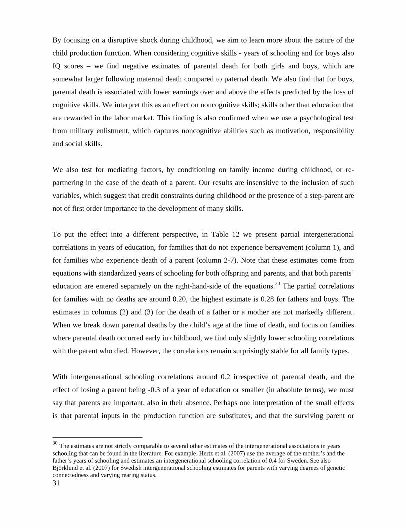
31

By focusing on a disruptive shock during childhood, we aim to learn more about the nature of the

child production function. When considering cognitive skills - years of schooling and for boys also

IQ scores – we find negative estimates of parental death for both girls and boys, which are

somewhat larger following maternal death compared to paternal death. We also find that for boys,

parental death is associated with lower earnings over and above the effects predicted by the loss of

cognitive skills. We interpret this as an effect on noncognitive skills; skills other than education that

are rewarded in the labor market. This finding is also confirmed when we use a psychological test

from military enlistment, which captures noncognitive abilities such as motivation, responsibility

and social skills.

We also test for mediating factors, by conditioning on family income during childhood, or re-

partnering in the case of the death of a parent. Our results are insensitive to the inclusion of such

variables, which suggest that credit constraints during childhood or the presence of a step-parent are

not of first order importance to the development of many skills.

To put the effect into a different perspective, in Table 12 we present partial intergenerational

correlations in years of education, for families that do not experience bereavement (column 1), and

for families who experience death of a parent (column 2-7). Note that these estimates come from

equations with standardized years of schooling for both offspring and parents, and that both parents’

education are entered separately on the right-hand-side of the equations.30 The partial correlations

for families with no deaths are around 0.20, the highest estimate is 0.28 for fathers and boys. The

estimates in columns (2) and (3) for the death of a father or a mother are not markedly different.

When we break down parental deaths by the child’s age at the time of death, and focus on families

where parental death occurred early in childhood, we find only slightly lower schooling correlations

with the parent who died. However, the correlations remain surprisingly stable for all family types.

With intergenerational schooling correlations around 0.2 irrespective of parental death, and the

effect of losing a parent being -0.3 of a year of education or smaller (in absolute terms), we must

say that parents are important, also in their absence. Perhaps one interpretation of the small effects

is that parental inputs in the production function are substitutes, and that the surviving parent or

30 The estimates are not strictly comparable to several other estimates of the intergenerational associations in years schooling that can be found in the literature. For example, Hertz et al. (2007) use the average of the mother’s and the father’s years of schooling and estimates an intergenerational schooling correlation of 0.4 for Sweden. See also Björklund et al. (2007) for Swedish intergenerational schooling estimates for parents with varying degrees of genetic connectedness and varying rearing status.

32

other family members (older siblings, grandparents) can compensate for the loss of a parent and

contribute to the skill formation of children. Genetics may also play a role here. The extended

family might be important as well. And maybe deceased parents also act as role models and pass on

expectations and aspirations given by their socio-economic status, education level and profession in

life. More research is needed to find out how important such mechanisms are.

33

References

Altonji, Joseph G. and Dunn, Thomas A. (1996), “The Effects of Family Characteristics on the Return to Education”, The Review of Economics and Statistics, 78(4), 692–704. Altonji, Joseph G., Elder, Todd E. and Taber, Christopher R. (2005) “Selection on Observed and Unobserved Variables: Assessing the Effectiveness of Catholic Schools”, Journal of Political Economy, 113(1), 151–184. Angrist, J.D., Krueger, A.B., (1991). Does compulsory school attendance affect schooling and earnings? Quarterly Journal of Economics 106, 979–1014. Angrist, J.D., Lavy, V., (1999). Using Maimonides’ rule to estimate the effect of class size on scholastic achievement. Quarterly Journal of Economics 114, 533–575. Amato, Paul R. (2010), “Research on Divorce: Continuing Trends and New Developments”, Journal of Marriage and Family, 72, 650-666. Amato, Paul. R., and Rivera, Fernando (1999), “Paternal involvement and children’s behavioral problems”. Journal of Marriage and the Family, 61, 375–384. Becker, Gary and Tomes, Nigel (1979), "An Equilibrium Theory of the Distribution of Income and Intergenerational Mobility", The Journal of Political Economy, 87(6), 1153–1189. Ben-Porath, Yoram (1967), “The production of human capital and the life cycle of earnings”, Journal of Political Economy, 75(4), 352–365. Bernal, Raquel. (2008), The Effect of Maternal Employment and Child Care on Children’s Cognitive Development” International Economic Review, 49, 1173–1209. Bernal, Raquel., and Keane, Michael P. (2010), “Quasi-Structural Estimation of a Model of Child Care Choices and Child Cognitive Production,” Journal of Econometrics, 156, 1, 164–189, Björklund, Anders and Sundström, Marianne (2006), ”Parental separation and children’s educational attainment: A sibling analysis on Swedish register data”, Economica, 73(292), 605–624. Björklund, Anders, Jäntti, Markus and Solon, Gary (2007), “Nature and Nurture in the Intergenerational Transmission of Socioeconomic Status: Evidence from Swedish Children and Their Biological and Rearing Parents”, The B.E. Journal of Economic Analysis & Policy, Vol. 7: Iss 2 (Advances), Article 4. Blau, Francine D. and Grossberg, Adam J. (1992), “Maternal Labor Supply and Children's Cognitive Development,” The Review of Economics and Statistics 74, 474–481. Butler, Jeffrey, Giuliano, Paula and Guiso, Luigi (2009), “The Right Amount of Trust.” NBER Working Paper 15344.

34

Carneiro, Pedro and Heckman James J. (2002), “The Evidence on Credit Constraints in Post-Secondary Schooling”, Economic Journal,112(482), 705–734. Caucutt, Elizabeth and Lochner, Lance J. (2004), “Early and Late Human Capital Investments, Credit Constraints, and the Family”, unpublished. Case, Anne and Ardington, Cally (2006), “The impact of parental death on school outcomes: Longitudinal evidence from South Africa”, Demography, 43(3), 401–420. Chen Stacey H., Chen, Yen-Chien and Liu, Jin-Tan (2009), “The Impact of Unexpected Maternal Death on Education: First Evidence from Three National Administrative Data Links.” American Economic Review 99(2), 149–153. Conner, D. B., Knight, D. K. and Cross, D. R. (1997). “Mothers’ and fathers’ scaffolding of their 2-year-olds during problem-solving and literacy interactions”, British Journal of Developmental Psychology, 15, 323–338. Corak, Miles (2001), “Death and Divorce: The Long-term Consequences of Parental Loss on Adolescents.” Journal of Labor Economics, 19(3), 682–715. Cunha, Flavio and Heckman, James J. (2007), "The Technology of Skill Formation." American Economic Review, 97(2), 31–47. Cunha, Flavio, and Heckman, James J. (2008), “Formulating, Identifying and Estimating the Technology of Cognitive and Noncognitive Skill Formation”, Journal of Human Resources 43(4), 738–782. Cunha, Flavio, Heckman James J. and Schennach, Susanne M. (2010), “Estimating the Technology of Cognitive and Noncognitive Skill Formation”, Econometrica 78(3), 883–931. Dustmann, Christian and Schönberg, Uta (2010) “Expansion in Maternity Leave Coverage, Early Maternal Employment and Children’s Long-Term Outcomes”, mimeo University College London. Erikson, Robert and Goldthorpe John H. (1992). The Constant Flux,. Oxford: Clarendon Press, 1992. Erikson, Robert and Torssander, Jenny (2008), “Social Class and Cause of Death,” European Journal of Public Health, 18(5), 473–478. Finansdepartementet (1986), “Socialbidrag.” Departementsstencil 1986:16. Francesconi, Marco, Jenkins, Stephen P. and Siedler, Thomas (2010), “Childhood family structure and schooling outcomes: evidence for Germany”, Journal of Population Economics 23(3), 1073–1103. Gertler, Paul, Levine, David I. and Ames, Minnie (2004), “Schooling and Parental Death”, The Review of Economics and Statistics, 86(1) 211–225. Hahn, Jinyong., Todd, Petra and Van Der Klaauw, Wilbert (2001),”Identification and estimation of treatment effects with a regression discontinuity design”, Econometrica 69, 201–209.

35

Haveman, Robert and Wolfe, Barbara (1995). “The Determinants of Children Attainments: A Review of Methods and Findings”, Journal of Economic Literature, 33(4), 1829–1878. Heckman, James J. and Rubinstein, Yona (2001) “The Importance of Noncognitive Skills: Lessons from the GED Testing Program”, American Economic Review, 91, 2, 145–149. Heckman, James J., Stixrud, Jora and Urzua, Sergio (2006), "The Effects of Cognitive and Noncognitive Abilities on Labor Market Outcomes and Social Behavior", Journal of Labor Economics 24(3), 411–482. Hertz, Tom, Jayasundera, Tamara, Piraino, Patrizio, Selcuk, Sibel, Smith, Nicole and Verashchagina, Alina (2007), “The Inheritance of Educational Inequality: International Comparisons and Fifty-Year Trends”, The B.E. Journal of Economic Analysis & Policy Vol. 7: Iss 2 (Advances), Article 10. Holmlund, Helena, Lindahl, Mikael and Plug, Erik (2011), “The Causal Effect of Parents’ Schooling on Children’s Schooling: A Comparison of Estimation Methods.” Journal of Economic Literature forthcoming. Kjellberg, Anders (2009), “Det fackliga medlemsraset i Sverige under 2007 och 2008,” Arbetsmarknad & Arbetsliv 15(2), 11–28. Koestner, Richard., Franz, Carol. and Weinberger, Joel (1990). “The family origins of empathetic concern: A twenty-six year longitudinal study”, Journal of Personality and Social Psychology 58 (4) 709-717. Lang Kevin and Zagorsky Jay L. (2001), “Does Growing up with a Parent Absent Really Hurt?”, The Journal of Human Resources, 36(2), 253–273. Liebowitz, Arleen (1974), “Home investments in children”, Journal of Political Economy, 82(2), S111–S131. Lindquist, Matthew and Sjögren Lindquist, Gabriella (2011), ”The dynamics of child poverty in Sweden.” Journal of Population Economics, forthcoming. Lindqvist, Erik and Vestman, Roine (2011). “The Labor Market Returns to Cognitive and Noncognitive Ability: Evidence from the Swedish Enlistment.” American Economic Journal: Applied Economics, 3, 101–128. Liu, Qian and Nordström Skans, Oskar (2010) "The Duration of Paid Parental Leave and Children's Scholastic Performance," The B.E. Journal of Economic Analysis & Policy: Vol. 10 : Iss. 1 (Contributions), Article 3. McLanahan, Sara (2004). “Diverging Destinies: How Children Fare Under the Second Demographic Transition.” Demography 41(4), 607–627. Parcel, Toby L. and Menaghan, Elizabeth G. (1994), “Early parental work, family social capital and early childhood outcomes”, American Journal of Sociology 99(4), 972–1009. Rosenzweig, Mark R. and Wolpin, Kenneth I. (1994), “Are there increasing returns to the Intergenerational production of human capital? Maternal schooling and child intellectual

36

achievement.” The Journal of Human Resources, 29(2), 670–693. Ståhlberg, Ann-Charlotte (2006), “An international comparison of survivors’ pensions. The case of Sweden”, Conseil d’orientation des retraites (COR), Paris. OECD. Todd, Petra E. and Wolpin, Kenneth I. (2003), “On the Specification and Estimation of the Production Function for Cognitive Achievement.” Economic Journal, 113(485), F3–F33. Todd Petra and Wolpin, Kenneth I. (2007) “The Production of Cognitive Achievement in Children: Home, School and Racial Test Score Gaps”, Journal of Human Capital, 1, 91-136.  Tulving, Endel (1983), Elements of episodic memory, Oxford: Oxford University Press. Wickens, Michael R. (1972) “A Note on the Use of Proxy Variables”, Econometrica, 40(4), 759–

761.

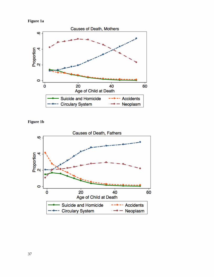
37

Figure 1a

Figure 1b

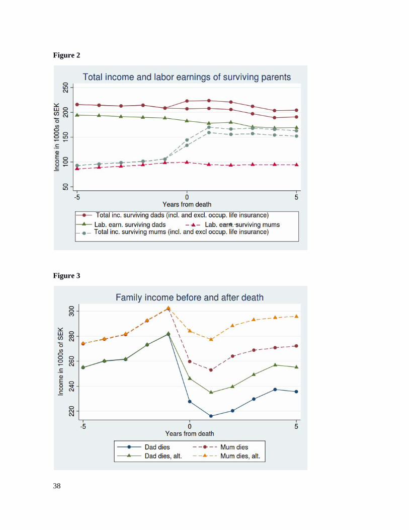
38

Figure 2

Figure 3

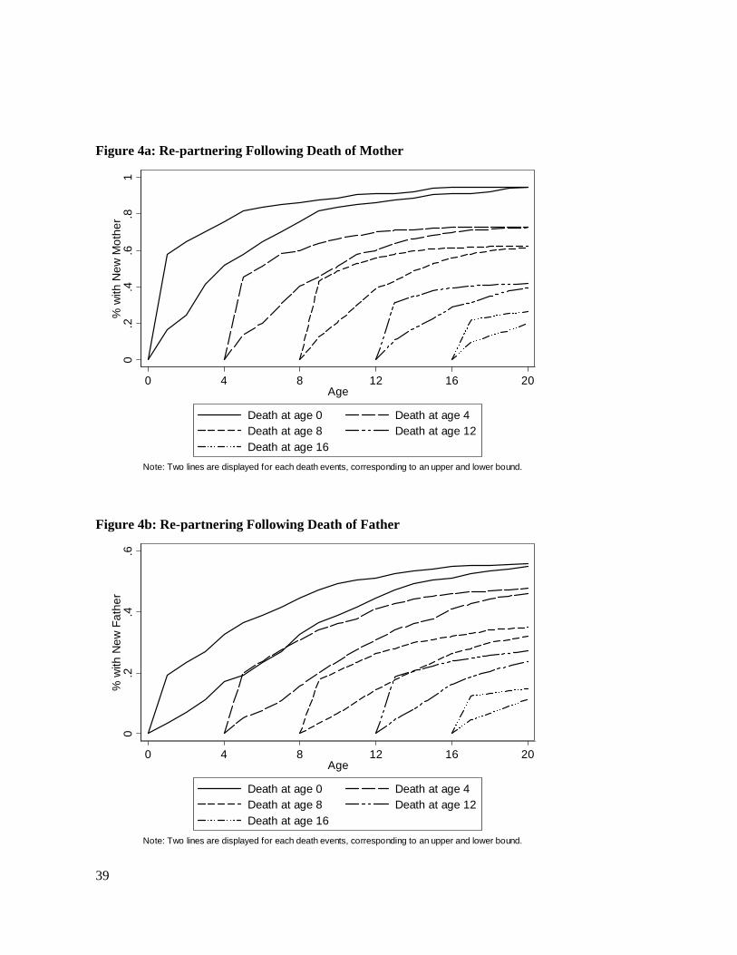
39

Figure 4a: Re-partnering Following Death of Mother

Figure 4b: Re-partnering Following Death of Father

0.2

.4.6

.81

% w

ith N

ew

Mo

the

r

0 4 8 12 16 20Age

Death at age 0 Death at age 4Death at age 8 Death at age 12

Death at age 16

Note: Two lines are displayed for each death events, corresponding to an upper and lower bound.

0.2

.4.6

% w

ith N

ew

Fa

the

r

0 4 8 12 16 20Age

Death at age 0 Death at age 4Death at age 8 Death at age 12

Death at age 16

Note: Two lines are displayed for each death events, corresponding to an upper and lower bound.

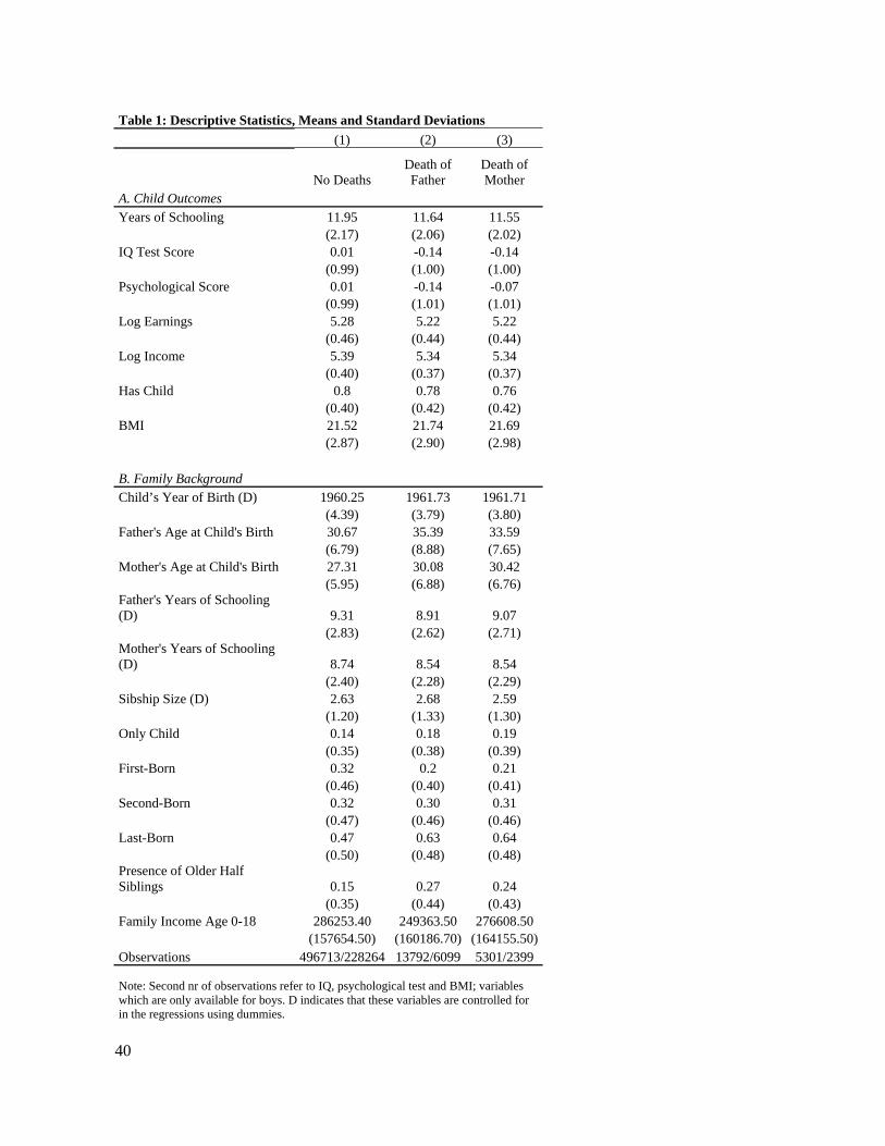
40

Table 1: Descriptive Statistics, Means and Standard Deviations

(1) (2) (3)

No Deaths Death of Father

Death of Mother

A. Child Outcomes Years of Schooling 11.95 11.64 11.55 (2.17) (2.06) (2.02) IQ Test Score 0.01 -0.14 -0.14 (0.99) (1.00) (1.00) Psychological Score 0.01 -0.14 -0.07 (0.99) (1.01) (1.01) Log Earnings 5.28 5.22 5.22 (0.46) (0.44) (0.44) Log Income 5.39 5.34 5.34 (0.40) (0.37) (0.37) Has Child 0.8 0.78 0.76 (0.40) (0.42) (0.42) BMI 21.52 21.74 21.69 (2.87) (2.90) (2.98) B. Family Background Child’s Year of Birth (D) 1960.25 1961.73 1961.71 (4.39) (3.79) (3.80) Father's Age at Child's Birth 30.67 35.39 33.59 (6.79) (8.88) (7.65) Mother's Age at Child's Birth 27.31 30.08 30.42 (5.95) (6.88) (6.76) Father's Years of Schooling (D) 9.31 8.91 9.07 (2.83) (2.62) (2.71) Mother's Years of Schooling (D) 8.74 8.54 8.54 (2.40) (2.28) (2.29) Sibship Size (D) 2.63 2.68 2.59 (1.20) (1.33) (1.30) Only Child 0.14 0.18 0.19 (0.35) (0.38) (0.39) First-Born 0.32 0.2 0.21 (0.46) (0.40) (0.41)Second-Born 0.32 0.30 0.31 (0.47) (0.46) (0.46)Last-Born 0.47 0.63 0.64 (0.50) (0.48) (0.48) Presence of Older Half Siblings 0.15 0.27 0.24 (0.35) (0.44) (0.43) Family Income Age 0-18 286253.40 249363.50 276608.50 (157654.50) (160186.70) (164155.50)Observations 496713/228264 13792/6099 5301/2399

Note: Second nr of observations refer to IQ, psychological test and BMI; variables which are only available for boys. D indicates that these variables are controlled for in the regressions using dummies.

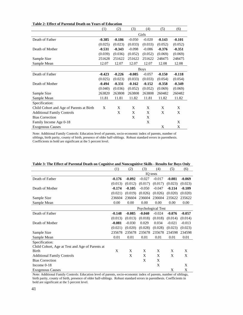
41

Table 2: Effect of Parental Death on Years of Education (1) (2) (3) (4) (5) (6) Girls Death of Father -0.385 -0.186 -0.050 -0.020 -0.143 -0.101 (0.025) (0.023) (0.033) (0.033) (0.052) (0.052) Death of Mother -0.531 -0.343 -0.098 -0.086 -0.376 -0.351 (0.039) (0.036) (0.052) (0.052) (0.069) (0.069) Sample Size 251628 251622 251622 251622 248475 248475 Sample Mean 12.07 12.07 12.07 12.07 12.08 12.08 Boys Death of Father -0.423 -0.226 -0.085 -0.057 -0.150 -0.118 (0.025) (0.023) (0.033) (0.033) (0.054) (0.054) Death of Mother -0.494 -0.331 -0.162 -0.152 -0.358 -0.349 (0.040) (0.036) (0.052) (0.052) (0.069) (0.069) Sample Size 263820 263808 263808 263808 260482 260482 Sample Mean 11.81 11.81 11.82 11.81 11.82 11.82 Specification: Child Cohort and Age of Parents at Birth X X X X X X Additional Family Controls X X X X X Bias Correction X X Family Income Age 0-18 X X Exogenous Causes X X

Note: Additional Family Controls: Education level of parents, socio-economic index of parents, number of siblings, birth parity, county of birth, presence of older half-siblings. Robust standard errors in parenthesis. Coefficients in bold are significant at the 5 percent level.

Table 3: The Effect of Parental Death on Cognitive and Noncognitive Skills - Results for Boys Only (1) (2) (3) (4) (5) (6) IQ tests Death of Father -0.176 -0.092 -0.027 -0.017 -0.081 -0.069 (0.013) (0.012) (0.017) (0.017) (0.023) (0.023) Death of Mother -0.174 -0.105 -0.050 -0.047 -0.114 -0.109 (0.021) (0.019) (0.026) (0.026) (0.020) (0.020) Sample Size 236604 236604 236604 236604 235622 235622 Sample Mean 0.00 0.00 0.00 0.00 0.00 0.00 Psychological Test Death of Father -0.148 -0.085 -0.040 -0.024 -0.076 -0.057 (0.013) (0.013) (0.018) (0.018) (0.014) (0.014) Death of Mother -0.081 -0.030 0.029 0.034 -0.021 -0.013 (0.021) (0.020) (0.028) (0.028) (0.023) (0.023) Sample Size 235678 235678 235678 235678 234598 234598 Sample Mean 0.01 0.01 0.01 0.01 0.01 0.01 Specification: Child Cohort, Age at Test and Age of Parents at Birth X X X X X X Additional Family Controls X X X X X Bias Correction X X Income 0-18 X X Exogenous Causes X X Note: Additional Family Controls: Education level of parents, socio-economic index of parents, number of siblings, birth parity, county of birth, presence of older half-siblings. Robust standard errors in parenthesis. Coefficients in bold are significant at the 5 percent level.

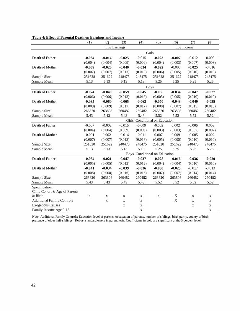
42

Table 4: Effect of Parental Death on Earnings and Income (1) (2) (3) (4) (5) (6) (7) (8) Log Earnings Log Income Girls Death of Father -0.034 -0.014 -0.025 -0.015 -0.023 -0.007 -0.012 0.003 (0.004) (0.004) (0.009) (0.009) (0.004) (0.003) (0.007) (0.008)Death of Mother -0.039 -0.020 -0.040 -0.034 -0.022 -0.008 -0.025 -0.016 (0.007) (0.007) (0.013) (0.013) (0.006) (0.005) (0.010) (0.010)Sample Size 251628 251622 248475 248475 251628 251622 248475 248475 Sample Mean 5.13 5.13 5.13 5.13 5.25 5.25 5.25 5.25 Boys Death of Father -0.074 -0.040 -0.059 -0.045 -0.065 -0.034 -0.047 -0.027 (0.006) (0.006) (0.013) (0.013) (0.005) (0.005) (0.010) (0.010) Death of Mother -0.085 -0.060 -0.065 -0.062 -0.070 -0.048 -0.040 -0.035 (0.009) (0.009) (0.017) (0.017) (0.008) (0.007) (0.015) (0.015) Sample Size 263820 263808 260482 260482 263820 263808 260482 260482 Sample Mean 5.43 5.43 5.43 5.43 5.52 5.52 5.52 5.52 Girls, Conditional on Education Death of Father -0.007 -0.002 -0.015 -0.009 -0.002 0.002 -0.005 0.008 (0.004) (0.004) (0.009) (0.009) (0.003) (0.003) (0.007) (0.007) Death of Mother -0.001 0.002 -0.014 -0.011 0.007 0.009 -0.005 0.002 (0.007) (0.007) (0.013) (0.013) (0.005) (0.005) (0.010) (0.010) Sample Size 251628 251622 248475 248475 251628 251622 248475 248475 Sample Mean 5.13 5.13 5.13 5.13 5.25 5.25 5.25 5.25 Boys, Conditional on Education Death of Father -0.034 -0.021 -0.047 -0.037 -0.028 -0.016 -0.036 -0.020 (0.005) (0.005) (0.012) (0.012) (0.004) (0.004) (0.010) (0.010) Death of Mother -0.041 -0.034 -0.039 -0.036 -0.030 -0.025 -0.017 -0.013 (0.008) (0.008) (0.016) (0.016) (0.007) (0.007) (0.014) (0.014) Sample Size 263820 263808 260482 260482 263820 263808 260482 260482 Sample Mean 5.43 5.43 5.43 5.43 5.52 5.52 5.52 5.52 Specification: Child Cohort & Age of Parents at Birth x x x x x X x x Additional Family Controls x x x X x x Exogenous Causes x x x x Family Income Age 0-18 x x

Note: Additional Family Controls: Education level of parents, occupation of parents, number of siblings, birth parity, county of birth, presence of older half-siblings. Robust standard errors in parenthesis. Coefficients in bold are significant at the 5 percent level.

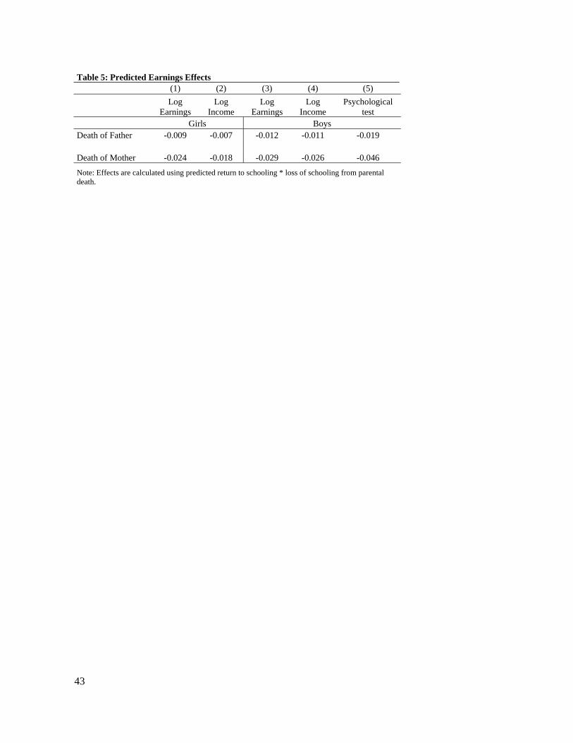
43

Table 5: Predicted Earnings Effects (1) (2) (3) (4) (5)

Log

Earnings Log

IncomeLog

EarningsLog

IncomePsychological

test Girls BoysDeath of Father -0.009 -0.007 -0.012 -0.011 -0.019 Death of Mother -0.024 -0.018 -0.029 -0.026 -0.046

Note: Effects are calculated using predicted return to schooling * loss of schooling from parental death.

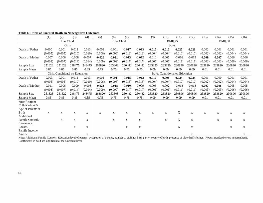
44

Table 6: Effect of Parental Death on Noncognitive Outcomes (1) (2) (3) (4) (5) (6) (7) (8) (9) (10) (11) (12) (13) (14) (15) (16) Has Child Has Child BMI≥25 BMI≥30 Girls Boys Death of Father 0.000 -0.001 0.012 0.013 -0.003 -0.001 -0.017 -0.013 0.015 0.010 0.025 0.026 0.002 0.001 0.001 0.001 (0.005) (0.005) (0.010) (0.010) (0.006) (0.006) (0.013) (0.013) (0.004) (0.004) (0.010) (0.010) (0.002) (0.002) (0.004) (0.004) Death of Mother -0.007 -0.006 -0.008 -0.007 -0.026 -0.021 -0.013 -0.012 0.010 0.005 -0.016 -0.015 0.009 0.007 0.006 0.006 (0.008) (0.007) (0.014) (0.014) (0.009) (0.009) (0.017) (0.017) (0.006) (0.006) (0.011) (0.011) (0.003) (0.003) (0.006) (0.006) Sample Size 251628 251622 248475 248475 263820 263808 260482 260482 233820 233820 230896 230896 233820 233820 230896 230896 Sample Mean 0.85 0.85 0.85 0.85 0.75 0.75 0.75 0.75 0.09 0.09 0.09 0.09 0.01 0.01 0.01 0.01 Girls, Conditional on Education Boys, Conditional on Education Death of Father -0.003 -0.001 0.011 0.013 -0.001 0.001 -0.015 -0.012 0.010 0.008 0.024 0.025 0.001 0.000 0.001 0.001 (0.005) (0.005) (0.010) (0.010) (0.006) (0.006) (0.013) (0.013) (0.004) (0.004) (0.010) (0.010) (0.002) (0.002) (0.004) (0.004) Death of Mother -0.011 -0.008 -0.009 -0.008 -0.023 -0.018 -0.010 -0.009 0.005 0.002 -0.018 -0.018 0.007 0.006 0.005 0.005 (0.008) (0.007) (0.014) (0.014) (0.009) (0.009) (0.017) (0.017) (0.006) (0.006) (0.011) (0.011) (0.003) (0.003) (0.006) (0.006) Sample Size 251628 251622 248475 248475 263820 263808 260482 260482 233820 233820 230896 230896 233820 233820 230896 230896 Sample Mean 0.85 0.85 0.85 0.85 0.75 0.75 0.75 0.75 0.09 0.09 0.09 0.09 0.01 0.01 0.01 0.01 Specification: Child Cohort & Age of Parents at Birth x x x x x x x x x x X x x x x x Additional Family Controls x x x x x x x X x x x x Exogenous Causes x x x x X x x x Family Income Age 0-18 x x x x Note: Additional Family Controls: Education level of parents, occupation of parents, number of siblings, birth parity, county of birth, presence of older half-siblings. Robust standard errors in parenthesis. Coefficients in bold are significant at the 5 percent level.

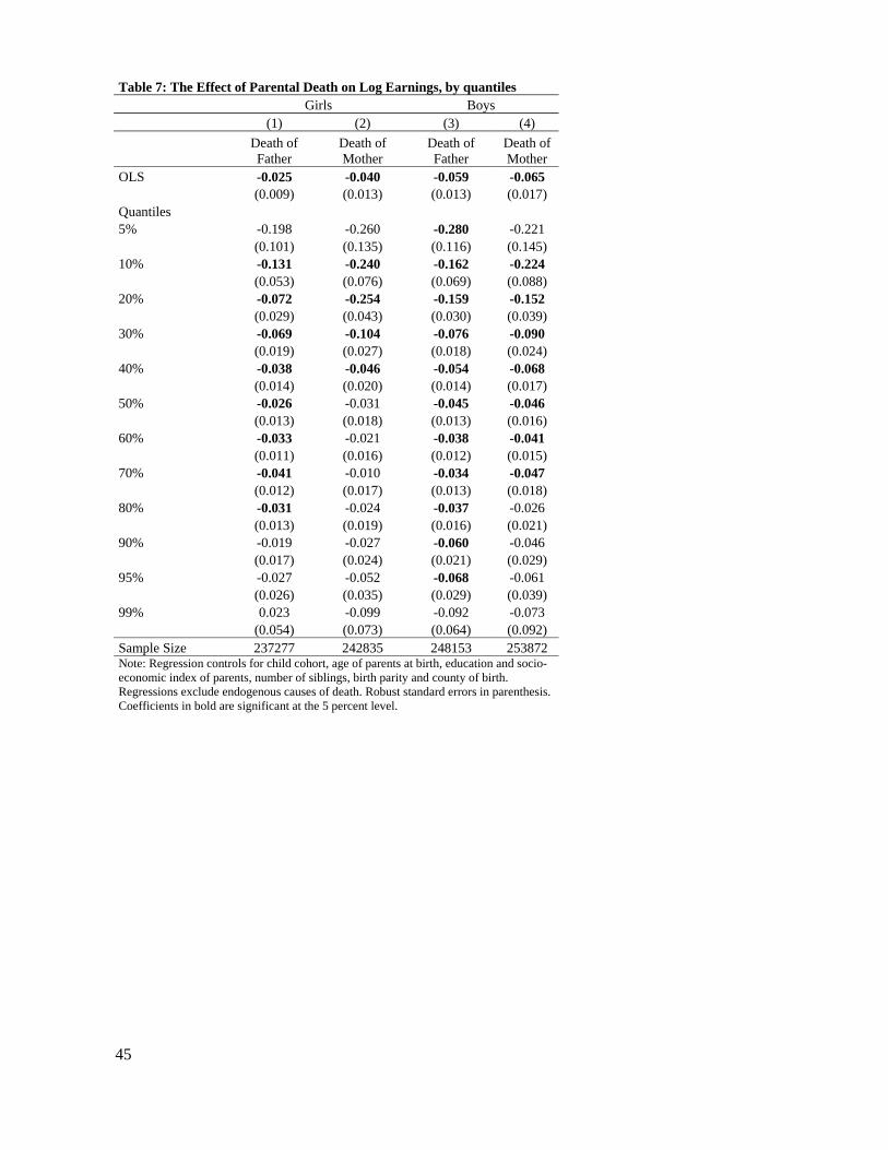
45

Table 7: The Effect of Parental Death on Log Earnings, by quantiles Girls Boys (1) (2) (3) (4)

Death of Father

Death of Mother

Death of Father

Death of Mother

OLS -0.025 -0.040 -0.059 -0.065 (0.009) (0.013) (0.013) (0.017) Quantiles 5% -0.198 -0.260 -0.280 -0.221 (0.101) (0.135) (0.116) (0.145)10% -0.131 -0.240 -0.162 -0.224 (0.053) (0.076) (0.069) (0.088)20% -0.072 -0.254 -0.159 -0.152 (0.029) (0.043) (0.030) (0.039) 30% -0.069 -0.104 -0.076 -0.090 (0.019) (0.027) (0.018) (0.024) 40% -0.038 -0.046 -0.054 -0.068 (0.014) (0.020) (0.014) (0.017) 50% -0.026 -0.031 -0.045 -0.046 (0.013) (0.018) (0.013) (0.016) 60% -0.033 -0.021 -0.038 -0.041 (0.011) (0.016) (0.012) (0.015) 70% -0.041 -0.010 -0.034 -0.047 (0.012) (0.017) (0.013) (0.018)80% -0.031 -0.024 -0.037 -0.026 (0.013) (0.019) (0.016) (0.021)90% -0.019 -0.027 -0.060 -0.046 (0.017) (0.024) (0.021) (0.029) 95% -0.027 -0.052 -0.068 -0.061 (0.026) (0.035) (0.029) (0.039) 99% 0.023 -0.099 -0.092 -0.073 (0.054) (0.073) (0.064) (0.092) Sample Size 237277 242835 248153 253872 Note: Regression controls for child cohort, age of parents at birth, education and socio-economic index of parents, number of siblings, birth parity and county of birth. Regressions exclude endogenous causes of death. Robust standard errors in parenthesis. Coefficients in bold are significant at the 5 percent level.

46

Table 8: The Effect of Parental Death on Log Income, by quantiles Girls Boys (1) (2) (3) (4)

Death of Father

Death of Mother

Death of Father

Death of Mother

OLS -0.012 -0.025 -0.047 -0.040 (0.007) (0.010) (0.010) (0.015) Quantiles 5% -0.081 -0.014 -0.089 -0.138 (0.050) (0.070) (0.066) (0.086) 10% -0.025 -0.111 -0.105 -0.131 (0.034) (0.046) (0.040) (0.051) 20% -0.022 -0.040 -0.073 -0.075 (0.017) (0.023) (0.020) (0.026) 30% -0.016 -0.031 -0.041 -0.074 (0.013) (0.018) (0.013) (0.017) 40% -0.019 -0.028 -0.050 -0.049 (0.010) (0.014) (0.012) (0.014) 50% -0.025 -0.025 -0.045 -0.043 (0.010) (0.014) (0.012) (0.015) 60% -0.021 -0.015 -0.038 -0.037 (0.010) (0.014) (0.012) (0.015) 70% -0.021 -0.020 -0.038 -0.050 (0.010) (0.015) (0.013) (0.017) 80% -0.014 -0.012 -0.036 -0.038 (0.014) (0.018) (0.016) (0.021) 90% -0.024 -0.017 -0.047 -0.052 (0.018) (0.026) (0.023) (0.030) 95% -0.008 -0.044 -0.073 -0.007 (0.025) (0.033) (0.031) (0.041) 99% -0.021 -0.095 -0.160 0.088 (0.061) (0.086) (0.091) (0.125) Sample Size 242076 247780 253675 259553 Note: Regression controls for child cohort, age of parents at birth, education and socio-economic index of parents, number of siblings, birth parity and county of birth. Regressions exclude endogenous causes of death. Robust standard errors in parenthesis. Coefficients in bold are significant at the 5 percent level.

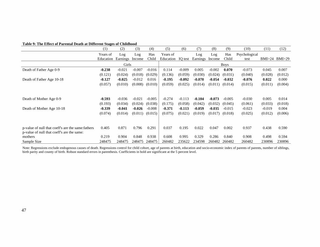
47

Table 9: The Effect of Parental Death at Different Stages of Childhood (1) (2) (3) (4) (5) (6) (7) (8) (9) (10) (11) (12)

Years of

EducationLog

EarningsLog

IncomeHas

ChildYears of

Education IQ test Log

EarningsLog

IncomeHas

ChildPsychological

test BMI>24 BMI>29 Girls Boys Death of Father Age 0-9 -0.238 -0.021 -0.007 -0.016 0.114 -0.009 0.005 -0.002 0.070 -0.073 0.045 0.007 (0.121) (0.024) (0.018) (0.029) (0.136) (0.059) (0.030) (0.024) (0.031) (0.040) (0.028) (0.012) Death of Father Age 10-18 -0.127 -0.025 -0.012 0.016 -0.195 -0.092 -0.070 -0.054 -0.032 -0.076 0.022 0.000 (0.057) (0.010) (0.008) (0.010) (0.059) (0.025) (0.014) (0.011) (0.014) (0.015) (0.011) (0.004) Death of Mother Age 0-9 -0.593 -0.036 -0.021 -0.005 -0.274 -0.113 -0.104 -0.073 -0.005 -0.030 0.005 0.014 (0.193) (0.034) (0.024) (0.038) (0.175) (0.058) (0.042) (0.032) (0.045) (0.061) (0.033) (0.018) Death of Mother Age 10-18 -0.339 -0.041 -0.026 -0.008 -0.371 -0.113 -0.059 -0.035 -0.015 -0.023 -0.019 0.004 (0.074) (0.014) (0.011) (0.015) (0.075) (0.021) (0.019) (0.017) (0.018) (0.025) (0.012) (0.006) p-value of null that coeff's are the same:fathers 0.405 0.871 0.796 0.291 0.037 0.195 0.022 0.047 0.002 0.937 0.438 0.590 p-value of null that coeff's are the same: mothers 0.219 0.904 0.848 0.938 0.608 0.995 0.329 0.286 0.840 0.908 0.498 0.594 Sample Size 248475 248475 248475 248475 260482 235622 234598 260482 260482 260482 230896 230896

Note: Regressions exclude endogenous causes of death. Regressions control for child cohort, age of parents at birth, education and socio-economic index of parents of parents, number of siblings, birth parity and county of birth. Robust standard errors in parenthesis. Coefficients in bold are significant at the 5 percent level.

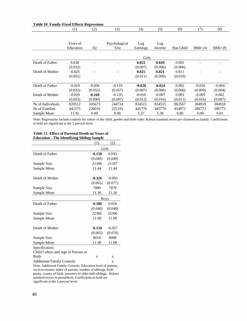
48

Table 10: Family-Fixed Effects Regressions (1) (2) (3) (4) (5) (6) (7) (8)

Years of

Education IQ Psychological

Test Log

Earnings Log

Income Has Child BMI>24 BMI>29

Girls Death of Father 0.038 - - 0.023 0.020 0.001 - - (0.032) (0.007) (0.006) (0.006) Death of Mother -0.025 - - 0.025 0.021 0.011 - - (0.051) (0.011) (0.009) (0.010) Death of Father -0.019 -0.056 -0.110 -0.028 -0.024 0.002 -0.010 -0.004 (0.032) (0.055) (0.057) (0.007) (0.006) (0.006) (0.009) (0.004) Death of Mother -0.029 -0.169 -0.135 -0.010 -0.007 0.003 -0.005 0.002 (0.053) (0.090) (0.097) (0.012) (0.010) (0.011) (0.016) (0.007) Nr of Individuals 820512 245673 244724 834515 834515 863567 384918 384918 Nr of Families 442375 226016 225191 445776 445776 454973 286773 286773 Sample Mean 11.91 0.00 0.00 5.27 5.38 0.86 0.09 0.01 Note: Regressions include controls for cohort of the child, gender and birth order. Robust standard errors are clustered on family. Coefficients in bold are significant at the 5 percent level.

Table 11: Effect of Parental Death on Years of Education - The Identifying Sibling Sample (1) (2) Girls Death of Father -0.158 0.045 (0.040) (0.049) Sample Size 21348 21347 Sample Mean 11.44 11.44 Death of Mother -0.326 -0.093 (0.065) (0.077) Sample Size 7880 7879 Sample Mean 11.36 11.36 Boys Death of Father -0.180 0.056 (0.040) (0.048)Sample Size 22306 22306 Sample Mean 11.08 11.08 Death of Mother -0.134 -0.057 (0.065) (0.079) Sample Size 8010 8008 Sample Mean 11.08 11.08 Specification: Child Cohort and Age of Parents at Birth x x Additional Family Controls x Note: Additional Family Controls: Education level of parents, socio-economic index of parents, number of siblings, birth parity, county of birth, presence of older half-siblings. Robust standard errors in parenthesis. Coefficients in bold are significant at the 5 percent level.

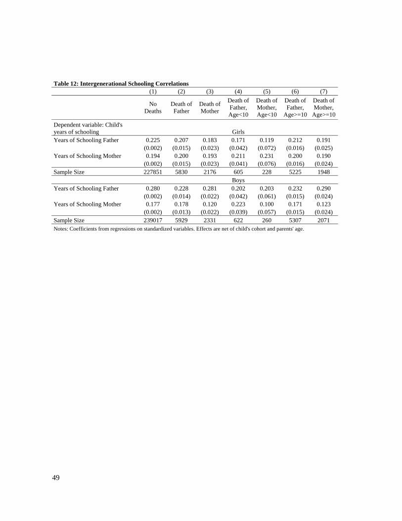
49

Table 12: Intergenerational Schooling Correlations (1) (2) (3) (4) (5) (6) (7)

No Deaths

Death of Father

Death of Mother

Death of Father, Age<10

Death of Mother, Age<10

Death of Father,

Age>=10

Death of Mother,

Age>=10Dependent variable: Child's years of schooling Girls Years of Schooling Father 0.225 0.207 0.183 0.171 0.119 0.212 0.191 (0.002) (0.015) (0.023) (0.042) (0.072) (0.016) (0.025) Years of Schooling Mother 0.194 0.200 0.193 0.211 0.231 0.200 0.190 (0.002) (0.015) (0.023) (0.041) (0.076) (0.016) (0.024) Sample Size 227851 5830 2176 605 228 5225 1948 Boys Years of Schooling Father 0.280 0.228 0.281 0.202 0.203 0.232 0.290 (0.002) (0.014) (0.022) (0.042) (0.061) (0.015) (0.024) Years of Schooling Mother 0.177 0.178 0.120 0.223 0.100 0.171 0.123 (0.002) (0.013) (0.022) (0.039) (0.057) (0.015) (0.024) Sample Size 239017 5929 2331 622 260 5307 2071 Notes: Coefficients from regressions on standardized variables. Effects are net of child's cohort and parents' age.

50

Appendix A.

A.1 Derivation of the Unbiased Estimator

Consider the model

where we have suppressed the constant and a set of explanatory variables X for ease of exposition.

If a constant or explanatory variables are needed, one can project S, D and P on these. We assume

that the true value of β is zero, as the event S precedes the event P.

Suppose we regress S on D and P. These (biased) OLS coefficients are expressed as:

, , ,,

and

, , ,,

Express the covariance between the auxiliary variable and the error term as:

, ,

where μ is the ratio of the correlations as defined in (4). Replacing cov(P,u) above gives:

,

,, ,

Hence an unbiased estimator of α is:

, ,

A.2 Monte Carlo assessment of our estimator in equation (7)

We perform Monte Carlo simulation to assess the property of our estimator. We simulate data based

on equation (3), using coefficients which are of the same magnitude with what we find in the

empirical section of the paper. The effect of parental death on years of education (the true value of

the coefficient) is set at -0.1 years. The variance of the residual is set to 2, which is close to the

variance of the OLS residual. We vary the correlation between parental death and unobserved

characteristics, between -0.16 to -0.04. A higher correlation in absolute level implies a greater

endogeneity of parental death. We set the proportion of parental death to 3 percent, which is close

to the proportion we see in the real data. We set the sample sizes to 100,000 and 1,000.

51

The results are displayed in Table A1. The first panel reports the results for a large sample. The

table first reports the average of the OLS estimate and its standard deviation. Not surprisingly, the

more important the endogeneity, the greater the bias. We next display the average bias-corrected

estimates using our proposed method. As expected, the average is very close to the true value.

However, the standard deviation is higher than in the OLS case. Finally, we report the percentage of

cases where the true value belongs to the 95 percent confidence interval of our estimator. When

working with a much smaller sample, the OLS coefficients are biased in a similar way, with larger

standard deviations. Our estimator performs more poorly and tends to over-estimate the true value

and its standard deviation can be quite large.

Table A1: Monte Carlo Results

Corr(D,u) -0.16 -0.10 -0.07 -0.04 Sample Size=100,000

OLS Mean -2.32 -2.17 -1.48 -0.65 St. Dev. 0.037 0.053 0.058 0.042 Bias Corrected Mean -0.0999 -0.0952 -0.102 -0.0996 St. Dev. 0.064 0.090 0.087 0.059

% cases where true value belongs to 95% confidence interval 93.1% 93.1% 93.2% 96.2%

Sample Size=1,000 OLS Mean -2.31 -2.15 -1.47 -0.65 St. Dev. 0.39 0.57 0.60 0.45 Bias Corrected Mean -0.076 0.078 0.001 -0.081 St. Dev. 0.673 1.027 0.914 0.660

% cases where true value belongs to 95% confidence interval 92.7% 92.6% 94.7% 94.7%

Note: All results based on 1000 Monte Carlo replications. True value = -0.1 Appendix Table B1: Test for Exogeneity of Causes of Death Dependent Variable: Years of Education

Cause Auxiliary

Coeff. Standard

Error t-

value Auxiliary

Coeff. Standard

Error t-value Death of Father Death of Mother Infectious and Parasitic Disease -0.25 0.15 -1.65 -0.19 0.27 -0.73 Neoplasm -0.21 0.04 -4.80 -0.15 0.05 -3.00 Endocrine and Metabolic Diseases -0.02 0.16 -0.14 -0.05 0.21 -0.25 Mental and Behavioural Disorder -0.28 0.13 -2.18 -0.33 0.27 -1.24 Circulatory System -0.18 0.03 -5.41 -0.57 0.07 -7.88 Respiratory System -0.25 0.11 -2.30 -0.44 0.18 -2.41 Digestive System -0.21 0.09 -2.22 -0.54 0.15 -3.60 Other 0.03 0.22 0.14 -0.36 0.31 -1.17 Accidents -0.01 0.08 -0.14 -0.10 0.14 -0.73 Suicide and Homicide -0.21 0.10 -2.10 -0.13 0.16 -0.85

Note: Each coefficient is from a separate regression including as independent variables parental death at age 0-18 and the auxiliary variable defined as parental death at age 23-24. Regressions control for child cohort, age of parents at birth, education and socio-economic index of parents, number of siblings, birth parity and county of birth. We define exogenous causes as those with a t-value<1.64.

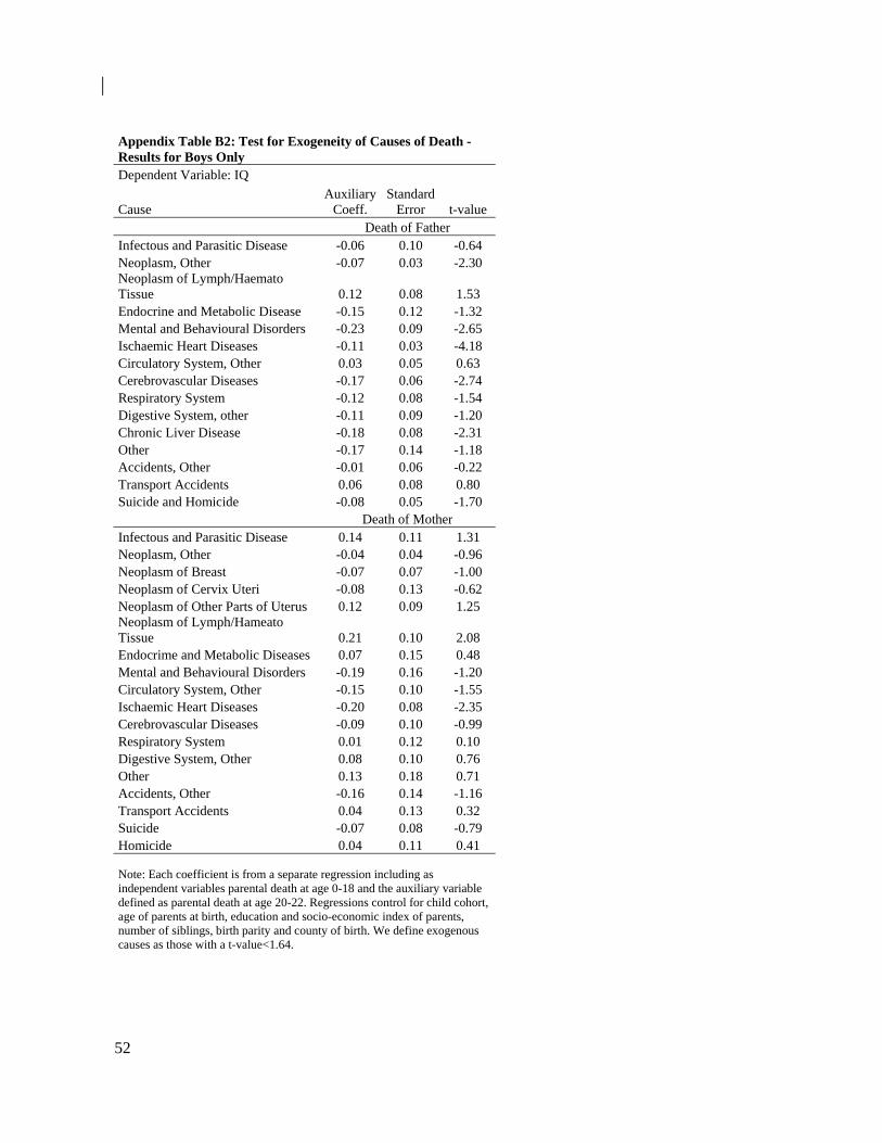
52

Appendix Table B2: Test for Exogeneity of Causes of Death - Results for Boys Only Dependent Variable: IQ

Cause Auxiliary

Coeff. Standard

Error t-value Death of Father Infectous and Parasitic Disease -0.06 0.10 -0.64 Neoplasm, Other -0.07 0.03 -2.30 Neoplasm of Lymph/Haemato Tissue 0.12 0.08 1.53 Endocrine and Metabolic Disease -0.15 0.12 -1.32Mental and Behavioural Disorders -0.23 0.09 -2.65 Ischaemic Heart Diseases -0.11 0.03 -4.18 Circulatory System, Other 0.03 0.05 0.63 Cerebrovascular Diseases -0.17 0.06 -2.74 Respiratory System -0.12 0.08 -1.54 Digestive System, other -0.11 0.09 -1.20 Chronic Liver Disease -0.18 0.08 -2.31 Other -0.17 0.14 -1.18 Accidents, Other -0.01 0.06 -0.22 Transport Accidents 0.06 0.08 0.80 Suicide and Homicide -0.08 0.05 -1.70 Death of MotherInfectous and Parasitic Disease 0.14 0.11 1.31Neoplasm, Other -0.04 0.04 -0.96 Neoplasm of Breast -0.07 0.07 -1.00 Neoplasm of Cervix Uteri -0.08 0.13 -0.62 Neoplasm of Other Parts of Uterus 0.12 0.09 1.25 Neoplasm of Lymph/Hameato Tissue 0.21 0.10 2.08 Endocrime and Metabolic Diseases 0.07 0.15 0.48 Mental and Behavioural Disorders -0.19 0.16 -1.20 Circulatory System, Other -0.15 0.10 -1.55 Ischaemic Heart Diseases -0.20 0.08 -2.35 Cerebrovascular Diseases -0.09 0.10 -0.99 Respiratory System 0.01 0.12 0.10 Digestive System, Other 0.08 0.10 0.76 Other 0.13 0.18 0.71 Accidents, Other -0.16 0.14 -1.16 Transport Accidents 0.04 0.13 0.32 Suicide -0.07 0.08 -0.79 Homicide 0.04 0.11 0.41

Note: Each coefficient is from a separate regression including as independent variables parental death at age 0-18 and the auxiliary variable defined as parental death at age 20-22. Regressions control for child cohort, age of parents at birth, education and socio-economic index of parents, number of siblings, birth parity and county of birth. We define exogenous causes as those with a t-value<1.64.

53

Appendix Table B3: Test for Exogeneity of Causes of Death - Results for Boys only Dependent Variable: Psychological Test

Cause Auxiliary

coeff. Standard

error t-value Auxiliary

coeff. Standard

error t-value Death of Father Death of Mother Infectious and Parasitic Disease 0.13 0.10 1.26 -0.14 0.12 -1.19 Neoplasm 0.02 0.03 0.57 -0.06 0.04 -1.62 Endocrine and Metabolic Diseases 0.14 0.12 1.18 -0.02 0.15 -0.14 Mental and Behavioural Disorder -0.10 0.10 -1.06 -0.06 0.18 -0.35 Circulatory System -0.03 0.02 -1.21 -0.10 0.06 -1.81 Respiratory System -0.17 0.08 -2.14 -0.14 0.13 -1.14 Digestive System -0.13 0.06 -2.13 -0.02 0.09 -0.25 Other -0.11 0.17 -0.69 0.00 0.19 0.02 Accidents -0.06 0.05 -1.28 -0.24 0.09 -2.75 Suicide and Homicide -0.10 0.06 -1.65 -0.13 0.10 -1.39

Note: Each coefficient is from a separate regression including as independent variables parental death at age 0-18 and the auxiliary variable defined as parental death at age 20-22. Regressions control for child cohort, age of parents at birth, education and socio-economic index of parents, number of siblings, birth parity and county of birth. We define exogenous causes as those with a t-value<1.64.

Appendix Table B4: Test of Significance of Auxiliary Variable for All Exogenous Causes of Death: t-statistics

Girls Boys

Years of

Education Exogenous Causes Death of Father -0.32 0.15 Exogenous Causes Death of Mother -1.32 -0.51 IQ Exogenous Causes Death of Father 0.13 Exogenous Causes Death of Mother -2.01

Psychological

Test Exogenous Causes Death of Father -0.85 Exogenous Causes Death of Mother -2.89

Note: Regressions group exogenous causes to test the significance of the auxiliary variable. Mental and behavioural disorder and suicide and homicide have also been excluded. For IQ neoplasm of breast, uterus other and circulatory system have also been excluded for mothers. Regressions control for child cohort, age of parents at birth, education and socio-economic index of parents, number of siblings, birth parity and county of birth.

54

Table B5: The Effect of Parental Death Interacted with Parity 2 or Higher

(1) (2) (3) (4) (5) (6) (7) (8) (9) (10) (11) (12)

Years of

Education Log

Earnings Log

Income Has

Child Years of

Education IQ test Psychological

test Log

Earnings Log

Income Has

Child BMI>24 BMI>29 Girls Boys Death of Father -0.239 -0.025 -0.011 0.025 -0.185 -0.092 -0.086 -0.059 -0.053 0.002 0.029 0.000 (0.073) (0.014) (0.011) (0.014) (0.078) (0.035) (0.024) (0.018) (0.015) (0.019) (0.016) (0.006) Death of Father*Parity2+ 0.179 0.001 0.000 -0.025 0.065 0.018 0.015 -0.001 0.011 -0.033 -0.007 0.002 (0.103) (0.019) (0.015) (0.019) (0.108) (0.046) (0.030) (0.025) (0.020) (0.026) (0.021) (0.008) Death of Mother -0.382 -0.052 -0.031 -0.002 -0.356 -0.143 -0.004 -0.070 -0.048 0.010 -0.015 -0.007 (0.097) (0.020) (0.015) (0.021) (0.099) (0.031) (0.037) (0.024) (0.020) (0.023) (0.016) (0.006) Death of Mother*Parity2+ 0.022 0.023 0.012 -0.012 0.001 0.053 -0.034 0.009 0.016 -0.048 -0.002 0.025 (0.138) (0.027) (0.020) (0.029) (0.139) (0.041) (0.048) (0.034) (0.030) (0.033) (0.022) (0.012) Sample Size 248475 248475 248475 248475 260482 235622 234598 260482 260482 260482 230896 230896 Sample Mean 12.08 5.13 5.25 0.85 11.82 0.01 0.00 5.43 5.52 0.75 0.09 0.01 Note: Regressions exclude endogenous causes of death. Regressions control for child cohort, age of parents at birth, education and socio-economic index of parents, number of siblings, birth parity and county of birth. Robust standard errors in parenthesis. Coefficients in bold are significant at the 5 percent level. Table B6: The Effect of Parental Death Interacted with Re-Partnering (1) (2) (3) (4) (5) (6) (7) (8) (9) (10) (11) (12)

Years of

Education Log

Earnings Log

Income Has

Child Years of

Education IQ test Psychological

test Log

Earnings Log

Income Has

Child BMI>24 BMI>29 Girls BoysDeath of Father -0.126 -0.022 -0.011 0.009 -0.161 -0.096 -0.072 -0.064 -0.050 -0.028 0.021 -0.003 (0.058) (0.011) (0.008) (0.011) (0.062) (0.026) (0.016) (0.014) (0.012) (0.014) (0.011) (0.004) Death of Father*New Partner -0.094 -0.017 -0.004 0.014 0.053 0.082 -0.030 0.023 0.017 0.054 0.018 0.020 (0.120) (0.023) (0.017) (0.024) (0.124) (0.057) (0.039) (0.030) (0.024) (0.030) (0.026) (0.013) Death of Mother -0.423 -0.033 -0.023 -0.007 -0.366 -0.122 -0.041 -0.055 -0.031 -0.024 -0.009 0.004 (0.081) (0.016) (0.012) (0.016) (0.084) (0.023) (0.027) (0.020) (0.018) (0.020) (0.014) (0.007) Death of Mother*New Partner 0.191 -0.026 -0.009 -0.004 0.032 0.042 0.085 -0.036 -0.031 0.037 -0.021 0.005 (0.157) (0.029) (0.022) (0.033) (0.148) (0.049) (0.055) (0.037) (0.031) (0.036) (0.024) (0.013) Sample Size 248475 248475 248475 248475 260482 235622 234598 260482 260482 260482 230896 230896 Sample Mean 12.08 5.13 5.25 0.85 11.82 0.00 0.01 5.43 5.52 0.75 0.09 0.01 Note: Regressions exclude endogenous causes of death. Regressions control for child cohort, age of parents at birth, education and socio-economic index of parents, number of siblings, birth parity and county of birth. Robust standard errors in parenthesis. Coefficients in bold are significant at the 5 percent level.